


1. Introduction
Coupled fluid flow with heat transfer is a complex and intriguing physical process found in various natural and engineered systems. It involves simultaneous interactions between fluid motion and thermal energy transfer. This coupling plays a crucial role in many practical applications, from engineering processes to natural phenomena such as ocean currents and atmospheric circulation. For example, in designing heat exchangers and solar collectors (Du et al. Reference Du, Chen, Li, Huang and Hong2024), accurate predictions of fluid flow and heat transfer rates are vital for efficient heat exchange between different fluid streams and solid structures. Similarly, in aerospace engineering, understanding the interaction between fluid flow and heat transfer is crucial for assessing the thermal loads on aircraft surfaces during flight (van Heerden et al. Reference van Heerden, Judt, Jafari, Lawson, Nikolaidis and Bosak2022). Studying coupled fluid flow and heat transfer presents challenges due to the complicated phenomena involved, including convective heat transfer, boundary layer development, fluid mixing and thermal stratification. The convection processes to be discussed in this paper can be categorized into two types, based on the driving forces behind fluid motion. Natural convection arises from buoyancy force caused by temperature variations, while forced convection results from pressure or viscous force applied on the fluid boundary. Most convective problems in practice involve a combination of both types.
Various mesh-based numerical methods have been developed to better understand the complex interplay between fluid dynamics, thermal energy transport and boundary conditions for realistic modelling of coupled process. Gartling (Reference Gartling1977) employed the Galerkin finite element method (FEM) to solve the Navier–Stokes equation coupled with the energy equation, assuming that the fluid to be incompressible and applying the Boussinesq approximation. The work examined thermal flow near a heat exchanger and in a cylindrical enclosure. Similar problems have been investigated using least squares FEM (Bell & Surana Reference Bell and Surana1995; Tang & Tsang Reference Tang and Tsang1997; Prabhakar & Reddy Reference Prabhakar and Reddy2006; Wang & Qin Reference Wang and Qin2018). To accommodate the three-dimensional (3-D) complexity inherent in fluid dynamics, Mallinson & Davis (Reference Mallinson and Davis1977) derived the solution of the 3-D Navier–Stokes equation within a box by the finite difference method (FDM). The solution explored the 3-D fluid motion generated by side heating from the box’s surface. Later, by using a second-order central difference scheme and special extrapolation with variable discretization, De Vahl Davis (Reference De Vahl Davis1983) provided a benchmark solution for a two-dimensional (2-D) natural convection problem, in which accurate predictions were achieved for fluid flow with Rayleigh number up to 106. The FDM was also employed in more specific scenarios such as natural convection in a shallow cavity (Cormack, Leal & Seinfeld Reference Cormack, Leal and Seinfeld1974; Drummond & Korpela Reference Drummond and Korpela1987) and turbulent convection (Paolucci Reference Paolucci1990; Trias et al. Reference Trias, Soria, Oliva and Pérez-Segarra2007). The effects of an enclosed circle on thermal flow in a rectangular cavity were studied by Angeli, Levoni & Barozzi (Reference Angeli, Levoni and Barozzi2008) and Kim et al. (Reference Kim, Lee, Ha and Yoon2008) using the finite volume method (FVM) and immersed boundary method, which effectively capture the thermal flow field between the cooler outer rectangular enclosure and the hotter inner circular boundary.
Recently, thermal flow coupling has been addressed using various particle-based methods. These methods do not rely on a fixed mesh structure, which reduces the computational costs associated with re-meshing, and are hence well-suited for modelling complex geometries and free surface flow. Among these methods, smoothed particle hydrodynamics (SPH) has gained popularity for coupled thermal flow modelling. Cleary & Monaghan (Reference Cleary and Monaghan1999) were the first to successfully implement thermal fields in SPH, although their work focused solely on heat conduction. Szewc, Pozorski & Tanière (Reference Szewc, Pozorski and Tanière2011) and Danis, Orhan & Ecder (Reference Danis, Orhan and Ecder2013) explored natural convection in a square enclosure using SPH, and examined the effects of Rayleigh number, Prandtl number and Gay-Lussac number. Their findings indicated that fluid flow transits gradually from laminar flow to turbulent flow as the Rayleigh number increases up to 106. More recently, SPH has been applied effectively to model natural convection in complex geometries, such as a square closure with an inner circular hole (Aragón et al. Reference Aragón, Guzmán, Alvarado-Rodríguez, Sigalotti, Carvajal-Mariscal, Klapp and Uribe-Ramírez2021), concentric annuli (Yang & Kong Reference Yang and Kong2019; Garoosi & Shakibaeinia Reference Garoosi and Shakibaeinia2020; Zhang & Yang Reference Zhang and Yang2022) and reactor cores with internal channels (Gui et al. Reference Gui, Zhang, Huang, Yang, Tu and Jiang2022). More recently, Reece et al. (Reference Reece, Rogers, Fourtakas and Lind2024) extended the coupled SPH method to multi-phase conditions by considering thermal stratification of different components. In addition to SPH, other particle-based methods have emerged. For instance, Gao & Oterkus (Reference Gao and Oterkus2019) leveraged the non-local operators proposed by Madenci, Barut & Dorduncu (Reference Madenci, Barut and Dorduncu2019) to simulate natural and mixed convection non-locally, achieving good agreement in temperature and velocity with SPH results.
Peridynamics (PD), introduced by Silling (Reference Silling2000) and further developed by Silling et al. (Reference Silling, Epton, Weckner, Xu and Askari2007), is a relatively new Lagrangian method based on the concept of particle interactions. It is widely recognized that PD offers advantages over other mesh-free or mesh-based methods, particularly in its ability to model complex evolving discontinuities. By employing integral-form governing equations instead of differentials, PD is inherently well-suited for modelling fracturing processes in brittle materials. These include phenomena such as grain crushing (Zhu & Zhao, Reference Zhu and Zhao2019a ,Reference Zhu and Zhao b ; Shi, Zhu & Zhao Reference Shi, Zhu and Zhao2022), thermally-induced fracturing (Wang, Zhou & Kou Reference Wang, Zhou and Kou2018; Gao & Oterkus, Reference Gao and Oterkus2019a ; Bazazzadeh, Mossaiby & Shojaei Reference Bazazzadeh, Mossaiby and Shojaei2020; Chen et al. Reference Chen, Gu, Zhang and Xia2021; Zhang & Zhang Reference Zhang and Zhang2022; Bie et al. Reference Bie, Ren, Bui, Madenci, Rabczuk and Wei2024a ,Reference Bie, Ren, Bui, Madenci, Rabczuk and Wei b ; Hao et al. Reference Hao, Liu, Hu, Madenci, Guo and Yu2024; Yang, Zhu & Zhao Reference Yang, Zhu and Zhao2024a ) and impact-induced fracturing (Yang, Li & Li Reference Yang, Li and Li2020; Zhu & Zhao Reference Zhu and Zhao2021; Yao & Huang Reference Yao and Huang2022; Yao et al. Reference Yao, Chen, Wu and Huang2023). While PD has shown significant capability in addressing discontinuities in solid mechanics, literature on its application to fluid flow is limited. Recently, a new version of PD, named Eulerian PD (Silling et al. Reference Silling, Parks, Kamm, Weckner and Rassaian2017) or semi-Lagrangian PD (Behzadinasab & Foster Reference Behzadinasab and Foster2020), has emerged. This approach uses the deformed body as the reference configuration rather than the undeformed one, showing promise for modelling fluid flow and large deformation problems. The authors have recently extended the PD framework to include fluid flow and fluid–solid interaction modelling by coupling total- and semi-Lagrangian formulations of PD (Yang, Zhu & Zhao Reference Yang, Zhu and Zhao2024b ). However, to the best of the authors’ knowledge, there is currently no PD approach available for modelling coupled flow and heat transfer processes, especially when thermal fluid–solid interaction problems are involved with evolving discontinuities in solids.
This study presents a cutting-edge effort to establish a unified PD framework that integrates both fluid dynamics and energy exchanges. A novel coupled thermo-hydrodynamic PD model will be developed using a semi-Lagrangian formulation within the state-based PD framework. The formulation accommodates non-isothermal conditions by incorporating a non-local form energy equation. A multi-horizon scheme is introduced for improving numerical accuracy and stability. The work presented here lays the groundwork for future development of a fully coupled thermo-hydro-mechanical (THM) PD framework, which will provide unique capabilities for modelling coupled THM processes involving large deformation, fracturing in solids, and fluid flow in fractured media. Typical examples include frost cracking and slope failure induced by freezing and thawing (Chen, Huang & Huang Reference Chen, Huang and Huang2024a ; Chen, Huang & Liang Reference Chen, Huang and Huang2024b ; Yu et al. Reference Yu, Zhao, Liang and Zhao2024a,b ,Reference Yu, Zhao, Zhao and Liang c ), cool water injection into hot rock formations for oil extraction (Xue et al. Reference Xue, Liu, Chai, Liu, Ranjith, Cai, Gao and Bai2023), and magma-driven fracturing (Spence & Turcotte Reference Spence and Turcotte1985; Taddeucci et al. Reference Taddeucci, Cimarelli, Alatorre‐Ibargüengoitia, Delgado-Granados, Andronico, Del Bello, Scarlato and Di Stefano2021).
The structure of this paper is as follows. Section 2 introduces the fundamental concepts of PD theory, discussing both total- and semi-Lagrangian formulations. Building upon this foundation, Section 3 presents our proposed novel thermo-hydrodynamic PD model. Section 4 details the integration scheme for the PD model to facilitate implementation and computation. Sections 5 and 6 provide a comprehensive set of benchmark and numerical examples, including investigations into heat conduction, natural convection and Rayleigh–Bénard convection cells. Finally, Section 7 concludes the paper by summarizing the key findings and implications of our study, along with a discussion of potential limitations and outlook.
2. Peridynamics theory and non-local operators
The PD approach is based on the fundamental principle of modelling interactions among individual material points. In this framework, a continuous medium is represented by discretizing it into a finite number of material points. During this discretization process, a specific range known as the horizon is defined, which sets the extent of the interaction forces between a master material point and its neighbouring points. The set of all neighbouring points associated with a given master material point, denoted as ${\Omega} _{x}$
, is referred to as its family. Consequently, the equation of motion for each material point
${\Omega} _{x}$
, is referred to as its family. Consequently, the equation of motion for each material point $\boldsymbol{x}$
can be expressed by considering all interactions within its family, as follows:
$\boldsymbol{x}$
can be expressed by considering all interactions within its family, as follows:
 \begin{equation}\rho \left(\boldsymbol{x}\right)\,\ddot{\boldsymbol{u}}\left(\boldsymbol{x},t\right)=\int _{{{\Omega} _{x}}}[\boldsymbol{T}\left\langle \boldsymbol{x}'-\boldsymbol{x}\right\rangle -\boldsymbol{T}\left\langle \boldsymbol{x}-\boldsymbol{x}'\right\rangle ]\,\mathrm{d}V_{x'}+\boldsymbol{b}(\boldsymbol{x}),\end{equation}
where $\rho$
,
$\rho$
, $\boldsymbol{u}$
and
$\boldsymbol{u}$
and $\boldsymbol{b}$
represent the density, displacement and body force density of a master material point, respectively, and
$\boldsymbol{b}$
represent the density, displacement and body force density of a master material point, respectively, and $V_{x'}$
represents the volume of a neighbouring point. Here,
$V_{x'}$
represents the volume of a neighbouring point. Here, $\boldsymbol{T}$
is defined as the force state, which operates on each bond and yields the interaction forces between different material points. For example,
$\boldsymbol{T}$
is defined as the force state, which operates on each bond and yields the interaction forces between different material points. For example, $\boldsymbol{T}\langle \boldsymbol{x}'-\boldsymbol{x}\rangle$
denotes the force exerted by point
$\boldsymbol{T}\langle \boldsymbol{x}'-\boldsymbol{x}\rangle$
denotes the force exerted by point $\boldsymbol{x}'$
on point
$\boldsymbol{x}'$
on point $\boldsymbol{x}$
.
$\boldsymbol{x}$
.
Force state $\boldsymbol{T}\langle \boldsymbol{x}'-\boldsymbol{x}\rangle$
can be quantified in different ways through constitutive models. For brittle-elastic materials, a typical model is the linear PD solid model given as (Silling et al. Reference Silling, Epton, Weckner, Xu and Askari2007)
$\boldsymbol{T}\langle \boldsymbol{x}'-\boldsymbol{x}\rangle$
can be quantified in different ways through constitutive models. For brittle-elastic materials, a typical model is the linear PD solid model given as (Silling et al. Reference Silling, Epton, Weckner, Xu and Askari2007)
 \begin{equation}\boldsymbol{T}\left\langle \boldsymbol{x}'-\boldsymbol{x}\right\rangle =t\,\frac{\boldsymbol{Y}}{\left\| \boldsymbol{Y}\right\| },\end{equation}
in which $t$
is a scalar force state, and
$t$
is a scalar force state, and $\boldsymbol{Y}$
is the deformed bond vector between two material points. Note that for the linear PD solid model given in (2.2), the magnitude of
$\boldsymbol{Y}$
is the deformed bond vector between two material points. Note that for the linear PD solid model given in (2.2), the magnitude of $\boldsymbol{T}\langle \boldsymbol{x}'-\boldsymbol{x}\rangle$
may not be the same as
$\boldsymbol{T}\langle \boldsymbol{x}'-\boldsymbol{x}\rangle$
may not be the same as $\boldsymbol{T}\langle \boldsymbol{x}-\boldsymbol{x}'\rangle$
, and this formulation is commonly known as the state-based PD. If the magnitudes of interaction forces between two material points are always equal, then the state-based PD reduces to bond-based PD. State-based PD is adopted throughout this paper as it frees many limitations of the bond-based PD (Silling et al. Reference Silling, Epton, Weckner, Xu and Askari2007).
$\boldsymbol{T}\langle \boldsymbol{x}-\boldsymbol{x}'\rangle$
, and this formulation is commonly known as the state-based PD. If the magnitudes of interaction forces between two material points are always equal, then the state-based PD reduces to bond-based PD. State-based PD is adopted throughout this paper as it frees many limitations of the bond-based PD (Silling et al. Reference Silling, Epton, Weckner, Xu and Askari2007).
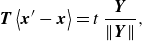
As an alternative formulation to the classical solid mechanics, the original PD employed the Lagrangian scheme, as illustrated in figure 1(b). In this scheme, neighbouring material points for a specific master point stay fixed, while the shape and size of the family evolve continually with deformation. The Lagrangian formulation is well-suited for solid mechanics applications where the small deformation assumption usually remains valid. However, it faces challenges when applied to fluid mechanics and problems involving significant deformation, as the shape of the family can become highly distorted. Under such circumstances, the derivatives in the governing equations are poorly evaluated by integration over material points within a distorted family. Semi-Lagrangian PD serves as a remedy to facilitate modelling of large deformation problems by PD. Also known as Eulerian PD (Silling et al. Reference Silling, Parks, Kamm, Weckner and Rassaian2017) or updated Lagrangian PD (Bergel & Li Reference Bergel and Li2016; Tu & Li Reference Tu and Li2017; Yan et al. Reference Yan, Li, Zhang, Kan and Sun2019, Reference Yan, Li, Kan, Zhang and Liu2021), it represents a relatively new variant of the traditional PD approach that combines both Lagrangian material points and Eulerian grids. In the semi-Lagrangian PD formulation, material points are still tracked using a Lagrangian approach, meaning that their positions, velocities and accelerations are explicitly updated at each time step. However, the interactions among the material points are computed using a Eulerian framework, where a fixed family shape is maintained, as illustrated in figure 1(c). This approach requires updating neighbouring material points in the presence of significant deformation, and derivatives are approximated using non-local integral operators. Two commonly used non-local operators are the non-local gradient operator $\mathbb{G}$
and the non-local divergence operator
$\mathbb{G}$
and the non-local divergence operator $\mathbb{D}$
, which uses integrations over neighbouring material points to approximate gradient and divergence at a specific material point. They are expressed as (Bergel & Li Reference Bergel and Li2016)
$\mathbb{D}$
, which uses integrations over neighbouring material points to approximate gradient and divergence at a specific material point. They are expressed as (Bergel & Li Reference Bergel and Li2016)
Schematics of (a) basic concepts and initial configuration of PD, (b) the total-Lagrangian scheme, and (c) the semi-Lagrangian scheme, taking a thermal expansion process as an example.
 \begin{align}& \mathbb{G}\left(\boldsymbol{A}\right)=\left[\int _{{B_{x}}}w\left\langle \left\| \boldsymbol{Y}\right\| \right\rangle \left({\unicode[Arial]{x0394}} \,{\boldsymbol{\cdot}}\, \boldsymbol{A}\right)\otimes \boldsymbol{Y}\,{\rm d}V_{x'}\right]\boldsymbol{M}_{x}^{-1}\cong {\boldsymbol{\nabla}} \boldsymbol{A}, \end{align}
 \begin{align}& \mathbb{D}\left(\boldsymbol{A}\right)=\int _{{B_{x}}}w\left\langle \left\| \boldsymbol{Y}\right\| \right\rangle \left({\unicode[Arial]{x0394}} \,{\boldsymbol{\cdot}}\, \boldsymbol{A}\right) {\boldsymbol{\cdot}} \left(\boldsymbol{M}_{x}^{-1}\boldsymbol{Y}\right)\,\mathrm{d}V_{x'}\cong {\boldsymbol{\nabla}} \,{\boldsymbol{\cdot}}\, \boldsymbol{A}, \end{align}
where $\boldsymbol{A}$
is a random vector. Here,
$\boldsymbol{A}$
is a random vector. Here, ${\unicode[Arial]{x0394}} \,{\boldsymbol{\cdot}}\,$
represents a difference operator, e.g.
${\unicode[Arial]{x0394}} \,{\boldsymbol{\cdot}}\,$
represents a difference operator, e.g. ${\unicode[Arial]{x0394}} \,{\boldsymbol{\cdot}}\, \boldsymbol{A}=\boldsymbol{A}_{x'}-\boldsymbol{A}_{x}$
;
${\unicode[Arial]{x0394}} \,{\boldsymbol{\cdot}}\, \boldsymbol{A}=\boldsymbol{A}_{x'}-\boldsymbol{A}_{x}$
; ${\boldsymbol{\nabla}} \boldsymbol{A}$
and
${\boldsymbol{\nabla}} \boldsymbol{A}$
and ${\boldsymbol{\nabla}} \,{\boldsymbol{\cdot}}\, \boldsymbol{A}$
represents the local gradient and local divergence of vector
${\boldsymbol{\nabla}} \,{\boldsymbol{\cdot}}\, \boldsymbol{A}$
represents the local gradient and local divergence of vector $\boldsymbol{A}$
, respectively;
$\boldsymbol{A}$
, respectively; $\otimes$
is the dyadic product; and
$\otimes$
is the dyadic product; and $\boldsymbol{M}_{x}$
is defined as the shape matrix, which is calculated as
$\boldsymbol{M}_{x}$
is defined as the shape matrix, which is calculated as
 \begin{equation}\boldsymbol{M}_{x}=\int _{{B_{x}}}w\left\langle \left\| \boldsymbol{Y}\right\| \right\rangle\, \boldsymbol{Y}\otimes \boldsymbol{Y}\, \mathrm{d}V_{x'},\end{equation}
in which $w\langle \| \boldsymbol{Y}\| \rangle$
is the weight function that determines the influence of neighbouring material points based on their distances to the master point. The weight function can be chosen in various forms, such as unity, B-spline or Gaussian functions. In this study,
$w\langle \| \boldsymbol{Y}\| \rangle$
is the weight function that determines the influence of neighbouring material points based on their distances to the master point. The weight function can be chosen in various forms, such as unity, B-spline or Gaussian functions. In this study, $w\langle \| \boldsymbol{Y}\| \rangle$
is specifically selected in the Gaussian form
$w\langle \| \boldsymbol{Y}\| \rangle$
is specifically selected in the Gaussian form
 \begin{equation}w\left\langle \left\| \boldsymbol{Y}\right\| \right\rangle =\exp\left({-{\left(\frac{\left\| \boldsymbol{Y}\right\| }{\alpha \delta }\right)^{2}}}\right),\end{equation}
where the parameter $\alpha$
is selected to be 0.5. Note that all the integrations in (2.3)–(2.5) are conducted over the updated family
$\alpha$
is selected to be 0.5. Note that all the integrations in (2.3)–(2.5) are conducted over the updated family $B_{x}$
.
$B_{x}$
.
3. Coupled thermo-hydrodynamic PD model
In this section, the governing equations for fluid flow coupled with heat transfer are reformulated into their non-local forms using the semi-Lagrangian PD method and non-local operators. The fluid flow is assumed to be weakly compressible, inviscid and heat conducting.
3.1. Continuity equation
The continuity equation required the conservation of mass within a fixed volume over time, which is given by
 \begin{equation}\frac{\partial \rho }{\partial t}+{\boldsymbol{\nabla}} \,{\boldsymbol{\cdot}}\, \left(\rho \boldsymbol{v}\right)=0,\end{equation}
where $\boldsymbol{v}$
is the velocity vector, and
$\boldsymbol{v}$
is the velocity vector, and $\partial /\partial t$
is the Eulerian derivative with respect to time. The term
$\partial /\partial t$
is the Eulerian derivative with respect to time. The term ${\boldsymbol{\nabla}} \,{\boldsymbol{\cdot}}\, (\rho \boldsymbol{v})$
can be further expanded to
${\boldsymbol{\nabla}} \,{\boldsymbol{\cdot}}\, (\rho \boldsymbol{v})$
can be further expanded to
 \begin{equation}\frac{\partial \rho }{\partial t}+\boldsymbol{v}\,{\boldsymbol{\cdot}}\, {\boldsymbol{\nabla}} \rho +\rho\, {\boldsymbol{\nabla}} \,{\boldsymbol{\cdot}}\, \boldsymbol{v}=0.\end{equation}
For isothermal flows, the density change, i.e. the second term on the left-hand side of (3.2), can be neglected. However, for thermal flows, where temperature variations occur, the density becomes a thermodynamic variable that is dependent on temperature. Therefore, all three terms in (3.2) should be considered explicitly for thermal flow.
To bridge the Eulerian and Lagrangian descriptions (note that semi-Lagrangian PD still adopts the Lagrangian description), the Lagrangian derivative (also known as the material derivative) is introduced as
 \begin{equation}\frac{\mathrm{D}}{\mathrm{D}t}=\frac{\partial }{\partial t}+\boldsymbol{v}\,{\boldsymbol{\cdot}}\, {\boldsymbol{\nabla}},\end{equation}
therefore the continuity equation given in (3.2) can be alternatively written in Lagrangian form as
 \begin{equation}\frac{\mathrm{D}\rho }{\mathrm{D}t}+\rho {\boldsymbol{\nabla}} \,{\boldsymbol{\cdot}}\, \boldsymbol{v}=0.\end{equation}
Note that (3.4) and (3.2) are fundamentally equivalent. The Lagrangian derivative (or material derivative) explicitly incorporates both the local change present in the Eulerian derivative and the convective change terms. This equivalence arises because the material derivative accounts for the temporal variation at a fixed point (local change) and the transport of the quantity due to fluid motion (convective change). Thus the two formulations describe the same physical process but from different perspectives.
In the case of incompressible flows, directly implementing (3.4) in an explicit scheme necessitates an extremely small time step, which is computationally prohibitive. To address this issue, a weakly compressible method proposed by Monaghan (Reference Monaghan1994) in SPH is utilized to model the incompressible fluid. In this approach, an equation of state is introduced to describe the relationship between the pressure $p$
and the density
$p$
and the density $\rho$
of the fluid:
$\rho$
of the fluid:
 \begin{equation}p=\frac{\rho c_{0}^{2}}{n}\left[\left(\frac{\rho }{\rho _{0}}\right)^{n}-1\right],\end{equation}
where $n$
is one fitting parameter, which can be interpreted from experiments,
$n$
is one fitting parameter, which can be interpreted from experiments, $\rho _{0}$
is the initial density, and
$\rho _{0}$
is the initial density, and $c_{0}$
is the artificial sound speed. By using the weakly compressible method, the density is updated according to (3.4), and the pressure is calculated explicitly from (3.5). Substituting the non-local divergence operator given in (2.4) into (3.4) gives the non-local continuity equation as
$c_{0}$
is the artificial sound speed. By using the weakly compressible method, the density is updated according to (3.4), and the pressure is calculated explicitly from (3.5). Substituting the non-local divergence operator given in (2.4) into (3.4) gives the non-local continuity equation as
 \begin{equation}\frac{\mathrm{D}\rho }{\mathrm{D}t}=-\rho \int _{{B_{x}}}\omega \left\langle \left\| \boldsymbol{Y}\right\| \right\rangle\, \boldsymbol{v} \left\langle \boldsymbol{Y}\right\rangle \,{\boldsymbol{\cdot}}\, \left(\boldsymbol{M}_{x}^{-1}\boldsymbol{Y}\right)\mathrm{d}V_{x'}.\end{equation}
3.2. Momentum equation
The classical local equation of motion is expressed mathematically as
 \begin{equation}\frac{\partial \rho \boldsymbol{v}}{\partial t}+{\boldsymbol{\nabla}} \,{\boldsymbol{\cdot}}\, \left(\rho \boldsymbol{v}\otimes \boldsymbol{v}\right)={\boldsymbol{\nabla}} \,{\boldsymbol{\cdot}}\, \boldsymbol{\sigma }+\boldsymbol{b},\end{equation}
where $\boldsymbol{\sigma }$
is the Cauchy stress tensor, and
$\boldsymbol{\sigma }$
is the Cauchy stress tensor, and $\boldsymbol{b}$
denotes the body force density. Equation (3.7) governs the motion of a continuous medium and is more commonly known as the Navier equation in fluid mechanics. For incompressible fluid, (3.7) can be further simplified by expanding the two derivatives on the left-hand side,
$\boldsymbol{b}$
denotes the body force density. Equation (3.7) governs the motion of a continuous medium and is more commonly known as the Navier equation in fluid mechanics. For incompressible fluid, (3.7) can be further simplified by expanding the two derivatives on the left-hand side,
 \begin{equation}\rho \left(\frac{\partial \boldsymbol{v}}{\partial t}+\boldsymbol{v}\,{\boldsymbol{\nabla}} \,{\boldsymbol{\cdot}}\, \boldsymbol{v}\right)={\boldsymbol{\nabla}} \,{\boldsymbol{\cdot}}\, \boldsymbol{\sigma }+\rho \boldsymbol{g},\end{equation}
or expressed in the Lagrangian description with the material derivative,
 \begin{equation}\rho\, \frac{\mathrm{D}\boldsymbol{v}}{\mathrm{D}t}={\boldsymbol{\nabla}} \,{\boldsymbol{\cdot}}\, \boldsymbol{\sigma }+\rho \boldsymbol{g}.\end{equation}
In the case of thermal flow, temperature variations can lead to changes in fluid properties such as density and viscosity. The Boussinesq approximation is a commonly adopted approach in which the variations of all fluid properties, except for density differences multiplied by the acceleration due to gravity, i.e. $\rho \boldsymbol{g}$
in (3.8)–(3.9), are neglected. This approximation allows for a computationally efficient simulation while effectively capturing the buoyancy force resulting from temperature changes. However, it is important to note that the Boussinesq approximation requires small variations in both temperature and density to be valid. In this study, instead of using the Boussinesq approximation, we update the density in each step according to (3.4), then consider the thermal effect by incorporating the expression
$\rho \boldsymbol{g}$
in (3.8)–(3.9), are neglected. This approximation allows for a computationally efficient simulation while effectively capturing the buoyancy force resulting from temperature changes. However, it is important to note that the Boussinesq approximation requires small variations in both temperature and density to be valid. In this study, instead of using the Boussinesq approximation, we update the density in each step according to (3.4), then consider the thermal effect by incorporating the expression
 \begin{equation}\rho =\rho '+{\unicode[Arial]{x0394}} \rho,\end{equation}
where $\rho '$
denotes the initial density obtained directly from (3.4) at each step, and
$\rho '$
denotes the initial density obtained directly from (3.4) at each step, and ${\unicode[Arial]{x0394}} \rho$
is the variation of density induced by variation in temperature. Provided that the variation in density is linearly related to the variation in temperature,
${\unicode[Arial]{x0394}} \rho$
is the variation of density induced by variation in temperature. Provided that the variation in density is linearly related to the variation in temperature, ${\unicode[Arial]{x0394}} \rho$
can be expressed as a function of thermal expansion coefficient
${\unicode[Arial]{x0394}} \rho$
can be expressed as a function of thermal expansion coefficient $\beta$
as
$\beta$
as
 \begin{equation}{\unicode[Arial]{x0394}}\rho =-\beta\,{\unicode[Arial]{x0394}}\Theta\,\rho ',\end{equation}
in which ${\unicode[Arial]{x0394}} \Theta$
is the variation in temperature. Note that the density is assumed to decrease monotonically as temperature increases. If the density–temperature relationship is nonlinear and requires a more complex expression, then it is possible to introduce more intricate equations to capture the behaviour accurately (Szewc et al. Reference Szewc, Pozorski and Tanière2011).
${\unicode[Arial]{x0394}} \Theta$
is the variation in temperature. Note that the density is assumed to decrease monotonically as temperature increases. If the density–temperature relationship is nonlinear and requires a more complex expression, then it is possible to introduce more intricate equations to capture the behaviour accurately (Szewc et al. Reference Szewc, Pozorski and Tanière2011).
The momentum equation can also be expressed in non-local form by substituting (2.4) into (3.9):
 \begin{equation}\rho\, \frac{\mathrm{D}\boldsymbol{v}}{\mathrm{D}t}=\int _{{B_{x}}}\omega \left\langle \left\| \boldsymbol{Y}\right\| \right\rangle \left(\boldsymbol{\sigma }_{x}\boldsymbol{M}_{x}^{-1}+\boldsymbol{\sigma }_{x'}\boldsymbol{M}_{x'}^{-1}\right)\boldsymbol{Y}\, \mathrm{d}V_{x'}+\boldsymbol{b}.\end{equation}
3.3. Constitutive equation of fluid
For the Newtonian fluid considered in this paper, the stress tensor $\boldsymbol{\sigma }$
in (3.9) can be decomposed into two parts:
$\boldsymbol{\sigma }$
in (3.9) can be decomposed into two parts:
 \begin{equation}\boldsymbol{\sigma }=-p\boldsymbol{I}+2\mu \dot{\boldsymbol{\varepsilon }},\end{equation}
where the pressure $p$
represents the hydrostatic part and can be calculated by the equation of state defined in (3.5),
$p$
represents the hydrostatic part and can be calculated by the equation of state defined in (3.5), $\mu$
is the dynamic viscosity, and
$\mu$
is the dynamic viscosity, and $\dot{\boldsymbol{\varepsilon }}$
is the rate of deformation, the product of these latter two denoting the viscous part. Here,
$\dot{\boldsymbol{\varepsilon }}$
is the rate of deformation, the product of these latter two denoting the viscous part. Here, $\dot{\boldsymbol{\varepsilon }}$
can be related to the gradient of velocity as
$\dot{\boldsymbol{\varepsilon }}$
can be related to the gradient of velocity as
 \begin{equation}\dot{\boldsymbol{\varepsilon }}=\tfrac{1}{2}\left[{\boldsymbol{\nabla}} \boldsymbol{v}+\left({\boldsymbol{\nabla}} \boldsymbol{v}\right)^{\mathrm{T}}\right].\end{equation}
3.4. Energy equation
When considering heat transfer, the fluid flow system is extended by incorporating the energy equation, which states that the time rate of change of the total energy is
 \begin{equation}\rho \left(\frac{\partial e}{\partial t}+\boldsymbol{v}\,{\boldsymbol{\nabla}} \,{\boldsymbol{\cdot}}\, e\right)=-{\boldsymbol{\nabla}} \,{\boldsymbol{\cdot}}\, \boldsymbol{q}+\varphi +\rho \Theta _{{b}},\end{equation}
where $\Theta _{{b}}$
is the internal volumetric heat generation per unit mass, the dissipation function
$\Theta _{{b}}$
is the internal volumetric heat generation per unit mass, the dissipation function $\varphi =2\mu \dot{\boldsymbol{\varepsilon }}\colon \dot{\boldsymbol{\varepsilon }}$
is adopted according to Reddy & Gartling (Reference Reddy and Gartling2010), and the heat flux
$\varphi =2\mu \dot{\boldsymbol{\varepsilon }}\colon \dot{\boldsymbol{\varepsilon }}$
is adopted according to Reddy & Gartling (Reference Reddy and Gartling2010), and the heat flux $\boldsymbol{q}$
is defined as
$\boldsymbol{q}$
is defined as
 \begin{equation}\boldsymbol{q}=-k_{{h}}\,{\boldsymbol{\nabla}} \Theta,\end{equation}
in which $k_{{h}}$
is the thermal conductivity. For the internal energy function
$k_{{h}}$
is the thermal conductivity. For the internal energy function $e$
, one of the most common expressions is as a function of temperature and density, i.e.
$e$
, one of the most common expressions is as a function of temperature and density, i.e. $e=e(\Theta, \rho )$
. The derivative of
$e=e(\Theta, \rho )$
. The derivative of $e$
with respect to time can be expanded according to the chain rule as
$e$
with respect to time can be expanded according to the chain rule as
 \begin{equation}\frac{\partial e}{\partial t}=\frac{\partial e}{\partial \Theta }\frac{\mathrm{D}\Theta }{\mathrm{D}t}+\frac{\partial e}{\partial \rho }\frac{\mathrm{D}\rho }{\mathrm{D}t},\end{equation}
where $\partial e/\partial \Theta$
is defined as the specific heat capacity
$\partial e/\partial \Theta$
is defined as the specific heat capacity $c$
, and
$c$
, and $\mathrm{D}\rho$
can be regarded as zero for incompressible fluid considered in this paper. Therefore, substituting (3.17) into (3.15)–(3.16) yields the non-local energy equation and non-local Fourier law:
$\mathrm{D}\rho$
can be regarded as zero for incompressible fluid considered in this paper. Therefore, substituting (3.17) into (3.15)–(3.16) yields the non-local energy equation and non-local Fourier law:
 \begin{align}& \rho c\frac{\mathrm{D}\Theta }{\mathrm{D}t}=\int _{{B_{x}}}\omega \left\langle \left\| \boldsymbol{Y}\right\| \right\rangle \left(\boldsymbol{q}_{x}\boldsymbol{M}_{x}^{-1}+\boldsymbol{q}_{x\boldsymbol{'}}\boldsymbol{M}_{x'}^{-1}\right)\boldsymbol{Y}\,{\rm d}V_{x'}+\varphi +\rho \Theta _{{b}}, \end{align}
 \begin{align}&\qquad\qquad \boldsymbol{q}_{\boldsymbol{x}}=-k_{{h}}\left[\int _{{B_{x}}}\omega \left\langle \left\| \boldsymbol{Y}\right\| \right\rangle \left({\unicode[Arial]{x0394}} \,{\boldsymbol{\cdot}}\, \Theta \right) \boldsymbol{Y}\,\mathrm{d}V_{x'}\right]\boldsymbol{M}_{x}^{-1}. \end{align}
4. Multi-horizon scheme and numerical implementation
Section 3 provides a detailed formulation of the coupled thermo-hydrodynamic PD model, which can be readily used to model convection problems. However, our previous research on the dispersion relation and error analysis of the PD heat equation (Yang et al. Reference Yang, Zhu and Zhao2024a ) has highlighted the significant impact of non-locality on the accuracy of thermal field modelling. Specifically, as the horizon size increases, the ratio of heat conduction slows down, and there is a potential for oscillations in the temperature field. This phenomenon occurs because the non-local PD formulation allows particles to bypass heat flux, which is inconsistent with the fundamental nature of heat conduction, a process that is inherently local and relies on direct contact. It is worth noting that the previous investigation was based on a total-Lagrangian scheme, and the situation may be even more challenging with a semi-Lagrangian scheme due to the additional errors arising from irregularly distributed material points. With these considerations, it is favourable to use a small horizon for the thermal field, since a small horizon helps to mitigate the potential issues associated with non-local effects as mentioned above.
On the other hand, the convection process in thermal flow can exhibit highly non-local behaviour. In fluid flow systems, convection can induce changes in density and velocity profiles throughout the fluid domain. While these changes originate from local heat conduction, they can occur over a larger spatial extent, especially in extreme cases such as Earth’s atmosphere and mantle, spanning hundreds of kilometres (Huang Reference Huang2024). Since density and velocity are crucial factors in determining flow behaviours of fluids, it is essential to select a horizon size for fluid flow modelling that is large enough to capture the convective characteristics. According to the numerical experiments conducted by Reece et al. (Reference Reece, Rogers, Fourtakas and Lind2024), a kernel smoothing length of four times the particle size is required to accurately capture the steady-state thermal flow in SPH. Similarly, based on our experience, it is recommended that the horizon for fluid flow modelling in PD should be at least three times the material point size, with four or five times acceptable, to effectively capture the complex convective pattern. However, this poses a dilemma when it comes to modelling thermal flow, as a smaller horizon is preferable to the heat conduction process.
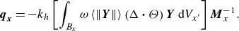
To address the challenge of maintaining accuracy and stability for both fluid and thermal field modelling, a multi-horizon scheme has been employed in this study. This approach, first proposed by Yang et al. (Reference Yang, Zhu and Zhao2024a ) in coupled thermo-mechanical problems, involves using a larger horizon for solid fracturing modelling, and a smaller horizon for heat transfer modelling. In the context of coupled flow and heat transfer processes, a larger horizon is adopted for modelling fluid motion, while a smaller one, termed the thermal horizon, is used for heat conduction. The larger fluid horizon captures convective behaviour and changes in density and velocity profiles over a larger spatial extent, while the smaller thermal horizon focuses on localized heat conduction and mitigates dispersive issues in thermal modelling. This approach allows us to achieve optimized accuracy in both fluid and thermal aspects by considering their distinct characteristics. The multi-horizon scheme also serves as a way to save computational cost as fewer neighbouring material points are involved in the thermal field model. A schematic diagram illustrating the methodology is presented in figure 2.
Schematics of the semi-Lagrangian multi-horizon thermo-hydrodynamic PD model: family of material point (MP) i (initial ${\Omega} _{i}$
and updated
${\Omega} _{i}$
and updated ${B}_{i}$
), and thermal horizon of material point j (initial
${B}_{i}$
), and thermal horizon of material point j (initial ${\Omega} _{j}^{\prime}$
and updated
${\Omega} _{j}^{\prime}$
and updated ${B}_{j}'$
).
${B}_{j}'$
).
4.1. Spatial discretization
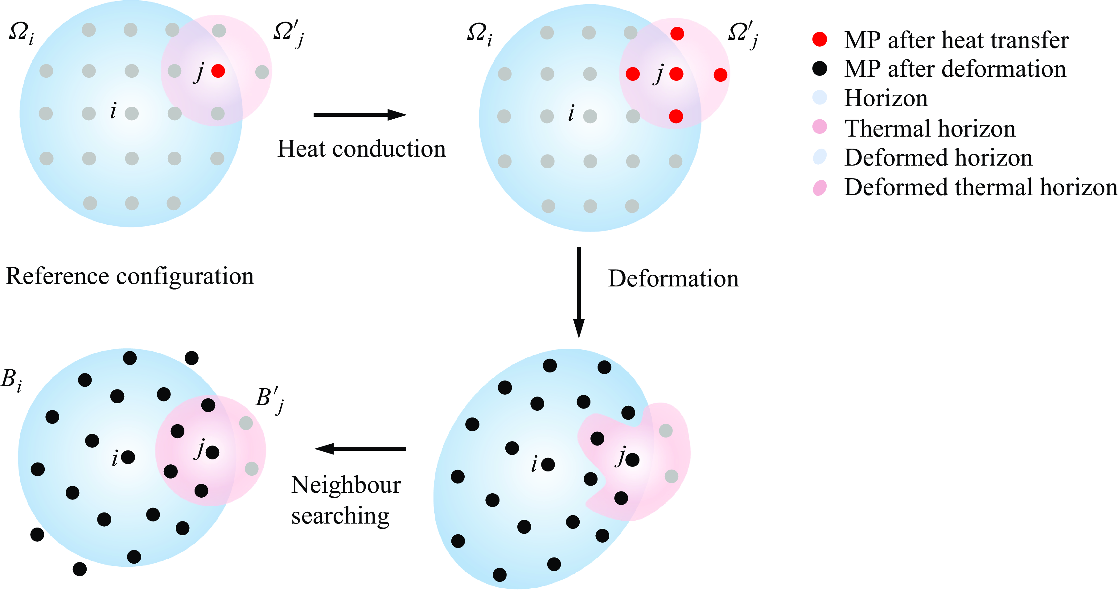
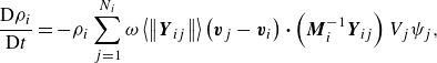
To solve the integral governing equations, the entire simulation domain must be discretized into subdomains. Typically, line segments, squares and cubes are used as subdomains for one-dimensional (1-D), 2-D and 3-D problems, respectively. After discretization, material points are placed at the centroids of these subdomains. All calculations are performed at these material points, which are analogous to Gaussian points in the FEM. However, these material points carry all material properties as well as the volume (or area/length for 2-D/1-D problems) of their respective subdomains. For clarity, figure 3 illustrates the discretization of a 2-D problem with uniform spacing ${\unicode[Arial]{x0394}} x$
between material points. Using this meshless discretization scheme, (3.6), (3.12), (3.18) and (3.19) can be expressed in the discretized form as
${\unicode[Arial]{x0394}} x$
between material points. Using this meshless discretization scheme, (3.6), (3.12), (3.18) and (3.19) can be expressed in the discretized form as
Discretization, material points and volume correction in a 2-D problem.
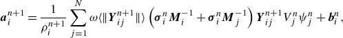
 \begin{align}&\quad \frac{\mathrm{D}\rho _{i}}{\mathrm{D}t}=-\rho _{i}\sum _{j=1}^{N_{i}}\omega \left\langle \left\| \boldsymbol{Y}_{ij}\right\| \right\rangle \left(\boldsymbol{v}_{j}-\boldsymbol{v}_{i}\right) {\boldsymbol{\cdot}} \left(\boldsymbol{M}_{i}^{-1}\boldsymbol{Y}_{ij}\right)V_{j}\psi _{j},\end{align}
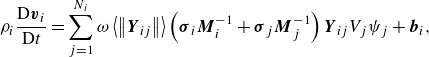 \begin{align}&\rho _{i}\frac{\mathrm{D}\boldsymbol{v}_{i}}{\mathrm{D}t}=\sum _{j=1}^{N_{i}}\omega \left\langle \left\| \boldsymbol{Y}_{ij}\right\| \right\rangle \left(\boldsymbol{\sigma }_{i}\boldsymbol{M}_{i}^{-1}+\boldsymbol{\sigma }_{j}\boldsymbol{M}_{j}^{-1}\right)\boldsymbol{Y}_{ij}V_{j}\psi _{j}+\boldsymbol{b}_{i}, \end{align}
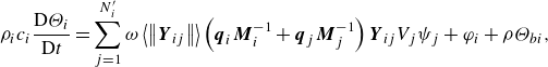 \begin{align}&\rho _{i}c_{i}\frac{\mathrm{D}\Theta _{i}}{\mathrm{D}t}=\sum _{j=1}^{N_{i}'}\omega \left\langle \left\| \boldsymbol{Y}_{ij}\right\| \right\rangle \left(\boldsymbol{q}_{i}\boldsymbol{M}_{i}^{-1}+\boldsymbol{q}_{j}\boldsymbol{M}_{j}^{-1}\right)\boldsymbol{Y}_{ij}V_{j}\psi _{j}+\varphi _{i}+\rho \Theta _{{b}i}, \end{align}
 \begin{align}&\qquad\qquad \boldsymbol{q}_{i}=-k_{{h}}\left[\sum _{j=1}^{N_{i}'}\omega \left\langle \left\| \boldsymbol{Y}_{ij}\right\| \right\rangle \left(\Theta _{j}-\Theta _{i}\right)\boldsymbol{Y}_{ij}V_{j}\psi _{j}\right]\boldsymbol{M}_{i}^{-1}, \end{align}
where the subscripts $i$
and
$i$
and $j$
are associated with master material point
$j$
are associated with master material point $i$
and neighbouring material point
$i$
and neighbouring material point $j,$
respectively. Here,
$j,$
respectively. Here, $N$
represents family number within the fluid horizon, while
$N$
represents family number within the fluid horizon, while $N'$
represents family number within the thermal horizon. The deformed bond vector between
$N'$
represents family number within the thermal horizon. The deformed bond vector between $i$
and
$i$
and $j$
,
$j$
, $\boldsymbol{Y}_{ij}$
, is calculated by
$\boldsymbol{Y}_{ij}$
, is calculated by $\boldsymbol{x}_{j}-\boldsymbol{x}_{i}$
. Also,
$\boldsymbol{x}_{j}-\boldsymbol{x}_{i}$
. Also, $\psi _{j}$
is a volume correction coefficient since the outer neighbouring material points within the range
$\psi _{j}$
is a volume correction coefficient since the outer neighbouring material points within the range $\delta -{\unicode[Arial]{x0394}} x/2\lt \| \boldsymbol{Y}_{ij}\| \lt \delta$
are only partially enclosed within the horizon, as illustrated in figure 3. The correction coefficient
$\delta -{\unicode[Arial]{x0394}} x/2\lt \| \boldsymbol{Y}_{ij}\| \lt \delta$
are only partially enclosed within the horizon, as illustrated in figure 3. The correction coefficient $\psi _{j}$
is defined according to the distance between two material points as (Silling & Askari Reference Silling and Askari2005)
$\psi _{j}$
is defined according to the distance between two material points as (Silling & Askari Reference Silling and Askari2005)
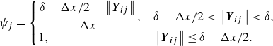 \begin{equation}\psi _{j}=\begin{cases} \dfrac{\delta -{\unicode[Arial]{x0394}} x/2-\left\| \boldsymbol{Y}_{ij}\right\| }{{\unicode[Arial]{x0394}} x}, & \delta -{\unicode[Arial]{x0394}} x/2\lt \left\| \boldsymbol{Y}_{ij}\right\| \lt \delta, \\ 1, & \left\| \boldsymbol{Y}_{ij}\right\| \leq \delta -{\unicode[Arial]{x0394}} x/2. \end{cases}\end{equation}
4.2. Time integration
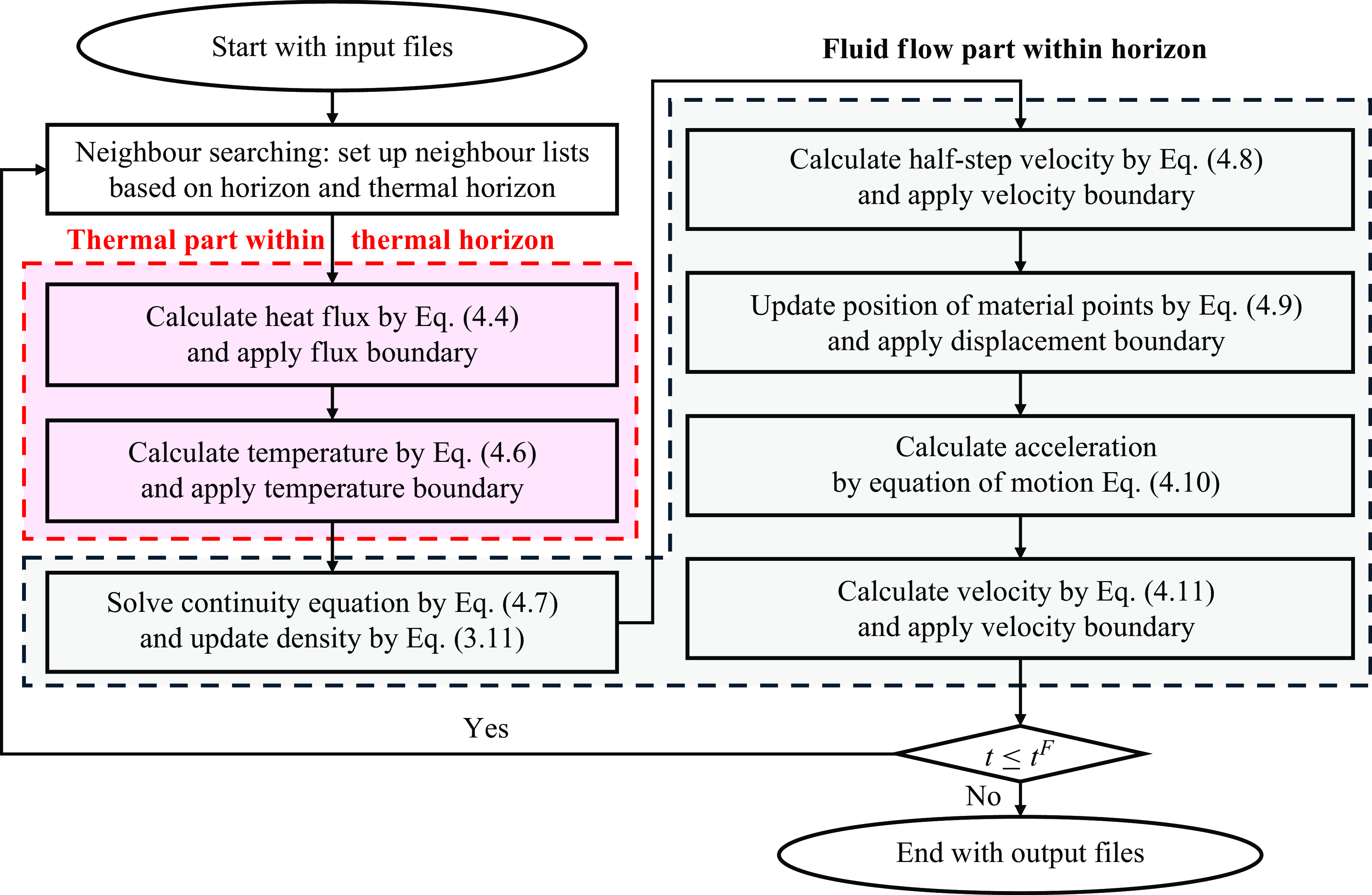
To numerically obtain the solution to the coupled thermo-hydrodynamic system, the coupled PD equations are partitioned naturally according to fluid flow field and thermal field, and each field is solved sequentially by a forward difference scheme. The procedure involves a series of steps as illustrated in the flow chart in figure 4. In each time step, the heat equation is initially solved within the thermal horizon using a forward difference scheme:
Flow chart of the time integration of the multi-horizon scheme.
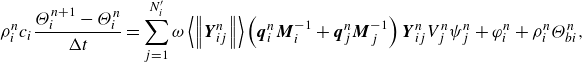 \begin{equation}\rho _{i}^{n}c_{i}\frac{\Theta _{i}^{n+1}-\Theta _{i}^{n}}{{\unicode[Arial]{x0394}} t}=\sum _{j=1}^{N_{i}'}\omega \left\langle \left\| \boldsymbol{Y}_{ij}^{n}\right\| \right\rangle \left(\boldsymbol{q}_{i}^{n}\boldsymbol{M}_{i}^{-1}+\boldsymbol{q}_{j}^{n}\boldsymbol{M}_{j}^{-1}\right)\boldsymbol{Y}_{ij}^{n}V_{j}^{n}\psi _{j}^{n}+\varphi _{i}^{n}+\rho _{i}^{n}\Theta _{{b}i}^{n},\end{equation}
where the superscript $n$
denotes the values at the
$n$
denotes the values at the $n$
th step, and
$n$
th step, and ${\unicode[Arial]{x0394}} t$
is the time step. This computation enables the update of temperatures for material points within the thermal horizon while keeping the positions of all material points unchanged.
${\unicode[Arial]{x0394}} t$
is the time step. This computation enables the update of temperatures for material points within the thermal horizon while keeping the positions of all material points unchanged.
Subsequently, the continuity and momentum equations are solved within the fluid horizon also by a forward difference scheme:
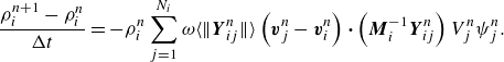 \begin{equation}\frac{\rho _{i}^{n+1}-\rho _{i}^{n}}{{\unicode[Arial]{x0394}} t}=-\rho _{i}^{n}\sum _{j=1}^{N_{i}}\omega \Big\langle \Big\| \boldsymbol{Y}_{ij}^{n}\Big\| \Big\rangle \left(\boldsymbol{v}_{j}^{n}-\boldsymbol{v}_{i}^{n}\right) {\boldsymbol{\cdot}} \left(\boldsymbol{M}_{i}^{-1}\boldsymbol{Y}_{ij}^{n}\right)V_{j}^{n}\psi _{j}^{n}.\end{equation}
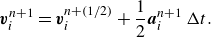
In this step, the new temperatures obtained from the heat equation solution are used. The position, velocity and acceleration of the material points are then updated accordingly by the velocity Verlet scheme:
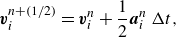 \begin{align}&\qquad\qquad\qquad\qquad\qquad\quad \boldsymbol{v}_{i}^{n+({1}/{2})}=\boldsymbol{v}_{i}^{n}+\frac{1}{2}\boldsymbol{a}_{i}^{n}\,{\unicode[Arial]{x0394}} t, \end{align}
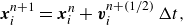 \begin{align}&\qquad\qquad\qquad\qquad\qquad\quad \boldsymbol{x}_{i}^{n+1}=\boldsymbol{x}_{i}^{n}+\boldsymbol{v}_{i}^{n+({1}/{2})}\,{\unicode[Arial]{x0394}} t, \end{align}
 \begin{align}& \boldsymbol{a}_{i}^{n+1}=\frac{1}{\rho _{i}^{n+1}}\sum _{j=1}^{N}\omega \Big\langle \Big\| \boldsymbol{Y}_{ij}^{n+1}\Big\| \Big\rangle \left(\boldsymbol{\sigma }_{i}^{n}\boldsymbol{M}_{i}^{-1}+\boldsymbol{\sigma }_{i}^{n}\boldsymbol{M}_{j}^{-1}\right)\boldsymbol{Y}_{ij}^{n+1}V_{j}^{n}\psi _{j}^{n}+\boldsymbol{b}_{i}^{n}, \end{align}
 \begin{align}&\qquad\qquad\qquad\qquad\qquad \boldsymbol{v}_{i}^{n+1}=\boldsymbol{v}_{i}^{n+({1}/{2})}+\frac{1}{2}\boldsymbol{a}_{i}^{n+1}\,{\unicode[Arial]{x0394}} t. \end{align}
In scenarios involving large deformation problems, such as fluid flow, it is important to note that both the fluid horizon and thermal horizon can become significantly distorted after updating the positions of the material points. As a result, an additional neighbour searching process is necessary in the semi-Lagrangian scheme. During this process, the neighbouring material points of a given master point are updated while preserving the circular shape of both the fluid horizon and the thermal horizon. For a visual representation of the described methodology, see figure 2. Since neighbour searching must be performed at each time step due to the continuous motion of material points, selecting an efficient neighbour-searching algorithm is critical for minimizing computational costs. In this study, we adopt the region partition search algorithm, as elaborated in Madenci & Oterkus (Reference Madenci and Oterkus2014) and Diyaroglu (Reference Diyaroglu2016). The primary concept of the region partition search algorithm is to divide the entire domain into equally sized cells that are larger than the horizon. When searching for neighbouring material points, it is only necessary to examine the neighbouring cells, while deactivating all the material points in non-neighbouring cells. The region partition search algorithm has been proven to outperform several other searching algorithms with different tree structures (Vazic et al. Reference Vazic, Diyaroglu, Oterkus and Oterkus2020). While there may be more advanced searching algorithms that offer superior computational efficiency, optimizing the searching algorithm is beyond the scope of this paper.
4.3. Implementation of boundary conditions
In numerical simulations, displacement, velocity and temperature boundary conditions can be implemented directly by introducing additional material points as non-local Dirichlet boundary conditions. For non-isothermal problems, adiabatic or flux boundary conditions are also commonly required. Flux boundary conditions are typically treated as Neumann boundary conditions. Madenci & Oterkus (Reference Madenci and Oterkus2014) proposed a method for implementing non-local flux boundary conditions by adding extra material points and prescribing their temperatures at each time step; however, this approach significantly increases computational costs.
In this study, we adopt a two-field formulation of the energy equation, as shown in (3.18) and (3.19), which explicitly expresses the governing equation for flux. This formulation allows flux boundary conditions to be imposed directly by prescribing the flux (Dirichlet boundary) rather than indirectly through temperature (Neumann boundary). Macek & Silling (Reference Macek and Silling2007) recommended that the extent of additional material points should match the horizon size $\delta$
to ensure that boundary conditions are adequately reflected within the simulation domain. In the multi-horizon scheme used in this work, displacement and velocity boundaries are applied using three layers of material points, while only one layer of material points is sufficient for thermal boundaries.
$\delta$
to ensure that boundary conditions are adequately reflected within the simulation domain. In the multi-horizon scheme used in this work, displacement and velocity boundaries are applied using three layers of material points, while only one layer of material points is sufficient for thermal boundaries.
4.4. Numerical stabilization
Due to the discretized nature of material points in semi-Lagrangian PD, they can sometimes become unevenly distributed or cluster together, leading to inaccurate results or program errors. To mitigate this issue, the particle shifting technique is employed. It involves adjusting the positions of material points during the simulation to alleviate clustering and improve the overall distribution. The shifting process typically includes two main steps. First, the density of each particle is estimated based on its neighbouring material points as
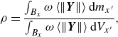 \begin{equation}\rho =\frac{\int _{{B_{x}}}\omega \left\langle \left\| \boldsymbol{Y}\right\| \right\rangle \mathrm{d}m_{x'}}{\int _{{B_{x}}}\omega \left\langle \left\| \boldsymbol{Y}\right\| \right\rangle \mathrm{d}V_{x'}},\end{equation}
where $m_{x'}$
and
$m_{x'}$
and $V_{x'}$
represent the mass and volume of a neighbouring material point, respectively. Particles that are too close to each other or have higher densities are shifted or moved slightly to achieve a more uniform distribution. The shifting is performed by applying corrective displacements to each material points as (Yang et al. Reference Yang, Zhu and Zhao2024a
)
$V_{x'}$
represent the mass and volume of a neighbouring material point, respectively. Particles that are too close to each other or have higher densities are shifted or moved slightly to achieve a more uniform distribution. The shifting is performed by applying corrective displacements to each material points as (Yang et al. Reference Yang, Zhu and Zhao2024a
)
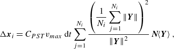 \begin{equation}{\unicode[Arial]{x0394}} \boldsymbol{x}_{i}=C_{{PST}}v_{max }\,\mathrm{d}t\sum _{j=1}^{N_{i}}\frac{\left(\dfrac{1}{N_{i}}\displaystyle\sum _{j=1}^{N_{i}}\left\| \boldsymbol{Y}\right\| \right)^{2}}{\left\| \boldsymbol{Y}\right\| ^{2}}\,\boldsymbol{N}\!\!\left\langle \boldsymbol{Y}\right\rangle,\end{equation}
where $C_{{PST}}$
is a shifting coefficient,
$C_{{PST}}$
is a shifting coefficient, $v_{max }$
represents the maximum expected velocity of fluid material points throughout the computational domain, and
$v_{max }$
represents the maximum expected velocity of fluid material points throughout the computational domain, and $\boldsymbol{N}\langle \boldsymbol{Y}\rangle$
denotes the unit vector of the deformed bond.
$\boldsymbol{N}\langle \boldsymbol{Y}\rangle$
denotes the unit vector of the deformed bond.
5. Benchmarks
5.1. Pure heat conduction of fluid in a square cavity
The natural convection within a closed square cavity serves as a typical case for modelling convective processes. To validate the proposed multi-horizon thermo-hydrodynamic PD model and semi-Lagrangian scheme for heat transfer, we first simulate pure heat conduction in the same square cavity before attempting to capture convective characteristics.
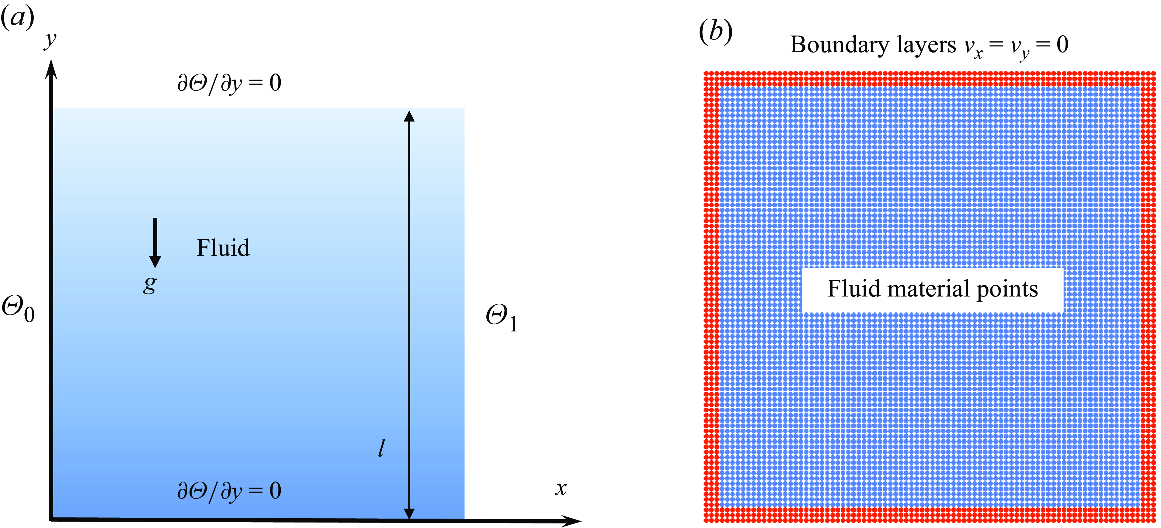
The schematic illustration of the square cavity is shown in figure 5 with both the width and length $l$
equal to 1 m. The initial temperature of the whole cavity is set as 0 °C. The temperatures of the left and right boundaries are fixed at 1 °C and 0 °C, respectively. The upper and lower boundaries are assumed to be adiabatic. All four surfaces are fixed by setting the velocity in both
$l$
equal to 1 m. The initial temperature of the whole cavity is set as 0 °C. The temperatures of the left and right boundaries are fixed at 1 °C and 0 °C, respectively. The upper and lower boundaries are assumed to be adiabatic. All four surfaces are fixed by setting the velocity in both $x$
and
$x$
and $y$
directions to zero. These non-local boundary conditions are applied by adding additional material points outside the modelling domain as shown in figure 5(b). Following the multi-horizon scheme, the horizon for fluid flow is adopted to be three times the material point size, while the thermal horizon for heat transfer is chosen as 1.5 times the material point size. Note that for thermal flow modelling, the thermal horizon cannot be adopted as only one time material point size as used in thermo-mechanical problems of solids by Yang et al. (Reference Yang, Zhu and Zhao2024a
). Owing to the large deformation nature of fluid flow, the material points can be randomly distributed within the domain. If the thermal horizon is set as only one time point size, then there might be no neighbouring material points in a certain direction, and an instability problem may be induced. The whole model is consequently discretized into
$y$
directions to zero. These non-local boundary conditions are applied by adding additional material points outside the modelling domain as shown in figure 5(b). Following the multi-horizon scheme, the horizon for fluid flow is adopted to be three times the material point size, while the thermal horizon for heat transfer is chosen as 1.5 times the material point size. Note that for thermal flow modelling, the thermal horizon cannot be adopted as only one time material point size as used in thermo-mechanical problems of solids by Yang et al. (Reference Yang, Zhu and Zhao2024a
). Owing to the large deformation nature of fluid flow, the material points can be randomly distributed within the domain. If the thermal horizon is set as only one time point size, then there might be no neighbouring material points in a certain direction, and an instability problem may be induced. The whole model is consequently discretized into $86 \times 86$
Lagrangian material points, each of size 0.0125 m.
$86 \times 86$
Lagrangian material points, each of size 0.0125 m.
Natural convection in a closed square cavity: (a) thermal boundary conditions and body force; (b) discretized PD model and velocity boundary conditions.
The fluid is assumed to be dry air, which has the following properties: density $\rho =1.3082$
kg m−3, viscosity
$\rho =1.3082$
kg m−3, viscosity $\mu =1.7\times 10^{-5}$
Pa s, thermal conductivity
$\mu =1.7\times 10^{-5}$
Pa s, thermal conductivity $k_{{h}}=0.024$
W m
$k_{{h}}=0.024$
W m $^{-1}$
°C
$^{-1}$
°C $^{-1}$
, specific heat
$^{-1}$
, specific heat $c_{{v}}=1005$
J kg
$c_{{v}}=1005$
J kg $^{-1}$
°C
$^{-1}$
°C $^{-1}$
, and thermal expansion coefficient
$^{-1}$
, and thermal expansion coefficient $\beta =0.00343$
°C−1 (McQuillan, Culham & Yovanovich Reference McQuillan, Culham and Yovanovich1984). For thermal flow, there are two relevant dimensionless quantities. One is the Prandtl number, defined as
$\beta =0.00343$
°C−1 (McQuillan, Culham & Yovanovich Reference McQuillan, Culham and Yovanovich1984). For thermal flow, there are two relevant dimensionless quantities. One is the Prandtl number, defined as
 \begin{equation}\Pr =\frac{\nu }{\alpha },\end{equation}
which describes the ratio of momentum diffusivity $\nu =\mu /\rho$
to thermal diffusivity
$\nu =\mu /\rho$
to thermal diffusivity $\alpha =k_{{h}}/\rho c$
. The properties of dry air adopted here give Prandtl number 0.71, which implies that the heat diffuses faster than momentum, leading to a more rapid temperature variation within fluid flow. Another important dimensionless quantity is the Rayleigh number, given by
$\alpha =k_{{h}}/\rho c$
. The properties of dry air adopted here give Prandtl number 0.71, which implies that the heat diffuses faster than momentum, leading to a more rapid temperature variation within fluid flow. Another important dimensionless quantity is the Rayleigh number, given by
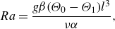 \begin{equation}{Ra}=\frac{g\beta\!\left(\Theta _{0}-\Theta _{1}\right)\!l^{3}}{\nu \alpha },\end{equation}
where $g$
is gravity,
$g$
is gravity, $\Theta _{0}-\Theta _{1}$
represents the temperature difference across the cavity, and
$\Theta _{0}-\Theta _{1}$
represents the temperature difference across the cavity, and $l$
is a characteristic length of the fluid domain. The Rayleigh number quantifies the tendency of a fluid to undergo convective motion due to thermal gradients. A larger Rayleigh number indicates more significant convection driven by buoyancy forces. In a zero-gravity environment, the fluid is free from external forces, resulting in Rayleigh number zero. Consequently, the combined conduction–convection process simplifies to pure conduction under this circumstance. In this subsection,
$l$
is a characteristic length of the fluid domain. The Rayleigh number quantifies the tendency of a fluid to undergo convective motion due to thermal gradients. A larger Rayleigh number indicates more significant convection driven by buoyancy forces. In a zero-gravity environment, the fluid is free from external forces, resulting in Rayleigh number zero. Consequently, the combined conduction–convection process simplifies to pure conduction under this circumstance. In this subsection, $g$
is set to be zero in the numerical model to simulate pure heat conduction in fluid.
$g$
is set to be zero in the numerical model to simulate pure heat conduction in fluid.
The transient heat distribution in a rectangular plate with such boundary conditions is given analytically by Crank (Reference Crank1975):
 \begin{equation}\Theta =\Theta _{0}+\left(\Theta _{1}-\Theta _{0}\right)\frac{x}{l}+\frac{2}{\pi }\sum _{n=1}^{\infty }\frac{\Theta _{1}\cos n\pi -\Theta _{0}}{n}\sin \frac{n\pi x}{l}\exp\left({-\frac{k_{\mathrm{h}}}{\rho c}\frac{n^{2}\pi ^{2}t}{l^{2}}}\right).\end{equation}
By setting $\Theta _{0}=1$
°C and
$\Theta _{0}=1$
°C and $\Theta _{1}=0$
°C, the analytical results along with the PD results at the central horizontal line, i.e. from point
$\Theta _{1}=0$
°C, the analytical results along with the PD results at the central horizontal line, i.e. from point $(0.0,0.5)$
to point
$(0.0,0.5)$
to point $(1.0,0.5)$
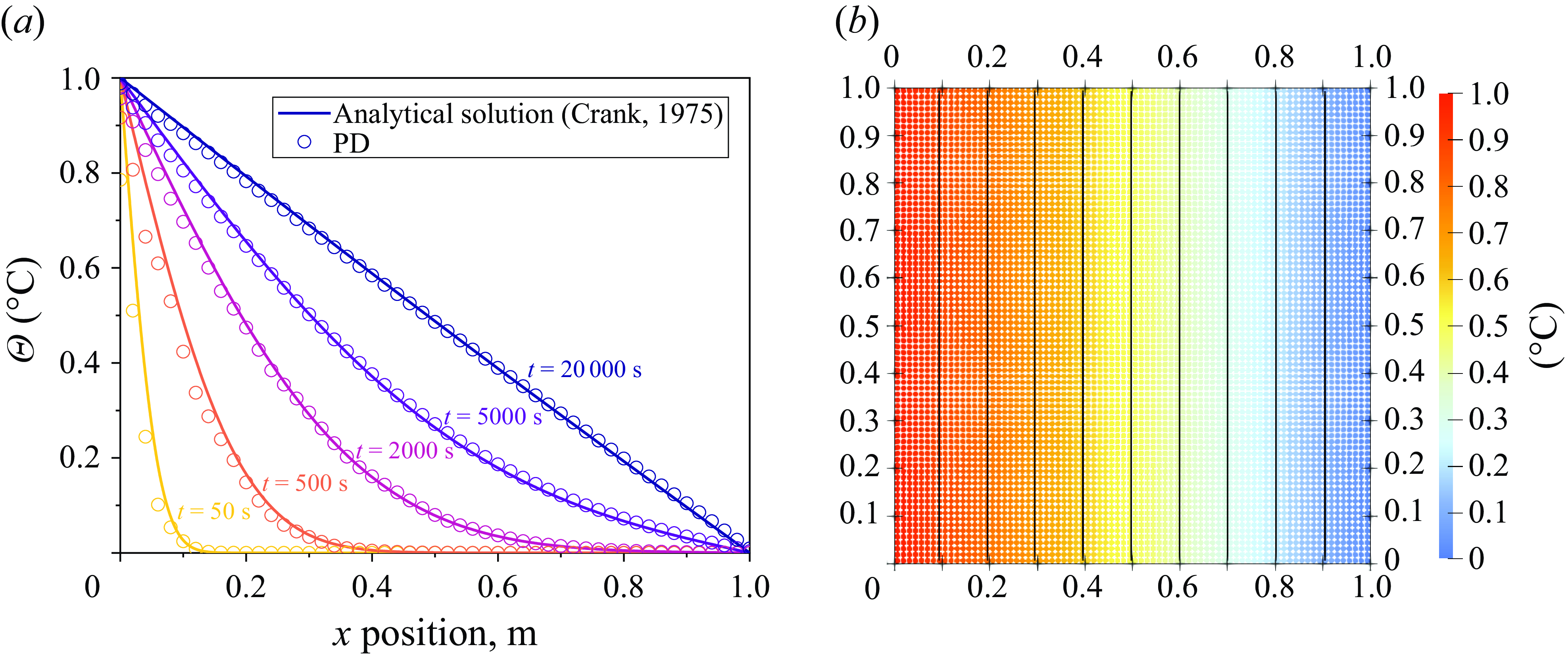
, are shown in figure 6(a). The proposed coupled thermo-hydrodynamic PD method consistently matches well with the analytical solution until reaching the steady state. Figure 6(b) plots the temperature and position at each discretized material point, along with the temperature contour. It can be observed that nearly all the material points remain at their initial positions since there is no external force, and the thermal expansion is not apparent. The temperatures of material points with the same
$(1.0,0.5)$
, are shown in figure 6(a). The proposed coupled thermo-hydrodynamic PD method consistently matches well with the analytical solution until reaching the steady state. Figure 6(b) plots the temperature and position at each discretized material point, along with the temperature contour. It can be observed that nearly all the material points remain at their initial positions since there is no external force, and the thermal expansion is not apparent. The temperatures of material points with the same $x$
position are the same as expected, resulting in a uniformly distributed vertical temperature contour. This example benchmarks the capability of the coupled thermo-hydrodynamic PD model in modelling the heat conduction process.
$x$
position are the same as expected, resulting in a uniformly distributed vertical temperature contour. This example benchmarks the capability of the coupled thermo-hydrodynamic PD model in modelling the heat conduction process.
(a) Comparison between PD results and analytical solution (Crank Reference Crank1975). (b) Temperature contour of simulation results after reaching steady state.
5.2. Natural convection in a closure
In this subsection, the same problem as in § 5.1 is reconsidered by adding the gravity force, which is the driving force of the natural convection phenomenon. De Vahl Davis (Reference De Vahl Davis1983) indicates that the thermal flow becomes turbulent when Ra reaches approximately 106. Therefore, three different Ra values, 103, 104 and 105, are simulated to investigate different patterns of convection. All the other set-ups are the same as adopted in § 5.1.
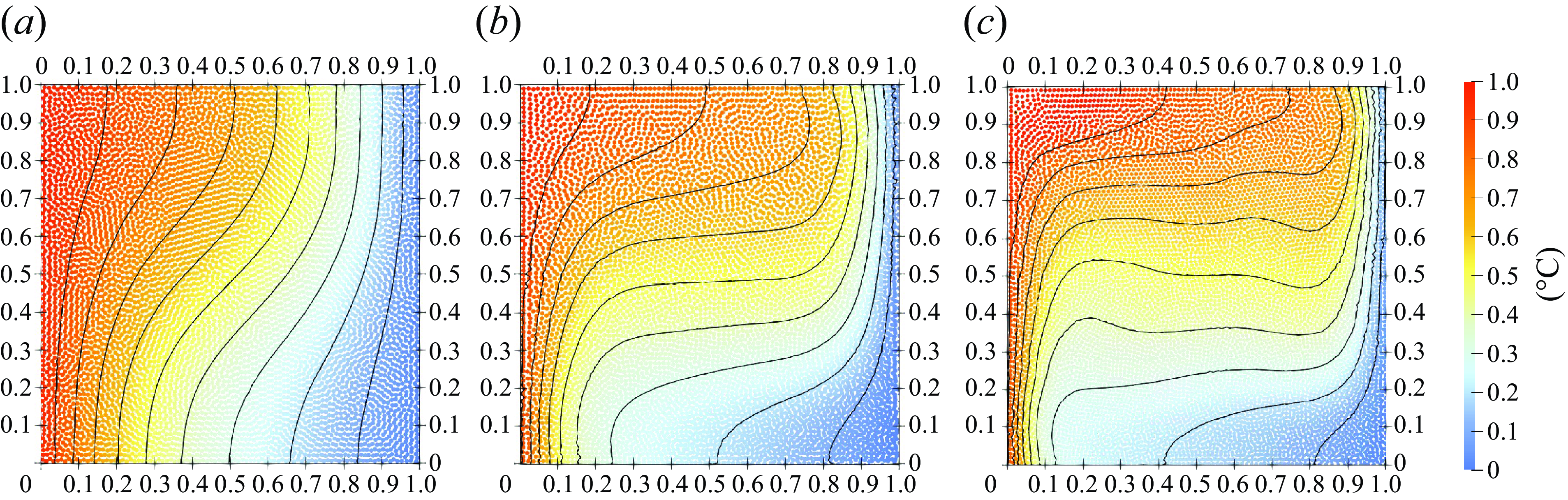
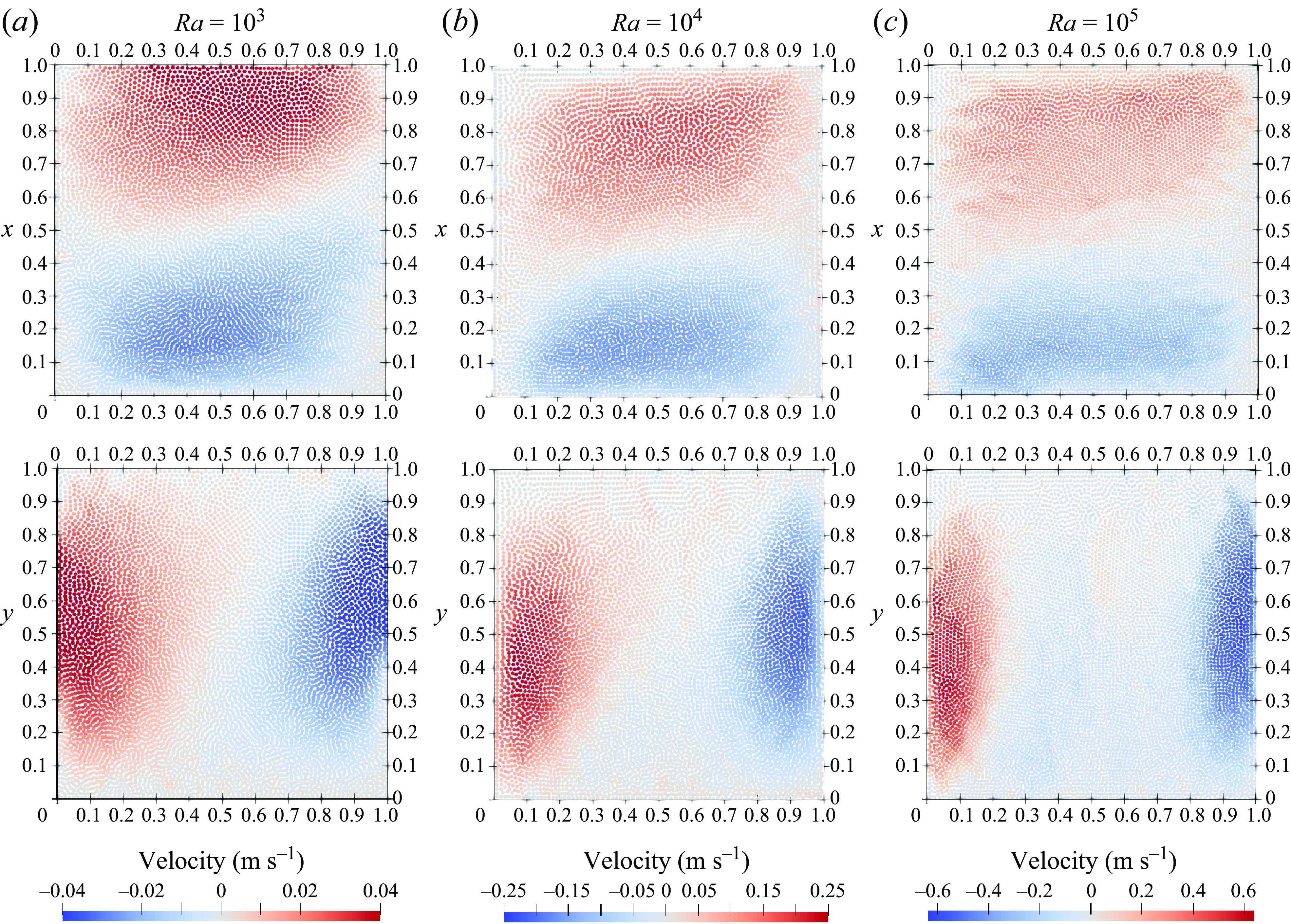
Figure 7 depicts the temperature field for three different cases after reaching the steady state. Different from the results in figure 6(b), the isotherms are all distorted due to the convection process. Owing to the temperature variation, the density at the left-hand and top sides of the cavity would be smaller than the density at the right-hand and bottom sides. Therefore, the density variation further induces a buoyancy force that drives a clockwise circulation within the square cavity. As the Rayleigh number increases, the isotherms become more distorted. This phenomenon indicates that a higher speed flow is generated for higher Ra, as validated by figure 8, in which the velocity distribution in the x and y directions at steady state is shown. For convection with lower Ra, the thermal flow involves a larger part of the material points, while the velocity remains low. As a contrast, with a higher Ra, the velocity of the thermal flow increases significantly, while only the material points near the boundaries participate in the flow. These flow patterns and convective characters are consistent with the literature (Szewc et al. Reference Szewc, Pozorski and Tanière2011; Danis et al. Reference Danis, Orhan and Ecder2013; Gao & Oterkus Reference Gao and Oterkus2019b ). Note that there are oscillations in the velocity field. This is due mainly to the explicit scheme and weakly compressible assumption adopted. The divergence of velocity in (3.4) cannot be guaranteed to be exactly zero in the current scheme. The error may be mitigated by an implicit scheme or explicit incompressible scheme.
Temperature distribution at each material point and temperature contour in the cavity for (a) Ra = 103, (b) Ra = 104, and (c) Ra = 105.
Velocity distribution at each material point for (a) Ra = 103, (b) Ra = 104, and (c) Ra = 105.
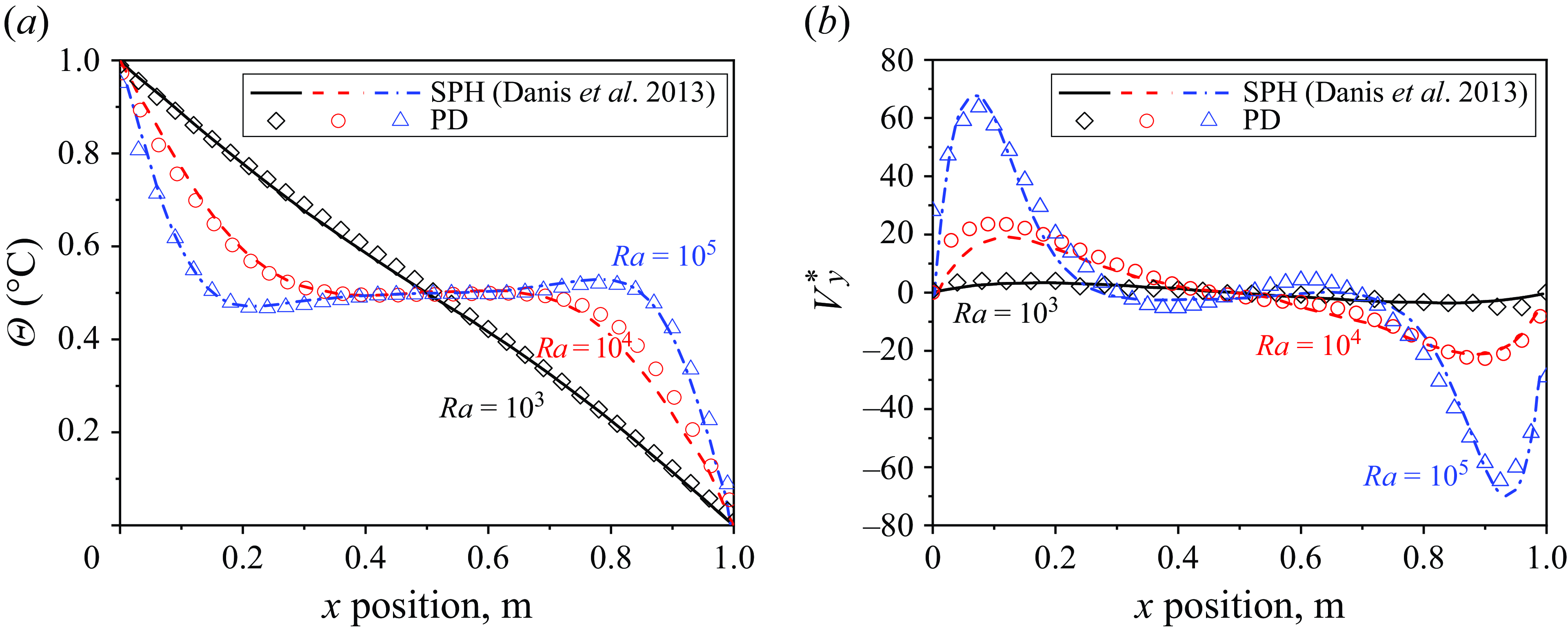
Quantitative comparisons between the proposed PD method and the SPH results along the central horizontal line of the square cavity, i.e. from point (0.0,0.5) to point (1.0,0.5), are shown in figures 9(a,b). When the Rayleigh number is relatively small, the convection is not significant, and the temperature approximately decreases linearly with the x position. As the Rayleigh number increases, the temperature distribution becomes a curve affected by the velocity of material points that boost or hinder the heat transfer. For all Rayleigh numbers, the temperature obtained from the proposed PD method matches well with SPH results. To facilitate a comparison of velocity with Danis et al. (Reference Danis, Orhan and Ecder2013), we normalize the velocity in the same manner as
Comparisons of (a) temperature and (b) normalized velocity in the y direction along the central horizontal line for different Rayleigh numbers.
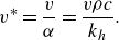 \begin{equation}v^{*}=\frac{v}{\alpha }=\frac{v\rho c}{k_{{h}}}.\end{equation}
As shown in figure 9(b), the peak velocity increases significantly as the Rayleigh number increases, which drives the convection process and makes the temperature contour more distorted. Again, both the trend and value of velocity are consistent with Danis et al. (Reference Danis, Orhan and Ecder2013).
In heat transfer analysis, the Nusselt number is another dimensionless parameter that is widely used to characterize the convective heat transfer between fluid and a solid surface. The local Nusselt number is defined as
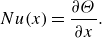 \begin{equation}{Nu}(x)=\frac{\partial \Theta }{\partial x}.\end{equation}
Note that although the boundaries are also modelled by fluid material points herein, it does not affect the validity of the Nusselt number and its definition. The solid boundary can be applied by further developing a coupled THM PD model, which serves as an interesting topic for future research. Figure 10 plots the Nusselt number at the right-hand wall, i.e. from point (1.0,0.0) to point (1.0,1.0), along with SPH results, where good agreements between the two methods are observed for all Rayleigh numbers.
Comparisons of Nusselt numbers at the right-hand wall for (a) Ra = 103, (b) Ra = 104, and (c) Ra = 105.
6. Numerical example and discussions
Another typical natural convection is Rayleigh–Bénard convection, which occurs in a planar horizontal layer of fluid heated from below, as shown in figure 11(a). Different from the cases investigated in §§ 5.1 and 5.2, the gravity force in Rayleigh–Bénard convection is in line with the initial temperature gradient. The Rayleigh–Bénard convection can develop a regular pattern of fluid flow known as a Rayleigh–Bénard cell. The formation of such a convection cell is still attributed to the density difference due to temperature variation and hence buoyancy. The initial movement is the upwelling of less-dense fluid from the warmer bottom layer. The Rayleigh–Bénard convection holds significant importance in various fields. For instance, it is utilized to explain intricate patterns of frost damage in turfgrass (Ackerson, Beier & Martin Reference Ackerson, Beier and Martin2015). In the realm of biochemistry, the Rayleigh–Bénard convection cell is employed for polymerase chain reaction (PCR) processes (Krishnan, Ugaz & Burns Reference Krishnan, Ugaz and Burns2002; Yao, Chen & Ju Reference Yao, Chen and Ju2007), where a steady roll-type convective flow is required to duplicate DNA. In such cases, the temperature gradient between the bottom and top plates plays a crucial role in governing the convection. The Rayleigh number, which is associated with the temperature gradient, must be sufficiently large to initiate convection while avoiding excessive values that could cause turbulent flow. Additionally, without proper cell size design, the possibility of generating multi-roll flows emerges. Consequently, the utilization of numerical simulations offers significant benefits in exploring and understanding these phenomena in greater detail.
Rayleigh–Bénard convection cell: (a) schematic (side view) of an experimental device by Krishnan et al. (Reference Krishnan, Ugaz and Burns2002); (b) sketch map and boundary conditions of PD model.
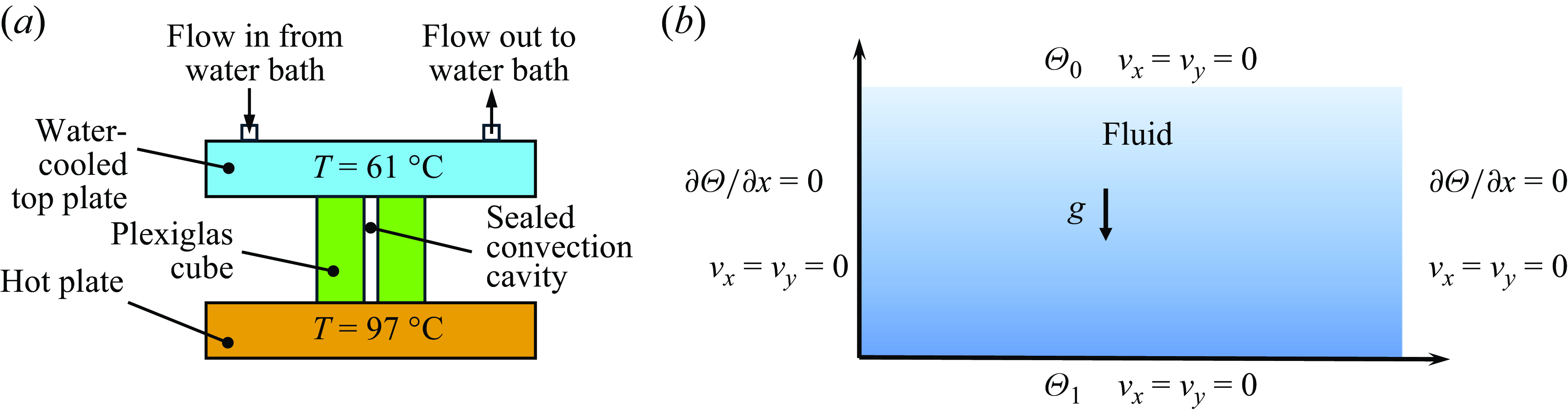
6.1. The PD simulation of Rayleigh–Bénard convection
6.1.1. Roll pattern
Herein, the proposed thermo-hydrodynamic PD model is used to model a Rayleigh–Bénard convection cell as shown in figure 11(b). The right- and left-hand walls of the cell are assumed to be adiabatic. The bottom wall is maintained at a higher temperature denoted as ${\Theta} _{1}$
, while the top wall is subjected to a lower one,
${\Theta} _{1}$
, while the top wall is subjected to a lower one, ${\Theta} _{0}$
. All four surfaces are fixed by setting the velocity in both x and y directions to zero. The properties of the fluid in this case are summarized as follows: density
${\Theta} _{0}$
. All four surfaces are fixed by setting the velocity in both x and y directions to zero. The properties of the fluid in this case are summarized as follows: density $\rho =975$
kg m−3, viscosity
$\rho =975$
kg m−3, viscosity $\mu =0.000377$
Pa s, thermal conductivity
$\mu =0.000377$
Pa s, thermal conductivity $k_{{h}}=6.71$
W m
$k_{{h}}=6.71$
W m $^{-1}$
°C
$^{-1}$
°C $^{-1}$
, specific heat
$^{-1}$
, specific heat $c_{{v}}=4.176$
J kg
$c_{{v}}=4.176$
J kg $^{-1}$
°C
$^{-1}$
°C $^{-1}$
, and thermal expansion coefficient
$^{-1}$
, and thermal expansion coefficient $\beta =0.0005$
°C−1. Note that the properties are selected based on water given in Yao et al. (Reference Yao, Chen and Ju2007), with the specific heat capacity minimized, and the thermal conductivity magnified to obtain a more regular convective pattern. Different temperature differences between the top and bottom walls, and different cell sizes, are used to produce different convective patterns and showcase the capability of the proposed PD method.
$\beta =0.0005$
°C−1. Note that the properties are selected based on water given in Yao et al. (Reference Yao, Chen and Ju2007), with the specific heat capacity minimized, and the thermal conductivity magnified to obtain a more regular convective pattern. Different temperature differences between the top and bottom walls, and different cell sizes, are used to produce different convective patterns and showcase the capability of the proposed PD method.
Temperature distribution at steady state in the cell for: (a) ${\Theta} _{0}=61$
°C and
${\Theta} _{0}=61$
°C and ${\Theta} _{1}=70$
°C; (b)
${\Theta} _{1}=70$
°C; (b) ${\Theta} _{0}=61$
°C and
${\Theta} _{0}=61$
°C and ${\Theta} _{1}=79$
°C; and (c)
${\Theta} _{1}=79$
°C; and (c) ${\Theta} _{0}=61$
°C and
${\Theta} _{0}=61$
°C and ${\Theta} _{1}=97$
°C.
${\Theta} _{1}=97$
°C.
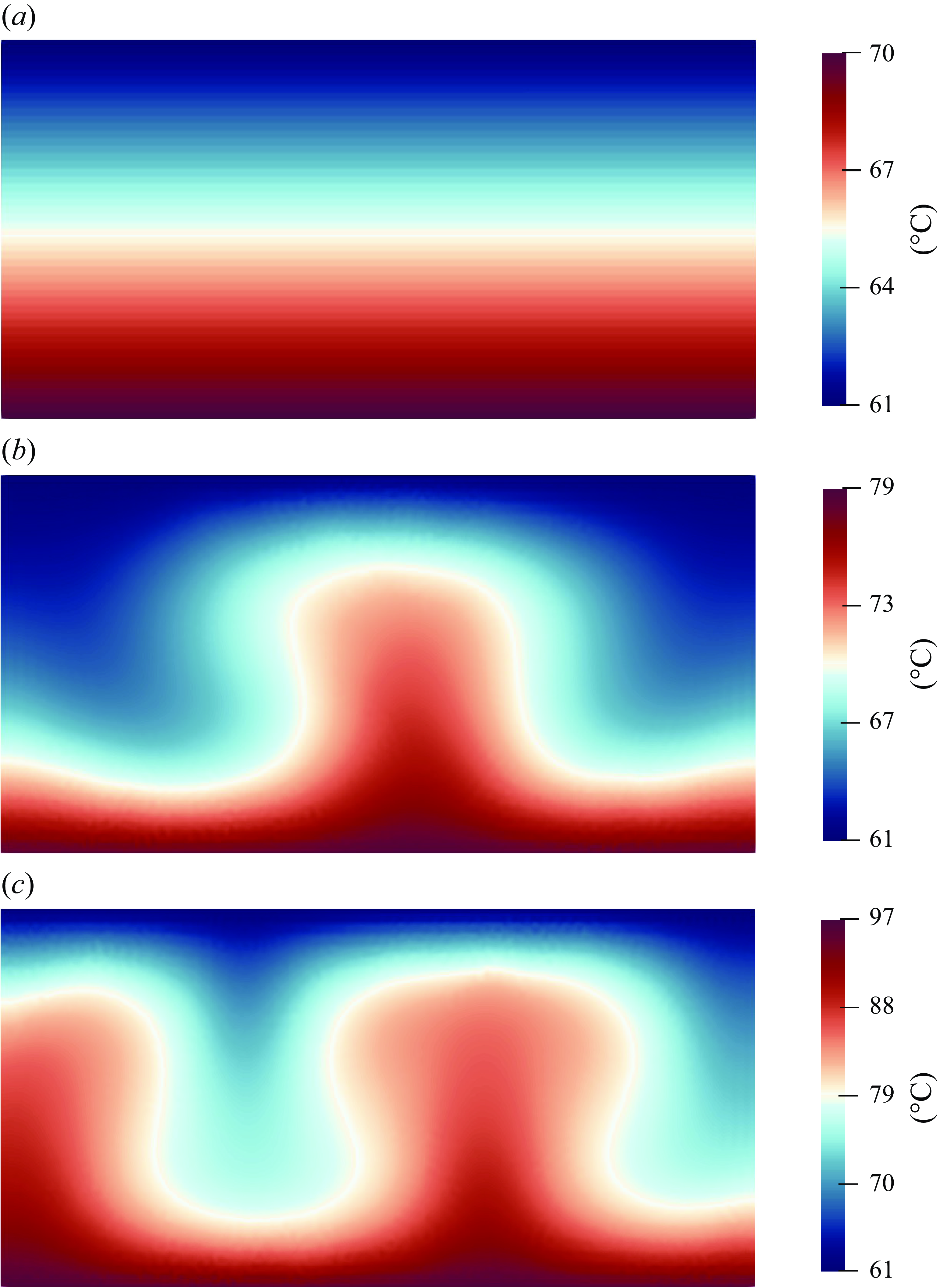
Velocity field at steady state in the cell for: (a) ${\Theta} _{0}=61$
°C and
${\Theta} _{0}=61$
°C and ${\Theta} _{1}=79$
°C; (b)
${\Theta} _{1}=79$
°C; (b) ${\Theta} _{0}=61$
°C and
${\Theta} _{0}=61$
°C and ${\Theta} _{1}=97$
°C. The direction and magnitude of an arrow align with the direction and magnitude of velocity, respectively. The arrows are coloured by density.
${\Theta} _{1}=97$
°C. The direction and magnitude of an arrow align with the direction and magnitude of velocity, respectively. The arrows are coloured by density.
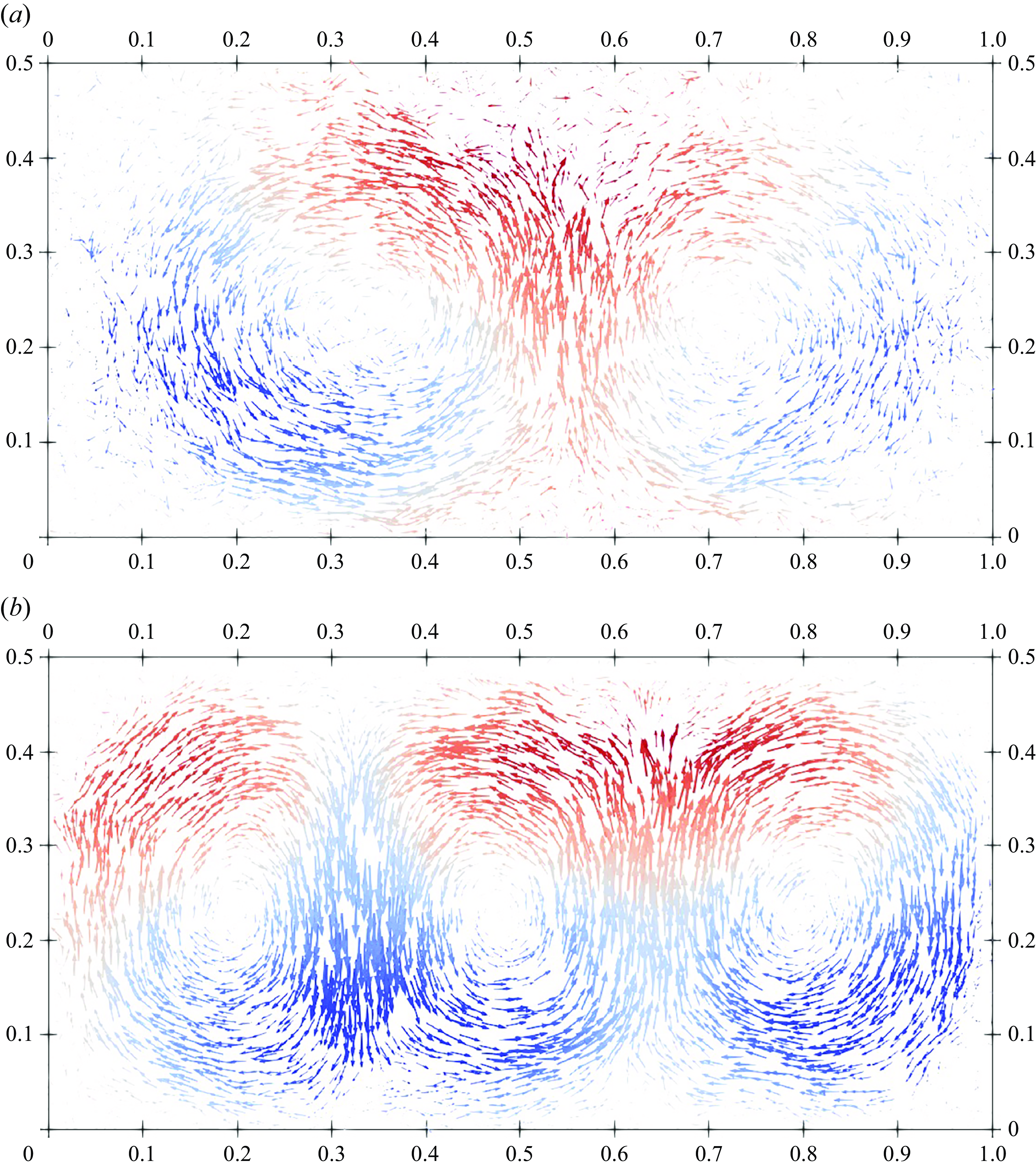
We first investigate a horizontally layered fluid cell with width-to-height ratio 2, as shown in figure 12. If the variation of temperature between the top and bottom plates is minor, then the Rayleigh number is below the critical threshold that would trigger the convection, and the heat transport remains purely conductive. The temperature distributes linearly along the height after reaching the steady state. As the Rayleigh number increases, the pure conductive phase is broken up due to the tendency of upward movement of the heated fluid with lower density. These thermals have a mushroom-like appearance, as indicated by the temperature fronts shown in figures 12(b) and 12(c), which is consistent with the phenomenological model proposed by Howard (Reference Howard and Görtler1966) and the experiment conducted by Sparrow, Husar & Goldstein (Reference Sparrow, Husar and Goldstein1970). Finally, steady double-roll and triple-roll flows are formed for lower and higher Rayleigh number cases, respectively. The velocity of each material point is represented in figure 13 using arrows. The colour map represents the density of corresponding material point and saturates at higher and lower densities (a linear blue–white–red scale represents values from low to high).
It can be observed that the thermal flow initiates from hot fluid with lower densities towards cold regions with higher densities, which once again demonstrates the crucial role of the buoyancy force in natural convection. Such eruption moves colder fluid close to the bottom wall to replace the hot fluid. As the cold fluid is heated through conduction from the wall, it eventually triggers another such eruption. This cyclical process repeats, giving rise to a roll-type flow pattern. The rotation of the flows alternates horizontally between clockwise and anticlockwise. The rolls in figure 13(a) are approximately circular in shape, while those in figure 13(b) appear to be more oval-shaped. This observation suggests a correlation between the Rayleigh number and the shape of the rolls. A higher Rayleigh number corresponds to thermals with increased velocity, which results in a more significant upward movement of the temperature front. Consequently, the rolls tend to take on an elliptical shape, with a longer axis in the vertical direction. In other words, the higher the Rayleigh number, the more elongated or stretched the rolls become vertically. This also explains why three rolls are formed in figures 12(b) and 13(b). The eruption is initiated around the position at $x=0.65$
to form the second and third rolls (from right to left) in figure 13(b). Since both the second and third rolls are elliptical, and there is still enough room in the right-hand side of the cell for the formation of another complete roll, the first roll later is triggered and formed by the downward movement at the right edge of the second roll. Further increase in the temperature applied on the bottom wall results in a turbulent and chaotic flow, which will be explored in detail in later cases. Note that although the geometries of model and boundary conditions are completely symmetric, the steady flow pattern is not. This phenomenon holds true in experiments where spatially random-distributed upward thermals are observed (Sparrow et al. Reference Sparrow, Husar and Goldstein1970; Tritton Reference Tritton2012), and the Rayleigh–Bénard convection is known as one of the typical spontaneous symmetry breaking processes. In terms of numerical modelling, the symmetry of the material points is disrupted after displacements induced by heat conduction and convection. On the other hand, small numerical perturbations may be amplified owing to the non-local nature of the PD theory. To some extent, these simulation results reflect the reality lying in the symmetry breaking process of Rayleigh-Bénard convection.
$x=0.65$
to form the second and third rolls (from right to left) in figure 13(b). Since both the second and third rolls are elliptical, and there is still enough room in the right-hand side of the cell for the formation of another complete roll, the first roll later is triggered and formed by the downward movement at the right edge of the second roll. Further increase in the temperature applied on the bottom wall results in a turbulent and chaotic flow, which will be explored in detail in later cases. Note that although the geometries of model and boundary conditions are completely symmetric, the steady flow pattern is not. This phenomenon holds true in experiments where spatially random-distributed upward thermals are observed (Sparrow et al. Reference Sparrow, Husar and Goldstein1970; Tritton Reference Tritton2012), and the Rayleigh–Bénard convection is known as one of the typical spontaneous symmetry breaking processes. In terms of numerical modelling, the symmetry of the material points is disrupted after displacements induced by heat conduction and convection. On the other hand, small numerical perturbations may be amplified owing to the non-local nature of the PD theory. To some extent, these simulation results reflect the reality lying in the symmetry breaking process of Rayleigh-Bénard convection.
Temperature distribution and roll type within the cell for different width-to-height ratios: (a) 1, (b) 2, (c) 3 and (d) 0.5.
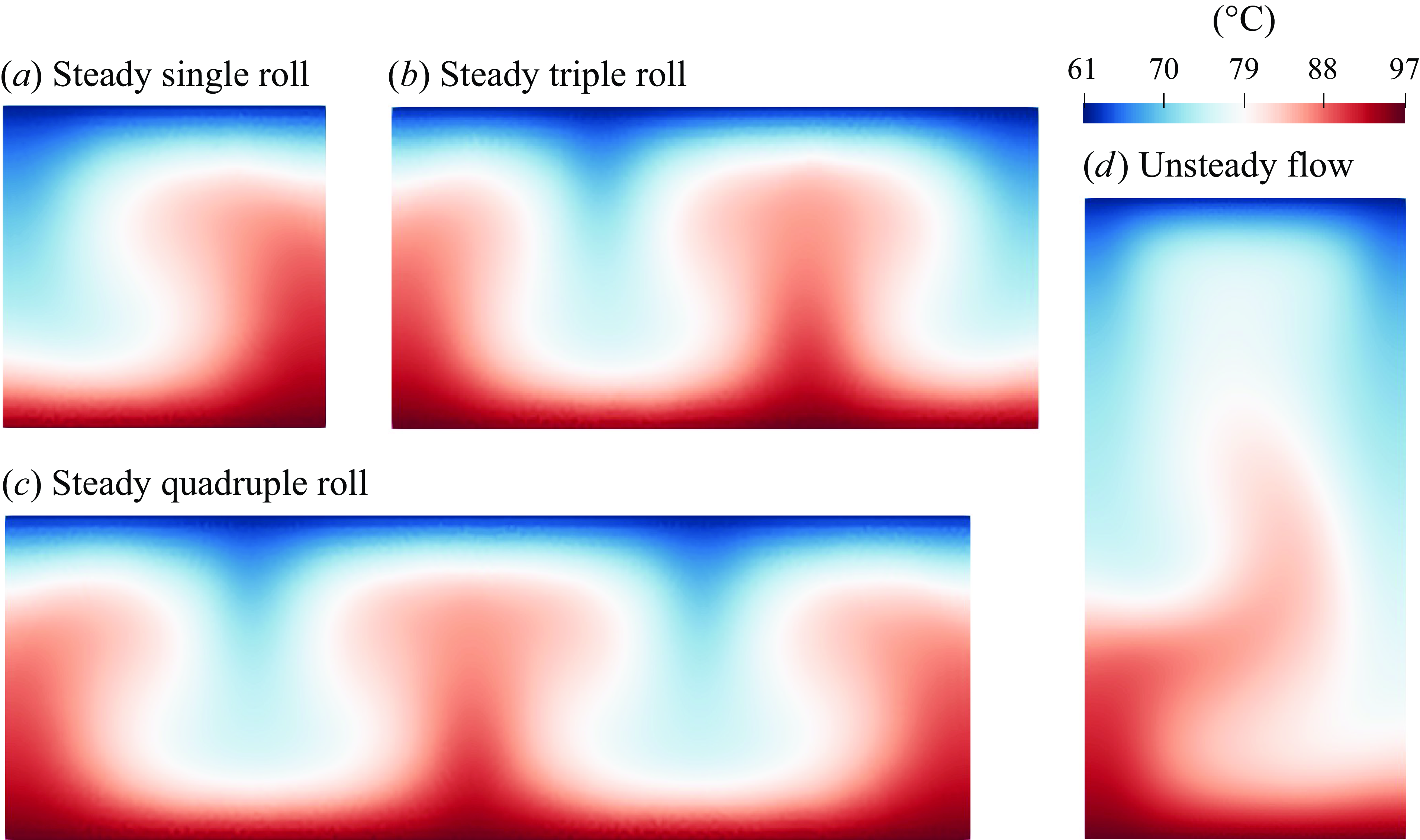

With the temperature of the top and bottom plates kept at 61 °C and 97 °C, respectively, different cell dimensions are adopted to investigate the effects of cell size. The results for width-to-height ratios 1, 2 and 3 are shown in figures 14(a–c). For these three cases, the Rayleigh numbers are the same, and the only differences lie in the width of the cell. The flow at steady state recovers from multi-roll type to single-roll type as the width-to-height ratio decreases, which is in line with the experimental finding by Krishnan et al. (Reference Krishnan, Ugaz and Burns2002). Such a presence of a single steady roll, as depicted in figure 14(a), is advantageous for processes such as PCR. When the width-to-height ratio of the cell is set to 0.5 by doubling the height, the Rayleigh number of the cell in figure 14(d) is eight times of that in the other cases in figures 14(a–c). Consequently, the flow pattern becomes irregular and cannot reach a stable state. The temperature distribution and streamlines at different times are shown in figure 15. The initial thermal flux wanders upwards instead of moving vertically as seen in figures 14(a–c). Subsequently, another new thermal flux emerges and disrupts the original flow. As a result, small-scale disorganized motions coexist alongside the larger-scale circulatory flow, leading to continuous interactions between them. The cell finally forms one single distorted thermal as shown in figures 15(d–f). Although the general shape of the thermal remains similar, this thermal flux still moves continuously with a certain period, akin to the swaying of seaweed in water. This behaviour is more clearly elucidated in figures 15(k,l), where the evolution of streamlines highlights the ongoing movement within the system.
6.1.2. Turbulent thermal flow
To further validate the proposed PD computational method and demonstrate its capability in modelling turbulent thermal flows at high Rayleigh numbers, we numerically reproduce the Rayleigh–Bénard convection experiment conducted by Sparrow et al. (Reference Sparrow, Husar and Goldstein1970), as shown in figure 16. In the experiment, a heating plate of width 9 cm was positioned 8 cm above the bottom of a tank. The dimensions of the tank are width 58 cm and height 40 cm. The tank was filled with water at initial temperature ${\Theta} _{0}=23.6$
°C. The plate was gradually heated to
${\Theta} _{0}=23.6$
°C. The plate was gradually heated to ${\Theta} _{1}=43.1$
°C, and maintained at this temperature. The experimental set-up results in a Rayleigh number up to
${\Theta} _{1}=43.1$
°C, and maintained at this temperature. The experimental set-up results in a Rayleigh number up to $10^{10}$
. For the simulation, we used the actual specific heat capacity and thermal conductivity of water. The experimental observations indicated that the fluid motions and temperature variations on the two sides and below the heating plate were minimal shortly after the heating commenced. Therefore, to optimize computational efficiency, we focus on the region above the heating plate by selecting a simulation domain of width 12 cm and height 30 cm, as illustrated in figure 16. The material point size is set to 0.6 mm, resulting in a total of 104 236 material points.
$10^{10}$
. For the simulation, we used the actual specific heat capacity and thermal conductivity of water. The experimental observations indicated that the fluid motions and temperature variations on the two sides and below the heating plate were minimal shortly after the heating commenced. Therefore, to optimize computational efficiency, we focus on the region above the heating plate by selecting a simulation domain of width 12 cm and height 30 cm, as illustrated in figure 16. The material point size is set to 0.6 mm, resulting in a total of 104 236 material points.
Schematic of experimental set-up in Sparrow et al. (Reference Sparrow, Husar and Goldstein1970) and numerical model.
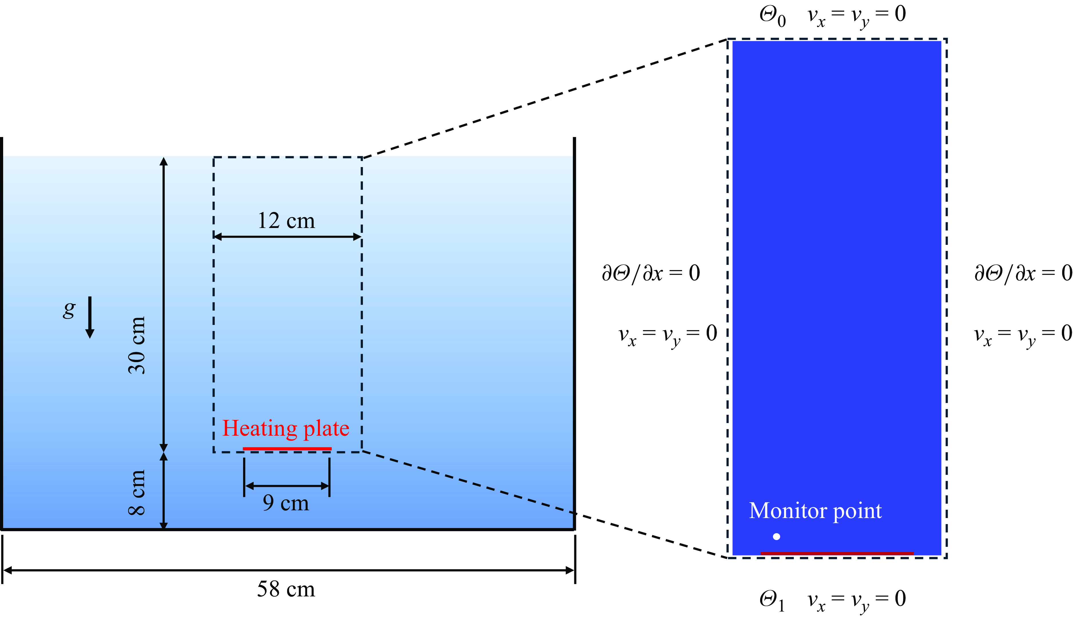
In figure 17, it can be seen that the cellular pattern shown in previous cases is completely gone. These thermals lose their regularity as they ascend. The heights of different thermals are also different. Nevertheless, all thermals manifest as rising columns of fluid, spaced more or less evenly along the expanse of the heated surface. As a thermal ascends through the relatively calm surrounding fluid, its leading edge becomes blunted and folded back, resulting in a nearly semi-spherical cap, and bestowing a mushroom-like appearance upon the thermal. Once these characteristics are established, the locations where the thermals originate appear to be fixed. In other words, subsequent generations of thermals emerge consistently from the same predetermined sites. These characteristics are consistent with the experimental results shown in figure 17(c), where the generations of thermals are in evidence. Figure 18 illustrates the temperature evolution at the monitor point indicated in figure 16. This monitor point is located 0.8 cm above the heating plate, positioned above an active thermal. In the experiment, a thermocouple junction was placed at this location to record temperature changes. The experimental results show that the temperature oscillates with a nearly constant amplitude and a specific frequency, indicating that thermals are generated at almost consistent locations. The periodicity of the oscillations obtained from our numerical results generally aligns well with the experimental recordings. However, the numerical results exhibit slight deviations from strict periodicity and constant amplitude. These discrepancies may be attributed to the smaller simulation domain that was adopted. Another possible reason is that the mesh resolution may be insufficient to fully resolve the interactions between nearby thermals, potentially leading to potential interference between them.
Thermals rising from a heating plate: (a) numerical results obtained from PD; (b) numerical results obtained from SPH; and (c) experimental results (Sparrow et al. Reference Sparrow, Husar and Goldstein1970).
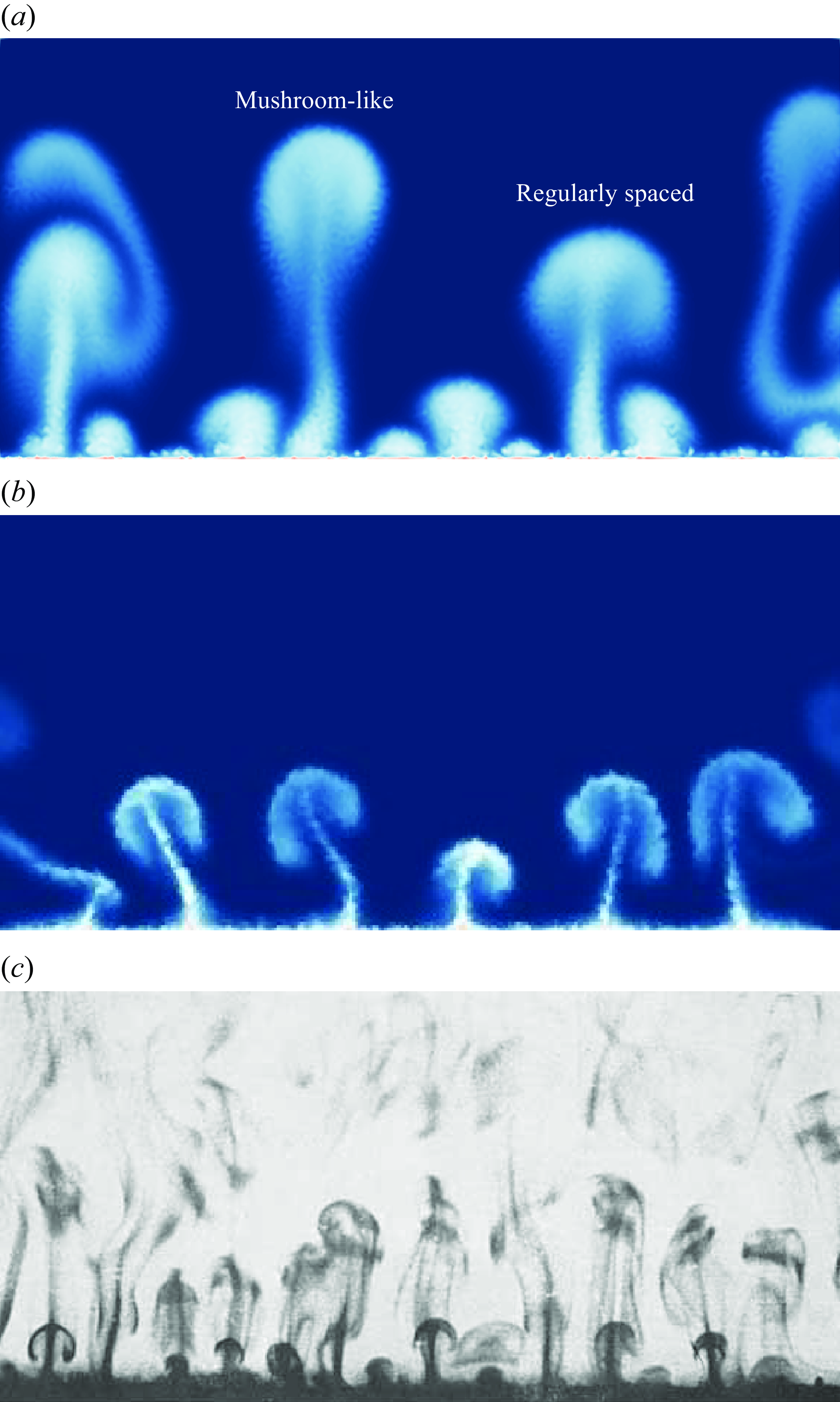
Temperature evolution at a specific point above the heating plate.
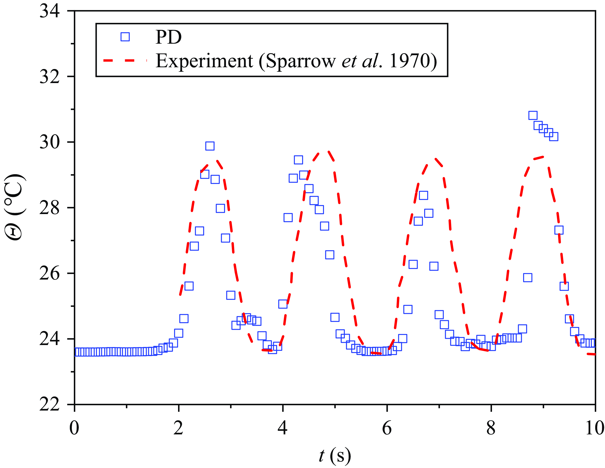
6.2. Discussion: performance and limitations
A key concern regarding the proposed PD method is its computational efficiency. Common fluids, such as water, exhibit low thermal conductivity and high specific heat capacity, which often necessitates significant time to reach steady-state flow or display typical flow patterns. Achieving this with an explicit time integration scheme can lead to substantial computational costs.
To assess the computational efficiency of the proposed PD method, we compare its performance with that of SPH for the turbulent Rayleigh–Bénard convection case. The PD and SPH share several similarities that make them suitable for comparison; both are particle-based methods that rely on interactions between particles. While PD is primarily known for its application in solid mechanics, SPH is widely used for fluid modelling (Feng et al. Reference Feng, Fourtakas, Rogers and Lombardi2021, Reference Feng, Fourtakas, Rogers and Lombardi2024). For this comparison, we reproduce the coupled thermo-hydrodynamic SPH method reported by Reece et al. (Reference Reece, Rogers, Fourtakas and Lind2024). To ensure fair comparison, both PD and SPH employ explicit time integration schemes, identical model set-ups, and the same time step sizes. Additionally, the interaction range for both methods, defined as the horizon in PD and the smoothing length in SPH, is set to three times the particle size. For the turbulent Rayleigh–Bénard convection case, parallel computing is employed using 12 cores of an Intel® Xeon® Gold 6248 @ 3 GHz processor. The numerical result generated by SPH is presented in figure 17(b). Both PD and SPH qualitatively capture the mushroom-shaped thermals. However, based on our current results, SPH appears to produce fewer thermals compared to PD.
Natural convection cases are also simulated using SPH, with computations performed on a single core of the same CPU. The computational times for the different cases, using both PD and SPH, are summarized in table 1. From this table, it can be observed that the computational efficiency of PD is comparable to that of SPH for coupled thermo-hydrodynamic problems when using a single thread. However, PD exhibits lower efficiency than SPH when parallel computing is utilized. This difference can be attributed to several factors. The governing equations in PD, particularly for state-based formulations, are more complex than those in SPH, leading to higher computational overhead. Furthermore, SPH has been extensively used and optimized over several decades, especially in fluid dynamics. As a relatively newer method, PD has not yet benefited from the same level of algorithmic optimization and parallelization efforts as SPH.
Computational time comparison between PD and SPH.
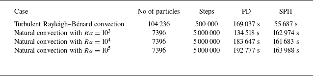
Nevertheless, it is important to acknowledge that the efficiency of particle-based methods, whether PD or SPH, is generally lower than that of element-based methods such as FEM and FVM when modelling internal flows. The primary advantages of particle-based methods lie in their ability to handle free-surface flows and fluid–solid interaction problems with evolving geometries. Unlike element-based methods, which use Eulerian meshes and cannot precisely identify the position of free surfaces within an element, particle-based methods naturally and accurately capture free surfaces. This capability makes them particularly well-suited for problems involving complex interfacial dynamics.
One potential solution to further improve efficiency of PD is to employ an implicit scheme (Bie et al. Reference Bie, Li, Hu and Cui2019), which would allow for a much larger time step. Additionally, the semi-Lagrangian formulation necessitates neighbour searches at each step, which can consume more time than the actual model computations in CPU-based codes. In this context, GPU-accelerated computing (Wang & Yin Reference Wang and Yin2024; Wang et al. Reference Wang, Yin, Wu and Zhu2025) also emerges as a promising approach. While these technical considerations are intriguing, they delve more into the computer science and coding aspects, warranting dedicated future research. The primary focus here is more on the fluid mechanics aspect and the development of the coupled thermo-hydrodynamic formulation within a unified PD framework.
It should be emphasized that the Rayleigh number in the Rayleigh–Bénard convection case reaches up to $10^{10}$
. According to Danis et al. (Reference Danis, Orhan and Ecder2013), thermal flows at such high Rayleigh numbers are inherently turbulent. While the proposed PD method demonstrates the ability to capture typical turbulent thermal flow patterns, its performance for cases with even higher Rayleigh numbers requires further investigation. Additionally, the current implementation does not incorporate a turbulence model. Although the results align reasonably with experimental observations, we anticipate that the accuracy of the simulations could be further enhanced by integrating a turbulence model into the PD framework. This integration would improve the capability of the method to resolve finer-scale turbulent structures and dynamics.
$10^{10}$
. According to Danis et al. (Reference Danis, Orhan and Ecder2013), thermal flows at such high Rayleigh numbers are inherently turbulent. While the proposed PD method demonstrates the ability to capture typical turbulent thermal flow patterns, its performance for cases with even higher Rayleigh numbers requires further investigation. Additionally, the current implementation does not incorporate a turbulence model. Although the results align reasonably with experimental observations, we anticipate that the accuracy of the simulations could be further enhanced by integrating a turbulence model into the PD framework. This integration would improve the capability of the method to resolve finer-scale turbulent structures and dynamics.
Another important aspect of the multi-horizon scheme that warrants exploration is its energy conservation property, which has not been addressed explicitly in previous work (Yang et al. Reference Yang, Zhu and Zhao2024a ). An important assumption made in the present study is that kinetic energy and thermal energy are independent, conserving within their respective horizons. This assumption is fundamental, as fluid flow is driven primarily by internal buoyancy forces, and fluid displacement does not generate or dissipate heat. However, in two-way coupled thermo-hydrodynamic scenarios, such as the plastic flow of liquid metal, where heat generation or dissipation occurs due to fluid movement, ensuring energy conservation in the multi-horizon scheme poses an intriguing challenge that requires further investigation.
7. Conclusion and outlook
This paper presents a new thermo-hydrodynamic model developed within the state-based peridynamics (PD) framework. The semi-Lagrangian PD formulation is adopted for modelling large deformations of fluids. This formulation is extended to non-isothermal conditions by incorporating the energy equation, which governs the heat conduction within the fluids. The energy equation is transformed into a non-local form using non-local gradient and divergence operators to align with the PD formulation. Consequently, multi-physics analysis involving fluid flow with heat transfer can be conducted effectively within the framework. To mitigate the numerical oscillations in thermal fields and to reduce computational costs, a multi-horizon scheme is proposed for coupled thermo-hydrodynamic modelling, where a smaller horizon is adopted for the thermal field (i.e. temperature), and a larger horizon is used for the flow field (i.e. velocity, acceleration). The proposed method is benchmarked against a pure conduction problem and a classical natural convection problem in a closed cavity. Further applications demonstrate the capabilities of the coupled PD method in capturing complex thermal flow patterns, including steady roll-type flows and turbulent mushroom-like thermals, as evidenced by experiments. Quantitative comparisons between the numerical results and recorded experimental data on periodicity and frequency of turbulent thermal generation further validated the proposed method.
The proposed computational method paves the way for the future development of a unified framework for computational modelling of coupled THM processes for both solids and fluids, particularly in scenarios where evolving discontinuities in solids play a critical role. Such scenarios are commonly encountered in nature and engineering applications. For instance, magma-driven fracturing (Spence & Turcotte Reference Spence and Turcotte1985; Taddeucci et al. Reference Taddeucci, Cimarelli, Alatorre‐Ibargüengoitia, Delgado-Granados, Andronico, Del Bello, Scarlato and Di Stefano2021) in crustal rocks serves as a typical example. Similarly, in geothermal energy exploitation, cool water is injected into hot dry rock to create a more interconnected fracture network. In these contexts, the intricate interplays between mechanical and thermal fracturing, heat conduction and convection in and across different phases, as well as fluid flow, must all be considered. The proposed PD method for fluid modelling can be integrated seamlessly with existing thermo-mechanical PD solid models, such as the one developed by Yang et al. (Reference Yang, Zhu and Zhao2024a ), which is capable of modelling heat transfer in solids as well as fracture initiation and propagation. Since both fluid and solid components can be modelled within a single particle-based framework, there is no need to explicitly define the fluid–solid interface. This represents a significant advantage when addressing complex, evolving geometries in fluid–structure interaction problems. Furthermore, coupling PD fluid and solid models does not require specialized techniques. A straightforward fictitious point method (Yang et al. Reference Yang, Zhu and Zhao2024b ) can be employed to complete the horizons of interacting solid and fluid material points. This unified framework can be extended further to incorporate phase change processes between fluid and solid, enabling the modelling and interpretation of many intriguing phenomena in geoscience, such as igneous processes and rainfall- or temperature-induced fracture initiation and propagation in glaciers.
Acknowledgements
The authors acknowledge valuable comments and suggestions from the anonymous reviewers. C.Y. acknowledges support from the Hong Kong PhD Fellowship Scheme funded by the Research Grants Council of Hong Kong.
Funding
The study was financially supported by the National Science Foundation of China (J.Z., grant no. 11972030), Research Grants Council of Hong Kong (J.Z., grant nos GRF project 16212724, CRF project C7082-22G, TRS projects T22-607/24N and T22-606/23-R), and a JSPS KAKENHI Grant (F.Z., grant no. 23K13403).
Declaration of interests
The authors report no conflict of interest.
Author contributions
C.Y.: writing – original draft, writing – review & editing, visualization, validation, software, methodology, investigation, formal analysis, data curation. J.Z.: writing – review & editing, supervision, conceptualization, project administration, methodology, funding acquisition. F.Z.: writing – review & editing, methodology, software, conceptualization, funding acquisition. R.F.: validation, data curation.
Data availability statement
Data will be made available upon request.


 Open access