


1. Introduction
Natural convection is important in many technological applications owing to the passive character of the resulting heat transfer. It can change widely depending on the geometry of the flow system, with inclined slots representing one of the fundamental reference configurations (Bergman et al. Reference Bergman, Lavine, Incropera and DeWitt2017). Inclined slots are of interest in the development of energy-efficient building ventilation systems (Wong & Heryanto Reference Wong and Heryanto2004; Mortensen, Walker & Sherman Reference Mortensen, Walker and Sherman2011; Li, Yeoh & Timchenko Reference Li, Yeoh and Timchenko2015), passive cooling devices (Naylor, Floryan & Tarasuk Reference Naylor, Floryan and Tarasuk1991; Straatman, Tarasuk & Floryan Reference Straatman, Tarasuk and Floryan1993; Straatman et al. Reference Straatman, Naylor, Tarasuk and Floryan1994; Novak & Floryan Reference Novak and Floryan1995; Shahin & Floryan Reference Shahin and Floryan1999; Andreozzi, Buonomo & Manca Reference Andreozzi, Buonomo and Manca2005; Mehiris et al. Reference Mehiris, Ameziani, Rahli, Bouhadef and Bennacer2017), in predicting fire propagation (Song et al. Reference Song, Huang, Kuenzer, Zhu, Jiang, Pan and Zhong2020) and in the removal of smoke from structures (Putnam Reference Putnam1882).
Structured convection, which results from the use of spatial heating patterns, possesses some intriguing properties. It has been extensively studied in horizontal slots, but scant information is available about inclined slots. Structured convection should not be confused with the ubiquitous Rayleigh–Bénard convection (Bénard Reference Bénard1900; Rayleigh Reference Rayleigh1916) which occurs only in horizontal slots and when critical conditions are met – these onset conditions do not depend on the Prandtl number Pr. Patterned heating is different as it creates convection rolls regardless of the heating intensity and the intensity of the resulting movement as a function of Pr (Hossain & Floryan Reference Hossain and Floryan2013). Patterned heating may lead to secondary convection, but the heating intensity required for its onset strongly depends on the heating wavenumber  $\alpha $ (Hossain & Floryan Reference Hossain and Floryan2013). The wavenumber of the secondary convection is locked in with the heating wavenumber when $\alpha = O(1)$, but in the case of short heating wavelength $(\alpha \to \infty )$, the wavenumber of the secondary convection approaches the critical Rayleigh–Bénard value. The form of the secondary convection changes significantly over the range of heating wavenumbers and it is possible to have frustrated systems as well as responses in the form of soliton lattices (Hossain & Floryan Reference Hossain and Floryan2013, Reference Hossain and Floryan2022; Nixon et al. Reference Nixon, Ronen, Friesem and Davidson2013). There is an up/down convection symmetry for heating applied at the upper and lower plates (Hossain & Floryan Reference Hossain and Floryan2014, Reference Hossain and Floryan2015a). When a forced convection component is added, an increase in the flow Reynolds number leads to rapid transition from rolls to travelling waves (Hossain & Floryan Reference Hossain and Floryan2015b). The use of staggered heating has been reported as providing superior heat transfer in turbulent convection when compared with uniform heating (Li et al. Reference Li, Yeoh and Timchenko2015).
The presence of grooves in the slots leads to particularly interesting system responses, with the sparse available data limited to horizontal slots only. Corrugations on one of the isothermal plates results in convection regardless of the heating intensity, with the form of convection dictated by the groove geometry, and the intensity being a function of the Prandtl number (Abtahi & Floryan Reference Abtahi and Floryan2017a). A combination of such grooves with heating patterns activates the pattern interaction effect (Floryan & Inasawa Reference Floryan and Inasawa2021) which creates thermal streaming (Abtahi & Floryan Reference Abtahi and Floryan2017b, Reference Abtahi and Floryan2018; Inasawa, Hara & Floryan Reference Inasawa, Hara and Floryan2021).
The use of patterned heating in channels has been investigated as a method for flow control. It was shown that such heating reduces pressure losses in horizontal channels (Hossain, Floryan & Floryan Reference Hossain, Floryan and Floryan2012; Floryan & Floryan Reference Floryan and Floryan2015; Hossain & Floryan Reference Hossain and Floryan2016; Inasawa, Taneda & Floryan Reference Inasawa, Taneda and Floryan2019). When channels are grooved the pattern interaction effect can significantly reduce pressure losses, but this relies on carefully chosen relative positions of the grooves and heating pattern (Hossain & Floryan Reference Hossain and Floryan2020).
The present study represents the first analysis of laminar natural convection in inclined slots exposed to patterned heating and our objective is to develop a basic understanding of such convection. We limit our interests to small heating rates to avoid transition to a secondary state. The remainder of the paper is organized as follows. In § 2, we provide a description of the model problem. Section 3 discusses convection driven by heating applied at the lower plate: in particular we look at purely periodic heating, the effect of the Prandtl number and what happens when we have combined periodic/uniform heating. Section 4 is devoted to the problem when both plates are heated while § 5 provides a short summary of the main conclusions. The main results described in §§ 3 and 4 are numerical in nature, and further understanding of the properties of the convection is provided in a few supplementary appendices. In these analytical sections we focus on both long-wavelength and short-scale heating patterns as well as describing the properties of weak convection.
2. Problem formulation
Consider a slot formed by smooth plates and inclined with respect to gravity as shown in figure 1. The slot is supposed to contain a Boussinesq fluid while the gravitational acceleration acts downwards.
Schematic diagram of the flow system.

The plates are subjected to spatial heating patterns. Of course, there is an almost limitless set of patterns that could be proposed, but as our aim is to develop some elementary understanding of the problem, we focus on the simplest pattern fully characterized by a single Fourier mode (although we relax this in § 4.3). Hence, we suppose that the two plates are held at temperatures given by
 \begin{gather}y ={-} 1:{\theta _L}(x) = R{a_{uni,L}} + {\textstyle{1 \over 2}}R{a_{p,L}}\cos (\alpha x),\end{gather}
 \begin{gather}y ={+} 1:{\theta _U}(x) = R{a_{uni,U}} + {\textstyle{1 \over 2}}R{a_{p,U}}\cos (\alpha x + \varOmega );\end{gather}
Here, the subscripts L and U denote the lower and upper plates,  $\alpha $ stands for the heating wavenumber and $\lambda = 2{{\rm \pi} }/\alpha $ is the heating wavelength. The relative temperature is defined to be $\theta = T - {T_L}$ scaled on $\kappa \nu /(g\varGamma {h^3})$; here T denotes the temperature, the lower plate temperature ${T_L}$ is adopted as the reference temperature while g, $\varGamma $, $\nu $ and $\kappa $ are the gravitational acceleration, the thermal expansion coefficient, the kinematic viscosity and the thermal diffusivity respectively.
It is noted that the applied heating profiles comprise uniform and periodic parts. The former is encapsulated by the two Rayleigh numbers  $R{a_{uni,L}} = g\varGamma {h^3}{\theta _{uni,L}}/(\kappa \nu )$ and $R{a_{uni,U}} = g\varGamma {h^3}{\theta _{uni,U}}/(\kappa \nu )$, where ${\theta _{uni,L}}$ and ${\theta _{uni,U}}$ are the uniform temperature components. The two parameters $R{a_{p,L}} = g\varGamma {h^3}{\theta _{p,L}}/(\kappa \nu )$ and $R{a_{p,U}} = g\varGamma {h^3}{\theta _{p,U}}/(\kappa \nu )$ are the lower and upper periodic Rayleigh numbers which measure the amplitudes of the modulations; here, ${\theta _{p,L}}$ and ${\theta _{p,U}}$ are the differences between the maximum and minimum of the lower and upper periodic temperature components, respectively. Lastly, we note that, while the periodic parts of the two heating profiles have identical wavelengths, we allow them to be offset by a prescribed phase difference.
Convection in the slot is described by the continuity, Navier–Stokes and energy equations. When expressed in dimensionless forms these may be cast as
 \begin{gather}u\frac{{\partial u}}{{\partial x}} + v\frac{{\partial u}}{{\partial y}} ={-} \frac{{\partial p}}{{\partial x}} + {\nabla ^2}u + P{r^{ - 1}}\theta \sin \beta ,\quad \frac{{\partial u}}{{\partial x}} + \frac{{\partial v}}{{\partial y}} = 0,\end{gather}
 \begin{gather}u\frac{{\partial v}}{{\partial x}} + v\frac{{\partial v}}{{\partial y}} ={-} \frac{{\partial p}}{{\partial y}} + {\nabla ^2}v + P{r^{ - 1}} \theta \cos \beta ,\quad u\frac{{\partial \theta }}{{\partial x}} + v\frac{{\partial \theta }}{{\partial y}} = P{r^{ - 1}}{\nabla ^2}\theta ,\end{gather}
where  $(u,v)$ are the velocity components in the (x, y) directions, respectively, scaled on ${U_v} = \nu /h$, which is adopted as the velocity scale. Furthermore, here, p is the pressure scaled on $\rho U_\nu ^2$, $\beta $ denotes the inclination angle to the horizontal and $Pr = \nu /\kappa $ is the Prandtl number. The associated boundary conditions at the lower and upper plates have the form
 \begin{gather}u(y ={-} 1) = u(y = 1) =
0, v(y ={-} 1) = v(y = 1) = 0,\nonumber\\ \quad\quad \theta
(y ={-} 1)=\theta_{L}(x),\quad \theta (y = 1)=\theta_{U}(x),\end{gather}
\begin{gather}u(y ={-} 1) = u(y = 1) =
0, v(y ={-} 1) = v(y = 1) = 0,\nonumber\\ \quad\quad \theta
(y ={-} 1)=\theta_{L}(x),\quad \theta (y = 1)=\theta_{U}(x),\end{gather}
and are supplemented by the periodicity conditions in the x-direction. Since there is no externally imposed mean pressure gradient acting along the slot, it is necessary to add the zero mean pressure gradient constraint in the form
 \begin{equation}{\left. {\frac{{\partial p}}{{\partial x}}} \right|_{mean}} \equiv {\lambda ^{ - 1}}\int_{{x_0}}^{{x_0} + \lambda } {\frac{{\partial p}}{{\partial} x}}\,{\partial x} = 0,\end{equation}
where the subscript  $mean$ refers to the mean value and $\lambda = 2{{\rm \pi} }/\alpha $ is the wavelength of the heating. The system (2.1)–(2.5) was solved numerically by expressing the velocity components in terms of a streamfunction $\psi $ defined in the usual manner so that $u = \partial \psi /\partial y$ and $v ={-} \partial \psi /\partial x$. This enables the pressure to be eliminated from the governing system and the remaining unknowns were written in the form of Fourier expansions in the x-direction together with Chebyshev expansions in the y-direction. Details of the underlying algorithm and testing of its accuracy can be found in Hossain et al. (Reference Hossain, Floryan and Floryan2012). The pressure field was normalized by bringing the mean value of its periodic component to zero. The net axial flow rate Q and the average Nusselt number $N{u_{av}}$ were then defined to be
 \begin{gather}Q = {\left[ {\int_{ - 1}^{ + 1} {u(x,y)\,\textrm{d}y} } \right]_{mean}},\end{gather}
 \begin{gather}N{u_{av}} ={-} {\lambda ^{ - 1}}\int_{{x_0}}^{{x_0} + \lambda } {{{\left. {\frac{{\partial \theta }}{{\partial y}}} \right|}_{y ={-} 1}}\,\textrm{d}\kern0.06em x} .\end{gather}
Written in this way a positive value of  $N{u_{av}}$ corresponds to the situation in which the lower plate delivers energy to the fluid. Moreover, the shear forces acting on the fluid at the lower and upper plates are given by
 \begin{align}\begin{gathered}{F_L} = {\lambda ^{ - 1}}\int_0^\lambda {{\sigma _{xv,L}}\,\textrm{d}\kern0.06em x} ={-} {\lambda ^{ - 1}}\int_0^\lambda {{{\left. {\frac{{\partial u}}{{\partial y}}} \right|}_{y ={-} 1}}\,\textrm{d}\kern0.06em x} ,\nonumber\\ {F_U} = {\lambda ^{ - 1}}\int_0^\lambda {{\sigma _{xv,U}}\,\textrm{d}\kern0.06em x} = {\lambda ^{ - 1}}\int_0^\lambda {{{\left. {\frac{{\partial u}}{{\partial y}}} \right|}_{y ={+} 1}}\,\textrm{d}\kern0.06em x} ,\end{gathered}\end{align}
while the total (buoyancy) body force per unit length is
 \begin{equation}{F_{xb}} = {\lambda ^{ - 1}}P{r^{ - 1}}\sin \beta \int_{ - 1}^1 {\int_0^\lambda {\theta \,\textrm{d}\kern0.06em x\,\textrm{d}y} } \quad \textrm{and}\quad {F_{yb}} = {\lambda ^{ - 1}}P{r^{ - 1}}\cos \beta \int_{ - 1}^1 {\int_0^\lambda {\theta \,\textrm{d}\kern0.06em x\,\textrm{d}y} } ,\end{equation}
where  ${F_{xb}}$ and ${F_{yb}}$ denote the x- and y-components.
3. Heating of the lower plate
We begin our investigation by examining the convection that arises when only the lower plate is heated so that  $R{a_{uni,U}} = R{a_{p,U}} = 0$. In passing, we remark that in the subsequent calculations results are presented for air (Pr = 0.71) unless otherwise noted. We limit our interest to $R{a_{p,L}} < 1400$ unless demonstration of special flow properties requires use of more intense heating.
3.1. Periodic heating
We first assume that the lower plate is subject to a purely periodic heating, i.e.  $R{a_{uni,L}} = 0$, which means that the thermal boundary conditions take the form
 \begin{equation}{\theta _L}(x) = {\textstyle{1 \over 2}}R{a_{p,L}} \textrm{cos(}\alpha x\textrm{),}\quad {\theta _U}(x) = 0.\end{equation}
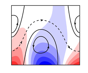
Fluid motion is driven by the buoyancy force and variations of its x- and y-components as functions of the inclination angle are illustrated in figure 2. The x-component (acting along the slot) vanishes if the slot is either horizontal or vertical but is non-zero for all intermediate inclinations. The y-component (acting across the slot) is greatest when the slot is horizontal and as  $\beta $ grows so this component diminishes until it is zero when the slot is vertical. These forces lead to a vastly different patterns of convection, as shown in figure 3, which illustrates the flow and temperature fields when the slot is either horizontal, inclined or vertical.
Variation of the x- and y-components of the total body force  $({F_{xb}},{F_{yb}})$ and the shear forces acting on the fluid at the lower $({F_L})$ and upper $({F_U})$ plates as functions of the inclination angle $\beta $ for $\alpha = 1.5$, and (a) $R{a_{p,L}} = 400$ and (b) $R{a_{p,L}} = 1200$.

The flow and the temperature fields for  $R{a_{p,L}} = 400$, $\alpha = 1.5$ and (a) $\beta = 0$, (b) $\beta = {{\rm \pi} }/4$ and (c) $\beta = {{\rm \pi} }/2$. Solid lines identify streamlines within the separation bubbles while dashed lines identify streamlines within the stream tube. The temperature was normalized with ${\theta _{max}} = R{a_{p,L}}/2$. Solid arrows show direction of gravity and different components of the buoyancy force.

Periodic heating of the horizontal slot produces convection in the form of pairs of counter-rotating rolls (see figure 3a). Fluid rises above the hot spots and draws replacement fluid along the plate from its sides; this eventually forms closed rolls with borders that overlap with the hot and cold spots. Fluid elements move within the convective rolls with no net movement in the horizontal direction. Periodic heating in a vertical slot also forms counter-rotating rolls with no net movement in the vertical (see figure 3c) but the mechanics of the process is somewhat different. Now hot fluid adjacent to the heated section of the plate moves upwards while cold fluid near the cooler section of the plate moves downwards. These streams collide and are forced to turn towards the interior of the slot, thereby creating counter-rotating rolls. The interface between adjacent rolls meets the plate where its temperature is zero. We remark on the existence of the y-component of the buoyancy force when the slot inclined away from the vertical.
Flow in an inclined slot is qualitatively different in character. The fact that the slot is inclined breaks symmetries that are present in the horizontal or vertical positions, thereby producing a net flow along the channel. The flow topology consists of a family of counter-rotating rolls which is supplemented by a stream tube that meanders between them and which carries the fluid in the upward direction (see figure 3b). This phenomenon can be explained as the result of formation a non-zero component of the buoyancy force that acts along the slot. One can interpret this process as a hot plume impacting and bouncing off an oblique upper plate. Some of the fluid is permanently trapped inside the rolls while the remainder travels along the slot. The cumulative net flow is a function of both the inclination angle and the heating intensity, and it seems that the upper rolls significantly weaken as the intensity of heating increases (see figure 4). Indeed, we note that the upper rolls were completely washed away once  $R{a_{p,L}} > 2200$ (for the combination of flow parameters used in figure 4).
The flow and the temperature fields for  $\alpha = 1.5$, $\beta = 0.166{{\rm \pi} }$ and the four values of $R{a_{p,L}} = (a)\ 400, (b)\ 1000, (c)\ 1600\ \textrm{and}\ (d)\ 2200$. Solid lines identify streamlines within the separation bubbles while dashed lines identify streamlines within the stream tube. Temperature was normalized with ${\theta _{max}} = R{a_{p,L}}/2$.

The strength of the convective movement and its dependence on the inclination angle and the applied heating can be ascertained by considering the nature of the flow rate Q (see figure 5a). There is no net flow when the slot is horizontal as the buoyancy force is directed across the slot. Similarly, there is also no net flow in a vertical channel as the mean buoyancy force along the slot is zero. The flow rate increases with  $R{a_{p,L}}$ and the value of $\beta $ at which the flow rate is greatest does depends on $R{a_{p,L}}$. At relatively small values of $R{a_{p,L}}$ the critical inclination angle for greatest Q is approximately $\beta = {{\rm \pi} }/4$ but as $R{a_{p,L}}$ increases, this angle decreases and reaches $\beta \approx 0.15{{\rm \pi} }$ when $R{a_{p,L}} = 1400$ (see the inset of figure 5a). The maximum of Q correlates well with the maximum of the x-component of the buoyancy force ${F_{xb}}$ (see figure 2). The heat transfer shows a somewhat different dependence; it is greatest when $\beta = 0$ and decreases to zero when $\beta = {{\rm \pi} }/2$. We point out that the variations in the heat transfer are similar to those of the transverse component of the buoyancy force ${F_{yb}}$ (see figure 2). The mean fluid temperature increases above the base value in horizontal and inclined slots but $N{u_{av}} = 0$ when the slot is vertical (see figure 5b). We also notice that at relatively modest values of $R{a_{p,L}}$ the value of $N{u_{av}}$ decreases monotonically with $\beta $ but this behaviour ceases at larger $R{a_{p,L}}$. These properties are in accord with the analytical solutions developed for the long- and short-wavelength limits (see the appendices).
Variations of (a) the flow rate Q and (b) the average Nusselt number  $N{u_{av}}$ as functions of the inclination angle $\beta $ for $\alpha = 1.5$ and for selected values of $R{a_{p,L}}$. The inset graph in figure 5(a) shows the variation of the angle ${\beta _{max}}$ corresponding to the maximum flow rate as a function of $R{a_{p,L}}$.

More information concerning the velocity and temperature fields can be gleaned by examining these quantities at some carefully chosen streamwise locations. We consider the four stations  $x = 0$, $x = \lambda /4$, $x = \lambda /2$ and $x = 3\lambda /4$; the first and third of these are hot and cold spots, respectively, while at the other two locations the wall temperature is zero. The hot and cold spots coincide with the borders between adjacent rolls in horizontal slots while the points of zero temperature are where the fluid movement is strongest. The situation is exactly reversed in vertical slots. The distributions of the u-velocity and the temperature profiles displayed in figure 6 help illustrate the effects of the inclination angle. The thermal structures are barely affected at all by the convection in a vertical slot at $x = \lambda /4\ \textrm{and}\ 3\lambda /4$ (see figure 6c); the changes are still minor but noticeable in horizontal slots (see the distributions at $x = 0,\lambda /2$ in figure 6a) whilst significant changes can be observed in inclined slots (see figure 6b). The velocity distributions show no net flow at $x = \lambda /4\ \textrm{and}\ 3\lambda /4$ in horizontal slots (figure 6a) and at $x = 0,\lambda /2$ in vertical slots (figure 6c). By way of contrast, large changes in velocity distributions between different test locations are observed in the case of inclined slots (figure 6b).
Distribution of the x-velocity component u (solid lines) and the temperature  $\theta $ (dashed lines) as functions of y for $R{a_{p,L}} = 400, \alpha = 1.5$ and (a) $\beta = 0$, (b) $\beta = {{\rm \pi} }/4$ and (c) $\beta = {{\rm \pi} }/2, \varOmega = {{\rm \pi} }$. Temperature was normalized with ${\theta _{max}} = R{a_{p,L}}/2$. The thin dotted horizontal line in (b) identifies the zero level in u and $\theta $.

The distributions of shear stresses acting on the fluid at each plate are illustrated in figure 7. The zero-stress points coincide with the hot and cold spots when the slot is horizontal and with the zero-temperature points when the slot is vertical. The average shear stress is zero on each plate for each of these two slot orientations. The situation is markedly different for inclined slots as then the positions of the zero-stress points shift between the two extreme positions discussed above. The two plates experience different average stresses with the larger value associated with the heated plate; note that the sum of these two stresses balance the x-component of the total buoyancy force  ${F_{xb}}$.
Distributions of shear stress acting on the fluid at (a) the lower and (b) the upper plates for  ${Ra_{p,L}} = 400$, $\alpha = 1.5$.

The forms of Q and  $N{u_{av}}$ as functions of $R{a_{p,L}}$ are shown in figure 8 for various inclination angles $\beta $. At relatively modest values of the Rayleigh number, it is found that both Q and $N{u_{av}}$ are proportional to $Ra_{p,L}^2$ irrespective of the inclination angle. As $R{a_{p,L}}$ grows there are signs of saturation leading to a reduction of the growth of these quantities observed once $R{a_{p,L}}$ exceeds approximately 500, with the saturation of Q being more pronounced and occurring much earlier for the near-vertical slot position (see figure 8a). The structure of the flow at modest values of $R{a_{p,L}}$ is explained analytically in Appendix C.
Variations of (a) the flow rate Q and (b) the average Nusselt number  $N{u_{av}}$ as functions of the periodic Rayleigh number $R{a_{p,L}}$ for $\alpha = 1.5$.

A calculation of the effects of the heating wavenumber  $\alpha $ on Q and $N{u_{av}}$ suggests that the maximum flow rate and the maximum heat flow occur when $\alpha \approx 1.5$; the values of the wavenumbers at which these maximums are achieved seem to be insensitive to the inclination angle (see figure 9). Both Q and $N{u_{av}}$ appear to be proportional to ${\alpha ^2}$ in the long-wavelength limit $\alpha \to 0$ and to decrease like ${\alpha ^{ - 3}}$ in the limit of $\alpha \to \infty $. These predictions can be confirmed by suitable asymptotic analyses which are outlined in Appendices A and B, respectively.
Variations of (a) the flow rate Q and (b) the average Nusselt number  $N{u_{av}}$ as functions of the heating wavenumber $\alpha $ for $R{a_{p,L}} = 400$.

The convection adopts some interesting characteristics as the wavenumber  $\alpha $ grows, as illustrated in figures 10 and 11. The temperature variations are confined to a thin boundary layer adjacent to the heated plate while the convective movement takes the form of counter-rotating rolls confined to the same zone, at least when the slot is either horizontal or vertical (see figures 10a and 10c). The fluid motion is qualitatively different when the slot is inclined as then it occupies the whole slot (see figures 10b and 11). In this case, the heating creates spatial modulations within the boundary layer which drives a unidirectional flow across the remainder of the slot. Theoretical analysis of the flow structures is relegated to Appendix B.
The flow and temperature fields for  $R{a_{p,L}} = 400$, $\alpha = 10$, and for the three inclination angles (a) $\beta = 0$, (b) $\beta = {{\rm \pi} }/4$ and (c) $\beta = {{\rm \pi} }/2$. Solid lines identify streamlines within the separation bubbles while dashed lines identify streamlines within the stream tube. The temperature was normalized with ${\theta _{max}} = R{a_{p,L}}/2$.

The profiles of the u-velocity component (solid lines) and the temperature  $\theta $ (dashed lines) as functions of y for $R{a_{p,L}} = 400, \alpha = 10$ at four streamwise locations and the three inclinations angles (a) $\beta = 0$, (b) $\beta = {{\rm \pi} }/4$ and (c) $\beta = {{\rm \pi} }/2$. Again, the temperature was normalized with ${\theta _{max}} = R{a_{p,L}}/2$.

3.2. Effects of Prandtl number
All the results discussed so far pertain to the Prandtl number  $Pr = 0.71$. Some additional data displayed in figure 12 suggest that the flow rate Q decreases with an increase of Pr and that this quantity may be proportional to $P{r^{ - 1}}$ for $Pr > 1$ regardless of the inclination angle. On the other hand, the average Nusselt number appears to increase with Pr before approaching a limiting $\beta $-dependent value when $Pr$ exceeds approximately 3.
Variations of (a) the flow rate Q and (b) the average Nusselt number  $N{u_{av}}$ as functions of Pr for $\alpha = 1.5$.

In an effort to explain the underlying large Pr structure, we seek solutions that take the forms
 \begin{align}\begin{gathered}u = P{r^{ - 1}}\hat{U}(x,y) + \cdots ,\quad v = P{r^{ - 1}}\hat{V}(x,y) + \cdots ,\nonumber\\ p = P{r^{ - 1}}\hat{P}(x,y) + \cdots \textrm{,}\quad \theta = \hat{\varTheta }(x,y) + \cdots .\end{gathered}\end{align}
The substitution of these in the continuity, Navier–Stokes and energy equations give rise to the leading-order balances
 \begin{align}\begin{gathered} 0 ={-} {\hat{P}_x} + {\hat{U}_{xx}} + {\hat{U}_{yy}} + \hat{\varTheta }\sin \beta ,0 ={-} {\hat{P}_y} + {\hat{V}_{xx}} + {\hat{V}_{yy}} + \hat{\varTheta }\cos \beta ,\nonumber\\ \quad 0 = {\hat{U}_x} + {\hat{V}_y},\quad \hat{U}{\hat{\varTheta }_x} + \hat{V}{\hat{\varTheta }_y} = {\hat{\varTheta }_{xx}} + {\hat{\varTheta }_{yy}}.\end{gathered}\end{align}
Unfortunately, these equations are only slightly simpler than the full system, with only the nonlinear terms in the two momentum equations removed. A complete account of the large  $Pr$ problem would necessitate a numerical solution of these minimally reduced equations; this is not particularly illuminating so is not discussed further here. Nevertheless, we can be confident that, in the large Prandtl number limit, the Nusselt number remains $O(1)$ while the mass flux diminishes proportional to $O(P{r^{ - 1}})$, as suggested in figure 12.
3.3. Combined uniform heating/cooling and periodic heating
To generalize the results thus far, we supplement the periodic heating of the lower plate with a uniform component. Consequently, the appropriate thermal boundary conditions become
 \begin{equation}{\theta _L}(x) = R{a_{uni, L}} + {\textstyle{1 \over 2}} R{a_{p,L}}\textrm{cos(}\alpha x\textrm{)},\quad {\theta _U}(x) = 0.\end{equation}
We point out that, if we turn off the periodic component of the heating, the associated temperature and velocity fields, the flow rate and the average Nusselt number are
 \begin{align}\begin{gathered}\theta = \frac{1}{2}R{a_{uni,L}}(1 - y),\quad u = \frac{1}{{12Pr}}R{a_{uni,L}}\sin (\beta )({y^2} - 1)(y - 3),\nonumber\\ Q = \frac{1}{{3Pr}}R{a_{uni,L}}\sin (\beta ),\quad N{u_{av}} = \frac{1}{2}R{a_{uni,L}}.\end{gathered}\end{align}
There is no longitudinal flow in a horizontal slot – such flow only appears when the slot is inclined. Sinusoidal heating alone generates an upward flow, as discussed previously. The addition of a small component of uniform heating leads to an increase in the upward flow (see figure 13). There is an optimal value of  $\beta $ at which the flow rate is largest and further increase in the inclination angle then reduces the flow rate (see figure 13a). Computations suggest that the optimal angle approaches ${{\rm \pi} }/2$ as $R{a_{uni,L}}$ increases. The dependence of the average Nusselt number on $\beta $ is very reminiscent of its form in the purely periodic case (see figure 5b) with the curves displaced upwards by a distance equal to $N{u_{av}}$ for uniform heating (see figure 13b).
Illustration of the effects of uniform heating; (a) the variation of the flow rate Q and (b) the average Nusselt number  $N{u_{av}}$ for various levels of uniform heating as functions of the inclination angle $\beta $ when $\alpha = 1.5$. Solid lines denote results for combined uniform and periodic heating with $R{a_{p,L}} = 200$. Dashed lines indicate the reference results for a purely uniform heating $(R{a_{p,L}} = 0)$.

The effects of uniform cooling are illustrated in figure 14. Enhanced cooling tends to suppress the flow rate and reverses its direction for larger inclinations angles, as shown in figure 14(a). It also decreases the average Nusselt number and changes the direction of heat flow if  $\beta $ is sufficiently large, as depicted in figure 14(b).
Illustrations of the effects of uniform cooling − variations of (a) the flow rate Q and (b) the average Nusselt number  $N{u_{av}}$ for a selection of uniform cooling values as functions of the inclination angle $\beta $ for $\alpha = 1.5$. Dashed lines provide reference results for a purely uniform cooling. Solid lines denote results for the combined uniform cooling and periodic heating with $R{a_{p,L}} = 200$.

3.4. Periodic heating of the upper plate
We briefly mention the situation where the heating is switched from the lower to the upper plate. In the purely periodic case
 \begin{equation}{\theta _L}(x) = 0,\quad {\theta _U}(x) = {\textstyle{1 \over 2}}R{a_{p,U}}\cos (\alpha x),\end{equation}
and some sample results are shown in figure 15. The mechanics of the flow is akin to that seen previously for the heating of the lower plate in as much that is there is no net flow within horizontal or vertical slots (see figures 15a and 15c) but there is a non-zero downward flow when the slot is inclined (see figure 15b).
The flow and temperature fields for  $R{a_{p,U}} = 400$, $\alpha = 1.5$ and three inclinations angles (a) $\beta = 0$, (b) $\beta = {{\rm \pi} }/4$ and (c) $\beta = {{\rm \pi} }/2$. Solid lines identify streamlines within the separation bubbles while dashed lines identify streamlines within the stream tube. The temperature was normalized with ${\theta _{max}} = R{a_{p,U}}/2$. Thick arrows show direction of gravity and different components of the buoyancy force.

The similarity in the flow patterns depending on whether the upper or lower plate is heated is perhaps not surprising. Indeed, it is relatively simple to show that the governing systems for the two problems are closely related. If we take the problem of a heated lower plate with  $R{a_{p,L}} = B$ and $R{a_{p,U}} = 0$ and then make the transformation $R{a_{p,L}} \to 0$, $R{a_{p,U}} \to B$, $u \to - U$, $v \to - V$, $p \to P$, $\theta \to - \varTheta $, $x \to - X + {{\rm \pi} }$, $y \to - Y$, we find that the underlying equations are unchanged but the thermal boundary conditions are reversed in sign. The consequence is that the flux Q switches sign while $N{u_{av}}$ is unaltered. Given this relationship between the two cases, there is no need to dwell further on the case of upper plate heating as all the interesting properties can be inferred directly from the results of the computations when it is the lower plate that is heated.
4. Sinusoidal heating of both plates
We next consider the problem when the heating of both plates gives rise to the pattern interaction problem. The uniform heating is removed thereby leading to thermal boundary conditions of the form
 \begin{equation}{\theta _L}(x) = {\textstyle{1 \over 2}}R{a_{p,L}}\cos (\alpha x),\quad {\theta _U}(x) = {\textstyle{1 \over 2}}R{a_{p,U}}\cos (\alpha x + \varOmega ),\end{equation}
i.e. both patterns are characterized by the same wavenumber  $\alpha $ while their relative position is specified in terms of a phase difference $\varOmega $. In general, we allow the two heating intensities to be different, but perform our initial calculations with them being the same.
4.1. Identical heating intensities
Our first set of results relates to the case when  $R{a_{p,L}} = R{a_{p,U}}$. There is a wide variety of possible flow patterns depending on the slot inclination $\beta $ and the phase shift $\varOmega $, and a sample of the possibilities is shown in figure 16. We can see an example of a layer of straight rolls (figures 16a,i), a layer of inclined rolls (figure 16b,d–f,h) and two layers of rolls (figure 16c,g).
The flow and temperature fields for  $R{a_{p,L}} = R{a_{p,U}} = 200$, $\alpha = 1.5$ and various combinations of the inclination angle $\beta$ and phase offset $\varOmega $. The temperature was normalized with ${\theta _{max}} = R{a_{p,U}}/2$; (a) $\beta = 0,\varOmega = 0$, (b) $\beta = 0,\varOmega = {{\rm \pi} }/2$, (c) $\beta = 0 , \omega = pi$, (d) $\beta = {{\rm \pi} }/4,\varOmega = 0$, (e) $\beta = {{\rm \pi} }/4,\varOmega = {{\rm \pi} }/2$, (f) $\beta = {{\rm \pi} }/4,\varOmega = {{\rm \pi} }$, (g) $\beta = {{\rm \pi} }/2,\varOmega = 0$, (h) $\beta = {{\rm \pi} }/2,\varOmega = {{\rm \pi} }/2$ and (i) $\beta = {{\rm \pi} }/2,\varOmega = {{\rm \pi} }$.

None of these configurations appear to produce a net flow along the slot. If this is the case, then it ought to be provable from the governing system of equations. If we take the system (2.3) with  $R{a_{p,L}} = R{a_{p,U}}$ then we can transform the variables according to $u \to - U$, $v \to - V$, $p \to P$, $\theta \to - \varTheta $, $x \to - X + {{\rm \pi} } - \varOmega $ and $y \to - Y$. With these changes it can be verified that the governing equations are unaltered whilst the boundary conditions are also preserved. The upshot is that the x-independent mean component of the streamwise velocity u, call it ${u_m}(y)$, has the property that ${u_m}(y) ={-} {u_m}( - y)$ and hence it is an odd function of y. Since the integral of any odd-valued function over the interval $- 1 \le y \le 1$ necessarily vanishes, the flow rate $Q = 0$ for any values of $\alpha ,\beta $ and $\varOmega $. Using an analogous argument, it can be concluded that the mean part of the thermal profile is also an odd-valued function of y, but this does not have any implication for the value of the average Nusselt number.
4.2. Different heating intensities
We next turn to comment on the possibilities when the heating intensities are different. Some sample flow and temperature fields are illustrated in figure 17 when it is the lower plate that is heated more strongly. The convection patterns are dominated by more intense heating with the net upward flow rate persisting even in vertical slots.
The flow and temperature fields when  $R{a_{p,L}} = 200,R{a_{p,U}} = 100$, $\alpha = 1.5$ for a selection of slot inclinations $\beta $ and phase shifts $\varOmega $. The temperature was normalized so that ${\theta _{max}} = R{a_{p,L}}/2$; (a) $\beta = 0,\varOmega = {{\rm \pi} }/2$, (b) $\beta = {{\rm \pi} }/4,\varOmega = {{\rm \pi} }/2$, (c) $\beta = {{\rm \pi} }/2,\varOmega = {{\rm \pi} }/2$, (d) $\beta = 0,\varOmega = 3{{\rm \pi} }/2$, (e) $\beta = {{\rm \pi} }/4,\varOmega = 3{{\rm \pi} }/2$ and (f) $\beta = {{\rm \pi} }/2,\varOmega = 3{{\rm \pi} }/2$.

The dependence of the flow rate on the phase difference  $\varOmega $ is sketched in figure 18. Two cases are considered; in the first the upper plate is cooler than the lower one while the second set of results relates to the case when the situation is reversed. The identity of the hotter plate seems to dictate the direction of the fluid movement; the flow is predominantly upwards when the lower plate is hotter and downwards otherwise. There is no net flow rate when the slot is horizontal. It is possible to get a net flow rate either up or down within a vertical slot − this depends on the phase difference between the two heating patterns. The flow rate can also change significantly in an inclined slot as the phase difference is varied and this is illustrated in figure 19. It is possible to change the flow rate by up to 50 % by changing the phase difference, with the largest change generally occurring when $\beta \approx {{\rm \pi} }/4$.
The variation of the flow rate Q as a function of the phase difference  $\varOmega $ when $R{a_{p,L}} = 200$, $\alpha = 1.5$. In (a) the lower plate is hotter with ${Ra_{p,U}} = 100$; in (b) the upper plate is the warmer $(R{a_{p,U}} = 300)$.

The variations of the flow rate Q as a function of  $\beta $ when ${Ra_{p,L}} = 200$, $\alpha = 1.5$. In (a) $R{a_{p,U}} = 100$ while in (b) $R{a_{p,U}} = 300$. Dashed lines show the values of Q generated by heating one plate only.

The role played by the heating wavenumber is explored in figure 20. These results demonstrate a large sensitivity of Q to changes of  $\varOmega $ for $\alpha = O(1)$ but this effect is moderated and is accompanied by a rapid decrease in the flow rate in both the small and large $\alpha $ limits. The Nusselt number retains a delicate dependence on $\varOmega $ when the wavenumber is not large, and the direction of the heat flow can change direction under certain conditions.
The variations of (a) the flow rate Q and (b, c) the average Nusselt number  $N{u_{av}}$ as functions of the heating wavenumber $\alpha $ when $\beta = {{\rm \pi} }/4$. In (a) $R{a_{p,L}} = 200$, $R{a_{p,U}} = 100$ (left y-axis) together with $R{a_{p,L}} = 200$, $R{a_{p,U}} = 300$ (right y-axis). In (b) $R{a_{p,L}} = 200$, $R{a_{p,U}} = 100$ while in (c) $R{a_{p,L}} = 200$, $R{a_{p,U}} = 300$. Dashed lines in (b,c) denote a change in sign.

A vertical slot represents a special case for which the unequal heating of the sides generates a net flow. The size of this effect can be significant for O(1) values of  $\alpha $ but rapidly decreases to zero as $\alpha \to \infty $, as illustrated in figure 21.
Variations in (a) the flow rate Q and (b) the average Nusselt number  $N{u_{av}}$ in a vertical slot as functions of the heating wavenumber $\alpha $. Blue curves correspond to $R{a_{p,L}} = 200$, $R{a_{p,U}} = 100$, $\varOmega = {{\rm \pi} }/2$; red curves correspond to $R{a_{p,L}} = 200$, $R{a_{p,U}} = 300$, $\varOmega = {{\rm \pi} }/2$.

We comment that an analysis of long-wavelength heating shows that the flow rate
 \begin{equation}Q = \frac{1}{{18\,900Pr}}{\alpha ^2}(Ra_{p,L}^2 - Ra_{p,U}^2)\sin (2\beta ),\end{equation}
does not depend on the phase difference and its direction depends on which plate is heated the more strongly. Details of the solution can be found in Appendix A. The form of  $N{u_{av}}$ is given by
 \begin{equation}N{u_{av}} ={-} {\textstyle{1 \over {720}}}\alpha R{a_{p,L}}R{a_{p,U}}\sin (\varOmega )\sin (\beta ),\end{equation}
and shows a sensitivity to  $\varOmega $; moreover, there is a linear reduction of $N{u_{av}}$ with $\alpha $ when $\beta \ne 0$ and $\sin \varOmega \ne 0$. If the slot is horizontal, or if the phase shift $\varOmega = 0$ or ${{\rm \pi} }$, then $N{u_{av}}$ decreases proportional to ${\alpha ^2}$.
An analysis of the short-wavelength heating limit demonstrates that
 \begin{equation}Q \!=\! \frac{1}{{1536Pr}}{\alpha ^{ - 3}}(Ra_{p,L}^2 - Ra_{p,U}^2)\sin (2\beta )\quad \textrm{and}\quad N{u_{av}} = \frac{1}{{512}}{\alpha ^{ - 3}}(Ra_{p,L}^2 \!+\! Ra_{p,U}^2)\cos (\beta ).\end{equation}
Details of the solution can be found in Appendix B.
4.3. Different heating wavenumbers
For completeness we briefly consider the modifications to the picture that emerge should the two prescribed heating wavenumbers be different. This then is an example of a pattern interaction problem (Floryan & Inasawa Reference Floryan and Inasawa2021). To focus the presentation, consider patterns at the lower and upper plates characterized by wavenumbers  ${\alpha _L}$ and ${\alpha _U}$, respectively. This gives rise to thermal boundary conditions of the form
 \begin{equation}{\theta _L}( - 1) = \frac{{R{a_{p,L}}}}{2}\cos ({\alpha _L}x),\quad {\theta _U}(1) = \frac{{R{a_{p,L}}}}{2}\cos ({\alpha _U}x + \varOmega ).\end{equation}
Here, for simplicity, we have assumed that both plates are exposed to the same heating intensity  $R{a_{P,L}}$. The expected form of the system response depends on the ratio of the two wavenumbers $CI = {\alpha _L}/{\alpha _U}$, which we shall henceforth refer to as the commensurability index. Rational values of $CI$ lead to periodic system responses with wavelengths which can vary by several orders of magnitude, and these are so-called commensurable states. On the other hand, irrational values give rise to aperiodic responses. If one denotes the system wavelength by ${\lambda _s}$, clearly this needs to be an integer multiple of the individual wavelengths $2{{\rm \pi} }/{\alpha _L}$ and $2{{\rm \pi} }/{\alpha _U}$.
An illustrative system performance is depicted in figure 22 where the lower wavenumber was set as  ${\alpha _L} = 2$ while the upper wavenumber was allowed to take one of several prescribed values. Only results for the simplest systems are described here. When $CI = 1$, so that ${\alpha _L} = {\alpha _U}$, we recover the situation described in § 4.1, which is unable to generate net flow regardless of the slot inclination angle. When $CI = 0.5$, so that the upper heating wavelength is twice that of the lower, the situation changes. The resulting flow and temperature fields (when $\varOmega = {{\rm \pi} }/4$) are shown in figure 23(a) and further computations show that a net flow is produced that can be directed either to the left or to the right, depending on the relative positioning of the heating patterns. As the offset $\varOmega $ is adjusted, it appears that the corresponding $N{u_{av}}$ undergoes much smaller changes in value than is the case when ${\alpha _L} = {\alpha _U}$. In the opposite situation $CI = 2$, when the upper heating wavelength is now one half of the lower, some typical flow and temperature patterns are now presented in figure 23(b). The resulting flow rate is now much larger and always seems to be directed upwards with a magnitude that only varies slightly with $\varOmega $.
Variation of (a) the flow rate Q and (b) the average Nusselt number  $N{u_{av}}$ as functions of the phase shift $\varOmega $ for three values of the commensurability index $CI = 0.5,\, 1,\, 2$, and for $\beta = {{\rm \pi} }/4$, $R{a_{p,L}} = R{a_{p,U}} = 200$. In all cases the wavenumber at the lower wall is ${\alpha _L} = 2$.

The flow and temperature fields when (a)  $CI = 0.5$ and (b) $CI = 2$. All results correspond to the values $\beta = {{\rm \pi} }/4, R{a_{p,L}} = R{a_{p,U}} = 200$ and $\varOmega = {{\rm \pi} }/4$. The solid lines identify streamlines within the separation bubbles while dashed lines identify streamlines within the stream tube. The temperature was normalized with ${\theta _{max}} = R{a_{p,L}}/2$. The lower wall wavenumber is ${\alpha _L} = 2$ in both cases.

These limited results are enough to demonstrate that a wide range of possible behaviours of the flow system arises when it is subject to heating governed at two wavenumbers. Our intention here is simply to point out the wealth of possible phenomena rather than to prosecute an exhaustive analysis. Our calculations seem to suggest that it is the component of the heating pattern associated with the longer wavelength that prevails and dictates direction of the net flow. One may also look at the responses from a symmetry point of view. We have seen that no net flow is created when both plates are subject to the same heating at the same wavenumber but the symmetry inherent within this situation is destroyed when the two intensities are different; of course, the one-wall heating result discussed in § 3 is just an extreme example of this effect. The symmetry can also be lost should the two heating intensities be kept equal but different heating wavenumbers employed. It is not straightforward to infer the likely properties of the flow and requires a detailed combination of analysis and computations.
There is no doubt that a comprehensive understanding of flows induced by heating the walls with different wavelength modes is a topic of some complexity and one which merits separate study. Although the details of the response for O(1) wavelength modes will require a systematic and careful set of computations, we can use the analytical work summarized in the appendices to deduce the likely behaviours when the two wavelengths are either both long or both short. When the heating wavenumber is small, Appendix A shows that the flow field is obtained as a power series of the wavenumber and the procedure to generalize to two small wavenumbers is clear, albeit that the details of the process will be algebraically tedious. The situation is somewhat more straightforward for short wavelengths. We see from Appendix B that short-wavelength heating gives rise to flow structures with thin layers adjacent to the walls that bound a core layer that is sandwiched between them. The upshot is that the two wall layers interact only exponentially weakly and are effectively independent of each other. This means that, if the two plates are heated with modes of different (short) wavelengths, the analysis of Appendix B can be modified to account for this with minimal additional effort.
5. Discussion and closing remarks
A first analysis of natural convection in inclined slots driven by heating patterns has been conducted. The heating patterns imposed on the bounding plates were taken to be simple in form and consisted of a uniform component plus a single Fourier component.
It has been shown that periodic heating applied at the lower plate produces no net flow in horizontal or vertical slots but does generate a net upward flow in the case of a tilted slot. The inclusion of uniform heating magnifies this effect. We have been able to identify a critical inclination angle which is distinguished by the fact that the maximum net flow rate results. Increasing the heating wavenumber leads to the formation of boundary layers and all the spatial modulations are confined to these regions.
Heating of both plates can lead to a plethora of structures governed largely by the relative heating strengths. If the intensities are equal the net flow is eliminated regardless of the inclination angle. On the other hand, when the heating strengths are unequal, a change in the phase shift between the two distributions can lead to a change of the net flow rate by up to 50 %. In summary, the range of structured convection properties is considerable, even when the imposed plate temperatures assume quite simple forms. It would be of interest to investigate how this picture may be modified and refined should more intricate heating patterns be introduced. Further extensions include a complete description of the possible flows that may be generated should the two plates be subject to heating patterns of differing wavelengths; our concise study of this problem here suggests that the picture is likely to be complicated. Such work is likely to be essentially computational in character and is currently under investigation.
Acknowledgements
We are grateful to the referees whose comments have helped lead to a much-improved paper.
Funding
This work has been carried out with support from NSERC of Canada.
Declaration of interests
The authors report no conflict of interest.
Appendix A. Long-wavelength heating
In this appendix we examine the nature of the convection in the case of long-wavelength heating  $(\alpha \ll 1)$. To this end we define the stretched coordinate $X = \alpha x$ and then the governing equations (2.3) become
 \begin{gather}\alpha u{u_X} + v{u_y} ={-} \alpha {p_X} + {\alpha ^2}{u_{XX}} + {u_{yy}} + \frac{1}{{Pr}}\sin (\beta ) \theta ,\end{gather}
 \begin{gather}\alpha u{v_X} + v{v_y} ={-} {p_y} + {\alpha ^2}{v_{XX}} + {v_{yy}} + \frac{1}{{Pr}}\cos (\beta )\theta ,\end{gather}
 \begin{gather}\alpha {u_X} + {v_y} = 0\quad \textrm{and}\quad \alpha u{\theta _X} + v{\theta _y} = \frac{1}{{Pr}}({\alpha ^2}{\theta _{XX}} + {\theta _{yy}}).\end{gather}
We solve these equations subject to periodic heating on the lower and upper plates so that
 \begin{equation}\theta (X, - 1) = {\textstyle{1 \over 2}}R{a_{p,L}}\cos (X),\quad \theta (X,1) = {\textstyle{1 \over 2}}R{a_{p,U}}\cos (X + \varOmega ).\end{equation}
When  $\alpha \ll 1$ we seek a solution which assumes the structure
 \begin{align}(u,v,p,\theta ) &= {\alpha ^{ - 1}}(0, 0,{P_{ - 1}},0) + ({U_0},0,{P_0},{\theta _0})\nonumber\\ &\quad + \alpha ({U_1},{V_0},{P_1},{\theta _1}) + {\alpha ^2}({U_2},{V_1},{P_2},{\theta _2}) + \cdots ,\end{align}
where all the unknowns are functions of X and y. Given the form of the boundary conditions we are led to the leading-order solutions
 \begin{gather}{U_0} ={-} \frac{{\sin (\beta )}}{{24Pr}}y(1 - {y^2})\{ [R{a_{p,L}} - R{a_{p,U}}\cos (\varOmega )]\cos (X) + R{a_{p,U}}\sin (\varOmega )\sin (X)\} ,\end{gather}
 \begin{gather}{V_0} = \frac{{\sin (\beta )}}{{96Pr}}{(1 - {y^2})^2}\{ [R{a_{p,L}} - R{a_{p,U}}\cos (\varOmega )]\sin (X) - R{a_{p,U}}\sin (\varOmega )\cos (X)\} ,\end{gather}
 \begin{gather}{\theta _0} = {\textstyle{1 \over 4}}[R{a_{p,L}}(1 - y) + R{a_{p,U}}(1 + y)\cos (\varOmega )]\cos (X) - {\textstyle{1 \over 4}}R{a_{p,U}}(1 + y)\sin (\varOmega )\sin (X).\end{gather}
The  $O(\alpha )$ thermal field consists of both mean and $X$-dependent parts. If we denote the mean part as ${\theta _{1M}}(y)$ then the solution which vanishes at $y ={\pm} 1$ is given by
 \begin{equation}{\theta _{1M}}(y) ={-} \frac{{R{a_{p,L}} R{a_{p,U}}}}{{5760}}y(1 - {y^2})(7 - 3{y^2})\sin (\varOmega )\sin (\beta );\end{equation}
the derivative of this solution gives the Nusselt number according to
 \begin{equation}N{u_{av}} ={-} \alpha \frac{{R{a_{p,L}} R{a_{p,U}}}}{{720}}\sin (\varOmega )\sin (\beta ) + O({\alpha ^2}).\end{equation}
We can also deduce the mean part of the streamwise velocity and thereby infer the mass flux. It may be shown that
 \begin{align} {U_1} & ={-} \dfrac{{R{a_{p,L}}\sin (\varOmega )\cos (\beta )}}{{480Pr}}({y^2} - 1)(5{y^2} + 20y - 1)\cos (X)\nonumber\\ & \quad - \dfrac{{\cos (\beta )}}{{480Pr}}({y^2} - 1)\{ [R{a_{p,L}} - R{a_{p,U}}\cos (\varOmega )](1 - 5{y^2})\nonumber\\ & \quad + 20[R{a_{p,L}} + R{a_{p,U}}\cos (\varOmega )] y\} \sin (X) + {U_{1M}}(y) + {U_{12}}(X), \end{align}
 \begin{align} {V_1} & ={-} \dfrac{{R{a_{p,L}}\sin (\varOmega )\cos (\beta )}}{{480Pr}}({y^2} - 1)(y + 5)\sin (X)\nonumber\\ & \quad + \dfrac{{\cos (\beta )}}{{480Pr}}({y^2} - 1)\{ 5[R{a_{p,L}} + R{a_{p,U}}\cos (\varOmega )]\nonumber\\ & \quad - [R{a_{p,L}} - R{a_{p,U}}\cos (\varOmega ))y] y\} \cos (X) + {V_{12}}(X); \end{align}
Here, the functions  ${U_{12}}(X)$ and ${V_{12}}(X)$ are higher harmonics. Furthermore, the mean component ${U_{1M}}(y)$ is a polynomial in y that consists only of terms of odd degree − this means that the mass flux across the slot is zero to this order.
We can now see the significance of the phase difference in the plate heating. If both sides of the slot are heated periodically then the Nusselt number is of  $O(\alpha )$, as given by (A6). The mass flux is no larger than $({\alpha ^2})$; although we can calculate this term in theory, in practice the result is excessively long and unilluminating, so we do not derive it. Rather, we can proceed to examining in more detail the case when only the lower plate is heated so that $R{a_{p,U}} = 0$. With this restriction the leading-order solutions (A4) become
 \begin{equation}\left. {\begin{array}{*{20}{c}} {U_0}(X,y) ={-} \dfrac{{R{a_{p,L}}\sin (\beta )}}{{24Pr}}y(1 - {y^2})\cos (X),\\ \quad {V_0}(X,y) ={-} \dfrac{{R{a_{p,L}}\sin (\beta )}}{{96Pr}}{{(1 - {y^2})}^2}\sin (X)\\ {{\theta_0}(X,y) = \dfrac{1}{4}R{a_{p,L}}(1 - y)\cos (X)} \end{array}} \right\}.\end{equation}
Equation (A1c) shows that
 \begin{gather}{P_{ - 1}} = \frac{1}{4}R{a_{p,L}}\sin (\beta )\sin (X)\quad \textrm{and}\quad {P_0} = \frac{{R{a_{p,L}}\cos (\beta )}}{{8Pr}}y(2 - y)\cos (X) + {f_o}(X),\end{gather}
for some function  ${f_0}(X)$. The next-order term in the temperature equation (A1d) shows that ${\theta _1}$ is proportional to $\sin 2X$ and for ${\theta _1} = 0$ on $y ={\pm} 1$ it follows that
 \begin{equation}{\theta _1} ={-} \frac{{Ra_{p,L}^2\sin (\beta )\sin (2X)}}{{23\,040}}(1 - {y^2})(3{y^4} - 6{y^3} - 2{y^2} + 14y - 17).\end{equation}
We now turn to the momentum equation (A1a). The nonlinearity in this equation implies that  ${{U}_1}$ is composed of two parts – one proportional to $\sin {X}$ and the other one proportional to $\sin (2{X})$. Routine work leads to the results that
 \begin{align}{U_1} &= \frac{{R{a_{p,L}}\cos (\beta )}}{{480Pr}}({y^2} - 1)(5{y^2} - 20y - 1)\sin (X) + {U_{12}}(y)\sin (2X)\nonumber\\ &\equiv {U_{11}}(y)\sin (X) + {U_{12}}(y)\sin (2X),\end{align}
 \begin{align}{V_1} &= \frac{{R{a_{p,L}}\cos (\beta )}}{{480Pr}}({y^2} - 1)(5 - y)\cos (X) + {V_{12}}(y)\cos (2X)\nonumber\\ & \equiv {V_{11}}(y)\cos (X) + {V_{12}}(y)\cos (2X),\end{align}
where the functional forms of  ${U_{12}}(y)$ and ${V_{12}}(y)$ are not needed for what follows.
At  $O({\alpha ^2})$ we are only interested in the mean components of the quantities ${U_2}$ and ${\theta _2}$ − let us denote these ${U_{2M}}$ and ${\theta _{2M}}$, respectively. The mean parts of the temperature equation (A1d) and the momentum equation (A1a) may be integrated to give
 \begin{gather}{\theta _{2M}} = \frac{{Ra_{p,L}^2\cos (\beta )}}{{134\,400}}({y^2} - 1)(5{y^5} - 35{y^4} + 26{y^3} + 70{y^2} - 79y - 35),\end{gather}
 \begin{align}
{U_{2M}} & = \dfrac{{Ra_{p,L}^2\sin (2\beta
)}}{{23\,040P{r^2}}}y\left( {\dfrac{{187}}{{2520}} -
\dfrac{1}{6}{y^2} + \dfrac{3}{{20}}{y^4} -
\dfrac{1}{{14}}{y^6} + \dfrac{1}{{72}}{y^8}} \right)\nonumber\\ &
\quad - \dfrac{{Ra_{p,L}^2\sin (2\beta
)}}{{268\,800Pr}}\left( \dfrac{5}{{72}}{y^9} -
\dfrac{5}{8}{y^8} + \dfrac{1}{2}{y^7} + \dfrac{7}{2}{y^6} -
\dfrac{{21}}{4}{y^5}\right.\nonumber\\ &\left. \quad -\, \dfrac{{35}}{4}{y^4} +
\dfrac{{79}}{6}{y^3} + \dfrac{{35}}{2}{y^2} -
\dfrac{{611}}{{72}}y - \dfrac{{93}}{8} \right).
\end{align}
\begin{align}
{U_{2M}} & = \dfrac{{Ra_{p,L}^2\sin (2\beta
)}}{{23\,040P{r^2}}}y\left( {\dfrac{{187}}{{2520}} -
\dfrac{1}{6}{y^2} + \dfrac{3}{{20}}{y^4} -
\dfrac{1}{{14}}{y^6} + \dfrac{1}{{72}}{y^8}} \right)\nonumber\\ &
\quad - \dfrac{{Ra_{p,L}^2\sin (2\beta
)}}{{268\,800Pr}}\left( \dfrac{5}{{72}}{y^9} -
\dfrac{5}{8}{y^8} + \dfrac{1}{2}{y^7} + \dfrac{7}{2}{y^6} -
\dfrac{{21}}{4}{y^5}\right.\nonumber\\ &\left. \quad -\, \dfrac{{35}}{4}{y^4} +
\dfrac{{79}}{6}{y^3} + \dfrac{{35}}{2}{y^2} -
\dfrac{{611}}{{72}}y - \dfrac{{93}}{8} \right).
\end{align}Given these expressions it is an elementary task to compute the Nusselt number and the flow rate so that
 \begin{equation}Q = {\alpha ^2}\frac{{Ra_{p,L}^2}}{{18\,900Pr}}\sin (2\beta ),\quad N{u_{av}} = {\alpha ^2}\frac{{Ra_{p,L}^2}}{{1400}}\cos (\beta ),\end{equation}
which show good agreement with asymptotes in figure 9.
We can state the equivalent result for two-plate heating without the need to detail all of the intermediate steps. Then the generalization is given by
 \begin{equation}Q = {\alpha ^2}(Ra_{p,L}^2 - Ra_{p,U}^2)\frac{{\sin (2\beta )}}{{18\,900Pr}}.\end{equation}
Figure 24 illustrates the numerically and analytically determined forms of Q and  $N{u_{av}}$ as functions of $\alpha $. Moreover, we indicate the differences between the numerically and analytically determined quantities, i.e. $|\Delta Q|= |{Q_n} - {Q_a}|$ and $|\Delta N{u_{av}}|= |N{u_{av,n}} - N{u_{av,a}}|$. Here, the subscript n identifies quantities determined numerically using the full equations and the subscript a identifies approximate values determined analytically. The results demonstrate that Q and $N{u_{av}}$ do indeed decrease proportionally to ${\alpha ^2}$ as $\alpha \to 0$ and are in excellent accord with the predictions given by (A16). For the value of $R{a_{p,L}}$ used it appears that the analytic solution provides a very good approximation for $\alpha < 0.4$ and the error of the approximation decreases as ${\alpha ^4}$.
A comparison of the numerically and analytically determined flow rates Q and average Nusselt numbers  $N{u_{av}}$ for the long-wavelength heating with $R{a_{p,L}} = 400$, $\beta = {{\rm \pi} }/4$. The red lines refer to the flow rate with ${Q_n}$ the dashed line, ${Q_a}$ the dotted line and $|\Delta Q|$ the solid line. The blue lines refer to the Nusselt number: $N{u_{av,n}}$ – dashed line, $N{u_{av,a}}$ – dotted line, $|\Delta N{u_{av}}|$ – solid line.

Appendix B. Short-wavelength heating
Here, we look at the opposite limit of short-wavelength heating with  $\alpha \gg 1$. Much of the important motion takes place in an $O({\alpha ^{ - 1}})$ region next to the boundaries of the slot.
We begin by focussing on the lower boundary  $y ={-} 1$ and define new coordinates $X = \alpha x$ and $Y = \alpha (y + 1)$. Expressed in terms of these variables the governing equations become
 \begin{gather}\alpha (u{u_X} + v{u_Y}) ={-} \alpha {p_X} + {\alpha ^2}({u_{XX}} + {u_{YY}}) + \frac{{\sin (\beta )}}{{Pr}}\theta ,\end{gather}
 \begin{gather}\alpha (u{v_X} + v{v_Y}) ={-} \alpha {p_Y} + {\alpha ^2}({v_{XX}} + {v_{YY}}) + \frac{{\cos (\beta )}}{{Pr}}\theta ,\end{gather}
 \begin{gather}{u_X} + {v_Y} = 0\quad \textrm{and}\quad u{\theta _X} + v{\theta _Y} = \frac{\alpha }{{Pr}}({\theta _{XX}} + {\theta _{YY}}).\end{gather}
Given that we expect that  $\theta = O(1)$ in this region, (B1a) suggests that the streamwise velocity $u = O({\alpha ^{ - 2}})$ and the continuity equation suggests that v is of a similar size. The nonlinear terms in (B1d) drive a temperature correction term of magnitude $O({\alpha ^{ - 3}})$ and we are led to suppose that in this boundary layer we have
 \begin{gather}\begin{gathered} u = {\alpha ^{ - 2}}{U_0}(X,Y) + {\alpha ^{ - 4}}\mu Y + {\alpha ^{ - 5}}{U_1}(X,Y) + \cdots ,\\ \quad v = {\alpha ^{ - 2}}{V_0}(X,Y) + {\alpha ^{ - 5}}{V_1}(X,Y) + \cdots ,\end{gathered}\end{gather}
 \begin{gather}\begin{gathered} p = {\alpha ^{ - 1}}{P_0}(X,Y) + {\alpha ^{ - 4}}{P_1}(X,Y) + \cdots ,\nonumber\\ \quad \quad \theta = {\varTheta _0}(X,Y) + {\alpha ^{ - 3}}{\varTheta _1}(X,Y) + {\alpha ^{ - 4}}{\varTheta _2} + \cdots .\end{gathered}\end{gather}
We remark on the presence of the simple shear at  $O({\alpha ^{ - 4}})$ in the form of (B2a), this term is required for consistent matching with the flow away from the boundaries of the slot.
We substitute expression (B2d) in the thermal equation (B1d) and immediately find that the leading-order temperature profile satisfies
 \begin{equation}{\varTheta _{0XX}} + {\varTheta _{0YY}} = 0 \Rightarrow {\varTheta _0}(X,Y) = {\textstyle{1 \over 2}}R{a_{p,L}}\exp ( - Y)\cos (X),\end{equation}
in order to satisfy the plate condition on  $Y = 0$. The leading-order velocity and pressure fields satisfy
 \begin{align}\begin{gathered}0 ={-} {P_{0X}} + {U_{0XX}} + {U_{0YY}} + \frac{{\sin (\beta )}}{{Pr}}{\varTheta _0},\\ 0 ={-} {P_{0Y}} + {V_{0XX}} + {V_{0YY}} + \frac{{\cos (\beta )}}{{Pr}}{\varTheta _0},\quad {U_{0X}} + {V_{0Y}} = 0.\end{gathered}\end{align}
Given the form of  ${\varTheta _0}(X,Y)$, it is a routine exercise to deduce that
 \begin{gather}{U_0} ={-} \frac{{R{a_{p,L}}}}{{16Pr}}Y(2 - Y)\exp ( - Y)\sin (X - \beta ),\quad {V_0} ={-} \frac{{R{a_{p,L}}}}{{16Pr}}{Y^2}\exp ( - Y)\cos (X - \beta ).\end{gather}
If we turn back to the energy equation, it follows that the first-order correction to the thermal field satisfies
 \begin{equation}{\varTheta _{1XX}} + {\varTheta _{1YY}} = \frac{{Ra_{p,L}^2}}{{32}}\exp ( - 2Y)[Y(1 - Y)\cos (\beta ) - Y\cos (2X)].\end{equation}
We can show that the  $X$-dependent part of the solution will necessarily decay as we leave the plate layer $Y \to \infty $ and we do not need to determine this component. On the other hand, the $X$-independent part of the solution, which we denote ${\varTheta _{1M}}(Y)$, is found to be
 \begin{equation}{\varTheta _{1M}} = \frac{{Ra_{p,L}^2\cos (\beta )}}{{256}}[1 - (1 + 2Y + 2{Y^2})\exp ( - Y)],\end{equation}
when the plate condition  ${\varTheta _1}(0) = 0$ is imposed. We point out that having an $X$-independent thermal component of magnitude $O({\alpha ^{ - 3}})$ in this plate layer might suggest that the Nusselt number would be of size $O({\alpha ^{ - 2}})$; however, it can be verified that the derivative of the solution (B7) vanishes at $Y = 0$, which means that the Nusselt number must be smaller.
If we switch attention to the streamwise velocity  ${U_1}(X,Y)$, it too has both mean and $X$-dependent parts. The mean component, say ${U_{1M}}(Y)$, satisfies
 \begin{equation}\frac{{{\textrm{d}^2}{U_{1M}}}}{{\textrm{d}{y^2}}} ={-} \frac{{Ra_{p,L}^2\sin (2\beta )}}{{512Pr}}[1 - (1 + 2Y + 2{Y^2})\exp ( - 2Y)].\end{equation}
There is no need to solve this equation completely for it is sufficient to note that
 \begin{equation}{U_{1M}} \to - \frac{{Ra_{p,L}^2\sin (2\beta )}}{{1024Pr}}{Y^2} + \cdots \,\textrm{as}\,Y \to \infty .\end{equation}
If we examine the results (B7) and (B9), it is noted that  ${\varTheta _{1M}}$ tends to a constant while ${U_{1M}}$ grows quadratically in the limit $Y \to \infty $; this implies that across the bulk of the slot where $- 1 < y < 1$ we are left with residual mean fields
 \begin{equation}u = {\alpha ^{ - 3}}\tilde{U}(y) + \cdots ,\quad \theta = {\alpha ^{ - 3}}\tilde{\varTheta }(y) + \cdots .\end{equation}
It is straightforward to deduce that these fields satisfy
 \begin{equation}\frac{{{\textrm{d}^2}\tilde{U}}}{{\textrm{d}{y^2}}} + \frac{{\sin \beta }}{{Pr}}\tilde{\varTheta } = 0,\quad \frac{{{\textrm{d}^2}\tilde{\varTheta }}}{{\textrm{d}{y^2}}} = 0.\end{equation}
In the case when the upper boundary of the slot is not heated, we need to solve for  $\tilde{\varTheta }$ so that it vanishes on $y = 1$ and matches with the plate-layer solution (B7) as $y \to - 1$. This gives
 \begin{equation}\tilde{\varTheta }(y) = \frac{{Ra_{p,L}^2\cos (\beta )}}{{512}}(1 - y),\end{equation}
and then we infer that
 \begin{equation}\tilde{U}(y) = \frac{{Ra_{p,L}^2\sin (2\beta )}}{{6144P{r^2}}}(3 - y)(1 - {y^2}).\end{equation}
We point out that, if we write  $y ={-} 1 + \tilde{y}$, then for small $\tilde{y}$ we have that
 \begin{equation}\tilde{U} \to \frac{{Ra_{p,L}^2\textrm{sin(}2\beta \textrm{)}}}{{6144Pr}}\tilde{y}(8 - 6\tilde{y} + \cdots ).\end{equation}
This implies the presence of an  $O({\alpha ^{ - 4}})$ shear component in the streamwise velocity within the plate layer which therefore fixes the size of the constant $\mu $ in the flow field expansion (B2a). Furthermore, since we have that
 \begin{equation}\tilde{\varTheta } = \frac{{Ra_{p,L}^2\cos (\beta )}}{{512}}(2 - \tilde{y}),\end{equation}
the constant matches with the large Y form of  ${\varTheta _{1M}}(Y)$ as given by (B7) while the linear term shows that the $O({\alpha ^{ - 4}})$ temperature field in the plate-layer form (B2d) is simply
 \begin{equation}{\varTheta _2} ={-} \frac{{Ra_{p,L}^2\cos (\beta )}}{{512}}Y.\end{equation}
This result implies that in the large  $\alpha $-limit the Nusselt number follows directly from (B16) while the mass flux Q is obtained by integrating the velocity field (B13) across the slot. Hence
 \begin{equation}Q = {\alpha ^{ - 3}}\frac{{Ra_{p,L}^2}}{{1536Pr}}\sin (2\beta ),\quad N{u_{av}} = {\alpha ^{ - 3}}\frac{{Ra_{p,L}^2}}{{512}}\cos (\beta ).\end{equation}
These results are superimposed on figure 9 and it is seen that there is excellent agreement between these predictions and the computations. It is also remarked that these findings can be extended relatively easily, for instance, if both plates of the slot are subject to periodic heating, then the mechanism outlined here generates  $O({\alpha ^{ - 3}})$ mean-field contributions at each boundary and
 \begin{equation}Q = {\alpha ^{ - 3}}\frac{{Ra_{p,L}^2 - Ra_{p,U}^2}}{{1536Pr}}\sin (2\beta ),\quad N{u_{av}} = {\alpha ^{ - 3}}\frac{{Ra_{p,L}^2 + Ra_{p,U}^2}}{{512}}\cos (\beta ).\end{equation}
The flow fields near the two plates operate almost independently of each other and are only weakly coupled via the thermal field across the core.
Figure 25 illustrates the variation of the numerically and analytically determined Q and  $N{u_{av}}$ as functions of $\alpha $. The results demonstrate that Q and $N{u_{av}}$ decrease to zero proportionally to ${\alpha ^{ - 3}}$ as $\alpha \to \infty $, that the analytic solution provides a very good approximation for $\alpha > 3$ and the error of the approximation decreases as ${\alpha ^{ - 5}}$ for Q and as ${\alpha ^{ - 8}}$ for $N{u_{av}}$.
A comparison of the numerically and analytically determined flow rates Q and average Nusselt numbers  $N{u_{av}}$ for the short-wavelength heating when $R{a_{p,L}} = 400$, $\beta = {{\rm \pi} }/4$. The red lines refer to the flow rate: ${Q_n}$ dashed line, ${Q_a}$ – dotted line, $|\Delta Q|$ – solid line. Blue colour refers to the Nusselt number: $N{u_{av,n}}$ – dashed line, $N{u_{av,a}}$ – dotted line, $|\Delta N{u_{av}}|$ – solid line.

Appendix C. The weak convection approximation
The calculations illustrated in Figure 8 suggest that, for small Rayleigh numbers, both the Nusselt number and the mass flux are proportional to  $R{a^2}$ as the Rayleigh number diminishes. This can be confirmed by a formal analysis of the problem in this limit; for simplicity (and for consistency with figure 8) we assume that only the lower plate is heated and is so periodically so that ${\theta _L}(x) = {\textstyle{1 \over 2}}R{a_{p,L}}\cos (\alpha x)$ and ${\theta _U}(x) = 0$.
We propose that the flow develops with
 \begin{equation}(u,v,p,\theta ) = R{a_{p,L}}({u_1},{v_1},{p_1},{\theta _1}) + Ra_{p,L}^2({u_2},{v_2},{p_2},{\theta _2}) + \cdots .\end{equation}
The energy equation immediately gives that  ${\nabla ^2}{\theta _1} = 0$ so, in light of the prescribed plate temperatures,
 \begin{equation}{\theta _1} = {{\mathop{\theta}\limits^{\frown}}_1}(y)\,{\textrm{e}^{\textrm{i}\alpha x}} + \textrm{c}\textrm{.c}\textrm{.,}\end{equation}
where c.c. denotes complex conjugate and
 \begin{equation}{{\mathop{\theta}\limits^{\frown}}_1}(y) = \frac{{\sinh [\alpha (1 - y)]}}{{4\sinh (2\alpha )}}.\end{equation}
The leading-order velocity and pressure fields can be written
 \begin{equation}({u_1},{v_1},{p_1}) = [{{\mathop{U}\limits^{\frown}}_1}(y),{{\mathop{V}\limits^{\frown}}_1}(y),{{\mathop{P}\limits^{\frown}}_1}(y)]\,{\textrm{e}^{\textrm{i}\alpha x}} + \textrm{c}\textrm{.c}\textrm{.,}\end{equation}
which satisfy
 \begin{align}\begin{gathered}0 ={-} \textrm{i}\alpha {{\mathop{P}\limits^{\frown}}_1} + {\mathop{U}\limits^{\frown}}_1^{{\prime\prime}} - {\alpha ^2}{{\mathop{U}\limits^{\frown}}_1} + \frac{{\sin (\beta )}}{{Pr}}{{\mathop{\theta}\limits^{\frown}}_1},\\ 0 ={-} {{\mathop{P}\limits^{\frown}}_1} + {\mathop{V}\limits^{\frown}}_1^{{\prime\prime}} - {\alpha ^2}{{\mathop{V}\limits^{\frown}}_1} + \frac{{\cos (\beta )}}{{Pr}}{{\mathop{\theta}\limits^{\frown}}_1}\quad \textrm{and}\quad \textrm{i}\alpha {{\mathop{U}\limits^{\frown}}_1} + {\mathop{V}\limits^{\frown}}_1^{\prime} = 0,\end{gathered}\end{align}
where the dash denotes differentiation with respect to y. These quantities can be combined to yield the fourth-order equation
 \begin{equation}{\mathop{V}\limits^{\frown}}_1^{{\prime\prime}^{\prime\prime}} -\, 2{\alpha ^2}{\mathop{V}\limits^{\frown}}_1^{{\prime\prime}} +\, {\alpha ^4}{{\mathop{V}\limits^{\frown}}_1} \!= \frac{{{\alpha ^2}}}{{4Pr\,\sinh (2\alpha )}}\{ \cos (\beta )\sinh [\alpha (1 \!-\! y)] - i\sin (\beta )\cosh [\alpha (1 \!-\! y)]\} ,\end{equation}
which is to be solved subject to the boundary conditions that  ${{\mathop{V}\limits^{\frown}}_1} =\, {\mathop{V}\limits^{\frown}}_1^{\prime} = 0$ at $y ={\pm} 1$. It is possible to write down an analytical solution to this problem although this is rather unwieldy.
At  $O(Ra_{p,L}^2)$ both the thermal and streamwise velocity components acquire mean components that we denote by ${{\mathop{\theta}\limits^{\frown}}_{2M}}$ and ${{\mathop{u}\limits^{\frown}}_{2M}}$, respectively. The mean parts of the energy equation give that
 \begin{equation}\frac{{{\textrm{d}^2}{{{\mathop{\theta}\limits^{\frown}}}_{2M}}}}{{\textrm{d}{y^2}}} = \frac{\textrm{d}}{{\textrm{d}y}}[{{\mathop{\theta}\limits^{\frown}}_1}({{\mathop{V}\limits^{\frown}}_1} + \textrm{c}\textrm{.c}\textrm{.})],\end{equation}
where  ${{\mathop{\theta}\limits^{\frown}}_1}(y)$ is given by (C3) and ${{\mathop{V}\limits^{\frown}}_1}(y)$ is the solution of (C6). This equation needs to be integrated and solved subject to ${{\mathop{\theta}\limits^{\frown}}_{2M}}({\pm} 1) = 0$. The required Nusselt number at the lower plate is defined as
 \begin{equation}N{u_{av}} = Ra_{p,L}^2\frac{{\textrm{d}{{{\mathop{\theta}\limits^{\frown}}}_{2M}}}}{{\textrm{d}y}}\,\textrm{at}\, y ={-} 1.\end{equation}
We find that
 \begin{equation}N{u_{av}} = \frac{{G(\alpha )\cos (\beta )}}{{12\,288Pr{\alpha ^3}{{\sinh }^2}(2\alpha )[4{\alpha ^2} - {{\sinh }^2}(2\alpha )]}}Ra_{p,L}^2 + \cdots ,\end{equation}
where
 \begin{equation}\begin{aligned} G(\alpha ) & = 3\sinh (8\alpha ) - 6(32{\alpha ^4} + 8{\alpha ^2} + 1)\sinh (4\alpha ) + 8\alpha (16{\alpha ^2} - 3)\cosh (4\alpha )\\ & \quad - 8\alpha (32{\alpha ^4} - 8{\alpha ^2} - 3). \end{aligned}\end{equation}
The streamwise mean velocity component  ${{\mathop{u}\limits^{\frown}}_{2M}}$ satisfies
 \begin{equation}\frac{{{\textrm{d}^2}{{{\mathop{u}\limits^{\frown}}}_{2M}}}}{{\textrm{d}{y^2}}} = \frac{i}{\alpha }[{\mathop{V}\limits^{\frown}}_1^\ast {\mathop{V}\limits^{\frown}}_1^{{\prime\prime}} - {{\mathop{V}\limits^{\frown}}_1}{({\mathop{V}\limits^{\frown}}_1^\ast )^{{\prime\prime}}}] - \frac{{\sin \beta }}{{Pr}}{{\mathop{\theta}\limits^{\frown}}_{2M}}.\end{equation}
This equation needs to be integrated so that  ${{\mathop{u}\limits^{\frown}}_{2M}}({\pm} 1) = 0$. The required flux is then given by
 \begin{equation}Ra_{p,L}^2\int_{ - 1}^1 {{{{\mathop{u}\limits^{\frown}}}_{2M}}\,\textrm{d}y} .\end{equation}
Considerable algebra leads to the result that
 \begin{equation}Q = \frac{{\sin (2\beta ) \times S(\alpha )}}{{860\,160P{r^2}{\alpha ^6}{{\sinh }^2}(2\alpha )[4{\alpha ^2} - {{\sinh }^2}(2\alpha )]}}Ra_{p,L}^2 + \cdots ,\end{equation}
where
 \begin{gather}\begin{aligned} S(\alpha ) & ={-} {\textstyle{{525} \over 2}}\cosh (8\alpha ) + 35\alpha (9 - {\alpha ^2})\sinh (8\alpha )\\ & \quad + (448{\alpha ^7} - 768{\alpha ^6} + 320{\alpha ^5} + 880{\alpha ^4} + 430{\alpha ^3} + 1080{\alpha ^2} + 585\alpha + 375)\cosh (4\alpha )\\ & \quad - (448{\alpha ^4} - 35{\alpha ^3} + 2520{\alpha ^2} + 315\alpha )\sinh (4\alpha ) - 1576{\alpha ^9} - 2624{\alpha ^7} + 768{\alpha ^6}\\ & \quad + 3680{\alpha ^5} - 880{\alpha ^4} + 1220{\alpha ^3} - 1080{\alpha ^2} - 675\alpha - {\textstyle{{225} \over 2}}. \end{aligned}\end{gather}
Evidently, the results (C9) and (C13) are intricate and not particularly helpful. Of course, should the heating profiles be more involved the corresponding findings will be that much more complex. Nevertheless, we conclude that both  $N{u_{av}}$ and Q are proportional to $R{a^2}$ in the small Rayleigh number limit.


 Open access