2. Turbulent temporal jet

Turbulent plane jets can be understood as a paradigm for free-shear flows. Indeed, the flow is dominated by the presence of an inhomogeneous mean streamwise velocity profile and by the interaction of two well-separated range of scales, i.e. large-scale vortices originating from Kelvin–Helmholtz instabilities and small-scale fluctuations due to the development of turbulence. Hence, several features of these type of flows can be understood as universal being shared with other free-shear flows such as round jets, mixing layers and wakes. A further step towards the study of the essential features of free-shear flows is to consider the evolution of plane turbulent jets in time rather than in space. This choice allows us to recover a statistical homogeneity in space while loosing that in time. This simple exchange of statistical symmetries allows for a simpler formulation of the problem since the statistical formalisms representing the inhomogeneity in time are represented by single processes, e.g. momentum and energy flux in time, and, hence, are far less complex than the formalisms representing inhomogeneity in space which involve multiple physical processes, e.g. momentum flux in space, viscous, turbulent and pressure energy fluxes in space and turbulence production due to mean velocity gradient in space. For these reasons, direct numerical simulations of temporal jets represent a very useful tool for the analysis of the essential features of free-shear flows (da Silva & Pereira Reference da Silva and Pereira2008; van Reeuwijk & Holzner Reference van Reeuwijk and Holzner2014).

In the present work, we consider direct numerical simulation data of a temporal plane jet performed by solving the Navier–Stokes equations

(2.1)\begin{equation} \left.\begin{gathered} \frac{\partial u_i}{\partial x_i} = 0, \\ \frac{\partial u_i}{\partial t} + \frac{\partial u_i u_j}{\partial x_j} ={-} \frac{1}{\rho} \frac{\partial p}{\partial x_i} + \nu \frac{\partial^{2} u_i}{\partial x_j \partial x_j}, \end{gathered}\right \} \end{equation}

by means of a numerical code based on a fourth-order-accurate spatial discretization and a third-order Adams–Bashforth scheme for time integration; see Craske & van Reeuwijk (Reference Craske and van Reeuwijk2015) and Verstappen & Veldman (Reference Verstappen and Veldman2003). In (2.1) index $i=1,2,3$ corresponds to the streamwise, spanwise and cross-flow $(u,v,w)$ velocities and $(x,y,z)$ directions, $\rho$ is the density and $\nu$ is the kinematic viscosity. The initial condition is a fluid layer that is quiescent except for a thin region $-H<z<H$ where the streamwise velocity is non-zero and homogeneously distributed in the streamwise and spanwise directions,

(2.2)\begin{equation} u (x,y,z,0) = \frac{U_0}{2} \left [ 1 + \tanh \left ( \frac{H -|z|}{2 \sigma_0} \right ) \right ], \end{equation}

where $\sigma _0 = 2 H / 35$ is the initial momentum thickness. In order to facilitate a rapid transition to turbulence, a perturbation consisting of a uniform random noise is superimposed, its intensity is 4 % the maximum initial velocity.

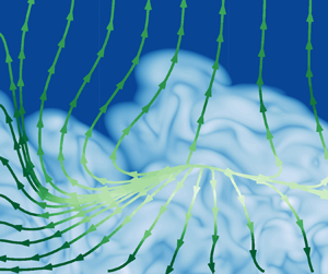
The flow problem considered here is for a Reynolds number $Re = U_0 H / \nu = 1000$; see figure 1 for a view of the enstrophy field. The computational domain is a cuboid of size $96H \times 96H \times 48H$ and has been discretized by using $2304 \times 2304 \times 960$ elements. A variable time step has been used for the temporal integration in order to obtain a condition $CFL < 0.3$. Three simulations have been performed. Every simulation is started from the same initial conditions (2.2) except for the perturbation superimposed. Hence, these simulations allow us to have statistically independent flow realizations and have been used to improve the statistical convergence of the data by using the ensemble average. From the initial conditions, the flow field is let to freely evolve in time. The total integration time for each simulation is $t = 160$. When not specifically stated, in what follows variables are presented dimensionless by using $H$ for lengths and $H/U_0$ for times.

Figure 1. Direct numerical simulation of a planar temporal jet. Instantaneous flow realization at $t =120$ shown by means of iso-contours of the enstrophy field. Contour colours follow an exponential distribution. The flow domain shown is truncated in $z$ for readability reasons.

After an initial transition when the system develops turbulence, the flow decays and approaches a self-similar regime (Redford, Castro & Coleman Reference Redford, Castro and Coleman2012; Djenidi et al. Reference Djenidi, Antonia, Lefeuvre and Lemay2016) characterized by a constant Taylor Reynolds number, $Re_\lambda = \sqrt {2k_{cl}/3} \lambda _{cl} / \nu = 50$, where $k_{cl}$ is the centreline turbulent kinetic energy and $\lambda = \sqrt {10 \nu k_{cl} / \epsilon _{cl}}$ is the Taylor microscale with $\epsilon _{cl}$ the centreline turbulent dissipation. By following van Reeuwijk & Holzner (Reference van Reeuwijk and Holzner2014), the self-similar regime can be further characterized by a temporal scaling of the characteristic velocities which is proportional to $t^{-1/2}$ and of the characteristic lengths which is proportional to $t^{1/2}$. Figure 2 confirms these behaviours. In particular, it appears that turbulence has reached a dynamic equilibrium for $t>60$ when all the observables start to follow a self-similar behaviour. Figure 2 also shows the quality of the grid resolution adopted to perform the simulations. Indeed, the minimum value of the centreline Kolmogorov scale $\eta = (\nu ^{3} / \epsilon _{cl})^{1/4}$ is shown to be reached for $t=40$, leading to a grid resolution ${\rm \Delta} x_{1,2} / \eta \approx 1.66$ and ${\rm \Delta} x_{3} / \eta \approx 2$. The resolution employed is even more appropriate if we consider that the Kolmogorov scale increases from this minimum with time as $\eta \sim \sqrt {t}$ and with the cross-flow position $z$ since dissipation is maximum at the centreline.

Figure 2. Temporal behaviours of relevant statistical observables. (a) Centreline mean velocity $U_{cl}(t)$. The inset shows the centreline turbulent kinetic energy $k_{cl}(t)$ and turbulent dissipation $\epsilon _{cl}(t)$. (b) Jet half-widths computed as the 50 % of the mean centreline velocity, $h_{1/2}(t)$, and as the 2 % of the mean centreline velocity and enstrophy values, $h_{U}(t)$ and $h_{\varOmega }(t)$, respectively. The inset show the Kolomogorov $\eta$ and Taylor $\lambda$ scales evaluated at the centreline.

The computational domain is four times and twelve times larger in the two homogeneous directions with respect to the domain used in van Reeuwijk & Holzner (Reference van Reeuwijk and Holzner2014) and da Silva & Pereira (Reference da Silva and Pereira2008), respectively. This very large domain has been used in order to accurately resolve the largest scales of the flow, thereby allowing us to improve the statistical convergence because of the larger area spanned by the two homogeneous directions. Indeed, the extent of the flow domain used in the present work is a result of the study of the velocity two-point correlations from different simulations with different domain sizes. In particular, two additional simulations with the same numerical setting but different domain lengths, $24H \times 24H \times 36H$ and $72H \times 48H \times 36H$, have also been considered. As shown in figure 3, the correlation coefficient of streamwise velocity,

(2.3)\begin{equation} C_{uu} (r_i,z,t) = \frac{\langle u'(x_i+r_i,z,t) u'(x_i,z,t)\rangle}{\langle u'u'\rangle (z,t)} , \end{equation}

highlights significant differences in terms of correlation and anti-correlation lengths and shapes by varying the domain size. In particular, only the largest domain size appears to show a clear decorrelation of the velocity field. These results clearly highlight the need of using very large domains in order to capture the statistically relevant largest scales of the flow. It is worth pointing out that in such a flow configuration, the largest scales are represented by the large-scale vortices originating from the Kelvin–Helmholtz instability. Given the inviscid nature of this instability, we argue that such a constraint on the domain size is not mitigated by an increase of the Reynolds number.

Figure 3. Two-point correlation coefficient of streamwise velocity, $C_{uu}$, evaluated at the centreline for $t=120$ as a function of the streamwise increment $r_x$ (a) and of the spanwise one $r_y$ (b). Results from three simulations with a different domain size: $24H \times 24H \times 36H$ (dashed–dotted line), $72H \times 48H \times 36H$ (dashed line) and $96H \times 96H \times 48H$ (solid line).

In the present work, average quantities denoted as $\langle \cdot \rangle$ are computed by making use of the ensemble average between the different flow realizations and by taking advantage of the statistical symmetries of the flow. In particular, a spatial average is also performed in the two statistically homogeneous streamwise and spanwise directions. Furthermore, the flow exhibits a statistical symmetry in the cross-flow direction so that a transformation $z \rightarrow -z$ leaves quantities such as $\langle u \rangle$ and $\langle u_i u_i \rangle$ statistically invariant while reversing the sign of quantities such as $\langle u w \rangle$ and $\partial \langle \cdot \rangle / \partial z$. In conclusion, the average of a generic quantity $\beta$ is defined as

(2.4)\begin{align} \langle \beta \rangle (z, t) = \frac{1}{N} \sum_{i=1}^{N} \frac{1}{2}\left (\frac{1}{L_x L_y} \iint \beta (x,y,z,t)\, {\textrm{d}{\kern0.08em} x} {\textrm{d} y} \pm \frac{1}{L_x L_y} \iint \beta (x,y,-z,t)\, {\textrm{d}{\kern0.08em} x} {\textrm{d}y} \right)\!, \end{align}

where $N=3$ is the number of flow realizations simulated and $L_x$ and $L_y$ are the dimensions of the flow domain in the streamwise and spanwise directions. In the following, the Kolmogorov length and velocity scales, $\eta$ and $u_\eta$, will be used for the non-dimensionalization of flow variables and will be denoted with a superscript $*$; see appendix A for the related scaling in the self-similar regime. Finally, the customary Reynolds decomposition of the flow in a mean and fluctuating field will be adopted, i.e. $u_i = U_i + u_i^{\prime }$.

3. Theoretical framework

Temporal jets are freely evolving turbulent flows characterized by a flux of momentum and kinetic energy both in space and time. In the case of planar jets, these transports in physical space occur on average only in the cross-flow direction. In these flow settings, the mean momentum equations read as

(3.1)\begin{gather} \frac{\partial U}{\partial t} +\frac{\partial}{\partial z} \underbrace{\left ( \langle u' w' \rangle - \nu \frac{\partial U}{\partial z} \right )}_{\varphi_{13} = \varphi_{13}^{turb} + \varphi_{13}^{visc}} = 0, \end{gather}

(3.2)\begin{gather}\frac{\partial}{\partial z} \underbrace{\left ( \frac{P}{\rho} + \langle w' w' \rangle \right )}_{\varphi_{33} = \varphi_{33}^{press} + \varphi_{33}^{turb}} = 0 . \end{gather}

The only non-zero mean momentum is in the streamwise direction, $U$, and its flux in time is given by the unbalance of its turbulent and viscous fluxes in the cross-flow direction, $\varphi _{13} = \varphi _{13}^{turb} + \varphi _{13}^{visc}\! \neq 0$. On the contrary, the mean momentum in the cross-flow direction is null and turbulent and pressure fluxes in the cross-flow direction balance themselves, $\varphi _{33} = \varphi _{33}^{press} + \varphi _{33}^{turb}=0$. As already stated, also the mean and turbulent kinetic energy is characterized by a flux in time and in the cross-flow direction. The mean kinetic energy budget reads as

(3.3)\begin{equation} \frac{\partial K}{\partial t}={-} \frac{\partial}{\partial z} \underbrace{\left ( \langle u' w' \rangle U - \nu \frac{\partial K}{\partial z} \right )}_{\varPsi_z = \varPsi_z^{turb} + \varPsi_z^{visc}} \underbrace{+ \langle u' w' \rangle \frac{\partial U}{\partial z}}_{{-}P_t} - \underbrace{\nu \frac{\partial U}{\partial z} \frac{\partial U}{\partial z}}_{E} , \end{equation}

where $K=UU/2$, while the turbulent kinetic energy budget is

(3.4)\begin{equation} \frac{\partial \langle k \rangle}{\partial t}={-} \frac{\partial}{\partial z} \underbrace{\left ( \langle k w' \rangle + \frac{1}{\rho}\langle p' w' \rangle - \nu \frac{\partial \langle k \rangle}{\partial z} \right )}_{\psi_z = \psi_z^{turb} + \psi_z^{press} + \psi_z^{visc}} \underbrace{- \langle u' w' \rangle \frac{\partial U}{\partial z}}_{P_t} - \underbrace{\nu \left\langle \frac{\partial u_i'}{\partial x_j} \frac{\partial u_i'}{\partial x_j} \right\rangle}_{\epsilon} ,\end{equation}

where $k=u_i' u_i' / 2$. Contrary to the mean momentum balance equations, source and sink terms also appear together with spatial fluxes in the cross-flow direction in the kinetic energy budget equations. In particular, in the mean kinetic energy budget (3.3), only a sink term appears that is the sum of production of turbulent fluctuations, $P_t$, and viscous dissipation by mean shear, $E$. The unbalance of this sink with the transport due to turbulent and viscous fluxes, $\partial \varPsi _z / \partial z$, governs the time variation of mean kinetic energy. In the turbulent kinetic energy budget (3.4), the turbulence production term $P_t$ is, on the contrary, a source. Hence, the sum $P_t-\epsilon$ can be both positive and negative, thus establishing source and sink flow regions. The energy transports due to turbulent, pressure and viscous fluxes, $\partial \psi _z / \partial z$, partially conform with these regions by extracting energy in the source and releasing it in the sink regions. The unbalance between source/sink and spatial transports governs the flux of turbulent kinetic energy in time.

The class of processes described by the mean momentum and energy budget equations are phenomena that occur in physical space. Hence, in the context of free-shear flows, these equations enable the study of the phenomena and positions where momentum and turbulence are developed and the transport mechanisms sustaining the spreading and entrainment of the jet. However, turbulence is known to also be characterized by phenomena taking place in the space of scales such as the turbulent cascade and, in free-shear flows, the large-scale engulfment and small-scale nibbling mechanisms of entrainment. This duality of description of the same physical phenomenon is a result of the statistical observables used for its study. The drawback is the development of different theories as spurious results of approaches that do not support the occurrence of phenomena simultaneously involving different scales and positions.

To overcome this scale/position duality, in the present work we propose the use of an alternative formalism, the so-called generalized Kolmogorov equation (Hill Reference Hill2002). It is a differential equation that, in its original form valid for homogeneous and isotropic turbulence, can be traced back to Kolmogorov himself (Kolmogorov Reference Kolmogorov1991a,Reference Kolmogorovb). The theoretical framework is based on the exact equation for the second-order moment of the velocity increment, $\delta u_i = u_i' (\boldsymbol {x''}, t) - u_i' (\boldsymbol {x'}, t)$, the so-called second-order structure function, $\delta q^{2} = \delta u_i \delta u_i$ (Dubrulle Reference Dubrulle2019). The second-order structure function depends both on the separation vector $r_i = x_i''-x_i'$ and on the position of the mid-point $x_{ci} = (x_i''+x_i')/2$. Hence, in the general case $\langle \delta q^{2} \rangle$ depends upon seven independent variables, the three coordinates of the mid-point position $\boldsymbol {x}_{\boldsymbol {c}}$, the three-dimensional scale separation $\boldsymbol {r}$ and time $t$. The generalized Kolmogorov equation has been used in several works to study the energetics of turbulence in the complete space of scales and positions, we mention only few of them, e.g. Danaila et al. (Reference Danaila, Anselmet, Zhou and Antonia2001), Marati, Casciola & Piva (Reference Marati, Casciola and Piva2004), Cimarelli et al. (Reference Cimarelli, De Angelis and Casciola2013, Reference Cimarelli, De Angelis, Schlatter, Brethouwer, Talamelli and Casciola2015b, Reference Cimarelli, De Angelis, Jimenez and Casciola2016), Saikrishnan et al. (Reference Saikrishnan, De Angelis, Longmire, Marusic, Casciola and Piva2012) for turbulent channel flows, Mollicone et al. (Reference Mollicone, Battista, Gualtieri and Casciola2018) for separated flows, Rincon (Reference Rincon2006), Togni, Cimarelli & De Angelis (Reference Togni, Cimarelli and De Angelis2015, Reference Togni, Cimarelli and De Angelis2019) for thermally driven turbulence, Gomes-Fernandes, Ganapathisubramani & Vassilicos (Reference Gomes-Fernandes, Ganapathisubramani and Vassilicos2015); Portela, Papadakis & Vassilicos (Reference Portela, Papadakis and Vassilicos2017) for turbulent wakes and Burattini, Antonia & Danaila (Reference Burattini, Antonia and Danaila2005), Sadeghi, Lavoie & Pollard (Reference Sadeghi, Lavoie and Pollard2016) for round jets. Here, we extend the use of the generalized Kolmogorov equation to the symmetries of a turbulent planar temporal jet. The equation reads as

(3.5)\begin{align} &\frac{\partial \langle \delta q^{2} \rangle}{\partial t} + \underbrace{\frac{\partial \langle \delta q^{2} \delta u_i^{\prime} \rangle }{\partial r_i} + \frac{\partial \langle \delta q^{2} \delta U \rangle }{\partial r_x}}_{{-}T_r} - \underbrace{ 2 \nu \frac{\partial^{2} \langle \delta q^{2} \rangle }{\partial r_i \partial r_i}}_{{-}D_r} + \underbrace{\frac{\partial \langle \delta q^{2} \tilde{w}^{\prime} \rangle }{\partial z_c} + \frac{2}{\rho}\frac{\partial \langle \delta p^{\prime} \delta w^{\prime} \rangle}{\partial z_c} - \frac{\nu}{2} \frac{\partial^{2} \langle \delta q^{2} \rangle}{\partial z_c \partial z_c}}_{{-}T_z} \nonumber\\ &\quad =\underbrace{- 2 \langle \delta u^{\prime} \delta w^{\prime} \rangle \widetilde{ \left ( \frac{\partial U}{\partial z} \right )} - 2 \langle \delta u^{\prime} \tilde{w}^{\prime} \rangle \delta \left ( \frac{\partial U}{\partial z} \right )}_{\varPi} - 4 \underbrace{\nu \widetilde{\left\langle \frac{\partial u_i'}{\partial x_j} \frac{\partial u_i'}{\partial x_j} \right\rangle}}_{\tilde{\epsilon}}, \end{align}

where $\widetilde {\cdot }$ denotes the two-point mean operator that, for a generic quantity, reads as $\tilde {\beta } = (\beta (\boldsymbol {x''}, t) + \beta (\boldsymbol { x'}, t))/2$. To highlight its conservative form, (3.5) can be rewritten as

(3.6)\begin{equation} \frac{\partial \langle \delta q^{2} \rangle}{\partial t} + \frac{\partial \phi_{r_i}}{\partial r_i} + \frac{\partial \phi_{z_c}}{\partial z_c}= \xi, \end{equation}

where

(3.7)\begin{gather} \frac{\partial \phi_{r_i}}{\partial r_i} = \frac{\partial}{\partial r_i} (\phi_{r_i}^{turb} + \phi_{r_i}^{mean} + \phi_{r_i}^{visc} ), \end{gather}

(3.8)\begin{gather}\frac{\partial \phi_{z_c}}{\partial z_c} = \frac{\partial}{\partial z_c} (\phi_{z_c}^{turb} + \phi_{z_c}^{press} + \phi_{z_c}^{visc}) \end{gather}

are the divergence of fluxes occurring in the space of scales $r_i$ and in physical space $z_c$, respectively. In particular, the scale-space flux $\phi _{r_i}$ is given by three contributions

(3.9a–c)\begin{equation} \phi_{r_i}^{turb} = \langle \delta q^{2} \delta u_i^{\prime} \rangle, \quad \phi_{r_i}^{mean} = \langle \delta q^{2} \delta U \rangle \delta_{i1}, \quad \phi_{r_i}^{visc} ={-} 2 \nu \frac{\partial \langle \delta q^{2} \rangle}{\partial r_i} \end{equation}

due to inertial turbulent fluctuations, to mean advection and to viscous diffusion, respectively. On the other hand, the spatial flux is given by three contributions

(3.10a–c)\begin{equation} \phi_{z_c}^{turb} = \langle \delta q^{2} \tilde{w}^{\prime} \rangle, \quad \phi_{z_c}^{press} = \frac{2}{\rho} \langle \delta p^{\prime} \delta w^{\prime} \rangle, \quad \phi_{z_c}^{visc} ={-} \frac{\nu}{2} \frac{\partial \langle \delta q^{2} \rangle}{\partial z_c} \end{equation}

due to inertial turbulent fluctuations, to pressure fluctuations and viscous diffusion, respectively. These transport terms are partially driven by a source term which is the balance between turbulence production and dissipation,

(3.11)\begin{equation} \xi = \varPi - 4 \tilde{\epsilon} . \end{equation}

The unbalance between transports and sources governs the flux of scale energy in time, that in a symbolic form reads as

(3.12)\begin{equation} \frac{\partial \langle \delta q^{2} \rangle}{\partial t} = T_r + D_r + T_z + \xi . \end{equation}

In line with the single-point energy budgets, the generalized Kolmogorov equation allows for the study of the source and sink regions of the flow and of the fluxes connecting these regions. However, the strength of the formalism is such that all these processes are both scale and position dependent, and, as a consequence, also fluxes in the space of scales can be defined, i.e. $\phi _{r_i}$.

4. Inhomogeneity and flow regions

Before analysing the compound space of scales and positions described by the generalized Kolmogorov equation (3.5), it is useful to divide the flow in different regions characterized by well-defined physical processes. Indeed, the flow while freely evolving in time, is characterized by a strong statistical inhomogeneity in the cross-flow direction as clearly highlighted by the mean velocity and turbulent intensity profiles shown in figure 4(a). In particular, the flow can be idealized as characterized by a turbulent core where the mean flow and the turbulent fluctuations are intense and by an interface region where entrainment processes occur. From the mean flow point of view, both these two flow regions are characterized by a cross-flow spreading. As shown in figure 4(b), a positive turbulent flux of mean streamwise momentum in the cross-flow direction, $\varphi _{13}^{turb} > 0$, is found to cover the entire flow domain. The intensity of the turbulent flux far exceeds the still positive contribution given by the viscous flux, $\varphi _{13}^{visc} \approx 0$, thus sustaining a spreading of the mean streamwise momentum profile $\varphi _{13} = \varphi _{13}^{turb}+\varphi _{13}^{visc} > 0$. As a consequence, the time variation of the mean streamwise momentum is positive in the outer jet region $\partial U / \partial t > 0$ and negative in the inner jet region $\partial U / \partial t < 0$. The cross-over between decaying and enhancing mean momentum is $z^{*} \approx 60$, corresponding to the peak value of the turbulent flux $\varphi _{13}^{turb}$. Due to the symmetries of the flow, the mean cross-flow momentum is zero and, as shown in the inset of figure 4(b), a balance of positive turbulent flux, $\varphi _{33}^{turb} > 0$, and negative pressure flux, $\varphi _{33}^{press} < 0$, takes place.

Figure 4. (a) Mean velocity and turbulent intensity profiles: $U^{*}$ (solid line), $\sqrt {\langle u'u' \rangle ^{*}}$ (dashed line), $\sqrt {\langle v'v' \rangle ^{*}}$ (dashed–dotted line) and $\sqrt {\langle w'w' \rangle ^{*}}$ (dotted line). (b) Mean momentum equation. Main panel: $10 \partial U^{*}/\partial t^{*}$ (delta), mean streamwise momentum fluxes $\varphi _{13}^{turb *}$ (solid) and $\varphi _{13}^{visc *}$ (dash). Inset panel: mean cross-flow momentum fluxes $\varphi _{33}^{turb *}$ (solid) and $\varphi _{33}^{press *}$ (dash).

In line with the processes governing momentum, the mean kinetic energy budget also highlights that the entire flow domain is characterized by a cross-flow spreading. As shown in the inset of figure 5, the temporal jet is characterized by a continuous flux of mean kinetic energy from its core towards the outer interface region, $\varPsi _z = \varPsi _z^{turb}+ \varPsi _z^{visc} > 0$. Both viscous diffusion and turbulent fluxes are positive but the contribution of the turbulent flux far exceeds that due to viscosity, $\varPsi _z^{turb} \gg \varPsi _z^{visc} >0$. As a consequence, the turbulent transport term $\partial \varPsi _z^{turb} / \partial z$ is the dominant term of the budget. As shown in the main panel of figure 5, $\partial \varPsi _z^{turb} / \partial z$ drains kinetic energy for $z^{*} < 45$ to feed the outer region of the jet for $z^{*} > 45$ with a peak intensity at $z^{*} \approx 80$. The other terms of the budget are negligible with the exception of the turbulence production term $-P_t$ which drains kinetic energy from the mean flow to sustain turbulent fluctuations and, hence, it is negative with a peak intensity at $z^{*} \approx 60$. These two processes of turbulence production and turbulent transport govern the behaviour of mean kinetic energy and their unbalance results in a time variation of mean kinetic energy. In accordance with the mean momentum results, the cross-over between decaying and enhancing mean kinetic energy is $z^{*} \approx 60$.

Figure 5. Mean kinetic energy budget. Main panel: $\partial K^{*} / \partial t^{*}$ (delta), $-P_t^{*}$ (solid), $-E^{*}$ (dash), $-\partial \varPsi _z^{turb *} / \partial z^{*}$ (dash-dot) and $-\partial \varPsi _z^{visc *} / \partial z ^{*}$ (dash–dot–dot). Insets: $\varPsi _z^{turb *}$ (dash–dot) and $\varPsi _z^{visc *}$ (dash–dot–dot).

Contrary to the mean momentum and mean kinetic energy processes, the behaviour of turbulent kinetic energy allows us to characterize the flow in different flow regions depending on the physical process sustaining turbulence. As shown in figure 6(a), turbulence production $P_t$ is active in an intermediate region in between the core and outer part of the jet where the mean shear is maximum; see also figure 4(a). On the other hand, turbulent dissipation $-\epsilon$ shows a decrease of its intensity moving from the jet core towards the interface region. The spatial transport $-\partial \psi _z / \partial z$ is dominated by the turbulent and pressure terms being that the viscous diffusion is negligible almost everywhere, $\partial \psi _z / \partial z \approx \partial (\psi _z^{turb} + \psi _z^{press}) / \partial z$.

Figure 6. Turbulent kinetic energy budget. Main panels: $\partial \langle k \rangle ^{*}/\partial t^{*}$ (delta), $P_t^{*}$ (solid), $-\epsilon ^{*}$ (dash), $-\partial \psi _z^{turb *} / \partial z^{*}$ (dash–dot), $-\partial \psi _z^{press *} / \partial z^{*}$ (dot) and $-\partial \psi _z^{visc *} / \partial z^{*}$ (dash–dot–dot). Insets: $\psi _z^{turb *}$ (dash–dot), $\psi _z^{press *}$ (dot) and $\psi _z^{visc *}$ (dash–dot–dot). The overall behaviour is shown in (a) while an enlargment of the behaviour in the interface region is shown in (b).

The overall picture is the following. In the intermediate region, $15 < z^{*} < 106$ (production region I), fluctuations are mainly sustained by turbulence production. The available turbulent energy is drained by both local turbulent dissipation processes $-\epsilon$ and by turbulent transport mechanisms $-\partial \psi _z^{turb} / \partial z < 0$ which overcomes the opposite in sign pressure transport contribution $-\partial \psi _z^{turb} / \partial z>0$. The balance is negative giving rise to a peak of turbulent kinetic energy decay in time within this region, $\partial \langle k \rangle /\partial t < 0$. The energy subtracted by the turbulent transport is then transferred towards the inner and outer regions of the jet. In particular, for $z^{*} < 15$ (inner region II) and $z^{*} > 106$ (outer region III), the dominant process sustaining turbulence is the turbulent transport, $-\partial \psi _z^{turb} / \partial z > 0$, and the budget in these two regions reduces to

(4.1)\begin{equation} \frac{\partial \langle k \rangle}{\partial t} \approx{-} \frac{\partial}{\partial z} (\psi_z^{turb} + \psi_z^{press}) -\epsilon \end{equation}

since production is almost negligible. The main difference between these two regions is that in the inner region II both turbulent and pressure transports are positive, $-\partial \psi _z^{turb} / \partial z > -\partial \psi _z^{press} / \partial z > 0$, but the balance with dissipation is negative leading to a turbulent energy decay, $\partial \langle k \rangle /\partial t < 0$. On the contrary, in the outer region III the pressure transport is negative but the turbulent transport is positive and large enough to have a positive balance with dissipation leading to $\partial \langle k \rangle /\partial t > 0$ and reaching its maximum for $z^{*} \approx 125$.

Overall, we observe that, for $z^{*} < 180$, the turbulent transport is more intense than the pressure one and plays a role of draining of turbulent energy from region I to feed regions II and III. Accordingly, as shown in the inset of figure 6(a), a cross-over location $z^{*} \approx 40$ can be defined splitting the flow in regions traversed by a negative turbulent flux, $\psi _z^{turb} < 0$, directed towards the jet centreline for $z^{*} < 40$ from regions traversed by a positive flux, $\psi _z^{turb} > 0$, towards the jet interface for $z^{*} > 40$. On the other hand, pressure transport drains turbulent energy in the outer region III to feed the inner regions of the jet (regions I and II). Hence, for $z^{*} < 180$, the turbulent jet is entirely traversed by a negative pressure flux, $\psi _z^{press} < 0$, as shown in the inset of figure 6(a). Note that the jet interface defined as the 2 % of the jet centreline enstrophy is located at $z^{*} = h_{\varOmega }^{*} = 171$.

Different considerations can be drawn for the external region IV, for $z^{*} > 180$, i.e. further away from the putative jet interface at $z^{*} = h_{\varOmega }^{*} = 171$. As for the outer region III, fluctuations in this region of the flow are sustained by transport mechanisms. However, as shown in figure 6(b), in this case the contribution of the pressure transport turns out to be positive, $-\partial \psi _z^{press} / \partial z > 0$ and, for $z^{*} > 210$, it overcomes the contribution of the turbulent transport, i.e. $-\partial \psi _z^{press} / \partial z > -\partial \psi _z^{turb} / \partial z > 0$. Interestingly, for $z^{*} > 210$, the turbulent dissipation is almost null, thus suggesting that the fluctuations observed at the external region of the jet are not turbulent in nature. Hence, in this region the balance reduces to

(4.2)\begin{equation} \frac{\partial \langle k \rangle}{\partial t} \approx{-} \frac{\partial \psi_z^{press}}{\partial z} > 0 . \end{equation}

We conjecture that such time increasing of the kinetic energy content is induced by large-scale pressure fluctuations induced by the large-scale vortex pattern of the jet reminiscent of the Kelvin–Helmholtz instability. Hence, we argue that the transport of turbulent kinetic energy also occurs in the non-turbulent region further away from the jet interface throughout non-local interactions of the large-scale jet pattern with the surrounding quiescent fluid mediated by the pressure field, $\partial \psi _z^{press}/\partial z$. These aspects will be further investigated in § 6.5 by means of a scale-by-scale analysis.

5. Scale-energy paths

We now extend the analysis of the turbulent temporal planar jet to the augmented space of turbulence $(r_x, r_y, r_z, z_c, t)$ described by the generalized Kolmogorov equation (3.5). The multi-dimensionality of the approach challenges for a rational study. For this reason, we will limit the analysis to the hyper-planes $(r_z=0, t={\rm const})$ and $(r_x=0, t= {\rm const})$ of the five-dimensional space of locations, scales and times. The resulting equations retain their conservative form,

(5.1)\begin{gather} \frac{\partial \phi_{r_x} (r_x,r_y,z_c)}{\partial r_x} + \frac{\partial \phi_{r_y} (r_x,r_y,z_c)}{\partial r_y} + \frac{\partial \phi_{z_c} (r_x,r_y,z_c)}{\partial z_c}= \zeta_{r_z=0} \quad (r_z=0, t= \textrm{const}), \end{gather}

(5.2)\begin{gather}\frac{\partial \phi_{r_y} (r_y,r_z,z_c)}{\partial r_y} + \frac{\partial \phi_{r_z} (r_y,r_z,z_c)}{\partial r_z} + \frac{\partial \phi_{z_c} (r_y,r_z,z_c)}{\partial z_c}= \zeta_{r_x=0} \quad (r_x=0, t= \textrm{const}), \end{gather}

thus showing that scale-energy fluxes in the hyper-planes are driven by extended source terms,

(5.3)\begin{gather} \zeta_{r_z=0} = \xi - \frac{\partial \phi_{r_z}}{\partial r_z} - \frac{\partial \langle \delta q^{2} \rangle}{\partial t}, \end{gather}

(5.4)\begin{gather}\zeta_{r_x=0} = \xi - \frac{\partial \phi_{r_x}}{\partial r_x} - \frac{\partial \langle \delta q^{2} \rangle}{\partial t}, \end{gather}

which take into account the scale energy exchange with the local sink/source phenomena, $\xi$, and with the dimensions perpendicular to the hyper-plane considered, i.e.

(5.5)\begin{gather} - \frac{\partial \phi_{r_z}}{\partial r_z} - \frac{\partial \langle \delta q^{2} \rangle}{\partial t} \quad \mbox{for} \quad (r_z=0, t= \textrm{const}), \end{gather}

(5.6)\begin{gather}- \frac{\partial \phi_{r_x}}{\partial r_x} - \frac{\partial \langle \delta q^{2} \rangle}{\partial t} \quad \mbox{for} \quad (r_x=0, t= \textrm{const}) . \end{gather}

Hence, the divergence of fluxes in the hyper-planes can be understood as the intensity of scale energy extracted/released by the flux vector field along its trajectories. In equilibrium turbulence the divergence of fluxes in the hyper-planes always balances with the sum of the local source term $\xi$ (production minus dissipation) and with the scale energy exchange to/from the scale space perpendicular to the hyper-plane itself, $\partial \phi _{r_\perp }/\partial r_\perp$, thus, $\partial \langle \delta q^{2} \rangle / \partial t = 0$. In non-equilibrium turbulence such as in the temporal jet, the divergence of fluxes in the hyper-plane can exceed/subceed the sum $\xi - \partial \phi _{r_\perp }/\partial r_\perp$, thus enabling a scale-energy transfer in time $\partial \langle \delta q^{2} \rangle / \partial t \neq 0$.

5.1. The hyper-plane $(r_z=0, t=120)$

We start the analysis by considering the hyper-plane $(r_z=0, t=120)$. In figure 7 the trajectories of the flux vector field, $(\phi _{r_x},\phi _{r_y},\phi _{z_c})$, coloured by the intensity of scale energy extracted/released along their route, $\partial \phi _{r_x}/\partial r_x + \partial \phi _{r_y}/\partial r_y + \partial \phi _{z_c}/\partial z_c$, are shown. The plots show that all the fluxes emerge from a well-defined point of the augmented space, $(r_x^{*}, r_y^{*}, z_c^{*}) \approx (90, 110, 60)$. As shown in figure 7(a) with an iso-surface of $\langle \delta q^{2} \rangle = 0.98 \langle \delta q^{2} \rangle _{max}$, this singularity point belongs to a range of scales and positions of the augmented space characterized by the largest scale-energy content. This energy-containing region takes a toroid shape that in physical space lies in the $z_c^{*} \approx 60$ plane. A well-defined band of energy-containing scales is also identified by the iso-surface of $\langle \delta q^{2} \rangle = 0.98 \langle \delta q^{2} \rangle _{max}$ that can be traced by considering the radius of revolution of this toroid shape. We find that the radius is not constant and equals $r_y^{*} \approx 160$ for $r_x^{*}=0$ and $r_x^{*} \approx 140$ for $r_y^{*}=0$, thus highlighting the anisotropy of the large energy-containing scales of the flow. As it can be grasped from the iso-contours of figures 7(b) and 7(c), this range of scales and positions is also the site of the local turbulence production mechanisms being that the source term is maximum and positive, $\xi > 0$, i.e. turbulence production exceeds dissipation in this region of the augmented space. By considering that the jet half-width is $h_{\varOmega }^{*} = 171$ (evaluated as the location where enstrophy is 2 % of the jet centreline enstrophy), we can assert that this toroidal source region of energy-containing fluctuations occurs at length scales of the same order of the integral scale of the problem.

Figure 7. Paths of scale energy in the hyper-plane $r_z = 0$. Trajectories of the flux vector field, $(\phi _{r_x},\phi _{r_x},\phi _{z_c})$, coloured by the intensity of scale energy extracted/released along their route, $\partial \phi _{r_x}/\partial r_x + \partial \phi _{r_y}/\partial r_y + \partial \phi _{z_c}/\partial z_c$. The iso-surface in panel (a) reports the energy-containing region of the augmented space of scales and positions, $\langle \delta q^{2} \rangle = 0.98 \langle \delta q^{2} \rangle _{max}$. In panels (b) and (c) two lateral views are reported together with the iso-contours of the source term $\xi$ evaluated in the planes $r_y=0$ and $r_x=0$, respectively.

In accordance with the above analysis, we can assert that the field of fluxes stems from the source and energy-containing region of the augmented space of scales and positions. A more detailed analysis shows that from the singularity point $(r_x^{*}, r_y^{*}, z_c^{*}) \approx (90, 110, 60)$, the fluxes bifurcate in three distinct branches approaching the $z_c$-distributed small-scale range, the inner region of the jet and outer regions of the jet; see figure 7(a). These three regions are the sink regions of the augmented space of turbulence where scale energy is eventually conveyed. Note the complex nature of the scale-energy paths towards these three regions which deserves the following separate analysis.

5.1.1. Family of fluxes $\mathcal {A}$

The first family of fluxes is that feeding the $z_c$-distributed dissipative range of small scales. This branch of fluxes while diverging from the singularity point systematically move towards smaller streamwise and spanwise scales, $\phi _{r_x} < 0$ and $\phi _{r_y} < 0$, respectively. As better shown in figures 7(b) and 7(c), after an initial ascension towards outer positions, $\phi _{z_c} > 0$, this family of fluxes bends, attaining a flow towards inner positions, $\phi _{z_c} < 0$. This picture is maintained for the entire range of inertial and energy-containing scales, $r^{*} >\textit{O}(20)$, where $r^{*} \equiv (r_x^{*2} + r_y^{*2})^{1/2}$. In fact, an interesting aspect appears in the final range of scales intercepted by the fluxes. As clearly shown in figure 7, by entering the dissipative range of small scales, $r^{*} < \textit{O}(20)$, the fluxes show a second reversal of the spatial flux towards outer positions, $\phi _{z_c} > 0$. As a consequence, the entire $z_c$-distributed range of small scales is found to be intercepted by the branch of fluxes $\mathcal {A}$. The effect of spatial inhomogeneity vanishes only at very small separations where, the small-scale asymptotic is $(\phi _{r_x},\phi _{r_y},\phi _{z_c}) \sim (1,1,0)r^{*}$ (Cimarelli et al. Reference Cimarelli, De Angelis and Casciola2013) and, hence, the fluxes become asymptotically orthogonal to the $z_c$-axis.

As shown by the intensity of the flux divergence reported with colours in figure 7, the field of fluxes extracts scale energy from the large energy-containing scales of the turbulence production region I and releases it to the $z_c$-distributed dissipative range of small scales. The overall picture is that of a $z_c$-distributed dissipative range of small scales fed by an ascending direct energy cascade whose origin can be traced back to the inertial scales of the inner region and, before that, to the energy-containing scales of the production region. Hence, the behaviour of the family of fluxes $\mathcal {A}$ is entirely consistent with the picture of a Richardson turbulent energy cascade superimposed to inhomogeneous spatial redistribution processes.

We investigate here more in detail the origin of the observed inversion of the spatial flux along the paths of the family of fluxes $\mathcal {A}$. In particular, we observed that, in the inertial and energy-containing scales $r^{*} > \textit{O}(20)$, the spatial flux is negative and directed towards the inner region of the jet while, in the dissipative scales $r^{*} < \textit{O}(20)$, the spatial flux becomes positive thus reversing towards the outer regions of the jet. The reason of the small-scale ascending phenomenon is given by the concurrent role played by the turbulent and pressure spatial fluxes. In figure 8 the behaviours of the total spatial flux $\phi _{z_c}$, the turbulent spatial flux $\phi _{z_c}^{turb}$ and the pressure spatial flux $\phi _{z_c}^{press}$ are shown in the $(r_y,r_z) = (0,0)$ plane. In accordance with the single-point budgets shown in § 4, the pressure flux is negative, $\phi _{z_c}^{press} < 0$, for the entire jet width, $z_c^{*} < 170$, and positive, $\phi _{z_c}^{press} > 0$, only in the external transitional region of the jet, $z_c^{*} > 170$; see the dashed line in figure 8(c). The maximum of the inward pressure flux is reached at the energy-containing scales, $r^{*} = \textit{O}(130)$. On the other hand, the turbulent spatial flux spreads from the production region, thus showing an inward flux $\phi _{z_c}^{turb} < 0$ for $z_c^{*} < 40$ and an outward flux $\phi _{z_c}^{turb} > 0$ for $z_c^{*} > 40$; see figure 8(b). The spatial turbulent flux is active for a wide range of scales encompassing both inertial and energy-containing scales, contrary to the pressure flux where a peak activity is measured for the energy-containing scales $r^{*} = \textit{O}(130)$. Hence, (i) the turbulent flux is more active than the pressure flux at inertial and dissipative scales. Furthermore, (ii) the turbulent flux is found to be positive at small dissipative scales, $r^{*} < \textit{O}(20)$, for the entire jet width, also in the inner region where, for larger scales, is directed towards the jet centreline; see the dashed line in figure 8(b). The combined effect of these two aspect leads to a total spatial flux $\phi _{z_c} \approx \phi _{z_c}^{turb} + \phi _{z_c}^{press}$ being $\phi _{z_c}^{visc} \approx 0$ almost everywhere, with three peak activities; see figure 8(a). Two peaks of outward flux centred at $z_c^{*} =100$ involving separately small $r^{*} = \textit{O}(30)$ and very large scales $r^{*} = \textit{O}(280)$. One peak activity of inward flux centred at $z_c^{*} =30$ sustaining the large scales $r^{*} = \textit{O}(200)$ of the inner region of the jet. On the other hand, the small dissipative scales of the entire jet width $r^{*} < \textit{O}(20)$ are involved in an outward flux, thus explaining the observed ascending direct energy cascade feeding the $z_c$-distributed dissipative range of small scales in figure 7.

Figure 8. Iso-contours of (a) the total spatial flux $\phi _{z_c}$, (b) the spatial turbulent flux $\phi _{z_c}^{turb}$ and (c) the spatial pressure flux $\phi _{z_c}^{press}$ in the plane $(r_y,r_z) = (0,0)$. In all the panels, the dashed line reports the null iso-level of the corresponding spatial flux, i.e. $\phi _{z_c}=0$ in (a), $\phi _{z_c}^{turb}=0$ in (b) and $\phi _{z_c}^{press}=0$ in (c).

5.1.2. Family of fluxes $\mathcal {B}$

The second family of fluxes is that feeding the inner region of the jet. This field of fluxes diverges from the singularity point moving towards smaller spanwise scales, $\phi _{r_y} < 0$, and larger streamwise scales, $\phi _{r_x} > 0$, while slightly ascending towards the outer regions, $\phi _{z_c} > 0$. After this initial part of the paths, the field of fluxes bends towards inner locations, $\phi _{z_c} < 0$, and, while maintaining a flow towards smaller spanwise scales $\phi _{r_y} < 0$, show a spread towards both larger and smaller streamwise scales, $\phi _{r_x} > 0$ and $\phi _{r_x} < 0$, respectively. As better shown in figure 7(b), this spreading occurs for streamwise scales of the order of $r_x^{*} = \textit{O}(150)$. This scenario is maintained down to the jet centreline where fluxes get progressively aligned with the plane of scales $(r_x, r_y)$ since, for $z_c=0$, the spatial flux is null for obvious statistical symmetry reasons, $\phi _{z_c} = 0$, and only cascade mechanisms in the space of scales $(\phi _{r_x},\phi _{r_x})$ survive. As shown by the intensity of the flux divergence reported with colours in figure 7, the field of fluxes extracts scale energy from the large energy-containing scales of the turbulence production region I and releases it to narrower scales in the jet inner region II characterized by both larger and smaller streamwise lengths. Hence, the field of fluxes while descending towards the inner region conforms with the Richardson picture of turbulence cascade towards small $(r_x,r_y)$-scales for $r_x^{*} < \textit{O}(150)$, thus feeding the dissipative range of small scales of the jet centreline in conjunction with the branch of fluxes $\mathcal {A}$. On the other hand, for $r_x^{*} > \textit{O}(150)$, the field of fluxes is characterized by reverse cascade mechanisms towards longer scales.

5.1.3. Family of fluxes $\mathcal {C}$

We consider now the family of fluxes flowing from the large energy-containing scales of the production region I towards the outer regions of the jet; see figure 7. The field of fluxes diverge from the source region towards both longer and shorter streamwise scales, $\phi _{r_x} > 0$ and $\phi _{r_x} < 0$, respectively, while intercepting smaller spanwise scales $\phi _{r_y} < 0$. In accordance with the behaviour of the spatial flux shown in figure 8, the branch of fluxes diverging towards shorter streamwise scales $\phi _{r_x} < 0$ is first directed towards the inner region $\phi _{z_c} < 0$ before eventually bending towards outer positions $\phi _{z_c} > 0$; see figure 7(b) for a better view. On the contrary, the branch of fluxes spreading towards longer streamwise scales $\phi _{r_x} > 0$ always maintains an outward direction $\phi _{z_c} > 0$. After this initial spreading, both branches of fluxes while moving towards the outer regions perform reverse cascade phenomena towards longer and wider fluctuations, $\phi _{r_x} > 0$ and $\phi _{r_y} > 0$, respectively; see both figures 7(b) and 7(c). This scenario is maintained up the jet border, since, for ${z_c^{*} > 180}$, the fluxes become asymptotically aligned with the vertical direction, i.e. the cascade mechanisms in the space of scales are no more relevant in the external region IV of the jet, $(\phi _{r_x},\phi _{r_y}) \approx (0,0)$.

As shown by the intensity of the flux divergence reported with colours in figure 7, the family of fluxes $\mathcal {C}$ along their path extracts scale energy in the production region I and through reverse cascade mechanisms releases it to sustain longer and wider fluctuations of the outer region III. The question now is, how is scale energy dissipated in the outer and external regions of the jets? Indeed, after the reverse cascade mechanisms of the outer region, the fluxes align to the vertical direction in the external region. Hence, no bending towards the dissipative range of small scales is observed. Clearly, the mechanisms of dissipation of the scale energy carried by this field of fluxes are not those associated with the Kolmogorov picture of turbulence. An answer to this issue is given in § 5.3 based on some features of the hyper-plane $(r_x=0, t=120)$ which is addressed in the following section.

5.2. The hyper-plane $(r_x=0, t=120)$

The trajectories of the flux vector field, $(\phi _{r_y},\phi _{r_z},\phi _{z_c})$, coloured by the intensity of scale energy extracted/released along their route, $\partial \phi _{r_y}/\partial r_y + \partial \phi _{r_z}/\partial r_z + \partial \phi _{z_c}/\partial z_c$ are shown in figure 9. The plots show that the origin of the field of fluxes is a line of the augmented space of scales and positions spanning different spanwise scales $r_y$ and located at $z_c^{*} =60$ for $r_z=0$. As shown by the iso-surface of $\langle \delta q^{2} \rangle = 0.98 \langle \delta q^{2} \rangle _{max}$ in figure 9(a) and by the iso-contours of the source term $\xi$ in figure 9(b), this source line is located within the energy-containing and turbulence production region of the augmented space. Hence, the field of fluxes takes origin from the source region of the hyper-plane $r_x=0$ and diverge exhibiting a well-defined scale-energy path which can be divided into three different groups whose distinguishing feature is that of the sink regions eventually sustained.

Figure 9. Paths of scale energy in the hyper-plane $r_x = 0$. Trajectories of the flux vector field, $(\phi _{r_y},\phi _{r_z},\phi _{z_c})$, coloured by the intensity of scale energy extracted/released along their route, $\partial \phi _{r_y}/\partial r_y + \partial \phi _{r_z}/\partial r_z + \partial \phi _{z_c}/\partial z_c$. The iso-surface in panel (a) reports the energy-containing region of the augmented space of scales and positions, $\langle \delta q^{2} \rangle = 0.98 \langle \delta q^{2} \rangle _{max}$. In panels (b,c) two lateral views are reported together with the iso-contours of the source term $\xi$ evaluated in the planes $r_z=0$ and $r_y=0$, respectively.

5.2.1. Family of fluxes $\mathcal {A}$

The first family of fluxes is that feeding the $z_c$-distributed dissipative range of small scales. This family of fluxes departs from the source line for spanwise scales $r_y^{*} < 100$ and divides into two branches: one moving towards the outer regions $\phi _{z_c} > 0$ and the other towards the inner part of the jet $\phi _{z_c} < 0$. For both branches, the departure from the source line is given by a reverse scale-energy flux towards larger cross-flow scales while maintaining a forward flux towards smaller spanwise scales, $\phi _{r_z} > 0$ and $\phi _{r_y} < 0$, respectively; see figure 9(c) for a better view. The fluxes then bend towards smaller cross-flow scales, thus forming a direct forward cascade, $\phi _{r_z} < 0$ and $\phi _{r_y} < 0$, while maintaining an ascending/descending spatial flux, respectively, for the two branches. The paths are finally closed in the dissipative range of small scales where the spatial flux becomes negligible, thus satisfying the small-scale asymptotic, $(\phi _{r_y},\phi _{r_z},\phi _{z_c}) \sim (1,1,0)r^{*}$ (Cimarelli et al. Reference Cimarelli, De Angelis and Casciola2013). As shown with colours in figure 9, the fluxes are found to extract scale energy in the first part of the path and to release it in the final part. The scenario is that of scale energy extracted from a variety of spanwise and cross-flow scales in the range $r_y^{*} \in (40,100)$ and $r_z^{*} \in (0,40)$ of the production region I and released to the $z_c$-distributed dissipative range of small scales by means of forward cascade processes. Hence, the present view is entirely consistent with the picture of the turbulence cascade.

5.2.2. Family of fluxes $\mathcal {B}$

The second family of fluxes is that feeding the inner region of the jet. The fluxes depart from the source line for very large spanwise scales $r_y^{*} > 100$ by performing a reverse flux towards taller fluctuations, $\phi _{r_z} > 0$, while descending towards the inner regions of the jet $\phi _{z_c} < 0$; see figure 9(c) for a better view. By reaching the jet centreline distance $z_c^{*} \approx 30$, the fluxes eventually bend towards smaller cross-flow scales, $\phi _{r_z} <0$, and, while maintaining a negative spatial flux $\phi _{z_c} <0$, reach the jet centreline region. In this last part of the path, fluxes get progressively aligned with the plane of scales $(r_y, r_z)$ since, for $z_c=0$, the spatial flux is null for obvious statistical symmetry reasons, $\phi _{z_c} = 0$, and only cascade mechanisms in the space of scales $(\phi _{r_y},\phi _{r_z})$ survive. Note that along the entire path, the flux in the spanwise scales $\phi _{r_y}$ is almost negligible with respect to that occurring in the cross-flow scales and in physical space, $\phi _{r_z}$ and $\phi _{z_c}$, respectively. The only exception is the very inner part of the jet for $z_c^{*} < 10$ where cascade mechanisms also become active in the spanwise scales, thus contributing to the forward cascade sustaining the dissipative range of small scales of the jet centreline. As shown with colours in figure 9, the fluxes are found to extract scale energy in the first part of the path and to release it in the final part. The scenario is that of scale energy extracted from relatively tall and wide fluctuations, $r_z^{*} \in (0,40)$ and $r_y^{*} > 100$, in the production region I and released to small-scale fluctuations in the inner region II by means of forward cascade processes up to the dissipative range.

5.2.3. Family of fluxes $\mathcal {C}$

Finally, let us consider the third family of fluxes whose distinguishing feature is that it feeds the outer region of the jet. The fluxes take origin from the source line for very large spanwise scales $r_y^{*} > 100$. In the first part of the path, the flux performs a reverse transfer towards larger cross-flow scales, $\phi _{r_z} > 0$, while ascending towards the outer regions of the jet $\phi _{z_c} > 0$; see figure 9(c) for a better view. After reaching the jet centreline distance $z_c^{*} \approx 90$, the fluxes, while ascending, bend towards smaller cross-flow scales $\phi _{r_z} < 0$. This scenario of forward cascade in the cross-over scales is maintained up to the external region IV of the jet where only spatial fluxes survive since the cascade processes in the space of scales become negligible, $(\phi _{r_y},\phi _{r_z}) \approx (0,0)$, and, hence, the fluxes become asymptotically aligned to the vertical direction. The cascade mechanisms in the spanwise scales are in general weak with respect to those in the cross-flow scales. But a forward cascade towards smaller spanwise scales, $\phi _{r_y} < 0$, can be recognized in the first part of the path where a reverse cascade in the cross-over scales occurs. On the other hand, a reverse cascade towards wider fluctuations, $\phi _{r_y} > 0$, is observed in the outer region III of the jet where the flux in the cross-flow scales is, on the contrary, in the forward direction, $\phi _{r_z} < 0$. As shown with colours in figure 9, the overall picture is that fluxes extract scale energy from fluctuations of the production region I whose widths and heights are $r_y^{*} > 100$ and $r_z^{*} \in (0,40)$ and release it mostly in the outer region III to wider fluctuations whose height is in the range $r_z^{*} \in (10,30)$.

6. Scale-by-scale budgets

The unexpected paths taken by the scale-energy flux in the combined physical/scale space, which are a substantial novelty with respect to known descriptions of turbulent jets, may have major repercussions on our theoretical understanding with practical consequences for modelling. Let us try to grasp the essential aspects by means of a more quantitative scale-by-scale analysis. To this aim, we fix the streamwise and cross-flow scales, $r_x = r_z = 0$, and we consider separately the scale-by-scale features of the four relevant flow regions identified so far by also fixing the distance from the jet centreline. This type of study, while enabling a more quantitative view of the flow, lacks for the description of its multi-dimensionality and of its scale-space anisotropy that, however, have been addressed in the previous § 5 and, when relevant, will be explicitly retrieved. The symbolic form of the generalized Kolmogorov equation reported in (3.12) will be considered, here reported for clarity,

(6.1)\begin{equation} \frac{\partial \langle \delta q^{2} \rangle}{\partial t} = T_r + D_r + T_z + \xi , \end{equation}

where $T_r = T_{r_x} + T_{r_y} + T_{r_z} = - \partial (\phi _{r_i}^{turb} + \phi _{r_i}^{mean}) / \partial r_i$ is the inertial scale-space transport term, $D_r = D_{r_x} + D_{r_y} + D_{r_z} = - \partial \phi _{r_i}^{visc} / \partial r_i$ is the viscous scale-space transport term, $T_z = T_z^{turb} + T_z^{visc} + T_z^{press}$ is the spatial transport term with its turbulent, viscous and pressure contributions and, finally, $\xi = \varPi - 4 \tilde {\epsilon }$ is the source term, balance of production and dissipation.

6.1. Viscous and inertial subrange scaling in the turbulent jet

Before starting the scale-by-scale analysis, it is worth addressing the inertial and viscous scaling when non-equilibrium effects are present such as that given by the non-steady state of the temporal jet. By considering statistical isotropy, the generalized Kolmogorov equation written in spherical coordinates reads as

(6.2)\begin{equation} \frac{\partial \langle \delta q^{2} \rangle}{\partial t} + \frac{1}{r^{2}} \frac{\partial}{\partial r} \left ( r^{2} \phi_{r_{||}}\right ) ={-} 4 \tilde{\epsilon}, \end{equation}

where $r$ is the scale-space radial coordinate and

(6.3)\begin{equation} \phi_{r_{||}} = \langle \delta q^{2} \delta u_{||} \rangle - 2 \nu \frac{\partial \langle \delta q^{2} \rangle}{\partial r} = \phi_{r_{||}}^{turb} + \phi_{r_{||}}^{visc} \end{equation}

is the radial scale-energy flux with $\delta u_{||}$ the longitudinal velocity increment. By integrating (6.2), we finally obtain an equation for the scale-energy flux:

(6.4)\begin{equation} \phi_{r_{||}} ={-} \frac{4}{3} \tilde{\epsilon} r - \frac{1}{r^{2}} \int r^ 2 \frac{\partial \langle \delta q^{2} \rangle}{\partial t} \,\textrm{d} r . \end{equation}

The first term in (6.4) is the classical inertial and viscous subrange scaling while the second term is the non-equilibrium correction. Indeed, in the case of statistical steady conditions, (6.4) leads to the following relations:

(6.5)\begin{gather} \phi_{r_{||}} \approx{-} 2 \nu \frac{\partial \langle \delta q^{2} \rangle}{\partial r} ={-} \frac{4}{3} \tilde{\epsilon} r \quad \langle \delta q^{2} \rangle = \frac{1}{3} \frac{\tilde{\epsilon}}{\nu} r^{2} \quad \mbox{for}\ r = \textit{O}(\eta) , \end{gather}

(6.6)\begin{gather}\phi_{r_{||}} \approx \langle \delta q^{2} \delta u_{||} \rangle ={-} \frac{4}{3} \tilde{\epsilon} r \quad \langle \delta q^{2} \rangle = \left ( \frac{4}{3} \tilde{\epsilon} \right )^{2/3} r^{2/3} \quad \mbox{for}\ r > \textit{O}(\eta). \end{gather}

Let us quantify the role of non-equilibrium in (6.4) in order to predict the induced deviation from the classical scaling. By assuming a complete flow self-preservation, we can write the second-order moment of the velocity increment as

(6.7a,b)\begin{equation} \langle \delta q^{2} \rangle = \langle \delta q^{2} \rangle (r,t) = \mathcal{U}^{2} (t) f(\hat{r}), \quad \hat{r} = \frac{r}{\mathcal{H}(t)}, \end{equation}

where $\mathcal {U}(t)$ and $\mathcal {H}(t)$ are jet characteristic velocity and length scales. This self-similarity assumption allows us to decompose the time derivative term as

(6.8)\begin{equation} \frac{\partial \langle \delta q^{2} \rangle}{\partial t} = 2 \mathcal{U} f \frac{\textrm{d} \mathcal{U}}{\textrm{d}t} + \mathcal{U}^{2} \frac{\partial f}{\partial \hat{r}} \frac{\partial \hat{r}}{\partial t} . \end{equation}

Self-similarity also allows us to write the standard entrainment parametrisation $\textrm {d}\mathcal {H}/\textrm {d}t = \alpha \mathcal {U}$, where $\alpha$ is the entrainment coefficient. Furthermore, note that the volume flux is conserved in the temporal jet implying that $\mathcal {H} \,\textrm {d}\mathcal {U}/\textrm {d}t = - \mathcal {U} \,\textrm {d}\mathcal {H}/\textrm {d}t$. Hence, after some manipulations, the self-similar decomposition of the temporal decay becomes

(6.9)\begin{equation} \frac{\partial \langle \delta q^{2} \rangle}{\partial t} ={-} \alpha \frac{\mathcal{U}^{3}}{\mathcal{H}} \left ( f + \frac{\partial f \hat{r}}{\partial \hat{r}} \right ) \end{equation}

and the non-equilbrium correction term of (6.4) can be rewritten as

(6.10)\begin{equation} \frac{1}{r^{2}} \int_r r^{2} \frac{\partial \langle \delta q^{2} \rangle}{\partial t} \,\textrm{d}r ={-}\frac{\mathcal{U}^{3}}{\mathcal{H}} \frac{\alpha}{r^{2}} \int_r r^{2} \left ( f + \frac{\partial f \hat{r}}{\partial \hat{r}} \right ) \textrm{d}r . \end{equation}

Assuming now a scale-space scaling in the form of a power law,

(6.11)\begin{equation} f(\hat{r}) = A \hat{r}^{\beta}, \end{equation}

we can finally quantify the non-equilibrium term as

(6.12)\begin{equation} \frac{1}{r^{2}} \int_r r^{2} \frac{\partial \langle \delta q^{2} \rangle}{\partial t} \,\textrm{d}r ={-}A \mathcal{U}^{3} \frac{\alpha (2+\beta)}{3+\beta} \left ( \frac{r}{\mathcal{H}} \right )^{1+\beta} . \end{equation}

By inserting (6.12) into (6.4) and by using again self-similarity also for dissipation, $\tilde {\epsilon } = B \mathcal {U}^{3} / \mathcal {H}$, we can finally estimate the balance for the scale-energy flux as

(6.13)\begin{equation} \phi_{r_{||}} = \mathcal{U}^{3} \left [-\frac{4}{3} B \left ( \frac{r}{\mathcal{H}} \right ) + A \frac{\alpha (2+\beta)}{3+\beta} \left ( \frac{r}{\mathcal{H}} \right )^{1+\beta} \right ], \end{equation}

thus highlighting that, for any $\beta > 0$, the effect on the scaling of the scale-energy flux of the second term due to non-equilibrium can be neglected only for very small scales, $r = \textit{O} (\eta )$.

6.2. Production region I

We start the scale-by-scale analysis by considering the production region I. In figure 10(a) the generalized Kolmogorov equation evaluated in the $(0,r_y,0,60)$-space using a semi-log plot is shown. The range of large scales is sustained by local turbulence production mechanisms $\varPi$. Scale energy available at large scales is then drained by the inertial scale-space transport $T_r < 0$ to initiate cascade mechanisms towards small scales and by the spatial transport $T_z < 0$ to feed the outer and inner regions of the jet. The scale energy extracted by $T_r$ and $T_z$ together with the local dissipation mechanisms is larger than that produced, thus leading to a temporal decay of the scale-energy content of the large scales, $\partial \langle \delta q^{2} \rangle / \partial t < 0$. At intermediate scales, the turbulence production and the spatial transport decrease their intensity while the inertial scale-space transport becomes positive, $T_r > 0$, thus leaving space to an inertial subrange of scales sustained by turbulent cascade mechanisms. Also in this case, the scale energy provided by the cascade is not enough to balance that extracted by the spatial transport and by the local dissipation, thus leading to a temporal decay, $\partial \langle \delta q^{2} \rangle / \partial t < 0$. This scenario is closed at small scales where anisotropic and inhomogeneous processes are negligible, $\varPi \approx T_z \approx 0$, and the viscous scale-space transport $D_r > 0$ becomes dominant, thus releasing the scale energy provided by the inertial scale-space transport $T_r$ to the smallest scales of the flow. In this case the scale energy provided by $D_r$ balances with dissipation,thus reaching a small-scale equilibrium, $\partial \langle \delta q^{2} \rangle / \partial t = 0$. Overall, a classical picture of turbulence where scale energy is introduced at large scales and then transferred to small scales where it is eventually dissipated by viscosity is observed in the production region.

Figure 10. Scale-by-scale processes in the production region I, $z^{*} = 60$. (a) Generalized Kolmogorov equation evaluated in the $(0,r_y,0,60)$-space using a semi-log plot. Turbulence production $\varPi$ (dashed–dotted–dotted line), turbulent dissipation $-4\tilde {\epsilon }$ (dotted line), inertial scale transport $T_r$ (dashed–dotted line), viscous scale transport $D_r$ (dashed line), spatial transport $T_z$ (solid line) and time variation of scale energy $\partial \langle \delta q^{2} \rangle / \partial t$ (circle). (b) Scale-space fluxes in the $(0,r_y,0,60)$-space using a log-log plot: $-\phi _{r_y}^{turb}$ (dashed–dotted line), $-\phi _{r_y}^{visc}$ (dashed line) and $-\phi _{r_y} = -\phi _{r_y}^{turb} -\phi _{r_y}^{visc}$ (solid line). The reference law, $4/3 \tilde {\epsilon } r_y$ (dotted line), is also reported. Inset panel: scale energy $\langle \delta q^{2} \rangle$ (solid line), $r^{2}$ (dashed line) and $r^{2/3}$ (dashed–dotted line).

A more detailed analysis of the budget reveals the following reduced descriptions of the flow:

(6.14)\begin{gather} \partial \langle \delta q^{2} \rangle / \partial t \approx \varPi + T_{r_z} + T_z^{turb} + T_z^{press} - 4 \tilde{\epsilon} < 0 \quad \mbox{for}\ r^{*} > 60, \end{gather}

(6.15)\begin{gather}\partial \langle \delta q^{2} \rangle / \partial t \approx \varPi + T_{r} + T_z^{turb} - 4 \tilde{\epsilon} < 0 \quad \mbox{for}\ 6 < r^{*} < 60, \end{gather}

(6.16)\begin{gather}0 \approx D_r - 4 \tilde{\epsilon} \quad \mbox{for}\ r^{*} < 6, \end{gather}

thus highlighting that, at large scales $r^{*} > 60$, (6.14), the scale energy draining is predominantly performed by the turbulent spatial transport, $T_z^{turb} < 0$, and by the cross-flow component of the divergence of the scale-space transport, $T_{r_z} < 0$. On the contrary, the pressure spatial transport together with turbulence production are responsible for sustaining the large-scale motion, $T_z^{press} > 0$ and $\varPi > 0$. At intermediate scales, (6.15), only the spatial turbulent transport $T_z^{turb}$ survives since $T_z^{press} \approx 0$ and all the components of the scale-space transport become active, $T_r = T_{r_x} + T_{r_y} + T_{r_z}$. Finally, at the smallest scales of the flow $r^{*} < 6$, (6.16), a balance between scale-space viscous transport and dissipation is observed, thus leading to a small-scale equilibrium range, $\partial \langle \delta q^{2} \rangle / \partial t = 0$, in accordance with the reasoning reported in § 6.1. As shown in figure 10(b), this aspect leads to a recover of the classical viscous scaling of turbulence, $\phi _{r_y}^{visc} \sim r_y$ and $\langle \delta q^{2} \rangle \sim r_y^{2}$ for $r^{*} < 6$ while, at intermediate scales $6 < r^{*} < 60$, the inertial scaling of turbulence, $\phi _{r_y}^{turb} \sim r_y$ and $\langle \delta q^{2} \rangle \sim r_y^{2/3}$, is affected by deviations induced by the non-negligible effects of anisotropic production, inhomogeneous spatial fluxes and non-equilibrium; see the reduced budget (6.15). Overall, the total scale-space flux roughly follows the linear law, $\phi _{r_y} = \phi _{r_y}^{turb}+ \phi _{r_y}^{visc} \sim r_y$ for $r^{*} < 20$.

6.3. Inner region II

The scale-by-scale analysis of the inner region is reported in figure 11(a) where the generalized Kolmogorov equation evaluated in the $(0,r_y,0,0)$-space using a semi-log plot is shown. The overall scenario is similar to that reported for the production region, i.e. scale energy is provided at large scales and then transferred to small scales where it is eventually dissipated by viscosity. The main difference comes from the mechanisms sustaining the large-scale motion. Indeed, contrary to the production region, in the inner region turbulence production is negligible $\varPi \approx 0$ and the large scales are sustained by the spatial transport that turns out to be positive with both its turbulent and pressure components, $T_z^{turb} > 0$ and $T_z^{press} > 0$.

Figure 11. Scale-by-scale processes in the inner region II, $z^{*} = 0$. See the caption to figure 10.

A more detailed analysis of the budget allows us to write the following reduced descriptions:

(6.17)\begin{gather} \partial \langle \delta q^{2} \rangle / \partial t \approx T_{r_z} + T_z^{turb} + T_z^{press} - 4 \tilde{\epsilon} < 0 \quad \mbox{for} \ r^{*} > 40, \end{gather}

(6.18)\begin{gather}\partial \langle \delta q^{2} \rangle / \partial t \approx T_{r} - 4 \tilde{\epsilon} < 0 \quad \mbox{for} \ 4 < r^{*} < 40, \end{gather}

(6.19)\begin{gather}0 \approx D_r - 4 \tilde{\epsilon} \quad \mbox{for} \ r^{*} < 4. \end{gather}

Hence, the intermediate range of scales, (6.18), also slightly differs from that of the production region being that both the turbulence production and the spatial transport are negligible. As a consequence, the intermediate range of scales closely resemble the classical scaling of turbulence being affected only by non-equilibrium effects. Accordingly, in figure 11(b) the inertial scaling of turbulence, $\phi _{r_y}^{turb} \sim r_y$ and $\langle \delta q^{2} \rangle \sim r_y^{2/3}$, is found to be better captured being affected by deviations solely induced by non-equilibrium. On the other hand, as expected from the arguments reported in § 6.1, a balance between dissipation and viscous scale-space transport, (6.19), is observed in the range of small scales. Hence, a recovery of the classical viscous scaling of turbulence, $\phi _{r_y}^{visc} \sim r_y$ and $\langle \delta q^{2} \rangle \sim r_y^{2}$ for $r^{*} < 4$ is measured; see figure 11(b). Overall, we observe that the total scale-space flux roughly follows the linear law, $\phi _{r_y} = \phi _{r_y}^{turb}+ \phi _{r_y}^{visc} \sim r_y$, for a larger range of scales with respect to the production region for $r^{*} < 30$.

6.4. Outer region III

In figure 12(a) the generalized Kolmogorov equation evaluated in the $(0,r_y,0,140)$-space is shown. The scale-by-scale budget in the outer region shows a significantly different scenario with respect to the production and inner regions. Scale energy is provided by the spatial transport $T_z > 0$ with a peak of activity at intermediate scales. At larger scales, scale energy provided by the spatial transport is overcome by the activity of the scale-space transport $T_r > 0$. Overall, the scale energy provided at intermediate and large scales by the spatial and scale-space transports exceeds the local dissipation, thus leading to a temporal growth of the scale-energy content, $\partial \langle \delta q^{2} \rangle / \partial t > 0$. On the other hand, an equilibrium is recovered in the small-scale range being that the scale energy provided by the viscous scale-space transport is in balance with the local turbulent dissipation.

Figure 12. Scale-by-scale processes in the outer region III, $z^{*} = 140$. See the caption to figure 10. The only difference with respect to figure 10 is the use of a semi-log plot in panel (b) due to the presence of reverse cascade phenomena in this region of the flow.

As shown in § 5, this scale energy provided by the scale-space transport term is released at the large scales by reverse cascade phenomena. This mechanism is confirmed by the scale-space flux $\phi _{r_y}$ reported in figure 12(b) that shows an inversion of sign for $r^{*} \approx 20$, thus performing a reverse transfer towards larger scales for $r^{*} > 20$ and a very weak forward transfer towards smaller scales for $r^{*} < 20$. In the same panel, both the turbulent and viscous contributions to the scale-space flux are shown, thus highlighting that the reverse transfer is performed by the turbulent flux $-\phi _{r_y}^{turb} < 0$ being that the viscous flux is smaller and always directed towards small scales $-\phi _{r_y}^{visc} > 0$.

A more detailed study of the budget allows us to write the following reduced descriptions of the outer region:

(6.20)\begin{gather} \partial \langle \delta q^{2} \rangle / \partial t \approx T_{r_z} + T_z^{turb} + T_z^{press} - 4 \tilde{\epsilon} > 0 \quad \mbox{for} \ r^{*} > 100 , \end{gather}

(6.21)\begin{gather}\partial \langle \delta q^{2} \rangle / \partial t \approx T_{r} + T_z^{turb} - 4 \tilde{\epsilon} > 0 \quad \mbox{for} \ 10 < r^{*} < 100 , \end{gather}

(6.22)\begin{gather}0 \approx D_r - 4 \tilde{\epsilon} \quad \mbox{for} \ r^{*} < 10 . \end{gather}

The first important aspect to highlight concerns the large-scale behaviour for $r^{*} > 100$, (6.20). Indeed, the scale energy provided by the spatial flux $T_z \approx T_z^{turb} + T_z^{press}$ is entirely due to the turbulent component $T_z^{turb} > 0$ being that the pressure contribution is negative $T_z^{press} < 0$. In accordance with the analysis of the turbulent kinetic budget and of the scale-energy paths, §§ 4 and 5, the pressure flux extracts energy in the outer region to feed the production and inner regions from one side and the external region from the other. As unequivocally shown here in quantitative terms, the pressure transport activity is concentrated at scales larger than those of the turbulent transport; see (6.20) and (6.21). The second important aspect concerns the intermediate scales for $10 < r^{*} < 100$, (6.21). In this range of scales, the scale energy provided by the scale-space transport, $T_r = T_{r_x}+T_{r_y}+T_{r_z} > 0$ is entirely due to the cross-flow component, $T_{r_z} > 0$, being that the other two components are negative, $T_{r_x} < 0$ and $T_{r_y} < 0$. Indeed, in accordance with the scale-energy paths analysis reported in § 5, within this range of scales, the horizontal components of the scale-space transport extract scale energy to feed the reverse cascade towards larger horizontal scales while a forward transfer towards smaller cross-flow scales is observed at every scale.

The overall picture of the jet growth in the outer region is that turbulent fluctuations at intermediate and large scales are sustained by complex phenomena such as inhomogeneous spatial fluxes and reverse cascade mechanisms. This phenomenology is in contrast with the classical notion of turbulence and may have repercussions on both theoretical and modelling approaches. In accordance with (6.22), classical phenomena are recovered only at very small scales where, as shown in figure 12(b), the viscous scaling, $\phi _{r_y}^{visc} \sim r_y$ and $\langle \delta q^{2} \rangle \sim r_y^{2}$ for $r^{*} < 10$ are measured.

6.5. External region IV

We now consider the scale-by-scale features of the external flow region. We recall that the external region has been defined as the region of the flow involving distances from the centreline $z_c^{*} > 180$, and, hence, it is located outside the jet interface evaluated at $z_c^{*} = h_{\varOmega }^{*} = 171$ by using the rule of 2 % of the jet centreline enstrophy. The generalized Kolmogorov equation evaluated in the $(0,r_y,0,200)$-space is shown in figure 13(a). Scale energy is found to be provided at intermediate and large scales by the spatial transport $T_z > 0$ and by the turbulent scale-space transport $T_r > 0$. This feeding largely exceeds the local dissipation phenomena, thus leading to a temporal growth of the scale-energy content in this region, $\partial \langle \delta q^{2} \rangle / \partial t > 0$. On the contrary, a balance between viscous scale-space transport and dissipation occurs at small scales.

Figure 13. Scale-by-scale processes in the interface region, $z^{*} = 200$. See the caption to figure 10. The only difference with respect to figure 10 is the use of a semi-log plot in panel (b) due to the presence of reverse cascade phenomena in this region of the flow.

A more detailed study of the budget reveals interesting phenomena as highlighted by the following reduced descriptions:

(6.23)\begin{gather} \partial \langle \delta q^{2} \rangle / \partial t \approx T_{r_z} + T_z^{turb} + T_z^{press} > 0 \quad \mbox{for} \ r^{*} > 100 , \end{gather}

(6.24)\begin{gather}\partial \langle \delta q^{2} \rangle / \partial t \approx T_{r_z} + T_z^{turb} > 0 \quad \mbox{for} \ 6 < r^{*} < 100 , \end{gather}

(6.25)\begin{gather}0 \approx D_r - 4 \tilde{\epsilon} \quad \mbox{for} \ r^{*} < 6 . \end{gather}

As shown by the reduced budgets (6.23) and (6.24), for almost the entire range of scales with exception to the smallest ones ($r^{*} < 6$), turbulent dissipation $\tilde {\epsilon }$ is not anymore a fundamental quantity. This aspect highlights that this region of the flow is actually a non-turbulent region. Accordingly, the intensity of the velocity fluctuations is weak and cascade mechanisms in the space of horizontal scales are absent. Indeed, only a forward transfer in the space of cross-over scales survives, $T_r \approx T_{r_z}$; see again the reduced budgets (6.23) and (6.24). Hence, scale energy is sustained at very large horizontal scales and small cross-flow scales. In accordance with the scale-energy paths reported in § 5, the final stage of propagation of the turbulent jet, $\partial \langle \delta q^{2} \rangle / \partial t > 0$, occurs in a very thin layer of large-horizontal-scale structures moving outward from the jet itself. As shown by the reduced budget (6.23), at very large scales this outward transfer is sustained by both pressure and turbulent spatial transports, $T_z \approx T_z^{turb} + T_z^{press} > 0$, while at intermediate scales the strength of the pressure term decreases and only the contribution of the turbulent transport survives, $T_z \approx T_z^{turb} > 0$; see the reduced budget (6.24).

In accordance with the turbulent kinetic energy budget analysed in § 4, the combined role played by the turbulent and pressure spatial transport changes by increasing the distance from the jet centreline. Even if not shown for the sake of brevity, the reduced budgets (6.23), (6.24) and (6.25) are found to asymptotically reduce to the following behaviour:

(6.26)\begin{equation} \partial \langle \delta q^{2} \rangle / \partial t = T_z^{press} \quad \forall r^{*} \end{equation}

by increasing the jet centreline distance $z_c$. By recalling that the pressure transport is active at very large scales and that the external region is populated by non-turbulent fluctuations, we argue that the correlation of pressure and vertical velocity fluctuations $\langle \delta p^{\prime } \delta w^{\prime } \rangle = 2\langle p^{\prime } w^{\prime } \rangle - \langle p^{\prime } (\boldsymbol { x''}) w^{\prime } (\boldsymbol { x'})\rangle - \langle w^{\prime } (\boldsymbol { x''}) p^{\prime } (\boldsymbol { x'})\rangle$ at the basis of the pressure transport term is a result of a non-turbulent large-scale phenomenon. In particular, we conjecture that the vertical displacement of almost quiescent fluid in the external region is given by pressure-mediated non-local interactions induced by the streamwise advection inside the jet of a large-scale spanwise vortex pattern reminiscent of the Kelvin–Helmholtz instability. This large-scale and non-local pressure energy transfer feed fluctuations in the external region that are non-turbulent in nature but represent the triggering mechanisms of transitional phenomena that in time would lead to turbulent fluctuations and, hence, to the growth of the jet width.