





1. Introduction
1.1. Compressible wall-bounded turbulence
Compressible wall-bounded turbulent flows are central in advancing high-speed aerospace technologies, including supersonic and hypersonic aircraft, gas turbine engines and re-entry vehicles. Unlike their incompressible counterparts, these turbulent flows are characterised by intricate interactions between the compressibility effects of density, shock waves and thermodynamic processes, such as intense heat transfer and acoustic fluctuations (Urzay Reference Urzay2018). The theoretical complexity and stringent demands of experimental facilities and computational resources have posed some important challenges in this issue, leaving critical gaps in our understanding of compressible turbulence dynamics.
An important theoretical foundation for compressible turbulent flows was established by the seminal hypothesis of Morkovin (Reference Morkovin1962). This hypothesis, often understood to be applicable to flows up to moderate free stream Mach numbers, posits that the turbulence retains incompressible-like characteristics in its structure if the density fluctuations remain small relative to their mean values. Therefore, in compressible turbulent boundary layers, the primary effect of the Mach number would be through the spatial variations of mean thermodynamic properties (e.g. density, temperature, viscosity, etc.), whereas the turbulent dynamics would be largely unaltered. It also implies that the profiles of mean velocity and Reynolds stresses in compressible boundary layers would be able to be suitably mapped onto the incompressible counterparts. This approach was pioneered by van Driest (Reference van Driest1951), who introduced such a transformation of the mean velocity by suitably accounting for the mean property variations (i.e. the van Driest transformation). Over the past decade, there has been significant progress in this type of modelling approach. Trettel & Larsson (Reference Trettel and Larsson2016) developed a new transformation considering log-layer scaling and near-wall momentum conservation. This transformation was shown to provide accurate predictions for flows even with finite wall heat flux, as validated in channel flows by Modesti & Pirozzoli (Reference Modesti and Pirozzoli2016). Subsequent work by Volpiani et al. (Reference Volpiani, Iyer, Pirozzoli and Larsson2020) used a data-driven approach to determine optimal parameters for the semilocal scaling variables, achieving improved collapse with direct numerical simulation (DNS) data at high Mach numbers and cold-wall conditions. Griffin, Fu & Moin (Reference Griffin, Fu and Moin2021) proposed a total-stress-based transformation designed by treating the contributions of viscous stress and Reynolds shear stress separately. This transformation has been shown to yield an excellent collapse of compressible wall-bounded flow profiles over a wide range of Mach numbers and wall temperature conditions. More recently, Hasan et al. (Reference Hasan, Larsson, Pirozzoli and Pecnik2023) extended the Trettel–Larsson transformation (Reference Trettel and Larsson2016) by introducing an intrinsic compressibility correction beyond Morkovin’s hypothesis, which improves accuracy and extends applicability beyond ideal-gas conditions. The existence of approximately universal velocity and temperature profiles indicates that, despite the added complex physical phenomena, the underlying momentum and heat transfer processes presumably obey the same canonical ones observed at low speeds at least for the mean flow properties. It also provides practical tools for predicting mean flow profiles, bridging theoretical insights and engineering applications.
Another important implication of Morkovin’s hypothesis is the approximate linear relationship between velocity and temperature fields in compressible turbulence, which provides the foundation for velocity–temperature analogies. The classical Reynolds analogy, originally proposed by Reynolds (Reference Reynolds1874) for wall-bounded flows, was later extended to turbulent compressible flows. In particular, Walz (Reference Walz1969) introduced a widely used velocity–temperature relation that accounts for non-unity Prandtl numbers. Zhang et al. (Reference Zhang, Bi, Hussain and She2014) further proposed a generalised formulation that incorporates wall heat flux effects, making it more applicable to high-Mach-number boundary layers with significant thermal transport. Extending these analogies to fluctuating fields, Morkovin (Reference Morkovin1962) introduced the concept of the strong Reynolds analogy (SRA), which suggests a linear relationship between velocity and temperature fluctuations. Since then, the SRA has served as a critical role in compressible turbulence modelling, bridging momentum and thermal fluctuation transport. To account for conditions where compressibility and thermal effects become dominant, such as strong wall cooling, high heat fluxes or non-adiabatic wall boundary layers, several generalised formulations of the SRA have been proposed, including those by Gaviglio (Reference Gaviglio1987) and Huang, Coleman & Bradshaw (Reference Huang, Coleman and Bradshaw1995).
Considerable experimental and numerical efforts have also been made to study compressible wall-bounded turbulent flows. Early experiments used hot-wire probes to measure the fluctuating mass flux to identify coherent structures in supersonic flows (Spina & Smits Reference Spina and Smits1987), or to quantify turbulence statistics and confirm the validity of the van Driest transformation (Owen, Horstman & Kussoy Reference Owen, Horstman and Kussoy1975; Konrad & Smits Reference Konrad and Smits1998). Although hot-wire probes are well suited for accurate measurement of time-dependent velocity (streamwise component, in particular), they are intrusive and can only measure velocity at a limited number of spatial points. Advances in laser diagnostics have greatly enhanced experimental capabilities for non-intrusive measurement of the full velocity field (Westerweel, Elsinga & Adrian Reference Westerweel, Elsinga and Adrian2013). For instance, modern particle image velocimetry, which enables direct measurements of instantaneous velocity fields, has been increasingly used to study the effects of various factors on compressible flows, such as surface roughness, pressure gradients and high Mach numbers (Ekoto et al. Reference Ekoto, Bowersox, Beutner and Goss2008; Tichenor, Humble & Bowersox Reference Tichenor, Humble and Bowersox2013; Peltier, Humble & Bowersox Reference Peltier, Humble and Bowersox2016; Williams et al. Reference Williams, Sahoo, Baumgartner and Smits2018). In particular, in the study of Williams et al. (Reference Williams, Sahoo, Baumgartner and Smits2018), mean and fluctuating streamwise velocities were measured in a flat-plate turbulent boundary layer up to $\textit{Ma}_{\infty }=7.5$
, providing experimental support for the applicability of Morkovin’s hypothesis at high Mach numbers.
$\textit{Ma}_{\infty }=7.5$
, providing experimental support for the applicability of Morkovin’s hypothesis at high Mach numbers.
With the advancement of modern supercomputers, DNS has emerged as an important tool that complements laboratory experiments, offering a full picture of the flow. Leveraging the relative flexibility of the numerical study, the key factors in the high-speed wall-bounded turbulence can be isolated and systematically studied. For example, a series of DNS studies by Duan et al. (Reference Duan, Beekman and Martín2010, Reference Duan, Beekman and Martín2011) and Duan & Martín (Reference Duan and Martín2011) were performed to investigate the effects of a wide range of Mach numbers, wall temperature conditions and high enthalpy. The mean and turbulence profiles were obtained, and the performance of the scaling relations derived from Morkovin’s hypothesis, such as van Driest transformation for mean velocity and the SRA, was critically assessed. Notably, the scaling relations were found to remain valid up to $\textit{Ma}_{\infty }=12$
(Duan, Beekman & Martín Reference Duan, Beekman and Martín2011). Subsequent DNS studies have also focused on the assessment of these scaling relations and the SRA under different wall temperature conditions and Mach numbers (Bernardini & Pirozzoli Reference Bernardini and Pirozzoli2011; Pirozzoli & Bernardini Reference Pirozzoli and Bernardini2011; Hadjadj et al. Reference Hadjadj, Ben-Nasr, Shadloo and Chaudhuri2015; Modesti & Pirozzoli Reference Modesti and Pirozzoli2016; Trettel & Larsson Reference Trettel and Larsson2016; Wenzel et al. Reference Wenzel, Gibis, Kloker and Rist2019). Recently, Zhang, Duan & Choudhari (Reference Zhang, Duan and Choudhari2018) produced a comprehensive DNS database for boundary layers up to
$\textit{Ma}_{\infty }=12$
(Duan, Beekman & Martín Reference Duan, Beekman and Martín2011). Subsequent DNS studies have also focused on the assessment of these scaling relations and the SRA under different wall temperature conditions and Mach numbers (Bernardini & Pirozzoli Reference Bernardini and Pirozzoli2011; Pirozzoli & Bernardini Reference Pirozzoli and Bernardini2011; Hadjadj et al. Reference Hadjadj, Ben-Nasr, Shadloo and Chaudhuri2015; Modesti & Pirozzoli Reference Modesti and Pirozzoli2016; Trettel & Larsson Reference Trettel and Larsson2016; Wenzel et al. Reference Wenzel, Gibis, Kloker and Rist2019). Recently, Zhang, Duan & Choudhari (Reference Zhang, Duan and Choudhari2018) produced a comprehensive DNS database for boundary layers up to $\textit{Ma}_{\infty }=12$
, under wall temperature conditions representative of realistic wind tunnel environments. Huang, Duan & Choudhari (Reference Huang, Duan and Choudhari2022) conducted an extensive analysis of spatial evolution and Reynolds number effects, covering a wide range of Mach numbers from
$\textit{Ma}_{\infty }=12$
, under wall temperature conditions representative of realistic wind tunnel environments. Huang, Duan & Choudhari (Reference Huang, Duan and Choudhari2022) conducted an extensive analysis of spatial evolution and Reynolds number effects, covering a wide range of Mach numbers from $\textit{Ma}_{\infty }=2$
to
$\textit{Ma}_{\infty }=2$
to $\textit{Ma}_{\infty }=11$
under varying wall cooling conditions.
$\textit{Ma}_{\infty }=11$
under varying wall cooling conditions.
1.2. Linear and quasilinear modelling of wall-bounded turbulence
Over the past two decades, modelling turbulent flows using the linearised Navier–Stokes (LNS) equations has gained increasing popularity. Such modelling approaches typically consider the LNS equations about turbulent mean flow in the main theoretical setting, with suitable assumptions set depending on the context. In incompressible wall-bounded shear flows, this approach has been successfully applied to understanding coherent structures (del Á lamo & Jiménez Reference del Álamo and Jiménez2006; Hwang & Cossu Reference Hwang and Cossu2010; Mckeon & Sharma Reference Mckeon and Sharma2010), state estimation Illingworth, Monty & Marusic (Reference Illingworth, Monty and Marusic2018), Towne, Lozano-Durán & Yang (Reference Towne, Lozano-Durán and Yang2020), Gupta et al. (Reference Gupta, Madhusudanan, Wan, Illingworth and Juniper2021), flow control modelling (Luhar, Sharma & Mckeon Reference Luhar, Sharma and Mckeon2014; Ran, Zare & Jovanović Reference Ran, Zare and Jovanović2021), predictive modelling of second-order turbulence statistics (Zare, Jovanović & Georgiou Reference Zare, Jovanović and Georgiou2017; Hwang & Eckhardt Reference Hwang and Eckhardt2020; Skouloudis & Hwang Reference Skouloudis and Hwang2021) and many others. The LNS-based approaches have also been applied to compressible wall-bounded turbulence recently: for example, optimal transient growth analysis Alizard et al. (Reference Alizard, Pirozzoli, Bernardini and Grasso2015), input–output analysis with/without a suitable eddy viscosity model Bae, Dawson & McKeon (Reference Bae, Dawson and McKeon2020), Chen et al. (Reference Chen, Cheng, Fu and Gan2023a ), Fan et al. (Reference Fan, Kozul, Li and Sandberg2024).
The quasilinear (QL) approximation is a modelling framework which is able to incorporate the nonlinearity of governing equations in a controlled manner. The basic idea of the QL approximation is to decompose the given flow into two groups, one in which all self-consistent nonlinear terms are retained (large-scale state), and the other in which all self-interacting terms are ignored or modelled appropriately (small-scale state). In particular, the equations for the small-scale state are equivalent to a linearisation around the first group, and the self-interacting nonlinear term is either ignored or replaced with an additional ad hoc model including stochastic forcing and/or eddy-viscosity-based model. The first approach of this kind can be found in Malkus (Reference Malkus1954, Reference Malkus1956), where the closure is given based on the ‘marginal stability’ of the small-scale state. In the modern kinds of QL approximations, the self-interacting nonlinear terms have been modelled in a manner suitable to different types of the flows considered: for example, stochastic structural stability theory (Farrell & Ioannou Reference Farrell and Ioannou2003, Reference Farrell and Ioannou2012), direct statistical simulation (Marston, Conover & Schneider Reference Marston, Conover and Schneider2008; Tobias & Marston Reference Tobias and Marston2013), restricted nonlinear model (Thomas et al. Reference Thomas, Lieu, Jovanović, Farrell, Ioannou and Gayme2014; Bretheim, Meneveau & Gayme Reference Bretheim, Meneveau and Gayme2015; Pausch et al. Reference Pausch, Yang, Hwang and Eckhardt2019), generalised QL approximations (Bakas & Ioannou Reference Bakas and Ioannou2013; Bakas, Constantinou & Ioannou Reference Bakas, Constantinou and Ioannou2015; Marston, Chini & Tobias Reference Marston, Chini and Tobias2016; Hernández et al. Reference Hernández, Yang and Hwang2022a ,Reference Hernández, Yang and Hwang b ), minimal QL approximation (MQLA) with an eddy-viscosity model (Hwang & Eckhardt Reference Hwang and Eckhardt2020; Skouloudis & Hwang Reference Skouloudis and Hwang2021) and data-driven QL approximation (DQLA) (Holford et al. Reference Holford, Lee and Hwang2024a ) extending from MQLA.
Of particular interest in the present study is the QL approximation originally proposed by Hwang & Eckhardt (Reference Hwang and Eckhardt2020). This particular QL framework adopts the well-established input–output framework (Hwang & Cossu Reference Hwang and Cossu2010; Mckeon & Sharma Reference Mckeon and Sharma2010) and introduces some minimum nonlinearity by coupling with the mean equation to establish a predictive model for turbulence statistics and spectra. This model, referred to as MQLA, was designed on the mathematical platform of the classical attached eddy model Townsend (Reference Townsend1976) and has the ability to predict the basic scaling behaviour of turbulence intensities and spectra (Skouloudis & Hwang Reference Skouloudis and Hwang2021; Holford et al. Reference Holford, Lee and Hwang2024a ). In MQLA, the large-scale state is the mean velocity, often taken from an empirical model (e.g. log law). The self-interacting nonlinear terms in the equations for fluctuations (or small-scale state) are modelled with an eddy-viscosity-based diffusion and a stochastic forcing. The original MQLA has recently been extended for a complete description of turbulence statistics and spectra by improving the form of stochastic forcing using DNS data of Lee & Moser (Reference Lee and Moser2015) for turbulent channel flow (DQLA) (Holford et al. Reference Holford, Lee and Hwang2024a ). The QL framework has been shown to reproduce the logarithmic dependence in the turbulence intensities of the wall-parallel velocity components and the approximately constant behaviour in the wall-normal turbulence intensity, consistent with the seminal inviscid prediction of Townsend (Reference Townsend1976) and its extension to finite Reynolds numbers (Hwang, Hutchins & Marusic Reference Hwang, Hutchins and Marusic2022). It has also provided useful physical insights into the Reynolds number scaling of turbulence intensities (Skouloudis & Hwang Reference Skouloudis and Hwang2021; Hwang Reference Hwang2024). Furthermore, the velocity spectra generated by the QL model (DQLA, in particular) show behaviours consistent with those of DNS at all the Reynolds numbers tested. Very recently, this framework demonstrated its capability to predict roughness functions in the transitionally rough regime (Jiao et al. Reference Jiao, Zou, Bagheri and Hwang2025).
1.3. Scope
As discussed in § 1.1, the progress in studies of compressible wall-bounded turbulence has been centred around Morkovin’s hypothesis and the Reynolds analogy. In particular, the success in the recently proposed compressibility transformations supports Morkovin’s hypothesis at least for the mean velocity. From this perspective, the purpose of the present study is to exploit the Morkovin’s hypothesis for modelling turbulent fluctuations in compressible wall-bounded shear flows. To this end, we extend the QL framework of Holford et al. (Reference Holford, Lee and Hwang2024a
) (DQLA), developed based on DNS data from incompressible channel flow at $\textit{Re}_\tau \simeq 5200$
(
$\textit{Re}_\tau \simeq 5200$
( $\textit{Re}_\tau$
is the friction Reynolds number), for compressible turbulent channel flow. For the proposed QL framework to be accessible in a wide range of Reynolds and Mach numbers, we employ the mean velocity and temperature model recently proposed by Chen et al. (Reference Chen, Cheng, Fu and Gan2023a
) and subsequently develop a QL framework using the eddy-viscosity enhanced linearised Navier–Stokes equations for compressible turbulent channel flow. We will show that the proposed QL framework, based solely on the data from incompressible flow, is capable of reproducing turbulence statistics and spectra quantitatively comparable with those of DNS up to
$\textit{Re}_\tau$
is the friction Reynolds number), for compressible turbulent channel flow. For the proposed QL framework to be accessible in a wide range of Reynolds and Mach numbers, we employ the mean velocity and temperature model recently proposed by Chen et al. (Reference Chen, Cheng, Fu and Gan2023a
) and subsequently develop a QL framework using the eddy-viscosity enhanced linearised Navier–Stokes equations for compressible turbulent channel flow. We will show that the proposed QL framework, based solely on the data from incompressible flow, is capable of reproducing turbulence statistics and spectra quantitatively comparable with those of DNS up to $\textit{Ma}_b\simeq 1.5$
(
$\textit{Ma}_b\simeq 1.5$
( $\textit{Ma}_b$
is the bulk Mach number in the channel). In particular, these turbulence statistics and spectra have a great collapse across different Mach numbers in semilocal units at same
$\textit{Ma}_b$
is the bulk Mach number in the channel). In particular, these turbulence statistics and spectra have a great collapse across different Mach numbers in semilocal units at same $\textit{Re}_{\tau c}^*$
(
$\textit{Re}_{\tau c}^*$
( $\textit{Re}_{\tau c}^*$
is the semilocal friction Reynolds number at the channel centreline). The limitations of the present modelling assumptions behind the systematic deviations at higher Mach number
$\textit{Re}_{\tau c}^*$
is the semilocal friction Reynolds number at the channel centreline). The limitations of the present modelling assumptions behind the systematic deviations at higher Mach number $\textit{Ma}_b =3.0$
are also discussed for future improvements.
$\textit{Ma}_b =3.0$
are also discussed for future improvements.
This paper is organised as follows. In § 2, we first formulate the DQLA framework for compressible channel flows, and this includes presentation of the eddy-viscosity-enhanced linearised Navier–Stokes (eLNS) operator and a coupled ordinary differential equation (ODE) model for efficient computation of mean velocity and temperature profiles. In § 3, we examine the performance of DQLA across a range of Mach numbers by comparing its turbulence statistics and spectra with the corresponding DNS results. The predictive capability of DQLA in terms of Reynolds number is then assessed at $\textit{Ma}_b = 1.5$
up to
$\textit{Ma}_b = 1.5$
up to $\textit{Re}_\tau = 5000$
in § 4, and the limitations of DQLA at higher Mach numbers (
$\textit{Re}_\tau = 5000$
in § 4, and the limitations of DQLA at higher Mach numbers ( $\textit{Ma}_b = 3.0$
) are discussed in § 5. The paper concludes with a summary of the findings in § 6.
$\textit{Ma}_b = 3.0$
) are discussed in § 5. The paper concludes with a summary of the findings in § 6.
2. Problem formulation
2.1. Equations of motion
We consider a pressure-driven compressible turbulent flow within an infinitely long and wide plane channel, modelling the fluid as a perfect heat-conducting gas. We denote the spatial coordinate vector by $\boldsymbol{x}^m(=(x^m,y^m,z^m))$
, where
$\boldsymbol{x}^m(=(x^m,y^m,z^m))$
, where $x^m(=x_1^m)$
,
$x^m(=x_1^m)$
, $y^m(=x_2^m)$
and
$y^m(=x_2^m)$
and $z^m(=x_3^m)$
are the streamwise, wall-normal and spanwise directions, respectively. Here, the superscript
$z^m(=x_3^m)$
are the streamwise, wall-normal and spanwise directions, respectively. Here, the superscript $(\boldsymbol{\cdot })^m$
denotes dimensional variables. The two walls are located at
$(\boldsymbol{\cdot })^m$
denotes dimensional variables. The two walls are located at $y^m=0$
and
$y^m=0$
and $y^m=2h$
, respectively. The governing equations are expressed in non-dimensional form using the half-height of the channel
$y^m=2h$
, respectively. The governing equations are expressed in non-dimensional form using the half-height of the channel $h$
, the bulk velocity
$h$
, the bulk velocity $U_b^m$
, the bulk density
$U_b^m$
, the bulk density $\rho _b^m$
and the wall temperature
$\rho _b^m$
and the wall temperature $T_w^m$
, with the subscript
$T_w^m$
, with the subscript $(\boldsymbol{\cdot })_w$
indicating the values on the wall,
$(\boldsymbol{\cdot })_w$
indicating the values on the wall,
 \begin{equation} {\frac {\partial \rho }{\partial t} + u_{\!j}\frac {\partial \rho }{\partial x_{\!j}}+\rho \frac {\partial u_{\!j}}{\partial x_{\!j}}}= 0, \end{equation}
 \begin{equation} {\rho \left (\frac {\partial u_i}{\partial t} + u_{\!j}\frac {\partial u_i}{\partial x_{\!j}} \right ) = -\frac {\partial p}{\partial x_i}+ \frac {\partial }{\partial x_{\!j}}\left [\frac {\mu }{\textit{Re}_b} \left (\frac {\partial u_i}{\partial x_{\!j}}+\frac {\partial u_{\!j}}{\partial x_i} - \frac {2}{3} \frac {\partial u_k}{\partial x_k}\delta _{ij} \right ) \right ]\!, \quad i = 1, 2, 3,} \end{equation}
 \begin{align} &{\frac {\rho }{\gamma }\left (\frac {\partial T}{\partial t} + u_{\!j}\frac {\partial T}{\partial x_{\!j}}\right ) + (\gamma - 1){Ma^2_b} \: p\frac {\partial u_{\!j}}{\partial x_{\!j}}} \nonumber\\ &\quad = {\frac {(\gamma - 1){Ma^2_b} \mu }{\textit{Re}_b} \left [\frac {\partial u_i}{\partial x_{\!j}}\frac {\partial u_i}{\partial x_{\!j}}+\frac {\partial u_i}{\partial x_{\!j}}\frac {\partial u_{\!j}}{\partial x_i}- \frac {2}{3} \left (\frac {\partial u_k}{\partial x_k}\right )^2 \right ] + \frac {\partial }{\partial x_{\!j}} \left (\frac {\kappa }{\textit{Re}_b} \frac {\partial T}{\partial x_{\!j}}\right )}, \end{align}
where the resulting dimensionless variables are defined as
 \begin{equation} {\boldsymbol{x} = \frac {\boldsymbol{x}^m}{h}, \quad \boldsymbol{u} = \frac {\boldsymbol{u}^m}{U_b}, \quad t = \frac {t^m U_b^m}{h}, \quad \rho = \frac {\rho ^m}{\rho _b^m}, \quad p = \frac {p^m}{\rho _b^m {{U_b^{m}}^2}}, \quad T = \frac {T^m}{T_w^m}.} \end{equation}
Here, $\boldsymbol{u}=(u,v,w)$
is the velocity vector, representing the streamwise, wall-normal and spanwise components, respectively, and
$\boldsymbol{u}=(u,v,w)$
is the velocity vector, representing the streamwise, wall-normal and spanwise components, respectively, and $(u,v,w)$
will be interchangeably used with
$(u,v,w)$
will be interchangeably used with $(u_1,u_2,u_3)$
. Here
$(u_1,u_2,u_3)$
. Here $\delta _{ij}$
is the Kronecker delta. The pressure
$\delta _{ij}$
is the Kronecker delta. The pressure $p$
, the density
$p$
, the density $\rho$
and the temperature
$\rho$
and the temperature $T$
satisfy the ideal gas-state equation
$T$
satisfy the ideal gas-state equation $p = \rho T/(\gamma \textit{Ma}_b^2 )$
. The no-slip and isothermal boundary conditions are imposed on both sides of the walls, where
$p = \rho T/(\gamma \textit{Ma}_b^2 )$
. The no-slip and isothermal boundary conditions are imposed on both sides of the walls, where $\boldsymbol{u}_w =(0,0,0)$
and
$\boldsymbol{u}_w =(0,0,0)$
and $T_w=1$
. The non-dimensional viscosity and thermal conductivity are expressed as
$T_w=1$
. The non-dimensional viscosity and thermal conductivity are expressed as
 \begin{equation} {\mu = \frac {\mu ^m}{\mu _w^m}, \quad \kappa = \frac {\kappa ^m}{\mu _w^m c_{\!p}},} \end{equation}
where $\mu _w^m$
is the molecular viscosity on the wall and
$\mu _w^m$
is the molecular viscosity on the wall and $c_{\!p}$
is the isobaric specific heat. The temperature dependence of the molecular viscosity
$c_{\!p}$
is the isobaric specific heat. The temperature dependence of the molecular viscosity $\mu ^m$
is obtained through Sutherland’s law,
$\mu ^m$
is obtained through Sutherland’s law, $\mu ^m= \mu _w^m ({T^m}/{T_w^m})^{3/2} ({T_w^m + C})/({T^m + C})$
, where
$\mu ^m= \mu _w^m ({T^m}/{T_w^m})^{3/2} ({T_w^m + C})/({T^m + C})$
, where $C=110.4\rm\,K$
is the Sutherland constant and
$C=110.4\rm\,K$
is the Sutherland constant and $T_w^m=293.15\,\rm K$
is the reference temperature. The thermal conductivity is defined as
$T_w^m=293.15\,\rm K$
is the reference temperature. The thermal conductivity is defined as $\kappa = \mu /\textit{Pr}$
, where the molecular Prandtl number is chosen to be
$\kappa = \mu /\textit{Pr}$
, where the molecular Prandtl number is chosen to be $\textit{Pr} ={\mu ^mc_{\!p}}/{\kappa ^m}= 0.72$
, and
$\textit{Pr} ={\mu ^mc_{\!p}}/{\kappa ^m}= 0.72$
, and $\gamma = c_{\!p}/c_v = 1.4$
is the specific heat ratio. Also, this non-dimensionalisation introduces the bulk Mach number
$\gamma = c_{\!p}/c_v = 1.4$
is the specific heat ratio. Also, this non-dimensionalisation introduces the bulk Mach number $\textit{Ma}_b=U_b^m/a_w$
, the bulk Reynolds number
$\textit{Ma}_b=U_b^m/a_w$
, the bulk Reynolds number $\textit{Re}_b=\rho _b^m U_b^m h/\mu _w^m$
, where
$\textit{Re}_b=\rho _b^m U_b^m h/\mu _w^m$
, where $a_w = ({\gamma R T_w^m})^{1/2}$
is the speed of sound at the wall and
$a_w = ({\gamma R T_w^m})^{1/2}$
is the speed of sound at the wall and $ R$
is the gas constant.
$ R$
is the gas constant.
The viscous wall units are expressed using the superscript $(\boldsymbol{\cdot })^+$
, where
$(\boldsymbol{\cdot })^+$
, where $\boldsymbol{x}^+=\boldsymbol{x}^m /\delta _\nu$
,
$\boldsymbol{x}^+=\boldsymbol{x}^m /\delta _\nu$
, $\boldsymbol{u}^+=\boldsymbol{u}^m/u_\tau$
,
$\boldsymbol{u}^+=\boldsymbol{u}^m/u_\tau$
, $T^+=T^m/T_w^m$
,
$T^+=T^m/T_w^m$
, $\mu ^+=\mu ^m/\mu _w^m$
and
$\mu ^+=\mu ^m/\mu _w^m$
and $\rho ^+=\rho ^m /\rho _w^m$
. The viscous length scale is defined as
$\rho ^+=\rho ^m /\rho _w^m$
. The viscous length scale is defined as $\delta _\nu = \mu _w^m/(\rho _w^m u_\tau )$
, where the friction velocity
$\delta _\nu = \mu _w^m/(\rho _w^m u_\tau )$
, where the friction velocity $u_\tau$
can be further expressed as
$u_\tau$
can be further expressed as $u_\tau = (\tau _w/\rho _w^m)^{1/2}$
, with
$u_\tau = (\tau _w/\rho _w^m)^{1/2}$
, with $\tau _w$
being the mean wall shear stress. The semilocal units based on the density and viscosity at each wall-normal location, proposed by Huang et al. (Reference Huang, Coleman and Bradshaw1995), are also adopted in this study for turbulence statistics. The use of semilocal units provides a consistent scaling that collapses compressible flow data across different Mach numbers into equivalent incompressible flow data at a comparable semilocal friction Reynolds number
$\tau _w$
being the mean wall shear stress. The semilocal units based on the density and viscosity at each wall-normal location, proposed by Huang et al. (Reference Huang, Coleman and Bradshaw1995), are also adopted in this study for turbulence statistics. The use of semilocal units provides a consistent scaling that collapses compressible flow data across different Mach numbers into equivalent incompressible flow data at a comparable semilocal friction Reynolds number $\textit{Re}_\tau ^*$
; i.e. Morkovin’s hypothesis (Modesti & Pirozzoli Reference Modesti and Pirozzoli2016; Trettel & Larsson Reference Trettel and Larsson2016; Yao & Hussain Reference Yao and Hussain2020). These semilocal units are denoted by the superscript
$\textit{Re}_\tau ^*$
; i.e. Morkovin’s hypothesis (Modesti & Pirozzoli Reference Modesti and Pirozzoli2016; Trettel & Larsson Reference Trettel and Larsson2016; Yao & Hussain Reference Yao and Hussain2020). These semilocal units are denoted by the superscript $(\boldsymbol{\cdot })^*$
and are defined as
$(\boldsymbol{\cdot })^*$
and are defined as $u_\tau ^*=(\tau _w/\bar {\rho }^m)^{1/2}$
,
$u_\tau ^*=(\tau _w/\bar {\rho }^m)^{1/2}$
, $\delta _\nu ^*=\bar {\mu }^m/(\bar {\rho }^mu_\tau ^*)$
, where the overbar
$\delta _\nu ^*=\bar {\mu }^m/(\bar {\rho }^mu_\tau ^*)$
, where the overbar $\overline {(\boldsymbol{\cdot })}$
indicates the time average, resulting in
$\overline {(\boldsymbol{\cdot })}$
indicates the time average, resulting in $y^*=y^m/\delta _\nu ^*$
and
$y^*=y^m/\delta _\nu ^*$
and $\textit{Re}_\tau ^* = h/\delta ^*_\nu$
.
$\textit{Re}_\tau ^* = h/\delta ^*_\nu$
.
2.2. Favre decomposition
To formulate a QL approximation of compressible turbulence, the governing equations in (2.1) are decomposed into mean and fluctuating components using the Favre (density-weighted) average: i.e. $\tilde {\varphi }=\overline {\rho \varphi }/\bar {\rho }$
, where
$\tilde {\varphi }=\overline {\rho \varphi }/\bar {\rho }$
, where $(\tilde {\boldsymbol{\cdot }})$
denotes the Favre average for an arbitrary scalar-valued function
$(\tilde {\boldsymbol{\cdot }})$
denotes the Favre average for an arbitrary scalar-valued function $\varphi$
. The mean flow equations can be expressed as the following coupled system:
$\varphi$
. The mean flow equations can be expressed as the following coupled system:
 \begin{equation} \frac {\partial \bar {\rho }}{\partial t} + \tilde {u}_{\!j} \frac {\partial \bar {\rho }}{\partial x_{\!j}} + \bar {\rho } \frac {\partial \tilde {u}_{\!j}}{\partial x_{\!j}} = 0, \end{equation}
 \begin{equation} \bar {\rho } \left ( \frac {\partial \tilde {u}_i}{\partial t} + \tilde {u}_{\!j} \frac {\partial \tilde {u}_i}{\partial x_{\!j}} \right ) = -\frac {\partial \bar {p}}{\partial x_i} + \frac {\partial \bar \tau _{ij}}{\partial x_{\!j}} + \frac {\partial }{\partial x_{\!j}} {\big(\!-\bar {\rho } \widetilde {u_i'' u_{\!j}''}\big)}, \quad i = 1, 2, 3, \end{equation}
 \begin{align} {\frac {\bar {\rho }}{\gamma }} \left ( \frac {\partial \tilde {T}}{\partial t} + \tilde {u}_{\!j} \frac {\partial \tilde {T}}{\partial x_{\!j}} \right ) = {-\frac {\partial }{\partial x_{\!j}} \overline {\theta }_{\!j}}\, +\, &(\gamma -1)\textit{Ma}_b^2 \biggl ( \bar {\tau }_{ij} \frac {\partial \tilde {u}_i}{\partial x_{\!j}} - \bar {p} \frac {\partial \tilde {u}_{\!j}}{\partial x_{\!j}} \biggr ) \notag \\ \quad + \frac {\partial }{\partial x_{\!j}} {\left(\!-{\frac {\bar {\rho }}{\gamma }} \widetilde {u_{\!j}'' T''}\right)}\, +\, &(\gamma -1)\textit{Ma}_b^2 \biggl ( \overline {\tau _{ij}' \frac {\partial u_i''}{\partial x_{\!j}}} {\, +\, \bar {\tau }_{ij} \frac {\partial \overline {u_i''}}{\partial x_{\!j}}}- \overline {p' \frac {\partial u_{\!j}''}{\partial x_{\!j}}} {\, -\, \bar {p} \frac {\partial \overline {u_{\!j}''}}{\partial x_{\!j}}} \biggr ), \end{align}
where the Reynolds decomposition ( $\varphi = \bar {\varphi } +\varphi '$
) is used for density and the decomposition based on the Favre average (
$\varphi = \bar {\varphi } +\varphi '$
) is used for density and the decomposition based on the Favre average ( $\varphi = \tilde {\varphi } +\varphi ''$
) is deployed for velocity and temperature. Accordingly, the mean flow variables are represented as
$\varphi = \tilde {\varphi } +\varphi ''$
) is deployed for velocity and temperature. Accordingly, the mean flow variables are represented as $\tilde {\boldsymbol{q}}=[\bar {\rho },\tilde {\boldsymbol{u}},\tilde {T}]^T$
, while the fluctuation components are denoted as
$\tilde {\boldsymbol{q}}=[\bar {\rho },\tilde {\boldsymbol{u}},\tilde {T}]^T$
, while the fluctuation components are denoted as $\boldsymbol{q}''=[\rho ',\boldsymbol{u}'',T'']^T$
. The Reynolds average of molecular stress and heat flux,
$\boldsymbol{q}''=[\rho ',\boldsymbol{u}'',T'']^T$
. The Reynolds average of molecular stress and heat flux, $\tau _{ij}$
and
$\tau _{ij}$
and ${\theta }_{\!j}$
, can be further expressed as
${\theta }_{\!j}$
, can be further expressed as
 \begin{align} \bar {\tau }_{ij} &= \frac {\bar \mu }{\textit{Re}_b} \biggl ( \frac {\partial \tilde {u}_i}{\partial x_{\!j}} + \frac {\partial \tilde {u}_{\!j}}{\partial x_i} - \frac {2}{3}\frac {\partial \tilde {u}_k}{\partial x_k}\delta _{ij} \biggr ) \nonumber\\ &\quad + \frac {\bar \mu }{\textit{Re}_b} \biggl ( \frac {\partial \overline {{u}_i''}}{\partial x_{\!j}} + \frac {\partial \overline {{u}_{\!j}''}}{\partial x_i} - \frac {2}{3}\frac {\partial \overline {{u}_k''}}{\partial x_k}\delta _{ij} \biggr ) + \overline {\frac {\mu '}{\textit{Re}_b} \biggl ( \frac {\partial {u}_i'}{\partial x_{\!j}} + \frac {\partial {u}_{\!j}'}{\partial x_i} - \frac {2}{3}\frac {\partial {u}_k'}{\partial x_k}\delta _{ij} \biggr )}, \\[-12pt]\nonumber \end{align}
 \begin{align} {\overline {\theta }_{\!j}} &= -\frac {\bar {\kappa }}{\textit{Re}_b}\frac {\partial \tilde {T}}{\partial x_{\!j}} -\frac {\bar {\kappa }}{\textit{Re}_b}\frac {\partial \overline {T''}}{\partial x_{\!j}} - \overline {\frac {\kappa '}{\textit{Re}_b}\frac {\partial T'}{\partial x_{\!j}}}. \end{align}
Here, the second and third terms in viscous stress (2.5a
) have maximum contributions of approximately $4\,\%$
and
$4\,\%$
and $2\,\%$
, respectively, at
$2\,\%$
, respectively, at $\textit{Ma}_b=3.0$
, as reported in the DNS study of Huang et al. (Reference Huang, Coleman and Bradshaw1995). For the heat flux in (2.5b
), the maximum contributions of the second and third terms are
$\textit{Ma}_b=3.0$
, as reported in the DNS study of Huang et al. (Reference Huang, Coleman and Bradshaw1995). For the heat flux in (2.5b
), the maximum contributions of the second and third terms are $3.6\,\%$
and
$3.6\,\%$
and $1.6\,\%$
. These terms are therefore considered negligible, and only the first term of each equation is retained in the subsequent modelling. At
$1.6\,\%$
. These terms are therefore considered negligible, and only the first term of each equation is retained in the subsequent modelling. At $\textit{Ma}_b=1.5$
, these four maximum contributions are further reduced to
$\textit{Ma}_b=1.5$
, these four maximum contributions are further reduced to $1.5\,\%$
,
$1.5\,\%$
, $1\,\%$
,
$1\,\%$
, $1.6\,\%$
and
$1.6\,\%$
and $0.4\,\%$
, respectively (Huang et al. Reference Huang, Coleman and Bradshaw1995). With an approximate decomposition commonly used in compressible turbulence studies (e.g. Gatski & Bonnet Reference Gatski and Bonnet2013), the molecular viscosity and the thermal conductivity are expressed as
$0.4\,\%$
, respectively (Huang et al. Reference Huang, Coleman and Bradshaw1995). With an approximate decomposition commonly used in compressible turbulence studies (e.g. Gatski & Bonnet Reference Gatski and Bonnet2013), the molecular viscosity and the thermal conductivity are expressed as $\mu (\tilde {T}) \approx \bar {\mu }$
,
$\mu (\tilde {T}) \approx \bar {\mu }$
, $\mu ({T''}) \approx (\partial \mu (\tilde {T}) /\partial {\tilde {T}})T''$
and
$\mu ({T''}) \approx (\partial \mu (\tilde {T}) /\partial {\tilde {T}})T''$
and $\kappa (\tilde {T}) \approx \bar {\kappa }$
,
$\kappa (\tilde {T}) \approx \bar {\kappa }$
, $\kappa ({T''}) \approx (\partial \kappa (\tilde {T})/\partial {(\tilde {T})})T''$
. For brevity,
$\kappa ({T''}) \approx (\partial \kappa (\tilde {T})/\partial {(\tilde {T})})T''$
. For brevity, $\tilde {\mu }$
and
$\tilde {\mu }$
and $\mu ''$
denote the viscosity using the density-weighted mean and fluctuation temperature, i.e.
$\mu ''$
denote the viscosity using the density-weighted mean and fluctuation temperature, i.e. $\mu (\tilde {T})$
and
$\mu (\tilde {T})$
and $\mu ({T''})$
, respectively; the same forms are used for
$\mu ({T''})$
, respectively; the same forms are used for $\kappa$
. This allows the mean and fluctuations of the viscous stress and heat flux to be expressed in terms of the Favre-averaged quantities,
$\kappa$
. This allows the mean and fluctuations of the viscous stress and heat flux to be expressed in terms of the Favre-averaged quantities,
 \begin{equation} \bar {\tau }_{ij} \approx \frac {\tilde \mu }{\textit{Re}_b} \biggl ( \frac {\partial \tilde {u}_i}{\partial x_{\!j}} + \frac {\partial \tilde {u}_{\!j}}{\partial x_i} - \frac {2}{3}\frac {\partial \tilde {u}_k}{\partial x_k}\delta _{ij} \biggr ), \end{equation}
 \begin{equation} \tau '_{ij} \approx \frac {\tilde \mu }{\textit{Re}_b}\biggl ( \frac {\partial u''_i}{\partial x_{\!j}} + \frac {\partial u''_{\!j}}{\partial x_i} - \frac {2}{3}\frac {\partial u''_k}{\partial x_k}\delta _{ij} \biggr ) + \frac {\mu ''}{\textit{Re}_b}\biggl ( \frac {\partial \tilde {u}_i}{\partial x_{\!j}} + \frac {\partial \tilde {u}_{\!j}}{\partial x_i} - \frac {2}{3}\,\frac {\partial \tilde {u}_k}{\partial x_k}\,\delta _{ij} \biggr ), \end{equation}
 \begin{equation} {\overline {\theta }_{\!j}} \approx -\frac {\tilde \kappa }{\textit{Re}_b} \frac {\partial \tilde {T}}{\partial x_{\!j}}, \end{equation}
 \begin{equation} {{\theta }_{\!j}'}\approx - \frac {\kappa ''}{\textit{Re}_b}\frac {\partial \tilde {T}}{\partial x_{\!j}} - \frac {\tilde {\kappa }}{\textit{Re}_b}\frac {\partial {T''}}{\partial x_{\!j}}. \end{equation}
In addition, following the approximations above, the fluctuation of pressure $p'$
is also linearised to leading order, as
$p'$
is also linearised to leading order, as $p'\approx ({\rho '\tilde {T}+\bar {\rho }T''})/{\gamma \textit{Ma}_b^2}$
. The contributions of nonlinear term
$p'\approx ({\rho '\tilde {T}+\bar {\rho }T''})/{\gamma \textit{Ma}_b^2}$
. The contributions of nonlinear term $\rho 'T''$
will be expressed explicitly as needed. Under the imposed no-slip and isothermal boundary conditions, the mean flow satisfies
$\rho 'T''$
will be expressed explicitly as needed. Under the imposed no-slip and isothermal boundary conditions, the mean flow satisfies $ {\tilde {\boldsymbol{u}}_w =(0,0,0)}$
and
$ {\tilde {\boldsymbol{u}}_w =(0,0,0)}$
and $\tilde {T}_w=1$
at both of the walls.
$\tilde {T}_w=1$
at both of the walls.
Given the statistical homogeneous nature in the wall-parallel directions of channel flows, the mean equations of mass, streamwise momentum and internal energy can be reduced to
 \begin{equation} {\overline {\rho 'v''}=0}, \end{equation}
 \begin{equation} \widetilde {u''v''} \approx \frac {1}{\bar {\rho }}\left( \frac {\tilde {\mu }}{\textit{Re}_b}\frac {\partial \tilde {u}}{\partial {y}} - {\tau _w\left(1-\frac {y}{h^m} \right)}\right)\!, \end{equation}
 \begin{equation} \frac {\partial }{\partial y}\left (\frac {\bar {\rho }}{\gamma }\widetilde {v''T''}\right ) \approx \frac {\partial }{\partial y}\biggl ( \frac {\tilde {\kappa }}{\textit{Re}_b}\frac {\partial \tilde {T}}{\partial {y}}\biggr )+(\gamma -1)\textit{Ma}_b^2 \frac {\tilde {\mu }}{\textit{Re}_b}\left (\frac {\partial \tilde {u}}{\partial y}\right )^2 \!. \end{equation}
The fluctuation equations are obtained by subtracting the mean equations (2.4) from the full compressible Navier–Stokes equations (2.1) as in Chen et al. (Reference Chen, Cheng, Gan and Fu2023b ), such that
 \begin{equation} \left ( \frac {\partial \rho '}{\partial t} + \tilde {u}_{\!j} \frac {\partial \rho '}{\partial x_{\!j}} \right ) + \left ( \bar {\rho } \frac {\partial u_{\!j}''}{\partial x_{\!j}} + \frac {\partial \tilde {u}_{\!j}}{\partial x_{\!j}} \rho ' + \frac {\partial \bar {\rho }}{\partial x_{\!j}} u_{\!j}'' \right ) = - \underbrace {\frac {\partial \rho ' u_{\!j}''}{\partial x_{\!j}}}_{N_\rho ''}, \end{equation}
 \begin{align} &\bar {\rho } \left ( \frac {\partial u_i''}{\partial t} + \tilde {u}_{\!j} \frac {\partial u_i''}{\partial x_{\!j}} \right ) + \big ( \rho ' \tilde {u}_{\!j} + \bar {\rho } u_{\!j}'' \big) \frac {\partial \tilde {u}_i}{\partial x_{\!j}} + \frac {\partial p'}{\partial x_i} - \frac {\partial \tau _{ij}'}{\partial x_{\!j}} \nonumber \\[5pt] &\quad = - \frac {\partial }{\partial x_{\!j}} \underbrace {\left [ \bar {\rho } \big(u_i'' u_{\!j}'' - \widetilde {{u}_i''{u}_{\!j}''}\big) \right ]}_{\text{Reynolds stress fluctuations}} - \underbrace { \left ( \frac {\partial \rho ' u_i''}{\partial t} + \frac {\partial \rho ' u_i'' \tilde {u}_{\!j}}{\partial x_{\!j}} + \rho ' u_{\!j}'' \frac {\partial \tilde {u}_i}{\partial x_{\!j}} {+\frac {1}{\gamma \textit{Ma}_b^2}\frac {\partial \rho 'T''}{\partial x_i}} \right ) }_{N_{u_i}''}, \\[-12pt]\nonumber \end{align}
 \begin{align} &{\frac {\bar {\rho }}{\gamma }} \left ( \frac {\partial T''}{\partial t} + \tilde {u}_{\!j} \frac {\partial T''}{\partial x_{\!j}} \right ) + {\frac {1}{\gamma }}\big ( \rho ' \tilde {u}_{\!j} + \bar {\rho } u_{\!j}'' \big) \frac {\partial \tilde {T}}{\partial x_{\!j}} - \frac {\partial }{\partial x_{\!j}} \left ( \frac {\tilde {\kappa }}{\textit{Re}_b} \frac {\partial T''}{\partial x_{\!j}} + \frac {\kappa ''}{\textit{Re}_b} \frac {\partial \tilde {T}}{\partial x_{\!j}} \right ) \nonumber \\[5pt] &\quad + (\gamma -1)\textit{Ma}_b^2 \left [ \left ( \bar {p} \frac {\partial u_{\!j}''}{\partial x_{\!j}} + p' \frac {\partial \tilde {u}_{\!j}}{\partial x_{\!j}} \right ) - \left ( \bar {\tau }_{ij} \frac {\partial u_i''}{\partial x_{\!j}} + \tau _{ij}' \frac {\partial \tilde {u}_i}{\partial x_{\!j}} \right ) \right ] \nonumber \\[9pt] &\!= - \frac {\partial }{\partial x_{\!j}} \underbrace {\left [ {\frac {\bar {\rho }}{\gamma }} \big(u_{\!j}'' T'' - \widetilde {{u}_{\!j}'' {T}''\big)} \right ]}_{\text{turbulent heat flux fluctuation}}-\, (\gamma -1)\textit{Ma}_b^2 \Bigg [\underbrace {\Bigg ( p' \frac {\partial u_{\!j}''}{\partial x_{\!j}} {+\frac {\rho 'T''}{\gamma \textit{Ma}_b^2}\frac {\partial \tilde {u}_{\!j}}{\partial x_{\!j}}}- \overline {p' \frac {\partial u_{\!j}''}{\partial x_{\!j}}} { \,-\, \bar {p} \frac {\partial \overline {u_{\!j}''}}{\partial x_{\!j}}}\Bigg )}_{\text{pressure-dilation(-related) fluctuations}} \nonumber\\[5pt] &\quad {-} \underbrace {\Bigg ( \tau _{ij}' \frac {\partial u_i''}{\partial x_{\!j}} - \overline {\tau _{ij}' \frac {\partial {u}_i''}{\partial x_{\!j}}} { \,-\, \bar {\tau }_{ij} \frac {\partial \overline {u_i''}}{\partial x_{\!j}}}\Bigg )}_{\text{dissipation-rate(-related) fluctuations}} \Bigg] - {\frac {1}{\gamma }} \underbrace {\left ( \frac {\partial \rho ' T''}{\partial t} + \frac {\partial \rho ' T'' \tilde {u}_{\!j}}{\partial x_{\!j}} + \rho ' u_{\!j}'' \frac {\partial \tilde {T}}{\partial x_{\!j}} \right )}_{N_T''}, \end{align}
where the linear parts of the equations are arranged on the left-hand side, while the nonlinear terms are placed on the right-hand side. Consistent with the imposed boundary conditions, the perturbations at the wall satisfy
 \begin{equation} u_w''=v_w''=w_w''=T_w''=0. \end{equation}
Now, for the purpose of making a QL approximation, we consider a model for the nonlinear terms in (2.8). Following previous studies (Hwang & Eckhardt Reference Hwang and Eckhardt2020; Holford et al. Reference Holford, Lee and Hwang2024a
), the nonlinear terms in (2.8b
) and (2.8c
) are replaced with diffusion operators based on eddy viscosity and diffusivity in addition to a stochastic forcing. Specifically, these diffusion operators, associated with the fluctuations of Reynolds stresses in (2.8b
) and turbulent heat fluxes in (2.8c
) on the right-hand side, are approximated using the linearised Boussinesq assumption and the SRA. We ignore the pressure-dilatation and dissipation terms in (2.8c
) as they have been shown to be negligible in supersonic channel flows at least up to $\textit{Ma}_b=3.0$
(Huang et al. Reference Huang, Coleman and Bradshaw1995; Chen et al. Reference Chen, Ying, Gan and Fu2025), and their omission has been widely adopted and validated in previous linear modelling studies (e.g. Alizard et al. Reference Alizard, Pirozzoli, Bernardini and Grasso2015; Pickering et al. Reference Pickering, Rigas, Schmidt, Sipp and Colonius2021; Chen et al. Reference Chen, Cheng, Fu and Gan2023a
). Finally, the remaining nonlinear terms,
$\textit{Ma}_b=3.0$
(Huang et al. Reference Huang, Coleman and Bradshaw1995; Chen et al. Reference Chen, Ying, Gan and Fu2025), and their omission has been widely adopted and validated in previous linear modelling studies (e.g. Alizard et al. Reference Alizard, Pirozzoli, Bernardini and Grasso2015; Pickering et al. Reference Pickering, Rigas, Schmidt, Sipp and Colonius2021; Chen et al. Reference Chen, Cheng, Fu and Gan2023a
). Finally, the remaining nonlinear terms, $N''_{\rho }$
,
$N''_{\rho }$
, $N''_{u_i}$
,
$N''_{u_i}$
, $N''_{T}$
in (2.8), are all related to density fluctuations. In the spirit of Morkovin’s hypothesis, these terms may be considered of secondary importance (a detailed quantitative discussion of these density fluctuation terms is in § 5.2). Therefore, they are simply considered to be a part of the stochastic forcing.
$N''_{T}$
in (2.8), are all related to density fluctuations. In the spirit of Morkovin’s hypothesis, these terms may be considered of secondary importance (a detailed quantitative discussion of these density fluctuation terms is in § 5.2). Therefore, they are simply considered to be a part of the stochastic forcing.
Consequently, with all linear terms on the left-hand side of (2.8) retained, the fluctuations of Reynolds stresses and turbulent heat fluxes on the right-hand side modelled through an eddy-viscosity and diffusivity model combined with a stochastic forcing, and the remaining nonlinear terms either neglected or absorbed into the stochastic forcing, the fluctuation equations for the QL approximation are given in terms of an eLNS model with an external stochastic forcing,
 \begin{equation} \frac {\partial {{\boldsymbol{q}''}}}{\partial t} = \mathcal{L}_{\textit{eLNS}}\boldsymbol{q}'' + \boldsymbol{f}''_{\textit{eLNS}}, \end{equation}
where $\mathcal{L}_{\textit{eLNS}}$
contains all the linear terms for the fluctuation variable
$\mathcal{L}_{\textit{eLNS}}$
contains all the linear terms for the fluctuation variable ${\boldsymbol{q}}''$
, and
${\boldsymbol{q}}''$
, and ${\boldsymbol{f}}''_{\!\textit{eLNS}}$
is given by
${\boldsymbol{f}}''_{\!\textit{eLNS}}$
is given by ${\boldsymbol{f}}''_{\!\textit{eLNS}}=[{f}''_{\rho },{f}''_{u},{f}''_{v},{f}''_{w},{f}''_{T}]^T$
. The eddy viscosity and diffusivity model in
${\boldsymbol{f}}''_{\!\textit{eLNS}}=[{f}''_{\rho },{f}''_{u},{f}''_{v},{f}''_{w},{f}''_{T}]^T$
. The eddy viscosity and diffusivity model in $\mathcal{L}_{\textit{eLNS}}$
is incorporated through the two following substitutions:
$\mathcal{L}_{\textit{eLNS}}$
is incorporated through the two following substitutions:
 \begin{equation} \tilde {\mu }\rightarrow \tilde {\mu }+\mu _t,\quad \tilde {\kappa }\rightarrow \tilde {\kappa }+\kappa _t=\frac {\tilde {\mu }}{\textit{Pr}}+\frac {\mu _t}{\textit{Pr}_t}, \end{equation}
where $\mu _t$
and
$\mu _t$
and $\kappa _t$
are the eddy viscosity and diffusivity, respectively. Here,
$\kappa _t$
are the eddy viscosity and diffusivity, respectively. Here, $\textit{Pr}_t$
is the turbulent Prandtl number and
$\textit{Pr}_t$
is the turbulent Prandtl number and $\textit{Pr}_t=1$
is chosen in this study as in Chen et al. (Reference Chen, Cheng, Fu and Gan2023a
): for a further discussion on this choice, see also § 2.5. In the present study, the eddy viscosity
$\textit{Pr}_t=1$
is chosen in this study as in Chen et al. (Reference Chen, Cheng, Fu and Gan2023a
): for a further discussion on this choice, see also § 2.5. In the present study, the eddy viscosity $\mu _t$
is obtained from the mean streamwise momentum equation,
$\mu _t$
is obtained from the mean streamwise momentum equation,
 \begin{equation} 0 = -\frac {\mathrm{d} \bar {p}}{\mathrm{d}x} + \frac {{d}}{\mathrm{d}y} \left [ \left ( \tilde {\mu } + \mu _t \right ) \frac {\mathrm{d} \tilde {u}}{\mathrm{d}y} \right ]\!, \end{equation}
which requires prior knowledge of the mean flow profile, $\tilde {u}$
, for a given
$\tilde {u}$
, for a given ${\mathrm{d} \bar {p}}/{\mathrm{d}x}$
. The detailed computation approach for the mean flow is described in § 2.3.
${\mathrm{d} \bar {p}}/{\mathrm{d}x}$
. The detailed computation approach for the mean flow is described in § 2.3.
2.3. Turbulent mean flow
For the computation of the mean velocity $\tilde {u}$
and temperature
$\tilde {u}$
and temperature $\tilde {T}$
, we employ an approach recently developed by Chen et al. (Reference Chen, Cheng, Fu and Gan2023a
). The main benefit of this approach is that it enables one to produce the mean velocity and temperature profiles in compressible channel flow over a wide range of
$\tilde {T}$
, we employ an approach recently developed by Chen et al. (Reference Chen, Cheng, Fu and Gan2023a
). The main benefit of this approach is that it enables one to produce the mean velocity and temperature profiles in compressible channel flow over a wide range of $\textit{Re}_b$
and
$\textit{Re}_b$
and $\textit{Ma}_b$
without DNS data. This approach is based on four commonly used relations in compressible mean-flow modelling. First, the empirical expression proposed by Cess (Reference Cess1958) for incompressible flows is considered for the wall-normal dependence of the mean velocity profile. Second, the compressible velocity transformation proposed by Trettel & Larsson (Reference Trettel and Larsson2016) is used to relate the mean velocity profile of the incompressible flow to the compressible counterpart. Third, the temperature profile is derived using the algebraic relationship between the temperature and velocity distributions of Duan & Martín (Reference Duan and Martín2011). Lastly, the velocity and temperature at the centre of the channel are set by the relation formulated by Song, Zhang & Xia (Reference Song, Zhang and Xia2023). Using the four relations, Chen et al. (Reference Chen, Cheng, Fu and Gan2023a
) formulated a set of ODEs to obtain the mean velocity and temperature profiles in compressible channel flows. They demonstrated that the solution to the ODE provides a set of mean velocity and temperature profiles, which compare well with those of DNS databases up to
$\textit{Ma}_b$
without DNS data. This approach is based on four commonly used relations in compressible mean-flow modelling. First, the empirical expression proposed by Cess (Reference Cess1958) for incompressible flows is considered for the wall-normal dependence of the mean velocity profile. Second, the compressible velocity transformation proposed by Trettel & Larsson (Reference Trettel and Larsson2016) is used to relate the mean velocity profile of the incompressible flow to the compressible counterpart. Third, the temperature profile is derived using the algebraic relationship between the temperature and velocity distributions of Duan & Martín (Reference Duan and Martín2011). Lastly, the velocity and temperature at the centre of the channel are set by the relation formulated by Song, Zhang & Xia (Reference Song, Zhang and Xia2023). Using the four relations, Chen et al. (Reference Chen, Cheng, Fu and Gan2023a
) formulated a set of ODEs to obtain the mean velocity and temperature profiles in compressible channel flows. They demonstrated that the solution to the ODE provides a set of mean velocity and temperature profiles, which compare well with those of DNS databases up to $\textit{Ma}_b=5$
and up to
$\textit{Ma}_b=5$
and up to $\textit{Re}_\tau =10^5$
(for further details, see Chen et al. (Reference Chen, Cheng, Fu and Gan2023a
), and § 3.2 in the present study).
$\textit{Re}_\tau =10^5$
(for further details, see Chen et al. (Reference Chen, Cheng, Fu and Gan2023a
), and § 3.2 in the present study).
2.4. Construction of forcing
2.4.1. White noise forcing and filtering
We now consider the form of the forcing used in the linearised fluctuation equation (2.10). Given the statistical homogeneous nature in the streamwise and spanwise directions, it is first convenient to apply the Fourier transform to these coordinates,
 \begin{equation} \boldsymbol{\hat {f}}(y, t; k_x, k_z) = \int ^\infty _{-\infty } \int ^\infty _{-\infty } \boldsymbol{f}''(x, y, z, t) \exp \left [i (k_x x + k_z z) \right ] {\rm d}x {\rm d}z, \end{equation}
where $k_x$
and
$k_x$
and $k_z$
are the streamwise and spanwise wavenumbers, respectively, and the corresponding wavelengths are defined as
$k_z$
are the streamwise and spanwise wavenumbers, respectively, and the corresponding wavelengths are defined as $\lambda _x=2\pi /k_x$
and
$\lambda _x=2\pi /k_x$
and $\lambda _z=2\pi /k_z$
. Analogous definitions of the Fourier transform are also applied to other variables, such as
$\lambda _z=2\pi /k_z$
. Analogous definitions of the Fourier transform are also applied to other variables, such as $\boldsymbol{q}''$
. Here, for convenience in notation,
$\boldsymbol{q}''$
. Here, for convenience in notation, $(\boldsymbol{\cdot })''$
is omitted in the Fourier-transformed fluctuation variables.
$(\boldsymbol{\cdot })''$
is omitted in the Fourier-transformed fluctuation variables.
We start by assuming that the forcing is white in time and uncorrelated in the wall-normal direction in terms of the Favre averaging. The consideration of the Favre averaging in characterising the forcing statistics is necessary here, since the fluctuations in this study are based on the Favre averaging. The forcing is set to have zero Favre average, and its spectral covariance matrix is defined as
 \begin{equation} \mathbb{E}_F \big[\hat {\kern-2.5pt\boldsymbol{f}}(t,y;k_x,k_z)\hat {\kern-2.5pt\boldsymbol{f}}^H(t',y';k_x,k_z)\big]=\boldsymbol{W}\delta (y-y')\delta (t-t') \end{equation}
with
 \begin{equation} \boldsymbol{W}= \begin{bmatrix} W_{\rho }(k_x,k_z) &0 &0 &0 &0\\[5pt] 0& W_{u}(k_x,k_z) &0 &0 &0\\[5pt] 0 &0 & W_{v}(k_x,k_z) &0 &0\\[5pt] 0 &0 &0& W_{w}(k_x,k_z) &0\\[5pt] 0 &0 &0 &0& W_{T}(k_x,k_z) \end{bmatrix} \!, \end{equation}
where $(\boldsymbol{\cdot })^H$
denotes the complex conjugate transpose,
$(\boldsymbol{\cdot })^H$
denotes the complex conjugate transpose, $\mathbb{E}_F[\boldsymbol{\cdot }]$
represents the Favre ensemble average and the Dirac delta functions,
$\mathbb{E}_F[\boldsymbol{\cdot }]$
represents the Favre ensemble average and the Dirac delta functions, $\delta (y-y')$
and
$\delta (y-y')$
and $\delta (t-t')$
, represent decorrelation in the wall-normal direction and time, respectively. The diagonal componentwise weights
$\delta (t-t')$
, represent decorrelation in the wall-normal direction and time, respectively. The diagonal componentwise weights $W_r$
, with
$W_r$
, with $r=\{\rho , u, v, w, T\}$
, independently control the amplitude of each forcing component and need to be determined to complete the QL approximation. We note that the introduction of the wavenumber dependence in the weights
$r=\{\rho , u, v, w, T\}$
, independently control the amplitude of each forcing component and need to be determined to complete the QL approximation. We note that the introduction of the wavenumber dependence in the weights $W_r(k_x,k_z)$
implicitly introduces spatial correlations in the streamwise and spanwise directions. As we shall see in § 2.4.2, this wavenumber dependence is set to be consistent with the mean velocity and temperature, as well as with the attached eddy hypothesis of Townsend (Reference Townsend1976).
$W_r(k_x,k_z)$
implicitly introduces spatial correlations in the streamwise and spanwise directions. As we shall see in § 2.4.2, this wavenumber dependence is set to be consistent with the mean velocity and temperature, as well as with the attached eddy hypothesis of Townsend (Reference Townsend1976).
With the stochastic forcing specified, the resulting power- and cross-spectral densities of the fluctuations $\boldsymbol{q}''$
are obtained from the following spectral covariance matrix:
$\boldsymbol{q}''$
are obtained from the following spectral covariance matrix:
 \begin{equation} \phi _{\boldsymbol{qq}} (y, y'; k_x, k_z) = \mathbb{E}_F \big [ \hat {\boldsymbol{q}} (y, t; k_x, k_z) \hat {\boldsymbol{q}}^H (y', t; k_x, k_z) \big ]. \end{equation}
Given the linear relationship between forcing and response, $\phi _{\boldsymbol{qq}}$
can be decomposed into the contributions from individual forcing components (Jovanović & Bamieh Reference Jovanović and Bamieh2005; Chen et al. Reference Chen, Cheng, Fu and Gan2023a
; Holford et al. Reference Holford, Lee and Hwang2024a
) as
$\phi _{\boldsymbol{qq}}$
can be decomposed into the contributions from individual forcing components (Jovanović & Bamieh Reference Jovanović and Bamieh2005; Chen et al. Reference Chen, Cheng, Fu and Gan2023a
; Holford et al. Reference Holford, Lee and Hwang2024a
) as
 \begin{equation} \phi _{\boldsymbol{qq}} (y, y'; k_x, k_z) = \sum _{r=\rho ,u,v,w,T} W_r (k_x, k_z) \phi _{\boldsymbol{qq}, r} (y, y'; k_x, k_z), \end{equation}
where $\phi _{\boldsymbol{qq},r}$
is the spectral covariance matrix of the flow response
$\phi _{\boldsymbol{qq},r}$
is the spectral covariance matrix of the flow response $\boldsymbol{q}''$
associated with each component of the forcing with unit amplitude (i.e. setting
$\boldsymbol{q}''$
associated with each component of the forcing with unit amplitude (i.e. setting $W_r(k_x,k_z)=1$
for each
$W_r(k_x,k_z)=1$
for each $r=({\rho ,u,v,w,T})$
). For instance,
$r=({\rho ,u,v,w,T})$
). For instance, $\phi _{\boldsymbol{qq}, \rho }$
is the spectral covariance matrix of
$\phi _{\boldsymbol{qq}, \rho }$
is the spectral covariance matrix of $\boldsymbol{q}''$
driven solely by the density forcing, which is obtained by solving (2.10) with the forcing covariance matrix,
$\boldsymbol{q}''$
driven solely by the density forcing, which is obtained by solving (2.10) with the forcing covariance matrix,
 \begin{equation} \mathbb{E}_F \big [ \hat {\kern-2.5pt\boldsymbol{f}} (y, t; k_x, k_z) \hat {\kern-2.5pt\boldsymbol{f}}^H (y', t; k_x, k_z) \big ] = \begin{bmatrix} 1 &0 &0 &0 &0\\[5pt] 0& 0 &0 &0 &0\\[5pt] 0 &0 & 0 &0 &0\\[5pt] 0 &0 &0& 0 &0\\[5pt] 0 &0 &0 &0& 0 \end{bmatrix} \delta (y-y') \delta (t-t'). \end{equation}
Once the response spectral covariance matrices, $\phi _{\boldsymbol{qq},r}$
, are obtained, the remaining problem for the QL approximation becomes the determination of the weight
$\phi _{\boldsymbol{qq},r}$
, are obtained, the remaining problem for the QL approximation becomes the determination of the weight $W_r$
in a manner consistent with the mean properties of compressible channel turbulence. Here, we note that the weight
$W_r$
in a manner consistent with the mean properties of compressible channel turbulence. Here, we note that the weight $W_r$
is only a function of spatial wavenumbers,
$W_r$
is only a function of spatial wavenumbers, $k_x$
and
$k_x$
and $k_z$
, and is not set to depend on
$k_z$
, and is not set to depend on $y$
. This is a simplification introduced for DQLA to be extrapolatable to arbitrary Reynolds numbers. The consequence of this modelling choice was extensively discussed in Holford et al. (Reference Holford, Lee and Hwang2024a
), with the comparison of the resulting two-dimensional spectra with those of DNS, limitations and physical justification (see their § 2.3). Moreover, a forcing, set to be white in time and decorrelated in the wall-normal direction, leads to physically unrealistic responses due to two primary reasons. First, in the incompressible case, such a forcing has been shown to generate an undesirable large energy response near the channel centre, resulting in non-physical response spectral covariance matrices (Hwang & Eckhardt Reference Hwang and Eckhardt2020; Holford et al. Reference Holford, Lee and Hwang2024a
). Second, for compressible flows, it has recently been shown that the mathematical characteristics of the eLNS operator change with the introduction of eddy viscosity
$y$
. This is a simplification introduced for DQLA to be extrapolatable to arbitrary Reynolds numbers. The consequence of this modelling choice was extensively discussed in Holford et al. (Reference Holford, Lee and Hwang2024a
), with the comparison of the resulting two-dimensional spectra with those of DNS, limitations and physical justification (see their § 2.3). Moreover, a forcing, set to be white in time and decorrelated in the wall-normal direction, leads to physically unrealistic responses due to two primary reasons. First, in the incompressible case, such a forcing has been shown to generate an undesirable large energy response near the channel centre, resulting in non-physical response spectral covariance matrices (Hwang & Eckhardt Reference Hwang and Eckhardt2020; Holford et al. Reference Holford, Lee and Hwang2024a
). Second, for compressible flows, it has recently been shown that the mathematical characteristics of the eLNS operator change with the introduction of eddy viscosity $\mu _t$
, resulting in overdamped velocity components with physically undesirable relative amplification of density and temperature components, especially for viscous inner-scaling wavenumbers (see figure 6 in Chen et al. (Reference Chen, Cheng, Fu and Gan2023a
)).
$\mu _t$
, resulting in overdamped velocity components with physically undesirable relative amplification of density and temperature components, especially for viscous inner-scaling wavenumbers (see figure 6 in Chen et al. (Reference Chen, Cheng, Fu and Gan2023a
)).
To rectify these issues, the present study considers the spectral covariance matrix constructed with some of the leading proper orthogonal decomposition (POD) modes instead of the one with the full stochastic response. In incompressible flows, this strategy has been shown to successfully model the contributions from the energy-containing motions at integral length scales, while effectively filtering out the non-physical features originating from white-in-time and spatially decorrelated uniform forcing (for a detailed discussion, see Hwang & Eckhardt (Reference Hwang and Eckhardt2020) and Holford et al. (Reference Holford, Lee and Hwang2024a ,Reference Holford, Lee and Hwang b )). In the case of compressible flows, Chen et al. (Reference Chen, Cheng, Fu and Gan2023a ) showed that the issue of the overdamped velocity components relative to density and temperature is rectified by the same approach – we provide the effect of the number of POD modes and the energy contributions of leading 10 POD modes in Appendix A, when only the streamwise uniform forcing is considered. Taking this approach, the response spectral covariance matrix is finally approximated as
 \begin{equation} \phi ^{N_{\textit{POD}}}_{\boldsymbol{qq}, r}(y, y'; k_x, k_z) = \sum _{i=1}^{N_{\textit{POD}}} \sigma _i \, \hat {\boldsymbol{q}}_{i, r,{{POD}}}(y; k_x, k_z) \, \hat {\boldsymbol{q}} ^H_{i, r,{POD}}(y'; k_x, k_z), \end{equation}
where $ N_{\textit{POD}}$
is the number of retained leading POD modes, and
$ N_{\textit{POD}}$
is the number of retained leading POD modes, and $ \sigma _i$
and
$ \sigma _i$
and $ \hat {\boldsymbol{q}}_{i, r,{{POD}}}$
are the corresponding eigenvalues and eigenfunctions (POD modes) derived from the original response spectral covariance matrix under white-in-time and spatially decorrelated forcing. As suggested in previous studies (Hwang & Eckhardt Reference Hwang and Eckhardt2020; Holford et al. Reference Holford, Lee and Hwang2024a
), we adopt
$ \hat {\boldsymbol{q}}_{i, r,{{POD}}}$
are the corresponding eigenvalues and eigenfunctions (POD modes) derived from the original response spectral covariance matrix under white-in-time and spatially decorrelated forcing. As suggested in previous studies (Hwang & Eckhardt Reference Hwang and Eckhardt2020; Holford et al. Reference Holford, Lee and Hwang2024a
), we adopt $ N_{\textit{POD}} = 2$
in this study. These POD modes are computed in the non-dimensional coordinate
$ N_{\textit{POD}} = 2$
in this study. These POD modes are computed in the non-dimensional coordinate $y \in [0,2]$
, to avoid any priori scaling effects. For a visualisation and detailed discussion of the spatial structure of these leading modes, the reader may refer to figure 10 and Appendix E.
$y \in [0,2]$
, to avoid any priori scaling effects. For a visualisation and detailed discussion of the spatial structure of these leading modes, the reader may refer to figure 10 and Appendix E.
2.4.2. Self-similarity and Reynolds analogy
Similarly to the framework of QL approximation proposed by Holford et al. (Reference Holford, Lee and Hwang2024a
), we also consider the undetermined weight $W_r(k_x, k_z)$
for spectral covariance matrix to be decomposed along the streamwise and spanwise directions as
$W_r(k_x, k_z)$
for spectral covariance matrix to be decomposed along the streamwise and spanwise directions as
 \begin{eqnarray} W_\rho (k_x, k_z)& = & W_{\rho ,k_z}(k_z) \, W_{\!\rho ,k_x}(k_x / k_z) , \nonumber \\[5pt] W_m(k_x, k_z)&= & W_{u,k_z}(k_z) \, W_{m,k_x}(k_x / k_z), \nonumber \\[5pt] W_T(k_x, k_z)& =& W_{T,k_z}(k_z) \, W_{T,k_x}(k_x / k_z), \end{eqnarray}
with $m=\{u,v,w\}$
, where
$m=\{u,v,w\}$
, where $W_{l,k_z}(k_z)$
with
$W_{l,k_z}(k_z)$
with $l=\{\rho ,u,T\}$
and
$l=\{\rho ,u,T\}$
and $W_{r,k_x}(k_z/k_x)$
with
$W_{r,k_x}(k_z/k_x)$
with $r=\{\rho ,u,v,w,T\}$
are the spanwise and streamwise weights, respectively. Here, the spanwise weights
$r=\{\rho ,u,v,w,T\}$
are the spanwise and streamwise weights, respectively. Here, the spanwise weights $W_{l,k_z}(k_z)$
are introduced to determine the amplitudes of forcing for each spanwise wavenumber, such that the linearised dynamics for
$W_{l,k_z}(k_z)$
are introduced to determine the amplitudes of forcing for each spanwise wavenumber, such that the linearised dynamics for $\boldsymbol{q}''$
in (2.10) becomes consistent with the mean equations in (2.7): i.e.
$\boldsymbol{q}''$
in (2.10) becomes consistent with the mean equations in (2.7): i.e. $l=\rho$
for the density,
$l=\rho$
for the density, $l=u$
for the streamwise momentum and
$l=u$
for the streamwise momentum and $l=T$
for the temperature. On the other hand, the streamwise weights
$l=T$
for the temperature. On the other hand, the streamwise weights $W_{r,k_x}(k_x / k_z)$
are introduced to provide the detailed statistical characteristics for each
$W_{r,k_x}(k_x / k_z)$
are introduced to provide the detailed statistical characteristics for each $k_z$
. For this reason, each individual component of
$k_z$
. For this reason, each individual component of $\boldsymbol{q}''$
is set to have a different weight, such that
$\boldsymbol{q}''$
is set to have a different weight, such that $r=\{\rho ,u,v,w,T\}$
. Furthermore, the form of the streamwise weight
$r=\{\rho ,u,v,w,T\}$
. Furthermore, the form of the streamwise weight $W_{r,k_x}(k_x/k_z)$
for velocity (
$W_{r,k_x}(k_x/k_z)$
for velocity ( $r=\{u,v,w\})$
accounts for the self-similarity of the energy-containing part in the self-similar coordinates
$r=\{u,v,w\})$
accounts for the self-similarity of the energy-containing part in the self-similar coordinates $(y/\lambda _z,\;\lambda _x/\lambda _z)$
with respect to the given
$(y/\lambda _z,\;\lambda _x/\lambda _z)$
with respect to the given $k_z$
: i.e. the attached eddy hypothesis (Townsend Reference Townsend1976) (for a further discussion, see also Holford, Lee & Hwang (Reference Holford, Lee and Hwang2023, Reference Holford, Lee and Hwang2024b
)). For temperature and density quantities, the SRA modified by Huang et al. (Reference Huang, Coleman and Bradshaw1995) and the DNS data of Coleman, Kim & Moser (Reference Coleman, Kim and Moser1995) suggest that the following relations are approximately satisfied:
$k_z$
: i.e. the attached eddy hypothesis (Townsend Reference Townsend1976) (for a further discussion, see also Holford, Lee & Hwang (Reference Holford, Lee and Hwang2023, Reference Holford, Lee and Hwang2024b
)). For temperature and density quantities, the SRA modified by Huang et al. (Reference Huang, Coleman and Bradshaw1995) and the DNS data of Coleman, Kim & Moser (Reference Coleman, Kim and Moser1995) suggest that the following relations are approximately satisfied:
 \begin{equation} \begin{aligned} T''_{\textit{rms}} &= \frac {1}{\textit{Pr}_t} \left | \frac {\partial \tilde {T}}{\partial \tilde {u}} \right | u''_{\textit{rms}}, \quad \rho '_{\textit{rms}} = \frac {1}{\textit{Pr}_t} \left | \frac {\partial \bar {\rho }}{\partial \tilde {u}} \right | u''_{\textit{rms}} \approx \frac {\bar {\rho }}{\textit{Pr}_t \tilde {T}} \left | \frac {\partial \tilde {T}}{\partial \tilde {u}} \right | u''_{\textit{rms}}, \end{aligned} \end{equation}
where the subscript ‘ $(\boldsymbol{\cdot })_{rms}$
’ means the root mean square (r.m.s.). The relation (2.20) indicates that the temperature and density fluctuations are observed to scale with the streamwise velocity fluctuations. As such, self-similarity is also considered for the streamwise weights of these two components, which is substantiated to varying degrees by previous studies (Yu & Xu Reference Yu and Xu2022; Chen et al. Reference Chen, Cheng, Fu and Gan2023a
,
Reference Chen, Cheng, Gan and Fub
).
$(\boldsymbol{\cdot })_{rms}$
’ means the root mean square (r.m.s.). The relation (2.20) indicates that the temperature and density fluctuations are observed to scale with the streamwise velocity fluctuations. As such, self-similarity is also considered for the streamwise weights of these two components, which is substantiated to varying degrees by previous studies (Yu & Xu Reference Yu and Xu2022; Chen et al. Reference Chen, Cheng, Fu and Gan2023a
,
Reference Chen, Cheng, Gan and Fub
).
While the spanwise weights $W_{l,k_z}(k_z)$
need to be determined so that the fluctuations to be modelled become consistent with the mean properties, the streamwise weights
$W_{l,k_z}(k_z)$
need to be determined so that the fluctuations to be modelled become consistent with the mean properties, the streamwise weights $W_{r,k_x}(k_x / k_z)$
essentially remains a modelling choice. For example, in the original QL approximation by Hwang & Eckhardt (Reference Hwang and Eckhardt2020),
$W_{r,k_x}(k_x / k_z)$
essentially remains a modelling choice. For example, in the original QL approximation by Hwang & Eckhardt (Reference Hwang and Eckhardt2020), $W_{r,k_x}(k_x / k_z)=\delta (k_x/k_z)$
was chosen for simplicity. In this study, the streamwise weights
$W_{r,k_x}(k_x / k_z)=\delta (k_x/k_z)$
was chosen for simplicity. In this study, the streamwise weights $W_{r,k_x}(k_x/k_z)$
for velocity (
$W_{r,k_x}(k_x/k_z)$
for velocity ( $r=\{u,v,w\}$
) are adopted from Holford et al. (Reference Holford, Lee and Hwang2024a
), where the weights are obtained by assimilating the incompressible DNS data in the logarithmic region at
$r=\{u,v,w\}$
) are adopted from Holford et al. (Reference Holford, Lee and Hwang2024a
), where the weights are obtained by assimilating the incompressible DNS data in the logarithmic region at $\textit{Re}_\tau \approx 5200$
(Lee & Moser Reference Lee and Moser2015) (see also § 2.6 for a further details). It is worth mentioning that using the streamwise weights trained from incompressible DNS data is not only consistent with the spirit of Morkovin’s hypothesis, but is also supported by the observation that the POD modes obtained from the eLNS operator at moderate Mach numbers are similar to those from the incompressible case (for a detailed discussion, see § 3.4). Finally, the streamwise weights
$\textit{Re}_\tau \approx 5200$
(Lee & Moser Reference Lee and Moser2015) (see also § 2.6 for a further details). It is worth mentioning that using the streamwise weights trained from incompressible DNS data is not only consistent with the spirit of Morkovin’s hypothesis, but is also supported by the observation that the POD modes obtained from the eLNS operator at moderate Mach numbers are similar to those from the incompressible case (for a detailed discussion, see § 3.4). Finally, the streamwise weights $W_{r,k_x}(k_x/k_z)$
for density and temperature (
$W_{r,k_x}(k_x/k_z)$
for density and temperature ( $r=\{\rho , T\}$
) are set to be
$r=\{\rho , T\}$
) are set to be
 \begin{equation} W_{\!\rho ,k_x}(k_x/k_z)=W_{T,k_x}(k_x/k_z)=W_{u,k_x}(k_x/k_z) \end{equation}
from the relation between temperature, density and streamwise velocity fluctuations in (2.20).
Taking into account all the discussions in this section, the final form of the response spectral covariance matrix is written as follows:
 \begin{equation} \begin{aligned} \phi _{\boldsymbol{qq}}(y, y'; k_x, k_z) &= \sum _{n = \rho ,T} {W_{n,k_z}(k_z)}\, W_{n,k_x}(k_x / k_z) \,\phi ^{N_{\textit{POD}}}_{\boldsymbol{qq},n}(y, y'; k_x, k_z) \\ &+\,\, {W_{u,k_z}(k_z)}\sum _{m = u,v,w} \, W_{m,k_x}(k_x / k_z) \,\phi ^{N_{\textit{POD}}}_{\boldsymbol{qq}, m}(y, y'; k_x, k_z). \end{aligned} \end{equation}
2.5. Quasilinear approximations
2.5.1. Temperature modelling
Once the streamwise weights $W_{r,k_x}(k_x/k_z)$
are obtained, the spanwise weights
$W_{r,k_x}(k_x/k_z)$
are obtained, the spanwise weights $W_{l,k_z}(k_z)$
will need to be determined. In incompressible flow (Hwang & Eckhardt Reference Hwang and Eckhardt2020; Holford et al. Reference Holford, Lee and Hwang2024a
), under the assumption that the mean velocity is known (e.g. the Cess profile), a suitable spanwise weight was sought such that the Reynolds shear stress of the fluctuation equations becomes numerically identical to that of the streamwise mean momentum equation obtained with the given mean velocity. Similarly, with the mean and temperature profiles given from the ODE model proposed by Chen et al. (Reference Chen, Cheng, Fu and Gan2023a
), such a procedure may be formulated for compressible flows by obtaining
$W_{l,k_z}(k_z)$
will need to be determined. In incompressible flow (Hwang & Eckhardt Reference Hwang and Eckhardt2020; Holford et al. Reference Holford, Lee and Hwang2024a
), under the assumption that the mean velocity is known (e.g. the Cess profile), a suitable spanwise weight was sought such that the Reynolds shear stress of the fluctuation equations becomes numerically identical to that of the streamwise mean momentum equation obtained with the given mean velocity. Similarly, with the mean and temperature profiles given from the ODE model proposed by Chen et al. (Reference Chen, Cheng, Fu and Gan2023a
), such a procedure may be formulated for compressible flows by obtaining $\widetilde {u''v''}$
and
$\widetilde {u''v''}$
and $\widetilde {v''T''}$
from (2.7). However, unfortunately, a slight inconsistency has been found to arise between the mean velocity and temperature model of Chen et al. (Reference Chen, Cheng, Fu and Gan2023a
) and the mean temperature equation (2.7c
) for
$\widetilde {v''T''}$
from (2.7). However, unfortunately, a slight inconsistency has been found to arise between the mean velocity and temperature model of Chen et al. (Reference Chen, Cheng, Fu and Gan2023a
) and the mean temperature equation (2.7c
) for $\widetilde {v''T''}$
due to the semiempirical nature of the model (see the discussion in § 5).
$\widetilde {v''T''}$
due to the semiempirical nature of the model (see the discussion in § 5).
To bypass this difficulty, in the present study, we instead obtain $\widetilde {v''T''}$
using a SRA relation,
$\widetilde {v''T''}$
using a SRA relation,
 \begin{equation} \textit{Pr}_t = \frac {\widetilde {u''v''}\partial \tilde {T}/\partial {y}} {\widetilde {v''T''}\partial {\tilde {u}}/\partial {y}}, \end{equation}
where $\textit{Pr}_t$
is the turbulent Prandtl number. It has been shown that
$\textit{Pr}_t$
is the turbulent Prandtl number. It has been shown that $\textit{Pr}_t$
is approximately unity throughout most of the regions in channel (Huang et al. Reference Huang, Coleman and Bradshaw1995). In this study, we adopt
$\textit{Pr}_t$
is approximately unity throughout most of the regions in channel (Huang et al. Reference Huang, Coleman and Bradshaw1995). In this study, we adopt $\textit{Pr}_t=1$
(see also Zhang et al. Reference Zhang, Bi, Hussain and She2014). This is also consistent with the definition of the eddy diffusivity
$\textit{Pr}_t=1$
(see also Zhang et al. Reference Zhang, Bi, Hussain and She2014). This is also consistent with the definition of the eddy diffusivity $\kappa _t$
given in (2.11). For completeness, varying
$\kappa _t$
given in (2.11). For completeness, varying $\textit{Pr}_t$
within the range
$\textit{Pr}_t$
within the range $0.8-1.2$
has been tested, and the DQLA predictions were found to be robust; these results are not shown here for brevity. Combining (2.23) with (2.7b
) yields
$0.8-1.2$
has been tested, and the DQLA predictions were found to be robust; these results are not shown here for brevity. Combining (2.23) with (2.7b
) yields
 \begin{equation} \widetilde {v''T''}=\frac {1}{\bar {\rho }}{\frac {1}{\textit{Pr}_t}}\biggl ( \frac {\partial \tilde {T}}{\partial {y}} \biggl / \frac {\partial {\tilde {u}}}{\partial {y}}\biggl ) \left( \frac {\tilde {\mu }}{\textit{Re}_b}\frac {\partial \tilde {u}}{\partial {y}} - {\tau _w\left(1-\frac {y}{h^m}\right)}\right)\!. \end{equation}
2.5.2. Optimisation problem
Now, we formulate an optimisation problem that determines the spanwise weight, $W_{l,k_z}(k_z)$
. To this end, an optimisation problem is formulated by minimising the differences between the turbulent fluxes from (2.7a
), (2.7b
) and (2.24) (e.g.
$W_{l,k_z}(k_z)$
. To this end, an optimisation problem is formulated by minimising the differences between the turbulent fluxes from (2.7a
), (2.7b
) and (2.24) (e.g. $\widetilde {u''v''}(y)$
) and those from the fluctuation equations for
$\widetilde {u''v''}(y)$
) and those from the fluctuation equations for $\boldsymbol{q}''$
(e.g. Reynolds shear stress
$\boldsymbol{q}''$
(e.g. Reynolds shear stress $\mathbb{E}_F[u''v''](y)$
). In particular, the following optimisation problem for
$\mathbb{E}_F[u''v''](y)$
). In particular, the following optimisation problem for $W_{l,k_z}(k_z)$
is formulated for compressible channel flow:
$W_{l,k_z}(k_z)$
is formulated for compressible channel flow:
 \begin{equation} \begin{aligned} \min _{W_{l,k_z}} \, \sum _{l=\{\rho , u, T\}} \left [J_l^{0.5}+{\gamma }_l \biggl ( \int _0^{\infty } \biggl ( \frac {d^2 W_{l,k_z}(k_z)}{{\rm d}(\ln k_z)^2} \biggr )^2 {\rm d}k_z \biggr )^{0.5}\right ] \end{aligned} \end{equation}
where
 \begin{equation} J_\rho = \int _0^{2} \big( \mathbb{E}_F[\rho 'v''](y) \big) ^2 Q(y) \, {\rm d}y, \end{equation}
 \begin{equation} J_u = \frac { \int _0^{2} \big(\widetilde {u''v''}(y) - \mathbb{E}_F[u''v''](y) \big)^2 Q(y) \, {\rm d}y }{ \int _0^{2} \big( \widetilde {u''v''}(y) \big)^2 Q(y) \, {\rm d}y }, \end{equation}
 \begin{equation} J_T =\frac {\int _0^{2h} \big( \widetilde {v''T''}(y) -\mathbb{E}_F[v''T''](y) \big)^2 Q(y){\rm d}y }{ \int _0^{2} \big( \widetilde {v''T''}(y) \big)^2 Q(y) \, {\rm d}y }, \end{equation}
subject to
 \begin{equation} W_{l,k_z}(k_z) \geqslant 0. \end{equation}
Here, the terms denoted by $J_l$
describe the differences between the turbulent fluxes. The integration weight
$J_l$
describe the differences between the turbulent fluxes. The integration weight $Q(y) =(1 - |\eta |)^{-1}$
with
$Q(y) =(1 - |\eta |)^{-1}$
with $\eta =y-1$
is introduced to place equal emphasis on the points following a logarithmic scaling with distance from the wall. The Reynolds shear stresses
$\eta =y-1$
is introduced to place equal emphasis on the points following a logarithmic scaling with distance from the wall. The Reynolds shear stresses $\widetilde {u''v''}$
and
$\widetilde {u''v''}$
and $\widetilde {v''T''}$
associated with the mean variables have been obtained from (2.7b
) and (2.24) using the ODE-based mean profiles in § 2.3, while those from the fluctuation equations (2.8) are formulated using (2.22): for example, the Reynold shear stress from the fluctuations equations
$\widetilde {v''T''}$
associated with the mean variables have been obtained from (2.7b
) and (2.24) using the ODE-based mean profiles in § 2.3, while those from the fluctuation equations (2.8) are formulated using (2.22): for example, the Reynold shear stress from the fluctuations equations $\mathbb{E}_F[u''v''](y)$
is obtained as
$\mathbb{E}_F[u''v''](y)$
is obtained as
 \begin{equation} \mathbb{E}_F[u''v''](y) = \frac {1}{4\pi ^2} \int _0^{2h} \int _0^\infty \int _0^\infty \phi _{uv}(y, y'; k_x, k_z, )\delta (y' - y) \, {\rm d}k_x \, {\rm d}k_z \, {\rm d}y', \end{equation}
where $\phi _{uv}$
is taken from (2.22). The constraint of
$\phi _{uv}$
is taken from (2.22). The constraint of $W_{l,k_z}(k_z)$
in (2.25e
) is imposed to ensure that the forcing covariance remains non-negative. Moreover,
$W_{l,k_z}(k_z)$
in (2.25e
) is imposed to ensure that the forcing covariance remains non-negative. Moreover, $W_{l,k_z}(k_z)$
is required to exhibit sufficient smoothness to prevent the emergence of any non-physical behaviour. Therefore, a global regularisation term is introduced, corresponding to the term with
$W_{l,k_z}(k_z)$
is required to exhibit sufficient smoothness to prevent the emergence of any non-physical behaviour. Therefore, a global regularisation term is introduced, corresponding to the term with $\gamma _l$
in (2.25a
). The relative importance of each component of the regularisation term is controlled by the values of
$\gamma _l$
in (2.25a
). The relative importance of each component of the regularisation term is controlled by the values of $\gamma _l$
for
$\gamma _l$
for $l=\{\rho , u, T\}$
.
$l=\{\rho , u, T\}$
.
2.6. Numerical methods
The numerical procedures associated with the QL approximation involve the computation of the response spectral covariance matrix $\phi _{qq,r}$
and the solution to the optimisation problem in (2.25a
). For the computation of
$\phi _{qq,r}$
and the solution to the optimisation problem in (2.25a
). For the computation of $\phi _{qq,r}$
, the wall-normal direction of (2.10) is discretised using a Chebyshev collocation method (Weideman & Reddy Reference Weideman and Reddy2000). The resulting discretised linear system is used to formulate a Lyapunov equation for
$\phi _{qq,r}$
, the wall-normal direction of (2.10) is discretised using a Chebyshev collocation method (Weideman & Reddy Reference Weideman and Reddy2000). The resulting discretised linear system is used to formulate a Lyapunov equation for $\phi _{qq,r}$
, which is subsequently solved using the lyap function in MATLAB (see Appendix C for further details). The solution to the Lyapunov equation formulated has been verified against the incompressible results in Hwang & Cossu (Reference Hwang and Cossu2010) at very low
$\phi _{qq,r}$
, which is subsequently solved using the lyap function in MATLAB (see Appendix C for further details). The solution to the Lyapunov equation formulated has been verified against the incompressible results in Hwang & Cossu (Reference Hwang and Cossu2010) at very low $\textit{Ma}_b$
and those in Chen et al. (Reference Chen, Cheng, Fu and Gan2023a
) at high
$\textit{Ma}_b$
and those in Chen et al. (Reference Chen, Cheng, Fu and Gan2023a
) at high $\textit{Ma}_b$
, showing excellent agreement.
$\textit{Ma}_b$
, showing excellent agreement.
For the optimisation problem formulated in (2.25a
), the weight $W_{l,k_z}(k_z)$
is defined for
$W_{l,k_z}(k_z)$
is defined for $\lambda _z/h \in [10/\textit{Re}_\tau , {10}]$
, where the values of
$\lambda _z/h \in [10/\textit{Re}_\tau , {10}]$
, where the values of $W_{l,k_z}(k_z)$
at the smallest and largest spanwise lengths are set to zero: i.e.
$W_{l,k_z}(k_z)$
at the smallest and largest spanwise lengths are set to zero: i.e. $W_{k_z}(\lambda _z^+=10)=W_{k_z}(\lambda _z=10h)=0$
. This covers a wide range of spanwise length scales, from energy-containing motions in the near-wall region (
$W_{k_z}(\lambda _z^+=10)=W_{k_z}(\lambda _z=10h)=0$
. This covers a wide range of spanwise length scales, from energy-containing motions in the near-wall region ( $\lambda _z^+\simeq 100$
) to large-scale and very large-scale motions in the outer region (
$\lambda _z^+\simeq 100$
) to large-scale and very large-scale motions in the outer region ( $\lambda _z/h \simeq 1$
). The streamwise weight is defined for
$\lambda _z/h \simeq 1$
). The streamwise weight is defined for $\lambda _x/h \in [10/\textit{Re}_\tau ,200]$
and is obtained directly from Holford et al. (Reference Holford, Lee and Hwang2024a
). We note that Holford et al. (Reference Holford, Lee and Hwang2024a
) obtained
$\lambda _x/h \in [10/\textit{Re}_\tau ,200]$
and is obtained directly from Holford et al. (Reference Holford, Lee and Hwang2024a
). We note that Holford et al. (Reference Holford, Lee and Hwang2024a
) obtained $W_{r,k_x}(k_x/k_z)$
by examining two-dimensional velocity spectra for
$W_{r,k_x}(k_x/k_z)$
by examining two-dimensional velocity spectra for $k_zh=14,30,50,76,126$
(see figure 1 in Holford et al. (Reference Holford, Lee and Hwang2024a
)) from incompressible DNS at
$k_zh=14,30,50,76,126$
(see figure 1 in Holford et al. (Reference Holford, Lee and Hwang2024a
)) from incompressible DNS at $\textit{Re}_\tau =5200$
(Lee & Moser Reference Lee and Moser2015). For the purpose of comparing the QL approximation with the existing DNS in compressible channel flows, the values of
$\textit{Re}_\tau =5200$
(Lee & Moser Reference Lee and Moser2015). For the purpose of comparing the QL approximation with the existing DNS in compressible channel flows, the values of $\textit{Re}_\tau$
in the present study are chosen to be lower than
$\textit{Re}_\tau$
in the present study are chosen to be lower than $\textit{Re}_\tau =5200$
. Therefore, we employ
$\textit{Re}_\tau =5200$
. Therefore, we employ $W_{r,k_x}(k_x/k_z)$
for
$W_{r,k_x}(k_x/k_z)$
for $k_zh=126$
(
$k_zh=126$
( $\lambda _z^+ \simeq 259$
), the value closest to the typical spanwise wavelength of the near-wall energy-containing motions (
$\lambda _z^+ \simeq 259$
), the value closest to the typical spanwise wavelength of the near-wall energy-containing motions ( $\lambda _z^+ \simeq 100$
). However, it is also worth mentioning that the resulting predictions remain nearly unchanged even when
$\lambda _z^+ \simeq 100$
). However, it is also worth mentioning that the resulting predictions remain nearly unchanged even when $W_{r,k_x}(k_x/k_z)$
is considered from different values of
$W_{r,k_x}(k_x/k_z)$
is considered from different values of $k_z$
(see Appendix D). Both the spanwise and streamwise weights are discretised uniformly in logarithmic coordinates, so that the discretisation spacing satisfies
$k_z$
(see Appendix D). Both the spanwise and streamwise weights are discretised uniformly in logarithmic coordinates, so that the discretisation spacing satisfies $\Delta (\ln k_zh) \leqslant 0.10$
and
$\Delta (\ln k_zh) \leqslant 0.10$
and $\Delta (\ln k_xh) \leqslant 0.10$
. The integration with respect to the streamwise and spanwise wavenumbers is performed using the trapezoidal method in the logarithmic coordinates. The resulting optimisation problem is formulated in the standard form of a second-order cone programme, which is efficiently solved using the MOSEK solver within MATLAB. Further details of the implementation can be found in Holford et al. (Reference Holford, Lee and Hwang2024a
).
$\Delta (\ln k_xh) \leqslant 0.10$
. The integration with respect to the streamwise and spanwise wavenumbers is performed using the trapezoidal method in the logarithmic coordinates. The resulting optimisation problem is formulated in the standard form of a second-order cone programme, which is efficiently solved using the MOSEK solver within MATLAB. Further details of the implementation can be found in Holford et al. (Reference Holford, Lee and Hwang2024a
).
Case parameters for QL approximation in the present study: $\textit{Re}^*_{\tau c}$
, semilocal friction Reynolds number at the channel centreline;
$\textit{Re}^*_{\tau c}$
, semilocal friction Reynolds number at the channel centreline; $\tilde {T}_c/T_w$
, temperature at the channel centreline;
$\tilde {T}_c/T_w$
, temperature at the channel centreline; $N_y$
, number of wall-normal collocation points;
$N_y$
, number of wall-normal collocation points; $N_{k_x}$
, number of streamwise wavenumbers;
$N_{k_x}$
, number of streamwise wavenumbers; $N_{k_z}$
, number of spanwise wavenumbers;
$N_{k_z}$
, number of spanwise wavenumbers; $\gamma _l$
, regularisation parameters for each component
$\gamma _l$
, regularisation parameters for each component $l=\{\rho , u, T\}$
(see (2.25a
)).
$l=\{\rho , u, T\}$
(see (2.25a
)).

Table 1. Long description
The table presents case parameters for QL approximation in a study, detailing various cases with specific values. It includes columns for Mach number, friction Reynolds number at the channel centreline, temperature at the channel centreline, number of wall-normal collocation points, number of streamwise wavenumbers, number of spanwise wavenumbers, and regularisation parameters for each component. The table has eight rows and eight columns. Each row represents a different case, such as IncomRe6K, Ma08Re6K, and Ma15Re8K, with corresponding values for each parameter. For example, the IncomRe6K case has a friction Reynolds number of 340.0, a temperature of 5882, 134 wall-normal collocation points, 128 streamwise wavenumbers, 110 spanwise wavenumbers, and regularisation parameters of 2.5 times 10 to the power of −2 for the streamwise component and 6.3 times 10 to the power of −4 for the spanwise component. The table provides a comprehensive comparison of these parameters across different cases, highlighting variations in friction Reynolds number, temperature, and collocation points.
The spanwise forcing weight for QL approximation: (a) temperature $W_{T,k_z}(k_z)$
(blue solid); (b) density
$W_{T,k_z}(k_z)$
(blue solid); (b) density $W_{\rho ,k_z}(k_z)$
(green solid) and velocity
$W_{\rho ,k_z}(k_z)$
(green solid) and velocity $W_{u,k_z}(k_z)$
. Here,
$W_{u,k_z}(k_z)$
. Here, $\textit{Ma}_b=1.5$
and
$\textit{Ma}_b=1.5$
and $\textit{Re}_{\tau }=1000$
.
$\textit{Re}_{\tau }=1000$
.

Figure 1. Long description
The image contains two line graphs labeled (a) and (b). Graph (a) shows the spanwise forcing weight for temperature with a blue solid line. Graph (b) displays the spanwise forcing weight for density with a green solid line and velocity with a red solid line. Both graphs plot the weight on the y-axis against the spanwise variable on the x-axis, which ranges from 10^-2 to 10^1. The temperature graph (a) peaks around the value of 1 on the x-axis, reaching a maximum weight of approximately 125. The density and velocity graph (b) also peaks around the value of 1 on the x-axis, with the density reaching a maximum weight of approximately 0.4 and the velocity reaching a maximum weight of approximately 0.3. All values are approximated.
Table 1 shows the parameters of the QL approximation in this study. The number of wall-normal grid points used in each case is chosen to ensure grid independence. The numerical and optimisation parameters for the QL approximation framework are provided in table 1, including the number of streamwise and spanwise wavenumbers, wall-normal collocation points and the penalty parameters $\gamma _l$
(
$\gamma _l$
( $l=\{\rho , u, T \})$
defined in (2.25a
). The optimisation errors obtained after solving (2.25a
) are also reported in table 2, demonstrating sufficiently small errors. Furthermore, the case Ma15Re17K (with
$l=\{\rho , u, T \})$
defined in (2.25a
). The optimisation errors obtained after solving (2.25a
) are also reported in table 2, demonstrating sufficiently small errors. Furthermore, the case Ma15Re17K (with $M_b=1.5$
,
$M_b=1.5$
, $\textit{Re}_{\tau }=1000$
) is selected as a reference to illustrate the optimisation results. Figure 1 shows the weight distribution
$\textit{Re}_{\tau }=1000$
) is selected as a reference to illustrate the optimisation results. Figure 1 shows the weight distribution $W_{l,k_z}(k_z)$
obtained from solving (2.25a
). The weight
$W_{l,k_z}(k_z)$
obtained from solving (2.25a
). The weight $W_{\rho ,k_z}(k_z)$
is approximately zero, suggesting that the forcing in the mass conservation equation is not necessary. The velocity weight
$W_{\rho ,k_z}(k_z)$
is approximately zero, suggesting that the forcing in the mass conservation equation is not necessary. The velocity weight $W_{u,k_z}(k_z)$
shows the qualitatively similar distribution to that computed in the incompressible case (Holford et al. Reference Holford, Lee and Hwang2024a
). Using these weights, the wall-normal profiles of
$W_{u,k_z}(k_z)$
shows the qualitatively similar distribution to that computed in the incompressible case (Holford et al. Reference Holford, Lee and Hwang2024a
). Using these weights, the wall-normal profiles of $\widetilde {u''v''}$
and
$\widetilde {u''v''}$
and $\widetilde {v''T''}$
are reconstructed using (2.22). They show excellent agreement with those obtained from (2.7b
) and (2.24), as seen in figures 2
$\widetilde {v''T''}$
are reconstructed using (2.22). They show excellent agreement with those obtained from (2.7b
) and (2.24), as seen in figures 2 $(a)$
and 2
$(a)$
and 2 $(b)$
.
$(b)$
.
The errors from the solution to the optimisation problem (2.25a
). Here, $\mathcal{E}_{\rho v}=\mathbb{E}_F[\rho 'v'']$
,
$\mathcal{E}_{\rho v}=\mathbb{E}_F[\rho 'v'']$
, $\mathcal{E}_{u v}=\widetilde {u''v''} -\mathbb{E}_F[u''v'']$
and
$\mathcal{E}_{u v}=\widetilde {u''v''} -\mathbb{E}_F[u''v'']$
and $\mathcal{E}_{vT}=\widetilde {v''T''} -\mathbb{E}_F[v''T'']$
. The norms are also defined as
$\mathcal{E}_{vT}=\widetilde {v''T''} -\mathbb{E}_F[v''T'']$
. The norms are also defined as $||\boldsymbol{\cdot }||_Q^2 \equiv \int _0^{2}(\boldsymbol{\cdot })^2 Q(y) {\rm d}y$
and
$||\boldsymbol{\cdot }||_Q^2 \equiv \int _0^{2}(\boldsymbol{\cdot })^2 Q(y) {\rm d}y$
and $||\boldsymbol{\cdot }||_{L_2}^2\equiv \int _0^{2}(\boldsymbol{\cdot })^2 {\rm d}y$
.
$||\boldsymbol{\cdot }||_{L_2}^2\equiv \int _0^{2}(\boldsymbol{\cdot })^2 {\rm d}y$
.

Table 2. Long description
The table presents a comparison of errors from the solution to the optimisation problem for various cases. It includes columns for different error norms such as ||E_rv||_Q^2, ||E_uv||_Q^2, ||E_vT||_Q^2, ||E_rv||_L2^2, ||E_uv||_L2^2, and ||E_vT||_L2^2. The rows list different cases like IncomRe6K, Ma08Re6K, Ma15Re6K, IncomRe20K, Ma08Re19K, Ma15Re17K, Ma08Re12K, Ma15Re36K, and Ma15Re100K. Each cell contains numerical values representing the errors for the respective cases and norms. Notable trends include varying error values across different cases and norms, with some cases showing significantly smaller errors in certain norms.
Comparison of the normalised profiles of (a) $\widetilde {u''v''}$
and (b)
$\widetilde {u''v''}$
and (b) $\widetilde {v''T''}$
from mean equation (2.7b
) and the Reynolds analogy (2.24) (blue dashed) with those from the fluctuating (2.10) to (2.22) (red solid). The normalisation factors are
$\widetilde {v''T''}$
from mean equation (2.7b
) and the Reynolds analogy (2.24) (blue dashed) with those from the fluctuating (2.10) to (2.22) (red solid). The normalisation factors are $u_\tau =(\tau _w/\rho _w)^{1/2}$
and
$u_\tau =(\tau _w/\rho _w)^{1/2}$
and $T_\tau =q_w/\rho _w c_{\!p} u_\tau$
. Here,
$T_\tau =q_w/\rho _w c_{\!p} u_\tau$
. Here, $\textit{Ma}_b=1.5$
and
$\textit{Ma}_b=1.5$
and $\textit{Re}_{\tau }=1000$
.
$\textit{Re}_{\tau }=1000$
.

Figure 2. Long description
The image contains two line graphs side by side, labeled (a) and (b). Both graphs plot normalized profiles on a logarithmic scale along the x-axis, ranging from 10^-4 to 10^0, and normalized values on the y-axis. Graph (a) shows the normalized profile of a variable related to velocity, with values ranging from 0 to 1. Graph (b) shows the normalized profile of a variable related to temperature, with values ranging from 0 to 0.32. Each graph contains two lines: a blue dashed line representing the mean equation and the Reynolds analogy, and a red solid line representing the fluctuating equations. The lines in both graphs exhibit a similar trend, peaking around the middle of the x-axis range and then tapering off towards the edges. The comparison indicates that the turbulent dynamics in compressible boundary layers retain incompressible-like characteristics, as posited by Morkovin’s hypothesis. The normalization factors used are specific to the variables being compared, with the x-axis normalized by wall units and the y-axis normalized by friction velocity and temperature. The graphs demonstrate the effectiveness of various transformations in collapsing the profiles of compressible turbulent boundary layers onto their incompressible counterparts, highlighting the progress in modeling approaches over the past decade.
3. Comparison with DNS
3.1. Direct numerical simulations
The QL approximation, developed based on incompressible DNS data here, shall be referred to as DQLA for compressible channel flows, following Holford et al. (Reference Holford, Lee and Hwang2024a ). The performance of this DQLA will be assessed by comparing its data with those of an extended set of DNS of compressible turbulent channel flows. This dataset includes and expands upon the simulations described by Modesti & Pirozzoli (Reference Modesti and Pirozzoli2016). In particular, we incorporate additional flow cases, enabling a more comprehensive assessment of compressibility transformations and scale separation effects.
The complementary simulations have been performed using the STREAmS-2.1 code (Salvadore et al. Reference Salvadore, Soldati, Ceci, Rossi, Memmolo, Della Posta, Modesti, Sathyanarayana, Bernardini and Pirozzoli2025), a high-order finite-difference solver for the compressible Navier–Stokes equations specifically designed for turbulent high-speed flows. Convective fluxes are computed using sixth-order accurate explicit central finite-difference schemes that are locally conservative and preserve kinetic energy in the inviscid limit. Viscous fluxes are expanded in Laplacian form and are computed using standard explicit sixth-order central finite difference schemes. Time integration is carried out using a third-order low-storage Runge–Kutta method. To maintain a constant bulk mass flow rate, a dynamic forcing term is introduced in the streamwise momentum equation at each time step. The computational grid is uniform in the wall-parallel directions, while a natural wall-normal stretching (Ceci & Pirozzoli Reference Ceci and Pirozzoli2023) is applied to ensure adequate resolution near the walls.
The DNS dataset discussed above was generated at $\textit{Re}_\tau \simeq 1000$
, while varying the Mach number up to
$\textit{Re}_\tau \simeq 1000$
, while varying the Mach number up to $\textit{Ma}_b=3.0$
(i.e. Ma08Re19K, Ma15Re17K and Ma30Re12K). In this case, the incompressible dataset IncomRe20K is taken from Lee & Moser (Reference Lee and Moser2015). These cases will be considered to compare the turbulence intensities and energy spectra of DNS with those of the QL approximation in this study (i.e. DQLA for compressible channel flows), as
$\textit{Ma}_b=3.0$
(i.e. Ma08Re19K, Ma15Re17K and Ma30Re12K). In this case, the incompressible dataset IncomRe20K is taken from Lee & Moser (Reference Lee and Moser2015). These cases will be considered to compare the turbulence intensities and energy spectra of DNS with those of the QL approximation in this study (i.e. DQLA for compressible channel flows), as $\textit{Ma}_b$
is varied at fixed
$\textit{Ma}_b$
is varied at fixed $\textit{Re}_\tau$
. The comparison will also be made by considering the same
$\textit{Re}_\tau$
. The comparison will also be made by considering the same $\textit{Re}_{\tau c}^* \approx 340$
. In this case, the dataset for incompressible and
$\textit{Re}_{\tau c}^* \approx 340$
. In this case, the dataset for incompressible and $\textit{Ma}_b=1.5$
cases is taken from Yao & Hussain (Reference Yao and Hussain2020), while the
$\textit{Ma}_b=1.5$
cases is taken from Yao & Hussain (Reference Yao and Hussain2020), while the $\textit{Ma}_b=0.8$
case is taken from Gerolymos & Vallet (Reference Gerolymos and Vallet2024). Detailed computational parameters and domain sizes for all DNS cases are listed in table 3.
$\textit{Ma}_b=0.8$
case is taken from Gerolymos & Vallet (Reference Gerolymos and Vallet2024). Detailed computational parameters and domain sizes for all DNS cases are listed in table 3.
Details of the numerical parameters employed for the present DNS. For the IncomRe6K and Ma15Re8K cases from Yao & Hussain (Reference Yao and Hussain2020), the computational box size is $L_x \times L_y \times L_z = 6\pi h \times 2h \times 2\pi h$
. For the IncomRe20K case from Lee & Moser (Reference Lee and Moser2015), the box size is
$L_x \times L_y \times L_z = 6\pi h \times 2h \times 2\pi h$
. For the IncomRe20K case from Lee & Moser (Reference Lee and Moser2015), the box size is $L_x \times L_y \times L_z = 8\pi h \times 2h \times 3\pi h$
. For the Ma08Re6K case from Gerolymos & Vallet (Reference Gerolymos and Vallet2024), the box size is
$L_x \times L_y \times L_z = 8\pi h \times 2h \times 3\pi h$
. For the Ma08Re6K case from Gerolymos & Vallet (Reference Gerolymos and Vallet2024), the box size is $L_x \times L_y \times L_z = 8\pi h \times 2h \times 4\pi h$
. The remaining cases use
$L_x \times L_y \times L_z = 8\pi h \times 2h \times 4\pi h$
. The remaining cases use $L_x \times L_y \times L_z = 6 \pi h \times 2h \times 2 \pi h$
. Here,
$L_x \times L_y \times L_z = 6 \pi h \times 2h \times 2 \pi h$
. Here, $N_x$
,
$N_x$
, $N_y$
and
$N_y$
and $N_z$
are the numbers of grid sizes in
$N_z$
are the numbers of grid sizes in $(x, y, z)$
directions;
$(x, y, z)$
directions; $\Delta x^+$
and
$\Delta x^+$
and $\Delta z^+$
are the uniform mesh sizes in wall units and
$\Delta z^+$
are the uniform mesh sizes in wall units and $\Delta y^+$
is the range of mesh sizes in wall units. Here
$\Delta y^+$
is the range of mesh sizes in wall units. Here $\overline {T}_c / T_w$
is the centreline temperature, and
$\overline {T}_c / T_w$
is the centreline temperature, and $B_{q_w} = \bar {q}_w^m / ( \overline {c_{\!p} \rho _w^m} u_\tau T_w^m)$
the heat flux coefficient at the walls for the wall heat flux,
$B_{q_w} = \bar {q}_w^m / ( \overline {c_{\!p} \rho _w^m} u_\tau T_w^m)$
the heat flux coefficient at the walls for the wall heat flux, ${q}_w^m$
.
${q}_w^m$
.

Table 3. Long description
The table presents a comparison of numerical parameters used in direct numerical simulations (DNS) of turbulent channel flows. It includes cases with varying Mach numbers and Reynolds numbers. The table has 6 rows and 12 columns, with headers such as Ma_b, Re_t, Re_t_c, Re_b, N_x, N_y, N_z, Delta x+, Delta z+, Delta y+, T_c/T_w, and −B_q_w. Each row lists specific values for these parameters for different cases, including IncomRe6K, Ma08Re6K, Ma15Re8K, IncomRe20K, Ma08Re19K, Ma15Re17K, and Ma30Re12K. The table provides detailed information on grid sizes, mesh sizes, and temperature and heat flux coefficients.
3.2. One-point turbulence statistics
Before presenting the turbulence statistics, we first examine the fidelity of the mean flow profiles employed in the DQLA framework. Figure 3 compares the mean profiles of streamwise velocity, temperature and density obtained from DNS and from the ODE model described in § 2.3 at $\textit{Re}_\tau \approx 1000$
for
$\textit{Re}_\tau \approx 1000$
for $\textit{Ma}_b = 1.5$
and
$\textit{Ma}_b = 1.5$
and $3.0$
. The ODE-based results show good overall agreement with those of DNS. For the streamwise velocity in figure 3(a,c), excellent agreement is observed at
$3.0$
. The ODE-based results show good overall agreement with those of DNS. For the streamwise velocity in figure 3(a,c), excellent agreement is observed at $\textit{Ma}_b = 1.5$
across most of the channel, while at
$\textit{Ma}_b = 1.5$
across most of the channel, while at $\textit{Ma}_b = 3.0$
, slight deviations emerge in the logarithmic region. For the thermodynamic quantities in figure 3(b,d), the temperature and density profiles at
$\textit{Ma}_b = 3.0$
, slight deviations emerge in the logarithmic region. For the thermodynamic quantities in figure 3(b,d), the temperature and density profiles at $\textit{Ma}_b = 1.5$
closely match DNS, whereas small discrepancies appear at
$\textit{Ma}_b = 1.5$
closely match DNS, whereas small discrepancies appear at $\textit{Ma}_b = 3.0$
, particularly near the wall. The ODE-based profiles reproduce the mean flow quantities with sufficient accuracy for use in the DQLA, particularly at moderate Mach numbers.
$\textit{Ma}_b = 3.0$
, particularly near the wall. The ODE-based profiles reproduce the mean flow quantities with sufficient accuracy for use in the DQLA, particularly at moderate Mach numbers.
Comparison of mean flow profiles between DNS (solid lines) and the ODE model (dashed lines) at $\textit{Re}_\tau \approx 1000$
for (a,b)
$\textit{Re}_\tau \approx 1000$
for (a,b) $\textit{Ma}_b=1.5$
and (c,d)
$\textit{Ma}_b=1.5$
and (c,d) $\textit{Ma}_b=3.0$
: (a,c) streamwise velocity; (b,d) temperature and density.
$\textit{Ma}_b=3.0$
: (a,c) streamwise velocity; (b,d) temperature and density.

Figure 3. Long description
The image contains four graphs comparing mean flow profiles between DNS (solid lines) and the ODE model (dashed lines). Graphs (a) and (c) display the streamwise velocity, while graphs (b) and (d) show temperature and density. The x-axis for graphs (a) and (c) is labeled y plus, and the y-axis is labeled U plus. The x-axis for graphs (b) and (d) is labeled y, and the y-axis is labeled T over T w for temperature and rho over rho w for density. The solid lines represent DNS data, and the dashed lines represent ODE model data. The graphs illustrate how well the ODE model predicts the mean flow profiles compared to the DNS data across different conditions.
The r.m.s. profiles of velocity fluctuations and Reynolds shear stress for compressible flows are evaluated using the Morkovin transformation (Morkovin Reference Morkovin1962), defined as
 \begin{equation} (u_{i})^{*}_{rms}=\biggl ({\frac {\widetilde {{u^{\prime \prime }_i}^2 }}{u_\tau ^2}}\biggr )^{1/2}\biggl (\frac {\bar {\rho }}{\bar {\rho }_w}\biggr )^{1/2}, \quad ({uv})^{*}=\frac {\widetilde {u^{\prime \prime }v^{\prime \prime }}}{u_\tau ^2}\frac {\bar {\rho }}{\bar {\rho }_w}. \end{equation}
This transformation scales the compressible Reynolds stresses by the local mean density, allowing for direct comparison with incompressible turbulence across different Mach numbers.
Comparison between (a,c,e,g) DNS and (b,d, f,h) DQLA at $\textit{Re}_\tau \approx 1000$
for incompressible case (green),
$\textit{Re}_\tau \approx 1000$
for incompressible case (green), $\textit{Ma}_b=$
0.8 (blue), 1.5 (black) and 3.0 (red). In DQLA, the
$\textit{Ma}_b=$
0.8 (blue), 1.5 (black) and 3.0 (red). In DQLA, the $\textit{Ma}_b = 3.0$
case is indicated by a dashed line for clarity. Here, (a,b) Reynolds shear stress, and (c,d) streamwise, (e, f) wall-normal and (g,h) spanwise r.m.s. velocity profiles.
$\textit{Ma}_b = 3.0$
case is indicated by a dashed line for clarity. Here, (a,b) Reynolds shear stress, and (c,d) streamwise, (e, f) wall-normal and (g,h) spanwise r.m.s. velocity profiles.

Figure 4. Long description
Eight line graphs compare DNS and DQLA data for incompressible and compressible cases with different Mach numbers. The graphs are arranged in pairs, with (a, c, e, g) representing DNS data and (b, d, f, h) representing DQLA data. Each pair of graphs corresponds to different Mach numbers: incompressible (green), 0.8 (blue), 1.5 (black), and 3.0 (red). In the DQLA graphs, dashed lines indicate the cases for clarity. The x-axis represents the dimensionless wall-normal coordinate, while the y-axis varies depending on the graph. Graphs (a) and (b) show Reynolds shear stress, (c) and (d) show streamwise r.m.s. velocity profiles, (e) and (f) show wall-normal r.m.s. velocity profiles, and (g) and (h) show spanwise r.m.s. velocity profiles. The trends and peaks in the graphs illustrate the differences in velocity profiles and shear stress across different Mach numbers and methods.
The normalised errors and peak locations of turbulence intensities between DNS and DQLA at $\textit{Re}_\tau \approx 1000$
. Here, the normalised errors are defined, for example for
$\textit{Re}_\tau \approx 1000$
. Here, the normalised errors are defined, for example for $uv^*$
, as
$uv^*$
, as $E_{L_2} \equiv 100 \times ( \int _0^2 (uv^*_{\textit{DQLA}}-{}uv^*_{\textit{DNS}})^2 \,\mathrm{d}y / \int _0^2 (uv^*_{\textit{DNS}})^2 \,\mathrm{d}y )^{1/2}$
and
$E_{L_2} \equiv 100 \times ( \int _0^2 (uv^*_{\textit{DQLA}}-{}uv^*_{\textit{DNS}})^2 \,\mathrm{d}y / \int _0^2 (uv^*_{\textit{DNS}})^2 \,\mathrm{d}y )^{1/2}$
and $E_Q \equiv 100 \times ( \int _0^2 (uv^*_{\textit{DQLA}}-uv^*_{\textit{DNS}})^2 Q(y)\,\mathrm{d}y / \int _0^2 (uv^*_{\textit{DNS}})^2 Q(y)\, \mathrm{d}y )^{1/2}$
.
$E_Q \equiv 100 \times ( \int _0^2 (uv^*_{\textit{DQLA}}-uv^*_{\textit{DNS}})^2 Q(y)\,\mathrm{d}y / \int _0^2 (uv^*_{\textit{DNS}})^2 Q(y)\, \mathrm{d}y )^{1/2}$
.

Table 4. Long description
The table presents a comparison of normalized errors and peak locations of turbulence intensities between DNS and DQLA for various cases and intensities. It includes four rows and five columns, with the columns labeled as Intensity, Case, E subscript L2 in percentage, E subscript Q in percentage, y subscript peak superscript plus in DQLA, and y subscript peak superscript plus in DNS. The table lists three cases for each intensity: IncomRe20K, Ma08Re19K, and Ma15Re17K. For the intensity labeled as uv, the normalized errors and peak locations are provided for each case. For example, IncomRe20K has an E subscript L2 of 1.16 percentage, an E subscript Q of 2.68 percentage, a y subscript peak superscript plus in DQLA of 54.0, and a y subscript peak superscript plus in DNS of 58.9. Similar data is presented for the other intensities labeled as u subscript rms, v subscript rms, and w subscript rms. Notable trends include variations in normalized errors and peak locations across different cases and intensities.
The DQLA predictions and DNS data are first compared at a constant friction Reynolds number $\textit{Re}_\tau \approx 1000$
for incompressible case and
$\textit{Re}_\tau \approx 1000$
for incompressible case and $\textit{Ma}_b=0.8,1.5$
and
$\textit{Ma}_b=0.8,1.5$
and $3.0$
, in wall units
$3.0$
, in wall units $y^+$
. In this study, the incompressible cases of both DQLA and DNS are considered as their respective baselines for studying the compressibility effect. The incompressible DQLA data is obtained using numerical solvers of Holford et al. (Reference Holford, Lee and Hwang2024a
), where the streamwise weight
$y^+$
. In this study, the incompressible cases of both DQLA and DNS are considered as their respective baselines for studying the compressibility effect. The incompressible DQLA data is obtained using numerical solvers of Holford et al. (Reference Holford, Lee and Hwang2024a
), where the streamwise weight $W_{r,k_x}(k_x/k_z)$
is changed from
$W_{r,k_x}(k_x/k_z)$
is changed from $k_zh=30$
to
$k_zh=30$
to $k_zh=126$
to ensure consistency with the weights employed in the present study (see also § 2.6). Detailed simulation parameters for both of the methods are listed in tables 1 and 3. Up to
$k_zh=126$
to ensure consistency with the weights employed in the present study (see also § 2.6). Detailed simulation parameters for both of the methods are listed in tables 1 and 3. Up to $\textit{Ma}_b=1.5$
, DQLA reproduces sound turbulence statistics, consistent with DNS. As shown in figure 4(a,b), the Reynolds shear stress profiles peak at consistent wall-normal locations and achieve nearly identical magnitudes, indicating that DQLA accurately captures the mean momentum balance in (2.7b
) under moderate compressibility – this is expected, given the good agreement of the mean velocity profiles from DNS and DQLA in figure 3. The velocity fluctuations (or turbulence intensities) also show a consistent Mach-number dependence at least up to
$\textit{Ma}_b=1.5$
, DQLA reproduces sound turbulence statistics, consistent with DNS. As shown in figure 4(a,b), the Reynolds shear stress profiles peak at consistent wall-normal locations and achieve nearly identical magnitudes, indicating that DQLA accurately captures the mean momentum balance in (2.7b
) under moderate compressibility – this is expected, given the good agreement of the mean velocity profiles from DNS and DQLA in figure 3. The velocity fluctuations (or turbulence intensities) also show a consistent Mach-number dependence at least up to $\textit{Ma}_b=1.5$
: the streamwise intensity
$\textit{Ma}_b=1.5$
: the streamwise intensity $u^*_{rms}$
increases with
$u^*_{rms}$
increases with $\textit{Ma}_b$
, whereas the wall-normal
$\textit{Ma}_b$
, whereas the wall-normal $v^*_{rms}$
and spanwise
$v^*_{rms}$
and spanwise $w^*_{rms}$
intensities decrease. Furthermore, the peaks of each component in DQLA shift progressively towards the channel centreline as
$w^*_{rms}$
intensities decrease. Furthermore, the peaks of each component in DQLA shift progressively towards the channel centreline as $\textit{Ma}_b$
increases. These trends align well with established compressible turbulence behaviours shown in DNS. Moreover, the amplitudes of the velocity fluctuations predicted by DQLA match the DNS results well, demonstrating its ability to capture the anisotropic distribution of turbulent kinetic energy effectively, apart from a slight underprediction of the wall-normal intensity
$\textit{Ma}_b$
increases. These trends align well with established compressible turbulence behaviours shown in DNS. Moreover, the amplitudes of the velocity fluctuations predicted by DQLA match the DNS results well, demonstrating its ability to capture the anisotropic distribution of turbulent kinetic energy effectively, apart from a slight underprediction of the wall-normal intensity $v_{rms}^*$
. This is attributed to the simple model of the nonlinear terms and the use of only two leading POD modes (for a further discussion, see also Holford et al. (Reference Holford, Lee and Hwang2024a
)). However, at the higher Mach number,
$v_{rms}^*$
. This is attributed to the simple model of the nonlinear terms and the use of only two leading POD modes (for a further discussion, see also Holford et al. (Reference Holford, Lee and Hwang2024a
)). However, at the higher Mach number, $\textit{Ma}_b=3.0$
, the trend of DQLA predictions deviates non-negligibly from that of the DNS data. This discrepancy appears even in the Reynolds shear stress profiles (figure 4
b, red dashed line), where DQLA is seen to slightly underpredict the peak magnitude and shift its position closer to the wall. Similar deviations (figure 4
d, f,h, red dashed lines) are observed for velocity fluctuations at
$\textit{Ma}_b=3.0$
, the trend of DQLA predictions deviates non-negligibly from that of the DNS data. This discrepancy appears even in the Reynolds shear stress profiles (figure 4
b, red dashed line), where DQLA is seen to slightly underpredict the peak magnitude and shift its position closer to the wall. Similar deviations (figure 4
d, f,h, red dashed lines) are observed for velocity fluctuations at $\textit{Ma}_b=3.0$
. Specifically, DQLA predicts an anomalous decrease in
$\textit{Ma}_b=3.0$
. Specifically, DQLA predicts an anomalous decrease in $u^*_{rms}$
and an increase in
$u^*_{rms}$
and an increase in $v^*_{rms}$
, which differ from DNS trends. These observations collectively indicate that DQLA maintains reliable predictive capability with low to moderate compressibility, but encounters limitations at high Mach numbers. It is presumable that this is due to the inherent modelling assumptions set in § 2. Subsequent analysis will therefore focus primarily on
$v^*_{rms}$
, which differ from DNS trends. These observations collectively indicate that DQLA maintains reliable predictive capability with low to moderate compressibility, but encounters limitations at high Mach numbers. It is presumable that this is due to the inherent modelling assumptions set in § 2. Subsequent analysis will therefore focus primarily on $\textit{Ma}_b \leqslant 1.5$
, where DQLA behaves consistently with DNS. The limitation at high
$\textit{Ma}_b \leqslant 1.5$
, where DQLA behaves consistently with DNS. The limitation at high $\textit{Ma}_b=3.0$
will be discussed in § 5. Table 4 further reports the normalised errors and peak locations of the turbulence intensities up to
$\textit{Ma}_b=3.0$
will be discussed in § 5. Table 4 further reports the normalised errors and peak locations of the turbulence intensities up to $\textit{Ma}_b=1.5$
. The Reynolds shear stress
$\textit{Ma}_b=1.5$
. The Reynolds shear stress $(uv)^*$
in DQLA, obtained from the mean momentum equation (2.7b
), shows the smallest discrepancy from DNS expectedly. These discrepancies of
$(uv)^*$
in DQLA, obtained from the mean momentum equation (2.7b
), shows the smallest discrepancy from DNS expectedly. These discrepancies of $(uv)^*$
are acceptable for the present DQLA, and their behaviour will be further discussed in § 5. The discrepancies of the velocity fluctuations are consistent with the trends observed in figure 4:
$(uv)^*$
are acceptable for the present DQLA, and their behaviour will be further discussed in § 5. The discrepancies of the velocity fluctuations are consistent with the trends observed in figure 4: $u^*_{rms}$
is in good agreement with DNS in both amplitude and peak location, whereas
$u^*_{rms}$
is in good agreement with DNS in both amplitude and peak location, whereas $v^*_{\textit{rms}}$
and
$v^*_{\textit{rms}}$
and $w^*_{\textit{rms}}$
show a slight underprediction, due to the modelling limitations. Moreover, the error levels within each turbulence intensity are very similar up to
$w^*_{\textit{rms}}$
show a slight underprediction, due to the modelling limitations. Moreover, the error levels within each turbulence intensity are very similar up to $\textit{Ma}_b=1.5$
. It indicates that the discrepancies primarily arise from the intrinsic performance of the QL approximation, whereas the compressibility effects are captured reasonably.
$\textit{Ma}_b=1.5$
. It indicates that the discrepancies primarily arise from the intrinsic performance of the QL approximation, whereas the compressibility effects are captured reasonably.
The origin of the differences in the velocity fluctuation statistics between DQLA and DNS is as follows. By construction, DQLA replaces the nonlinear terms in the fluctuation equations with an eddy viscosity and a stochastic forcing. Therefore, the statistical features associated with these nonlinear terms are modelled relatively poorly and remain fundamentally phenomenological. An example of this is the energy cascade, where the modelled nonlinear terms play a key role in DNS. In channel flow, related fluctuations appear mainly around the channel centre, where turbulence production is expected to be negligible due to the small mean shear. With the POD mode filtering employed, the velocity fluctuations of DQLA tend to underpredict compared with those of DNS. Finally, the streamwise velocity fluctuations of DQLA do not tend to show the plateau emerge around the boundary between the buffer layer and the lower logarithmic layer. The lack of this feature was associated with the modelling of the nonlinear terms and the streamwise weight, as was extensively discussed in Holford et al. (Reference Holford, Lee and Hwang2024a ).
Previous studies on compressible channel flows have shown that turbulence statistics effectively collapse onto the corresponding incompressible profiles when scaled in semilocal units (e.g. Duan et al. Reference Duan, Beekman and Martín2011; Modesti & Pirozzoli Reference Modesti and Pirozzoli2016; Yao & Hussain Reference Yao and Hussain2020). Hence, the turbulence intensities from DNS and DQLA are compared at a constant semilocal friction Reynolds number, $\textit{Re}_{\tau c}^* \approx 340$
, across various Mach numbers. The DNS data correspond to
$\textit{Re}_{\tau c}^* \approx 340$
, across various Mach numbers. The DNS data correspond to $\textit{Ma}_b=0.8, 1.5, 3.0$
, while the DQLA results are obtained for
$\textit{Ma}_b=0.8, 1.5, 3.0$
, while the DQLA results are obtained for $\textit{Ma}_b= 0.8, 1.5$
, including an incompressible case (
$\textit{Ma}_b= 0.8, 1.5$
, including an incompressible case ( $\textit{Re}_{\tau } \approx 340$
) for both datasets.
$\textit{Re}_{\tau } \approx 340$
) for both datasets.
Figure 5 shows the Reynolds shear stress and r.m.s. velocity profiles from DNS and DQLA at $\textit{Re}_{\tau c}^*\approx 340$
. The Reynolds shear stress profiles of both DNS and DQLA collapse effectively in semilocal units. The streamwise turbulence intensity in compressible cases consistently exceeds that of incompressible flow, especially near the peak location at
$\textit{Re}_{\tau c}^*\approx 340$
. The Reynolds shear stress profiles of both DNS and DQLA collapse effectively in semilocal units. The streamwise turbulence intensity in compressible cases consistently exceeds that of incompressible flow, especially near the peak location at $y^* \approx 15$
, where the peak intensity slowly increases with
$y^* \approx 15$
, where the peak intensity slowly increases with $\textit{Ma}_b$
(figure 5
c,d). For the wall-normal and spanwise turbulence intensities, both compressible DNS and DQLA data show a strong collapse onto the incompressible case. These variations of each component are manifestations of intrinsic compressibility effects, which have been analysed in detail based on DNS by Hasan et al. (Reference Hasan, Costa, Larsson, Pirozzoli and Pecnik2025). The normalised errors and peak locations of these cases at
$\textit{Ma}_b$
(figure 5
c,d). For the wall-normal and spanwise turbulence intensities, both compressible DNS and DQLA data show a strong collapse onto the incompressible case. These variations of each component are manifestations of intrinsic compressibility effects, which have been analysed in detail based on DNS by Hasan et al. (Reference Hasan, Costa, Larsson, Pirozzoli and Pecnik2025). The normalised errors and peak locations of these cases at $\textit{Re}_{\tau c}^*\approx 340$
and
$\textit{Re}_{\tau c}^*\approx 340$
and $\textit{Ma}_b\leqslant 1.5$
follow the same trends discussed earlier and are summarised in Appendix D.
$\textit{Ma}_b\leqslant 1.5$
follow the same trends discussed earlier and are summarised in Appendix D.
Comparison between (a,c,e,g) DNS and (b,d, f,h) DQLA at $\textit{Re}_{\tau c}^* \approx 340$
. The DNS results are shown for incompressible case (green solid),
$\textit{Re}_{\tau c}^* \approx 340$
. The DNS results are shown for incompressible case (green solid), $M_b = 0.8$
(blue dashed),
$M_b = 0.8$
(blue dashed), $1.5$
(black dash–dotted) and
$1.5$
(black dash–dotted) and $3.0$
(red dashed), while DQLA results are for incompressible case (green solid),
$3.0$
(red dashed), while DQLA results are for incompressible case (green solid), $M_b = 0.8$
(blue dashed) and
$M_b = 0.8$
(blue dashed) and $1.5$
(red dash–dotted). Here, (a,b) Reynolds shear stress, and (c,d) streamwise, (e, f) wall-normal and (g,h) spanwise r.m.s. velocity profiles.
$1.5$
(red dash–dotted). Here, (a,b) Reynolds shear stress, and (c,d) streamwise, (e, f) wall-normal and (g,h) spanwise r.m.s. velocity profiles.

Figure 5. Long description
The image contains eight line graphs arranged in two columns and four rows. Each column compares DNS and DQLA results for incompressible and compressible cases. The x-axis represents a variable labeled y-star, and the y-axis represents different metrics. The first row (a, b) shows Reynolds shear stress profiles. The second row (c, d) displays streamwise r.m.s. velocity profiles. The third row (e, f) presents wall-normal r.m.s. velocity profiles. The fourth row (g, h) illustrates spanwise r.m.s. velocity profiles. Each graph includes multiple lines representing different cases: incompressible (green solid), compressible (blue dashed), and another compressible case (red dashed). The DNS results are shown in the left column, while the DQLA results are in the right column. The graphs highlight the differences and similarities between DNS and DQLA methods across various compressibility conditions.
Premultiplied spanwise wavenumber spectra from (a,c,e,g) DNS and (b,d, f,h) DQLA at $\textit{Re}_\tau = 1000$
: (a,b) streamwise velocity; (c,d) wall-normal velocity; (e, f) spanwise velocity; (g,h) Reynolds shear stress. Here, incompressible and
$\textit{Re}_\tau = 1000$
: (a,b) streamwise velocity; (c,d) wall-normal velocity; (e, f) spanwise velocity; (g,h) Reynolds shear stress. Here, incompressible and $\textit{Ma}_b= 0.8, 1.5$
cases correspond to the solid, dashed and shaded line contours, respectively. The contour levels are chosen to be 0.2, 0.4, 0.6 and 0.8 times the maximum value for comparison.
$\textit{Ma}_b= 0.8, 1.5$
cases correspond to the solid, dashed and shaded line contours, respectively. The contour levels are chosen to be 0.2, 0.4, 0.6 and 0.8 times the maximum value for comparison.

Figure 6. Long description
A scatter plot showing premultiplied spanwise wavenumber spectra from DNS and DQLA for various velocity components and Reynolds shear stress. The plot includes eight subplots labeled (a) through (h), each representing different variables: streamwise velocity, wall-normal velocity, spanwise velocity, and Reynolds shear stress. The subplots are further divided into DNS and DQLA data. Incompressible and compressible cases are represented by solid, dashed, and shaded line contours. The contour levels are chosen to be 0.2, 0.4, 0.6, and 0.8 times the maximum value for comparison. The x-axis represents the spanwise wavenumber, and the y-axis represents the premultiplied spectra. The plot shows clusters and patterns indicating the relationship between different velocity components and Reynolds shear stress under varying conditions. All values are approximated.
Premultiplied streamwise wavenumber spectra from (a,c,e,g) DNS and (b,d, f,h) DQLA at $\textit{Re}_\tau = 1000$
: (a,b) streamwise velocity; (c,d) wall-normal velocity; (e, f) spanwise velocity; (g,h) Reynolds shear stress. Here, the incompressible and
$\textit{Re}_\tau = 1000$
: (a,b) streamwise velocity; (c,d) wall-normal velocity; (e, f) spanwise velocity; (g,h) Reynolds shear stress. Here, the incompressible and $\textit{Ma}_b = 0.8, 1.5$
cases correspond to the solid, dashed and shaded line contours, respectively. The contour levels are chosen to be 0.2, 0.4, 0.6 and 0.8 times the maximum value for comparison.
$\textit{Ma}_b = 0.8, 1.5$
cases correspond to the solid, dashed and shaded line contours, respectively. The contour levels are chosen to be 0.2, 0.4, 0.6 and 0.8 times the maximum value for comparison.

Figure 7. Long description
A scatter plot showing premultiplied streamwise wavenumber spectra from DNS and DQLA for various velocity components and Reynolds shear stress. The plot includes data for streamwise velocity, wall-normal velocity, spanwise velocity, and Reynolds shear stress. The x-axis represents the streamwise wavenumber, and the y-axis represents the premultiplied spectra. The incompressible and compressible cases are represented by solid, dashed, and shaded line contours. The contour levels are chosen to be 0.2, 0.4, 0.6, and 0.8 times the maximum value for comparison. The plot shows clusters and patterns indicating the interactions between compressibility effects and turbulence dynamics.
3.3. One-dimensional spectra
Figure 6 compares the premultiplied one-dimensional spanwise spectra of velocity fluctuations from DNS and DQLA for the incompressible case, $\textit{Ma}_b=0.8$
, and
$\textit{Ma}_b=0.8$
, and $1.5$
at the friction Reynolds number
$1.5$
at the friction Reynolds number $\textit{Re}_{\tau } \approx 1000$
. Overall, DQLA successfully replicates the qualitative shape and orientation of the energetic ridges observed in the DNS results. In each velocity component, the energy is primarily concentrated along an approximately linear ridge for both DNS and DQLA. In particular, the energy ridges approximately follow a linear scaling relationship between the wall-normal distance and the spanwise wavelength, the typical characteristics associated with the presence of self-similar wall-attached eddy structures (Hwang Reference Hwang2015). This finding supports the physical relevance of adopting self-similar streamwise weights in modelling compressible channel turbulence.
$\textit{Re}_{\tau } \approx 1000$
. Overall, DQLA successfully replicates the qualitative shape and orientation of the energetic ridges observed in the DNS results. In each velocity component, the energy is primarily concentrated along an approximately linear ridge for both DNS and DQLA. In particular, the energy ridges approximately follow a linear scaling relationship between the wall-normal distance and the spanwise wavelength, the typical characteristics associated with the presence of self-similar wall-attached eddy structures (Hwang Reference Hwang2015). This finding supports the physical relevance of adopting self-similar streamwise weights in modelling compressible channel turbulence.
Figure 7 compares the premultiplied one-dimensional streamwise spectra of velocity fluctuations and Reynolds shear stress obtained from DNS and DQLA for the incompressible case, $\textit{Ma}_b=0.8$
, and
$\textit{Ma}_b=0.8$
, and $1.5$
at
$1.5$
at $\textit{Re}_{\tau } \approx 1000$
. Like in the spanwise spectra (figure 6), in both DNS and DQLA, the spectral energy in all velocity components is also organised along a primary linear ridge. In the streamwise velocity spectra (figure 7
a,b), the most notable discrepancy appears above the secondary energetic linear ridge (
$\textit{Re}_{\tau } \approx 1000$
. Like in the spanwise spectra (figure 6), in both DNS and DQLA, the spectral energy in all velocity components is also organised along a primary linear ridge. In the streamwise velocity spectra (figure 7
a,b), the most notable discrepancy appears above the secondary energetic linear ridge ( $y \approx 0.07\lambda _x$
), where the DQLA spectra decay rapidly to zero. In contrast, DNS retains a distinct energetic ridge around
$y \approx 0.07\lambda _x$
), where the DQLA spectra decay rapidly to zero. In contrast, DNS retains a distinct energetic ridge around $y \approx 0.35 \lambda _x$
. In fact, a similar behaviour is observed in the spanwise velocity spectra (figure 7
e, f), while the wall-normal velocity spectra of DQLA tends to be overpredicted compared with those of DNS (figure 7
c,d). In incompressible flows, these discrepancies have been attributed to the lack of the self-interacting nonlinear terms in the fluctuation equations of DQLA (Holford et al. Reference Holford, Lee and Hwang2024a
), and the related nonlinear processes have been associated with the mechanisms of streak instability/transient growth (Cassinelli, de Giovanetti & Hwang Reference Cassinelli, de Giovanetti and Hwang2017; de Giovanetti, Sung & Hwang Reference de Giovanetti, Sung and Hwang2017) and turbulent energy cascade (Holford et al. Reference Holford, Lee and Hwang2023).
$y \approx 0.35 \lambda _x$
. In fact, a similar behaviour is observed in the spanwise velocity spectra (figure 7
e, f), while the wall-normal velocity spectra of DQLA tends to be overpredicted compared with those of DNS (figure 7
c,d). In incompressible flows, these discrepancies have been attributed to the lack of the self-interacting nonlinear terms in the fluctuation equations of DQLA (Holford et al. Reference Holford, Lee and Hwang2024a
), and the related nonlinear processes have been associated with the mechanisms of streak instability/transient growth (Cassinelli, de Giovanetti & Hwang Reference Cassinelli, de Giovanetti and Hwang2017; de Giovanetti, Sung & Hwang Reference de Giovanetti, Sung and Hwang2017) and turbulent energy cascade (Holford et al. Reference Holford, Lee and Hwang2023).
Compared with DNS, DQLA spectra generally show higher energy levels closer to the wall and at larger spanwise and streamwise wavelengths, a feature also observed in the incompressible case of Holford et al. (Reference Holford, Lee and Hwang2024a ). However, the ridge slopes in both DNS and DQLA match closely those documented for incompressible channel flows by Holford et al. (Reference Holford, Lee and Hwang2024a ) (see their figures 5 and 6). This observation supports Morkovin’s hypothesis that the primary structural characteristics of turbulence remain largely unaffected by moderate compressibility, and DQLA is seen to model this physical behaviour of DNS data successfully.
Finally, DQLA captures the spectral trends associated with increasing Mach number. As $\textit{Ma}_b$
increases from incompressible case to
$\textit{Ma}_b$
increases from incompressible case to $\textit{Ma}_b=1.5$
, the peak energy locations in both DNS and DQLA spectra progressively shift upwards along the ridge and become more localised. This upward shift corresponds to the movement of the turbulence intensity peaks towards the channel centreline (figure 4). This trend reflects the intrinsic compressibility-induced redistribution of turbulent kinetic energy towards higher wall-normal locations and narrower spatial scales (Hasan et al. Reference Hasan, Costa, Larsson, Pirozzoli and Pecnik2025).
$\textit{Ma}_b=1.5$
, the peak energy locations in both DNS and DQLA spectra progressively shift upwards along the ridge and become more localised. This upward shift corresponds to the movement of the turbulence intensity peaks towards the channel centreline (figure 4). This trend reflects the intrinsic compressibility-induced redistribution of turbulent kinetic energy towards higher wall-normal locations and narrower spatial scales (Hasan et al. Reference Hasan, Costa, Larsson, Pirozzoli and Pecnik2025).
As shown in figure 5, turbulence intensities of DQLA at $\textit{Ma}_b \leqslant 1.5$
agree well with the incompressible case when scaled in semilocal units. To examine the same for spectra, the premultiplied one-dimensional spectra of DQLA at
$\textit{Ma}_b \leqslant 1.5$
agree well with the incompressible case when scaled in semilocal units. To examine the same for spectra, the premultiplied one-dimensional spectra of DQLA at $\textit{Ma}_b=0.8$
and
$\textit{Ma}_b=0.8$
and $1.5$
are compared with the reference incompressible DQLA (Holford et al. Reference Holford, Lee and Hwang2024a
) at
$1.5$
are compared with the reference incompressible DQLA (Holford et al. Reference Holford, Lee and Hwang2024a
) at $\textit{Re}^*_{\tau c}\approx 340$
expressed in semilocal units: i.e. the wavelengths are scaled as
$\textit{Re}^*_{\tau c}\approx 340$
expressed in semilocal units: i.e. the wavelengths are scaled as $\lambda _x^*=2\pi /k_x^*$
and
$\lambda _x^*=2\pi /k_x^*$
and $\lambda _z^*=2\pi /k_z^*$
. Figure 8 compared the premultiplied one-dimensional streamwise spectra. In each component, the DQLA spectra at both Mach numbers exhibit excellent collapse with the reference incompressible case. The premultiplied spanwise spectra show similar agreement and are omitted for brevity. These observations are consistent with the recent DNS findings reported by Yao & Hussain (Reference Yao and Hussain2020), who demonstrated that premultiplied streamwise and spanwise spectra at
$\lambda _z^*=2\pi /k_z^*$
. Figure 8 compared the premultiplied one-dimensional streamwise spectra. In each component, the DQLA spectra at both Mach numbers exhibit excellent collapse with the reference incompressible case. The premultiplied spanwise spectra show similar agreement and are omitted for brevity. These observations are consistent with the recent DNS findings reported by Yao & Hussain (Reference Yao and Hussain2020), who demonstrated that premultiplied streamwise and spanwise spectra at $\textit{Ma}_b=1.5$
collapse well with incompressible cases in the semilocal units when the same
$\textit{Ma}_b=1.5$
collapse well with incompressible cases in the semilocal units when the same $\textit{Re}^*_{\tau c}$
is considered. The consistent behaviour of DNS results indicates that the self-similarity, originally retrieved from incompressible flow, is still valid in semilocal units at moderate Mach number. Therefore, the factorised weight decomposition adopted here and the streamwise weights inherited from incompressible self-similarity remain reasonable assumptions at moderate Mach number. The observed collapse of the DQLA spectra further indicates that the linearised operator used for turbulent fluctuations in the present study captures the important compressibility effects, supporting Morkovin’s hypothesis in wall-bounded flows.
$\textit{Re}^*_{\tau c}$
is considered. The consistent behaviour of DNS results indicates that the self-similarity, originally retrieved from incompressible flow, is still valid in semilocal units at moderate Mach number. Therefore, the factorised weight decomposition adopted here and the streamwise weights inherited from incompressible self-similarity remain reasonable assumptions at moderate Mach number. The observed collapse of the DQLA spectra further indicates that the linearised operator used for turbulent fluctuations in the present study captures the important compressibility effects, supporting Morkovin’s hypothesis in wall-bounded flows.
Premultiplied streamwise wavenumber spectra from DQLA in the semilocal units at $\textit{Re}^*_{\tau c} \approx 340$
: (a) streamwise velocity; (b) wall-normal velocity; (c) spanwise velocity; (d) Reynolds shear stress. Here, the incompressible and
$\textit{Re}^*_{\tau c} \approx 340$
: (a) streamwise velocity; (b) wall-normal velocity; (c) spanwise velocity; (d) Reynolds shear stress. Here, the incompressible and $\textit{Ma}_b = 0.8$
,
$\textit{Ma}_b = 0.8$
, $1.5$
cases correspond to the solid, dashed and shaded line contours, respectively. The contour levels are chosen to be 0.2, 0.4, 0.6 and 0.8 times the maximum value for comparison.
$1.5$
cases correspond to the solid, dashed and shaded line contours, respectively. The contour levels are chosen to be 0.2, 0.4, 0.6 and 0.8 times the maximum value for comparison.

Figure 8. Long description
A scatter plot showing premultiplied streamwise wavenumber spectra from DQLA in semilocal units for different velocity components and Reynolds shear stress. The plot consists of four subplots labeled (a) through (d), each representing different variables: streamwise velocity, wall-normal velocity, spanwise velocity, and Reynolds shear stress. The x-axis represents the streamwise wavenumber, and the y-axis represents the premultiplied spectra. The data points are represented by solid, dashed, and shaded line contours, corresponding to incompressible and two other cases. The contour levels are chosen to be 0.2, 0.4, 0.6, and 0.8 times the maximum value for comparison. The plot shows clusters and patterns in the data, indicating the relationship between the variables under different conditions. All values are approximated.
3.4. Scaling in semilocal units
In figures 5 and 8, it was shown that the main statistical properties, such as velocity fluctuations and spectra, remain invariant with changes in $\textit{Ma}_b$
, when scaled in semilocal units. We focus on how these behaviours in semilocal scaling are incorporated into DQLA. First, mean flow profiles of turbulent channel flow, at moderate and even high Mach numbers, are widely reported to collapse onto the reference incompressible case in semilocal units, when appropriate compressibility transformations are applied (Zhang et al. Reference Zhang, Bi, Hussain and She2014; Trettel & Larsson Reference Trettel and Larsson2016; Volpiani et al. Reference Volpiani, Iyer, Pirozzoli and Larsson2020; Griffin et al. Reference Griffin, Fu and Moin2021). This property is also a cornerstone supporting Morkovin’s hypothesis. The ODE-based model adopted in this study (Chen et al. Reference Chen, Cheng, Fu and Gan2023a
) also uses the compressibility transformation developed by Trettel & Larsson (Reference Trettel and Larsson2016). As shown in figure 9, the resulting mean flow profiles, while varying in wall units
$\textit{Ma}_b$
, when scaled in semilocal units. We focus on how these behaviours in semilocal scaling are incorporated into DQLA. First, mean flow profiles of turbulent channel flow, at moderate and even high Mach numbers, are widely reported to collapse onto the reference incompressible case in semilocal units, when appropriate compressibility transformations are applied (Zhang et al. Reference Zhang, Bi, Hussain and She2014; Trettel & Larsson Reference Trettel and Larsson2016; Volpiani et al. Reference Volpiani, Iyer, Pirozzoli and Larsson2020; Griffin et al. Reference Griffin, Fu and Moin2021). This property is also a cornerstone supporting Morkovin’s hypothesis. The ODE-based model adopted in this study (Chen et al. Reference Chen, Cheng, Fu and Gan2023a
) also uses the compressibility transformation developed by Trettel & Larsson (Reference Trettel and Larsson2016). As shown in figure 9, the resulting mean flow profiles, while varying in wall units $y^+$
, achieve collapse when expressed in semilocal units. This inherent characteristic of the mean profiles, although not directly involving the QL dynamics, forms the foundation for the collapse of velocity fluctuations and spectra in DQLA. To prevent introducing a priori scaling effects, all mean flow profiles are provided as DQLA input using the non-dimensional coordinate
$y^+$
, achieve collapse when expressed in semilocal units. This inherent characteristic of the mean profiles, although not directly involving the QL dynamics, forms the foundation for the collapse of velocity fluctuations and spectra in DQLA. To prevent introducing a priori scaling effects, all mean flow profiles are provided as DQLA input using the non-dimensional coordinate $y\in [0,2]$
. With these ODE-based mean flow profiles as input, the shape functions of the response POD modes from eLNS operator at
$y\in [0,2]$
. With these ODE-based mean flow profiles as input, the shape functions of the response POD modes from eLNS operator at $k_x=0$
for different Mach numbers are compared in figure 10. Under white-in-time forcing uncorrelated in the wall-normal direction, the response mode shapes show the intrinsic collapse when scaled in semilocal units: the inner-peak mode at
$k_x=0$
for different Mach numbers are compared in figure 10. Under white-in-time forcing uncorrelated in the wall-normal direction, the response mode shapes show the intrinsic collapse when scaled in semilocal units: the inner-peak mode at $\lambda _{z,c}^{*}=100$
exhibits good collapse, while the outer-peak mode at
$\lambda _{z,c}^{*}=100$
exhibits good collapse, while the outer-peak mode at $\lambda _z=3.7h$
does likewise. This similarity indicates that the eLNS operator respects the semilocal scaling embedded in the mean flow at the moderate Mach number.
$\lambda _z=3.7h$
does likewise. This similarity indicates that the eLNS operator respects the semilocal scaling embedded in the mean flow at the moderate Mach number.
Comparison of mean flow profiles from the ODE model at $\textit{Re}_{\tau c}^* \approx 340$
for incompressible case (green solid),
$\textit{Re}_{\tau c}^* \approx 340$
for incompressible case (green solid), $\textit{Ma}_b=$
0.8 (blue dashed), 1.5 (black dash–dotted) and 3.0 (red dashed) in (a) wall units and (b) semilocal units. Here,
$\textit{Ma}_b=$
0.8 (blue dashed), 1.5 (black dash–dotted) and 3.0 (red dashed) in (a) wall units and (b) semilocal units. Here, $\tilde {U}_{TL}^+$
is the velocity transformed via the compressibility transformation of Trettel & Larsson (Reference Trettel and Larsson2016).
$\tilde {U}_{TL}^+$
is the velocity transformed via the compressibility transformation of Trettel & Larsson (Reference Trettel and Larsson2016).

Figure 9. Long description
The image contains two line graphs labeled (a) and (b). Graph (a) plots the mean flow profiles in wall units, while graph (b) plots them in semilocal units. The x-axis in graph (a) is labeled y+ and ranges from 10^0 to 10^3, while the y-axis is labeled U+ and ranges from 0 to 35. The x-axis in graph (b) is labeled y* and ranges from 10^0 to 10^2, while the y-axis is labeled U+_TL and ranges from 0 to 25. Four different profiles are shown in each graph, corresponding to different compressibility cases: incompressible (green solid line), 0.8 (blue dashed line), 1.5 (black dashdotted line), and 3.0 (red dashed line). The profiles in graph (a) show varying slopes and intercepts, indicating different flow behaviors at different compressibility levels. The profiles in graph (b) also show variations but are transformed via the compressibility transformation of Trettel & Larsson (2016). The graphs illustrate how the mean flow profiles change with different levels of compressibility and the transformation applied.
Comparison of shape function of streamwise response at $k_x=0$
for the mode at the (a) inner peak (
$k_x=0$
for the mode at the (a) inner peak ( $\lambda _{z,c}^* = 100$
) and (b) outer peak (
$\lambda _{z,c}^* = 100$
) and (b) outer peak ( $\lambda _z=3.7h$
). Here, these cases are at
$\lambda _z=3.7h$
). Here, these cases are at $\textit{Re}_{\tau c}^* \approx 340$
for incompressible case (green solid),
$\textit{Re}_{\tau c}^* \approx 340$
for incompressible case (green solid), $\textit{Ma}_b=$
0.8 (blue dashed), 1.5 (black dash–dotted) and 3.0 (red dashed).
$\textit{Ma}_b=$
0.8 (blue dashed), 1.5 (black dash–dotted) and 3.0 (red dashed).

Figure 10. Long description
The image contains two line graphs labeled (a) and (b) that compare the shape functions of streamwise response for different Mach numbers. Graph (a) represents the inner peak, while graph (b) represents the outer peak. The x-axis in both graphs is labeled with the normalized streamwise velocity, and the y-axis is labeled with the normalized wall-normal coordinate. Four different cases are shown: incompressible case (green solid line), Mach number 0.8 (blue dashed line), Mach number 1.5 (black dash-dotted line), and Mach number 3.0 (red dashed line). The graphs illustrate how the shape functions vary with different Mach numbers at the specified peaks. All values are approximated.
In DQLA, the streamwise and spanwise weights for the forcing, $W_{r,k_x}(k_z/k_x)$
and
$W_{r,k_x}(k_z/k_x)$
and $W_{l,k_z}(k_z)$
, directly determine the amplitudes of two-dimensional spectra, while the two leading response POD modes determine their wall-normal structures. First, the streamwise weight
$W_{l,k_z}(k_z)$
, directly determine the amplitudes of two-dimensional spectra, while the two leading response POD modes determine their wall-normal structures. First, the streamwise weight $W_{r,k_x}(k_z/k_x)$
is assimilated from incompressible DNS data, and its parameter
$W_{r,k_x}(k_z/k_x)$
is assimilated from incompressible DNS data, and its parameter $k_x/k_z$
depicts the self-similarity in the wavenumber space. We note that this parameter is dimensionless and does not explicitly depend on any scaling parameters, whether inner, outer or even semilocal units. Instead, it depends on whether the relationship between wavenumber pairs observed in incompressible flows remains valid at moderate Mach number, which is consistent with the spirit of Morkovin’s hypothesis. Second, the spanwise weights
$k_x/k_z$
depicts the self-similarity in the wavenumber space. We note that this parameter is dimensionless and does not explicitly depend on any scaling parameters, whether inner, outer or even semilocal units. Instead, it depends on whether the relationship between wavenumber pairs observed in incompressible flows remains valid at moderate Mach number, which is consistent with the spirit of Morkovin’s hypothesis. Second, the spanwise weights $W_{l,k_z}(k_z)$
are determined by fitting the turbulent fluxes derived from the mean profiles within an active spanwise wavenumber range. This fitting procedure ensures that the total turbulent flux response is consistent with the corresponding fluxes
$W_{l,k_z}(k_z)$
are determined by fitting the turbulent fluxes derived from the mean profiles within an active spanwise wavenumber range. This fitting procedure ensures that the total turbulent flux response is consistent with the corresponding fluxes $\widetilde {u''v''}$
and
$\widetilde {u''v''}$
and $\widetilde {v''T''}$
derived from the mean profiles, which are known to collapse in semilocal units in the wall-normal direction (figure 9).
$\widetilde {v''T''}$
derived from the mean profiles, which are known to collapse in semilocal units in the wall-normal direction (figure 9).
The discussion above suggests four key points explaining why DQLA successfully recovers the statistical properties when scaled with semilocal units: (i) the mean velocity profiles collapse onto their incompressible counterparts when appropriate compressibility transformations are applied; (ii) the inputs to the eLNS operator are compatible with semilocal scaling through their dependence on the mean flow profiles; (iii) the relationship between wavenumber pairs in compressible flows remains consistent with the incompressible case (in line with Morkovin’s hypothesis) in the log-law region; (iv) the spectral amplitude is determined by turbulent fluxes that inherently incorporate the scaling of the mean flow profiles in semilocal units. Here, the first point arises from the scaling properties of the input mean flow profiles; the second from the input–output behaviour of the eLNS operator examined in the present study; and the last two from the DQLA modelling procedure, as they involve the streamwise and spanwise weights. All these modelling elements originate from the mean flow profiles, which are approximately invariant under the compressibility transformation, except for the third point, which may be viewed as a direct input to the fluctuation model governing the QL dynamics. This third modelling element is implemented through the dimensionless streamwise weight $W_{r,k_x}(k_x/k_z)$
. Therefore, when the Mach number is moderate, such that coupling between the velocity and temperature fields is weak, it is reasonable to presume that the linear fluctuation model in DQLA is largely slaved to the scaling properties of the mean flow.
$W_{r,k_x}(k_x/k_z)$
. Therefore, when the Mach number is moderate, such that coupling between the velocity and temperature fields is weak, it is reasonable to presume that the linear fluctuation model in DQLA is largely slaved to the scaling properties of the mean flow.
4. Predictions of high-Reynolds-number effects at Mach 1.5
4.1. Spectra
As demonstrated in § 3, DQLA constructed using self-similar streamwise weights derived from incompressible channel turbulent flow at $\textit{Re}_\tau \approx 5200$
has been shown to be able to reproduce most of the statistical behaviours of DNS data qualitatively up to
$\textit{Re}_\tau \approx 5200$
has been shown to be able to reproduce most of the statistical behaviours of DNS data qualitatively up to $\textit{Ma}_b= 1.5$
. This implies that if accurate mean velocity and temperature are available, DQLA can make a reasonably sound prediction of velocity fluctuations and spectra for
$\textit{Ma}_b= 1.5$
. This implies that if accurate mean velocity and temperature are available, DQLA can make a reasonably sound prediction of velocity fluctuations and spectra for $\textit{Ma}_b \lesssim 1.5$
and any
$\textit{Ma}_b \lesssim 1.5$
and any $\textit{Re}_b$
. Using the predictive capability across all Reynolds numbers, here, DQLA is extended for
$\textit{Re}_b$
. Using the predictive capability across all Reynolds numbers, here, DQLA is extended for $\textit{Re}_\tau$
ranging from
$\textit{Re}_\tau$
ranging from $5 \times 10^2$
to
$5 \times 10^2$
to $5 \times 10^3$
(i.e.
$5 \times 10^3$
(i.e. $\textit{Re}_{\tau c}^* \approx 340 \sim 3400$
) at
$\textit{Re}_{\tau c}^* \approx 340 \sim 3400$
) at $\textit{Ma}_b=1.5$
. To systematically evaluate the Reynolds-number effect, one-dimensional premultiplied spectra are first computed with DQLA at
$\textit{Ma}_b=1.5$
. To systematically evaluate the Reynolds-number effect, one-dimensional premultiplied spectra are first computed with DQLA at $\textit{Re}_{\tau c}^* \approx 340, 680$
and
$\textit{Re}_{\tau c}^* \approx 340, 680$
and $1340$
, and are examined in the semilocal (or inner) (
$1340$
, and are examined in the semilocal (or inner) ( $\lambda ^*$
,
$\lambda ^*$
, $y^*$
) and outer (
$y^*$
) and outer ( $\lambda /h$
,
$\lambda /h$
, $y/h$
) coordinates.
$y/h$
) coordinates.
(a,c,e,g) Inner-scaled and (b,d, f,h) outer-scaled premultiplied streamwise wavenumber spectra from DQLA at $\textit{Ma}_b=1.5$
: (a,b) streamwise velocity; (c,d) wall-normal velocity; (e, f) spanwise velocity; (g,h) Reynolds shear stress. Here, the
$\textit{Ma}_b=1.5$
: (a,b) streamwise velocity; (c,d) wall-normal velocity; (e, f) spanwise velocity; (g,h) Reynolds shear stress. Here, the $\textit{Re}^*_{\tau c}= 337, 684, 1343$
cases correspond to the solid, dashed and shaded line contours, respectively. The contour levels are chosen as 0.2, 0.4, 0.6 and 0.8 times the maximum value.
$\textit{Re}^*_{\tau c}= 337, 684, 1343$
cases correspond to the solid, dashed and shaded line contours, respectively. The contour levels are chosen as 0.2, 0.4, 0.6 and 0.8 times the maximum value.

Figure 11. Long description
A scatter plot showing inner-scaled and outer-scaled premultiplied streamwise wavenumber spectra for various velocity components and Reynolds shear stress. The plot includes data for streamwise velocity, wall-normal velocity, spanwise velocity, and Reynolds shear stress. The cases correspond to solid, dashed, and shaded line contours. The contour levels are chosen as 0.2, 0.4, 0.6, and 0.8 times the maximum value. The x-axis represents the streamwise wavenumber, and the y-axis represents the premultiplied spectra. The plot shows clusters and patterns indicating the distribution of spectral energy across different scales.
For brevity, here the discussion will focus mainly on the streamwise one-dimensional spectra of DQLA at $\textit{Ma}_b=1.5$
, and the basic scaling behaviours of the spanwise spectra remain the same as those of the streamwise counterpart. Figure 11 presents the streamwise one-dimensional spectra, scaled with inner and outer units, respectively. Although some quantitative discrepancies exist at individual Reynolds numbers as discussed in § 3, the overall scaling behaviours of the spectra of DQLA agree well with those of DNS. The spectra remain energetic over a range from
$\textit{Ma}_b=1.5$
, and the basic scaling behaviours of the spanwise spectra remain the same as those of the streamwise counterpart. Figure 11 presents the streamwise one-dimensional spectra, scaled with inner and outer units, respectively. Although some quantitative discrepancies exist at individual Reynolds numbers as discussed in § 3, the overall scaling behaviours of the spectra of DQLA agree well with those of DNS. The spectra remain energetic over a range from $\lambda ^*_{x}= O(10^2)$
to
$\lambda ^*_{x}= O(10^2)$
to $\lambda _x/h = O(10)$
. When scaled with (semilocal) inner units, a clear collapse is observed over a wide range of
$\lambda _x/h = O(10)$
. When scaled with (semilocal) inner units, a clear collapse is observed over a wide range of $\lambda ^*_{x}$
and
$\lambda ^*_{x}$
and $y^*$
like the incompressible case in Holford et al. (Reference Holford, Lee and Hwang2024a
), confirming the validity of the semilocal rescaling. Both the velocity and Reynolds shear stress spectra exhibit pronounced near-wall peaks that scale in the inner units. In particular, the streamwise velocity spectra consistently show an inner peak at
$y^*$
like the incompressible case in Holford et al. (Reference Holford, Lee and Hwang2024a
), confirming the validity of the semilocal rescaling. Both the velocity and Reynolds shear stress spectra exhibit pronounced near-wall peaks that scale in the inner units. In particular, the streamwise velocity spectra consistently show an inner peak at $y^* \approx 15$
and
$y^* \approx 15$
and $\lambda ^* \sim O(1000)$
, the characteristic length scale of the near-wall streaks (see Hwang Reference Hwang2015). When scaled with the outer units, the outer part of the spectra exhibits a good collapse, indicating that the large-scale turbulent structures follow a consistent outer-layer scaling behaviour. Overall, the Reynolds-number scaling behaviours of DQLA are in line with the recent DNS study by Yao & Hussain (Reference Yao and Hussain2020), where Reynolds number dependences were also observed to follow similar trends at different Mach numbers.
$\lambda ^* \sim O(1000)$
, the characteristic length scale of the near-wall streaks (see Hwang Reference Hwang2015). When scaled with the outer units, the outer part of the spectra exhibits a good collapse, indicating that the large-scale turbulent structures follow a consistent outer-layer scaling behaviour. Overall, the Reynolds-number scaling behaviours of DQLA are in line with the recent DNS study by Yao & Hussain (Reference Yao and Hussain2020), where Reynolds number dependences were also observed to follow similar trends at different Mach numbers.
Streamwise turbulence intensity profiles from (a,c) DNS (Yao & Hussain Reference Yao and Hussain2020) and (b,d) the DQLA in (a,b) outer-scaled units and (c,d) inner-scaled units. Here, $\textit{Re}^*_{\tau c}=145, 337, 683, 1266$
for DNS and
$\textit{Re}^*_{\tau c}=145, 337, 683, 1266$
for DNS and $\textit{Re}^*_{\tau c}= 337, 684, 1343, 3404$
for the DQLA. Here, the dashed line in (b) denotes scaling of
$\textit{Re}^*_{\tau c}= 337, 684, 1343, 3404$
for the DQLA. Here, the dashed line in (b) denotes scaling of $A \ln (y) + B$
, with
$A \ln (y) + B$
, with $A=-2.45$
and
$A=-2.45$
and $B=0.12$
.
$B=0.12$
.

Figure 12. Long description
The image contains four line graphs labeled (a), (b), (c), and (d), comparing streamwise turbulence intensity profiles. Graphs (a) and (b) use outer-scaled units, while graphs (c) and (d) use inner-scaled units. Graphs (a) and (c) represent data from DNS (Yao & Hussain 2020), and graphs (b) and (d) represent data from the DQLA. Each graph features multiple lines in different colors: red, blue, green, and black. The x-axis in graphs (a) and (b) is labeled ‘y’ and ranges from 10^-5 to 10^0, while the y-axis is labeled ‘(uu)*’ and ranges from 0 to 10 in (a) and 0 to 15 in (b). The x-axis in graphs (c) and (d) is labeled ‘y*’ and ranges from 10^0 to 10^3, while the y-axis is labeled ‘(uu)*’ and ranges from 0 to 10 in (c) and 0 to 15 in (d). The dashed line in graph (b) denotes scaling of uu* with specific parameters. The graphs illustrate how turbulence intensity varies with different scaling methods and highlight the differences between DNS and DQLA data. All values are approximated.
4.2. Turbulence intensity
The predictive capability of DQLA is further examined at higher Reynolds numbers, up to $\textit{Re}_{\tau c}^*\approx 3400$
(i.e.
$\textit{Re}_{\tau c}^*\approx 3400$
(i.e. $\textit{Re}_{\tau } \approx 5000$
) at fixed
$\textit{Re}_{\tau } \approx 5000$
) at fixed $\textit{Ma}_b =1.5$
, with the focus on the scaling behaviour of the streamwise turbulence intensity. Figure 12 compares the profiles obtained from DNS (Yao & Hussain Reference Yao and Hussain2020) and the present DQLA, plotted in both outer-scaled (figure 12
a,b) and inner-scaled (figure 12
c,d) coordinates.
$\textit{Ma}_b =1.5$
, with the focus on the scaling behaviour of the streamwise turbulence intensity. Figure 12 compares the profiles obtained from DNS (Yao & Hussain Reference Yao and Hussain2020) and the present DQLA, plotted in both outer-scaled (figure 12
a,b) and inner-scaled (figure 12
c,d) coordinates.
Peak values of streamwise turbulence intensity as a function of $\textit{Re}_{\tau c}^*$
from the DQLA. Here, the blue dashed lines denotes scaling of
$\textit{Re}_{\tau c}^*$
from the DQLA. Here, the blue dashed lines denotes scaling of $C \log (\textit{Re}_{\tau c}^*)+D$
, with
$C \log (\textit{Re}_{\tau c}^*)+D$
, with $C=1.36$
and
$C=1.36$
and $D=1.83$
.
$D=1.83$
.

Figure 13. Long description
A line graph displays the peak values of streamwise turbulence intensity as a function of Reynolds number. The x-axis represents the Reynolds number on a logarithmic scale ranging from 100 to 10,000. The y-axis represents the peak values of streamwise turbulence intensity, ranging from 6 to 16. The graph features red square data points connected by a blue dashed line, indicating a scaling relationship. The blue dashed line shows an upward trend, suggesting that as the Reynolds number increases, the peak values of streamwise turbulence intensity also increase. All values are approximated.
The DQLA quantitatively captures the Reynolds number scaling trends observed in DNS. In the outer units (figure 12
a,b), the streamwise turbulence intensity of DQLA presents an approximate logarithmic decay, consistent with DNS. As the Reynolds number increases to $\textit{Re}_{\tau c}^* \approx 3400$
, this logarithmic wall-normal dependence gradually becomes more evident. This is consistent with the early theoretical prediction of Townsend (Reference Townsend1976) and Perry & Chong (Reference Perry and Chong1982). The streamwise turbulence intensity profiles of DQLA can be approximately represented by their prediction,
$\textit{Re}_{\tau c}^* \approx 3400$
, this logarithmic wall-normal dependence gradually becomes more evident. This is consistent with the early theoretical prediction of Townsend (Reference Townsend1976) and Perry & Chong (Reference Perry and Chong1982). The streamwise turbulence intensity profiles of DQLA can be approximately represented by their prediction,
 \begin{equation} (uu)^* = A \ln (y) + B, \end{equation}
where $A$
and
$A$
and $B$
are constants according to the original inviscid theory of Townsend (Reference Townsend1976) and Perry & Chong (Reference Perry and Chong1982) (see the black dashed line in figure 12
b). We note that
$B$
are constants according to the original inviscid theory of Townsend (Reference Townsend1976) and Perry & Chong (Reference Perry and Chong1982) (see the black dashed line in figure 12
b). We note that $A$
and
$A$
and $B$
have recently been shown to slowly vary with the Reynolds number due to the small viscous effect, especially if wide ranges of the Reynolds number are considered (Hwang et al. Reference Hwang, Hutchins and Marusic2022). However, given the relatively narrow range of the Reynolds number available in the present study, this issue will not be pursued further here. When scaled in the inner units (figure 12
c,d), both DNS and DQLA exhibit the near-wall peak in the streamwise turbulence intensity, and are consistently located at
$B$
have recently been shown to slowly vary with the Reynolds number due to the small viscous effect, especially if wide ranges of the Reynolds number are considered (Hwang et al. Reference Hwang, Hutchins and Marusic2022). However, given the relatively narrow range of the Reynolds number available in the present study, this issue will not be pursued further here. When scaled in the inner units (figure 12
c,d), both DNS and DQLA exhibit the near-wall peak in the streamwise turbulence intensity, and are consistently located at $y^*\approx 15$
, approximately independent of the Reynolds number within the range of the Reynolds number considered. This behaviour is consistent with previous incompressible DNS and DQLA results, where the peak also occurs at
$y^*\approx 15$
, approximately independent of the Reynolds number within the range of the Reynolds number considered. This behaviour is consistent with previous incompressible DNS and DQLA results, where the peak also occurs at $y^+ \approx 15$
at relatively low Reynolds numbers (
$y^+ \approx 15$
at relatively low Reynolds numbers ( $\textit{Re}_\tau \lesssim 5000$
) (Lee & Moser Reference Lee and Moser2015; Holford et al. Reference Holford, Lee and Hwang2024a
). Moreover, the normalised errors and peak locations of these cases at
$\textit{Re}_\tau \lesssim 5000$
) (Lee & Moser Reference Lee and Moser2015; Holford et al. Reference Holford, Lee and Hwang2024a
). Moreover, the normalised errors and peak locations of these cases at $\textit{Re}_{\tau c}^*\approx 337$
,
$\textit{Re}_{\tau c}^*\approx 337$
, $684$
and
$684$
and $1343$
are summarised in Appendix D.
$1343$
are summarised in Appendix D.
Finally, the scaling of the near-wall peak of the streamwise turbulence intensity $(uu)^*_{\textit{peak}}$
at
$(uu)^*_{\textit{peak}}$
at $\textit{Ma}_b = 1.5$
is examined in figure 13. The present DQLA results are found to follow the approximate logarithmic relation
$\textit{Ma}_b = 1.5$
is examined in figure 13. The present DQLA results are found to follow the approximate logarithmic relation $(uu)^*_{\textit{peak}} = C \log (\textit{Re}_{\tau c}^*) +D$
(
$(uu)^*_{\textit{peak}} = C \log (\textit{Re}_{\tau c}^*) +D$
( $C$
and
$C$
and $D$
are constants), which is reported by Yao & Hussain (Reference Yao and Hussain2020) from DNS for
$D$
are constants), which is reported by Yao & Hussain (Reference Yao and Hussain2020) from DNS for $\textit{Re}_{\tau c}^* \lesssim 1300$
, and this scaling appears to hold for
$\textit{Re}_{\tau c}^* \lesssim 1300$
, and this scaling appears to hold for $\textit{Re}_{\tau c}^* \lesssim 3400$
. It is worth noting that in the incompressible case, there is growing evidence that the classical attached eddy scaling
$\textit{Re}_{\tau c}^* \lesssim 3400$
. It is worth noting that in the incompressible case, there is growing evidence that the classical attached eddy scaling $(uu)^+_{\textit{peak}}\sim \ln \textit{Re}_\tau$
may not capture the correct high-Reynolds-number behaviour, partly because the model neglects viscous effects in the near-wall region. Several alternative scalings have been proposed. One, based on a spectral analysis, suggests an inverse-log scaling where the defect from the asymptotic limit decays proportionally to
$(uu)^+_{\textit{peak}}\sim \ln \textit{Re}_\tau$
may not capture the correct high-Reynolds-number behaviour, partly because the model neglects viscous effects in the near-wall region. Several alternative scalings have been proposed. One, based on a spectral analysis, suggests an inverse-log scaling where the defect from the asymptotic limit decays proportionally to $1/\ln \textit{Re}_\tau$
(Hwang Reference Hwang2024). In a similar vein, Pirozzoli (Reference Pirozzoli2024), used DNS of incompressible pipe flow up to
$1/\ln \textit{Re}_\tau$
(Hwang Reference Hwang2024). In a similar vein, Pirozzoli (Reference Pirozzoli2024), used DNS of incompressible pipe flow up to $\textit{Re}_\tau \approx 12\,000$
, and proposed a power law proportional to
$\textit{Re}_\tau \approx 12\,000$
, and proposed a power law proportional to $\textit{Re}_\tau ^{-0.18}$
, combining with the spectral analysis. Another, proposed by Chen & Sreenivasan (Reference Chen and Sreenivasan2021), is a power law, scaled as
$\textit{Re}_\tau ^{-0.18}$
, combining with the spectral analysis. Another, proposed by Chen & Sreenivasan (Reference Chen and Sreenivasan2021), is a power law, scaled as $\textit{Re}_\tau ^{-1/4}$
, and was derived from a dissipation-defect argument in relation to near-wall bursting. A similar debate may well apply to compressible flows, and gaining some understanding on this issue with the present DQLA is possible. However, pursuing this issue is beyond the scope of the present study, especially due to the relatively limited range of Reynolds numbers available for DNS data.
$\textit{Re}_\tau ^{-1/4}$
, and was derived from a dissipation-defect argument in relation to near-wall bursting. A similar debate may well apply to compressible flows, and gaining some understanding on this issue with the present DQLA is possible. However, pursuing this issue is beyond the scope of the present study, especially due to the relatively limited range of Reynolds numbers available for DNS data.
5. Limitations at high Mach numbers
The extension of DQLA to compressible turbulence in the present study is essentially founded upon Morkovin’s hypothesis, which underpins both the core concept and the specific modelling assumptions adopted in this study. This is particularly the case, as the ODE model for the mean velocity and the streamwise weight for DQLA are from empirical mean-flow modelling and DNS data in incompressible flows. At moderate Mach numbers ( $\textit{Ma}_b \leqslant 1.5$
), this approach yields quantitatively accurate predictions of turbulence intensities and energy spectra, consistent with DNS. However, at
$\textit{Ma}_b \leqslant 1.5$
), this approach yields quantitatively accurate predictions of turbulence intensities and energy spectra, consistent with DNS. However, at $\textit{Ma}_b = 3.0$
, its predictive capability deteriorates, as seen in the systematic deviations from DNS in figure 4. The deterioration of DQLA at high Mach number indicates the practical limitations of Morkovin’s hypothesis under strong compressibility and suggests that the associated modelling assumptions are increasingly violated as compressibility effects become non-negligible.
$\textit{Ma}_b = 3.0$
, its predictive capability deteriorates, as seen in the systematic deviations from DNS in figure 4. The deterioration of DQLA at high Mach number indicates the practical limitations of Morkovin’s hypothesis under strong compressibility and suggests that the associated modelling assumptions are increasingly violated as compressibility effects become non-negligible.
5.1. Mean velocity and temperature modelling
A primary application of Morkovin’s hypothesis is in modelling compressible mean flows, which employs various semiempirical relations to map compressible profiles to a universal incompressible form (Duan & Martín Reference Duan and Martín2011; Trettel & Larsson Reference Trettel and Larsson2016; Song et al. Reference Song, Zhang and Xia2023). In particular, in this work, the mean velocity and temperature profiles are obtained from an ODE model (see § 2.6; Chen et al. (Reference Chen, Cheng, Fu and Gan2023a
)). While the ODE-based profiles show excellent agreement with DNS data at moderate Mach numbers ( $\textit{Ma}_b \leqslant 1.5$
), non-negligible deviations emerge from
$\textit{Ma}_b \leqslant 1.5$
), non-negligible deviations emerge from $\textit{Ma}_b \approx 3.0$
, particularly in the logarithmic and near-wall regions for velocity and temperature profiles, respectively (see figure 3). This Mach-number-dependent discrepancy, also documented in Chen et al. (Reference Chen, Cheng, Fu and Gan2023a
), implies that the ODE model becomes progressively inaccurate under strong compressibility. As the baseline input to DQLA, these imperfections from ODE model inevitably propagate through the DQLA framework and amplify with increasing Mach number.
$\textit{Ma}_b \approx 3.0$
, particularly in the logarithmic and near-wall regions for velocity and temperature profiles, respectively (see figure 3). This Mach-number-dependent discrepancy, also documented in Chen et al. (Reference Chen, Cheng, Fu and Gan2023a
), implies that the ODE model becomes progressively inaccurate under strong compressibility. As the baseline input to DQLA, these imperfections from ODE model inevitably propagate through the DQLA framework and amplify with increasing Mach number.
Comparison of the normalised stress profiles of (a) $\widetilde {u''v''}$
and (b)
$\widetilde {u''v''}$
and (b) $\widetilde {v''T''}$
between DNS (black solid) and the DQLA optimisation target (red dashed) at
$\widetilde {v''T''}$
between DNS (black solid) and the DQLA optimisation target (red dashed) at $\textit{Ma}_b=0.8, 1.5, 3.0$
and
$\textit{Ma}_b=0.8, 1.5, 3.0$
and $\textit{Re}_{\tau }=1000$
.
$\textit{Re}_{\tau }=1000$
.

Figure 14. Long description
The image contains two line graphs labeled (a) and (b) that compare the normalized stress profiles between DNS (black solid lines) and the DQLA optimization target (red dashed lines) at specific conditions. The x-axis represents the variable y on a logarithmic scale ranging from 10^-4 to 10^0, while the y-axis represents the normalized stress values. In graph (a), the normalized stress values range from 0 to 1, and in graph (b), they range from 0 to 0.35. Both graphs show a peak in stress values around y = 10^-2, with the DNS and DQLA profiles closely following each other but with slight variations. The Ma_b value is indicated with an arrow pointing to the peak region in both graphs. All values are approximated.
The target Reynolds stresses $\widetilde {u''v''}$
and
$\widetilde {u''v''}$
and $\widetilde {v''T''}$
, which are optimised to match in DQLA, are derived from the mean momentum and internal energy equations, (2.7b
) and (2.7c
). However, the fidelity of these target Reynolds stresses is compromised by their dependence on the ODE-based profiles, which, as discussed earlier, exhibit non-negligible deviations from DNS at high Mach numbers. Moreover, these inaccuracies are compounded by the simplifications introduced in the mean Reynolds stress equations, (2.7b
) and (2.7c
), where fluctuations in velocity and temperature (
$\widetilde {v''T''}$
, which are optimised to match in DQLA, are derived from the mean momentum and internal energy equations, (2.7b
) and (2.7c
). However, the fidelity of these target Reynolds stresses is compromised by their dependence on the ODE-based profiles, which, as discussed earlier, exhibit non-negligible deviations from DNS at high Mach numbers. Moreover, these inaccuracies are compounded by the simplifications introduced in the mean Reynolds stress equations, (2.7b
) and (2.7c
), where fluctuations in velocity and temperature ( $u_i''$
,
$u_i''$
, $T''$
) as well as in molecular transport properties (
$T''$
) as well as in molecular transport properties ( $\mu '$
,
$\mu '$
, $\kappa '$
) are neglected. While these terms remain small at lower Mach numbers, the strong thermodynamic fluctuations at
$\kappa '$
) are neglected. While these terms remain small at lower Mach numbers, the strong thermodynamic fluctuations at $\textit{Ma}_b = 3.0$
amplify their importance, so that their omission introduces systematic biases. Indeed, as shown in figure 14, the Reynolds stresses
$\textit{Ma}_b = 3.0$
amplify their importance, so that their omission introduces systematic biases. Indeed, as shown in figure 14, the Reynolds stresses $\widetilde {u''v''}$
and
$\widetilde {u''v''}$
and $\widetilde {v''T''}$
gradually diverge from DNS, making DQLA constrained by stresses that become less accurate in representing the true dynamics at high Mach numbers. It is worth noting that the turbulent flux
$\widetilde {v''T''}$
gradually diverge from DNS, making DQLA constrained by stresses that become less accurate in representing the true dynamics at high Mach numbers. It is worth noting that the turbulent flux $\widetilde {v''T''}$
, shown in figure 14(b), obtained from the SRA together with the assumption
$\widetilde {v''T''}$
, shown in figure 14(b), obtained from the SRA together with the assumption $\textit{Pr}_t = 1$
still exhibits reasonable agreement with DNS results in both peak value and overall shape, despite the limitations discussed above. This suggests that the linear relationship between the mean profiles and the turbulent heat flux remains approximately valid up to
$\textit{Pr}_t = 1$
still exhibits reasonable agreement with DNS results in both peak value and overall shape, despite the limitations discussed above. This suggests that the linear relationship between the mean profiles and the turbulent heat flux remains approximately valid up to $\textit{Ma}_b = 3.0$
, and that the inaccuracies in the DQLA optimisation target stem primarily from the neglected fluctuating terms in the mean Reynolds stress equations, rather than from a breakdown of the underlying physics.
$\textit{Ma}_b = 3.0$
, and that the inaccuracies in the DQLA optimisation target stem primarily from the neglected fluctuating terms in the mean Reynolds stress equations, rather than from a breakdown of the underlying physics.
Furthermore, there is a non-negligible issue in constructing the Reynolds stress $\widetilde {v''T''}$
using the ODE-based model. In this case, due to the semiempirical nature,
$\widetilde {v''T''}$
using the ODE-based model. In this case, due to the semiempirical nature, $\widetilde {v''T''}$
does not exactly satisfy the following relation obtained by integrating (2.7c
) over
$\widetilde {v''T''}$
does not exactly satisfy the following relation obtained by integrating (2.7c
) over $y \in [0,2]$
:
$y \in [0,2]$
:
 \begin{equation} 0 \neq \frac {\tilde {\kappa }}{\textit{Re}_b}\biggl ( \frac {\partial \tilde {T}}{\partial {y}}\biggl |_{y=2}-\frac {\partial \tilde {T}}{\partial {y}}\biggl |_{y=0}\biggr )+(\gamma -1)\textit{Ma}_b^2 \frac {\tilde {\mu }}{\textit{Re}_b}\int _{0}^{2}\left (\frac {\partial \tilde {u}}{\partial y}\right )^2 {\rm d}y, \end{equation}
resulting in a slightly non-physical $\widetilde {v''T''}$
. In particular, as shown in figure 15,
$\widetilde {v''T''}$
. In particular, as shown in figure 15, $\widetilde {v''T''}$
does not exactly vanish on the wall due to the issue in (5.1), and this inconsistency worsens with increasing Mach number, producing gradually larger residuals. To overcome this imbalance,
$\widetilde {v''T''}$
does not exactly vanish on the wall due to the issue in (5.1), and this inconsistency worsens with increasing Mach number, producing gradually larger residuals. To overcome this imbalance, $\widetilde {v''T''}$
for DQLA had to be obtained through the SRA.
$\widetilde {v''T''}$
for DQLA had to be obtained through the SRA.
The $\widetilde {v''T''}$
profiles obtained by solving the mean energy equation at
$\widetilde {v''T''}$
profiles obtained by solving the mean energy equation at $\textit{Ma}_b=0.8$
(blue),
$\textit{Ma}_b=0.8$
(blue), $1.5$
(black) and
$1.5$
(black) and $3.0$
(red) solved from ODE model and
$3.0$
(red) solved from ODE model and $\textit{Re}_\tau \approx 1000$
.
$\textit{Re}_\tau \approx 1000$
.

Figure 15. Long description
The line graph displays profiles obtained by solving the mean energy equation at three different points, represented by blue, black, and red lines. The x-axis is labeled y plus and ranges from 10 to the power of negative 1 to 10 to the power of 3. The y-axis is labeled v prime T prime and ranges from 0 to 5 times 10 to the power of negative 3. The blue line remains relatively constant, the black line shows a peak around y plus 10 and then declines, and the red line shows a higher peak around y plus 10 and then declines more steeply. All values are approximated.
5.2. Linear model for turbulent fluctuations
The eLNS operator adopted in this study is derived from the full fluctuation equations (2.8) with the algebraic RANS closures (Alizard et al. Reference Alizard, Pirozzoli, Bernardini and Grasso2015; Pickering et al. Reference Pickering, Rigas, Schmidt, Sipp and Colonius2021; Chen et al. Reference Chen, Cheng, Fu and Gan2023a
). Specifically, the Boussinesq assumption, SRA and eddy diffusivity model are employed to linearise the Reynolds stress and turbulent heat flux fluctuations. Terms associated with fluctuations of molecular viscosity and thermal conductivity are neglected. Furthermore, nonlinear terms associated with density fluctuations $\rho '$
are regarded as being of secondary importance, in the spirit of Morkovin’s hypothesis, and are absorbed into the stochastic forcing rather than explicitly modelled into the linear operator.
$\rho '$
are regarded as being of secondary importance, in the spirit of Morkovin’s hypothesis, and are absorbed into the stochastic forcing rather than explicitly modelled into the linear operator.
Specifically, DQLA assumes that the nonlinear terms in (2.8b ) and (2.8c ) are modelled as
 \begin{equation} - \frac {\partial }{\partial x_{\!j}} {\left [ \bar {\rho } \big(u_i'' u_{\!j}'' - \widetilde {{u}_i''{u}_{\!j}''}\big) \right ]} - N_{u_i}''= \frac {\partial }{\partial x_{\!j}} {\left [\frac {\mu _t}{\textit{Re}_b} \biggl ( \frac {\partial {u}_i''}{\partial x_{\!j}} + \frac {\partial {u}_{\!j}''}{\partial x_i} - \frac {2}{3}\frac {\partial {u}_k''}{\partial x_k}\delta _{ij}\bigg )\right ]}+f_i'', \end{equation}
 \begin{equation} - \frac {\partial }{\partial x_{\!j}} {\left [{\frac {\bar {\rho }}{\gamma }} \big(u_{\!j}'' T'' - \widetilde {{u}_{\!j}'' {T}''\big)} \right ]} - \frac {1}{\gamma }N_{T}''= \frac {\partial }{\partial x_{\!j}} {\left [\frac {{\kappa _t}}{\textit{Re}_b}\frac {\partial {T''}}{\partial x_{\!j}}\right ]}+f_T'', \end{equation}
where the pressure-dilation and dissipation-rate related fluctuations are also ignored and $N''_{u_i}$
and
$N''_{u_i}$
and $N''_T$
are the density-fluctuation-related terms (see 2.2). We note that, in the incompressible limit (
$N''_T$
are the density-fluctuation-related terms (see 2.2). We note that, in the incompressible limit ( $\textit{Ma}_b \rightarrow 0$
), both
$\textit{Ma}_b \rightarrow 0$
), both $N''_{u_i}$
and
$N''_{u_i}$
and $N''_T$
vanish. This implies that strictly speaking, these terms are not modelled in the present DQLA, although
$N''_T$
vanish. This implies that strictly speaking, these terms are not modelled in the present DQLA, although $N''_{u_i}$
and
$N''_{u_i}$
and $N''_T$
were effectively treated as if they were absorbed into the stochastic forcing
$N''_T$
were effectively treated as if they were absorbed into the stochastic forcing $f_i''$
and
$f_i''$
and $f_T''$
. However, in practice, the importance of
$f_T''$
. However, in practice, the importance of $N''_{u_i}$
and
$N''_{u_i}$
and $N''_T$
appears to increase with
$N''_T$
appears to increase with $\textit{Ma}_b$
, and these terms may become non-negligible at sufficiently high
$\textit{Ma}_b$
, and these terms may become non-negligible at sufficiently high $\textit{Ma}_b$
. Indeed, the recent DNS analysis of Chen et al. (Reference Chen, Ying, Gan and Fu2025), which provides a quantitative assessment of the nonlinear terms in the full fluctuation equations, showed that, in the DNS data, the contributions of
$\textit{Ma}_b$
. Indeed, the recent DNS analysis of Chen et al. (Reference Chen, Ying, Gan and Fu2025), which provides a quantitative assessment of the nonlinear terms in the full fluctuation equations, showed that, in the DNS data, the contributions of $N''_{u_i}$
and
$N''_{u_i}$
and $N''_{T}$
to
$N''_{T}$
to $f_i''$
and
$f_i''$
and $f_T''$
at the peak locations in the near-wall region increase from approximately
$f_T''$
at the peak locations in the near-wall region increase from approximately $10\,\%$
at
$10\,\%$
at $\textit{Ma}_b = 1.5$
to nearly
$\textit{Ma}_b = 1.5$
to nearly $25\,\%$
at
$25\,\%$
at $\textit{Ma}_b = 3.0$
. In contrast, the contributions of
$\textit{Ma}_b = 3.0$
. In contrast, the contributions of $N''_\rho$
are shown to be negligible through the DNS one-dimensional spectra up to
$N''_\rho$
are shown to be negligible through the DNS one-dimensional spectra up to $\textit{Ma}_b=3.0$
. All other neglected nonlinear terms, such as those associated with molecular viscosity and thermal conductivity, remain negligibly small across the entire wall-normal locations up to
$\textit{Ma}_b=3.0$
. All other neglected nonlinear terms, such as those associated with molecular viscosity and thermal conductivity, remain negligibly small across the entire wall-normal locations up to $\textit{Ma}_b = 3.0$
. Therefore, the omission or inaccurate modelling of the density fluctuation terms is expected to cause an increasing deviation between the stochastic forcing in DQLA and the true forcing in DNS as Mach number increases.
$\textit{Ma}_b = 3.0$
. Therefore, the omission or inaccurate modelling of the density fluctuation terms is expected to cause an increasing deviation between the stochastic forcing in DQLA and the true forcing in DNS as Mach number increases.
An approach to address this growing discrepancy might be in further model the density fluctuation terms and in incorporation of them into the eLNS operator, analogous to the modelling of Reynolds stress and turbulent heat flux fluctuations in (2.8). For example, this could potentially be by introducing a Mach number dependence on the eddy viscosity and diffusivity to account for their gradual importance on increasing the Mach number, in a manner similar to Hasan et al. (Reference Hasan, Larsson, Pirozzoli and Pecnik2023), although the modelling context here differs from theirs for mean velocity. This issue remains to be explored in the future, especially given the empirical nature of this type of modelling.
The modelling of the Reynolds stress and turbulent heat flux fluctuations through the Boussinesq assumption, the SRA and the eddy diffusivity model may also contribute to the deterioration of the DQLA at higher Mach numbers. The extension of the Boussinesq assumption, originally developed for incompressible turbulence, to compressible flows is supported, to some extent, by the collapse of turbulence statistics in semilocal units at moderate Mach numbers (Yao & Hussain Reference Yao and Hussain2020). However, such statistical similarity does not necessarily imply that the accuracy of this closure remains unaffected as the Mach number increases. The same concern applies to the modelling of turbulent heat flux fluctuations. Although the SRA and eddy diffusivity approaches are also supported by DNS observations at moderate Mach numbers (Huang et al. Reference Huang, Coleman and Bradshaw1995; Zhang et al. Reference Zhang, Bi, Hussain and She2014), it remains unclear whether the associated modelling error grows systematically with Mach number and thus contributes to the deterioration of the DQLA. On the other hand, it is worth noting that the collapse of the response shape function in semilocal units, as shown in figure 10, suggests that these modelling errors might not significantly degrade the eLNS operator at least up to $\textit{Ma}_b = 3.0$
. Nevertheless, a quantitative assessment of their impact remains a subject for future work.
$\textit{Ma}_b = 3.0$
. Nevertheless, a quantitative assessment of their impact remains a subject for future work.
Finally, the streamwise weights $W_{r,k_x} (k_x/k_z)$
, which determine the distribution of turbulent energy across streamwise scales, were assimilated from an incompressible channel flow DNS database and remain fixed at all Mach numbers. This approach implicitly assumes the momentum-dominant organisation of fluid motions that is universal across Mach numbers according to Morkovin’s hypothesis. However, recent DNS demonstrates that this assumption is only partially valid at
$W_{r,k_x} (k_x/k_z)$
, which determine the distribution of turbulent energy across streamwise scales, were assimilated from an incompressible channel flow DNS database and remain fixed at all Mach numbers. This approach implicitly assumes the momentum-dominant organisation of fluid motions that is universal across Mach numbers according to Morkovin’s hypothesis. However, recent DNS demonstrates that this assumption is only partially valid at $\textit{Ma}_b=3.0$
(Chen et al. Reference Chen, Ying, Gan and Fu2025). At a larger wavelength region (i.e.
$\textit{Ma}_b=3.0$
(Chen et al. Reference Chen, Ying, Gan and Fu2025). At a larger wavelength region (i.e. $\lambda _x^+,\lambda _z^+\gt 30$
), the flow still exhibits momentum (or vortical) structures similar to those in incompressible turbulence; but in the near-wall small-scale region (i.e. for
$\lambda _x^+,\lambda _z^+\gt 30$
), the flow still exhibits momentum (or vortical) structures similar to those in incompressible turbulence; but in the near-wall small-scale region (i.e. for $\lambda _x^+\lt 30$
or
$\lambda _x^+\lt 30$
or $\lambda _z^+ \lt 30$
), the compressibility effects become pronounced. In this region, fluctuations associated with acoustic modes (i.e. compressible pressure waves related to density and temperature variations) appear and arise in the energy distribution, producing behaviour that departs from the incompressible structure (see figures 14–16 in Chen et al. (Reference Chen, Ying, Gan and Fu2025)). This observation indicates that the application of the SRA in DQLA, which assumes identical streamwise weights for velocity, density and temperature fluctuations via (2.21), would cause a potential issue especially at high Mach numbers. Indeed, although (2.21) may remain acceptable at moderate Mach numbers, the DNS at
$\lambda _z^+ \lt 30$
), the compressibility effects become pronounced. In this region, fluctuations associated with acoustic modes (i.e. compressible pressure waves related to density and temperature variations) appear and arise in the energy distribution, producing behaviour that departs from the incompressible structure (see figures 14–16 in Chen et al. (Reference Chen, Ying, Gan and Fu2025)). This observation indicates that the application of the SRA in DQLA, which assumes identical streamwise weights for velocity, density and temperature fluctuations via (2.21), would cause a potential issue especially at high Mach numbers. Indeed, although (2.21) may remain acceptable at moderate Mach numbers, the DNS at $\textit{Ma}_b=3.0$
in Chen et al. (Reference Chen, Ying, Gan and Fu2025) indicates that density and temperature fluctuations are not as tightly coupled to velocity fluctuations as they are at low Mach numbers. As a result, the streamwise weights derived from incompressible DNS cannot redistribute energy to these acoustic-sensitive region, leading to a potential structural mismatch between DQLA results and the compressible dynamics of high-Mach-number turbulence.
$\textit{Ma}_b=3.0$
in Chen et al. (Reference Chen, Ying, Gan and Fu2025) indicates that density and temperature fluctuations are not as tightly coupled to velocity fluctuations as they are at low Mach numbers. As a result, the streamwise weights derived from incompressible DNS cannot redistribute energy to these acoustic-sensitive region, leading to a potential structural mismatch between DQLA results and the compressible dynamics of high-Mach-number turbulence.
6. Concluding remarks
The DQLA, originally developed for incompressible turbulent channel flows (Hwang & Eckhardt Reference Hwang and Eckhardt2020; Holford et al. Reference Holford, Lee and Hwang2024a
), has been extended in this study to compressible turbulent channel flows at moderate bulk Mach numbers. The extension was achieved by using the streamwise weights for the forcing in the linearised fluctuation model assimilated from incompressible DNS data at $\textit{Re}_\tau \approx 5200$
(Holford et al. Reference Holford, Lee and Hwang2024a
), utilising the self-similarity of the velocity spectra and employing the SRA proposed by Huang et al. (Reference Huang, Coleman and Bradshaw1995). Spanwise weights for the forcing were then self-consistently determined by matching the target stresses from the linearised fluctuation model to those obtained from mean equations of mass and momentum. This methodology enabled DQLA predictions over a wide range of Reynolds numbers and Mach numbers up to
$\textit{Re}_\tau \approx 5200$
(Holford et al. Reference Holford, Lee and Hwang2024a
), utilising the self-similarity of the velocity spectra and employing the SRA proposed by Huang et al. (Reference Huang, Coleman and Bradshaw1995). Spanwise weights for the forcing were then self-consistently determined by matching the target stresses from the linearised fluctuation model to those obtained from mean equations of mass and momentum. This methodology enabled DQLA predictions over a wide range of Reynolds numbers and Mach numbers up to $\textit{Ma}_b\approx 1.5$
.
$\textit{Ma}_b\approx 1.5$
.
The results demonstrate that DQLA can reproduce the key turbulence statistics and spectral characteristics observed in DNS with reasonable accuracy, confirming its validity in moderately compressible regimes. At fixed $\textit{Re}_\tau$
, DQLA also captures the trends observed in DNS across different Mach numbers. At matched
$\textit{Re}_\tau$
, DQLA also captures the trends observed in DNS across different Mach numbers. At matched $\textit{Re}_{\tau c}^*$
, turbulence intensities and energy spectra, when scaled using semilocal units, show excellent collapse across different Mach numbers. This collapse is largely inherited from the scaling behaviour of the mean flow, since in DQLA the mean velocity profiles, the input to eLNS operator and the spectral amplitude determined by turbulent fluxes are all directly or indirectly constrained by the semilocal scaling properties of the mean flow. Essential spectral features, such as the characteristic near-wall peak at
$\textit{Re}_{\tau c}^*$
, turbulence intensities and energy spectra, when scaled using semilocal units, show excellent collapse across different Mach numbers. This collapse is largely inherited from the scaling behaviour of the mean flow, since in DQLA the mean velocity profiles, the input to eLNS operator and the spectral amplitude determined by turbulent fluxes are all directly or indirectly constrained by the semilocal scaling properties of the mean flow. Essential spectral features, such as the characteristic near-wall peak at $y^*\approx 15$
, the attached-eddy footprints are also captured well.
$y^*\approx 15$
, the attached-eddy footprints are also captured well.
Despite these merits, this study also identifies systematic limitations of the DQLA. First, turbulent statistics and spectra of DQLA itself have small, but non-negligible statistical discrepancy to those of DNS. Apart from some inherent limitations of the eLNS operator with stochastic forcing in modelling the full turbulent statistics from nonlinear flows, the stochastic forcing in DQLA is based on the data assimilated from the log layer in incompressible channel flow at $\textit{Re}_\tau =5200$
using the approach recently proposed by Holford et al. (Reference Holford, Lee and Hwang2023). Then, it uses this data for the near-wall and outer regions by assuming that the self-similarity of the forcing statistics, valid strictly in the log layer, can be extended to those regions, a main source of the statistical discrepancy between DQLA and DNS. Therefore, further refinement especially for the near-wall and outer regions using the approach of Holford et al. (Reference Holford, Lee and Hwang2023) would be able to reduce the statistical difference between DQLA and DNS, but with increased modelling complexities and computational cost. Furthermore, in compressible flows especially at high Mach numbers (
$\textit{Re}_\tau =5200$
using the approach recently proposed by Holford et al. (Reference Holford, Lee and Hwang2023). Then, it uses this data for the near-wall and outer regions by assuming that the self-similarity of the forcing statistics, valid strictly in the log layer, can be extended to those regions, a main source of the statistical discrepancy between DQLA and DNS. Therefore, further refinement especially for the near-wall and outer regions using the approach of Holford et al. (Reference Holford, Lee and Hwang2023) would be able to reduce the statistical difference between DQLA and DNS, but with increased modelling complexities and computational cost. Furthermore, in compressible flows especially at high Mach numbers ( $\textit{Ma}_b=3.0$
), DQLA exhibits consistent discrepancies with DNS, reflecting some challenges to several of its core assumptions: the accuracy of the ODE-based model mean profiles; the fidelity of the target stresses derived from the mean equations; the modelling with stochastic forcing and the applicability of the streamwise weights. These findings indicate that the present DQLA becomes increasingly constrained as compressibility effects intensify.
$\textit{Ma}_b=3.0$
), DQLA exhibits consistent discrepancies with DNS, reflecting some challenges to several of its core assumptions: the accuracy of the ODE-based model mean profiles; the fidelity of the target stresses derived from the mean equations; the modelling with stochastic forcing and the applicability of the streamwise weights. These findings indicate that the present DQLA becomes increasingly constrained as compressibility effects intensify.
The extended compressible DQLA presented here demonstrates strong predictive capabilities at moderate Mach numbers, providing an efficient and physically consistent approach for modelling compressible turbulence fluctuation statistics and energy spectra. Specifically, whereas DNS typically requires several days of computation using of the order of $10^{3}$
central processing units (CPUs), DQLA is able to reconstruct these quantities within minutes on a single CPU. Further improvements to the DQLA framework should be directed towards extending its applicability to high Mach number compressible flows. The present compressible DQLA, which is developed for isothermal walls, is expected to be extended to cooling/heating wall conditions with a reliable non-adiabatic ODE-based model in the future.
$10^{3}$
central processing units (CPUs), DQLA is able to reconstruct these quantities within minutes on a single CPU. Further improvements to the DQLA framework should be directed towards extending its applicability to high Mach number compressible flows. The present compressible DQLA, which is developed for isothermal walls, is expected to be extended to cooling/heating wall conditions with a reliable non-adiabatic ODE-based model in the future.
Declaration of interest
The authors report no conflict of interest.
Appendix A. Sensitivity of number of POD modes
The sensitivity of the predicted turbulence intensities to the number of POD modes, $N_{\textit{POD}}$
, retained in the spectral covariance matrix is examined considering three cases:
$N_{\textit{POD}}$
, retained in the spectral covariance matrix is examined considering three cases: $N_{\textit{POD}}$
= 2, 8 and 1270 (all modes). Note that even-numbered modes are selected for small
$N_{\textit{POD}}$
= 2, 8 and 1270 (all modes). Note that even-numbered modes are selected for small $N_{\textit{POD}}$
due to the symmetry of POD modes about the channel centreline, as discussed in Hwang & Cossu (Reference Hwang and Cossu2010).
$N_{\textit{POD}}$
due to the symmetry of POD modes about the channel centreline, as discussed in Hwang & Cossu (Reference Hwang and Cossu2010).
The spanwise weights $W_l(k_z)$
computed in all cases are found to be smooth and qualitatively similar, and are therefore omitted for brevity. The corresponding predictions of turbulence intensities are presented in figure 16. While the Reynolds shear stress profiles remain close to the target in all cases, the predicted velocity fluctuations exhibit significant variations with respect to the choice of
$W_l(k_z)$
computed in all cases are found to be smooth and qualitatively similar, and are therefore omitted for brevity. The corresponding predictions of turbulence intensities are presented in figure 16. While the Reynolds shear stress profiles remain close to the target in all cases, the predicted velocity fluctuations exhibit significant variations with respect to the choice of $N_{\textit{POD}}$
. Among these tested cases, the intensities predicted with
$N_{\textit{POD}}$
. Among these tested cases, the intensities predicted with $N_{\textit{POD}}$
= 2 exhibits the smallest overall discrepancy from DNS for all three components (for a further discussion, see Hwang & Eckhardt (Reference Hwang and Eckhardt2020)). Based on these observations,
$N_{\textit{POD}}$
= 2 exhibits the smallest overall discrepancy from DNS for all three components (for a further discussion, see Hwang & Eckhardt (Reference Hwang and Eckhardt2020)). Based on these observations, $N_{\textit{POD}}$
= 2 is adopted in the main analysis of this study.
$N_{\textit{POD}}$
= 2 is adopted in the main analysis of this study.
Comparison of turbulence intensities between DNS (black solid) and the DQLA (dash–dotted) at $\textit{Re}_\tau \approx 1000$
and
$\textit{Re}_\tau \approx 1000$
and $\textit{Ma}_b$
= 1.5: (a) Reynolds shear stress, and (b) streamwise, (c) wall-normal and (d) spanwise r.m.s. velocity profiles. Here,
$\textit{Ma}_b$
= 1.5: (a) Reynolds shear stress, and (b) streamwise, (c) wall-normal and (d) spanwise r.m.s. velocity profiles. Here, $N_{\textit{POD}}$
= 2 (red),
$N_{\textit{POD}}$
= 2 (red), $N_{\textit{POD}}$
= 8 (blue) and
$N_{\textit{POD}}$
= 8 (blue) and $N_{\textit{POD}}$
= 1270 (all modes).
$N_{\textit{POD}}$
= 1270 (all modes).

Figure 16. Long description
The image contains four line graphs comparing turbulence intensities between DNS (black solid lines) and DQLA (dash-dotted lines) at Reτ = 1.5. The graphs display different turbulence statistics: (a) Reynolds shear stress, (b) streamwise r.m.s. velocity profiles, (c) wall-normal r.m.s. velocity profiles, and (d) spanwise r.m.s. velocity profiles. Each graph includes three different values of N POD: N POD = 2 (red), N POD = 8 (blue), and N POD = 1270 (all modes). The x-axis represents y+ on a logarithmic scale, while the y-axis represents the normalized turbulence intensities. The graphs show how the turbulence intensities vary with y+ for different values of N POD, highlighting the differences between DNS and DQLA models. The trends, peaks, and overall shapes of the curves provide insights into the accuracy and behavior of the DQLA model compared to the DNS benchmark.
To further assess the suitability of truncating to the leading two POD modes for the compressible eLNS operator, we examine the modal energy separation as a function of Mach number. Figure 17 compares the contributions of the first 10 POD modes obtained from the incompressible Orr–Sommerfeld–Squire model and the compressible eLNS operator at $\textit{Ma}_b=0.8$
,
$\textit{Ma}_b=0.8$
, $1.5$
and
$1.5$
and $3.0$
for
$3.0$
for $\textit{Re}^*_{\tau c} \approx 340$
. The results are shown at the inner (
$\textit{Re}^*_{\tau c} \approx 340$
. The results are shown at the inner ( $\lambda _{z,c}^*=100$
) and outer (
$\lambda _{z,c}^*=100$
) and outer ( $\lambda _z=3.7h$
) peaks, for both
$\lambda _z=3.7h$
) peaks, for both $k_x=0$
and
$k_x=0$
and $k_x/k_z=0.25$
, the latter corresponding to the self-similar coordinate adopted in DQLA.
$k_x/k_z=0.25$
, the latter corresponding to the self-similar coordinate adopted in DQLA.
Contributions of $\sigma _{\!j}/V$
of the first 10 POD modes at incompressible and
$\sigma _{\!j}/V$
of the first 10 POD modes at incompressible and $\textit{Ma}_b=$
0.8, 1.5 and 3.0 for
$\textit{Ma}_b=$
0.8, 1.5 and 3.0 for $\textit{Re}^*_{\tau c} \approx 340$
. Results are shown at the inner peak (
$\textit{Re}^*_{\tau c} \approx 340$
. Results are shown at the inner peak ( $\lambda _{z,c}^*=100$
) in (a) and (c), and at the outer peak (
$\lambda _{z,c}^*=100$
) in (a) and (c), and at the outer peak ( $\lambda _z=3.7h$
) in (b) and (d). Here, (a, b)
$\lambda _z=3.7h$
) in (b) and (d). Here, (a, b) $k_x=0$
, and (c, d)
$k_x=0$
, and (c, d) $k_x/k_z=0.25$
.
$k_x/k_z=0.25$
.

Figure 17. Long description
The image contains four scatter plots labeled (a), (b), (c), and (d), each comparing the contributions of the first 10 POD modes at different Mach numbers. The x-axis represents the mode index (j) ranging from 0 to 10, and the y-axis represents the normalized contribution (σj/V). Each plot includes data points for incompressible conditions, and Mach numbers 0.8, 1.5, and 3.0, represented by different symbols and colors. Plots (a) and (b) show results at the inner peak, while plots (c) and (d) show results at the outer peak. The data points for incompressible conditions are shown in green circles, Mach 0.8 in blue squares, Mach 1.5 in black stars, and Mach 3.0 in red triangles. The plots indicate varying contributions of the POD modes across different Mach numbers and peak locations.
The leading two modes remain well separated from the higher-order modes up to $\textit{Ma}_b=3.0$
, and this separation does not vary appreciably with Mach number. A slight discrepancy between the incompressible and compressible cases is observed in the leading modes, which is expected given the differences in the linear operators; a similar trend has also been reported by Chen et al. (Reference Chen, Ying, Gan and Fu2025). These results confirm that, as in the incompressible case, truncating to the two leading POD modes remains a valid and effective approximation in the present compressible DQLA.
$\textit{Ma}_b=3.0$
, and this separation does not vary appreciably with Mach number. A slight discrepancy between the incompressible and compressible cases is observed in the leading modes, which is expected given the differences in the linear operators; a similar trend has also been reported by Chen et al. (Reference Chen, Ying, Gan and Fu2025). These results confirm that, as in the incompressible case, truncating to the two leading POD modes remains a valid and effective approximation in the present compressible DQLA.
Appendix B. Visualisation of leading POD modes
Figure 18 shows the structures of the first two leading POD modes from the stochastic response at $\textit{Ma}_b = 1.5$
and
$\textit{Ma}_b = 1.5$
and $\textit{Re}_\tau = 1000$
. The visualisations are presented for the inner peak at
$\textit{Re}_\tau = 1000$
. The visualisations are presented for the inner peak at $\lambda _z^+ = 100$
and the outer peak at
$\lambda _z^+ = 100$
and the outer peak at $\lambda _z = 3.7h$
. These modes are shown to closely resemble the streaks observed from the near-wall to the outer region in turbulent flows (Hwang & Cossu Reference Hwang and Cossu2010). Their spatial structures show the close agreement with previous studies (figure 3 in Hwang & Cossu (Reference Hwang and Cossu2010), for incompressible flow) and (figure 8 in Chen et al. (Reference Chen, Cheng, Fu and Gan2023a
), for compressible flow).
$\lambda _z = 3.7h$
. These modes are shown to closely resemble the streaks observed from the near-wall to the outer region in turbulent flows (Hwang & Cossu Reference Hwang and Cossu2010). Their spatial structures show the close agreement with previous studies (figure 3 in Hwang & Cossu (Reference Hwang and Cossu2010), for incompressible flow) and (figure 8 in Chen et al. (Reference Chen, Cheng, Fu and Gan2023a
), for compressible flow).
Contours from DQLA of the streamwise velocity (a,c) and temperature (b,d) of the stochastic response for the inner-peak mode ( $\lambda _z^+=100$
) and outer-peak mode (
$\lambda _z^+=100$
) and outer-peak mode ( $\lambda _z=3.7h$
) at
$\lambda _z=3.7h$
) at $\textit{Ma}_b=1.5$
and
$\textit{Ma}_b=1.5$
and $\textit{Re}_\tau =1000$
in the
$\textit{Re}_\tau =1000$
in the $y{-}z$
plane. The vectors represent the cross-streamwise velocity fields of the forcing.
$y{-}z$
plane. The vectors represent the cross-streamwise velocity fields of the forcing.

Figure 18. Long description
The image consists of four heat maps labeled (a), (b), (c), and (d). Each heat map displays contours representing the streamwise velocity and temperature of the stochastic response for the inner-peak mode and outer-peak mode at specific conditions. The vectors in the heat maps represent the cross-streamwise velocity fields of the forcing. The x-axis and y-axis are labeled with different variables, with the top two heat maps (a) and (b) using z+ and y+ coordinates, and the bottom two heat maps (c) and (d) using z and y coordinates. The color scale ranges from blue to red, indicating different intensities of the variables being measured. The contours show distinct patterns and gradients, highlighting areas of high and low velocity and temperature. The vectors indicate the direction and magnitude of the cross-streamwise velocity fields, providing additional context to the data presented in the contours.
Appendix C. Numerical methods
The spectral covariance matrix is computed by applying a plane Fourier decomposition (i.e. $\boldsymbol{q}''=\hat {\boldsymbol{q}}(y)e^{i(k_x x+k_z z)}$
) to the compressible LNS equations,
$\boldsymbol{q}''=\hat {\boldsymbol{q}}(y)e^{i(k_x x+k_z z)}$
) to the compressible LNS equations,
 \begin{equation} \frac {\partial {{\hat {\boldsymbol{q}}}}}{\partial t} = \hat {\mathcal{L}}_{\textit{eLNS}}\hat {\boldsymbol{q}} + \hat {\boldsymbol{B}}\boldsymbol{f}''_{\textit{eLNS}}, \end{equation}
where $\hat {\mathcal{L}}_{\textit{eLNS}}$
is the discretised linear operator for each of the plane Fourier modes, and
$\hat {\mathcal{L}}_{\textit{eLNS}}$
is the discretised linear operator for each of the plane Fourier modes, and $\hat {\boldsymbol{B}}$
is a diagonal mask matrix used to separate each forcing component. For instance,
$\hat {\boldsymbol{B}}$
is a diagonal mask matrix used to separate each forcing component. For instance, $\hat {\boldsymbol{B}}=\mathrm{diag} ([1\ 0 \ 0 \ 0\ 0 ])$
corresponds to applying forcing only to the density component.
$\hat {\boldsymbol{B}}=\mathrm{diag} ([1\ 0 \ 0 \ 0\ 0 ])$
corresponds to applying forcing only to the density component.
For compressible flows, a widely adopted energy norm was proposed by Chu (Reference Chu1965) as
 \begin{equation} ||\hat {\boldsymbol{q}}||^2 = (\hat {\boldsymbol{q}}, \hat {\boldsymbol{q}})_E = \int _{-1}^{1}\left (\frac {\tilde {T}}{\gamma {\textit{Ma}_b^2}\bar {\rho } }\hat {\rho }^H\hat {\rho }+\bar {\rho }\hat {\boldsymbol{u}}^H\hat {\boldsymbol{u}}+\frac {\bar {\rho }}{\gamma (\gamma -1){\textit{Ma}_b^2}\tilde {T}}\hat {T}^H\hat {T}\right )\mathrm{d}y=\int _{-1}^{1}\hat {\boldsymbol{q}}^H M \hat {\boldsymbol{q}}\mathrm{d}y. \end{equation}
Here, $M$
is a diagonal matrix, which is positive definite to ensure the invertibility of the transfer matrix.
$M$
is a diagonal matrix, which is positive definite to ensure the invertibility of the transfer matrix.
Following Chen et al. (Reference Chen, Cheng, Fu and Gan2023a
), the spectral covariance matrix of the stochastic response is given as $X_W$
, which is the solution to the following algebraic Lyapunov equation:
$X_W$
, which is the solution to the following algebraic Lyapunov equation:
 \begin{equation} G_{L,W} X_W + X_W G_{L,W}^H + G_{B,W} G_{B,W}^H = 0, \end{equation}
with
 \begin{align} G_{L,W} = G_W^{1/2} G_L G_W^{-1/2}, \quad G_{B,W} = G_W^{1/2} G_B G_W^{-1/2}. \end{align}
Here, $G_L=\hat {\mathcal{L}}_{\textit{eLNS}}$
and
$G_L=\hat {\mathcal{L}}_{\textit{eLNS}}$
and $G_B=\hat {\boldsymbol{B}}$
. The weight matrix
$G_B=\hat {\boldsymbol{B}}$
. The weight matrix $G_W$
incorporates the coefficient for Chebyshev numerical integration weight and the local energy norm coefficient in (C2). Here
$G_W$
incorporates the coefficient for Chebyshev numerical integration weight and the local energy norm coefficient in (C2). Here $G^{1/2}_W$
is obtained from the Cholesky decomposition of
$G^{1/2}_W$
is obtained from the Cholesky decomposition of $G_W$
. The MATLAB routine, lyap, can be used to solve the algebraic Lyapunov equation (C3).
$G_W$
. The MATLAB routine, lyap, can be used to solve the algebraic Lyapunov equation (C3).
Appendix D. Sensitivity of choice of streamwise weights
To examine the sensitivity of the DQLA predictions to the choice of streamwise weights, we first compare the results using $W_{r,k_x}(k_x/k_z)$
obtained from
$W_{r,k_x}(k_x/k_z)$
obtained from $k_zh=14,30,50,76,126$
for the case
$k_zh=14,30,50,76,126$
for the case $\textit{Ma}_b=1.5$
and
$\textit{Ma}_b=1.5$
and $\textit{Re}_\tau \approx 1000$
. The corresponding predictions of turbulence intensities are presented in figure 19. While the streamwise weights are obtained from different spanwise wavenumbers, the resulting profiles exhibit only minor variations, which are consistent with the findings of Holford et al. (Reference Holford, Lee and Hwang2024a
) and Jiao et al. (Reference Jiao, Zou, Bagheri and Hwang2025) (see Appendix A in Holford et al. (Reference Holford, Lee and Hwang2024a
) for detailed discussion).
$\textit{Re}_\tau \approx 1000$
. The corresponding predictions of turbulence intensities are presented in figure 19. While the streamwise weights are obtained from different spanwise wavenumbers, the resulting profiles exhibit only minor variations, which are consistent with the findings of Holford et al. (Reference Holford, Lee and Hwang2024a
) and Jiao et al. (Reference Jiao, Zou, Bagheri and Hwang2025) (see Appendix A in Holford et al. (Reference Holford, Lee and Hwang2024a
) for detailed discussion).
Then, we compare the predictions obtained with a different streamwise weight from $k_zh = 30$
for the incompressible case and for
$k_zh = 30$
for the incompressible case and for $\textit{Ma}_b = 0.8$
and
$\textit{Ma}_b = 0.8$
and $1.5$
at
$1.5$
at $\textit{Re}_\tau ^* \approx 340$
. As shown in figure 20, the trends of resulting profiles of each component in semilocal units are consistent with those obtained using the weight from
$\textit{Re}_\tau ^* \approx 340$
. As shown in figure 20, the trends of resulting profiles of each component in semilocal units are consistent with those obtained using the weight from $k_zh = 126$
employed in this study (see figure 5
d, f,h). These results suggest that the DQLA predictions, as well as their variation with Mach number, are not sensitive to the particular choice of streamwise weights. Here, we adopt the
$k_zh = 126$
employed in this study (see figure 5
d, f,h). These results suggest that the DQLA predictions, as well as their variation with Mach number, are not sensitive to the particular choice of streamwise weights. Here, we adopt the $W_{r,k_x}(k_x/k_z)$
for
$W_{r,k_x}(k_x/k_z)$
for $k_zh=126$
, as it is closest to the near-wall energy-containing motions.
$k_zh=126$
, as it is closest to the near-wall energy-containing motions.
The sensitivity of DQLA to the choice of streamwise weights at $\textit{Re}_\tau \approx 1000$
and
$\textit{Re}_\tau \approx 1000$
and $\textit{Ma}_b$
= 1.5: predictions using the streamwise weights applied at
$\textit{Ma}_b$
= 1.5: predictions using the streamwise weights applied at $k_zh=14$
(green),
$k_zh=14$
(green), $30$
(blue),
$30$
(blue), $50$
(black),
$50$
(black), $76$
(cyan) and
$76$
(cyan) and $126$
(red). Here, (a) streamwise, (b) wall-normal and (c) spanwise r.m.s. velocity profiles.
$126$
(red). Here, (a) streamwise, (b) wall-normal and (c) spanwise r.m.s. velocity profiles.

Figure 19. Long description
The image contains three line graphs labeled (a), (b), and (c), each depicting the root mean square (r.m.s.) velocity profiles for different streamwise weights. Graph (a) shows the streamwise r.m.s. velocity profiles, graph (b) shows the wall-normal r.m.s. velocity profiles, and graph (c) shows the spanwise r.m.s. velocity profiles. Each graph includes five lines representing different streamwise weights: green, blue, black, cyan, and red. The x-axis for all graphs is labeled y+ on a logarithmic scale, while the y-axis is labeled u*rms, v*rms, and w*rms respectively for each graph. The graphs illustrate how the r.m.s. velocity profiles vary with different streamwise weights at a specific Reynolds number and Mach number. The green line peaks the highest in all three graphs, followed by the blue, black, cyan, and red lines in descending order. All values are approximated.
Appendix E. Normalised errors and peak locations
Tables 5 and 6 show the normalised errors and peak locations of the turbulence intensities between DNS and DQLA. Table 5 reports the cases at $\textit{Re}_{\tau c}^*\approx 340$
for the incompressible flow and
$\textit{Re}_{\tau c}^*\approx 340$
for the incompressible flow and $\textit{Ma}_b=0.8$
and
$\textit{Ma}_b=0.8$
and $\textit{Ma}_b=1.5$
, while table 6 shows the results at
$\textit{Ma}_b=1.5$
, while table 6 shows the results at $\textit{Ma}_b=1.5$
for
$\textit{Ma}_b=1.5$
for $\textit{Re}_{\tau c}^*\approx 340-1343$
. The discrepancy levels of each turbulence component are consistent with those in table 4, demonstrating the consistency of the DQLA across Mach and friction Reynolds numbers.
$\textit{Re}_{\tau c}^*\approx 340-1343$
. The discrepancy levels of each turbulence component are consistent with those in table 4, demonstrating the consistency of the DQLA across Mach and friction Reynolds numbers.
The normalised errors and peak locations of turbulence intensities between DNS and DQLA at $\textit{Re}_\tau ^* \approx 340$
. Here, the normalised errors
$\textit{Re}_\tau ^* \approx 340$
. Here, the normalised errors $E_{L_2}$
and
$E_{L_2}$
and $E_Q$
are the same as table 4.
$E_Q$
are the same as table 4.

Table 5. Long description
The table presents a comparison of normalized errors and peak locations of turbulence intensities between Direct Numerical Simulation (DNS) and Discrete Quadrature Linear Approximation (DQLA) for incompressible flow cases. It includes data for three cases: IncomRe6K, Ma08Re6K, and Ma15Re8K. The table has five columns: Intensity, Case, E subscript L2 in percentage, E subscript Q in percentage, y subscript peak in DQLA, and y subscript peak in DNS. The rows provide specific values for each case across these columns. For instance, IncomRe6K shows an E subscript L2 of 2.10 percentage, E subscript Q of 2.97 percentage, y subscript peak in DQLA of 38.5, and y subscript peak in DNS of 37.8. The table highlights the consistency of DQLA across different Mach and friction Reynolds numbers, as the discrepancy levels of each turbulence component are consistent with those in a previous table.
The normalised errors and peak locations of streamwise intensities between DNS and DQLA at $\textit{Ma}_b=1.5$
. Here, the normalised errors
$\textit{Ma}_b=1.5$
. Here, the normalised errors $E_{L_2}$
and
$E_{L_2}$
and $E_Q$
are the same as table 4.
$E_Q$
are the same as table 4.

Table 6. Long description
The table presents a comparison of normalized errors and peak locations of streamwise intensities between DNS and DQLA for three cases: Ma15Re8K, Ma15Re17K, and Ma15Re36K. It includes columns for intensity, case, EL2 percentage, EQ percentage, ypeak for DQLA, and ypeak for DNS. The table has four rows and six columns, with each row representing a different case and each column providing specific data points. Notable trends include varying levels of normalized errors and peak locations across the different cases, indicating the performance and consistency of DQLA across different conditions.
The sensitivity of DQLA to the choice of streamwise weights at $\textit{Re}_\tau ^* \approx 340$
: predictions using the streamwise weight applied at
$\textit{Re}_\tau ^* \approx 340$
: predictions using the streamwise weight applied at $k_zh = 30$
for the incompressible case (green solid),
$k_zh = 30$
for the incompressible case (green solid), $\textit{Ma}_b = 0.8$
(blue dashed) and
$\textit{Ma}_b = 0.8$
(blue dashed) and $\textit{Ma}_b = 1.5$
(red dash–dotted). Here, (a) streamwise, (b) wall-normal and (c) spanwise r.m.s. velocity profiles.
$\textit{Ma}_b = 1.5$
(red dash–dotted). Here, (a) streamwise, (b) wall-normal and (c) spanwise r.m.s. velocity profiles.

Figure 20. Long description
The image contains three line graphs labeled (a), (b), and (c), each representing different root mean square (r.m.s.) velocity profiles. Graph (a) shows the streamwise r.m.s. velocity (u*) against the wall-normal coordinate (y*), with a peak around y* = 10 and a subsequent decline. Graph (b) displays the wall-normal r.m.s. velocity (v*) against y*, showing an increase up to y* = 10 and then leveling off. Graph (c) illustrates the spanwise r.m.s. velocity (w*) against y*, peaking around y* = 10 and then decreasing. Each graph includes multiple lines representing different streamwise weights: green solid, blue dashed, and red dash-dotted. The graphs compare these weights to show their impact on the velocity profiles. The x-axes are logarithmic scales ranging from 10^0 to 10^2, and the y-axes are linear scales with different ranges for each graph. The graphs are used to study the sensitivity of DQLA to the choice of streamwise weights at a specific Mach number.


 Reτc∗
Reτc∗ T~c/Tw
 Ny
Ny Nkx
Nkx Nkz
Nkz γl
γl l={ρ,u,T}
 WT,kz(kz)
 Wρ,kz(kz)
 Wu,kz(kz)
 Mab=1.5
 Reτ=1000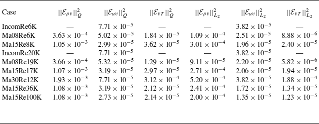
 Eρv=EF[ρ′v″]
 Euv=u″v″~−EF[u″v″]
 EvT=v″T″~−EF[v″T″]
 ||⋅||Q2≡∫02(⋅)2Q(y)dy
 ||⋅||L22≡∫02(⋅)2dy
 u″v″~
u″v″~ v″T″~
v″T″~ uτ=(τw/ρw)1/2
 Tτ=qw/ρwcpuτ
 Mab=1.5
 Reτ=1000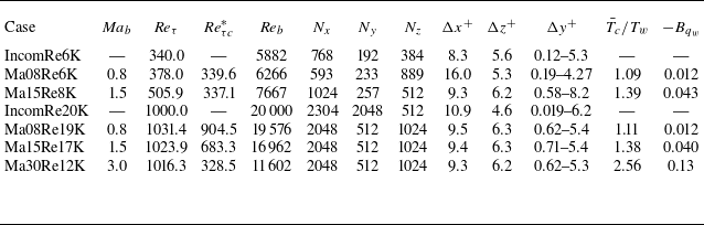
 Lx×Ly×Lz=6πh×2h×2πh
 Lx×Ly×Lz=8πh×2h×3πh
 Lx×Ly×Lz=8πh×2h×4πh
 Lx×Ly×Lz=6πh×2h×2πh
 Nx
Nx Ny
Ny Nz
Nz (x,y,z)
 Δx+
Δx+ Δz+
Δz+ Δy+
Δy+ T¯c/Tw
 Bqw=q¯wm/(cpρwm¯uτTwm)
 qwm
qwm
 Reτ≈1000
 Mab=1.5
 Mab=3.0
 Reτ≈1000
 Mab=
Mab= Mab=3.0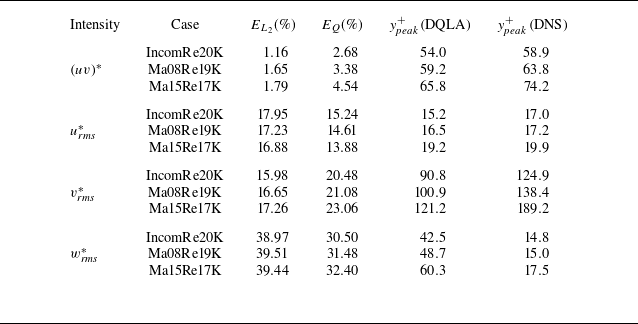
 Reτ≈1000
 uv∗
uv∗ EL2≡100×(∫02(uvDQLA∗−uvDNS∗)2dy/∫02(uvDNS∗)2dy)1/2
 EQ≡100×(∫02(uvDQLA∗−uvDNS∗)2Q(y)dy/∫02(uvDNS∗)2Q(y)dy)1/2
 Reτc∗≈340
 Mb=0.8
 1.5
1.5 3.0
3.0 Mb=0.8
 1.5
1.5
 Reτ=1000
 Mab=0.8,1.5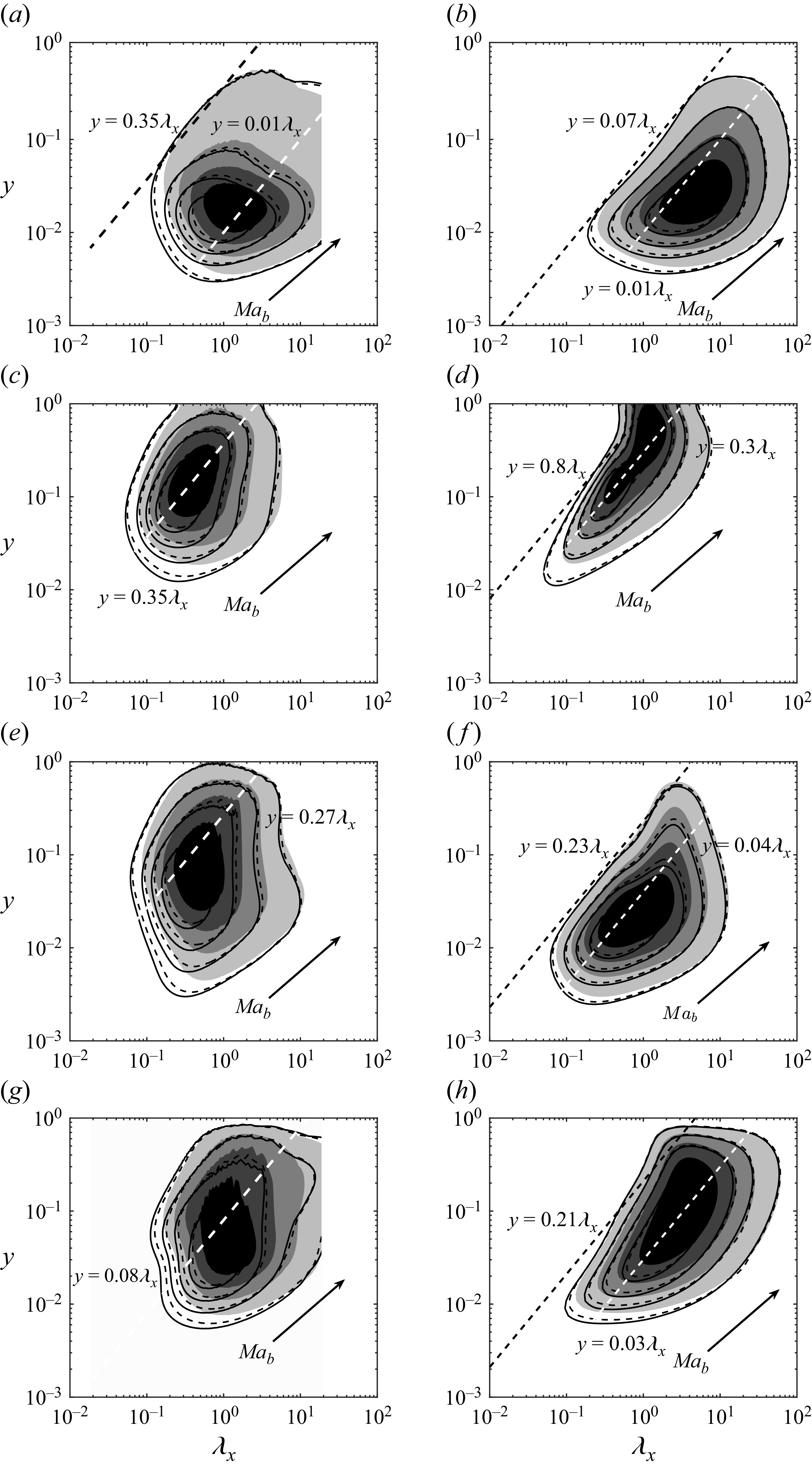
 Reτ=1000
 Mab=0.8,1.5
 Reτc∗≈340
 Mab=0.8
 1.5
1.5
 Reτc∗≈340
 Mab=
Mab= U~TL+
U~TL+
 kx=0
kx=0 λz,c∗=100
 λz=3.7h
 Reτc∗≈340
 Mab=
Mab=
 Mab=1.5
 Reτc∗=337,684,1343
 Reτc∗=145,337,683,1266
 Reτc∗=337,684,1343,3404
 Aln(y)+B
 A=−2.45
 B=0.12
 Reτc∗
Reτc∗ Clog(Reτc∗)+D
 C=1.36
 D=1.83
 u″v″~
u″v″~ v″T″~
v″T″~ Mab=0.8,1.5,3.0
 Reτ=1000
 v″T″~
v″T″~ Mab=0.8
 1.5
1.5 3.0
3.0 Reτ≈1000
 Reτ≈1000
 Mab
Mab NPOD
NPOD NPOD
NPOD NPOD
NPOD
 σj/V
σj/V Mab=
Mab= Reτc∗≈340
 λz,c∗=100
 λz=3.7h
 kx=0
kx=0 kx/kz=0.25
 λz+=100
 λz=3.7h
 Mab=1.5
 Reτ=1000
 y−z
y−z
 Reτ≈1000
 Mab
Mab kzh=14
 30
30 50
50 76
76 126
126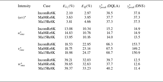
 Reτ∗≈340
 EL2
EL2 EQ
EQ
 Mab=1.5
 EL2
EL2 EQ
EQ
 Reτ∗≈340
 kzh=30
 Mab=0.8
 Mab=1.5
 Open access

