3.1.1. Experimental observations

The spatio-temporal radial development of $u_{\theta }$ , was investigated over a period of 78 s at three different locations and for different angular speeds, in the absence of any fluid discharge, as per the details provided in § 2.2.1. The experimental $u_\theta$ values presented are azimuthally averaged ones, obtained after interpolating the $u_x$ and $u_y$ velocity components from 2-D PIV measurements (see figure 1 a) onto the two in-plane velocity components of a corresponding polar coordinate system.

Figure 2(a) compares the experimentally obtained $u_{\theta }$ distribution (bottom sector), after spatially averaging five repetitions from the 2-D PIV data at $t =78$ s – or, with reference to (3.2), the dimensionless time $t_d={\lambda }^{2}_{1}{ (4\nu {t} )}/{D^{2}_{o}}\approx 4.47$ , where $\lambda _{1}=3.83$ – for the case $\Omega =1.95$ $\,\rm rad\,\rm s^-{^1}$ at $z=-2D_{o}$ , with the expected solid-body rotation distribution (top sector), $u_{\theta }=\Omega {D_{o}}/2$ . The difference between both distributions is clear, especially in the vicinity of tube centre, $r=0$ .

Figure 2(b) shows the temporal evolution of $u_{\theta }$ , for $0 \le r \le D_{0}/2$ and $0 \le t_{d} \le 4.4$ , from which it is clear that for $t_{d}=4.4$ , the corresponding $u_{\theta }$ distribution predicted by (3.2) has already reached a steady state of solid-body rotation, in contrast to that obtained experimentally for the flow inside a rotating tube of finite length, where for $t_{d}\gt 2.7$ $u_{\theta }$ converges to a distribution that is deficient compared with one of a solid-body rotation type.

Figure 2.

(a) Spatial distribution of $u_{\theta }$ in a rotating tube of infinite length predicted by (3.2), namely solid-body rotation (top sector), and obtained experimentally with a tube of finite length (bottom sector); with $\Omega =1.95$ $\,\rm rad\,\rm s^-{^1}$ at $z=-2D_{o}$ and after $t =78$ $\rm s$ from the onset of rotation. (b) Corresponding temporal evolution of $u_{\theta }$ as a function of $r$ at different dimensionless diffusion times $t_d$ : dashed lines (3.2); colour markers, experimental results measured at $z=-2D_{o}$ ; black markers, corresponding numerical predictions (see § 3.1.2).

For $t\lesssim 12$ $\rm s$ ( $t_d\lesssim 0.69$ ), the results obtained experimentally agree well with the predictions of (3.2). However, at larger times, the experimental results for the case of a rotating tube of finite length reveal a lower $u_{\theta }$ , this difference being more pronounced at intermediate $r$ . It is clear from the above that previous experimental work, such as that of Naitoh et al. (Reference Naitoh, Okura, Gotoh and Kato2014), where the preparation time is reported to be 15 $s$ , actually involved the use of a partially established $u_\theta$ velocity distribution in the production of vortex rings.

It is plausible that the boundary condition existing in practice at the two ends of the rotating tube of finite length, with one end open to a large stagnant reservoir and the other essentially a no-slip spinning end wall, has a strong impact on $u_{\theta }$ development. From figure 2(b), subtle discrepancies between measurement and the predictions of (3.2) can be observed at very small time, because of the proximity of the measurement plane to the OEP, suggesting the presence of a secondary flow originating from the difference in pressure at the two ends of the rotating tube of finite length. Due to the inherent difficulty of optical access through two cylindrical Perspex walls, rendering PIV measurement impractical, in order to understand the nature of this secondary flow a complementary axisymmetric direct numerical simulation – as described below – was undertaken.

3.1.2. Numerical predictions

In the absence of an analytic solution for the case of a rotating pipe of finite length – closed at one end and contiguously abutting to a large quiescent fluid bulk at the other – an appropriate model, embodying the essential features of the experimental set-up, was solved numerically using OpenFOAM®. To this end, the nature of the flow can be assumed laminar and incompressible (density, $\rho$ ), and governed by the corresponding continuity and Navier–Stokes equations, namely

(3.3) \begin{eqnarray} \frac {\partial {u_{i}}}{\partial {x_{i}}}&=&0, \end{eqnarray}

(3.4) \begin{eqnarray} \frac {\partial {u_{i}}}{\partial {t}}+u_{j}\frac {\partial {u_{i}}}{\partial {x_{j}}}&=&-\frac {1}{\rho }\frac {\partial {p}}{\partial {x_{i}}}+\nu \frac {\partial ^2{u_{i}}}{\partial {x_{j}}\partial {x_{j}}}, \end{eqnarray}

where $p$ is the pressure. The 2-D computational domain employed, depicted in figure 3, takes the form of an axisymmetric wedge-shaped slice through an equivalent 3-D flow geometry. The latter is comprised of a reservoir of length $ z = 5D_{o}$ and radius $r = 5D_{o}$ , to which a pipe of diameter $D_{o}$ and length $20D_{o}$ is connected with its central axis aligned with the axis of symmetry, forming a simplified swirling ring generator system having an orifice entrance. In order to differentiate between the experimental set-up described in § 2.1 and the simplified model of the same, the term ‘pipe reservoir’ is used instead of ‘tube tank’ for the latter. A no-slip condition is applied at the outer (cylindrical) surface, and at the left closed end, of the pipe. The pipe (surface and closed end) rotates at an angular speed $\Omega$ , based on which the Reynolds number, given ${Re}=D^{2}_{o}\Omega /2\nu , \ \mbox {is}\ \approx 1000$ .

Regarding the specifics of the methods of solution and discretisation, the pressurevelocity coupling algorithm used employs the pressure-implicit with splitting of operators method (Issa Reference Issa1986), with second-order differencing utilised for all the spatial and temporal derivative terms. A time step of $1\times {10^{-4}}$ was employed to ensure that the maximum Courant–Friedrichs–Lewy number remained below 1 for all the flow cases considered.

Figure 3.

(a) Pipe-reservoir computational domain employed to obtain axisymmetric numerical solutions, including a blow-up of the mesh refinement employed at the corner forming an orifice. (b) A contour plot of $u_{z}$ in the pipe and close to the orifice, $t_d = 4.4$ , together with the streamline pattern that forms in the $r-z$ plane of the flow configuration, generated by the rotating pipe. Only the first quarter length of the latter, adjacent to the orifice exit, is shown.

Following a rigorous mesh independence study, the final mesh of choice consisted of a total $153\,000$ structured grid cells, concentrated mainly in the pipe and in the vicinity of the corner/orifice where the pipe connects to the reservoir. The numerical solutions obtained are validated against experimental measurement, in terms of the dependence of $u_\theta$ on $r$ and $t$ , in figure 2(b).

In a rotating system, pressure increases with increasing $r$ from the centre of rotation to balance the centrifugal acceleration. This creates a zone near the rotating surface of the pipe, of higher pressure than that for smaller $r$ and than in the adjoining reservoir where flow is initially irrotational. Consequently, fluid is thus expelled from the pipe at larger $r$ , with fluid from the reservoir close to the pipe exit, or orifice, entrained to replace it, forming a recirculating region which penetrates into the pipe. This behaviour is illustrated in figure 3(b), where to appreciate what is happening, it is only necessary to show the first quarter length of pipe leaving the reservoir. It can be seen from the in-plane streamline pattern that the entrained irrotational flow occupies the central region of the pipe, decreasing $u_{\theta }$ there. The induced secondary flow also gives rise to the extensive slow circulating flow pattern observed in the large reservoir.

The numerical results presented in figure 4(a,b) show that the evolution of $u_{\theta }$ is associated with the transient development of the axial flow pattern inside the pipe, i.e. $u_{z}$ , which is highly time-dependent. The value of $u_{z}$ remains negligible for the first $6$ s, $t_d\lesssim 0.34$ , beyond which it loses uniformity until for $t_d\gt 0.68$ its value becomes appreciably more marked with time. Near the rotating pipe’s bounding surface, $r\gtrsim 0.3D_o$ , $u_{z}\gt 0$ and flow is expelled to the reservoir, while for $0\leqslant r\lesssim 0.3D_o$ , $u_{z}\lt 0$ and fluid from the reservoir is entrained into the pipe.

Figure 4.

Temporal and spatial distributions of $u_\theta$ and $u_z$ within the rotating tube/pipe. Panels show (a) $u_{z}$ predicted numerically and (b) a comparison of $u_{\theta }$ profiles: marker shapes follow the legends in (a), coloured open ones from experiment, those filled and black numerical predictions and the solid line (3.2). (c) Experimentally measured $u_{\theta }$ at $r=D_{o}/4$ , for $z/D_o=-1, -2$ and $-3$ ; legend same as (d). (d) Experimentally measured $u_{\theta }$ at $r=D_{o}/4,z=-2D_{o}$ and for four different tube rotation speeds, where subscript $n=1,2,3,4$ with $\Omega _1=\Omega =1.95$ $\,\rm rad\,\rm s^-{^1}$ , the benchmark rotation speed; $\Delta u_\theta$ is the difference between the measured value and (3.2). In (a)–(d), marker colour differentiates the $z$ coordinate and marker shape differentiates $t_d$ values.

The behaviour of the $u_z$ distribution influences the sectional $u_{\theta }$ profiles, as displayed in figure 4(b). At $t_d=1.37$ , the experimentally determined $u_{\theta }$ profile deviates from the corresponding analytical solution given by (3.2), and to a greater extent closer to pipe exit, or orifice, giving credence to the numerical results. For a clearer comparison, in figure 4(c) $u_\theta$ when $r=D_{o}/4$ is plotted at 3 axial locations and for $t_d=0.68,1.37,2.75$ , together with the value calculated using (3.2). It echoes the finding in figure 4(b) for all three $t_d$ examined; additionally, the degree of deviation is amplified with increasing time.

As demonstrated in § 3.1.3, $u_{z}$ is generated by the difference in pressure at the two ends of the pipe due to it being rotated. Consequently, an increase in $\Omega$ is expected to lead to a non-uniform $u_{z}$ with larger magnitude and hence with a stronger impact on the $u_{\theta }$ distribution. This is established in figure 4(d), which examines $u_{\theta }$ at a single location ( $r=D_{o}/4, z=-2D_o$ ) for four $\Omega$ s. The value of $u_\theta$ on the left-hand side vertical axis is normalised by the benchmark rotation rate ( $\Omega _1=1.95$ $\,\rm rad\,\rm s^-{^1}$ ), enabling direct comparison. Plotted on the right-hand side vertical axis is the (relative) deviation $\Delta u_\theta$ , defined as the difference between the experimentally determined $u_\theta$ and that calculated via (3.2). This figure clearly illustrates significant $u_\theta$ deficit as $\Omega$ increases. It appears that at this particular location, $u_\theta$ saturates at a value of $\Omega _2=3.9$ $\,\rm rad\,\rm s^-{^1}$ for large time. Larger $\Omega$ does not have any effect on increasing $u_\theta$ there, plausibly due to very strong $u_z$ related secondary flow. In line with figure 4(a), the secondary flow needs time to become established. That is, $\Delta u_\theta$ remains small at small time ( $t_d=0.68$ ), increasing subsequently towards steady state.

3.1.3. Simplified model

A simple model is now formulated in order to explain the mechanism by which the secondary flow discussed above arises. That is, to understand the physics behind the particular $u_z$ distribution that develops and the lack of agreement of $u_{\theta }$ with that of a solid-body rotation-like distribution being due to the axial pressure gradient imposed by the boundary conditions at the two ends of the rotating pipe.

The state at large time and an axial location $L_{p}$ far away from where the pipe meets the reservoir is considered. At this location, based on observations with respect to figure 4(c) that the further along the pipe from the OEP that $u_\theta$ is measured, the closer it is to that of a solid-body rotation – the effect of the secondary flow being weak and ${\partial }u_{z}/{\partial }{z}\ll {\partial }u_{z}/{\partial }{r}$ . That is, far away from the OEP, the axial pressure gradient is entirely balanced by viscous effects. Assuming the flow inside the pipe is axisymmetric and the radial velocity component $u_{r}$ is negligible everywhere, the governing momentum equations in cylindrical polar coordinates reduce to

(3.5) \begin{eqnarray} \frac {1}{\rho }\frac {\partial {p}}{\partial {z}}&=&\nu \left (\frac {1}{r}\frac {\partial u_z}{\partial r}+\frac {\partial ^2 u_z}{\partial r^2}\right ), \end{eqnarray}

(3.6) \begin{eqnarray} \frac {1}{\rho }\frac {\partial {p}}{\partial {r}}&=&\frac {{u_{\theta }}^2}{r}. \end{eqnarray}

The boundary conditions which prevail are shown in figure 5(a): (i) $u_\theta (r)=\Omega r$ (solid-body rotation) at $z=-L_p$ , equivalent to a disc at the closed end spinning together with the pipe; (ii) at the OEP, $z=0$ , pressure is zero gauge; (iii) on the surface wall of the rotating pipe, $r=D_o/2$ , a no-slip condition applies, viz. $u_\theta =\Omega D_o/2$ , $u_z=0$ .

Figure 5.

(a) Illustration of the boundary conditions used for the simple model. (b) Comparison of $u_{z}$ profiles obtained numerically with the one given by (3.9).

The $u_z$ distribution inside the pipe shown in figure 4, suggests that, as $r\to D_o/2$ , both the first and the second derivatives on the right-hand side of (3.5) should be negative, implying that so should $\partial p/\partial z$ . On the other hand, (3.6) suggests that to sustain solid-body rotation, $p$ reduces toward small $r$ . Therefore, $p$ is expected to have a positive and maximum value at $z=-L_p,r=D_o/2$ , denoted as $p_{{{max}}}$ . The numerical result indeed confirms this.

Taking the above further, the corresponding derivation is simplified by decoupling the system of equations (3.5)–(3.6). Integrating (3.6), for a velocity distribution satisfying a solid-body rotation at $z=-L_p$ , leads to

(3.7) \begin{equation} p=p_{{max}}-\frac {1}{2}\rho {\Omega }^2\left [(D_{o}/2\right )^2-r^2]. \end{equation}

If the axial pressure gradient ${\partial }p/{\partial }{z}$ is assumed to be independent of $z$ , as a crude assumption

(3.8) \begin{equation} \frac {\partial {p}}{\partial {z}}\simeq \frac {\Delta {p}}{\Delta {z}}=\frac {1}{L_p}\left ({p|}_{0}-{p|}_{L_p}\right )=\frac {1}{L_p}\left \{-p_{{max}}+\frac {1}{2}\rho {\Omega }^2\left [(D_{o}/2)^2-r^2\right ]\right\}. \end{equation}

Now, integrating (3.5) twice, with $\partial u_z/\partial r=0$ , at $r=0$ and $u_z=0$ at $r=D_o/2$ , and making use of (3.8), gives

(3.9) \begin{equation} \frac {u_{z}(r)}{\frac {1}{2}\Omega D_o}=Re \left (\frac {L_p}{D_o}\right )^{-1}\left \{\frac {1}{8}\left [\left (\frac {r}{D_o}\right )^2-\left (\frac {r}{D_o}\right )^4-\frac {3}{16}\right ]+\tilde {p}\left [\frac {1}{4}-\left (\frac {r}{ D_o}\right )^2\right ]\right\}, \end{equation}

where $\tilde {p}=p_{{max}}/ (\rho \Omega ^2 D_o^2 )$ and $R{e}={D_{o}^{2}\Omega }/2\nu$ .

The distribution of $u_{z}$ calculated using (3.9), with $L_p/D_o=10$ and setting $\tilde {p}\approx 0.08$ – its value obtained numerically – together with numerically generated counterparts at different $z$ locations along the pipe from the orifice exit are compared in figure 5(b).

It can be seen that this simple model captures the characteristics of the $u_z$ distribution, which includes a suction region at small $r$ and expulsion region at large $r$ . The chosen parameters coincidentally describe the $u_z$ distribution at $z\approx -3D_{o}$ .

As suggested by (3.9), the exact distribution of $u_{z}$ depends on the value of $Re$ , $L_p/D_o$ and $\tilde {p}$ . Since $\tilde {p}$ typically has a value around $0.08$ over a physically reasonable range, with $u_z\lt 0$ at small $r$ , $\partial u_z/\partial r$ and $\partial ^2 u_z/\partial r^2$ are both negative approaching the rotating wall of the pipe. The $r$ coordinate, where $u_z$ approaches a maximum, decreases as $\tilde {p}$ increases. For a given $\tilde {p}$ , as $L_p/D_o$ increases the $u_z$ distribution becomes more uniform – i.e. the effect of the secondary flow diminishes which is consistent with experimental observations and what is calculated numerically.

It is important to stress that this simplified model is only meant to be qualitative, since it does not impose a zero mass flux associated with the $u_z$ distribution at any cross-section. Nevertheless, it is insightful in showing that it is the axial pressure gradient which induces the observed secondary flow pattern.

Accordingly, the flow of interest can be considered a combination of that inside an infinitely long rotating tube described by (3.2) and that induced by a rotating disk of large diameter (von Kármán flow), and governed by second-order nonlinear partial differential equations having a self-similar solution but not in an explicit form (Batchelor Reference Batchelor1967). For large time when the flow’s dependence on time becomes negligible, $u_\theta$ can be described approximately by the following empirical relationship:

(3.10) \begin{equation} u_{\theta }(r,z)=\Omega {r}+\Omega {D_{o}}\sum ^{\infty }_{n=1}\displaystyle \frac {J_{1}\left (\lambda _{n}\frac {2r}{\,D_{o}}\right )}{\lambda _{n}J_{0}(\lambda _{n})} \mathrm {exp}[g\!\left(z\right ){\lambda }_n^{2}]. \end{equation}

The form of the above, which is analogous to (3.2), stems from the observed similarity between the temporal evolution of $u_\theta$ at a fixed distance, $z = -2D_{0}$ , into the rotating tube from the OEP (figure 2 b) and the nature of $u_\theta$ at the same $t_{d} = 1.37$ at different distances, $z = -D_{0}, -2D_{0}, -3D_{0}$ into the tube (figure 4 b); i.e. $g\to -\infty$ as $z\to -\infty$ , and $u_\theta$ approaches one of solid-body rotation.

A least squares fitting for $u_\theta$ over $-10\leqslant z/D_o\leqslant 0$ , yields the plot of $g(z)$ against $z/D_{0}$ shown in figure 6(a), allowing the relationship between the two to be expressed in dimensionless form, but not uniquely, by

(3.11) \begin{equation} g(z)=\frac {1.68\times 10^{-2}}{1.13-\exp \left [0.19\left ({z}/{D_o}\right )\right ]}\left (\frac {z}{D_o}\right ). \end{equation}

Figure 6.

(a) Dependence of $g$ on $z$ ; markers are from fitting numerically generated values of $u_\theta (r,z)$ at large time ( $t_d=3.4$ ) with (3.10), each for a discrete $z$ , while the solid line results from (3.11) itself. (b) Dependence of $u_\theta$ on $r$ for $z/D_o\geqslant -10$ ; markers indicate numerically generated results while solid lines of the same colour result from (3.10).

Figure 6(b) demonstrates that the $u_\theta (r,z)$ profiles predicted at large time are well described by (3.10) over the first $10D_o$ of the pipe, except very close to the OEP due to the contiguous presence of the large reservoir. The agreement between numerical prediction and experiment is confirmed in figure 2(b). Flow further into the pipe is less relevant to the work of interest here due to the short $L/D_o$ involved.

3.2.1. Opposite-signed vorticity and circulation

Figure 7 shows the individual velocity contours of the three velocity components inside the rotating pipe close to the OEP, obtained from the axisymmetric numerical solution at $t_d\approx 3.95$ ( $t=70$ $\rm s$ ) – at which time flow inside the pipe is considered fully established. It is plausible to assume they represent the distribution of velocity inside the rotating tube commensurate with corresponding experiments, even though the boundary condition at the closed end of the tube does not, in practice, match exactly that of the computational predictions. Reassurance of this comes from the agreement between prediction and experimental data in terms of the $u_\theta$ profiles shown in figure 2(b). Note also that $u_r$ is an order of magnitude smaller than $u_\theta$ and $u_z$ , and therefore its effect can indeed be neglected. The $z$ range plotted in figure 7 corresponds approximately to the fluid material discharged, since $L/D_o=2$ .

Figure 7.

Numerically predicted velocity contours in the region bounded by the OEP ( $z = 0$ ) and at a distance $z = -2D_{0}$ into the rotating pipe, when $t=70$ $\rm s$ ( $t_d\approx 3.95$ ). Panels show (a) $2u_\theta /(\Omega D_o)$ , (b) $2u_z/(\Omega D_o)$ , (c) $2u_r/(\Omega D_o)$ . The corresponding value of $\Omega$ is 1.95 $\rm rad\,s^{-1}$ , with $0.5\Omega D_o\approx U_o$ . Note the different scales for the $z$ and $r$ axes.

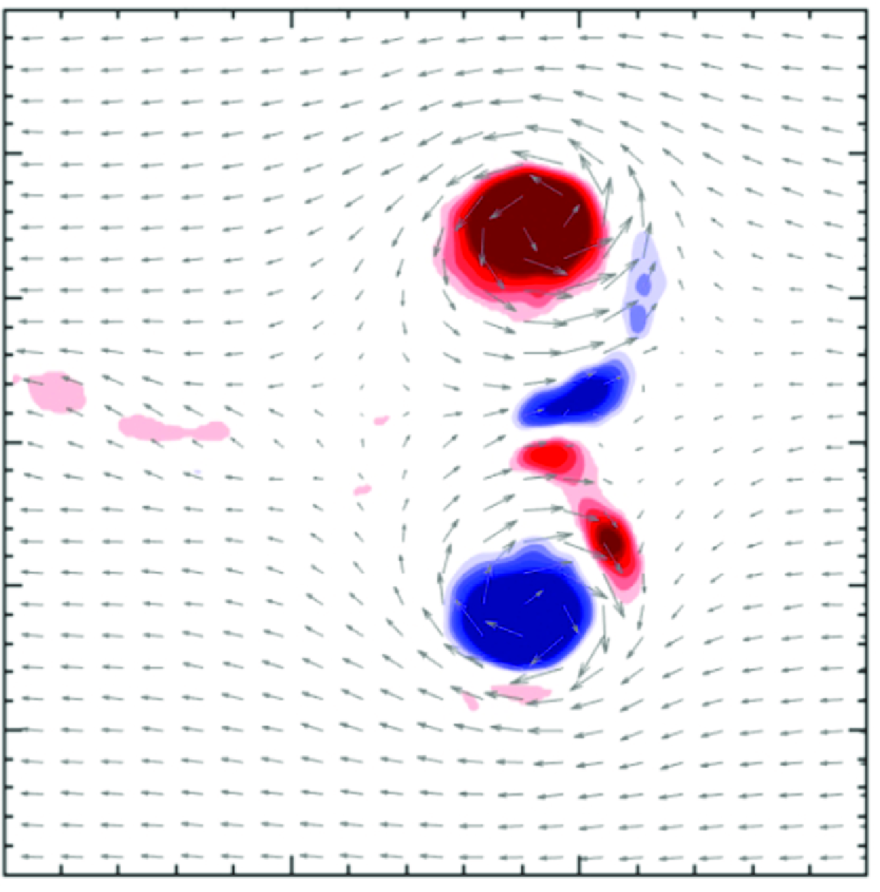
The in-plane velocity vectors $ (u_z,u_y )$ and the contours of the out-of-plane vorticity, $\omega _x$ , acquired by PIV are shown in figures 8(a), 8(b) and 8(c) for $S=0.25,$ $0.5$ and $1$ , respectively. The value of $\omega _x=\partial u_{y}/\partial {z}-\partial u_{z}/\partial {y}$ , calculated from $ (u_z,u_y )$ by applying a central difference scheme, is equivalent to the azimuthal vorticity $\omega _\theta$ if the problem is cast in terms of cylindrical coordinates. The difference in OSV production is evident, particularly between the cases $S=0.25$ and $0.5$ , with regions of vorticity of opposite sign to that of the adjacent primary vortex appearing around the vortex ring core towards the centre. Its formation originates from vortex breakdown – i.e. the tilting of $\omega _x$ associated with the distribution of $u_{\theta }$ – and can be derived from the azimuthal component of the inviscid vorticity equation (Ortega-Chavez et al. Reference Ortega-Chavez, Gan and Gaskell2023) to be

(3.12) \begin{equation} \frac {\partial \omega _x}{\partial t}=\frac {1}{2}\frac {\partial }{\partial {z}}\left (\frac {{u_{\theta }}^2}{r}\right ). \end{equation}

This is the reason the OSV intensity would be even higher close to the centre of the swirling ring, if the generated swirl were of a solid-body rotation type.

What is observed in figure 8 is consistent with the above, notwithstanding the non-solid-body rotation type of swirl involved. Although the OSV is weak for $S=0.25$ , its location is close to the axis. For $S=0.5$ and $1$ , OSV is produced near the axis and advected around the primary vortex core in accordance with the induced velocity generated by the vortex ring, interacting with it and causing destabilisation and vorticity cancellation. On closer inspection of the velocity vectors in the central region along $y=0$ , vortex breakdown is observed. Here, velocity vectors are presented in a moving frame of reference travelling together with the primary vortex core in the $+z$ direction. In this frame of reference, the windward stagnation point (s.p.), where the velocity reduces to zero, is marked for each case. In figure 8(a), the s.p. is located upstream of the vortex core, marking the position of the vortex ring bubble boundary on the central axis. As $S$ increases, figures 8(b), the s.p. shifts to a more downstream location relative to the primary ring core, and to even behind the vortex core in (c) due to a stronger vortex breakdown effect. Figure 8 also shows that OSV induces a subtle effect to the shape of the primary ring core. Increased $S$ reduces the core size, making it more circular, consistent with the result commensurate with a $u_\theta$ of a solid-body rotation type as investigated in Ortega-Chavez et al. (Reference Ortega-Chavez, Gan and Gaskell2023).

Figure 8.

Contours of $\omega _x$ with background velocity vector at $T^{*}=5$ for (a) $S=0.25$ , (b) $S=0.5$ and (c) $S=1$ . A threshold of $|\omega _x|\gt 1$ $\rm s^{-1}$ is applied. The velocity vectors are associated with a frame of reference moving at the instantaneous propagation velocity of the primary vortex core in the $z$ dirction, from which the windward s.p., marked by a filled square box, can be identified.

Figure 9(a) compares the circulation associated with OSV, denoted as $\Gamma (OSV)$ and calculated by integrating the area occupied by the OSV, $A(OSV)$ . Namely

(3.13) \begin{equation} \Gamma (OSV)=\frac {1}{2}\int _{A(OSV)}\left [\omega _x({-})-\omega _x({+})\right ]\;\mathrm {d}A. \end{equation}

A threshold $|\omega _x|\gt 1$ $s^{-1}$ is applied to remove background noise and the dimensionless form of the above given by $\Gamma ^*=\Gamma / (U_oD_o )$ ; $A(OSV)$ , where $\omega _x$ is generated by the interaction between the primary vortex ring and the orifice wall, which has the same sign as OSV, is excluded from (3.13). The magnitude $|\Gamma (OSV)|$ increases (the OSV is more negative) with increasing $S$ , and for $S=1$ , $|\Gamma (OSV)|$ is a maximum for $T^{*}=tU_o/D_o\lesssim 4$ . For $T^{*}\gt 5$ a faster decrease in $|\Gamma (OSV)|$ is observed, which is likely related to stronger interaction with the primary vortex ring, leading to significant vortex cancellation. As a result the value of $|\Gamma (OSV)|$ eventually becomes even lower than what is observed for the case $S=0.5$ . On the other hand, for $S=0.25$ and $0.5$ , $|\Gamma (OSV)|$ continues increasing until ${T^{*}}\approx 5.5$ , and then decreases very gently.

Figure 9.

(a) Evolution of the dimensionless circulation associated with OSV. (b) Dimensionless OSV circulation normalised by $S^2$ (Ortega-Chavez et al. Reference Ortega-Chavez, Gan and Gaskell2023). (c) Evolution of the dimensionless primary ring circulation $\Gamma ^{*}_{Ring}$ . For all the cases, a threshold of $|\omega _x|\gt 1$ $\rm s^{-1}$ was applied.

The numerical work of Ortega-Chavez et al. (Reference Ortega-Chavez, Gan and Gaskell2023) showed, for moderate $S$ , that $\Gamma (OSV)$ in rings produced with $L/D_o=6$ scales with $S^{2}$ as a consequence of (3.12). In figure 9(b), the effect of scaling by $S^2$ is reasonably well captured for the cases $S=0.25$ and $0.5$ . The $S=1$ case only behaves similar to the previous two for $T^{*}\lesssim 4$ ; beyond that, it deviates significantly from the other cases. These discrepancies may be attributable to the following factors.

1. (i) Firstly, in the current work, $L/D_o=2$ ; typically smaller than the formation number $F$ . Isolated rings without a jet-like wake are formed. For $T^*\gt 2$ no further continuous momentum is delivered from the tube to sustain vortex tilting in the region close to the ring’s axis. In turn, vorticity cancellation dominates over the OSV production rate affecting the $S^2$ scale.

2. (ii) Secondly, as detailed in § 3.1, the difference in boundary condition at the two ends of a rotating tube of finite length induces a secondary flow, prohibiting full establishment of a solid-body rotation, which consequently reduces the total swirl momentum flux, and subsequently hinders the production of OSV via diminishing $\partial (u_{\theta }^2/r )/\partial {z}$ . This swirl flux deficit increases with $S$ .

Increase of vorticity cancellation with $S$ can also be observed through the simultaneous decrease of the primary ring circulation, $\Gamma _{Ring}$ , calculated using (3.13) and integrating over the area occupied by the primary vortex. Figure 9(c) compares the time evolution of $\Gamma _{Ring}$ . In all cases, decay of $\Gamma ^{*}_{Ring}$ is evident. For the non-swirl case, $S=0$ , decay is expected to be a consequence of viscosity dissipation, and therefore the more rapid decay rates reflected when $S\gt 0$ can be attributed to cancellation between ring vorticity and OSV. For $T^{*}\gtrsim 6$ , the increased rate of decline when $S=1$ indicates stronger interaction, consistent with figure 9(a). To aid comparison, $\Gamma ^{*}_{Ring}$ is fit to a linear function of $T^*$ , viz. ${\rm d} \Gamma ^*_{Ring}/{\rm d}T^*$ averaged over the scrutinised period; although careful inspection suggests that $\Gamma _{Ring}$ decay should be governed by a more complex function – i.e. $\Gamma _{Ring}$ falls off more rapidly at smaller than at large $T^*$ when $\Gamma (OSV)$ approaches zero.

3.2.2. Ring size and propagation velocity

Convection of OSV to the primary vortex core area results in an upstream translation of the windward s.p. in a frame of reference moving downstream at a velocity equal to the propagation velocity of the ring core, $u_z^\prime$ , figure 8. This translation is absent in the case of a non-swirling vortex ring. According to the Biot–Savart law (Brown & Lopez Reference Brown and Lopez1990; Ortega-Chavez et al. Reference Ortega-Chavez, Gan and Gaskell2023), this upstream movement promotes vortex breakdown which, consistent with the continuity equation, also enhances the radial velocity of the vortex ring – i.e. expansion of the ring radius $R$ , which is shown in figure 10(a). $R$ was determined using the vortex core centroids defined as follows:

(3.14) \begin{equation} R=\frac {\displaystyle \iint \omega _x{y}\;\mathrm {d}y\mathrm {d}z}{\displaystyle \iint \omega _x\;\mathrm {d}y\mathrm {d}z} \quad Z=\frac {\displaystyle \iint \omega _x{z}\;\mathrm {d}y\mathrm {d}z}{\displaystyle \iint \omega _x\;\mathrm {d}y\mathrm {d}z}. \end{equation}

Figure 10.

(a) Ring radius $R$ at $T^*_1=2.5$ . (b) Evolution of $R$ . (c) Dimensionless ring propagation velocity $\Phi$ . Legend as in figure 9(c).

Figure 10(a,b) demonstrates that swirl has a clear effect on the size of the primary ring at two stages of its evolution. The first stage is the formation process revealed by figure 10(a). At $T^*_1=2.5$ , soon after discharge stops and when the ring pinches off, larger $S$ results in a larger sized ring being formed – probably from a combination of centrifugal and OSV effects imposed by the swirl during roll-up of the primary vortex core. Subsequently, rings for the different $S$ cases experience a short transient period for $2.5\lesssim T^*\lesssim 3.4$ , when similar behaviour with respect to $R$ is observed. For the second stage, $T^*\gt 3.5$ , $S$ effect becomes distinguishable again, figure 10(b). Here, larger $S$ leads to a greater growth rate for $R$ . The behaviour of $R$ is related to the vortex breakdown process induced by the $u_\theta$ component and OSV, which can be inferred from the behaviour of $\Gamma (OSV)$ in figure 9. That is, the cumulative effect of larger $|\Gamma (OSV)|$ results in a greater growth rate of $R$ . Further evidence is presented in § 3.3.2.

A subtle increase in the extent of the waviness of $R$ with $S$ is also seen. This is likely due to core instability in the form of azimuthal waves (Maxworthy Reference Maxworthy1977), which is promoted by the interaction between the primary ring core and OSV. These core waves also rotate about the ring axis under the effect of azimuthal velocity $u_\theta$ . It is worth remembering that rings may have drifted out of the measurement plane slightly as time passed, which might be the reason for the small decrease of $\Delta R\sim 0.02D_o$ for the case $S=0$ .

Figure 10(c) shows the normalised propagation velocities, $\Phi$ , calculated via the ring core trajectory, and hence $u_z^\prime$ , as

(3.15) \begin{equation} \Phi =u_{z}^\prime \left (\frac {\Gamma _{{Ring}}}{4\pi {R}}\right )^{-1}. \end{equation}

It reveals that over the period scrutinised, $\Phi$ is fairly stable for all $S$ , suggesting that $\Gamma _{{Ring}}/R$ dominates over $u_{z}^\prime$ . For $S=0$ and $1$ , $\Phi \approx 3$ , and $\Phi$ decreases appreciably with increasing $S$ . According to Saffman (Reference Saffman1995), $\Phi$ describes properties of an isolated vortex ring core, as follows:

(3.16) \begin{equation} \Phi ={\ln \left (\frac {8}{\epsilon }\right )} +\frac {1}{\Gamma _{{Ring}}^{2}} \int _{0}^{a}\frac {\gamma ^2(r')}{r'}\;\mathrm {d}r'-\frac {8{\pi }^2}{\Gamma _{{Ring}}^{2}}\int _{0}^{a}u_\theta ^2r\;\mathrm {d}r'-0.5, \end{equation}

where

(3.17) \begin{equation} \gamma (r')=2{\pi }\int _{0}^{a}{\omega }r'\,\rm dr', \end{equation}

with $r'$ being the radius in a local coordinate system with its origin at the vortex core centroid, $\epsilon =a/R$ being the ratio of the primary ring core radius $a$ to the ring radius $R$ , which decreases with increasing $S$ (Ortega-Chavez et al. Reference Ortega-Chavez, Gan and Gaskell2023). The first three terms on the right-hand side of (3.16) take into account the effect of the ring core size, the detailed distribution of $\omega _x$ inside the core via $\gamma (r')$ and the swirl velocity $u_\theta$ in the core, respectively. The inverse dependence of $\Phi$ on $S$ shown suggests that $\Phi$ is predominantly influenced by the decay of $\Gamma _{{Ring}}$ , as presented in figure 9(c).

3.2.3. Azimuthal velocity $u_{\theta }$

During the process of ring formation, $u_{\theta }$ is transported by the rolling up of the vortex sheet (boundary layer) from the rotating tube to the vortex core. No significant trailing jet (fluid with non-trivial out-of-plane vorticity $\omega _x$ ) is formed in this process because of the relatively small $L/D_o$ . Figure 11(a–c) show contours of $u_\theta$ at $T^*=4$ , long after formation is completed and ring bubble pinched off has occurred; compare this with the $\omega _x$ contours in figure 8 at the later time $T^*=5$ . Here, the $u_\theta$ distribution is the average of the in-plane upper and lower vortex ring segments.

Figure 11.

(a–c) The $u_{\theta }$ distribution at $T^{*}=4$ for $S=0.25$ , $0.5$ and $S=1$ , respectively. Contour line superposed is at level $\omega _x^{max}(T^*)e^{-1}$ , which marks the primary vortex core. Red lines, which mark the bubble area, are the in-plane streamlines in the frame of reference translating with the vortex core at the instantaneous velocity $u'_{\!\!z}$ . (d) Evolution of spatially averaged $u_{\theta }$ in the vortex core area. (e) Distribution of $\omega _x$ and $u_{\theta }$ along the $y$ and $z$ direction through the $\omega _x$ -based vortex core centroid for the case $S=1$ , where $y_c$ and $z_c$ are in a local coordinate system having its origin at the vortex core centroid, as illustrated in (c).

The above shows that $u_\theta$ is not concentrated in the vortex core area. Instead, it occupies space in the ring bubble and in the wake. The former is the residual swirling fluid that is not entrained into the ring core and transported along with it; the latter is the trace induced and left behind by the ring after it has passed by, which appears as a swirling wake that gets stretched by $\Gamma _{{Ring}}$ induced velocity. The wake-like part is especially clear for the lowest $S$ case, figure 11(a), but different from a formation wake produced when $L/D_o\gg \mathrm {F}$ . A formation wake is indicative of significant $\omega _x$ , which is absent in the current cases; cf. Figure 8.

Only insignificant swirl fluid enters the ring core area. The relationship between $\omega _x$ and $u_\theta$ is shown in figure 11(e) for $S=1$ , at $T^*=3$ and $T^*=5$ (cf. figure 8 c), centred at $T^*=4$ (cf. figure 11 c). A local coordinate system $(y_c,z_c)$ centred at the (moving) $\omega _x$ -based vortex core centroid is utilised. The equivalent vortex core radius $a$ is obtained after applying the threshold $\omega _{x}\geqslant \omega _{x}^{{max}}e^{-1}$ , where $\omega _{x}^{{max}}$ is the peak $\omega _{x}$ at a given time. The $\omega _x$ profile for both $T^*$ remains Gaussian-like in the core area, $-a\lesssim (y_c,z_c)\lesssim a$ , with those along $y_c$ and $z_c$ in good agreement – notwithstanding the influence of $u_\theta$ and OSV (shown as $\omega _x\lt 0$ ), which impose an adverse effect on the core size as shown in (a–c).

The dependence of the $u_\theta$ profiles on $T^*$ reflects a dynamic engulfing process, which reveals the dominant mechanism by which $u_\theta$ gets into the core area. That is, $u_\theta$ is mainly convected by the vortex core induced velocity. Viscous diffusion of $u_\theta$ , evident in Ortega-Chavez et al. (Reference Ortega-Chavez, Gan and Gaskell2023), during the formation process is not clear, plausibly due to the associated small slug length $L/D_o$ .

The swirl velocity in the vortex core, denoted by $\langle u_{\theta } \rangle$ , is quantified by the spatially averaged $u_{\theta }$ in the ring core of equivalent radius $a$ . (Angled braces are used to denote spatial averaged quantities.) Results are presented in figure 11(d) for the $S\gt 0$ cases. When compared with the findings of Ortega-Chavez et al. (Reference Ortega-Chavez, Gan and Gaskell2023) for the case of a solid-body rotation for $u_\theta$ and $L/D_o=6$ , similarities can be observed. Firstly, smaller $S$ is more capable of engulfing swirling fluid material into the core region, but the highest $\langle {u_\theta }\rangle$ attainable in the ring core area is only approximately $0.4SU_o$ which is slightly less than that for the solid-body rotation case. Secondly, $u_\theta$ decays only subtly after the ring pinches off for the case $S=1$ . For the smaller $S$ cases no such decay is apparent; instead $\langle u_{\theta } \rangle$ increases slightly until $T^*\approx 5$ . It echoes figure 11(e) that the engulfment of $u_\theta$ from the region appearing around the primary vortex core towards the centre of the ring axis (see figure 8) dominates over the viscous diffusion effect.

In comparison, $u_\theta$ delivered to the ring core area from the rotating tube is much weaker than the velocity generated by the linear impulse, which is associated with $\Gamma _{Ring}$ . This can be seen from the characteristic velocity $u_c$ of a fluid particle rotating around the vortex core projected in the $y_c-z_c$ plane, which can be written as

(3.18) \begin{equation} \frac {u_c}{U_o}=\frac {1}{\pi }\left (\frac {D_o}{2a}\right )\Gamma ^*_{{Ring}}. \end{equation}

In the above, $\Gamma ^*_{{Ring}}$ and $D_o/a$ can be inferred from figures 9(c) and 8, respectively. Thus $u_c/U_o=\mathcal {O}(1)$ , as expected, whilst $\langle u_{\theta } \rangle /U_o$ is shown to be an order of magnitude lower. In terms of dimensionless time $\tau _\theta$ (scaled by $D_o/U_o$ ), it can be shown for a fluid particle inside the core area to make a full revolution due to $u_\theta$ about the ring axis ( $z$ axis) that

(3.19) \begin{equation} \tau _\theta =\left (\frac {\pi }{S}\right )\left (\frac {2R}{D_o}\right )\left (\frac {u_\theta }{SU_o}\right )^{-1}. \end{equation}

Considering that $R$ increases over time, the strongest swirl case tested $(S=1)$ , leads to $\tau _\theta \sim 20$ . For lower $S$ , $\tau _\theta$ is even larger. This means that for the entire life of the ring, by the time the ring is largely dissipated by viscosity, only approximately 1–2 revolutions will have been completed.

3.3.1. Preparation time

A vortex ring forms as the consequence of a cylindrical-shaped vortex sheet rolling up. In a piston–tube system, this vortex sheet originates from the boundary layer that develops on the inner wall of the tube during discharge. For a swirling vortex ring, the azimuthal velocity $u_\theta$ in the vortex core is also from the portion of $u_\theta$ in this boundary layer, due to the rotating tube, which is then transported by the vortex sheet and engulfed into the core central area. This process, explored in detail in Ortega-Chavez et al. (Reference Ortega-Chavez, Gan and Gaskell2023), can also be inferred from figure 11. The boundary layer thickness occupies roughly the outer 20% of the tube radius (Didden Reference Didden1979), while $u_\theta$ discharged from the central part of the tube is responsible for vortex tilting and vortex breakdown.

It is shown via (3.2) that establishment of $u_\theta$ is initiated at the tube’s inner wall and requires a time scale $D_o^2/\nu$ – referred to subsequently as the “preparation time” for swirl to diffuse to the tube axis. For an infinitely long tube of the same $D_o$ utilised in the present work, it takes of the order of 60 $\rm s$ physical time ( $t_d\approx 3.4$ ) to reach a state of nearly solid-body rotation. It is therefore possible to produce swirling rings with a similar magnitude of $\langle u_{\theta } \rangle$ in the core to those discussed in § 3.2, by reducing this preparation time at a fixed $\Omega$ for a partially established $u_{\theta }$ profile. At the same time, $u_{\theta }$ closer to the tube central region will also be partially established in proportion, which will then reduce the formation of OSV and diminish the degree of breakdown of the primary ring.

To quantify the above the average value of $u_{\theta }$ for the domain $0.4\leqslant r/D_{o}\leqslant 0.5$ was calculated, using (3.2), as

(3.20) \begin{equation} \langle u_{\theta }^p (t)\rangle =2\left [\left (0.5\,D_o\right )^2-\left (0.4D_o\right )^2\right ]^{-1}\int ^{0.5D_{o}}_{0.4D_{o}}u_{\theta }(r,t)r\;\mathrm {d}r. \end{equation}

In what follows, $\langle u_{\theta }^p (t)\rangle$ is denoted as $\langle u_{\theta }^p\rangle$ and explicitly time-dependent. The shaded area in figure 12(a) denotes the range of integration in (3.20). $u_{\theta }$ profiles at $t=6$ and $24$ $\rm s$ are shown, which correspond to $t_d=0.34$ and $1.36$ , respectively, while the experimentally measured $u_\theta$ taken at $z=-D_o$ is used to approximate $u_\theta$ for the entire discharged fluid volume. Although $u_\theta$ is demonstrated in § 3.1 to be appreciably $z$ -dependent, in particular figure 4, $z=-D_o$ is the middle section of the volume discharged and therefore the approximation is expected to be reasonable. For $0.4\leqslant r/D_{o}\leqslant 0.5$ , where $\langle u_{\theta }^p\rangle$ is quantified, the $u_\theta$ value produced by the rotating tube of finite length agrees reasonably well with the theoretical secondary flow free solution, (3.2), especially at early time.

Figure 12.

(a) Comparison between $u_{\theta }$ profiles from experiments measured at $z=-D_o$ , $\Omega =1.95$ $\,\rm rad\,\rm s^-{^1}$ $(S =1)$ and that based on (3.2), at $t_d=0.34$ ( $t=6$ $\rm s$ ) and $1.36$ ( $24$ $\rm s$ ). The shaded area represents $\langle u_{\theta }^p\rangle$ averaged over $0.4\leqslant r/D_{o}\leqslant 0.5$ according to (3.20). (b) The evolution of $\langle u_{\theta }^p\rangle$ in physical preparation time; the second abscissa is the corresponding diffusion time $t_d$ . The vertical dashed lines mark $\langle u_{\theta }^p\rangle$ values at $t=5$ and $20$ $\rm s$ .

Figure 12(b) shows the dependence of $\langle u_{\theta }^p\rangle$ on preparation time; it increases rapidly in the first 10 s ( $t_d\lesssim 0.57$ ), flattening out after 20 $\rm s$ ( $t_d\gtrsim 1.15$ ). For the theoretical case described by (3.2), in steady state $u_{\theta }=\Omega r$ , $\langle u_{\theta }^p\rangle \approx 0.45\Omega D_o=0.9SU_o$ , which is $0.9U_o$ (since $S=1$ ). Half of this value, $0.45SU_o$ , is also delineated in figure 12(b), which only takes roughly $2$ $\rm s$ ( $t_d\approx 0.11$ ) preparation time to achieve. The value of $\langle u_{\theta }^p\rangle$ from experiment is provided for comparison as well, which shows a lower magnitude than predicted by (3.2) due to the presence of secondary flow. Nevertheless, the trend is similar. In particular, the difference in $\langle u_{\theta }^p\rangle$ between $t=5$ $\rm s$ ( $t_d\approx 0.29$ ) and $20$ $\rm s$ ( $t_d\approx 1.15$ ), labelled as $\varDelta$ , shows a similar value for both experiment and theory. This lends support to the impact of preparation time in practice being reasonably quantifiable using (3.2).

It can thus be construed that $S$ is not the only parameter to characterise the swirl strength in a ring produced by a rotating tube as such. The preparation time is the other important parameter. That is, the transient build-up of swirl velocity near the tube’s inner wall, similar to $\langle u_{\theta }^p\rangle$ calculated via (3.20), plays an equally important role to that of $S$ , which must be taken into consideration.

3.3.2. Effect of preparation time on ring properties

Experiments were performed to explore the effect of preparation time $t=0,$ $5,$ $10,$ $15$ and $20$ $\rm s$ ( $t_d\approx [0:0.29:1.15]$ ) on vortex rings with $\Omega =1.95$ $\,\rm rad\,\rm s^-{^1}$ ( $S=1$ ). The outcomes are compared with that for a preparation time of $t=75$ $\rm s$ ( $t_d\approx 4.3$ ), viz. the fully established $S=1$ case discussed in § 3.2, with all the other parameters remaining the same. Note that the preparation time of concern here is the time before the start of the piston stroke, which itself takes approximately 2 $\rm s$ . During this stroke time, swirl continues to develop in the rotating tube and as such the actual swirl delivered by the total fluid discharge will be slightly higher. The stroke time is excluded from the termed preparation time for reasons of simplicity. Zero preparation time, which refers to the case where the onset of the tube rotation synchronises with the piston stroke, is included to evaluate the effect of swirl developed during the duration of the 2 $\rm s$ piston stroke.

Resultant $\omega _x$ contours are shown in figure 13(a), for the minimum $5$ $\rm s$ preparation time ( $t_d\approx 0.29$ ), where no OSV formation can be observed. For zero preparation time, no visible difference can be noticed, the same as for the non-swirl vortex ring ( $S=0$ ); figures not shown. This justifies the amount of swirl issued from the rotating tube during the piston stroke time being taken as unimportant. After 10 $\rm s$ preparation time ( $t_d\gtrsim 0.57$ ), figure 13(b), the presence of OSV becomes observable, and increasingly evident at longer preparation times, figure 13(c,d).

Figure 13.

Contour plots of $\omega _x$ at $T^{*}=4$ , after averaging the upper and lower halves of the associated flow fields. Panels (a)–(d) are for preparation times $5$ , $10$ , $20$ and $75$ $\rm s$ ( $t_d\approx 0.29, 0.57, 1.15$ and $4.3$ ), respectively, with a pipe angular speed $\Omega =1.95$ $\,\rm rad\,\rm s^-{^1}$ $(S = 1)$ . In-plane streamlines in the frame of reference translating in the $z$ direction at $u'_{\!\!z}$ have been superposed to delineate the vortex bubble area.

The value of $\langle u_\theta \rangle$ in the core area is found to be relatively constant for $T^*\leqslant 5$ , regardless of preparation time (figure not shown), which is similar to that of a fully prepared ring shown in figure 11(d). For $T^*\gt 5$ , the interaction between the primary vortex core and OSV is stronger, destabilising the former.

To further facilitate comparison, the time average of $\langle u_\theta \rangle$ , denoted as $\langle \overline {u_\theta }\rangle$ , from the experimental measurements for $2.5\leqslant T^*\leqslant 5$ , is calculated and the results provided in table 1. It can be seen that both $\langle \overline {u_{\theta }}\rangle$ and $\langle u_{\theta }^p\rangle$ have the largest increment from 0 to 5 $\rm s$ preparation time, corresponding to $0\lesssim t_d\lesssim 0.29$ . The non-zero measured $\langle \overline {u_{\theta }}\rangle$ for zero preparation time originates from the swirl input during the $2$ $\rm s$ piston stroke. After 5 $\rm s$ preparation time, $t_d\gt 0.29$ , the increment rate drops appreciably. For instance, $\langle \overline {u_{\theta }}\rangle$ for a zero preparation time is $\approx 30\,\%$ of the $S=0.25$ fully established case. It thus echoes the finding in figure 12(b) that the most efficient swirl delivery to the primary ring core area occurs at small preparation times.

Table 1.

Dependence of the azimuthal velocity magnitude on the dimensional preparation time (Prep. $t$ ), and the corresponding dimensionless diffusion time $t_d$ , for $S=1$ . $\langle \overline {u_{\theta }}\rangle /U_o$ : spatial- and time-averaged azimuthal velocity in the primary ring core based on experiments; $\langle u_{\theta }^p\rangle /U_o$ quantified by (3.20); $\langle u_{\theta }^p\rangle$ from experiment, which can be inferred from figure 12(b), are not tabulated. The results included in the last two columns are for the case $S=0.5$ and $S=0.25$ , both at 75 s $\rm s$ preparation time.

Table 1 also shows that, even though $\langle u_{\theta }^p\rangle$ mainly accounts for the inner boundary layer of the rotating tube, which is the main source area for $\omega _x$ in the vortex ring core, the swirl magnitude $\langle \overline {u_{\theta }}\rangle$ remains a small fraction of it. Firstly, not all this fluid can be entrained into the vortex core as elaborated in § 3.2.3. Secondly, between 30 % and 40 % of the total fluid carried with the ring structure comes from the ambient flow having zero $u_{\theta }$ (Dabiri & Gharib Reference Dabiri and Gharib2004; Gan & Nickels Reference Gan and Nickels2010).

Figure 14 compares the time mean core swirl $\langle \overline {u_{\theta }}\rangle$ based on measurements and the estimated $\langle u_{\theta }^p\rangle$ from (3.20), where $u_\theta ({r,t})$ takes the form of (3.2). Their similar behaviour is confirmed via the transformation $\langle u_{\theta }^p\rangle \approx \beta \langle \overline {u_{\theta }}\rangle$ . The value $\beta (\approx 3.45)$ quantifies, almost, the preparation time-independent efficiency of $u_\theta$ engulfment into the core area. This also suggests that, up to a preparation time of 20 $\rm s$ , $t_d\approx 1.15$ , $\langle \overline {u_{\theta }}\rangle$ may be estimated empirically using this theoretical relationship without knowing the actual $u_\theta (r,t)$ profile which is influenced by the complex secondary flow.

Figure 14.

Dependence of $\langle \overline {u_{\theta }}\rangle$ and $\langle u_{\theta }^p\rangle$ on preparation time; the second abscissa is the corresponding diffusion time $t_d$ , $\beta = 3.45$ . $\langle u_{\theta }^p\rangle$ is obtained via (3.20) making use of (3.2) with $\Omega =1.95$ $\,\rm rad\,\rm s^-{^1}$ $(S=1)$ , while $\langle u_{\theta }^p\rangle$ calculated from experiments follows a similar trend with $\beta =3.15$ ; data points not shown.

Figure 15 summarises the main characteristics of vortex rings produced for $S=1$ at various preparation times, in particular the time-averaged swirl magnitude $\langle \overline {u_\theta }\rangle$ , the maximum ring radius $R_{max}$ and the normalised propagation velocity of the vortex ring structure $\Phi$ . Also included for comparison are those values for fully established rings, for $S=0.25,0.5$ and $1$ .

Figure 15.

Comparison of partially established vortex rings at $S=1$ for different preparation times (indicated by squares) with fully established ones for different $S$ (shown as lines). (a) Time-averaged core swirl $\langle \overline {u_\theta }\rangle$ ; (b) maximum radius of the primary vortex ring $R_{max}$ ; (c) time-averaged $\Phi$ calculated using (3.15), over $3\leqslant T^*\leqslant 7$ .

The dependence of $\langle \overline {u_\theta }\rangle$ on preparation time in figure 15(a) reflects that a saturated level is reached after a preparation time of 10 $\rm s$ ( $t_d\approx 0.57$ ), echoing the finding in figure 12(b) that delivery of swirl momentum to the vortex core area is more efficient at small preparation times. Nevertheless, a longer preparation time does produce stronger OSV, as shown in figure 13, and consequently promotes vortex breakdown and hence increased ring radius (Ortega-Chavez et al. Reference Ortega-Chavez, Gan and Gaskell2023) – evidenced by the variation of $R_{max}$ in figure 15(b). Additionally, comparison of the preparation times $0$ and $5$ $\rm s$ ( $t_d\approx 0.29$ ) in (a) and (b), suggests a centrifugal effect on $R_{max}$ attributed to $u_\theta$ in the vortex core during the ring’s evolution, which as discussed in Virk et al. (Reference Virk, Melander and Hussain1994) and He et al. (Reference He, Gan and Liu2020a ), is deemed negligible.

Preparation time further impacts $\Phi$ adversely, as demonstrated in figure 15(c), even though the ring radius $R$ has been taken into account in its scaling. This is in line with that for fully established rings – shown as dashed lines – and is plausibly owing to the influence of OSV on detailed vortex core topology and $\Gamma _{Ring}$ as considered further below.

Figure 16.

(a) Evolution of the dimensionless circulation associated with OSV when $S = 1$ and for four different preparation times. (b) Dependence of the minimum circulation associated with OSV on the preparation time for $S=1$ ; note $\Gamma (OSV)\lt 0$ . (c) Dependence of the averaged decay rate of the dimensionless circulation of the primary ring, $\Gamma ^*_{Ring}$ , on the preparation time. In (b) and (c), the second abscissa shows the dependence of the quantities on $S$ for fully established swirling rings.

Figure 16(a) shows the evolution of $\Gamma ^*(OSV)$ , for $S=1$ , and different preparation times. The value of $\Gamma ^*(OSV)$ displays similar behaviour to that for the fully established rings shown in figure 9(a), being consistent with figure 13 for preparation times of $0$ and $5$ $\rm s$ , i.e. $t_d\lesssim 0.29$ , $\Gamma (OSV)\approx 0$ . As expected, a $20$ $\rm s$ preparation time, $t_d\approx 1.15$ , produces the largest change in $\Gamma (OSV)$ , which decays quickly for $T^*\gt 5$ due to vorticity cancellation with the primary vortex core. The minimum value of $\Gamma ^*(OSV)$ associated with the different preparation times, denoted as $\Gamma ^*_{min}(OSV)$ , is displayed in figure 16(b). Considering $\Gamma ^*_{min}(OSV)$ for preparation times of $10$ and $20$ $\rm s$ , $t_d\approx 0.57$ and $1.15$ , and comparing them with $\langle \overline {u_\theta }\rangle$ in figure 14, or figure 15(a), garners support for the claim that production of OSV is related more to the $u_{\theta }$ distributed in the central region of the rotating tube than to the tube wall boundary layer during discharge.

The observations discussed above suggest one clearly important effect of generating swirling vortex rings with smaller preparation times: the reduced production of OSV while maintaining the level of $u_\theta$ supply to the primary core area. This is because a smaller preparation time facilitates delivery of $u_\theta$ from the tube wall boundary layer to the ring core area, while keeping a low level of $u_\theta$ in the tube central region which would otherwise promote OSV and vortex breakdown, (3.12). Reassurance that this is indeed the case comes from the dependence of $\Gamma ^*_{min}(OSV)$ on $S$ for fully established rings shown in figure 16(b). For example, the magnitude of $\Gamma ^*_{min}(OSV)$ for a fully established vortex ring when $S=1$ is considerably larger than the case when $S=1$ but with a preparation time 20 $\rm s$ ( $t_d\approx 1.15$ ).

The above also lends support to the earlier experimental investigation of swirling vortex rings by Naitoh et al. (Reference Naitoh, Okura, Gotoh and Kato2014), who used a similar rotating pipe rig with a preparation time of $15$ $\rm s$ . The rings that they formed should arguably be classified as partially established since $t_d\approx 2.17$ (versus $t_d\gt 4$ for full establishment) based on (3.2) and using the $D_o$ of their rig. It explains the weak OSV observed in their experiments. The corresponding $u_\theta$ profile in their nozzle system is less likely to have reached solid-body rotation status before discharge began due to the effect of a secondary flow, cf. figure 2(b).

Finally, in line with fully established rings discussed in § 3.2, in particular figure 9, a reduced preparation time helps sustain $\Gamma _{Ring}$ , i.e. by reducing the magnitude of $\partial \Gamma ^*_{Ring}/\partial T^*$ and contributing to a reduction in vorticity cancellation between the primary vortex ring and OSV. In figure 16(c), the decay rate is obtained by linear regression over $2.8\leqslant T^*\leqslant 7.5$ , cf. figure 9(c).