


1 Introduction
The smallest scales present in a turbulent flow have long been thought to be well approximated as statistically homogeneous and isotropic (Kolmogorov Reference Kolmogorov1941; Batchelor Reference Batchelor1953). The general topology of these fine scales may be shown to depend on the invariants of the velocity-gradient tensor (VGT) which may be split up into a symmetric and skew-symmetric component, respectively the strain-rate and rotation tensors,
 $$\begin{eqnarray}\unicode[STIX]{x1D622}_{ij}=\frac{\unicode[STIX]{x2202}u_{i}^{\prime }}{\unicode[STIX]{x2202}x_{j}}=\unicode[STIX]{x1D634}_{ij}+\unicode[STIX]{x1D714}_{ij}=\frac{1}{2}\left(\frac{\unicode[STIX]{x2202}u_{i}^{\prime }}{\unicode[STIX]{x2202}x_{j}}+\frac{\unicode[STIX]{x2202}u_{j}^{\prime }}{\unicode[STIX]{x2202}x_{i}}\right)+\frac{1}{2}\left(\frac{\unicode[STIX]{x2202}u_{i}^{\prime }}{\unicode[STIX]{x2202}x_{j}}-\frac{\unicode[STIX]{x2202}u_{j}^{\prime }}{\unicode[STIX]{x2202}x_{i}}\right)\end{eqnarray}$$
in which
 $u_{i}^{\prime }$
denotes the fluctuating components of velocity from a classical Reynolds decomposition. These invariants are defined as the coefficients in the characteristic equation for the VGT of the form
$u_{i}^{\prime }$
denotes the fluctuating components of velocity from a classical Reynolds decomposition. These invariants are defined as the coefficients in the characteristic equation for the VGT of the form
 $$\begin{eqnarray}\unicode[STIX]{x1D709}^{3}+P\unicode[STIX]{x1D709}^{2}+Q\unicode[STIX]{x1D709}+R=0.\end{eqnarray}$$
The first invariant,
 $P$
, is the negative trace of the VGT (
$P$
, is the negative trace of the VGT (
 $P=-\unicode[STIX]{x1D622}_{ii}$
) and is thus identically zero for an incompressible flow. Hence, the generalised topology of the flow may be described by the invariants
$P=-\unicode[STIX]{x1D622}_{ii}$
) and is thus identically zero for an incompressible flow. Hence, the generalised topology of the flow may be described by the invariants
 $Q$
and
$Q$
and
 $R$
, defined as
$R$
, defined as
 $$\begin{eqnarray}\displaystyle & \displaystyle Q={\textstyle \frac{1}{4}}(\unicode[STIX]{x1D714}_{i}\unicode[STIX]{x1D714}_{i}-2\unicode[STIX]{x1D634}_{ij}\unicode[STIX]{x1D634}_{ij})=Q_{\unicode[STIX]{x1D714}}+Q_{s} & \displaystyle\end{eqnarray}$$
 $$\begin{eqnarray}\displaystyle & \displaystyle R=-{\textstyle \frac{1}{3}}\left(\unicode[STIX]{x1D634}_{ij}\unicode[STIX]{x1D634}_{jk}\unicode[STIX]{x1D634}_{ki}+{\textstyle \frac{3}{4}}\unicode[STIX]{x1D714}_{i}\unicode[STIX]{x1D634}_{ij}\unicode[STIX]{x1D714}_{j}\right) & \displaystyle\end{eqnarray}$$
in which
 $\unicode[STIX]{x1D714}_{i}=\unicode[STIX]{x1D716}_{ijk}\unicode[STIX]{x1D714}_{jk}$
are the components of the vorticity vector.
$\unicode[STIX]{x1D714}_{i}=\unicode[STIX]{x1D716}_{ijk}\unicode[STIX]{x1D714}_{jk}$
are the components of the vorticity vector.
 $Q$
may thus be considered the local excess of swirling over strain rate, with its constituent invariants
$Q$
may thus be considered the local excess of swirling over strain rate, with its constituent invariants
 $Q_{\unicode[STIX]{x1D714}}$
being simply half the magnitude of the enstrophy whilst
$Q_{\unicode[STIX]{x1D714}}$
being simply half the magnitude of the enstrophy whilst
 $Q_{s}=-\unicode[STIX]{x1D716}/4\unicode[STIX]{x1D708}$
, where
$Q_{s}=-\unicode[STIX]{x1D716}/4\unicode[STIX]{x1D708}$
, where
 $\unicode[STIX]{x1D716}$
is the rate of dissipation of turbulent kinetic energy.
$\unicode[STIX]{x1D716}$
is the rate of dissipation of turbulent kinetic energy.
 $R$
may be considered the local excess of strain-rate production (self-amplification) over enstrophy production (vorticity stretching due to the interaction between strain rate and rotation).
$R$
may be considered the local excess of strain-rate production (self-amplification) over enstrophy production (vorticity stretching due to the interaction between strain rate and rotation).
The joint probability density function (p.d.f.) between
 $Q$
and
$Q$
and
 $R$
,
$R$
,
 $f_{QR}(Q,R)$
, is observed to make self-similar ‘tear drop’ shapes in a variety of fully developed turbulent flows including homogeneous isotropic turbulence, mixing layers and wall-bounded flows (e.g. Soria et al.
Reference Soria, Sondergaard, Cantwell, Chong and Perry1994; Blackburn, Mansour & Cantwell Reference Blackburn, Mansour and Cantwell1996; Tsinober Reference Tsinober2009; Buxton & Ganapathisubramani Reference Buxton and Ganapathisubramani2010). The ubiquity of this ‘tear drop’-shaped joint p.d.f. has led to it being described as a universal feature of fine-scale turbulent motions (Chacin & Cantwell Reference Chacin and Cantwell2000; Elsinga & Marusic Reference Elsinga and Marusic2010).
$f_{QR}(Q,R)$
, is observed to make self-similar ‘tear drop’ shapes in a variety of fully developed turbulent flows including homogeneous isotropic turbulence, mixing layers and wall-bounded flows (e.g. Soria et al.
Reference Soria, Sondergaard, Cantwell, Chong and Perry1994; Blackburn, Mansour & Cantwell Reference Blackburn, Mansour and Cantwell1996; Tsinober Reference Tsinober2009; Buxton & Ganapathisubramani Reference Buxton and Ganapathisubramani2010). The ubiquity of this ‘tear drop’-shaped joint p.d.f. has led to it being described as a universal feature of fine-scale turbulent motions (Chacin & Cantwell Reference Chacin and Cantwell2000; Elsinga & Marusic Reference Elsinga and Marusic2010).
The state of the VGT itself may be broadly divided up into four sectors of the
 $Q{-}R$
space according to the signs of
$Q{-}R$
space according to the signs of
 $R$
and the discriminant of (1.2),
$R$
and the discriminant of (1.2),
 $\unicode[STIX]{x1D6E5}$
. For an incompressible flow (
$\unicode[STIX]{x1D6E5}$
. For an incompressible flow (
 $P=0$
) the line
$P=0$
) the line
 $\unicode[STIX]{x1D6E5}=Q^{3}+(27/4)R^{2}$
separates purely real solutions to (1.2) (
$\unicode[STIX]{x1D6E5}=Q^{3}+(27/4)R^{2}$
separates purely real solutions to (1.2) (
 $\unicode[STIX]{x1D6E5}<0$
), physically interpreted as the flow being locally straining only, from one real and a complex conjugate pair of roots, for which the flow is locally swirling (
$\unicode[STIX]{x1D6E5}<0$
), physically interpreted as the flow being locally straining only, from one real and a complex conjugate pair of roots, for which the flow is locally swirling (
 $\unicode[STIX]{x1D6E5}>0$
). The four sectors may thus be defined as
$\unicode[STIX]{x1D6E5}>0$
). The four sectors may thus be defined as
 $I:\unicode[STIX]{x1D6E5}>0,R<0$
is referred to as stable foci which is the sector primarily responsible for enstrophy amplification,
$I:\unicode[STIX]{x1D6E5}>0,R<0$
is referred to as stable foci which is the sector primarily responsible for enstrophy amplification,
 $II:\unicode[STIX]{x1D6E5}>0,R>0$
is referred to as unstable foci and primarily responsible for enstrophy attenuation,
$II:\unicode[STIX]{x1D6E5}>0,R>0$
is referred to as unstable foci and primarily responsible for enstrophy attenuation,
 $III:\unicode[STIX]{x1D6E5}<0,R>0$
is referred to as unstable nodes and
$III:\unicode[STIX]{x1D6E5}<0,R>0$
is referred to as unstable nodes and
 $IV:\unicode[STIX]{x1D6E5}<0,R<0$
is referred to as stable nodes (Soria et al.
Reference Soria, Sondergaard, Cantwell, Chong and Perry1994). These sectors are illustrated in figure 6(a). Cantwell (Reference Cantwell1992) made the assumption that the cross-derivatives of the pressure field and viscous diffusion were negligible in the evolution equation for the VGT and was hence able to model some of the phenomenology of fine-scale turbulence. However, Cantwell (Reference Cantwell1993) showed that whilst this restricted Euler analysis may account for certain features of the ‘tear drop’-shaped joint p.d.f., it was unable to account for the particular form of this statistical distribution.
$IV:\unicode[STIX]{x1D6E5}<0,R<0$
is referred to as stable nodes (Soria et al.
Reference Soria, Sondergaard, Cantwell, Chong and Perry1994). These sectors are illustrated in figure 6(a). Cantwell (Reference Cantwell1992) made the assumption that the cross-derivatives of the pressure field and viscous diffusion were negligible in the evolution equation for the VGT and was hence able to model some of the phenomenology of fine-scale turbulence. However, Cantwell (Reference Cantwell1993) showed that whilst this restricted Euler analysis may account for certain features of the ‘tear drop’-shaped joint p.d.f., it was unable to account for the particular form of this statistical distribution.
The vast majority of studies examining the statistical distribution of the invariants
 $Q$
and
$Q$
and
 $R$
have done so in fully developed turbulent flows, in which the spectrum of turbulent kinetic energy is akin to the model spectrum proposed by Pope (Reference Pope2000). More recently, however, Gomes-Fernandes, Ganapathisubramani & Vassilicos (Reference Gomes-Fernandes, Ganapathisubramani and Vassilicos2014) have examined the evolution of the state of the VGT in a spatially developing turbulent flow generated by a multi-scale space-filling fractal square grid. The study examined the joint p.d.f. between
$R$
have done so in fully developed turbulent flows, in which the spectrum of turbulent kinetic energy is akin to the model spectrum proposed by Pope (Reference Pope2000). More recently, however, Gomes-Fernandes, Ganapathisubramani & Vassilicos (Reference Gomes-Fernandes, Ganapathisubramani and Vassilicos2014) have examined the evolution of the state of the VGT in a spatially developing turbulent flow generated by a multi-scale space-filling fractal square grid. The study examined the joint p.d.f. between
 $Q$
and
$Q$
and
 $R$
at three streamwise locations, upstream of the location of peak turbulence intensity (in the ‘turbulence production region’), at the location of peak turbulence intensity and downstream of the location of peak turbulence intensity (in the ‘turbulence decay region’), for which the flow may be considered to be a fully developed turbulent flow. It is observed that the ‘tear drop’ shape of the joint p.d.f. gradually unfolds with distance
$R$
at three streamwise locations, upstream of the location of peak turbulence intensity (in the ‘turbulence production region’), at the location of peak turbulence intensity and downstream of the location of peak turbulence intensity (in the ‘turbulence decay region’), for which the flow may be considered to be a fully developed turbulent flow. It is observed that the ‘tear drop’ shape of the joint p.d.f. gradually unfolds with distance
 $x$
travelled downstream. In particular sector
$x$
travelled downstream. In particular sector
 $I$
is observed to broaden with
$I$
is observed to broaden with
 $x$
at the expense of sector
$x$
at the expense of sector
 $II$
. Gomes-Fernandes, Ganapathisubramani & Vassilicos (Reference Gomes-Fernandes, Ganapathisubramani and Vassilicos2015) showed that in the near field of the flow past such a fractal square grid the two-point statistics revealed an inverse cascade of turbulent kinetic energy along an attractive axis inclined at some small angle relative to the streamwise direction. Buxton & Ganapathisubramani (Reference Buxton and Ganapathisubramani2010) showed that sector
$II$
. Gomes-Fernandes, Ganapathisubramani & Vassilicos (Reference Gomes-Fernandes, Ganapathisubramani and Vassilicos2015) showed that in the near field of the flow past such a fractal square grid the two-point statistics revealed an inverse cascade of turbulent kinetic energy along an attractive axis inclined at some small angle relative to the streamwise direction. Buxton & Ganapathisubramani (Reference Buxton and Ganapathisubramani2010) showed that sector
 $II$
is the only sector within the
$II$
is the only sector within the
 $Q{-}R$
space that can account for enstrophy attenuation due to the process of vorticity compression, i.e.
$Q{-}R$
space that can account for enstrophy attenuation due to the process of vorticity compression, i.e.
 $\langle \unicode[STIX]{x1D714}_{i}\unicode[STIX]{x1D634}_{ij}\unicode[STIX]{x1D714}_{j}\rangle <0$
, which is the inviscid mechanism for such an inverse cascade. In a fully developed flow it has been known since Taylor (Reference Taylor1938) that on average
$\langle \unicode[STIX]{x1D714}_{i}\unicode[STIX]{x1D634}_{ij}\unicode[STIX]{x1D714}_{j}\rangle <0$
, which is the inviscid mechanism for such an inverse cascade. In a fully developed flow it has been known since Taylor (Reference Taylor1938) that on average
 $\langle \unicode[STIX]{x1D714}_{i}\unicode[STIX]{x1D634}_{ij}\unicode[STIX]{x1D714}_{j}\rangle >0$
, that is vorticity stretching (enstrophy amplification) exceeds vorticity compression on average. The broadening of sector
$\langle \unicode[STIX]{x1D714}_{i}\unicode[STIX]{x1D634}_{ij}\unicode[STIX]{x1D714}_{j}\rangle >0$
, that is vorticity stretching (enstrophy amplification) exceeds vorticity compression on average. The broadening of sector
 $I$
, which is primarily responsible for enstrophy amplification (Buxton & Ganapathisubramani Reference Buxton and Ganapathisubramani2010), at the expense of sector
$I$
, which is primarily responsible for enstrophy amplification (Buxton & Ganapathisubramani Reference Buxton and Ganapathisubramani2010), at the expense of sector
 $II$
as
$II$
as
 $x$
increases is thus consistent with this cascade driven picture. Additionally, the discriminant is known to act as an attractor as
$x$
increases is thus consistent with this cascade driven picture. Additionally, the discriminant is known to act as an attractor as
 $R$
becomes large, encompassing sectors
$R$
becomes large, encompassing sectors
 $II$
and
$II$
and
 $III$
leading to an elongated tail in the
$III$
leading to an elongated tail in the
 $Q{-}R$
joint p.d.f. (Vieillefosse Reference Vieillefosse1982). This was another feature that was observed to be revealed as
$Q{-}R$
joint p.d.f. (Vieillefosse Reference Vieillefosse1982). This was another feature that was observed to be revealed as
 $x$
was increased in the study of Gomes-Fernandes et al. (Reference Gomes-Fernandes, Ganapathisubramani and Vassilicos2014). The ‘Vieillefosse tail’ is one such feature that was able to be accurately predicted by the restricted Euler analysis of Cantwell (Reference Cantwell1993).
$x$
was increased in the study of Gomes-Fernandes et al. (Reference Gomes-Fernandes, Ganapathisubramani and Vassilicos2014). The ‘Vieillefosse tail’ is one such feature that was able to be accurately predicted by the restricted Euler analysis of Cantwell (Reference Cantwell1993).
The objective of this paper is to further probe the spatial evolution of the statistical distribution of the
 $Q{-}R$
space, and hence the state of the VGT, in a spatially developing inhomogeneous flow. A characteristic feature of many spatially developing turbulent flows is that they contain a significant energy content in coherent dynamics due to, for example, vortex shedding in bluff body flows or Kelvin–Helmholtz instabilities in shear layers. Crucially, in the context of the VGT in turbulent flows, this coherent dynamics is a consequence of large-scale instabilities within the flow that will scale with the largest relevant/global length scales. It is thus not reasonable to consider them statistically homogeneous or isotropic as are the fine scales of turbulence. The presence of such coherent dynamics led to the introduction of a triple decomposition of the form (Hussain & Reynolds Reference Hussain and Reynolds1970)
$Q{-}R$
space, and hence the state of the VGT, in a spatially developing inhomogeneous flow. A characteristic feature of many spatially developing turbulent flows is that they contain a significant energy content in coherent dynamics due to, for example, vortex shedding in bluff body flows or Kelvin–Helmholtz instabilities in shear layers. Crucially, in the context of the VGT in turbulent flows, this coherent dynamics is a consequence of large-scale instabilities within the flow that will scale with the largest relevant/global length scales. It is thus not reasonable to consider them statistically homogeneous or isotropic as are the fine scales of turbulence. The presence of such coherent dynamics led to the introduction of a triple decomposition of the form (Hussain & Reynolds Reference Hussain and Reynolds1970)
 $$\begin{eqnarray}U_{i}=\overline{u}_{i}+\underbrace{u_{i}^{\unicode[STIX]{x1D719}}+u_{i}^{\prime \prime }}_{u_{i}^{\prime }}\end{eqnarray}$$
in which
 $\overline{u}_{i}$
is the (time-averaged) base flow and the fluctuating component of the classical Reynolds decomposition,
$\overline{u}_{i}$
is the (time-averaged) base flow and the fluctuating component of the classical Reynolds decomposition,
 $u_{i}^{\prime }$
, is further decomposed into a coherent fluctuation
$u_{i}^{\prime }$
, is further decomposed into a coherent fluctuation
 $u_{i}^{\unicode[STIX]{x1D719}}$
and a stochastic fluctuation
$u_{i}^{\unicode[STIX]{x1D719}}$
and a stochastic fluctuation
 $u_{i}^{\prime \prime }$
. There are several ways in which such a decomposition of
$u_{i}^{\prime \prime }$
. There are several ways in which such a decomposition of
 $u^{\prime }$
may be performed, for example phase-conditioned sampling (Hussain & Reynolds Reference Hussain and Reynolds1970), phase bin averaging (Cantwell & Coles Reference Cantwell and Coles1983), frequency domain filtering (Brereton & Kodal Reference Brereton and Kodal1992) or projection of the velocity field onto a modal decomposition of the flow (Perrin et al.
Reference Perrin, Braza, Cid, Cazin, Barthet, Sevrain, Mockett and Thiele2007; Baj, Bruce & Buxton Reference Baj, Bruce and Buxton2015). For a more detailed exposition on the pros and cons of these various methods the reader is referred to the introduction of Baj et al. (Reference Baj, Bruce and Buxton2015).
$u^{\prime }$
may be performed, for example phase-conditioned sampling (Hussain & Reynolds Reference Hussain and Reynolds1970), phase bin averaging (Cantwell & Coles Reference Cantwell and Coles1983), frequency domain filtering (Brereton & Kodal Reference Brereton and Kodal1992) or projection of the velocity field onto a modal decomposition of the flow (Perrin et al.
Reference Perrin, Braza, Cid, Cazin, Barthet, Sevrain, Mockett and Thiele2007; Baj, Bruce & Buxton Reference Baj, Bruce and Buxton2015). For a more detailed exposition on the pros and cons of these various methods the reader is referred to the introduction of Baj et al. (Reference Baj, Bruce and Buxton2015).
This paper will examine the spatial evolution of the invariants of the VGTs,
 $\unicode[STIX]{x1D622}_{ij}=\unicode[STIX]{x2202}u_{i}^{\prime }/\unicode[STIX]{x2202}x_{j}$
,
$\unicode[STIX]{x1D622}_{ij}=\unicode[STIX]{x2202}u_{i}^{\prime }/\unicode[STIX]{x2202}x_{j}$
,
 $\unicode[STIX]{x1D622}_{ij}^{\unicode[STIX]{x1D719}}=\unicode[STIX]{x2202}u_{i}^{\unicode[STIX]{x1D719}}/\unicode[STIX]{x2202}x_{j}$
and
$\unicode[STIX]{x1D622}_{ij}^{\unicode[STIX]{x1D719}}=\unicode[STIX]{x2202}u_{i}^{\unicode[STIX]{x1D719}}/\unicode[STIX]{x2202}x_{j}$
and
 $\unicode[STIX]{x1D622}_{ij}^{\prime \prime }=\unicode[STIX]{x2202}u_{i}^{\prime \prime }/x_{j}$
as the flow develops in space. The particular flow chosen is that past a high aspect ratio (effectively infinitely long) square cylinder, at a sufficiently high Reynolds number to ensure that the flow is adequately turbulent, which is described in § 2. Such flows have a notable peak in their spectra corresponding to the vortex shedding mode of the cylinder, accounting for a significant energy content in coherent motions. In order to isolate these motions the flow will be subjected to a triple decomposition as laid out in (1.5) and described in § 3. The results and conclusions are presented in §§ 4 and 5 respectively.
$\unicode[STIX]{x1D622}_{ij}^{\prime \prime }=\unicode[STIX]{x2202}u_{i}^{\prime \prime }/x_{j}$
as the flow develops in space. The particular flow chosen is that past a high aspect ratio (effectively infinitely long) square cylinder, at a sufficiently high Reynolds number to ensure that the flow is adequately turbulent, which is described in § 2. Such flows have a notable peak in their spectra corresponding to the vortex shedding mode of the cylinder, accounting for a significant energy content in coherent motions. In order to isolate these motions the flow will be subjected to a triple decomposition as laid out in (1.5) and described in § 3. The results and conclusions are presented in §§ 4 and 5 respectively.
2 Methodologies and data set
2.1 Data acquisition and processing
The experiments were performed in the water tunnel of the Laboratory for Aero and Hydrodynamics at TU Delft. This facility has a cross section of
 $600\times 600~\text{mm}^{2}$
. Preliminary, planar particle image velocimetry (PIV) experiments revealed that the operating condition was at a free-stream velocity of
$600\times 600~\text{mm}^{2}$
. Preliminary, planar particle image velocimetry (PIV) experiments revealed that the operating condition was at a free-stream velocity of
 $U_{\infty }=0.34~\text{m}~\text{s}^{-1}$
with a turbulence intensity of 0.7 %. A high aspect ratio
$U_{\infty }=0.34~\text{m}~\text{s}^{-1}$
with a turbulence intensity of 0.7 %. A high aspect ratio ![]() square cylinder of side length
square cylinder of side length
 $D=32$
mm was carefully mounted just downstream of the contraction of the tunnel with great care having been taken to ensure that the cylinder was mounted perpendicularly to the incoming flow. This configuration yielded a Reynolds number based on the cylinder side length and free-stream velocity of
$D=32$
mm was carefully mounted just downstream of the contraction of the tunnel with great care having been taken to ensure that the cylinder was mounted perpendicularly to the incoming flow. This configuration yielded a Reynolds number based on the cylinder side length and free-stream velocity of
 $Re_{D}=10\,840$
. Throughout this manuscript a Cartesian coordinate system,
$Re_{D}=10\,840$
. Throughout this manuscript a Cartesian coordinate system,
 $x$
–
$x$
–
 $y$
–
$y$
–
 $z$
with corresponding velocity components
$z$
with corresponding velocity components
 $U$
–
$U$
–
 $V$
–
$V$
–
 $W$
, is adopted with an origin located on the centre of the rear face of the cylinder such that the spanwise extent of the cylinder is
$W$
, is adopted with an origin located on the centre of the rear face of the cylinder such that the spanwise extent of the cylinder is
 $-8D\leqslant z\leqslant 8D$
, and the cross-stream extent is
$-8D\leqslant z\leqslant 8D$
, and the cross-stream extent is
 $-D/2\leqslant y\leqslant D/2$
with the rear face of the cylinder identically defined as
$-D/2\leqslant y\leqslant D/2$
with the rear face of the cylinder identically defined as
 $x=0$
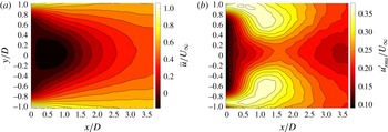
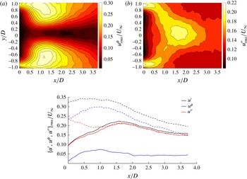
. The spanwise-averaged (the flow may be considered as infinite in the spanwise direction since we are at the centre of the cylinder) mean,
$x=0$
. The spanwise-averaged (the flow may be considered as infinite in the spanwise direction since we are at the centre of the cylinder) mean,
 $\overline{u}$
, and root-mean-square (r.m.s.),
$\overline{u}$
, and root-mean-square (r.m.s.),
 $u_{rms}^{\prime }$
(i.e. before the triple decomposition of (1.5) is applied), streamwise velocity fields are presented in figure 1.
$u_{rms}^{\prime }$
(i.e. before the triple decomposition of (1.5) is applied), streamwise velocity fields are presented in figure 1.
Spanwise-averaged mean,
 $\overline{u}$
, (a) and r.m.s.,
$\overline{u}$
, (a) and r.m.s.,
 $u_{rms}^{\prime }$
, (b) of the streamwise component of the velocity within the experimental field of view.
$u_{rms}^{\prime }$
, (b) of the streamwise component of the velocity within the experimental field of view.
In order to capture the three-dimensional three-component (3D3C) data that were required to compute the statistics of the velocity-gradient tensor tomographic PIV experiments were conducted that imaged the flow immediately downstream of the cylinder in a field of view (FOV) that measured
 $3.8D\times 2D\times 0.168D$
. The flume was homogeneously seeded with polyamide particles of diameter
$3.8D\times 2D\times 0.168D$
. The flume was homogeneously seeded with polyamide particles of diameter
 $56~\unicode[STIX]{x03BC}\text{m}$
which comfortably met the requirement to act as tracers and the FOV was illuminated with the frequency doubled output of a dual cavity/double pulsed Nd:YAG laser (
$56~\unicode[STIX]{x03BC}\text{m}$
which comfortably met the requirement to act as tracers and the FOV was illuminated with the frequency doubled output of a dual cavity/double pulsed Nd:YAG laser (
 $200~\text{mJ}~\text{pulse}^{-1}$
output) that was passed through appropriate light cone-forming optics. A variable aperture slit was used to clip the light cone to produce a thickened light sheet (
$200~\text{mJ}~\text{pulse}^{-1}$
output) that was passed through appropriate light cone-forming optics. A variable aperture slit was used to clip the light cone to produce a thickened light sheet (
 ${\approx}7$
mm thick) with a steep illumination gradient at the edges. The FOV was imaged with four cameras (LaVision Imager Pro X) with
${\approx}7$
mm thick) with a steep illumination gradient at the edges. The FOV was imaged with four cameras (LaVision Imager Pro X) with
 $2048\times 2048$
pixel charge-coupled device sensors with 14 bit grey-scale dynamic range, mounted to Scheimpflug adapters and lenses (Nikkor) with a focal length of
$2048\times 2048$
pixel charge-coupled device sensors with 14 bit grey-scale dynamic range, mounted to Scheimpflug adapters and lenses (Nikkor) with a focal length of
 $f=105$
mm. The off-axis viewing angles were deliberately kept small, as were the apertures of the lenses (
$f=105$
mm. The off-axis viewing angles were deliberately kept small, as were the apertures of the lenses (
 $f/16$
), such that water prisms were not deemed necessary due to the changes in refractive index at the tunnel wall.
$f/16$
), such that water prisms were not deemed necessary due to the changes in refractive index at the tunnel wall.
 $N=2000$
(
$N=2000$
(
 $\times 4$
cameras) image pairs were captured at an acquisition frequency of 0.76 Hz with an inter-frame time of
$\times 4$
cameras) image pairs were captured at an acquisition frequency of 0.76 Hz with an inter-frame time of
 $\unicode[STIX]{x1D6FF}t=1$
ms. A convergence study showed that this was a sufficient number of images to converge the computation of the mean fluctuating components of velocity to zero. These images were processed using the multiplicative algebraic reconstruction technique (MART) tomographic PIV algorithm to produce the tomographic volume reconstruction (Elsinga et al.
Reference Elsinga, Scarano, Wieneke and van Oudheusden2006). To improve the quality of this reconstruction the images were pre-processed with a background subtraction (from previously acquired dark images) and Gaussian smoothing using a
$\unicode[STIX]{x1D6FF}t=1$
ms. A convergence study showed that this was a sufficient number of images to converge the computation of the mean fluctuating components of velocity to zero. These images were processed using the multiplicative algebraic reconstruction technique (MART) tomographic PIV algorithm to produce the tomographic volume reconstruction (Elsinga et al.
Reference Elsinga, Scarano, Wieneke and van Oudheusden2006). To improve the quality of this reconstruction the images were pre-processed with a background subtraction (from previously acquired dark images) and Gaussian smoothing using a
 $3\times 3$
pixel filter length and volume self-calibration (Wieneke Reference Wieneke2008) was applied. The particle displacement field was obtained from these reconstructed volumes using an iterative cross-correlation technique. The final volume size was
$3\times 3$
pixel filter length and volume self-calibration (Wieneke Reference Wieneke2008) was applied. The particle displacement field was obtained from these reconstructed volumes using an iterative cross-correlation technique. The final volume size was
 $32\times 32\times 32$
voxels and an overlap of 75 % between adjacent correlation volumes was used. This translates to a spatial resolution of
$32\times 32\times 32$
voxels and an overlap of 75 % between adjacent correlation volumes was used. This translates to a spatial resolution of
 $0.0486D$
, with a vector spacing of
$0.0486D$
, with a vector spacing of
 $0.0122D$
. This spatial resolution equates to approximately
$0.0122D$
. This spatial resolution equates to approximately
 $11\unicode[STIX]{x1D702}$
, where
$11\unicode[STIX]{x1D702}$
, where
 $\unicode[STIX]{x1D702}$
is the Kolmogorov length scale, for
$\unicode[STIX]{x1D702}$
is the Kolmogorov length scale, for
 $x/D\gtrsim 1.5$
up to a worst case scenario of
$x/D\gtrsim 1.5$
up to a worst case scenario of
 ${\approx}17\unicode[STIX]{x1D702}$
in the separated shear layers at
${\approx}17\unicode[STIX]{x1D702}$
in the separated shear layers at
 $x/D=0$
. Whilst a spatial resolution of
$x/D=0$
. Whilst a spatial resolution of
 ${\approx}3\unicode[STIX]{x1D702}$
is generally considered necessary to resolve the smallest, dissipative length scales within a turbulent flow (Worth, Nickels & Swaminathan Reference Worth, Nickels and Swaminathan2010; Buxton, Laizet & Ganapathisubramani Reference Buxton, Laizet and Ganapathisubramani2011) it has been shown that resolving the characteristic ‘tear drop’ shape of the joint p.d.f. between
${\approx}3\unicode[STIX]{x1D702}$
is generally considered necessary to resolve the smallest, dissipative length scales within a turbulent flow (Worth, Nickels & Swaminathan Reference Worth, Nickels and Swaminathan2010; Buxton, Laizet & Ganapathisubramani Reference Buxton, Laizet and Ganapathisubramani2011) it has been shown that resolving the characteristic ‘tear drop’ shape of the joint p.d.f. between
 $Q$
and
$Q$
and
 $R$
is reliant upon a mix of dissipative and inertial range scales
$R$
is reliant upon a mix of dissipative and inertial range scales
 ${>}\unicode[STIX]{x1D706}$
, where
${>}\unicode[STIX]{x1D706}$
, where
 $\unicode[STIX]{x1D706}$
is the Taylor micro-scale (Buxton Reference Buxton2015). The spatial resolution of the present data easily meet this criteria (it is no worse than
$\unicode[STIX]{x1D706}$
is the Taylor micro-scale (Buxton Reference Buxton2015). The spatial resolution of the present data easily meet this criteria (it is no worse than
 $0.4\unicode[STIX]{x1D706}$
and remains better than
$0.4\unicode[STIX]{x1D706}$
and remains better than
 $0.15\unicode[STIX]{x1D706}$
everywhere other than within the mean recirculation region) and thus this data set may be considered adequately spatially resolved to examine the statistics of the velocity-gradient tensor invariants.
$0.15\unicode[STIX]{x1D706}$
everywhere other than within the mean recirculation region) and thus this data set may be considered adequately spatially resolved to examine the statistics of the velocity-gradient tensor invariants.
2.2 Numerical differentiation and data post-processing
A fourth-order accurate in space, centred finite-difference scheme was used to compute the nine components of the VGT. Only the central five planes of the velocity field were retained due to deteriorating signal-to-noise ratio for the cross-correlations obtained in the volumetric PIV processing towards the edge of the thickened light sheet. Nevertheless, this was satisfactory for the implementation of the fourth-order accurate central-differencing scheme, with only the central plane being retained for the VGT field. By necessity, a lower-order accurate numerical scheme would have been required to compute the spatial velocity gradients in the outer planes, hence they were discarded. An excellent test of the quality of a 3D3C data set from which the velocity gradients are computed is the scatter on the divergence of the velocity field. For an incompressible flow
 $\unicode[STIX]{x2202}u_{i}/\unicode[STIX]{x2202}x_{i}=0$
. However, the presence of experimental noise on a data set leads to spurious, non-zero divergence.
$\unicode[STIX]{x2202}u_{i}/\unicode[STIX]{x2202}x_{i}=0$
. However, the presence of experimental noise on a data set leads to spurious, non-zero divergence.
In order to correct for this non-zero divergence the data were post-processed using the divergence correction scheme of de Silva, Philip & Marusic (Reference de Silva, Philip and Marusic2013). This consists of a nonlinear constraint based optimisation that minimally alters the measured velocity field under the constraint of restricting the magnitude of the divergence to a specified level. The tolerable divergence error was specified as
 $|\unicode[STIX]{x2202}\tilde{u} _{i}/\unicode[STIX]{x2202}x_{i}|\leqslant 1~\text{s}^{-1}$
, in which
$|\unicode[STIX]{x2202}\tilde{u} _{i}/\unicode[STIX]{x2202}x_{i}|\leqslant 1~\text{s}^{-1}$
, in which
 $\tilde{\cdot }$
denotes the application of the divergence correction scheme. The objective function that is minimised during the optimisation is effectively the ensemble average of the ‘turbulent kinetic energy’ that is added to the experimentally measured velocity field, i.e.
$\tilde{\cdot }$
denotes the application of the divergence correction scheme. The objective function that is minimised during the optimisation is effectively the ensemble average of the ‘turbulent kinetic energy’ that is added to the experimentally measured velocity field, i.e.
 $\tilde{k}=\sum _{i=1}^{3}\langle (\tilde{u} _{i}-u_{i})^{2}\rangle$
, which was computed to be
$\tilde{k}=\sum _{i=1}^{3}\langle (\tilde{u} _{i}-u_{i})^{2}\rangle$
, which was computed to be
 $\tilde{k}^{1/2}/U_{\infty }=0.029$
, which is comparable to the experimental error as estimated by the method of Herpin et al. (Reference Herpin, Wong, Stanislas and Soria2008). The extent of the divergence of the final, corrected velocity field is presented in figure 2 which shows the joint p.d.f. between
$\tilde{k}^{1/2}/U_{\infty }=0.029$
, which is comparable to the experimental error as estimated by the method of Herpin et al. (Reference Herpin, Wong, Stanislas and Soria2008). The extent of the divergence of the final, corrected velocity field is presented in figure 2 which shows the joint p.d.f. between
 $\unicode[STIX]{x2202}\tilde{u} /\unicode[STIX]{x2202}x$
and
$\unicode[STIX]{x2202}\tilde{u} /\unicode[STIX]{x2202}x$
and
 $-(\unicode[STIX]{x2202}\tilde{v}/\unicode[STIX]{x2202}y+\unicode[STIX]{x2202}\tilde{w}/\unicode[STIX]{x2202}z)$
. Henceforth, for convenience, all velocity fields will be computed from the divergence corrected data and thus the
$-(\unicode[STIX]{x2202}\tilde{v}/\unicode[STIX]{x2202}y+\unicode[STIX]{x2202}\tilde{w}/\unicode[STIX]{x2202}z)$
. Henceforth, for convenience, all velocity fields will be computed from the divergence corrected data and thus the
 $\tilde{\cdot }$
notation is dropped.
$\tilde{\cdot }$
notation is dropped.
Joint p.d.f. between
 $\unicode[STIX]{x2202}\tilde{u} /\unicode[STIX]{x2202}x$
and
$\unicode[STIX]{x2202}\tilde{u} /\unicode[STIX]{x2202}x$
and
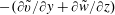 $-(\unicode[STIX]{x2202}\tilde{v}/\unicode[STIX]{x2202}y+\unicode[STIX]{x2202}\tilde{w}/\unicode[STIX]{x2202}z)$
, where
$-(\unicode[STIX]{x2202}\tilde{v}/\unicode[STIX]{x2202}y+\unicode[STIX]{x2202}\tilde{w}/\unicode[STIX]{x2202}z)$
, where
 $\tilde{\cdot }$
denotes the application of the divergence correction scheme of (de Silva et al.
Reference de Silva, Philip and Marusic2013) to the data.
$\tilde{\cdot }$
denotes the application of the divergence correction scheme of (de Silva et al.
Reference de Silva, Philip and Marusic2013) to the data.
3 Phase averaging and the triple decomposition
Since the data were acquired at a rate that is significantly slower than the characteristic shedding frequency of the cylinder it is necessary to compute the coherent velocity fluctuations,
 $u_{i}^{\unicode[STIX]{x1D719}}$
in (1.5), by computing/approximating a phase average. Whilst Baj et al. (Reference Baj, Bruce and Buxton2015) shows that this is inadequate for a multi-scale flow it has proven to be satisfactory for a single cylinder flow (Cantwell & Coles Reference Cantwell and Coles1983). The determination of the phase of the instantaneous velocity fields was achieved through the use of proper orthogonal decomposition (POD) (Berkooz, Holmes & Lumley Reference Berkooz, Holmes and Lumley1993). POD is a linear procedure for extracting a basis for modal decomposition of an ensemble of velocity fields, such as that acquired during the tomographic PIV experiments. These modes,
$u_{i}^{\unicode[STIX]{x1D719}}$
in (1.5), by computing/approximating a phase average. Whilst Baj et al. (Reference Baj, Bruce and Buxton2015) shows that this is inadequate for a multi-scale flow it has proven to be satisfactory for a single cylinder flow (Cantwell & Coles Reference Cantwell and Coles1983). The determination of the phase of the instantaneous velocity fields was achieved through the use of proper orthogonal decomposition (POD) (Berkooz, Holmes & Lumley Reference Berkooz, Holmes and Lumley1993). POD is a linear procedure for extracting a basis for modal decomposition of an ensemble of velocity fields, such as that acquired during the tomographic PIV experiments. These modes,
 $\unicode[STIX]{x1D6F9}_{j}$
where
$\unicode[STIX]{x1D6F9}_{j}$
where
 $1\leqslant j\leqslant N$
, are ranked according to their kinetic energy content. The first mode is steady, and corresponds to the base (or time-averaged mean) flow. van Oudheusden et al. (Reference van Oudheusden, Scarano, van Hinsberg and Watt2005) showed that the next two most energetic modes correspond to the vortex shedding of the cylinder and that a low-order model of the flow consisting of the base flow,
$1\leqslant j\leqslant N$
, are ranked according to their kinetic energy content. The first mode is steady, and corresponds to the base (or time-averaged mean) flow. van Oudheusden et al. (Reference van Oudheusden, Scarano, van Hinsberg and Watt2005) showed that the next two most energetic modes correspond to the vortex shedding of the cylinder and that a low-order model of the flow consisting of the base flow,
 $\unicode[STIX]{x1D6F9}_{2}$
and
$\unicode[STIX]{x1D6F9}_{2}$
and
 $\unicode[STIX]{x1D6F9}_{3}$
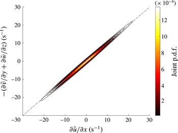
is practically equivalent to the phase-averaged result. Figure 3 shows the proportion of total kinetic energy in the first 10 modes. It can be seen that after the base flow, mode 1, the majority of the energy is contained within modes 2 and 3 as is expected in the flow downstream of a cylinder (Perrin et al.
Reference Perrin, Braza, Cid, Cazin, Barthet, Sevrain, Mockett and Thiele2007).
$\unicode[STIX]{x1D6F9}_{3}$
is practically equivalent to the phase-averaged result. Figure 3 shows the proportion of total kinetic energy in the first 10 modes. It can be seen that after the base flow, mode 1, the majority of the energy is contained within modes 2 and 3 as is expected in the flow downstream of a cylinder (Perrin et al.
Reference Perrin, Braza, Cid, Cazin, Barthet, Sevrain, Mockett and Thiele2007).
Proportion of total kinetic energy content within the first 10 POD modes.
Despite the fidelity of a lower-order model consisting of the base flow (
 $\overline{\boldsymbol{u}}$
) and modes
$\overline{\boldsymbol{u}}$
) and modes
 $\unicode[STIX]{x1D6F9}_{2}$
and
$\unicode[STIX]{x1D6F9}_{2}$
and
 $\unicode[STIX]{x1D6F9}_{3}$
we choose to use a phase bin-averaging procedure similar to the approach taken by Perrin et al. (Reference Perrin, Braza, Cid, Cazin, Chassaing, Mockett, Reimann and Thiele2008), which is shown to more faithfully reproduce the coherent motions. Each POD mode,
$\unicode[STIX]{x1D6F9}_{3}$
we choose to use a phase bin-averaging procedure similar to the approach taken by Perrin et al. (Reference Perrin, Braza, Cid, Cazin, Chassaing, Mockett, Reimann and Thiele2008), which is shown to more faithfully reproduce the coherent motions. Each POD mode,
 $\unicode[STIX]{x1D6F9}_{j}$
, has a corresponding time varying mode coefficient
$\unicode[STIX]{x1D6F9}_{j}$
, has a corresponding time varying mode coefficient
 $a_{j}$
. Since modes
$a_{j}$
. Since modes
 $\unicode[STIX]{x1D6F9}_{2}$
and
$\unicode[STIX]{x1D6F9}_{2}$
and
 $\unicode[STIX]{x1D6F9}_{3}$
are orthogonal to one another a phase angle may be defined from the
$\unicode[STIX]{x1D6F9}_{3}$
are orthogonal to one another a phase angle may be defined from the
 $a_{2}{-}a_{3}$
plane. The scatter plot of
$a_{2}{-}a_{3}$
plane. The scatter plot of
 $a_{2}/\sqrt{2\unicode[STIX]{x1D709}_{2}}$
versus
$a_{2}/\sqrt{2\unicode[STIX]{x1D709}_{2}}$
versus
 $a_{3}/\sqrt{2\unicode[STIX]{x1D709}_{3}}$
, in which
$a_{3}/\sqrt{2\unicode[STIX]{x1D709}_{3}}$
, in which
 $\unicode[STIX]{x1D709}_{j}$
is the corresponding eigenvalue to
$\unicode[STIX]{x1D709}_{j}$
is the corresponding eigenvalue to
 $\unicode[STIX]{x1D6F9}_{j}$
(not shown for brevity), shows a pattern scattered around a unit circle with its centre at the origin as expected (van Oudheusden et al.
Reference van Oudheusden, Scarano, van Hinsberg and Watt2005). Each instantaneous velocity field is then assigned a phase angle such that
$\unicode[STIX]{x1D6F9}_{j}$
(not shown for brevity), shows a pattern scattered around a unit circle with its centre at the origin as expected (van Oudheusden et al.
Reference van Oudheusden, Scarano, van Hinsberg and Watt2005). Each instantaneous velocity field is then assigned a phase angle such that
 $$\begin{eqnarray}\tan \unicode[STIX]{x1D719}=\frac{a_{3}}{a_{2}}\sqrt{\frac{\unicode[STIX]{x1D709}_{2}}{\unicode[STIX]{x1D709}_{3}}}.\end{eqnarray}$$
The phase space is discretised into 18 phase bins centred on
 $\unicode[STIX]{x1D719}_{0m}$
(
$\unicode[STIX]{x1D719}_{0m}$
(
 $1\leqslant m\leqslant 18$
) of size
$1\leqslant m\leqslant 18$
) of size
 $\unicode[STIX]{x0394}\unicode[STIX]{x1D719}=20^{\circ }$
. All velocity fields for which the phase angle
$\unicode[STIX]{x0394}\unicode[STIX]{x1D719}=20^{\circ }$
. All velocity fields for which the phase angle
 $\unicode[STIX]{x1D719}\in (\unicode[STIX]{x1D719}_{0m}\pm \unicode[STIX]{x0394}\unicode[STIX]{x1D719}/2)$
were ensemble averaged in order to compute
$\unicode[STIX]{x1D719}\in (\unicode[STIX]{x1D719}_{0m}\pm \unicode[STIX]{x0394}\unicode[STIX]{x1D719}/2)$
were ensemble averaged in order to compute
 $u_{i}^{\unicode[STIX]{x1D719}}$
and subsequently
$u_{i}^{\unicode[STIX]{x1D719}}$
and subsequently
 $u_{i}^{\prime \prime }$
as below
$u_{i}^{\prime \prime }$
as below
 $$\begin{eqnarray}\displaystyle & \displaystyle u_{i}^{\unicode[STIX]{x1D719}}(m)=\langle U_{i}(\unicode[STIX]{x1D719})-\overline{u}_{i}\rangle \quad \forall \;(\unicode[STIX]{x1D719}_{0m}-\unicode[STIX]{x0394}\unicode[STIX]{x1D719}/2\leqslant \unicode[STIX]{x1D719}\leqslant \unicode[STIX]{x1D719}_{0m}+\unicode[STIX]{x0394}\unicode[STIX]{x1D719}/2) & \displaystyle\end{eqnarray}$$
 $$\begin{eqnarray}\displaystyle & \displaystyle u_{i}^{\prime \prime }=U_{i}-\overline{u}_{i}-u_{i}^{\unicode[STIX]{x1D719}}(m). & \displaystyle\end{eqnarray}$$
Note that the variable
 $u_{i}^{\unicode[STIX]{x1D719}}(m)$
is discrete since the phase averaging is conducted over bins of size
$u_{i}^{\unicode[STIX]{x1D719}}(m)$
is discrete since the phase averaging is conducted over bins of size
 $\unicode[STIX]{x0394}\unicode[STIX]{x1D719}=20^{\circ }$
, however for convenience this discrete notation is dropped for the remainder of the manuscript and the coherent velocity fluctuation is henceforth simply referred to as
$\unicode[STIX]{x0394}\unicode[STIX]{x1D719}=20^{\circ }$
, however for convenience this discrete notation is dropped for the remainder of the manuscript and the coherent velocity fluctuation is henceforth simply referred to as
 $u_{i}^{\unicode[STIX]{x1D719}}$
. The r.m.s. fields of both
$u_{i}^{\unicode[STIX]{x1D719}}$
. The r.m.s. fields of both
 $u^{\unicode[STIX]{x1D719}}$
and
$u^{\unicode[STIX]{x1D719}}$
and
 $u^{\prime \prime }$
are presented in figure 4.
$u^{\prime \prime }$
are presented in figure 4.
Both the
 $\boldsymbol{u}^{\unicode[STIX]{x1D719}}(\boldsymbol{x})$
and
$\boldsymbol{u}^{\unicode[STIX]{x1D719}}(\boldsymbol{x})$
and
 $\boldsymbol{u}^{\prime \prime }(\boldsymbol{x})$
fields were numerically differentiated with the same fourth-order accurate scheme as described in § 2.2 and the divergence of both was computed. Whilst the scatter for both
$\boldsymbol{u}^{\prime \prime }(\boldsymbol{x})$
fields were numerically differentiated with the same fourth-order accurate scheme as described in § 2.2 and the divergence of both was computed. Whilst the scatter for both
 $\unicode[STIX]{x2202}u_{i}^{\unicode[STIX]{x1D719}}/\unicode[STIX]{x2202}x_{i}$
and
$\unicode[STIX]{x2202}u_{i}^{\unicode[STIX]{x1D719}}/\unicode[STIX]{x2202}x_{i}$
and
 $\unicode[STIX]{x2202}u_{i}^{\prime \prime }/\unicode[STIX]{x2202}x_{i}$
was higher than for
$\unicode[STIX]{x2202}u_{i}^{\prime \prime }/\unicode[STIX]{x2202}x_{i}$
was higher than for
 $\unicode[STIX]{x2202}u_{i}^{\prime }/\unicode[STIX]{x2202}x_{i}$
(illustrated in figure 2) both were more than acceptable in comparison to previously published data (e.g. Ganapathisubramani, Lakshminarasimhan & Clemens Reference Ganapathisubramani, Lakshminarasimhan and Clemens2007).
$\unicode[STIX]{x2202}u_{i}^{\prime }/\unicode[STIX]{x2202}x_{i}$
(illustrated in figure 2) both were more than acceptable in comparison to previously published data (e.g. Ganapathisubramani, Lakshminarasimhan & Clemens Reference Ganapathisubramani, Lakshminarasimhan and Clemens2007).
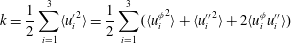
The r.m.s. fields of the coherent (a) and stochastic (b) component of the streamwise velocity fluctuation. (c) Streamwise profiles of r.m.s. of
 $\{u^{\prime },u^{\unicode[STIX]{x1D719}},u^{\prime \prime }\}$
along the centreline (solid lines) and along the shear layers (dashed lines), defined as the locations,
$\{u^{\prime },u^{\unicode[STIX]{x1D719}},u^{\prime \prime }\}$
along the centreline (solid lines) and along the shear layers (dashed lines), defined as the locations,
 $y(x)$
, at which the r.m.s. is locally a maximum.
$y(x)$
, at which the r.m.s. is locally a maximum.
The ensemble-averaged turbulent kinetic energy is given by
 $$\begin{eqnarray}k=\frac{1}{2}\mathop{\sum }_{i=1}^{3}\langle {u_{i}^{\prime }}^{2}\rangle =\frac{1}{2}\mathop{\sum }_{i=1}^{3}(\langle {u_{i}^{\unicode[STIX]{x1D719}}}^{2}\rangle +\langle {u_{i}^{\prime \prime }}^{2}\rangle +2\langle u_{i}^{\unicode[STIX]{x1D719}}u_{i}^{\prime \prime }\rangle )\end{eqnarray}$$
and thus for the triple decomposition to be energy preserving, such that the total turbulent kinetic energy is equal to the sum of that of the coherent and stochastic velocity fluctuation fields, the correlation
 $\langle u_{i}^{\unicode[STIX]{x1D719}}u_{i}^{\prime \prime }\rangle$
must be zero. Within the field of view
$\langle u_{i}^{\unicode[STIX]{x1D719}}u_{i}^{\prime \prime }\rangle$
must be zero. Within the field of view
 $\langle u_{i}^{\unicode[STIX]{x1D719}}u_{i}^{\prime \prime }\rangle /{U_{\infty }}^{2}$
was computed to be
$\langle u_{i}^{\unicode[STIX]{x1D719}}u_{i}^{\prime \prime }\rangle /{U_{\infty }}^{2}$
was computed to be
 $1.4\times 10^{-4}$
, which is zero to within the experimental uncertainty. Nevertheless, this small positive value is a potential explanation for the slightly less strictly observed divergence-free condition in the
$1.4\times 10^{-4}$
, which is zero to within the experimental uncertainty. Nevertheless, this small positive value is a potential explanation for the slightly less strictly observed divergence-free condition in the
 $\boldsymbol{u}^{\unicode[STIX]{x1D719}}(\boldsymbol{x})$
and
$\boldsymbol{u}^{\unicode[STIX]{x1D719}}(\boldsymbol{x})$
and
 $\boldsymbol{u}^{\prime \prime }(\boldsymbol{x})$
fields, since differentiation is known to amplify any noise present.
$\boldsymbol{u}^{\prime \prime }(\boldsymbol{x})$
fields, since differentiation is known to amplify any noise present.
4 Results and discussion
The various fluctuating velocity fields,
 $\boldsymbol{u}^{\prime }(\boldsymbol{x})$
,
$\boldsymbol{u}^{\prime }(\boldsymbol{x})$
,
 $\boldsymbol{u}^{\unicode[STIX]{x1D719}}(\boldsymbol{x})$
and
$\boldsymbol{u}^{\unicode[STIX]{x1D719}}(\boldsymbol{x})$
and
 $\boldsymbol{u}^{\prime \prime }(\boldsymbol{x})$
were differentiated spatially according to the fourth-order accurate scheme described in § 2.2 and the various invariants of the velocity-gradient tensor were computed. The spatial evolution of the joint p.d.f.s of these invariants was computed along two streamwise traverses, the centreline of the flow (
$\boldsymbol{u}^{\prime \prime }(\boldsymbol{x})$
were differentiated spatially according to the fourth-order accurate scheme described in § 2.2 and the various invariants of the velocity-gradient tensor were computed. The spatial evolution of the joint p.d.f.s of these invariants was computed along two streamwise traverses, the centreline of the flow (
 $y=0$
) and along the shear layers. At a given
$y=0$
) and along the shear layers. At a given
 $x$
location the
$x$
location the
 $y$
profiles of the r.m.s. of
$y$
profiles of the r.m.s. of
 $u^{\prime }$
have two local maxima, as indicated in figure 1(b), and thus the shear layers were defined as the locations,
$u^{\prime }$
have two local maxima, as indicated in figure 1(b), and thus the shear layers were defined as the locations,
 $y(x)$
, of these maxima. Due to symmetry it was possible to produce statistics that were averaged over both shear layers to aid with convergence. However, due to the typically observed intermittent distribution of the velocity gradients some spatial averaging was performed, in which a square window of size
$y(x)$
, of these maxima. Due to symmetry it was possible to produce statistics that were averaged over both shear layers to aid with convergence. However, due to the typically observed intermittent distribution of the velocity gradients some spatial averaging was performed, in which a square window of size
 $0.13D\times 0.13D$
was centred on the point of interest (i.e. on the centreline or the shear layer) in order to better converge the statistics. A sensitivity study was conducted to assess the size of this window on the ability to faithfully reproduce the
$0.13D\times 0.13D$
was centred on the point of interest (i.e. on the centreline or the shear layer) in order to better converge the statistics. A sensitivity study was conducted to assess the size of this window on the ability to faithfully reproduce the
 $Q{-}R$
joint p.d.f. and it was found to be optimal in the sense that it was the minimal window size that generated relatively noise-free statistics that were insensitive to modest increases/decreases in window size.
$Q{-}R$
joint p.d.f. and it was found to be optimal in the sense that it was the minimal window size that generated relatively noise-free statistics that were insensitive to modest increases/decreases in window size.
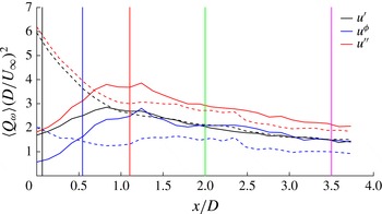
Streamwise profile of
 $\langle Q_{\unicode[STIX]{x1D714}}\rangle$
along the centreline (solid lines) and along the shear layers (dashed lines). The vertical lines indicate the streamwise locations for the joint p.d.f.s of figure 6.
$\langle Q_{\unicode[STIX]{x1D714}}\rangle$
along the centreline (solid lines) and along the shear layers (dashed lines). The vertical lines indicate the streamwise locations for the joint p.d.f.s of figure 6.
Joint p.d.f.s were then produced of the various
 $Q{-}R$
invariants, computed from the
$Q{-}R$
invariants, computed from the
 $\{\unicode[STIX]{x1D622}_{ij},\unicode[STIX]{x1D622}_{ij}^{\unicode[STIX]{x1D719}},\unicode[STIX]{x1D622}_{ij}^{\prime \prime }\}$
fields, at the streamwise locations indicated by the coloured vertical lines of figure 5. In order to make a direct comparison between the joint p.d.f.s computed from the various fields of velocity gradients we wished to choose a contour level that encompasses an equivalent proportion of the overall data available, i.e.
$\{\unicode[STIX]{x1D622}_{ij},\unicode[STIX]{x1D622}_{ij}^{\unicode[STIX]{x1D719}},\unicode[STIX]{x1D622}_{ij}^{\prime \prime }\}$
fields, at the streamwise locations indicated by the coloured vertical lines of figure 5. In order to make a direct comparison between the joint p.d.f.s computed from the various fields of velocity gradients we wished to choose a contour level that encompasses an equivalent proportion of the overall data available, i.e.
 $$\begin{eqnarray}\iint _{A}f_{QR}(Q,R)\,\text{d}R\,\text{d}Q=\unicode[STIX]{x1D6F4}=\text{const.}\end{eqnarray}$$
The choice of
 $\unicode[STIX]{x1D6F4}$
is arbitrary, but we wished to choose a contour level defining
$\unicode[STIX]{x1D6F4}$
is arbitrary, but we wished to choose a contour level defining
 $A$
that was sufficiently rare to ensure that we captured a broad range of
$A$
that was sufficiently rare to ensure that we captured a broad range of
 $Q{-}R$
states but sufficiently common to ensure a reasonably smooth contour from sufficiently converged statistics. We chose a contour level of
$Q{-}R$
states but sufficiently common to ensure a reasonably smooth contour from sufficiently converged statistics. We chose a contour level of
 $\unicode[STIX]{x1D6F4}=0.683$
, which is equivalent to the proportion of data bounded by
$\unicode[STIX]{x1D6F4}=0.683$
, which is equivalent to the proportion of data bounded by
 $\pm \unicode[STIX]{x1D70E}$
(one standard deviation) for a univariate Gaussian distribution. The invariants themselves are all normalised by the local value of
$\pm \unicode[STIX]{x1D70E}$
(one standard deviation) for a univariate Gaussian distribution. The invariants themselves are all normalised by the local value of
 $\langle Q_{\unicode[STIX]{x1D714}}\rangle$
, computed from the relevant velocity-gradient field such that the joint p.d.f.s of figure 6(c), for example, are normalised by
$\langle Q_{\unicode[STIX]{x1D714}}\rangle$
, computed from the relevant velocity-gradient field such that the joint p.d.f.s of figure 6(c), for example, are normalised by
 $\langle Q_{\unicode[STIX]{x1D714}}\rangle$
calculated from the
$\langle Q_{\unicode[STIX]{x1D714}}\rangle$
calculated from the
 $\unicode[STIX]{x1D622}_{ij}^{\unicode[STIX]{x1D719}}$
field at the centreline and appropriate
$\unicode[STIX]{x1D622}_{ij}^{\unicode[STIX]{x1D719}}$
field at the centreline and appropriate
 $x$
-location etc. as illustrated in figure 5.
$x$
-location etc. as illustrated in figure 5.
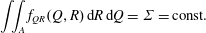
Joint p.d.f.s between
 $Q$
and
$Q$
and
 $R$
along the centreline (a,c,e) and the shear layer (b,d,f) for the
$R$
along the centreline (a,c,e) and the shear layer (b,d,f) for the
 $\unicode[STIX]{x1D622}_{ij}$
(a,b),
$\unicode[STIX]{x1D622}_{ij}$
(a,b),
 $\unicode[STIX]{x1D622}_{ij}^{\unicode[STIX]{x1D719}}$
(c,d) and
$\unicode[STIX]{x1D622}_{ij}^{\unicode[STIX]{x1D719}}$
(c,d) and
 $\unicode[STIX]{x1D622}_{ij}^{\prime \prime }$
(e,f) velocity-gradient fields. The contour colours correspond to the streamwise locations depicted in figure 5.
$\unicode[STIX]{x1D622}_{ij}^{\prime \prime }$
(e,f) velocity-gradient fields. The contour colours correspond to the streamwise locations depicted in figure 5.
It can be seen that the classical ‘tear drop’ shape for the joint p.d.f. is recovered when calculated from the
 $\unicode[STIX]{x1D622}_{ij}$
field. This in itself is a surprising result since the ‘tear drop’ shape of the
$\unicode[STIX]{x1D622}_{ij}$
field. This in itself is a surprising result since the ‘tear drop’ shape of the
 $Q{-}R$
joint p.d.f. is considered to be associated with fully developed turbulent flows. Although there is no clear definition of such a flow they may be generally considered to be close to homogeneous and isotropic (requiring the integral length scale to be smaller than a relevant homogeneity length scale), in the small scales at least, with mean velocity profiles that may be collapsed when scaled by a relevant flow variable such as the centreline velocity for a wake. Evidently these criteria are far from being met in the near-field flow behind a square cylinder. It is clear from inspection of figure 1 that throughout the field of view, but particularly for the cases of
$Q{-}R$
joint p.d.f. is considered to be associated with fully developed turbulent flows. Although there is no clear definition of such a flow they may be generally considered to be close to homogeneous and isotropic (requiring the integral length scale to be smaller than a relevant homogeneity length scale), in the small scales at least, with mean velocity profiles that may be collapsed when scaled by a relevant flow variable such as the centreline velocity for a wake. Evidently these criteria are far from being met in the near-field flow behind a square cylinder. It is clear from inspection of figure 1 that throughout the field of view, but particularly for the cases of
 $x/D\leqslant 2$
, the flow is far from homogeneous. Further, the ‘tear drop’-shaped contours are equally visible, and quantitatively similar (with the exception of the
$x/D\leqslant 2$
, the flow is far from homogeneous. Further, the ‘tear drop’-shaped contours are equally visible, and quantitatively similar (with the exception of the
 $x/D=3.5$
cases) on both the centreline and the shear layers in figure 6(a,b). This is despite the fact that the flow physics for both of these regions differ significantly. Figure 1 shows that along the centreline the shape of the
$x/D=3.5$
cases) on both the centreline and the shear layers in figure 6(a,b). This is despite the fact that the flow physics for both of these regions differ significantly. Figure 1 shows that along the centreline the shape of the
 $Q{-}R$
joint p.d.f. contours are similar regardless of whether the data are extracted from the mean circulation region (for the centreline) or downstream of this in the turbulence decay region (
$Q{-}R$
joint p.d.f. contours are similar regardless of whether the data are extracted from the mean circulation region (for the centreline) or downstream of this in the turbulence decay region (
 $x/D=2$
). Perversely,
$x/D=2$
). Perversely,
 $x/D=3.5$
is perhaps the location where one might assume that the criteria for a fully developed turbulent flow, for which the ‘tear drop’-shaped joint p.d.f. is considered to be a universal feature, are more stringently met than any of the streamwise locations further upstream. Despite this, the joint p.d.f.s from this location are the only ones not to collapse when normalised by
$x/D=3.5$
is perhaps the location where one might assume that the criteria for a fully developed turbulent flow, for which the ‘tear drop’-shaped joint p.d.f. is considered to be a universal feature, are more stringently met than any of the streamwise locations further upstream. Despite this, the joint p.d.f.s from this location are the only ones not to collapse when normalised by
 $\langle Q_{\unicode[STIX]{x1D714}}\rangle$
. The clearly defined ‘tear drop’-shaped contours of the joint p.d.f.s of figure 6(a,b) are in contrast to the spatially developing fractal square grid flow of (Gomes-Fernandes et al.
Reference Gomes-Fernandes, Ganapathisubramani and Vassilicos2014), in which the ‘tear drop’ shape was observed to unfold as the flow develops downstream, in particular the ‘Vieillefosse tail’ and contribution of sector
$\langle Q_{\unicode[STIX]{x1D714}}\rangle$
. The clearly defined ‘tear drop’-shaped contours of the joint p.d.f.s of figure 6(a,b) are in contrast to the spatially developing fractal square grid flow of (Gomes-Fernandes et al.
Reference Gomes-Fernandes, Ganapathisubramani and Vassilicos2014), in which the ‘tear drop’ shape was observed to unfold as the flow develops downstream, in particular the ‘Vieillefosse tail’ and contribution of sector
 $I$
became increasingly significant whereas the contribution of sector
$I$
became increasingly significant whereas the contribution of sector
 $II$
was reduced.
$II$
was reduced.
Comparison of figure 6(a,b) shows that the collapse of the contours of
 $f_{QR}(Q,R)$
when scaled with the local quantity
$f_{QR}(Q,R)$
when scaled with the local quantity
 $\langle Q_{\unicode[STIX]{x1D714}}\rangle$
is marginally better along the shear layer than the centreline, excluding the data from
$\langle Q_{\unicode[STIX]{x1D714}}\rangle$
is marginally better along the shear layer than the centreline, excluding the data from
 $x/D=3.5$
. There is significant energy content in coherent motions in the shear layers, as illustrated in figure 4(a), whereas along the centreline there is virtually none with a significant contribution to the total turbulent kinetic energy from the
$x/D=3.5$
. There is significant energy content in coherent motions in the shear layers, as illustrated in figure 4(a), whereas along the centreline there is virtually none with a significant contribution to the total turbulent kinetic energy from the
 $u_{i}^{\prime \prime }$
fluctuations. It is thus a surprising result that the collapse of the contours of
$u_{i}^{\prime \prime }$
fluctuations. It is thus a surprising result that the collapse of the contours of
 $f_{QR}(Q,R)$
is better where there is a significant contribution from coherent motions as opposed to primarily the stochastic fluctuations. Nevertheless, the similarity between the contours of figure 6(a,b) is stark, despite the fact that they are computed from regions with very different flow physics to one another. The streamwise location at which the joint p.d.f. most resembles that for fully developed turbulence, with an enhanced contribution from sector
$f_{QR}(Q,R)$
is better where there is a significant contribution from coherent motions as opposed to primarily the stochastic fluctuations. Nevertheless, the similarity between the contours of figure 6(a,b) is stark, despite the fact that they are computed from regions with very different flow physics to one another. The streamwise location at which the joint p.d.f. most resembles that for fully developed turbulence, with an enhanced contribution from sector
 $I$
and elongated ‘Vieillefosse tail’ is at the location of peak turbulence intensity,
$I$
and elongated ‘Vieillefosse tail’ is at the location of peak turbulence intensity,
 $x/D=1.104$
.
$x/D=1.104$
.
Figure 6(c,d) shows the equivalent joint p.d.f.s between
 $Q$
and
$Q$
and
 $R$
computed from the coherent velocity-gradient field,
$R$
computed from the coherent velocity-gradient field,
 $\unicode[STIX]{x1D622}_{ij}^{\unicode[STIX]{x1D719}}$
, along the centreline and shear layer, respectively whilst (e) and (f) show those computed from the stochastic velocity-gradient field,
$\unicode[STIX]{x1D622}_{ij}^{\unicode[STIX]{x1D719}}$
, along the centreline and shear layer, respectively whilst (e) and (f) show those computed from the stochastic velocity-gradient field,
 $\unicode[STIX]{x1D622}_{ij}^{\prime \prime }$
. It is clear that the contours of
$\unicode[STIX]{x1D622}_{ij}^{\prime \prime }$
. It is clear that the contours of
 $f_{QR}(Q,R)$
computed from the
$f_{QR}(Q,R)$
computed from the
 $\unicode[STIX]{x1D622}_{ij}^{\unicode[STIX]{x1D719}}$
field do not exhibit anything remotely akin to a ‘tear drop’ shape, whilst those computed from the
$\unicode[STIX]{x1D622}_{ij}^{\unicode[STIX]{x1D719}}$
field do not exhibit anything remotely akin to a ‘tear drop’ shape, whilst those computed from the
 $\unicode[STIX]{x1D622}_{ij}^{\prime \prime }$
field do, and are indeed quantitatively very similar to those computed from the
$\unicode[STIX]{x1D622}_{ij}^{\prime \prime }$
field do, and are indeed quantitatively very similar to those computed from the
 $\unicode[STIX]{x1D622}_{ij}$
field. If anything, it may be commented that the contours show a better collapse with the local
$\unicode[STIX]{x1D622}_{ij}$
field. If anything, it may be commented that the contours show a better collapse with the local
 $\langle Q_{\unicode[STIX]{x1D714}}\rangle$
scaling for the joint p.d.f. computed from the
$\langle Q_{\unicode[STIX]{x1D714}}\rangle$
scaling for the joint p.d.f. computed from the
 $\unicode[STIX]{x1D622}_{ij}^{\prime \prime }$
field than from the
$\unicode[STIX]{x1D622}_{ij}^{\prime \prime }$
field than from the
 $\unicode[STIX]{x1D622}_{ij}$
field. Again, however, the notable exception is the contour extracted from the data at the furthest downstream location,
$\unicode[STIX]{x1D622}_{ij}$
field. Again, however, the notable exception is the contour extracted from the data at the furthest downstream location,
 $x/D=3.5$
, at which we may have expected the flow to best approximate a ‘fully developed flow’.
$x/D=3.5$
, at which we may have expected the flow to best approximate a ‘fully developed flow’.
We may thus conclude from figure 6 that in this spatially developing inhomogeneous flow the ‘tear drop’ shape of the contours of the joint p.d.f. between
 $Q$
and
$Q$
and
 $R$
is almost entirely due to the stochastic turbulent fluctuations. Even though figure 5 shows that the coherent motions have a non-negligible
$R$
is almost entirely due to the stochastic turbulent fluctuations. Even though figure 5 shows that the coherent motions have a non-negligible
 $\langle Q_{\unicode[STIX]{x1D714}}\rangle$
, indicative of the average magnitude of the
$\langle Q_{\unicode[STIX]{x1D714}}\rangle$
, indicative of the average magnitude of the
 $\unicode[STIX]{x1D622}_{ij}^{\unicode[STIX]{x1D719}}$
tensor, it does not contribute to the kinematics of the overall velocity-gradient tensor through the
$\unicode[STIX]{x1D622}_{ij}^{\unicode[STIX]{x1D719}}$
tensor, it does not contribute to the kinematics of the overall velocity-gradient tensor through the
 $Q{-}R$
joint p.d.f. It thus appears that the ‘tear drop’ is more ubiquitous than first thought since it appears in flows with significantly varied physics (fully developed/spatially developing/recirculation/separated shear layers etc.) in an observation that is comparable to the ‘embarrassment of success’ of Kolmogorov’s 1941 theory (Kraichnan Reference Kraichnan1974). Kolmogorov (Reference Kolmogorov1941) predicts the existence of a
$Q{-}R$
joint p.d.f. It thus appears that the ‘tear drop’ is more ubiquitous than first thought since it appears in flows with significantly varied physics (fully developed/spatially developing/recirculation/separated shear layers etc.) in an observation that is comparable to the ‘embarrassment of success’ of Kolmogorov’s 1941 theory (Kraichnan Reference Kraichnan1974). Kolmogorov (Reference Kolmogorov1941) predicts the existence of a
 $-5/3$
slope of the energy spectrum in homogeneous, isotropic turbulence for which the Reynolds number is sufficiently high to support an inertial range of scales separating the dissipative and large-scale motions. Equation (1.4) shows that the invariant
$-5/3$
slope of the energy spectrum in homogeneous, isotropic turbulence for which the Reynolds number is sufficiently high to support an inertial range of scales separating the dissipative and large-scale motions. Equation (1.4) shows that the invariant
 $R$
is the local excess of strain-rate production over enstrophy amplification,
$R$
is the local excess of strain-rate production over enstrophy amplification,
 $\unicode[STIX]{x1D714}_{i}\unicode[STIX]{x1D634}_{ij}\unicode[STIX]{x1D714}_{j}$
. The amplification of enstrophy, through its interaction with the strain-rate field, is the only known inertial mechanism by which enstrophy (and turbulent kinetic energy) are transferred (on average) to smaller scales through the turbulent cascade. Contrastingly, equation (1.3) shows that the invariant
$\unicode[STIX]{x1D714}_{i}\unicode[STIX]{x1D634}_{ij}\unicode[STIX]{x1D714}_{j}$
. The amplification of enstrophy, through its interaction with the strain-rate field, is the only known inertial mechanism by which enstrophy (and turbulent kinetic energy) are transferred (on average) to smaller scales through the turbulent cascade. Contrastingly, equation (1.3) shows that the invariant
 $Q$
is representative of the localised topology of the flow, whether rotationally or strain-rate dominated. Numerous studies (e.g. Ruetsch & Maxey Reference Ruetsch and Maxey1991) have painted a consistent topological picture of developed, fine-scale turbulence in which sheets of dissipation (high magnitude strain rate) are wrapped around ‘worms’ of intense enstrophy. Yet figure 6 clearly shows ‘tear drop’-shaped distributions of
$Q$
is representative of the localised topology of the flow, whether rotationally or strain-rate dominated. Numerous studies (e.g. Ruetsch & Maxey Reference Ruetsch and Maxey1991) have painted a consistent topological picture of developed, fine-scale turbulence in which sheets of dissipation (high magnitude strain rate) are wrapped around ‘worms’ of intense enstrophy. Yet figure 6 clearly shows ‘tear drop’-shaped distributions of
 $Q$
and
$Q$
and
 $R$
in a flow that is highly inhomogeneous/anisotropic with wildly varying flow topologies, mirroring the finding of a
$R$
in a flow that is highly inhomogeneous/anisotropic with wildly varying flow topologies, mirroring the finding of a
 $-5/3$
slope in flows at modest Reynolds numbers that are also far from homogeneous/isotropic (e.g. Valente & Vassilicos Reference Valente and Vassilicos2012; Gomes-Fernandes et al.
Reference Gomes-Fernandes, Ganapathisubramani and Vassilicos2015; Laizet, Nedić & Vassilicos Reference Laizet, Nedić and Vassilicos2015).
$-5/3$
slope in flows at modest Reynolds numbers that are also far from homogeneous/isotropic (e.g. Valente & Vassilicos Reference Valente and Vassilicos2012; Gomes-Fernandes et al.
Reference Gomes-Fernandes, Ganapathisubramani and Vassilicos2015; Laizet, Nedić & Vassilicos Reference Laizet, Nedić and Vassilicos2015).


Figure 6 illustrates contours of the joint p.d.f.s between the invariants
 $Q$
and
$Q$
and
 $R$
at several illustrative downstream locations. However, the nature of the tomographic PIV data that have been acquired allows a closer inspection of the spatial development of the statistical distribution of these invariants. This may be quantified by computing the proportions of the total data located within various sectors of the joint p.d.f. The majority of the total data are locally swirling, i.e.
$R$
at several illustrative downstream locations. However, the nature of the tomographic PIV data that have been acquired allows a closer inspection of the spatial development of the statistical distribution of these invariants. This may be quantified by computing the proportions of the total data located within various sectors of the joint p.d.f. The majority of the total data are locally swirling, i.e.
 $\unicode[STIX]{x1D6E5}>0$
, and thus for simplicity we focus on the proportion of total data located in sectors
$\unicode[STIX]{x1D6E5}>0$
, and thus for simplicity we focus on the proportion of total data located in sectors
 $I$
, primarily responsible for enstrophy amplification, and
$I$
, primarily responsible for enstrophy amplification, and
 $II$
for which there is mean enstrophy attenuation (Buxton & Ganapathisubramani Reference Buxton and Ganapathisubramani2010) as follows
$II$
for which there is mean enstrophy attenuation (Buxton & Ganapathisubramani Reference Buxton and Ganapathisubramani2010) as follows
 $$\begin{eqnarray}\displaystyle & \displaystyle R_{I}=\int _{-\infty }^{\infty }\int _{-\infty }^{0}f_{QR}(Q,R)\,\text{d}R\,\text{d}Q-\int _{-\infty }^{0}\int _{-(-4Q^{3}/27)^{1/2}}^{0}f_{QR}(Q,R)\,\text{d}R\,\text{d}Q & \displaystyle\end{eqnarray}$$
 $$\begin{eqnarray}\displaystyle & \displaystyle R_{II}=\int _{-\infty }^{\infty }\int _{0}^{\infty }f_{QR}(Q,R)\,\text{d}R\,\text{d}Q-\int _{-\infty }^{0}\int _{0}^{(-4Q^{3}/27)^{1/2}}f_{QR}(Q,R)\,\text{d}R\,\text{d}Q. & \displaystyle\end{eqnarray}$$
Figure 7 shows the spatial evolution of the ratios
 $R_{I}$
and
$R_{I}$
and
 $R_{II}$
, as defined in (4.2) and (4.3) respectively, from
$R_{II}$
, as defined in (4.2) and (4.3) respectively, from
 $f_{QR}(Q,R)$
computed from
$f_{QR}(Q,R)$
computed from
 $0.13D\times 0.13D$
square windows as before along the centreline (a,c,e) and the shear layer (b,d,f).
$0.13D\times 0.13D$
square windows as before along the centreline (a,c,e) and the shear layer (b,d,f).
Firstly, it is observed that for a particular velocity-gradient field
 $\{\unicode[STIX]{x1D622}_{ij},\unicode[STIX]{x1D622}_{ij}^{\unicode[STIX]{x1D719}},\unicode[STIX]{x1D622}_{ij}^{\prime \prime }\}$
there is little spatial variation in the ratios
$\{\unicode[STIX]{x1D622}_{ij},\unicode[STIX]{x1D622}_{ij}^{\unicode[STIX]{x1D719}},\unicode[STIX]{x1D622}_{ij}^{\prime \prime }\}$
there is little spatial variation in the ratios
 $R_{I},R_{II}$
. This reinforces the observation drawn from figure 6 that despite the rapid changes in flow physics in the near-field flow past a square cylinder the statistical distribution of the VGT invariants remains remarkably constant. For all six panels it is also observed that
$R_{I},R_{II}$
. This reinforces the observation drawn from figure 6 that despite the rapid changes in flow physics in the near-field flow past a square cylinder the statistical distribution of the VGT invariants remains remarkably constant. For all six panels it is also observed that
 $R_{I}$
and
$R_{I}$
and
 $R_{II}$
are approximately equal to one another, indicating that the volume of space occupied by enstrophy amplification and enstrophy attenuation are similar, although Buxton & Ganapathisubramani (Reference Buxton and Ganapathisubramani2010) shows that the magnitude of enstrophy amplification is greater in sector
$R_{II}$
are approximately equal to one another, indicating that the volume of space occupied by enstrophy amplification and enstrophy attenuation are similar, although Buxton & Ganapathisubramani (Reference Buxton and Ganapathisubramani2010) shows that the magnitude of enstrophy amplification is greater in sector
 $I$
than that for attenuation in sector
$I$
than that for attenuation in sector
 $II$
. It is observed that there is an extremely high correlation between the spatial variation of
$II$
. It is observed that there is an extremely high correlation between the spatial variation of
 $R_{I}$
and
$R_{I}$
and
 $R_{II}$
computed from the
$R_{II}$
computed from the
 $\unicode[STIX]{x1D622}_{ij}$
field and the
$\unicode[STIX]{x1D622}_{ij}$
field and the
 $\unicode[STIX]{x1D622}_{ij}^{\prime \prime }$
field, along both the shear layers and the centreline, reinforcing the conclusion that we may draw from figure 6, namely that the kinematics of the VGT invariants are driven by the stochastic velocity fluctuations. Whilst the variation in magnitude may be small for the spatial variation of
$\unicode[STIX]{x1D622}_{ij}^{\prime \prime }$
field, along both the shear layers and the centreline, reinforcing the conclusion that we may draw from figure 6, namely that the kinematics of the VGT invariants are driven by the stochastic velocity fluctuations. Whilst the variation in magnitude may be small for the spatial variation of
 $R_{I}$
between the centreline and shear layers in figure 7(c,d) it can be seen that they are inversely correlated to one another. Up until
$R_{I}$
between the centreline and shear layers in figure 7(c,d) it can be seen that they are inversely correlated to one another. Up until
 $x/D=2$
 $R_{I}$
increases along the centreline, at the expense of
$R_{I}$
increases along the centreline, at the expense of
 $R_{I}$
decreasing along the shear layer. Since sector
$R_{I}$
decreasing along the shear layer. Since sector
 $I$
is the sector primarily responsible for enstrophy production this suggests that enstrophy associated with coherent motions is increasingly produced along the centreline at the expense of its production along the shear layers. Evidently, the coherent motions originate from the shear layers and hence the vortex stretching process responsible for the mean cascade of enstrophy acts to homogenise the enstrophy transported in coherent motions across the flow.
$I$
is the sector primarily responsible for enstrophy production this suggests that enstrophy associated with coherent motions is increasingly produced along the centreline at the expense of its production along the shear layers. Evidently, the coherent motions originate from the shear layers and hence the vortex stretching process responsible for the mean cascade of enstrophy acts to homogenise the enstrophy transported in coherent motions across the flow.
Joint p.d.f.s between
 $Q_{\unicode[STIX]{x1D714}}$
and
$Q_{\unicode[STIX]{x1D714}}$
and
 $-Q_{s}$
along the centreline (a,c,e) and the shear layer (b,d,f) for the
$-Q_{s}$
along the centreline (a,c,e) and the shear layer (b,d,f) for the
 $\unicode[STIX]{x1D622}_{ij}$
(a,b),
$\unicode[STIX]{x1D622}_{ij}$
(a,b),
 $\unicode[STIX]{x1D622}_{ij}^{\unicode[STIX]{x1D719}}$
(c,d) and
$\unicode[STIX]{x1D622}_{ij}^{\unicode[STIX]{x1D719}}$
(c,d) and
 $\unicode[STIX]{x1D622}_{ij}^{\prime \prime }$
(e,f) velocity-gradient fields. The contour colours correspond to the streamwise locations depicted in figure 5.
$\unicode[STIX]{x1D622}_{ij}^{\prime \prime }$
(e,f) velocity-gradient fields. The contour colours correspond to the streamwise locations depicted in figure 5.
We may conclude, qualitatively from figure 6 and quantitatively from figure 7, that the statistical behaviour of the invariants of the VGT does not vary significantly in space along either the centreline or the shear layer despite the rapidly changing flow physics. To quantitatively illustrate the spatially developing nature of the flow physics, specific to the VGT itself, figure 8 presents the joint p.d.f.s of the constituent components of the invariant
 $Q$
;
$Q$
;
 $Q_{\unicode[STIX]{x1D714}}$
is the first term on the right-hand side of (1.3) and
$Q_{\unicode[STIX]{x1D714}}$
is the first term on the right-hand side of (1.3) and
 $Q_{S}$
is the second term on the right-hand side of (1.3). The various joint p.d.f.s are again normalised by the local (and field-specific) values of
$Q_{S}$
is the second term on the right-hand side of (1.3). The various joint p.d.f.s are again normalised by the local (and field-specific) values of
 $\langle Q_{\unicode[STIX]{x1D714}}\rangle$
and the data are extracted along the centreline and shear layers at the same
$\langle Q_{\unicode[STIX]{x1D714}}\rangle$
and the data are extracted along the centreline and shear layers at the same
 $x$
locations as with the joint p.d.f.s of figure 6. All contour lines presented again encompass 68.3 % of the total available data within the
$x$
locations as with the joint p.d.f.s of figure 6. All contour lines presented again encompass 68.3 % of the total available data within the
 $0.13D\times 0.13D$
interrogation windows from which the statistics are computed.
$0.13D\times 0.13D$
interrogation windows from which the statistics are computed.
The topology of the fine-scale turbulent motions can be inferred from such joint p.d.f.s. The
 $-Q_{s}\sim \unicode[STIX]{x1D634}_{ij}\unicode[STIX]{x1D634}_{ij}$
axis represents points with a locally high rate of dissipation of turbulent kinetic energy which are known to be arranged in sheet-like structures (e.g. Ganapathisubramani, Lakshminarasimhan & Clemens Reference Ganapathisubramani, Lakshminarasimhan and Clemens2008) whereas the
$-Q_{s}\sim \unicode[STIX]{x1D634}_{ij}\unicode[STIX]{x1D634}_{ij}$
axis represents points with a locally high rate of dissipation of turbulent kinetic energy which are known to be arranged in sheet-like structures (e.g. Ganapathisubramani, Lakshminarasimhan & Clemens Reference Ganapathisubramani, Lakshminarasimhan and Clemens2008) whereas the
 $Q_{\unicode[STIX]{x1D714}}\sim \unicode[STIX]{x1D714}_{i}\unicode[STIX]{x1D714}_{i}$
axis is associated with points with a locally high enstrophy which are arranged in tube-like structures in turbulent flows (e.g. Jiménez et al.
Reference Jiménez, Wray, Saffman and Rogallo1993). The
$Q_{\unicode[STIX]{x1D714}}\sim \unicode[STIX]{x1D714}_{i}\unicode[STIX]{x1D714}_{i}$
axis is associated with points with a locally high enstrophy which are arranged in tube-like structures in turbulent flows (e.g. Jiménez et al.
Reference Jiménez, Wray, Saffman and Rogallo1993). The
 $45^{\circ }$
line of
$45^{\circ }$
line of
 $-Q_{s}=Q_{\unicode[STIX]{x1D714}}$
represents a balance of enstrophy and dissipation and these points may be somewhat vaguely described as vortex sheets. Nevertheless, it has been shown that a very large proportion of the data for fully developed turbulent mixing layers lies along this line (Soria et al.
Reference Soria, Sondergaard, Cantwell, Chong and Perry1994). Indeed of all the contours of figure 8(e,f) those extracted from the location of peak turbulence intensity,
$-Q_{s}=Q_{\unicode[STIX]{x1D714}}$
represents a balance of enstrophy and dissipation and these points may be somewhat vaguely described as vortex sheets. Nevertheless, it has been shown that a very large proportion of the data for fully developed turbulent mixing layers lies along this line (Soria et al.
Reference Soria, Sondergaard, Cantwell, Chong and Perry1994). Indeed of all the contours of figure 8(e,f) those extracted from the location of peak turbulence intensity,
 $x/D=1.104$
(the red contours), look the most similar to those computed from fully developed turbulence. Despite the similarity of the flow topology for all of the VGT fields, as illustrated in figure 8, the joint p.d.f.s of figure 6(c,d) are vastly different to the classical ‘tear drop’ shape for the joint p.d.f. between
$x/D=1.104$
(the red contours), look the most similar to those computed from fully developed turbulence. Despite the similarity of the flow topology for all of the VGT fields, as illustrated in figure 8, the joint p.d.f.s of figure 6(c,d) are vastly different to the classical ‘tear drop’ shape for the joint p.d.f. between
 $Q$
and
$Q$
and
 $R$
.
$R$
.
A particularly clear preference for high enstrophy, tube-like, topology exists in the downstream locations of the
 $\unicode[STIX]{x1D622}_{ij}^{\unicode[STIX]{x1D719}}$
field, both along the shear layers and the centreline (where admittedly the energy content of
$\unicode[STIX]{x1D622}_{ij}^{\unicode[STIX]{x1D719}}$
field, both along the shear layers and the centreline (where admittedly the energy content of
 $\boldsymbol{u}^{\unicode[STIX]{x1D719}}(\boldsymbol{x})$
is low). This tendency develops with
$\boldsymbol{u}^{\unicode[STIX]{x1D719}}(\boldsymbol{x})$
is low). This tendency develops with
 $x$
since the topology of
$x$
since the topology of
 $\unicode[STIX]{x1D622}_{ij}^{\unicode[STIX]{x1D719}}$
shows a tendency for vortex sheets further upstream. In this instance the very different flow physics/topologies at the various downstream locations presented in figure 8(d) do translate into quantitatively different joint p.d.f.s between
$\unicode[STIX]{x1D622}_{ij}^{\unicode[STIX]{x1D719}}$
shows a tendency for vortex sheets further upstream. In this instance the very different flow physics/topologies at the various downstream locations presented in figure 8(d) do translate into quantitatively different joint p.d.f.s between
 $Q$
and
$Q$
and
 $R$
in figure 6(d), which are far from ‘tear drop’ shaped. Contrastingly, it may be observed that (with the exception of
$R$
in figure 6(d), which are far from ‘tear drop’ shaped. Contrastingly, it may be observed that (with the exception of
 $x/D=3.5$
) the joint p.d.f.s between
$x/D=3.5$
) the joint p.d.f.s between
 $Q$
and
$Q$
and
 $R$
computed from the
$R$
computed from the
 $\unicode[STIX]{x1D622}_{ij}$
field, figure 6(a,b), collapse onto self-similar ‘tear drop’ shapes despite the fact that no such collapse is observed in the joint p.d.f.s between
$\unicode[STIX]{x1D622}_{ij}$
field, figure 6(a,b), collapse onto self-similar ‘tear drop’ shapes despite the fact that no such collapse is observed in the joint p.d.f.s between
 $Q_{\unicode[STIX]{x1D714}}$
and
$Q_{\unicode[STIX]{x1D714}}$
and
 $-Q_{s}$
in figure 8(a,b). This is true along the centreline of the flow, in which there is initially a recirculation region before spatially developing into a turbulent wake flow, as well as along the shear layers. Along the shear layers there is a clear preference for high enstrophy structures to develop with increasing
$-Q_{s}$
in figure 8(a,b). This is true along the centreline of the flow, in which there is initially a recirculation region before spatially developing into a turbulent wake flow, as well as along the shear layers. Along the shear layers there is a clear preference for high enstrophy structures to develop with increasing
 $x$
, whereas along the centreline there are very different distributions as the flow transitions from a mean recirculation to a vortex street. Nevertheless, all of these regions produce ‘tear drop’-shaped joint p.d.f.s between
$x$
, whereas along the centreline there are very different distributions as the flow transitions from a mean recirculation to a vortex street. Nevertheless, all of these regions produce ‘tear drop’-shaped joint p.d.f.s between
 $Q$
and
$Q$
and
 $R$
.
$R$
.
We may exhaustively write out the invariants
 $Q$
and
$Q$
and
 $R$
, in terms of the components
$R$
, in terms of the components
 $\unicode[STIX]{x1D622}_{ij}$
, as follows
$\unicode[STIX]{x1D622}_{ij}$
, as follows
 $$\begin{eqnarray}\displaystyle Q & = & \displaystyle -(a_{11}^{2}+a_{22}^{2}+a_{11}a_{22})-(a_{12}a_{21}+a_{13}a_{31}+a_{23}a_{32})\end{eqnarray}$$
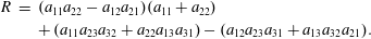 $$\begin{eqnarray}\displaystyle R & = & \displaystyle (a_{11}a_{22}-a_{12}a_{21})(a_{11}+a_{22})\nonumber\\ \displaystyle & & \displaystyle +\,(a_{11}a_{23}a_{32}+a_{22}a_{13}a_{31})-(a_{12}a_{23}a_{31}+a_{13}a_{32}a_{21}).\end{eqnarray}$$
We may thus write
 $Q$
and
$Q$
and
 $R$
as
$R$
as
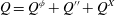 $$\begin{eqnarray}\displaystyle & \displaystyle Q=Q^{\unicode[STIX]{x1D719}}+Q^{\prime \prime }+Q^{X} & \displaystyle\end{eqnarray}$$
 $$\begin{eqnarray}\displaystyle & \displaystyle R=R^{\unicode[STIX]{x1D719}}+R^{\prime \prime }+R^{X}, & \displaystyle\end{eqnarray}$$
in which
 $Q^{\unicode[STIX]{x1D719}}$
and
$Q^{\unicode[STIX]{x1D719}}$
and
 $R^{\prime \prime }$
are invariants computed from the
$R^{\prime \prime }$
are invariants computed from the
 $\unicode[STIX]{x1D622}_{ij}^{\unicode[STIX]{x1D719}}$
and
$\unicode[STIX]{x1D622}_{ij}^{\unicode[STIX]{x1D719}}$
and
 $\unicode[STIX]{x1D622}_{ij}^{\prime \prime }$
fields etc. and
$\unicode[STIX]{x1D622}_{ij}^{\prime \prime }$
fields etc. and
 $Q^{X}$
and
$Q^{X}$
and
 $R^{X}$
are cross-terms that involve contributions from both the
$R^{X}$
are cross-terms that involve contributions from both the
 $\unicode[STIX]{x1D622}_{ij}^{\unicode[STIX]{x1D719}}$
and
$\unicode[STIX]{x1D622}_{ij}^{\unicode[STIX]{x1D719}}$
and
 $\unicode[STIX]{x1D622}_{ij}^{\prime \prime }$
fields. In general these are defined as
$\unicode[STIX]{x1D622}_{ij}^{\prime \prime }$
fields. In general these are defined as
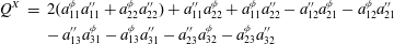 $$\begin{eqnarray}\displaystyle Q^{X} & = & \displaystyle 2(a_{11}^{\unicode[STIX]{x1D719}}a_{11}^{\prime \prime }+a_{22}^{\unicode[STIX]{x1D719}}a_{22}^{\prime \prime })+a_{11}^{\prime \prime }a_{22}^{\unicode[STIX]{x1D719}}+a_{11}^{\unicode[STIX]{x1D719}}a_{22}^{\prime \prime }-a_{12}^{\prime \prime }a_{21}^{\unicode[STIX]{x1D719}}-a_{12}^{\unicode[STIX]{x1D719}}a_{21}^{\prime \prime }\nonumber\\ \displaystyle & & \displaystyle -\,a_{13}^{\prime \prime }a_{31}^{\unicode[STIX]{x1D719}}-a_{13}^{\unicode[STIX]{x1D719}}a_{31}^{\prime \prime }-a_{23}^{\prime \prime }a_{32}^{\unicode[STIX]{x1D719}}-a_{23}^{\unicode[STIX]{x1D719}}a_{32}^{\prime \prime }\end{eqnarray}$$
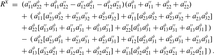 $$\begin{eqnarray}\displaystyle R^{X} & = & \displaystyle (a_{11}^{\prime \prime }a_{22}^{\unicode[STIX]{x1D719}}+a_{11}^{\unicode[STIX]{x1D719}}a_{22}^{\prime \prime }-a_{12}^{\prime \prime }a_{21}^{\unicode[STIX]{x1D719}}-a_{12}^{\unicode[STIX]{x1D719}}a_{21}^{\prime \prime })(a_{11}^{\unicode[STIX]{x1D719}}+a_{11}^{\prime \prime }+a_{22}^{\unicode[STIX]{x1D719}}+a_{22}^{\prime \prime })\nonumber\\ \displaystyle & & \displaystyle +\,(a_{11}^{\unicode[STIX]{x1D719}}[a_{23}^{\prime \prime }a_{32}^{\unicode[STIX]{x1D719}}+a_{23}^{\prime \prime }a_{32}^{\prime \prime }+a_{23}^{\unicode[STIX]{x1D719}}a_{32}^{\prime \prime }]+a_{11}^{\prime \prime }[a_{23}^{\unicode[STIX]{x1D719}}a_{32}^{\unicode[STIX]{x1D719}}+a_{23}^{\unicode[STIX]{x1D719}}a_{32}^{\prime \prime }+a_{23}^{\prime \prime }a_{32}^{\unicode[STIX]{x1D719}}]\nonumber\\ \displaystyle & & \displaystyle +\,a_{22}^{\unicode[STIX]{x1D719}}[a_{13}^{\prime \prime }a_{31}^{\unicode[STIX]{x1D719}}+a_{13}^{\prime \prime }a_{31}^{\prime \prime }+a_{13}^{\unicode[STIX]{x1D719}}a_{31}^{\prime \prime }]+a_{22}^{\prime \prime }[a_{13}^{\unicode[STIX]{x1D719}}a_{31}^{\unicode[STIX]{x1D719}}+a_{13}^{\unicode[STIX]{x1D719}}a_{31}^{\prime \prime }+a_{13}^{\prime \prime }a_{31}^{\unicode[STIX]{x1D719}}])\nonumber\\ \displaystyle & & \displaystyle -\,(a_{12}^{\unicode[STIX]{x1D719}}[a_{23}^{\prime \prime }a_{31}^{\unicode[STIX]{x1D719}}+a_{23}^{\prime \prime }a_{31}^{\prime \prime }+a_{23}^{\unicode[STIX]{x1D719}}a_{31}^{\prime \prime }]+a_{12}^{\prime \prime }[a_{23}^{\unicode[STIX]{x1D719}}a_{31}^{\unicode[STIX]{x1D719}}+a_{23}^{\unicode[STIX]{x1D719}}a_{31}^{\prime \prime }+a_{23}^{\prime \prime }a_{31}^{\unicode[STIX]{x1D719}}]\nonumber\\ \displaystyle & & \displaystyle +\,a_{13}^{\unicode[STIX]{x1D719}}[a_{32}^{\prime \prime }a_{21}^{\unicode[STIX]{x1D719}}+a_{32}^{\prime \prime }a_{21}^{\prime \prime }+a_{32}^{\unicode[STIX]{x1D719}}a_{21}^{\prime \prime }]+a_{13}^{\prime \prime }[a_{32}^{\unicode[STIX]{x1D719}}a_{21}^{\unicode[STIX]{x1D719}}+a_{32}^{\unicode[STIX]{x1D719}}a_{21}^{\prime \prime }+a_{32}^{\prime \prime }a_{21}^{\unicode[STIX]{x1D719}}]).\end{eqnarray}$$
Our particular flow is well approximated as being statistically two-dimensional meaning that there are no gradients of the coherent motions in the
 $z$
-direction nor a velocity component
$z$
-direction nor a velocity component
 $w^{\unicode[STIX]{x1D719}}$
hence (4.8) and (4.9) may be simplified to
$w^{\unicode[STIX]{x1D719}}$
hence (4.8) and (4.9) may be simplified to
 $$\begin{eqnarray}\displaystyle & \displaystyle Q_{2D}^{X}=2(a_{11}^{\unicode[STIX]{x1D719}}a_{11}^{\prime \prime }+a_{22}^{\unicode[STIX]{x1D719}}a_{22}^{\prime \prime })+a_{11}^{\prime \prime }a_{22}^{\unicode[STIX]{x1D719}}+a_{11}^{\unicode[STIX]{x1D719}}a_{22}^{\prime \prime }-a_{12}^{\prime \prime }a_{21}^{\unicode[STIX]{x1D719}}-a_{12}^{\unicode[STIX]{x1D719}}a_{21}^{\prime \prime } & \displaystyle\end{eqnarray}$$
 $$\begin{eqnarray}\displaystyle R_{2D}^{X} & = & \displaystyle (a_{11}^{\prime \prime }a_{22}^{\unicode[STIX]{x1D719}}+a_{11}^{\unicode[STIX]{x1D719}}a_{22}^{\prime \prime }-a_{12}^{\prime \prime }a_{21}^{\unicode[STIX]{x1D719}}-a_{12}^{\unicode[STIX]{x1D719}}a_{21}^{\prime \prime })(a_{11}^{\unicode[STIX]{x1D719}}+a_{11}^{\prime \prime }+a_{22}^{\unicode[STIX]{x1D719}}+a_{22}^{\prime \prime })\nonumber\\ \displaystyle & & \displaystyle +\,a_{11}^{\unicode[STIX]{x1D719}}a_{23}^{\prime \prime }a_{32}^{\prime \prime }-a_{12}^{\unicode[STIX]{x1D719}}a_{23}^{\prime \prime }a_{31}^{\prime \prime }-a_{21}^{\unicode[STIX]{x1D719}}a_{13}^{\prime \prime }a_{32}^{\prime \prime }+a_{22}^{\unicode[STIX]{x1D719}}a_{13}^{\prime \prime }a_{31}^{\prime \prime }.\end{eqnarray}$$
Nevertheless, to avoid further assumptions we shall persist with the definitions of
 $Q^{X}$
and
$Q^{X}$
and
 $R^{X}$
from (4.8) and (4.9), cognisant of the fact that terms such as
$R^{X}$
from (4.8) and (4.9), cognisant of the fact that terms such as
 $a_{13}^{\unicode[STIX]{x1D719}}\approx 0$
.
$a_{13}^{\unicode[STIX]{x1D719}}\approx 0$
.


Figure 9 illustrates the joint p.d.f.s between
 $Q^{X}$
and
$Q^{X}$
and
 $R^{X}$
, as defined in (4.8) and (4.9) respectively, at the various streamwise locations highlighted in figure 5 along the centreline (a) and the shear layer (b). The joint p.d.f.s are computed from the same
$R^{X}$
, as defined in (4.8) and (4.9) respectively, at the various streamwise locations highlighted in figure 5 along the centreline (a) and the shear layer (b). The joint p.d.f.s are computed from the same
 $0.13D\times 0.13D$
interrogation windows as before, the contour levels are again chosen such that
$0.13D\times 0.13D$
interrogation windows as before, the contour levels are again chosen such that
 $\unicode[STIX]{x1D6F4}=0.683$
and the axes are normalised by
$\unicode[STIX]{x1D6F4}=0.683$
and the axes are normalised by
 $\langle Q_{\unicode[STIX]{x1D714}}\rangle (x)$
. Whilst the shape of the contours does not exactly resemble the classical ‘tear drop’ shape of
$\langle Q_{\unicode[STIX]{x1D714}}\rangle (x)$
. Whilst the shape of the contours does not exactly resemble the classical ‘tear drop’ shape of
 $f_{QR}(Q,R)$
, in particular the Vieillefosse tail is absent, some features are present. These include the predominance of states for which
$f_{QR}(Q,R)$
, in particular the Vieillefosse tail is absent, some features are present. These include the predominance of states for which
 $\unicode[STIX]{x1D6E5}>0$
(swirling), the enhancement of sector
$\unicode[STIX]{x1D6E5}>0$
(swirling), the enhancement of sector
 $I$
(primarily responsible for enstrophy amplification) and the narrowed sector
$I$
(primarily responsible for enstrophy amplification) and the narrowed sector
 $II$
(primarily responsible for enstrophy attenuation). Further, it can be seen that all of the contour levels collapse well with each other, particularly from the rear face of the cylinder up until the location of the peak turbulence intensity.
$II$
(primarily responsible for enstrophy attenuation). Further, it can be seen that all of the contour levels collapse well with each other, particularly from the rear face of the cylinder up until the location of the peak turbulence intensity.
The shape of the joint p.d.f. contours of figure 9 look remarkably similar to
 $f_{QR}(Q,R)$
extracted from the closest location to the turbulence generating grid of Gomes-Fernandes et al. (Reference Gomes-Fernandes, Ganapathisubramani and Vassilicos2014). It was in this region of the flow that Gomes-Fernandes et al. (Reference Gomes-Fernandes, Ganapathisubramani and Vassilicos2015) observed an inverse cascade of turbulent kinetic energy, along a particular axis, which was partly attributed to the multi-scale nature of the flow generated by their particular space-filling fractal square grid. This region of the flow was termed the turbulence production region since
$f_{QR}(Q,R)$
extracted from the closest location to the turbulence generating grid of Gomes-Fernandes et al. (Reference Gomes-Fernandes, Ganapathisubramani and Vassilicos2014). It was in this region of the flow that Gomes-Fernandes et al. (Reference Gomes-Fernandes, Ganapathisubramani and Vassilicos2015) observed an inverse cascade of turbulent kinetic energy, along a particular axis, which was partly attributed to the multi-scale nature of the flow generated by their particular space-filling fractal square grid. This region of the flow was termed the turbulence production region since
 $u_{rms}^{\prime }$
was an increasing function of
$u_{rms}^{\prime }$
was an increasing function of
 $x$
. In such a flow the coherent dynamics of the bars of various length scales interacted with each other, and the background incoherent turbulence. It may thus be hypothesised that the cross-terms,
$x$
. In such a flow the coherent dynamics of the bars of various length scales interacted with each other, and the background incoherent turbulence. It may thus be hypothesised that the cross-terms,
 $Q^{X}$
and
$Q^{X}$
and
 $R^{X}$
, were important in this region of the flow which perhaps explains the resemblance of
$R^{X}$
, were important in this region of the flow which perhaps explains the resemblance of
 $f_{QR}(Q,R)$
to figure 9.
$f_{QR}(Q,R)$
to figure 9.
Joint p.d.f.s between
 $-\unicode[STIX]{x1D634}_{ij}\unicode[STIX]{x1D634}_{jk}\unicode[STIX]{x1D634}_{ki}$
, the strain self-amplification rate, and
$-\unicode[STIX]{x1D634}_{ij}\unicode[STIX]{x1D634}_{jk}\unicode[STIX]{x1D634}_{ki}$
, the strain self-amplification rate, and
 $\unicode[STIX]{x1D714}_{i}\unicode[STIX]{x1D634}_{ij}\unicode[STIX]{x1D714}_{j}$
, the enstrophy amplification rate along the centreline of the flow computed from the
$\unicode[STIX]{x1D714}_{i}\unicode[STIX]{x1D634}_{ij}\unicode[STIX]{x1D714}_{j}$
, the enstrophy amplification rate along the centreline of the flow computed from the
 $\unicode[STIX]{x1D622}_{ij}^{\unicode[STIX]{x1D719}}$
field (a) and the
$\unicode[STIX]{x1D622}_{ij}^{\unicode[STIX]{x1D719}}$
field (a) and the
 $\unicode[STIX]{x1D622}_{ij}^{\prime \prime }$
field (b). The dashed line marks
$\unicode[STIX]{x1D622}_{ij}^{\prime \prime }$
field (b). The dashed line marks
 $\unicode[STIX]{x1D714}_{i}\unicode[STIX]{x1D634}_{ij}\unicode[STIX]{x1D714}_{j}=-4/3\unicode[STIX]{x1D634}_{ij}\unicode[STIX]{x1D634}_{jk}\unicode[STIX]{x1D634}_{ki}$
and thus data from below the line correspond to
$\unicode[STIX]{x1D714}_{i}\unicode[STIX]{x1D634}_{ij}\unicode[STIX]{x1D714}_{j}=-4/3\unicode[STIX]{x1D634}_{ij}\unicode[STIX]{x1D634}_{jk}\unicode[STIX]{x1D634}_{ki}$
and thus data from below the line correspond to
 $R<0$
whilst the data above the line correspond to
$R<0$
whilst the data above the line correspond to
 $R>0$
. The contour colours correspond to the streamwise locations depicted in figure 5.
$R>0$
. The contour colours correspond to the streamwise locations depicted in figure 5.
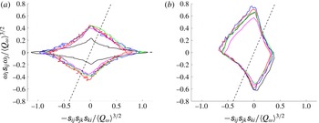
In the transport equations for
 $\unicode[STIX]{x1D714}^{2}$
and
$\unicode[STIX]{x1D714}^{2}$
and
 $\unicode[STIX]{x1D634}_{ij}\unicode[STIX]{x1D634}_{ij}$
the inviscid source terms are
$\unicode[STIX]{x1D634}_{ij}\unicode[STIX]{x1D634}_{ij}$
the inviscid source terms are
 $\unicode[STIX]{x1D714}_{i}\unicode[STIX]{x1D634}_{ij}\unicode[STIX]{x1D714}_{j}$
(in the enstrophy equation) and
$\unicode[STIX]{x1D714}_{i}\unicode[STIX]{x1D634}_{ij}\unicode[STIX]{x1D714}_{j}$
(in the enstrophy equation) and
 $-\unicode[STIX]{x1D634}_{ij}\unicode[STIX]{x1D634}_{jk}\unicode[STIX]{x1D634}_{ki}$
and
$-\unicode[STIX]{x1D634}_{ij}\unicode[STIX]{x1D634}_{jk}\unicode[STIX]{x1D634}_{ki}$
and
 $-\unicode[STIX]{x1D714}_{i}\unicode[STIX]{x1D634}_{ij}\unicode[STIX]{x1D714}_{j}$
(in the strain-rate equation). Clearly
$-\unicode[STIX]{x1D714}_{i}\unicode[STIX]{x1D634}_{ij}\unicode[STIX]{x1D714}_{j}$
(in the strain-rate equation). Clearly
 $\unicode[STIX]{x1D714}_{i}\unicode[STIX]{x1D634}_{ij}\unicode[STIX]{x1D714}_{j}$
is thus a source of enstrophy and a sink for dissipation, and these two terms are the constituents of
$\unicode[STIX]{x1D714}_{i}\unicode[STIX]{x1D634}_{ij}\unicode[STIX]{x1D714}_{j}$
is thus a source of enstrophy and a sink for dissipation, and these two terms are the constituents of
 $R$
as outlined in (1.4). Figure 10 shows joint p.d.f.s, again with contour levels set such that
$R$
as outlined in (1.4). Figure 10 shows joint p.d.f.s, again with contour levels set such that
 $\unicode[STIX]{x1D6F4}=0.683$
, between
$\unicode[STIX]{x1D6F4}=0.683$
, between
 $\unicode[STIX]{x1D714}_{i}\unicode[STIX]{x1D634}_{ij}\unicode[STIX]{x1D714}_{j}$
and
$\unicode[STIX]{x1D714}_{i}\unicode[STIX]{x1D634}_{ij}\unicode[STIX]{x1D714}_{j}$
and
 $-\unicode[STIX]{x1D634}_{ij}\unicode[STIX]{x1D634}_{jk}\unicode[STIX]{x1D634}_{ki}$
computed along the centreline from the
$-\unicode[STIX]{x1D634}_{ij}\unicode[STIX]{x1D634}_{jk}\unicode[STIX]{x1D634}_{ki}$
computed along the centreline from the
 $\unicode[STIX]{x1D622}_{ij}^{\unicode[STIX]{x1D719}}$
field (a) and the
$\unicode[STIX]{x1D622}_{ij}^{\unicode[STIX]{x1D719}}$
field (a) and the
 $\unicode[STIX]{x1D622}_{ij}^{\prime \prime }$
field (b). The remarkable collapse of the joint p.d.f.s of figure 6 can perhaps be explained by the self-preserving nature of the statistical distributions of these inviscid source/sink terms, which drive the evolution of enstrophy and dissipation. With the exception of the contour taken immediately downstream of the cylinder for the coherent velocity-gradient tensor field, in which
$\unicode[STIX]{x1D622}_{ij}^{\prime \prime }$
field (b). The remarkable collapse of the joint p.d.f.s of figure 6 can perhaps be explained by the self-preserving nature of the statistical distributions of these inviscid source/sink terms, which drive the evolution of enstrophy and dissipation. With the exception of the contour taken immediately downstream of the cylinder for the coherent velocity-gradient tensor field, in which
 $\langle Q_{\unicode[STIX]{x1D714}}\rangle$
is small, the contours collapse onto one another. There is a clear qualitative difference in the distributions for both. There is a preference for the production of enstrophy alongside mild (inviscid) production of dissipation in the field of stochastic velocity fluctuations. Intuitively, this would be required for an inhomogeneous flow to evolve into a ‘fully developed’ flow, in which the fine-scale structure is observed to consist of tubes of intense enstrophy surrounded by more extensive sheets of dissipation. The opposite trend is observed in the field of coherent fluctuations, in which the inviscid production of dissipation is favoured, which again one might expect considering the decreasing significance of the coherent motions with streamwise distance in a turbulent shear flow.
$\langle Q_{\unicode[STIX]{x1D714}}\rangle$
is small, the contours collapse onto one another. There is a clear qualitative difference in the distributions for both. There is a preference for the production of enstrophy alongside mild (inviscid) production of dissipation in the field of stochastic velocity fluctuations. Intuitively, this would be required for an inhomogeneous flow to evolve into a ‘fully developed’ flow, in which the fine-scale structure is observed to consist of tubes of intense enstrophy surrounded by more extensive sheets of dissipation. The opposite trend is observed in the field of coherent fluctuations, in which the inviscid production of dissipation is favoured, which again one might expect considering the decreasing significance of the coherent motions with streamwise distance in a turbulent shear flow.
5 Conclusions
Tomographic PIV experiments were performed in the near field of the turbulent flow around a square cylinder generating a 3D3C data set. The velocity field was decomposed, according to (1.5), into a time invariant base flow, a coherent fluctuation and a residual/stochastic fluctuation. This was conducted by means of phase bin averaging in which the phase angle of each instantaneously acquired 3D3C velocity field was calculated from the time-varying mode coefficients of the second and third modes obtained from a proper orthogonal decomposition of the flow field. These two modes correspond to the vortex shedding downstream of the cylinder. From these three separate velocity fields the invariants of the velocity-gradient tensor were computed and their statistics compared to one another. Since the flow is spatially developing and inhomogeneous these statistics were computed both upstream, including from within the mean recirculation region, and downstream of the location of peak turbulence intensity along the centreline of the flow. Additionally, the statistics were extracted from the shear layer region of the flow; so defined as the local maximum in turbulence intensity at a given downstream,
 $x$
, location.
$x$
, location.
Joint p.d.f.s between the rotating and straining constituents of the invariant
 $Q$
,
$Q$
,
 $Q_{\unicode[STIX]{x1D714}}$
and
$Q_{\unicode[STIX]{x1D714}}$
and
 $Q_{s}$
respectively, highlighted the very different flow physics and topologies of the various velocity-gradient fields at the various spatial interrogation locations. Despite the differing flow physics and topologies of the various fields of velocity gradients the joint p.d.f.s between the second and third invariants,
$Q_{s}$
respectively, highlighted the very different flow physics and topologies of the various velocity-gradient fields at the various spatial interrogation locations. Despite the differing flow physics and topologies of the various fields of velocity gradients the joint p.d.f.s between the second and third invariants,
 $Q$
and
$Q$
and
 $R$
resembled the classical ‘tear drop’ shapes associated with fully developed turbulence when computed from the total and stochastic velocity gradients. In fact the contours of the joint p.d.f.s were found to collapse in a self-similar fashion when appropriately normalised by the local ensemble average of
$R$
resembled the classical ‘tear drop’ shapes associated with fully developed turbulence when computed from the total and stochastic velocity gradients. In fact the contours of the joint p.d.f.s were found to collapse in a self-similar fashion when appropriately normalised by the local ensemble average of
 $Q_{\unicode[STIX]{x1D714}}$
. Such self-similar ‘tear drop’ shapes were found along the centreline and the shear layer at all but the farthest downstream locations. Observation of the relative magnitudes of the rotationally dominated sectors
$Q_{\unicode[STIX]{x1D714}}$
. Such self-similar ‘tear drop’ shapes were found along the centreline and the shear layer at all but the farthest downstream locations. Observation of the relative magnitudes of the rotationally dominated sectors
 $I$
and
$I$
and
 $II$
showed that these tended to be in balance with one another and only very slowly variant in space, although their values did change according to which velocity-gradient field they were computed from. The statistics of the inviscid source/sink terms in the evolution of the enstrophy and dissipation are observed to also collapse remarkably well with the local value of
$II$
showed that these tended to be in balance with one another and only very slowly variant in space, although their values did change according to which velocity-gradient field they were computed from. The statistics of the inviscid source/sink terms in the evolution of the enstrophy and dissipation are observed to also collapse remarkably well with the local value of
 $\langle Q_{\unicode[STIX]{x1D714}}\rangle$
, offering a potential explanation for the collapse of the ‘tear drop’-shaped joint p.d.f.s. As expected the joint p.d.f.s computed from the coherent velocity gradients did not resemble those from fully developed turbulence.
$\langle Q_{\unicode[STIX]{x1D714}}\rangle$
, offering a potential explanation for the collapse of the ‘tear drop’-shaped joint p.d.f.s. As expected the joint p.d.f.s computed from the coherent velocity gradients did not resemble those from fully developed turbulence.
It thus seems that the ubiquitous ‘tear drop’-shaped statistical distribution of the invariants of the velocity-gradient tensor is even more ubiquitous than first thought. Not only does it appear in a manner of (homogeneous) fully developed turbulent flows, but this manuscript also shows that it exists in inhomogeneous flows with rapidly spatially varying flow physics. Whilst fully developed flows have a flat spectrum of turbulent kinetic energy at the low wavenumbers the flow past a square cylinder has a clear spike at the vortex shedding wavenumber. From this perspective we should thus consider the ‘tear drop’-shaped joint p.d.f. between the invariants of the velocity-gradient tensor not as a universal feature of fully developed turbulence (Chacin & Cantwell Reference Chacin and Cantwell2000; Elsinga & Marusic Reference Elsinga and Marusic2010) but as a universal feature of turbulent flows.
Acknowledgements
O.B. would like to acknowledge Dr G. Elsinga for graciously hosting him for the acquisition of the data during a visit to TU Delft in September 2014 and Dr D. Michaelis for assistance with processing the tomographic PIV data. O.B. and M.B. would like to acknowledge funding through EPSRC grant no. EP/L023520/1. O.B. would also like to thank Dr C. Keylock for a fruitful discussion whilst preparing a revised version of the manuscript.


 Open access