
Implications
Genetic diseases arise regularly in animal populations due to naturally occurring random changes to the genome (mutations). To remove the effect of new variants from the population, one must find their cause. Reports from successful experiments indicate that a method based on using genome markers to highlight long identical stretches of an animal’s chromosome pairs is most successful. Subsequently, reading the whole genome of a small number of affected animals, and their parents, should allow the exact location of the variant to be known and a genetic test devised to find all animals carrying the variant in the population.
Introduction
Any researcher faced with the advent of a new autosomal recessive genetic disease has a number of problems to solve in order to find the cause of the new condition and then devise a suitable test to control the effect of the new variant in the population. The review, described later in this paper, found many instances where the characteristics of the condition suggested a candidate gene which may be responsible for the condition, either from the symptoms being shown by the animal or from similarity with other known genetic diseases in other breeds or species. The methods reviewed in this paper apply to new conditions which do not involve such a candidate gene, and so the gene or region of the genome involved is unknown at the outset.
A common scenario is that a small number of cases become evident in a population over a few years; thus power requirements are often limited. In addition, cases are likely to be more inbred than a similar sized group randomly selected from the rest of the population and so there may be two causes of ‘excessive’ homozygosity in the genome of cases, the site of the new variant and/or a more general increased level of inbreeding due to the relatedness of their parents. Assuming that the autosomal recessive mode of inheritance has already been worked out by pedigree and segregation analysis and a similar condition has not already been found in another breed or species suggesting a candidate gene, then the task is to use that information, together with some form of genotyping, to find the signals relevant to the new variant at a particular place on the genome. The region of the genome containing the new variant (the target region) must be located before ‘fine mapping’ that area to identify possible causal variants and hence derive a genetic test to identify carriers and potential cases in the instance of a late-onset condition. An alternative approach may be to identify a haplotype associated with the new variant using suitable classification methods based on single nucleotide polymorphism (SNP) genotypes (see Biscarini et al., Reference Biscarini, Schwarzenbacher, Pausch, Nicolazzi, Pirola and Biffani2016 as an example). Then, this test should be used to screen the population and instigate a suitable breeding programme.
This paper will review the bioinformatic methodology, used to map a new autosomal recessive disorder, in a number of ways. First, recent reports of such papers will be summarised and the methods used highlighted. Then the commonly used methods will be compared on a data set with a known outcome in order to see how they perform. In addition, an alternative method will be proposed and compared with those already used in the literature. Finally, ‘fine-mapping’ methodology from the literature review will be compared and some new insights into whole genome sequencing (WGS), as an aid to find a new variant, will be discussed.
The autosomal recessive condition
New mutations are a regular phenomenon in any animal species and a new autosomal recessive condition will arise when such a variant occurs in a part of the genome which clearly has an impact on the phenotype of the animal when both chromosomes carry an identical version of it. This process is illustrated in Figure 1 for a simple autosomal recessive condition. More complex modes of inheritance, such as that involving two (or more) genes, sex-linkage or compound heterozygosity, will have a more complicated pattern of gene flow. One consequence of the autosomal recessive condition requiring two copies of the variant for it to occur is that each copy of the variant will bring with it a haplotype from the original chromosome where the mutation occurred. Thus, around the variant, there will be identical lengths of sequence which will result in runs of homozygosity (ROH), only limited in length by recombination events occurring either side of the new variant, by chance. At the variant site all cases will be homozygous for the same variant sequence and all parents of cases will be heterozygous, including this variant sequence, as well. All other controls could be either homozygous for an alternative base (or bases) or heterozygotes; they are referred to as carriers if they are heterozygous and contain the variant (see Figure 1).
The advent of a new autosomal recessive genetic condition on a single pair of homologous chromosomes followed over several generations.

Methods found in a sample survey of the literature
Initial step
Since the advent of SNP-chip technology, a number of examples of bioinformatic methods to help solve the problem of mapping a new variant have been used. The papers summarised in the Supplementary Tables S1 and S2 were a random 50% sample from the Online Mendelian Inheritance in Animals database (Online Mendelian Inheritance in Animals, 2017) using the search terms ‘autosomal recessive’, for mode of inheritance, and ‘key mutation known’ for cattle, horse, sheep, chicken and pig. Papers where a candidate gene or similar condition had already been identified in another breed or species were ignored. The Supplementary Tables S1 and S2 summarise the methods used in 34 resultant papers, containing 38 disorders, whose references are shown in the Supplementary Material S1. References to all the software quoted throughout this paper, and shown as capitalised in the text, are given in the Supplementary Table S3. Methods based on exome sequencing (e.g. Krauthammer et al., Reference Krauthammer, Kong, Hak Ha, Evans, Bacchiocchi, McCusker, Cheng, Davis, Goh, Choi, Ariyan, Narayan, Dutton-Regester, Capatana, Holman, Bosenberg, Sznol, Kluger, Brash, Stern, Materin, Lo, Mane, Ma, Kidd, Hayward, Lifton, Schlessinger, Boggon and Halaban2012), candidate genes (e.g. Michot et al., Reference Michot, Fritz, Barbat, Boussaha, Deloche, Grohs, Hoze, Le Berre, Le Bourhis, Desnoes, Salvetti, Schibler, Boichard and Capitan2017), homology (e.g. Tan et al., 1997) or missing homozygosity (e.g. Van Raden et al., Reference VanRaden, Olson, Null and Hutchison2011) have been ignored in this paper as they can rarely be applied to the novel autosomal recessive scenario under review here, or only cover a limited proportion of the genome (exomes comprise >2% of the genome; International Human Genome Sequencing Consortium, 2004).
The commonly used methods to find the region containing a new autosomal recessive variant involving genomewide SNP data can be categorised into two groups based on either a range of χ 2 tests or ROH. The logic behind each approach is very different. In χ 2-based methods, each SNP is analysed separately with one or more of an allelic, genotypic, dominant or recessive model and the departure of the results from the expected distribution of the cases and controls, based on the marginal values, signals a SNP of interest (see Supplementary Material S2 for an explanation of these models). Appropriate correction for multiple testing is required to pinpoint the genomic area of interest, or the use of Fisher’s exact test if expected numbers are <5, in any cell of the contingency table. The ROH approach takes the view that the new autosomal recessive variant will be characterised by a long ROH, as described above (see Figure 1). These are likely to be few in the case of a new genetic disease so by searching for the longest ROH found in all cases, then the site of the new disease should be found.
The commonly used methods found in the papers reviewed can be summarised as χ 2 or Fisher’s Exact test (16 examples: 11 allelic, three recessive, one genotypic model and one novel method), homozygosity mapping in PLINK (13), ASSHOM/ASSIST (11), haplotype analysis with BEAGLE (five) or HAPLOVIEW (two), some form of mixed model (four) and the paper’s authors own method (two). The mixed model analyses used GCTA, GenAbel and ASReml, where a method was quoted. In addition, Venhoranta et al. (Reference Venhoranta, Pausch, Flisikowski, Wurmser, Taponen, Rautala, Kind, Schnieke, Fries, Lohi and Andersson2014) used a novel sliding window approach with Fisher’s Exact test. Twenty-two of the reports used two or more methods in the initial step either as a two-stage approach, where a larger region found with the first stage was refined with the second method, or where two methods were used independently and overlapping regions highlighted. The χ 2 method was always used in conjunction with another method, usually as the first step, with one exception (Finno et al., Reference Finno, Stevens, Young, Affolter, Joshi, Ramsay and Bannasch2015) when it was the only method reported. Of the two methods designed by Charlier et al. (Reference Charlier, Coppieters, Rollin, Desmecht, Agerholm, Cambisano, Carta, Dardano, Dive, Fasquelle, Frennet, Hanset, Hubin, Jorgensen, Karim, Kent, Harvey, Pearce, Simon, Tama, Nie, Vandeputte, Lien, Longeri, Fredholm, Harvey and Georges2008), ASSHOM was used more frequently than ASSIST but these methods were generally used on their own. Only two authors reported that a method failed to work, Rafati et al. (Reference Rafati, Andersson, Mikko, Feng, Raudsepp, Pettersson, Janecka, Wattle, Ameur, Thyreen, Eberth, Huddleston, Malig, Bailey, Eichler, Dalin, Chowdary, Anderssson, Lindgren and Rubin2016; method not quoted) and Waide et al. (Reference Waide, Dekkers, Ross, Rowland, Wyatt, Ewen, Evans, Thekkoot, Boddicker, Serão, Ellinwood and Tuggle2015; ROH method using –homozyg in PLINK).
The number of cases and controls does not appear to be an issue, with ratios as low as 3:4 (cases:controls) being reported. Mean group sizes were 21 and 53 animals for cases and controls, with median values of 12 and 27, respectively. Because of the nature of new genetic diseases, these tended to be small studies. Of course, ROH methods rely on the random occurrence of recombinations close to the variant in order to be successful and so having more cases is likely to be more useful for these methods.
The number of SNP used in the reviewed studies ranged from 13 000 to 777 000 and was more a function of the commercially available chips than anything relating to the requirements for success of the methods. However, it seems logical to use as dense a SNP panel as possible to pick up more subtle changes in ROH lengths. The mean length of the target regions identified in the 38 genetic diseases was 4.6 megabases (Mb) with a range of 0.61 to 21.5 Mb and a median value of 2.5 Mb. Nine authors reported the identified region at both stages of a two-stage approach, usually χ 2 followed by a ROH method; the reduction in region between the two stages due to the use of the second method was 9.6 Mb on average.
Final step
The papers reviewed above indicate that using SNP data can only locate a new variant to within about a 4.6 Mb region of the genome on average. Nearly all the papers summarised in the Supplementary Table S1 went on to locate the actual variant using further methods (Supplementary Table S2). In all, 18 of these papers looked for candidate genes located in the target region using a suitable database and either resequenced them all or the most likely one, based on the biology of the condition and the function of the genes found in the target region. A total of 11 reports used WGS on a small number of cases and controls and searched within the target region for likely base positions, being identically homozygous in all cases and not in controls. Two reports used exome sequencing within the target region and further two resequenced the complete target region. One report used reverse transcription in cases and controls and compared the products, whereas the other report compared expression levels of genes in the target area.
Clearly, there is no one favoured approach to finding the new variant within the target area and all required somewhat complicated and/or expensive methods to achieve a result.
Initial step methods compared on the Lavender Foal Syndrome data set
This paper reviews different ‘readily available’ SNP-based methods for mapping the target region containing the new causal variant of an autosomal recessive condition by comparing their outcomes using a single data set. A range of methods were compared using the data set of Brooks et al. (Reference Brooks, Gabreski, Miller, Brisbin, Brown, Streeter, Mezey, Cook and Antczak2010) who identified the site of the Lavender Foal Syndrome (LFS) variant using 36 horses and the EquCab2.0 build of the equine genome. They found the location of this genetic disorder in foals using a combination of χ 2 test and haplotype analysis, in HAPLOVIEW, to locate the likely region containing the variant and sequencing of a positional candidate gene to refine the site of the disease within the identified region. This was shown to be a single base deletion on chromosome 1 of the horse (ECA1) in the MYO5A gene. This data set comprised 56 541 SNP from six affected (cases) and 30 unaffected individuals (controls) derived using the Illumina EquineSNP50 chip. All SNP locations used refer to the EquCab2.0 build of the horse genome.
χ 2 Method
The χ 2 approach can be found in free software packages such as R (R Core Team, 2013) or PLINK (Purcell et al., Reference Purcell, Neale, Todd-Brown, Thomas, Ferreira, Bender, Maller, Sklar, de Bakker, Daly and Sham2007). The genotypic χ 2 method implemented in PLINK version 1.9 (Chang et al., Reference Chang, Chow, Tellier, Vattikuti, Purcell and Lee2015) with Fisher’s Exact test was used to generate results, after Brooks et al. (Reference Brooks, Gabreski, Miller, Brisbin, Brown, Streeter, Mezey, Cook and Antczak2010). This method uses the three possible SNP genotypes (say AA, AT and TT) and the two disease states (cases and controls) in a 3×2 table at each SNP. Further models are also implemented in PLINK involving recessive, dominant and allelic models as well as the Cochran–Armitage trend test (see Supplementary Material S2 for a comparison of the four models using the χ 2 tests).
Runs of homozygosity in PLINK
The ‘homozyg-group’ option in PLINK (version 1.9) was used to generate ROH. This method uses a ‘sliding window’ along the length of the genome and scores each window by using the number of homozygous SNP found and only uses cases. As observed by Howrigan et al. (Reference Howrigan, Simonson and Keller2011), the parameters used to define the ROH windows and the use of linkage disequilibrium (LD) pruning appeared to be critical for generating ‘correct’ ROH. Pausch et al. (Reference Pausch, Venhoranta, Wurmser, Hakala, Iso-Touru, Sironen, Vingborg, Lohi, Söderquist, Fries and Andersson2016) stated that ‘Due to the relatively sparse genome coverage of the genotype data (1 SNP per 56 kb), we restricted our analysis to runs of homozygosity with a minimum number of 20 contiguous homozygous SNPs and a minimum length of 500 kb’. They did not appear to use LD pruning. In the current analysis, the SNP with a low genotyping rate were excluded (<0.9) and the parameters were set at a 20-SNP window with a minimum of five adjacent homozygous SNP for a data set with a similar SNP density to that of Pausch et al. (Reference Pausch, Venhoranta, Wurmser, Hakala, Iso-Touru, Sironen, Vingborg, Lohi, Söderquist, Fries and Andersson2016), whose parameters were used here.
Homozygosity scoring methods of Charlier et al. (Reference Charlier, Coppieters, Rollin, Desmecht, Agerholm, Cambisano, Carta, Dardano, Dive, Fasquelle, Frennet, Hanset, Hubin, Jorgensen, Karim, Kent, Harvey, Pearce, Simon, Tama, Nie, Vandeputte, Lien, Longeri, Fredholm, Harvey and Georges2008)
Charlier et al. (Reference Charlier, Coppieters, Rollin, Desmecht, Agerholm, Cambisano, Carta, Dardano, Dive, Fasquelle, Frennet, Hanset, Hubin, Jorgensen, Karim, Kent, Harvey, Pearce, Simon, Tama, Nie, Vandeputte, Lien, Longeri, Fredholm, Harvey and Georges2008) applied two methods to five conditions in cattle and demonstrated success with as few as three cases and nine controls. The Charlier et al. (Reference Charlier, Coppieters, Rollin, Desmecht, Agerholm, Cambisano, Carta, Dardano, Dive, Fasquelle, Frennet, Hanset, Hubin, Jorgensen, Karim, Kent, Harvey, Pearce, Simon, Tama, Nie, Vandeputte, Lien, Longeri, Fredholm, Harvey and Georges2008) approach uses two different scores to locate the variant: a homozygosity score (ASSHOM) and a core-marker score (ASSIST). These scores attempt to utilise the two major characteristics of autosomal recessive variants. First, long ROH are scored. Second, the variant must be at a SNP homozygous for the same genotype in all cases, and this SNP will be in the longest ROH in all or most cases.
The ASSHOM method looks for ROH in cases and scores them on the basis of the allele frequencies found in the controls of the allele involved in the homozygous SNP at each SNP, rarer alleles being given a higher score through the use of −log10(p 2), where p is the allele frequency in controls of the allele forming the homozygous genotype in each case. The ASSIST method looks for SNP which are monomorphic in cases and polymorphic in controls, the so-called ‘core markers’. It then calculates a score for each core marker based on the length of common homozygosity in all cases around this SNP. Again scores are based on the allele frequency, in controls, of the allele contained in the core marker, rarer alleles being given a higher score (−log10(p 2)). It is worth noting that the ASSHOM and ASSIST scores are not easily interpretable units but are used as relative values within any analysis. In both methods heterozygotes are penalised heavily, both by being given a very low score (10−5) and the use of the harmonic mean to calculate each SNP’s overall score.
Autozygosity by difference
A new ROH method was devised to overcome some of the perceived limitations of the published methods (i.e. they all failed to find the region highlighted by Brooks et al. (Reference Brooks, Gabreski, Miller, Brisbin, Brown, Streeter, Mezey, Cook and Antczak2010) after haplotype analysis; see below). In addition, it was designed to help overcome issues of incomplete penetrance, late-onset conditions, higher levels of inbreeding, misgenotyping and breed-specific ROH (see the ‘Discussion’ section below for an explanation). This method calculates ROH lengths in both cases and controls and uses the difference between mean ROH length at each SNP in cases and controls as the signal for mapping the variant; hence the name autozygosity by difference (ABD), this difference being the ABD score. The overall approach in the ABD method is to search for ROH with the appropriate characteristics. The appropriate characteristics are the longest ROH found to contain an identical haplotype in all cases, but accounting for any similar ROH in the controls. In livestock species there may be breed-specific ROH which are associated with breed characteristics, which need to be taken into account. The genome positions with the highest ABD score indicate where a causal variant is most likely to be found. Thus scoring for ROH occurs in both cases and controls. In the ABD method, each animal is scored at each SNP on all chromosomes as detailed in Supplementary Material S3. Previous preliminary studies using this method during its development have been reported by Pollott (Reference Pollott2012) and Biscarini et al. (Reference Biscarini, Del Corvo, Stella, Albera, Ferenčaković and Pollott2013).
Probability by permutation
When using SNP-based methods, the same data set is used repeatedly up to the number of SNP available and so correction for multiple testing is an issue. Typically in this situation the Bonferroni correction might be used to control for false positives. Geneticists have tended to avoid this method as it is ultraconservative and discounts the results in many studies. The common software packages used to find the site of a new autosomal recessive variant contain a number of alternative approaches based on permutation, although the summary of papers reviewed in the Supplementary Table S1 only found seven out of 34 papers which used permutation and only six which quoted permuted probabilities. No other multiple-testing correction method was found.
PLINK contains a number of options for varying the Monte Carlo permutation method (PLINK, 2007). These are label-swapping or gene-dropping methods used within either adaptive or max(T) permutation. The Monte Carlo method used to calculate the Fisher’s Exact test is in itself a permutation procedure. Most studies reviewed in the Supplementary Table S1 which used permutation testing employed label-swapping procedures. The methodology for χ 2 analyses by each SNP in turn label-swaps within each SNP. This contrasts with the ASSHOM, ASSIST and ABD methods which either label-swap at the whole genome level (ASSIST, ABD), effectively reassigning animals randomly to phenotypes and recalculating the results, or by SNP (ASSHOM), which breaks LD and ROH for permutation purposes. There appears to be no consistency in the number of permutations used. The reviewed papers used anything from 10 000 to 1 million permutations.
The LFS data set was analysed using a range of permutations from 1 to 500 000 using a χ 2 genotypic model and the results were summarised into three bands; the number of SNP found to be significant at the P=0.05, 0.01 and 0.001 levels.
Outcome of initial step methods using the Lavender Foal Syndrome data set
A summary of the results from all the methods compared is shown in Table 1.
Summary of the five methods using the Lavender Foal Syndrome data set of Brooks et al. (Reference Brooks, Gabreski, Miller, Brisbin, Brown, Streeter, Mezey, Cook and Antczak2010) based on the horse genome build EquCab 2.0

SNP=single nucleotide polymorphism; Mb=megabases; ECA=horse chromosome number; ABD=autozygosity by difference.
1 ASSIST – not a continuous run – longest run three SNPs only.
2 ASSIST longest run – didn’t include the actual variant.
χ 2 results
The results of Brooks et al. (Reference Brooks, Gabreski, Miller, Brisbin, Brown, Streeter, Mezey, Cook and Antczak2010) were repeated using the χ 2 test in PLINK on a 3×2 genotype×disease status table using Fisher’s Exact test (Supplementary Figure S1 and Table 1) but with no editing of the SNP for minor allele frequency (MAF). Significance levels quoted were from a χ 2 distribution with 2 degrees of freedom and the Bonferroni correction was applied using 36 651 informative SNP. Brooks et al. (Reference Brooks, Gabreski, Miller, Brisbin, Brown, Streeter, Mezey, Cook and Antczak2010), using the EquCab2.0 build of the horse genome, identified ‘14 highly significant SNPs encompassed a region spanning 10.5 Mb (ECA1:129 228 091 to 139 718 117)’. They also found four unique haplotypes in the six cases in this region using HAPLOVIEW. Within these four haplotypes, there was one block of 27 SNP which was homozygous in all cases covering a 1.56-Mb region. Subsequent candidate gene sequencing in this region by Brooks et al. (Reference Brooks, Gabreski, Miller, Brisbin, Brown, Streeter, Mezey, Cook and Antczak2010) finally discovered the causal variant to be a single base deletion located at base position 138 235 715, in the MYO5A gene. In the context of the current comparison between methods, these results are crucial. One aim of this paper is to compare the available methods for locating the region containing a new autosomal recessive variant using the data of Brooks et al. (Reference Brooks, Gabreski, Miller, Brisbin, Brown, Streeter, Mezey, Cook and Antczak2010). The major criterion for assessing a method is that it found the same 1.56 Mb region, or narrower, containing the base position (ECA1:138 235 715) highlighted by Brooks et al. (Reference Brooks, Gabreski, Miller, Brisbin, Brown, Streeter, Mezey, Cook and Antczak2010) as the causal variant of LFS. Table 1 summarises the key results from all compared methods and shows the results of Brooks et al. (Reference Brooks, Gabreski, Miller, Brisbin, Brown, Streeter, Mezey, Cook and Antczak2010), after χ 2 and haplotype analysis in the top row.
Summary statistics of the highlighted region, undertaken here as a reanalysis of the Brooks et al. (Reference Brooks, Gabreski, Miller, Brisbin, Brown, Streeter, Mezey, Cook and Antczak2010) data, are shown in Table 2. One important point to note was that the causal variant was located between two SNP, one was monomorphic in both cases and controls and the other had 35 homozygous identical genotypes and one heterozygote, in controls, so it was almost monomorphic. As discussed in the Supplementary Material S2, they did not appear as significant in the χ 2 tests (highlighted in bold text in Table 2) and would have been omitted from the results of Brooks et al. (Reference Brooks, Gabreski, Miller, Brisbin, Brown, Streeter, Mezey, Cook and Antczak2010) due to their MAF being less than 0.05. In this data set, this would require a minimum of ~4 of the minor alleles to be present in the 36 animals. In addition, the SNP with the highest −log10 P χ 2 value (BIEC2-58164 at base position 133 508 742) at 5.34 was not in the final target region and would not have been considered significant if the Bonferroni correction had been applied (−log10 P=5.85 equivalent to P=0.05 after correction).
Examples of the Fisher’s exact test results in the Lavender Foal Syndrome target region based on the horse genome build EquCab2.0

SNP=single nucleotide polymorphism.
NB. Variant was finally located between SNP BIEC2-60647 and 60653.
1 Genotypes shown as number of occurrences of each of the three genotypes in cases and controls separately; homozygote 1/heterozygote/homozygote 2.
2 P=probability; significant values before Bonferroni correction shown in bold. After Bonferroni correction, there were no significant values (−logP>5.85).
PLINK runs of homozygosity results
The output from running the PLINK –homozyg-group option is summarised in Table 3 using the consensus region from the plink.hom.overlap file. PLINK identified 13 segments on seven chromosomes which met the criteria set out in the input section. One of these comprised a single SNP and another six were monomorphic in all cases, shown as ‘Groups of matching alleles’ in Table 3. Although not part of the PLINK summary, Table 3 also shows the mean length of the segments making up the overlapping region. This is equivalent to the cases ROH score in ABD but is clearly not the same. A segment of ECA1 had the longest mean ROH and PLINK identified exactly the same region as both ABD (see Table 1) and the results presented by Brooks et al. (Reference Brooks, Gabreski, Miller, Brisbin, Brown, Streeter, Mezey, Cook and Antczak2010) as the consensus segment. This was not the longest consensus ROH; this was found on ECA3 but contained three groups of matching alleles (haplotypes).
Summary of regions defined as containing a run of homozygosity from PLINK using the six Lavender Foal Syndrome cases based on the horse genome build EquCab2.0

ECA=horse chromosome number; bp=base position; SNP=single nucleotide polymorphism; kb=kilobases.
Methods of Charlier et al. (2008) results
The homozygosity score (ASSHOM) results of Charlier et al. (Reference Charlier, Coppieters, Rollin, Desmecht, Agerholm, Cambisano, Carta, Dardano, Dive, Fasquelle, Frennet, Hanset, Hubin, Jorgensen, Karim, Kent, Harvey, Pearce, Simon, Tama, Nie, Vandeputte, Lien, Longeri, Fredholm, Harvey and Georges2008) are shown in the Supplementary Figure S2. The SNP region with the greatest score was located on ECA6 and spanned a 0.8-Mb length, which was completely homozygous in cases but for a mixture of the two homozygotes at most of the SNP loci. The ASSIST results are shown in the Supplementary Figure S3. This method found the core marker with the greatest score was on ECA2 but not in a region with consecutive monomorphic cases. ECA1 did receive high scores for both ASSHOM and ASSIST. After the region on ECA6, mentioned above, the next highest scores were for base-positions 136 812 666 to 138 375 254 on ECA1 which was the region containing the variant found by Brooks et al. (Reference Brooks, Gabreski, Miller, Brisbin, Brown, Streeter, Mezey, Cook and Antczak2010). The ASSIST scores were also high on ECA1. The highest score on ECA1 was 506 at position 122 357 660 but the SNP either side of the variant received a score of 501 and 0. The 0 score was due to this SNP being monomorphic in all animals genotyped and so was not considered a core marker in the ASSIST method (see summary in Table 1).
Autozygosityby difference results
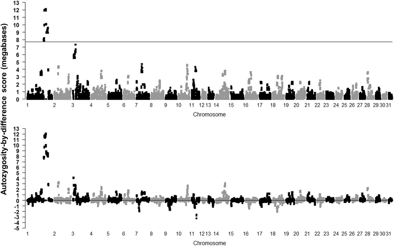
The result of using the novel ABD method is shown in the Supplementary Figure S4 (controls) and Figure 2 (cases and ABD score), with the permuted probability of the difference, after 1000 permutations, being significant for ABD values >4315 kb (P=0.001). The cases in the ABD method pointed to a 1.56-Mb region from base position 136 812 666 to 138 375 254 on ECA1, with the highest ROH score in cases (12.1 Mb), all having P<0.001. These results also highlight the inbred nature of the cases as a number of other ROH were found on various chromosomes which had probabilities <0.05 (ROH in cases >3.6 Mb). Many of these were also found in controls, indicating ‘breed-specific’ ROH (Supplementary Figure S4).
Results of calculating mean runs of homozygosity (ROH) scores for the Lavender Foal Syndrome data set cases using the autozygosity-by-difference method (P=0.05 shown as ROH=3576 kb after 1000 permutations on cases; top plot) and as differences between cases and control mean ROH length (permutated 0.001 P-value shown after 1000 permutations as 4315 Kb; bottom plot) (based on the EquCab2.0 build of the horse genome).
Permutation of the Lavender Foal Syndrome data set
Using the default setting in PLINK with 1 to 500 000 permutations, a series of probabilities were obtained using the genotypic model with the LFS data using the χ 2 genotypic method. These are summarised in Table 4. The number of SNP in the three probability bands appeared to stabilise by about 5000 permutations but the top SNP (i.e. those with the lowest probability) were not always consistent between the runs (data not shown). In fact the top SNP had a genotypic distribution of 5/0/1 and 0/22/8 (AA/AT/TT) for cases and controls respectively; the second SNP was distributed as 0/0/6 and 7/21/2. The top four SNP in all runs were the same as found with the Fisher’s Exact test but were not in the final 1.56 Mb target region containing the LFS variant. These genotypic distributions highlight two points: first significance is gained when both alleles are at an intermediate frequency and, second, PLINK will switch the order of genotypic frequencies by MAF as seen in these results.
Results of running a different number of permutations for the Lavender Foal Syndrome data set using PLINK label-swapping permutation for a genotypic χ Footnote 2 table

SNP=single nucleotide polymorphism; ECA=horse chromosome number.
Discussion of single nucleotide polymorphism-based methods
It is common knowledge that SNP-based methods for finding the site of a new autosomal recessive variant can only locate a target region which is likely to contain the variant, not the variant itself. The mean length of the target regions found from the review of 36 genetic diseases was 4.6 Mb. Thus SNP-based methods are just a preliminary piece of research which needs to be followed up in order to locate the actual variant. (of course, this ignores the extremely unlikely scenario where a SNP is located at the site of the actual variant). The length of the region depends on the recombination events that have occurred either side to the variant’s location since its point of origin in the pedigree. Recombination rates are heritable, arranged in hotspots or random (Fedel-Alon et al., Reference Fledel-Alon, Leffler, Guan, Stephens, Coop and Przeworski2011) and so the length of any given located region will vary depending on how these factors play out in any given species, breed or chromosome involved.
Secondly, SNP-based methods as reviewed here can only map autosomal recessive conditions. They cannot locate dominant conditions, have limited applicability to sex-linked conditions and probably can be used for sex-limited examples in females. Conditions involving more than one gene, traits with age-related onset, environmental ‘triggers’ (probably referred to as having variable expressivity or incomplete penetrance in the older literature) are more challenging. Not surprisingly therefore, when taken in conjunction with the problems of the commonly used methods highlighted above, the published literature represents the ‘low-hanging fruit’ of autosomal recessive conditions and more complicated situations are not easily solvable using these SNP-based methods.
Thirdly, the review of methods summarised in the Supplementary Table S1 highlights the plethora of methods used to located the target region of a new autosomal recessive condition and indicates problems with the readily available packages (PLINK, ASSHOM/ASSIST). The most commonly used method (χ 2) appears to require a second method in order to refine the results, or even replace it, whereas the ASSHOM/ASSIST methods appear to work on their own. Howrigan et al. (Reference Howrigan, Simonson and Keller2011) compared three ROH methods on simulated data (PLINK, BEAGLE and GERMLINE) and recommended the PLINK ROH approach with fine tuning of the parameters to suit the data set involved.
Finally, the basic approach employed to map an autosomal recessive condition using SNP genotypes is to look for characteristic patterns of these conditions in the data derived from cases and controls. In the case of the χ 2 test, and using the genotypic model, this pattern is a significant divergence from the expected distribution of cases and controls between the genotypes, predicated on the marginal numbers of cases, controls and the three genotypes. In the case of a pair of adjacent SNP, one bimorphic for adenine (A) and guanine (G) and the other for cytosine (C) and thymine (T), the new variant may arise between them (the situation where a SNP is actually involved in the variant will be very rare). Although not often stated, the assumption is that there would be a number of highly significant SNP together in the region around the causal variant.
Assuming that the variant is denoted by * and it occurs between the SNP of an AC haplotype, for example, after a few generations the possible haplotypes in the population are A*C, A-C, A-G, T-C and T-G, where - indicates the ‘wild-type’ allele of the variant. Somewhat less likely are A*G and T*C, due to a recombination event between the variant and one SNP, and even less likely is T*G, due to two recombination events, one between the variant and each flanking SNP. Ignoring these recombination possibilities, the likely genotypes in the population are shown in Table 5. In any given population, the number of animals with each genotype will depend on a range of factors. These include the allele frequencies of the two alleles, the recombination rate in that region of the genome, the number of generations since the variant occurred, whether the variant is lethal and the proportion of carriers acting as parents.
Possible genotypes at two adjacent single nucleotide polymorphism (SNP) loci, one polymorphic for adenine (A) and guanine (G) and the other for cytosine (C) and thiamine (T), when a variant (*) occurred between two SNP on the AC haplotype a few generations back

Haplotypes shown vertically; wild-type shown as -. One chromosome of the autosomal pair shown on each axis.
In an autosomal recessive condition, the cell in the top left corner of Table 5 represents an affected individual (case). All other individuals in the top row and leftmost column are carriers and the remaining cells contain non-carriers; both these latter two groups of individuals have a normal phenotype (controls). The χ 2 test cannot distinguish between these different individuals and so may lose its power unless all controls are parents of the cases. In addition, notice that some carriers have the A-A* (or A*A-) genotype and so are indistinguishable from cases when considering this SNP. In a real population these animals, plus the A-A- animals shown in the second and third rows and columns of Table 5, are in a segment of the pedigree which is historically separate from that of the originator of the condition. This is an example of the ‘hidden-SNP problem’ outlined by Stumpf and McVean (Reference Stumpf and McVean2003).
Comparison of methods
Table 1 contains the key results from the five methods compared in this paper. The top row shows the region and base position found by Brooks et al. (Reference Brooks, Gabreski, Miller, Brisbin, Brown, Streeter, Mezey, Cook and Antczak2010) in their original paper. The critical test used here is that any other method should also find this region. If it does, then it is a useful substitute for the two-stage approach used by Brooks et al. (Reference Brooks, Gabreski, Miller, Brisbin, Brown, Streeter, Mezey, Cook and Antczak2010), if not then it has severe limitations. Comparing the 2nd with 7th row in Table 1 shows that only the two ABD-based methods replicated the required results. All other methods highlighted an alternative chromosome (PLINK, ASSIST and ASSHOM) or a much longer region containing the new variant (χ 2 genotypic model).
The reasons for the limitations of the other methods are discussed below but the critical point to stress here is that if these other methods had been used as the sole way to find the new variant then they would not have unequivocally highlighted the position of the LFS variant as being the most likely region.
Table 1 also demonstrates that PLINK, ASSHOM and ASSIST may help to highlight the required region but with some ambiguity. PLINK found the same ‘correct’ region as that with the ‘longest mean length’ and the second highest score of ASSHOM also was in the ‘correct’ region. ASSIST was less effective, finding the region with its second highest region but this included the target region in a 16.0-Mb run, and its longest run did not contain the variant position.
Limitations of the χ 2 test
Although the original analysis of the LFS data set used the genotypic χ 2 test to locate the new variant, the results of using the allelic, dominant and recessive models on these data are shown in the Supplementary Material S2. Any of these methods would have come to a similar conclusion. Table 2 is very informative about the value of the χ 2 test in finding the site of a new autosomal recessive. As noted above, the SNP with the highest χ 2 value was not in the identified region, after haplotype analysis. In addition, the variant was finally found to be between two SNP, one of which was monomorphic and the other would have been except for one control heterozygote. These results call into question the value of the χ 2 test for finding the site of a new variant. Strictly speaking, the SNP either side of the variant should not have been in the analysis because they have a MAF of <0.05. The discussion of the χ 2 test in the Supplementary Material S2 also draws attention to some of its other limitations. These results illustrate the inadequacy of the χ 2 approach in many scenarios and it will only be successful when the allele frequency of the target allele is very low in controls. This may be the ‘unwritten’ assumption about the χ 2 method that the variant segregates with one allele and the wild-type with the other but this is likely to be a minority event. Assuming that a variant is a random occurrence, then it will be associated with a particular SNP allele in proportion to the allele frequency in the population. Hence, the major allele frequencies are likely to be linked to the variant and so more difficult to find using the χ 2 method.
As noted above, the χ 2 method also resulted in very long target regions being found, which were subsequently refined with some sort of ROH method to a much smaller region. This suggests that use of the ROH method initially would have been a better option. What has happened in the LFS data set is that the ROH associated with the variant has been ‘found’ because the alternate allele had a high frequency at SNP in a region of high homozygosity. If the new variant was in a region with completely monomorphic SNP, to take the extreme case, then it would not be found by the χ 2 method. At best, the SNP with intermediate allele frequencies will help to highlight the region with a long ROH.
Homozyg option in PLINK
The use of the –homozyg option in PLINK did locate the target region with the LFS data set but some interpretation of the output was necessary. In a new situation, where the ‘answer’ is not already known, it would be more difficult to arrive at the true location of the target area from among the different regions highlighted. The output is only suitable for visualisation in a Manhattan Plot with specialised software, such as detectRUNS (Biscarini et al., Reference Biscarini, Cozzi, Gaspa and Marras2018), so is more cryptic than other methods and does not allow for any exploratory work into the results to aid interpretation. This was not a drawback with the LFS data set but where there are long ROH which are breed characteristics then the site of the new variant may not be clearly demarcated from these other regions, leading to further ambiguity in the interpretation of the results.
The homozygosity scoring method of Charlier et al. (2008; ASSHOM)
The ASSHOM method of Charlier et al. (Reference Charlier, Coppieters, Rollin, Desmecht, Agerholm, Cambisano, Carta, Dardano, Dive, Fasquelle, Frennet, Hanset, Hubin, Jorgensen, Karim, Kent, Harvey, Pearce, Simon, Tama, Nie, Vandeputte, Lien, Longeri, Fredholm, Harvey and Georges2008) has been widely used to locate a new autosomal recessive condition, as seen in the literature review above. It gives ‘longer and rarer’ haplotypes a higher score. However, there is no reason to expect rarer haplotypes to contain the variant (see Table 2) so it seems illogical to score them higher. Taking the LFS results as an example, the top ASSHOM score on ECA6 was located in a region with no heterozygous SNP genotypes but both a mixture homozygotes at many SNP in cases (results not shown).
The core-marker scoring method of Charlier et al. (2008; ASSIST)
The ASSIST method of Charlier et al. (Reference Charlier, Coppieters, Rollin, Desmecht, Agerholm, Cambisano, Carta, Dardano, Dive, Fasquelle, Frennet, Hanset, Hubin, Jorgensen, Karim, Kent, Harvey, Pearce, Simon, Tama, Nie, Vandeputte, Lien, Longeri, Fredholm, Harvey and Georges2008) has also been widely used in animal studies. Like ASSHOM, the scores for the core marker score higher for rarer alleles in the controls but again there is no reason why this should be true for a new autosomal recessive condition. ASSIST searches for SNP which are monomorphic in cases but polymorphic in controls but, as demonstrated in Table 5, it is possible to have cases and controls which are monomorphic but the cases contain A*A* genotypes and the controls A-A- or A*A-. The top and left hand nine boxes in Table 5 contain SNP homozygous for the AA genotype but only one of the nine will be a case, the other eight are either carriers or non-carriers. Of course the */- nature of the A allele is unknown when genotyping animals using the SNP chip. In addition, the variant in the LFS data set was located between two SNP, one of which was monomorphic in all animals and the other all but monomorphic, but for one control heterozygote. The highest ASSIST core-marker scores found in the LFS data set were not continuous but were interspersed with SNP which were not monomorphic in cases and polymorphic in controls, as stated by the method. The top ASSIST score was an isolated SNP which was monomorphic in cases and polymorphic in controls, surrounded by non-core marker SNP but nevertheless in a long ROH. This also does not resonate with the requirement for the variant to be located between two SNP which are monomorphic in cases, as stated above. Clearly, neither ASSHOM nor ASSIST found the location of the LFS variant as having the highest score but they did highlight the correct region as being a possibility.
Autozygosity by difference method
The ABD method attempts to optimise the calculations necessary to find a new autosomal recessive condition taking into account misgenotyping, misphenotyping, breed-specific ROH, inbreeding, late-age-onset diseases, incomplete penetrance and variable expressivity. Firstly, SNP are only ‘scored’ if they have the same homozygous genotype as that of the cases as this is what is expected in an autosomal recessive condition. Ideally, this would be all cases but in the ABD method this is the homozygous genotype found in the majority of cases. This allows for any misphenotyping or misgenotyping which may have randomly occurred. Secondly, a ROH is constructed for two or more SNP identified in the first step, within each animal (cases and controls) and autosome. Once a heterozygote or a homozygote that is not the commonest at that SNP is encountered the ROH terminates and the length calculated in base pairs, using the midpoint between the first (or last) SNP in the ROH and the previous (or next) SNP. Missing genotypes are scored as if they were the commonest homozygote; this does not penalise misgenotyping. All SNP in the ROH are assigned that length and so are all scored the same within an animal. Thirdly, the mean ROH length at each SNP is calculated in cases and controls separately. In addition, their difference is calculated at each SNP. This removes the effect of any breed/population-specific ROH from the calculations and should leave the largest values as containing the new variant, as a long ROH found in cases, but not controls, is required. Finally, phenotypes (case or control) are randomly assigned to the animals and the calculations rerun, say 1000 times, and the results stored along with those from the ‘true’ original phenotypes. Significance is calculated as the proportion of the results higher than a given value. This may be carried out for cases alone, or the ABD scores as required using an option in the ABD software, resulting in permuted probabilities for either score (mean case ROH or ABD). This helps to account for inbreeding as, without the new variant ROH, one would expect a random distribution of high scores across the individual genome to the same degree in both cases and controls. Inbreeding is accounted for since longer ROH are also a result of inbreeding and are present at similar levels on all chromosomes of any given animal. By including all ROH in the permutations, the significance of the ROH due to the new variant is estimated over and above that of the level of inbreeding of each animal. Incomplete penetrance or a late-onset disease both result in cases containing long ROH but also some controls may have the same genotypes as well, either because the variant has been prevented from expressing itself due to environmental or other gene influences (incomplete penetrance; e.g. Drogemuller et al., Reference Drogemuller, Jagannathan, Welle, Graubner, Straub, Gerber, Burger, Signer-Hasler, Poncet, Klopfenstein, von Niederhäusern, Tetens, Thaller, Rieder, Drögemüller and Leeb2014) or because the animal has not reached its age-trigger (late onset condition; e.g. Kyostila et al., Reference Kyöstilä, Syrjä, Jagannathan, Chandrasekar, Jokinen, Seppälä, Becker, Drögemüller, Dietschi, Drögemüller, Lang, Steffen, Rohdin, Jäderlund, Lappalainen, Hahn, Wohlsein, Baumgärtner, Henke, Oevermann, Kere, Lohi and Leeb2015). In this situation, the ABD method will still score the cases highly but the controls will also have an inflated score due to the ‘hidden’ ROH’. This can be seen through inspection of the individual animal scores in a suitable program, for example a spreadsheet. One of the outputs from the ABD method is a file of SNP by animals showing the ROH scores for each animals at each SNP. This file allows the investigation of the any region of interest, for example similar long ROH in controls to the target region in cases as an indication of incomplete penetrance or a late-onset condition.
Use of the ABD method was demonstrated to ‘find’ the ROH containing the new variant causing the LFS in a 1.56-Mb length of ECA1. The area of ECA1 containing target region achieved significance at P<0.001 after 10 000 label-swapping permutations of the ABD score, and was the only area to do so throughout the genome. It could be considered the most useful method as it located the target area of Brooks et al. (Reference Brooks, Gabreski, Miller, Brisbin, Brown, Streeter, Mezey, Cook and Antczak2010) in one step, with very low probability and without ambiguity. No other method tested demonstrated all three characteristics. In conclusion, it would seem best to avoid the use of the χ 2 method and use the ABD method as the initial step on as many cases as possible and a similar number of controls.
Final step methodology
Using whole genome sequencing data
The papers reviewed in this study all used a three-stage approach as a minimum to locate a novel autosomal recessive variant and none of them used WGS data at the first stage. Once a target region had been identified by two stages, 11 of the reviewed papers followed this up with WGS data to help locate the causal variant.
One of the differences between using SNP array and WGS data is that, with WGS data, it should be possible to find a base position with the appropriate pattern of genotypes (genotype criteria) for the data set being studied, assuming perfect sequencing by whichever method is used. Thus if using a data set with six cases and six parents as controls, then the genotype criteria would be a base position with all six cases homozygous for the same base (or insertion/deletion; indel) and the six parents would be heterozygous for this base (or indel) and another base (or indel). Alternative scenarios would be to use no controls or any number of ‘unrelated’ controls. In the former example, the genotype criteria would be homozygous for the same base at one base position and in the latter example the controls would be a mixture of heterozygotes and homozygotes comprising a base (or bases) not found in the cases. At first sight, looking for such a base position might appear a daunting task in a typical mammalian genome of 3 billion bases. However, there are a number of ways to cut down the search. First, the large majority of base positions are monomorphic (Szyda et al., Reference Szyda, Fraszczak, Mielczarek, Giannico, Minozzi, Nicolazzi, Kaminski and Wojdak-Maksymiec2015) and so can be ignored, reducing the task down to searching among base positions which are polymorphic. Second, WGS data should provide ‘exact’ information on ROH in the cases and controls. A suitable program could be used to reduce the search area down to the target region with the longest mean ROH in cases, taking into account any ROH which are breed specific (e.g. ABD). The task might, therefore, be reduced to looking for the genotype criteria in cases and controls (or cases alone) at polymorphic sites within a relatively short stretch of one chromosome.
Size of sample to sequence
Taking the bovine genome to be 3 billion base positions long with 15 million single nucleotide variants (SNV), in a breed such as the Holstein (Szyda et al., Reference Szyda, Fraszczak, Mielczarek, Giannico, Minozzi, Nicolazzi, Kaminski and Wojdak-Maksymiec2015), and taking a target region of 2 Mb, it is possible to calculate how many base positions would have the genotype criteria in cases and controls for a range of experiment sizes. At any bimorphic base position, there would be three possible genotypes (say AA, AT and TT). The chance of getting the same homozygous genotype (AA) in all n cases would be 1/3 n . It would be the same for m parental controls and in fact for the total sequenced population of n+m; 1/3 n+m . The same calculation would apply if only cases were used. The only different result would be when the m controls were a random selection of the breed; in this event, the probability would be 2/3 m for controls as they could have either the AT or TT genotypes at the variant site. Figure 3 shows the number of base positions that would be found to have the genotype criteria for the four different scenarios: whole genome, all SNV, a 2-Mb target region and the SNV within the target region. This can be used to estimate the number of animals that would need to be genotyped in order to find the variant as the only base position fulfilling the genotype criteria. This turns out to be 20 animals for the whole genome, 16 for all the SNV, 14 for the 2 Mb region and 11 for the SNV within that region. This would be the estimate for the three situations of genotyping: (1) only cases, (2) case plus one parent or (3) trios of cases and both parents. The only difference is that the number of required cases would be increasingly reduced from 20 to 10 to 7, respectively, for the three situations using whole genome data. In the example of one unrelated control for each case the results are only marginally greater, for example 21 animals required in total for the whole genome results. In reality some base positions are likely to be more than bimorphic, could be at the site of an insertion or deletion, and the actual variant site in controls will not contain the homozygote found in the cases but none of these alter the conclusions reached above to any practical extent.
The number of base positions likely to be found with the appropriate genotype criteria when two to 21 animals are whole genome sequenced for four scenarios: complete genome data (3 billion bases; whole genome), all single nucleotide variants (15 million SNV; all variants), all bases in a 2 megabase (Mb) target region (2 Mb target region) and all SNV in target region (2 Mb target region variants).

In an attempt to see if these theoretical calculations were borne out in practice, the 11 reviewed papers that used WGS were scanned to see if there was any supporting data. Bauer et al. (Reference Bauer, Hiemesch, Jagannathan, Neuditschko, Bachmann, Rieder, Mikko, Penedo, Tarasova, Vitková, Sirtori, Roccabianca, Leeb and Welle2017) used two cases, two carriers and 75 horses from other breeds, and found five SNV in a 17 Mb target region using a criterion that included homozygous reference genotypes in the ‘other breed’ animals. Finno et al. (Reference Finno, Stevens, Young, Affolter, Joshi, Ramsay and Bannasch2015) sequenced two cases and two controls and looked in a 1.74-Mb target region which contained 363 SNV of the appropriate pattern. Venhoranta et al. (Reference Venhoranta, Pausch, Flisikowski, Wurmser, Taponen, Rautala, Kind, Schnieke, Fries, Lohi and Andersson2014) used a single case, one parent and resequenced further 43 animals in the target area. They found four SNV in a 0.7-Mb region and went on to eliminate three of them using the 1000 bull genome data. Finally, Jung et al. (Reference Jung, Pausch, Langenmayer, Schwarzenbacher, Majzoub-Altweck, Gollnick and Fries2014) sequenced one case, one parent and 41 unrelated animals and found four SNV in a target area of 1.02 Kb. It is not always clear from these reports how the status of the control animals was used to define a likely SNV as being the new variant. However, evidence does point to a small number of SNV being found within a previously defined target area which may be confirmed using controls from other sources.
Methodology to find the variant using whole genome sequencing
The approach to finding the variant site using WGS data described above can be achieved using the commonly found variant call format (VCF) file produced by WGS software such as SAMTOOLS or GATK from whole genome sequences aligned to the reference genome. This file can be scanned for evenly spaced bimorphic SNV for use in a suitable program, such as ABD described above, to locate the target region. This should produce a target region in which to search for the appropriate genotype criteria. The variant may not be a single base change but an insertion or deletion. These are still denoted in the VCF file and can still be recognised in heterozygote carriers.
The most common method for finding the causal variant of a new autosomal recessive condition among the 11 reviewed papers using WGS data involved sequencing a small number of cases. In some instances, these data were used in conjunction with previously sequenced animals of other breeds as controls to find likely sites, as outlined above. Where several SNV were found, then biological function was often used to refine the number down. This often involved looking at functional changes in genes caused by the various SNV. Several papers used the 1000 bull genomes data as controls, looking for sites that were completely homozygous for the reference allele. All papers used the previously located target regions in which to search. Some papers confirmed their results by genotyping other samples at highlighted locations.
Using whole genome sequencing data in the future
Given the calculations above and the methodology used by the reviewed authors suggests a good strategy for finding the location of a new autosomal recessive variant. Clearly, a small number of cases need to be sequenced so that the novel piece of sequence caused by the variant can be identified. Sequencing enough controls to leave only one site as having the required unique combination of genotypes appears to require just over 15 animals in total in the case of cattle with ~15 million SNV in a VCF file. As several authors have already noted, use of the 1000 bull genomes project SNV and indel data can be substituted for controls in the case of new cattle diseases and so the number of newly genotyped animals would reduce to about three cases, just to highlight the new sequence caused by the variant. Clearly, similar resources are required to be available for other species. If this were the case, then the cost of finding the site of a new autosomal recessive variant would be the cost of whole genome sequencing a few cases plus the necessary bioinformatic resources to assemble to necessary data and run a program over the VCF-type data.
A possible future analysis
∙ Sequence the whole genomes of about five cases and 10 controls.
∙ Search the SNV in a VCF file for the base positions with the correct genotype criteria.
OR
∙ Sequence three cases and six controls.
∙ Run ABD on suitably selected SNP to find target region.
∙ Search for SNV with the correct genotype criteria in the target region.
OR
∙ Sequence three cases.
∙ Use resource files (1000 bull genomes data or similar) as controls.
∙ Search for SNV with the correct genotype criteria.
If SNP genotypes are available, then it would be better to find the target region before whole genome sequencing a sample of cases and controls using a ROH method like ABD. Depending on the size of the target region found, it might only need about six animals to be whole genome sequenced.
Conclusions
The problem of finding the site of a new autosomal recessive variant has proved to be difficult over recent years in those cases where homology to a known condition in other species is not possible. A variety of methods have been tried which says much for the ingenuity of the animal science research community as well as the apparent intractability of the problem. No single solution appears to have been taken up widely. It appears that several authors have struggled with the apparently simple and straightforward approach (χ 2). The probable reasons for this have been explored in this review, which highlighted the fact that the χ 2 methods was almost never used on its own and was nearly always followed up by one of a range of methods. The other commonly found methods have all been found to have some flaws which have been addressed in the ABD method suggested in this paper. Another feature of all the reviewed reports of successful searches highlight the fact that the procedure always involves more than one stage; an initial analysis using SNP to locate a target region and then an exploration of this target region either by resequencing candidate genes or WGS and then searching for an appropriate pattern of genotypes in cases and controls at the base position level. Based on the experience of the authors of reviewed papers, it is suggested here that future approaches should whole genome sequence about 15 animals comprising between three and six cases, and then search the VCF files for sites with appropriate combinations of genotypes. This approach will become cheaper and easier to achieve as sequencing costs decline and bioinformatic methods become more widely available in the near future. If suitable data are available from unrelated animals of the same species, then these could be used as controls and hence reduce the number of animals that need to be sequenced. Alternatively it may be possible to use sequence data to define the target area using about 10 sequenced animals in conjunction with the ABD method, and search within that area for the SNV of interest.
Acknowledgements
Doug Antczak and the team at Cornell University are gratefully acknowledged for providing the Lavender Foal Syndrome data analysed in this paper.
Declaration of interest
There is no conflict of interest involved with this paper.
Ethics statement
This paper is a review and analysis of previously published data. No new ethical approval was required.
Software and data repository sources
No new data was generated in this paper.
Supplementary material
To view supplementary material for this article, please visit https://doi.org/10.1017/S1751731118001970


 Open access