1. Introduction

Near-surface temperature, Ta, typically measured at a height of 2 m, is the most important control on the energy exchange and melt rate at a snow or ice surface in many glacier melt models. For spatially distributed glacier melt modelling, a distributed temperature input is needed, which is normally generated by extrapolation from point measurements with a linear lapse rate (LR). The LR describes the dependency of temperature on elevation and is considered to be positive when temperature increases with elevation (e.g. Reference Minder, Mote and LundquistMinder and others, 2010). A steep (strongly negative) LR indicates a fast decrease in temperature with increasing altitude (see, e.g., Reference Pepin and LoslebenPepin and Losleben, 2002). In most glacier melt models, the temperature is represented with a LR that is constant in time and uniform in space (e.g. Reference Klok and OerlemansKlok and Oerlemans, 2002; Reference Hock and HolmgrenHock and Holmgren, 2005; Reference Machguth, Paul, Hoelzle and HaeberliMachguth and others, 2006; Reference Huss, Bauder and Funk Mand HockHuss and others, 2008; Reference Farinotti, Usselmann, Huss, Bauder and FunkFarinotti and others, 2012). Generally such a LR lies between -0.0055 and -0.00658Cmr1 (e.g. Reference Arnold, Rees, Hodson and KohlerArnold and others, 2006; Reference Machguth, Paul, Hoelzle and HaeberliMachguth and others, 2006; Reference MichlmayrMichlmayr and others, 2008; Reference Gardner and SharpGardner and Sharp, 2009; Reference Paul, Escher-Vetter and MachguthPaul and others, 2009; Reference Nolin, Phillippe, Jefferson and LewisNolin and others, 2010), the latter often being referred to as the environmental lapse rate (ELR) (or mean moist adiabatic lapse rate (MALR)). Both the assumption of a LR that is constant in time and uniform in space and the use of the ELR have recently been questioned for high-elevation and glacierized basins. Most studies on the variability of near-surface temperature LRs over glaciers have found generally lower LRs than those commonly used (e.g. Reference Strasser, Corripio, Pellicciotti, Burlando, Brock and FunkStrasser and others, 2004; Reference Li and WilliamsLi and Williams, 2008; Reference Hulth, Rolstad, Trondsen and Wedoe RodbyHulth and others, 2010), while Reference Minder, Mote and LundquistMinder and others (2010) pointed out that there is no physical basis for the use of the ELR in high-elevation basins where the effect of the terrain cannot be neglected. Spatio-temporal patterns of air temperature variability have been shown to be affected by various factors of the surface environment and atmospheric conditions (see Reference Marshall, Sharp, Burgess and AnslowMarshall and others, 2007), so that the application of free-atmosphere LRs is questionable. Temporal variability has been shown to be important at all scales in various studies (e.g. Reference Stahl, Moore, Floyer, Asplin and McKendryStahl and others, 2006; Reference Marshall, Sharp, Burgess and AnslowMarshall and others, 2007; Reference Chutko and LamoureuxChutko and Lamoureux, 2009; Reference GardnerGardner and others, 2009; Reference Petersen and PellicciottiPetersen and Pellicciotti, 2011), while spatial variations are more complex than the simple linear dependency with elevation assumes (e.g. Reference Strasser, Corripio, Pellicciotti, Burlando, Brock and FunkStrasser and others, 2004; Reference Brock, Mihalcea, Kirkbride, Diolaiuti, Cutler and SmiragliaBrock and others, 2010; Reference Petersen and PellicciottiPetersen and Pellicciotti, 2011). An additional limitation of the use of a constant LR to extrapolate air temperature from off-glacier stations is that changes in temperature are generally higher off-glacier than on-glacier because of the damping effect of the glacier (Reference Greuell and BöhmGreuell and Böhm, 1998). Because of the presence of a surface at its melting point and the katabatic wind, the 2 m temperature of the air above the glacier is intermediate between the temperature in the free atmosphere and the fixed temperature of the surface (glacier damping effect). As a result, changes in 2 m temperature will be smaller than those in the corresponding free atmosphere, what has been referred to as a reduced sensitivity to climatic changes (Reference Greuell and BöhmGreuell and Böhm, 1998). This effect cannot be taken into account using a simple LR, and the higher temperature changes would be translated as such onto the glacier surface, resulting in overestimation of melt rates. Depending on the type of melt model used, however, on-glacier temperatures have sometimes been found to lead to worse model performance compared with extrapolations based on off-glacier temperature measurements (Reference Gumundsson, Björnsson, Palsson and HaraldssonGudmundsson and others, 2009), indicating that the damping effect of the glacier may obscure the relationship between atmospheric temperatures and glacier melting.

Lack of extensive Ta datasets on glaciers is a key constraint on a thorough analysis of temperature variability in space and time, as well as on the development of models. Using a high-resolution dataset of temperature time series at several locations along the flowline of Glaciar Juncal Norte, Chile, Reference Petersen and PellicciottiPetersen and Pellicciotti (2011) found a strong diurnal LR cycle driven by the development of a katabatic boundary layer (KBL), with steeper LRs in the afternoon when katabatic wind was eroded and elevation was re-established as the main control on air temperature variability. A KBL develops on melting glaciers when the air temperature above the glacier, which is normally higher than that of the glacier surface (which cannot exceed 08C), is cooled by the surface. The cooling increases its density, and the resulting density gradient produces katabatic flow (e.g. Reference OhataOhata, 1989; Reference Greuell, Knap and SmeetsGreuell and others, 1997; Reference Klok, Nolan and Van den BroekeKlok and others, 2005; Reference PellicciottiPellicciotti and others, 2008). Most studies using procedures to generate temperature fields to drive melt models do not account for processes within the KBL (Reference Shea and MooreShea and Moore, 2010) even though it is a main control over temperature variability. The presence of the KBL affects the thermal regime by reinforcing the turbulent exchange of heat by sensible fluxes and the cooling of the air adjacent to the surface. As a result, temperatures are lower within the KBL than outside (Reference Greuell and BöhmGreuell and Böhm, 1998; Reference Marshall, Sharp, Burgess and AnslowMarshall and others, 2007; Reference Shea and MooreShea and Moore, 2010). Empirical approaches to take into account the difference in regime between on- and off-glacier temperature have been suggested by Reference Braithwaite, Zhang and RaperBraithwaite and others (2002) and Reference Shea and MooreShea and Moore (2010). An attempt to include these effects was proposed by Reference Greuell and BöhmGreuell and Böhm (1998) with a thermodynamic model (henceforth referred to as GB98) in which air temperature is derived as a function of slope and distance along the flowline. This approach was suggested because air temperature variations along Pasterze glacier, a valley glacier in Austria, could not be explained using a constant LR (see Section 4). GB98 is, to our knowledge, the only model of air temperature distribution on glaciers that has been suggested as a realistic and practical alternative to extrapolation using LRs. However, there has been little published work applying the model to other glaciers or testing its main assumptions. The aim of this paper is therefore to investigate the suitability of the GB98 model for calculating air temperature distribution across a well-studied alpine glacier, Haut Glacier d’Arolla (HGdA; Fig. 1), Swiss Alps, and to explore its strengths and limitations in comparison with the commonly used LR approach. For this, we use a new dataset of distributed temperature records collected on HGdA during the 2010 ablation season.

Fig. 1.

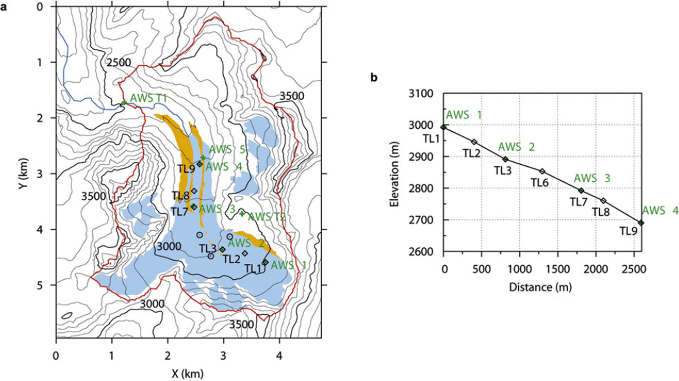
(a) Map of Haut Glacier d’Arolla showing the glacierized area (blue), the debris-covered area (brown) and the catchment outline (red). Green ‘+’ indicates the locations of AWSs in 2010, ‘o’ indicates the positions of T-loggers which are not used in the analysis; the T-loggers along the flowline are indicated with diamonds and labelled. The upper left corner of the plot is 604030, 94910 in Swiss coordinates. (b) Surface profile along the flowline. AWS5 is approximately at the same elevation as AWS4.

2. Experimental Set-Up

Our study site is HGdA, in the Val d’Herens, southern Switzerland (Fig. 1a). It has an area of 4 km2 and a length of 4 km and comprises two basins feeding a tongue. The elevation ranges from 2590 to ∼3500m, with a generally constant and gentle slope (Fig. 1b). About 36% of the basin is glacierized. Numerous studies of glacier energy balance and ablation, meteorology and hydrology have been conducted on the glacier (e.g. Reference Arnold, Willis, Sharp, Richards and LawsonArnold and others, 1996; Reference Nienow, Sharp and WillisNienow and others, 1996; Reference Willis, Arnold and BrockWillis and others, 2002; Reference Pellicciotti, Brock, Strasser, Burlando, Funk and CorripioPellicciotti and others, 2005; Reference Brock, Willis and SharpBrock and others, 2006; Reference Carenzo, Pellicciotti, Rimkus and BurlandoCarenzo and others, 2009).

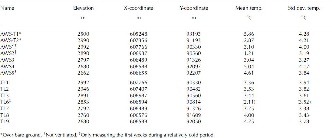
In 2010, a glacio-meteorological field campaign was conducted from 24 May until 12 September. The set-up included the five automatic weather stations (AWSs) and seven T-loggers used in this study (Fig. 1a). The AWSs measured at a 5 s interval and stored averaged 5 min records of air temperature (°C), relative humidity (%), wind speed (ms∼1), wind direction (°) and incoming and reflected shortwave radiation (Wm T 2 ) . The thermometers of AWS2, AWS3 and AWS4 were ventilated and shielded, while AWS1 and AWS5 were shielded but not ventilated. The T-loggers consisted of a HOBO TidbiT v2 UTBI-001 temperature sensor with integrated data logger housed in a shielded PVC cylinder and fixed to a metal tripod 2 m above the surface. The details of this set-up are described by Reference Petersen and PellicciottiPetersen and Pellicciotti (2011). The T-loggers used in this study were located along the glacier flowline, some of them close to the AWSs (Fig. 1a). They measured at an interval of 5 or 10 min. All data were aggregated to hourly values for the analysis. The characteristics of the AWSs and T-loggers are listed in Table 1. We mainly use the temperature data from the T-loggers for the analysis of the temporal and spatial variability of 2 m air temperature and testing of the model, and the data from the AWSs for analysis of wind direction and derivation of cloud transmittance factors. We also use data measured at two permanent off-glacier stations, AWS-T1 and AWS-T2 (Fig. 1a). AWS-T1 is located on rock near the glacier terminus at an elevation of 2500 m. AWS-T2 is set up on periglacial debris of the easterly slopes next to the glacier at an elevation of 2990 m. Longwave radiation (Wmr2 ) and temperature (8C) from the two off-glacier AWSs are used for the calculation of cloud cover and the corresponding determination of cloud classes (Section 5). The temperature record of AWS-T2 provides the input to the model. Some of the T-loggers fell down on the glacier surface during certain periods which were therefore excluded. For the analysis we use only the data when all T-loggers were functioning, so the dataset consists of 1284 hours of non-continuous measurements. TL6 was not considered in the analysis due to a very short functioning period. This common period (grey bar in Fig. 4) is used to compute the main statistics for the temperature series at each T-logger (Table 1). An airborne lidar flight over the HGdA glacier basin in October 2010 by Helimap System SA provided a digital elevation model (DEM) with a grid resolution of 10 m, which is used as the basis of the model in this paper, in particular to derive the glacier slope and the distance along the flowline (Fig. 1). The elevations of the AWSs and T-loggers were measured with differential GPS.

Table 1.

Characteristics of the AWSs and T-loggers: name, elevation, X-coordinate, Y-coordinate, mean temperature and standard deviation. Mean temperature and standard deviation are calculated over the common period of record (1284 hours) unless stated otherwise. The elevation and coordinates of the AWSs and T-loggers were measured with a differential GPS

3. Application of a Constant Lapse Rate (CLR)

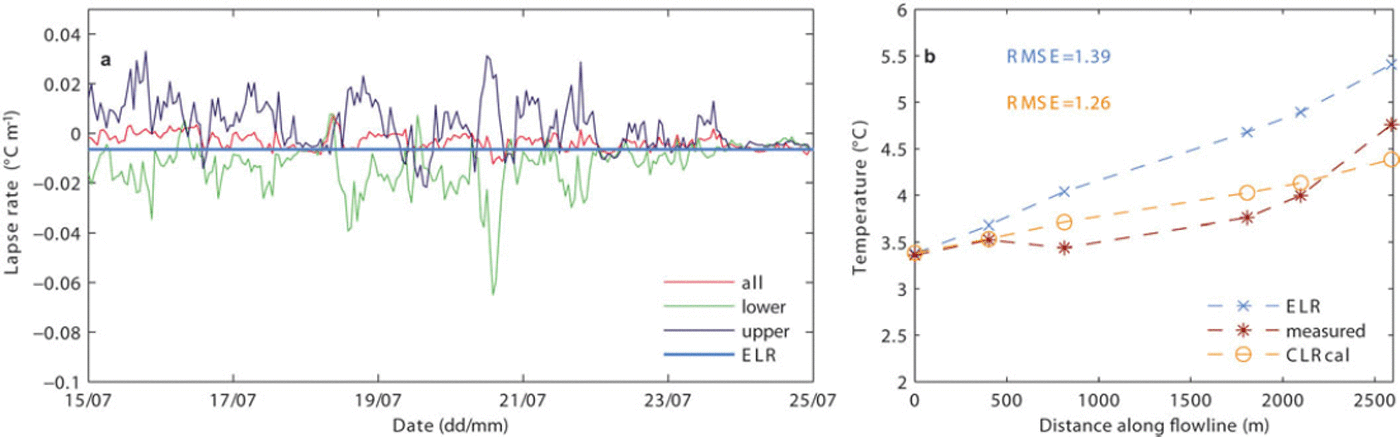
We calculated a LR that was constant in time and uniform in space, using the data from the T-loggers, as well as a LR variable in time, to test the validity of the commonly used method of Ta extrapolation on HGdA. The data show high temporal variability on different scales, as well as spatial variations across the glacier (Fig. 2a). The figure shows the lapse rate calculated through linear regression using (1) all T-loggers, (2) all T-loggers in the lower part of the glacier (TL7, TL8, TL9) and (3) all T-loggers in the upper part (TL1, TL2, TL3). Differences in LR between the upper and lower sections and over the season are significant. The lower section of the glacier is characterized by steep, negative LRs, while the upper section has less negative LRs or even positive ones, indicating inversions. Use of a single variable LR for the entire glacier averages out the two behaviours and reduces the observed temporal variability. If the LR is also averaged in time over the season, we obtain an unrealistic value that only results from compensation of contrasting patterns. It is thus evident that application of a constant LR will not represent the actual temperature variability over the glacier, in time or space. Figure 2b shows the comparison of observed temperature with temperature extrapolated from AWS-T2 with the ELR (-0.00658Cmr1) and a calibrated constant LR (CLRcal). Prior to the extrapolation, data at AWS-T2 were corrected. A systematic difference between the temperature data at AWS-T2 and at the uppermost T-logger, TL1, is evident (Table 2). Although the two stations are at almost the same elevation, the mean temperature over the common period is ∼0.58C lower at AWS-T2 than at the location on the glacier (Table 2). This might be because the location of AWS-T2 is windier and the air is better mixed. It could also be due to differences in the ventilation of the sensors as well as the fact that the boundary layer at TL1 might be thin and thus the station might measure outside the GBL. However, the exact cause cannot be identified precisely, given the limited number of data available. To exclude this systematic error, we corrected the temperature at AWS-T2 with an offset of 0.58C. The constant LR was calibrated by minimizing the root-mean-square error (RMSE) at all T-logger locations over the whole time series for the common period of record. The CLRcal is equal to -0.00328C m r 1 and thus shallower than the ELR, confirming evidence from previous studies (e.g. Reference Marshall and SharpMarshall and Sharp, 2009; Reference Shea and MooreShea and Moore, 2010). Use of an ad hoc calibrated LR provides an obvious improvement over use of the standard ELR (Fig. 2b).

Fig. 2.

(a) Comparison of the constant ELR with LRs variable in space and time: regression of all T-loggers along the flowline (TL1, TL2, TL3, TL7, TL8, TL9) (indicated by ’all’); upper LR (’upper’) obtained from regression of the upper T-loggers (TL1–TL3); and lower LR (’lower’) obtained from regression of the lower T-loggers (TL7–TL9). (b) Comparison of mean observed temperature at each T-logger with temperature extrapolated from AWS-T2 with the ELR and the calibrated constant LR (CLRcal). Also indicated is the root-mean-square error (RMSE) for the two model versions.

Table 2.

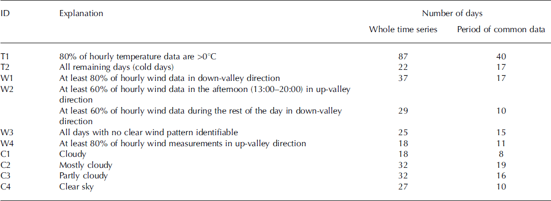
Summary of the climatic categories identified for analysis of the model results, description of criteria and the number of days corresponding to each category

4. Application of the Greuell and Böhm Model (GB98)

In the description of the GB98 model, we follow the notation of the original paper. The main assumption of this simple thermodynamic model is that temperature distribution over a melting glacier is a balance between adiabatic warming (cooling) due to compression (expansion) of air moving along the glacier and the sensible heat exchange with the underlying ice surface (see Reference Van den BroekeVan den Broeke, 1997). Hence, air temperature distribution is parameterized mainly as a function of slope and along-glacier distance. Temperature changes due to surrounding topography, entrainment, phase changes, radiation divergence and variation of fluxes in the horizontal direction are neglected. These assumptions were based on results obtained by Reference Van den BroekeVan den Broeke (1997) on Pasterze glacier during summer 1994. The author argued from analysis of wind directions that conditions on Pasterze glacier were dominated by the katabatic or glacier wind. The model is based on a number of other simplifying assumptions, such as that the height of the glacier wind layer, H, and the glacier slope are constant. These assumptions were discussed by Reference Greuell and BöhmGreuell and Böhm (1998) for Pasterze glacier and are addressed in Section 5. Since the model is based on the hypothesis that the glacier wind is present, a requirement for its application is an air temperature greater than the surface temperature so that the glacier wind is likely to develop (see Section 1).

For the application of the model, the glacier geometry must be known in order to derive slope angle and distance along the glacier flowline. This information can be extracted from glacier DEMs that can also be provided by downloadable global databases (e.g. glacier outlines from the World Glacier Monitoring Service/Global Land Ice Measurements from Space (WGMS/GLIMS) and DEMs from the Shuttle Radar Topography Mission (SRTM)), which makes the model appealing in terms of applicability. We used the DEM described in Section 2. Here we report only the main equations of the model and refer the reader to the original paper by Reference Greuell and BöhmGreuell and Böhm (1998) for more details. The potential temperature 6 is calculated as

From this, the actual temperature can be derived as

with

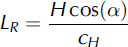
where T(x) is the temperature at a distance x along the glacier flowline, T0 the temperature at x = 0, Teq the equilibrium temperature value, T the dry adiabatic LR (-0.00988Cmr1), cH the bulk transfer coefficient for heat (see Reference StullStull, 1988) and Tcs and zcs are the temperature and elevation of the climate station outside of the glacier’s influence used to drive the model (AWS-T2 in our study). All the equations above are based on the assumptions that the glacier slope is constant and that the ratio H/cH is constant along the flowline.

The equations above contain five unknown parameters: x0 and z0, the location and elevation where the air parcel enters the layer influenced by the glacier; the length scale LR and b (which are defined above and depend on the glacier slope, a); and 7, the lapse rate used to extrapolate temperature from the input climate station, Tcs, to the initial point (x0, z0). Here we apply the model to the entire dataset of temperature observations (common period of record), following the same approach as Reference Greuell and BöhmGreuell and Böhm (1998). We use the same values of 7 (-0.0078Cmr1), H (equal to 17 m as estimated for Pasterze glacier by Reference Greuell and BöhmGreuell and Böhm, 1998) and cH (0.002 following Reference StullStull, 1988) as used by those authors. We refer to this set-up as the unmodified model, but test different assumptions for the position and elevation of the uppermost point of the flowline (x0 and z0), as recommended by Reference Greuell and BöhmGreuell and Böhm (1998), who pointed to the fact that both x 0 and z 0 could be regarded as tuning parameters. The best fit is obtained by assuming the uppermost T-logger (TL1) as the initial point (of coordinate x0 and elevation z0, respectively). Model sensitivity was then analysed by varying the other parameters by ±10, 25 and 50% around the initial values taken from Reference Greuell and BöhmGreuell and Böhm (1998). Variations in H (constant along the flowline), the slope (and thus b and LR) and 7 in the range above resulted in small changes in the temperature profile (not shown here). Varying 7 (±10, 25 and 50%) did not have a major effect, as expected considering the similar elevation of the climate station and of the initial point (TL1) (see Table 1). We also tested the effect of using different off-glacier data as input to the model, but the differences when using the nearest MeteoSwiss station, Grand St Bernard (2472 m, 579137/ 79 856 m, located at a distance of 30.4 km), were negligible.

Figure 3a shows the comparison of measured air temperature with air temperature extrapolated with the calibrated constant LR (CLRcal) and modelled with the GB98 model, for the common period of record. Even though the CLRcal seems to work acceptably, the RMSE is reduced by 7% by applying the GB98. The CLRcal leads to underestimation of temperatures during cold periods and overestimation during warm periods (Fig. 3b). As these two errors compensate each other, the net effect is an apparently good performance if we look only at the average values over the season (Fig. 3a).

Fig. 3.

Comparison of observed temperature and temperature modelled with GB98, with the values of H, 7 and T suggested in the original paper for Pasterze glacier (GB98, i.e. unmodified model) and the modified version (GBvarH, Section 5): (a) average values along the flowline; and (b) time series at TL7 for a selected sub-period (21-27 July).

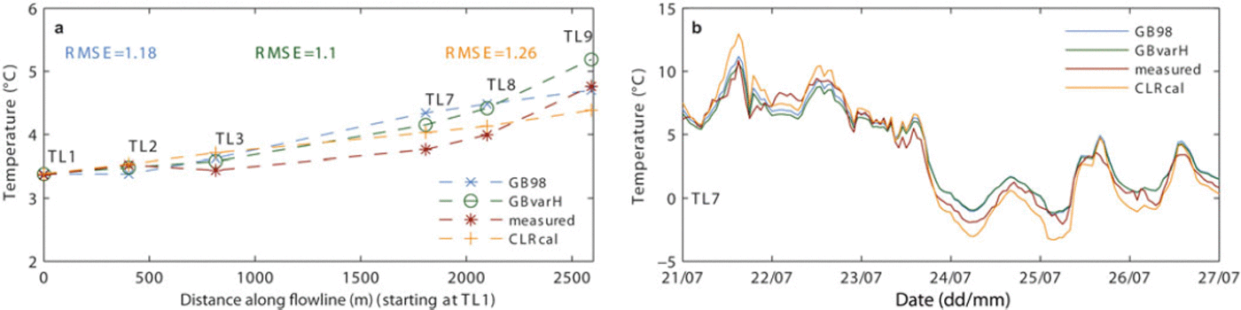
The GB98 on average overestimates temperature in the central part of the glacier (TL3, TL7 and TL8). The observations reveal a profile along the glacier flowline that is characterized by average temperatures decreasing more slowly in the central part of the glacier than in the uppermost and lower sections (Fig. 3b). This profile cannot be reproduced by the model, which exhibits a more linear change in air temperature with distance along the flowline than is observed.

5. Applicability of the GB98 Model under Different Meteorological Conditions

The results of the application of the GB98 model to the entire dataset reveal that the model cannot reproduce the observed variability on HGdA in its original form (Fig. 3), even if parameters are varied to adjust the model outputs to the observations.

The model is based on the assumption of two main fluxes controlling the exchange of energy at the glacier surface and affecting the temperature of air in the GBL (see Section 4), and it requires, in particular, that the glacier wind is well developed. The latter is generated by the temperature deficit between the glacier surface and overlying air, which causes the air particles above the surface to cool and gravitationally flow because of the associated increase in density (e.g. Reference Stenning, Banfield and YoungStenning and others, 1981; Reference Van den BroekeVan den Broeke, 1997; Reference Greuell and BöhmGreuell and Böhm, 1998). We therefore analysed the climatic

1. 1. Temperature: The temperature record was divided into two classes representing low and high air temperature: (i) T1, days for which >80% of the hourly values are >08C; and (ii) T2, comprising the remaining cases. Most days fell into category T1, indicating the existence of conditions favouring the development of katabatic wind.

2. 2. Wind: The influence of wind was investigated by defining four classes: (i) W1, characterized by mainly down-valley wind (>80% of the hourly values); (ii) W2, characterized by a diurnal cycle with mainly down-valley wind at night and in the morning hours (>60% of the hourly values between 21:00 and 12:00) and mainly up-valley wind in the afternoon hours (>60% of the hourly values between 13:00 and 20:00), which was identified as the typical pattern on several days, so that a clear distinction from other conditions could be made; (iii) W3, with a mixed wind pattern (all remaining cases after identifying W1, W2 and W4); and (iv) W4, with mainly up-valley wind (>80% of the hourly values). For this classification, we used the frequency distribution of the wind direction data from AWS4. However, the classification was compared to that obtained from the records at the other AWSs, showing a nearly perfect correspondence.

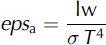
3. 3. Cloud cover: the categories for clouds were derived by classifying the days on the basis of cloud transmittance factors or cloud cover, n, derived from the measured incoming longwave radiation data at three AWSs (AWS-T1, AWS-T2 and AWS5). We adopted the approach of Reference Marty and PhiliponaMarty and Philipona (2000), which is based on the comparison of the atmospheric emissivity epsp and the potential clear-sky atmospheric emissivity epscsp (calculated with the Brutsaert formula (Reference BrutsaertBrutsaert, 1975), for the reasons explained by Reference Marty and PhiliponaMarty and Philipona (2000)). The ratio of the two emissivities provides a clear-sky index, the complement of which is the cloud factor. This method was found to be superior to methods based on the ratio of potential clear-sky to measured shortwave radiation (which are often used (Reference Brock and ArnoldBrock and Arnold, 2000)). The cloud cover was estimated on the basis of a linear regression between epsp and 1, where epsa = epsp corresponds to a cloud cover of zero and epsa = 1 to a cloud-cover of one. The atmospheric clear-sky emissivity is calculated as

   (7)

   

   with T (K) being the air temperature, lw (Wm∼2 ) the measured incoming longwave radiation and ertheStefan-Boltzmann constant. The daily cloud cover n was calculated as the mean of the hourly values at the three AWSs. This value was then used to identify four categories: (i) C1: n > 0:8 overcast days; (ii) C2: 0:4 < n < 0:8 days with considerable cloud cover; (iii) C3: 0:1 < n < 0:4 days with few clouds; and (iv) C4: n < 0:1 clear-sky days.

The categories are listed in Table 2 and shown in Figure 4 together with the record of air temperature at AWS4. Periods of high temperatures (T1) often occur in correspondence with down-valley winds (W1) (Fig. 4). On colder days, the wind does not show a clear pattern but there is a tendency towards up-valley winds. Two main patterns can be observed from the temperature record: a first period of high temperatures (from about 21 June to 21 July) and a second period of colder temperatures characterized by lower mean values and higher variability (21 July onwards). The stable, warm period (21 June to 21 July) is also associated with more stable conditions for wind and cloud cover, with mostly clear-sky days (C3 and C4) and wind conditions W1, W2 and W3 (i.e. no up-valley wind).

Fig. 4.

Time series showing the defined conditions for cloud cover (C1 cloudy, C2 mainly cloudy, C3 partly cloudy, C4 clear-sky), temperature (T1 warm, T2 cold) and wind conditions (W1 down-valley, W2 diurnal switch down-valley/up-valley, W3 variable wind conditions, W4 up-valley) on a daily scale together with observed temperature at AWS4. The common period of observations used in the analysis is indicated by the grey bars at the bottom. conditions typical of the 2010 season in detail, to assess under what conditions the model assumptions are justified. We defined categories for air temperature, cloudiness and wind direction on a daily basis as follows:

Assumption of a constant H over the glacier appears to be a limitation of the model, given that we expect the KBL to be better developed in the lower sections of the glacier. We therefore tested a model version with a variable H along the glacier flowline (GBvarH). Figure 5 shows the model results for the categories listed above for the unmodified model (GB98) described in Section 4 and for the modified model (GBvarH), together with the actual temperature measurements. The values of H at the locations of the T-loggers were found by minimizing the RMSE at each T-logger for the time series of the common period of record. This corresponds to applying a piece-wise constant H for the different sections of the glacier, as continuous variability of H would require knowledge of the functional dependency of H with x and the integration of the corresponding equation. Such functional dependency, however, cannot be inferred from the available data. The configuration resulting from the piece-wise calibration is H =[10 m (TL2, TL3), 14 m (TL7), 16m (TL8) and 26m (TL9)].

Fig. 5.

Measured air temperature along the flowline in comparison with results of the unmodified model (GB98) and model with variable H (GBvarH) for the different climatic conditions described in Table 2.

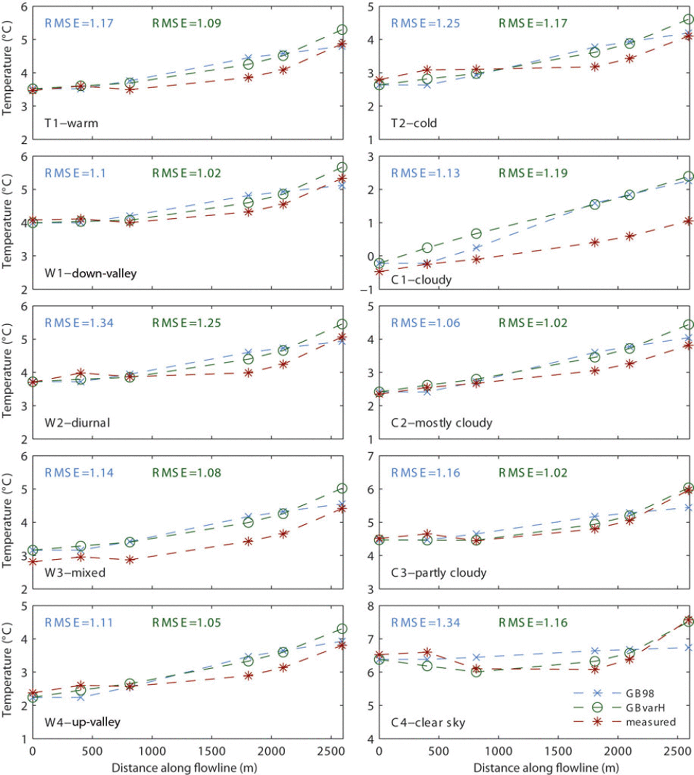
A number of results are apparent from Figure 5. In most cases, the application of a variable boundary layer thickness (GBvarH) is better able to represent the shape of the temperature profile along the flowline than the model assuming a constant boundary layer thickness. Under overcast conditions (C1), the model does not work well with a constant (GB98) or with a variable H (GBvarH). To support the visual evaluation of model performance (Fig. 5), we calculated the RMSE at each T-logger and the mean RMSE at all sites to quantitatively assess the model performance for different conditions. The application of a variable H reduces the RMSE for all conditions except cloudy days (cloud category C1) (Fig. 5), although improvements are minor for some categories. Both model versions are able to represent the almost linear shape of temperature that corresponds to very cold (cloudy) conditions, but neither can reproduce the correct slope. For all conditions except cloudy days the model performs best at TL7 and TL8 (followed by TL9 and TL2), indicating that it works best on the lower glacier section under conditions favourable to the development of katabatic wind. The improvement allowed by varying H is stronger on the lower section of the glacier under clear-sky conditions (with a mean improvement in RMSE of 12% in the upper part and of 17% in the lower), as well as under high temperatures and down-valley winds.

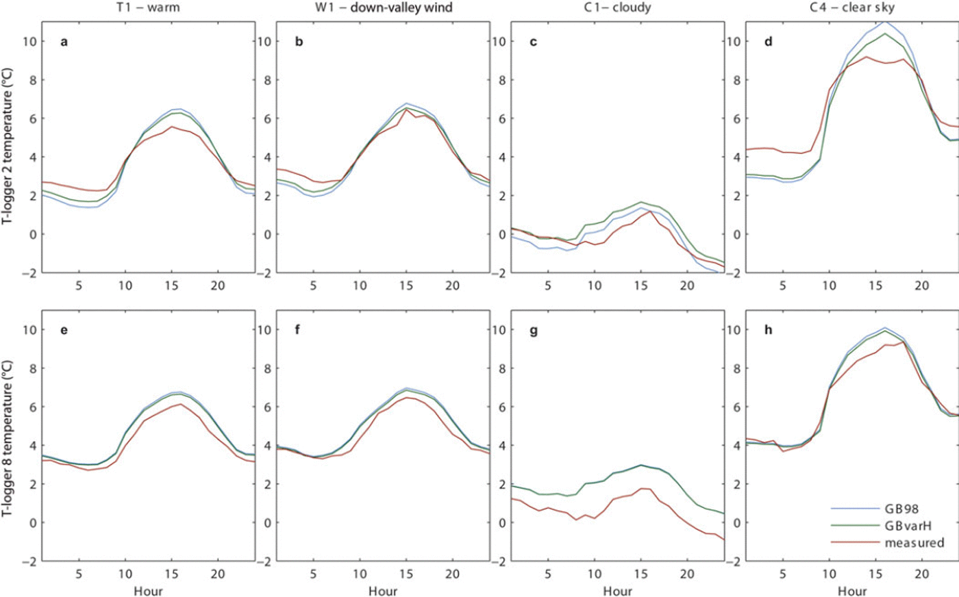
For down-valley wind conditions (W1) and high temperatures (T1) the fit for the mean values is good. This is also evident from analysis of the mean diurnal cycles at different locations (Fig. 6). It is clear that for all conditions except C1 (overcast days) the agreement between model simulations (with both options) and observations is better at the T-logger on the tongue (TL8, with RMSE of 1.03 and 1.05 for all conditions for GBvarH and GB98, respectively) than at the T-logger in the upper section of the glacier (TL2, with RMSE of 1.09 and 1.21 for all conditions for GBvarH and GB98, respectively). This is mainly due to the underestimation of temperature in the early morning and late evening by the model compared to the observation at TL2 (Fig. 6a, b and d), while this effect is no longer visible at TL8 (Fig. 6e, f and h). It is also evident that while no difference in performance can be observed between the two model versions at TL2, the model with variable H (GBvarH) works slightly better at the lower T-logger. Under cloudy, cold conditions, the fit between modelled and observed average temperatures is poorer for both models, especially at TL8 (Fig. 6c and g).

Fig. 6.

Mean diurnal cycle of measured air temperature compared with the results of the unmodified model (GB98) and model with variable H (GBvarH) for selected climatic conditions (described in Table 2) at TL2 in the upper section and TL8 in the lower section of the glacier.

6. Discussion and Conclusions

The along-glacier temperature distribution at HGdA is poorly represented by a constant linear LR. On the upper glacier, above ∼-2900ma.s.l., the LR is typically weak and often positive, indicating a shallow boundary layer and strong temperature stratification in the lowest few metres of the atmosphere. Below 2900 m a.s.l. on the glacier tongue, LRs are highly variable but frequently strongly negative, particularly when katabatic winds develop. Averaged over the entire glacier over the measurement period, the mean LR is less negative than the ELR. Use of a constant LR calibrated with local data improves the fit to observed temperature and results in a reduced RMSE. It should be kept in mind, however, that a large number of data were used to derive the CLRcal and these might not be commonly available. The two methods tested as alternative to a constant LR, GB98 and GBvarH, reduce the RMSE further. The GB98 model in its unmodified form over- or underestimates temperature at most locations and in most conditions, whereas GBvarH better captures the shape of the temperature profile along the flowlinefor most of the weather conditions considered, even though an overestimation is still evident. Hence, the assumption of a constant thickness of the glacier boundary layer does not seem to hold for HGdA. The variability in H was also stated by various authors and partly ascribed to the larger fetch for katabatic winds towards the glacier tongue (e.g. Reference Strasser, Corripio, Pellicciotti, Burlando, Brock and FunkStrasser and others, 2004; Reference Shea and MooreShea and Moore, 2010). The correspondence of mainly down-valley winds (W1) with high temperature agrees with the general prerequisite of a high temperature deficit favouring the development of katabatic wind (e.g. Reference OhataOhata, 1989; Reference Greuell, Knap and SmeetsGreuell and others, 1997; Reference Klok, Nolan and Van den BroekeKlok and others, 2005; Reference PellicciottiPellicciotti and others, 2008; Reference Shea and MooreShea and Moore, 2010). Under such conditions the GB98 model would be expected to work best, because the main requirements, the presence of a glacier wind and temperatures higher than 0°C, are fulfilled (see Reference Greuell and BöhmGreuell and Böhm, 1998). For clear-sky days (C4), as well as partly cloudy days (C3), the better performance of GBvarH on the lower part of the glacier corresponds to the better development of katabatic winds further down on the glacier due to topographic constraints (e.g. Reference Strasser, Corripio, Pellicciotti, Burlando, Brock and FunkStrasser and others, 2004; Reference Shea and MooreShea and Moore, 2010), such as the narrowing towards the tongue. High radiation on sunny and clear-sky days (C3 and C4) produces warm ambient air that is cooled by the ice surface (Reference Stenning, Banfield and YoungStenning and others, 1981), and the strong adiabatic warming on the lower part of the tongue is well captured by the GBvarH model. In contrast, the poor performance on cloudy days (C1), when temperatures are overestimated for most of the glacier, might be due to the fact that solar warming is reduced by the presence of clouds, and the lower temperature deficit prevents the development of katabatic flows, a prerequisite of the model (Reference Greuell and BöhmGreuell and Böhm, 1998). A possible reason for the poor performance of GB98, especially on the tongue, might be local effects. The influence of warming from surrounding slopes and debris patches could be an additional explanation for the steep increase in temperature at TL9, as mixing of warm air originating from debris-covered areas starting above TL9 with cold air moving downwards along the glacier could potentially influence the observed temperature. However, it is impossible to test such hypotheses without additional measurements. The other process that could be responsible for such warming is longwave radiation emission. At the glacier tongue the valley narrows to ∼500m width, so emission from the snow-free slopes might be more important than in the upper section. It is difficult to identify the main reasons for the observed temperature variability with the limited number of data available, and our study clearly points to the need to improve our understanding of temperature variability over glaciers. To quantify these local effects, the number of measurement sites should be expanded.

The conclusion that GBvarH works better than the original model means that we need a variable LR (length scale) in the model which can be due to an actual variability in H along the glacier flowline or to a variable cH. The validity of the assumption that cH is constant should be investigated by full energy-balance calculations, while more knowledge should be gained of the actual height of the GBL as well as its variability in space and main controls.

Some studies have found katabatic wind acceleration at night following radiative cooling (Reference Manins and SawfordManins and Sawford, 1979; Reference Horst and DoranHorst and Doran, 1986). The model is able to capture this possible behaviour in the lower part of the glacier, but underestimates temperature in the upper part (Fig. 6). This again suggests a strong temperature stratification in the lowest few metres of the atmosphere in the upper part of the glacier, where the boundary atmospheric layer is poorly developed due to a short fetch. Under such conditions, the 2 m measurement height is likely to be outside the ‘constant flux layer’ where the atmosphere is fully adjusted to the underlying surface, and a basic assumption of most energy-balance melt models will not be met in any case. As above, only more data on the height and characteristics of the GBL can provide a clear explanation for the observed variability at night.

The main conclusions of this study are that:

1. 1. The GB98 model provides a modest improvement over the assumption of a constant LR, even when locally calibrated, as demonstrated by a reduction of ∼ 7 % in the RMSE.

2. 2. For HGdA, the model works better when different glacier boundary layer thicknesses, H, are used for different sections of the glacier, as it captures the shape of the along-glacier temperature distribution and replicates the actual temperatures better.

3. 3. The model works better for clear-sky conditions and high temperatures, as the greater temperature deficit typical of these cases favours the development of a katabatic wind, which commonly occurs under sunny summer conditions.

4. 4. The model does not work well for cloudy conditions.

5. 5. It is also apparent from our results that no readily applicable model exists to derive distributed temperature fields over a glacier, nor can any be developed without additional measurements that will shed light on the height and characteristics of the KBL.

Overall, the performance of GB98 is found to be acceptable under conditions and in locations where a katabatic wind can develop, and represents an improvement over the use of a constant LR. However, different models for air temperature distribution are needed: in areas where the fetch is short or gradients are shallow; under cool and/or cloudy conditions; and when synoptic forcing of the wind dominates. Ourresults provide evidence for a possible variability of the height of the GBL that should be tested experimentally. Our measurements are inadequate to investigate the height and structure of the GBL, which would require tower measurements at different heights. Our results, however, seem to clearly call for further experiments and should give inputs for this sort of investigation. The finding that better results can be obtained by allowing the height of the GBL to vary along the glacier flowline should be tested for other sites.

We have compared four options for modelling air temperature with respect to their ability to reproduce the observed temperatures. Differences are evident but are generally small. The effect that each method would have on the magnitude of simulated melt and mass balance should also be evaluated.

GB98 and GBvarH can partly explain the low sensitivity of GBL temperature to external atmospheric temperature changes, and so help to address an important challenge in estimating glacier response to climatic changes. Successful application of the model requires knowledge of the initiation point for katabatic flows, however, and this will probably require local calibration data in most cases. Supported by new field data, future research should focus on incorporating different physical conditions and topographic effects in order to develop a model able to reproduce temperature time series throughout the glacier.