


1. Introduction
Vortex instabilities are recognized to be fundamental in understanding various phenomena in natural and engineering flows. For example, complex three-dimensional structures resulting from vortex instabilities often play an important role in the transition to turbulence. Coherent vortical motions and associated dynamics continue to persist in the turbulent regime as well (Pullin & Saffman Reference Pullin and Saffman1998). Several previous studies (Leibovich Reference Leibovich1978; Kerswell Reference Kerswell2002; van Heijst & Clercx Reference van Heijst and Clercx2009) have therefore addressed various aspects of vortex instabilities using laboratory experiments, numerical simulations and stability analyses. Furthermore, in stratified mixing layers, small-scale vortex instability mechanisms influence strongly the mixing efficiency in the turbulent regime that follows (Mashayek, Caulfield & Peltier Reference Mashayek, Caulfield and Peltier2013; Mashayek & Peltier Reference Mashayek and Peltier2013). In this paper, we perform a local stability analysis of the vortices that result from the Kelvin–Helmholtz (KH) instability, in both homogeneous and stably stratified shear flows.
The KH instability manifests in plane shear flows that contain an inflection point in the one-dimensional velocity profile. In the presence of stable stratification, often encountered in the atmosphere and the ocean, the KH instability occurs if the stratification is sufficiently weak. However, if  $ Ri >0.25$ is satisfied everywhere in an inviscid stratified parallel flow, then no linear instability is possible (Howard Reference Howard1961; Miles Reference Miles1961). Here, the Richardson number $ Ri $ is a measure of the ratio between the stratification and shear effects. The primary KH instability that occurs for $ Ri <0.25$ results in the formation of an array of vortices (Thorpe Reference Thorpe1973) that are connected by braid-like regions, with the resulting flow characterized by the presence of elliptic and hyperbolic points. Three-dimensional secondary instabilities of these two-dimensional vortical flows that result from a primary KH instability represent an important mechanism in the transition to turbulence in these flows.
Extensive global mode linear stability analyses, along with energy budget calculations, have been reported for the two-dimensional KH vortices that form in homogeneous and stratified shear flows (Klaassen & Peltier Reference Klaassen and Peltier1985c, Reference Klaassen and Peltier1991; Smyth & Peltier Reference Smyth and Peltier1991; Caulfield & Peltier Reference Caulfield and Peltier2000; Smyth Reference Smyth2003); all these studies presented the temporal evolution of the secondary instability characteristics by considering a quasi-steady base flow at different times. Klaassen & Peltier (Reference Klaassen and Peltier1985c) performed a global mode stability analysis on the numerically generated two-dimensional base flows that result from the primary KH instability for fixed parameter values of  $ {\textit {Re}} = 500$ (where $ {\textit {Re}}$ is the Reynolds number associated with the initial one-dimensional shear flow) and $ Ri = 0.07$. They report three-dimensional instabilities that are convective in nature, with the corresponding eigenmodes focused in the statically unstable regions of the base flow. Klaassen & Peltier (Reference Klaassen and Peltier1991) extended the study of Klaassen & Peltier (Reference Klaassen and Peltier1985c) to investigate the effects of Richardson number on the three-dimensional secondary instabilities, but at $ {\textit {Re}} = 300$. They conclude that the base flow shear drives the secondary instabilities at early times for all $ Ri $. In contrast, the secondary instabilities at large times derive their energy from convective overturning in the vortex centres for Richardson numbers in the range $0.065\le Ri \le 0.13$. In summary, global mode analyses have revealed an elliptic secondary instability at the centre and a dominant hyperbolic instability at the vortex edge in homogeneous shear flows. In stratified flows, the central core elliptic instability, along with a more dominant convective instability near the periphery of the vortex, has been reported.
More recent global instability studies (Mashayek & Peltier Reference Mashayek and Peltier2012a,Reference Mashayek and Peltierb) at relatively larger  $ {\textit {Re}}$ ( $ {\textit {Re}}\ge 1000$) have identified a ‘zoo’ of secondary instabilities and investigated their relative importance as a function of time, $ {\textit {Re}}$ and $ Ri $. Apart from the elliptic and hyperbolic instabilities present for the homogeneous case, stratification has been shown to introduce a combination of small-wavenumber (secondary shear instability, secondary core deformation instability) and large-wavenumber (secondary convective instability, stagnation point instability, localized core vortex instability) secondary instabilities. The large-wavenumber secondary instabilities represent the focus of this paper. Specifically, we perform a local stability analysis to complement the results from previous global mode approaches, particularly in terms of identifying specific regions of various secondary instabilities, their evolution and associated mechanisms. As such, it is not known which of the instabilities identified in the global stability analysis can actually be recovered using the local stability approach. Our study addresses this question, and in the process, explores the relation between the local and global stability approaches for the homogeneous and stratified KH vortices. In a broader sense, the current study helps to evaluate the usefulness of the computationally efficient local stability approach in characterizing various secondary instabilities in stratified mixing layers under various conditions.
The local stability approach (Lifschitz & Hameiri Reference Lifschitz and Hameiri1991) employs the Wentzel–Kramers–Brillouin–Jeffreys (WKBJ) approximation to investigate three-dimensional short- wavelength instabilities in a given base flow. The local stability equations, which govern the evolution of leading-order perturbation amplitudes on fluid trajectories in the base flow, have been used previously to investigate various instability mechanisms in several idealized vortex models. The local approach has provided significant insight into the effect of various factors like strain, background rotation, stratification and axial flow on vortex models such as Stuart vortices, Taylor–Green vortices and a Rankine vortex (Miyazaki & Fukumoto Reference Miyazaki and Fukumoto1992; Miyazaki Reference Miyazaki1993; Dizès & Eloy Reference Dizès and Eloy1999; Godeferd, Cambon & Leblanc Reference Godeferd, Cambon and Leblanc2001; Mathur et al. Reference Mathur, Ortiz, Dubos and Chomaz2014; Nagarathinam, Sameen & Mathur Reference Nagarathinam, Sameen and Mathur2015). Being computationally inexpensive, the local approach has helped to identify centrifugal, elliptic and hyperbolic instabilities on specific streamlines in the strongly non-parallel model vortex flows. The local approach has also been used on numerically simulated two-dimensional wake flows (Gallaire, Marquillie & Ehrenstein Reference Gallaire, Marquillie and Ehrenstein2007; Citro et al. Reference Citro, Giannetti, Brandt and Luchini2015; Giannetti Reference Giannetti2015; Jethani et al. Reference Jethani, Kumar, Sameen and Mathur2018), but not on a numerically simulated base flow in which stratification plays an important role.
Previous studies using the local stability approach have identified centrifugal, elliptic and hyperbolic instabilities in various idealized vortex models (Godeferd et al. Reference Godeferd, Cambon and Leblanc2001). The centrifugal instability on a given streamline is often associated with the most unstable wave vector being purely spanwise. In contrast, the most unstable wave vector associated with the elliptic instability makes an angle of around  ${\rm \pi} /3$ with the spanwise direction (Kerswell Reference Kerswell2002). The hyperbolic instability (Leblanc Reference Leblanc1991), which occurs on streamlines that pass through regions in the neighbourhood of hyperbolic points, is also characterized by purely spanwise perturbations being most unstable. It is, however, important to note that these classical signatures of various instabilities can be modified significantly in the presence of factors such as stratification (Miyazaki & Fukumoto Reference Miyazaki and Fukumoto1992; Miyazaki Reference Miyazaki1993), background rotation (Godeferd et al. Reference Godeferd, Cambon and Leblanc2001) and axial flow (Mathur et al. Reference Mathur, Ortiz, Dubos and Chomaz2014; Nagarathinam et al. Reference Nagarathinam, Sameen and Mathur2015), and are hence used as guidelines rather than strict criteria in our study.
Mixing layer vortices in homogeneous flows have often been represented using the idealized model of Stuart vortices (Pierrehumbert & Widnall Reference Pierrehumbert and Widnall1982; Potylitsin & Peltier Reference Potylitsin and Peltier1999). Klaassen & Peltier (Reference Klaassen and Peltier1991) and Rogers & Moser (Reference Rogers and Moser1992), however, report that Stuart vortices may not capture all the secondary instability characteristics in homogeneous mixing layers. Furthermore, the relevance of the Stuart vortices model to describe mixing layer vortices in a stratified environment is also unclear. In this paper, we perform local stability calculations on KH vortices simulated using two-dimensional numerical simulations, thus eliminating the approximations associated with idealized vortex models. Three-dimensional numerical simulations (Metcalfe et al. Reference Metcalfe, Orszag, Brachet, Menon and Riley1987; Staquet & Riley Reference Staquet and Riley1989; Rogers & Moser Reference Rogers and Moser1992; Fritts et al. Reference Fritts, Palmer, Andreassen and Lie1996; Palmer, Fritts & Andreassen Reference Palmer, Fritts and Andreassen1996; Caulfield & Peltier Reference Caulfield and Peltier2000; Mashayek & Peltier Reference Mashayek and Peltier2011) and laboratory experiments (Thorpe Reference Thorpe1987) have revealed the emergence of small-scale coherent structures in homogeneous and stratified mixing layer vortices. Global stability analysis (Smyth & Peltier Reference Smyth and Peltier1991; Caulfield & Peltier Reference Caulfield and Peltier2000; Mashayek & Peltier Reference Mashayek and Peltier2012a,Reference Mashayek and Peltierb) has also reported on large-wavenumber instabilities in both homogeneous and stratified cases, thus suggesting that the secondary instabilities may be amenable to the short-wavelength approximation that the local approach assumes. In addition to the demonstration of local stability analysis and its relation to what is known from global stability analysis, our specific objectives include: (i) an identification of those instabilities that can be recovered using the local stability approach; (ii) an identification of localized regions where the short-wavelength instabilities emerge and evolve; (iii) an evaluation of the influence of shear and buoyancy on the instability characteristics; (iv) an investigation of the variation of the instability characteristics as a function of the Richardson number; and (v) an estimation of the orientation of the flow structures that may develop as a result of the dominant instabilities.
In § 2, we present the details of two-dimensional numerical simulations used to generate the base flows, the local stability equations and the methods adopted to compute growth rates associated with various instabilities. Section 3 presents the results for the homogeneous (unstratified) base flow, followed by a detailed investigation of a representative stratified scenario. A systematic study on the effects of  $ Ri $ is presented in § 4, followed by our discussion and conclusions in § 5.
2. Theory and methods
We study three-dimensional short-wavelength instabilities on the two-dimensional vortical flow that develops upon solving numerically non-dimensional forms of the mass, momentum and buoyancy equations in the limit of the Boussinesq approximation (Mkhinini, Dubos & Drobinski Reference Mkhinini, Dubos and Drobinski2013):
 $$\begin{gather} \boldsymbol{\nabla}\boldsymbol{\cdot}\boldsymbol{u} = 0, \end{gather}$$
 $$\begin{gather}\frac{\partial{\boldsymbol{u}}}{\partial{t}} + (\boldsymbol{u}\boldsymbol{\cdot}\boldsymbol{\nabla})\boldsymbol{u} + \boldsymbol{\nabla} p = \frac{1}{{\textit{Re}}}\,\nabla^{2} \boldsymbol{u} + Ri \,B\,\boldsymbol{e}_y, \end{gather}$$
 $$\begin{gather}\frac{\partial B}{\partial t} + (\boldsymbol{u}\boldsymbol{\cdot}\boldsymbol{\nabla})B = \frac{1}{{\textit{Re}}\,Pr}\,\nabla^{2} B, \end{gather}$$
on a two-dimensional Cartesian grid  $(x,y)=(x_d/h,y_d/h)\in [-L_d/2h,L_d/2h]\times (-\infty,\infty )$ (see figure 1(a) for a schematic), with initial conditions (denoted by superscript $i$)
$i$)
 \begin{equation} \boldsymbol{u}^{i} = \frac{\boldsymbol{u}_d^{i}}{U} = \tanh(y)\,\boldsymbol{e}_x,\quad B^{i} = \frac{B_d^{i}}{N^{2}h} = \tanh(y). \end{equation}
The various quantities – spatial coordinates, time, velocity, pressure and buoyancy – with and without the subscript  $d$ are dimensional and non-dimensional, respectively. The dimensional buoyancy is defined as $B_d = g(1-\rho _d/\rho _{ref})$, where $\rho _d$ and $\rho _{ref}$ are the dimensional density field and constant reference density, and $g$ is the magnitude of the acceleration due to gravity that acts along negative $\boldsymbol {e}_y$. Spatial coordinates and time have been non-dimensionalized by the shear layer half-width $h$ and the advective time scale $h/U$, respectively, and $\boldsymbol {e}_x$ and $\boldsymbol {e}_y$ are the unit vectors along $x$ and $y$. Buoyancy and pressure are non-dimensionalized by $N^{2}h$ and $\rho _{ref}U^{2}$, respectively, where $N$ is the Brunt–Väisälä frequency at $y = 0$ in the initial condition (2.4a,b). The non-dimensional parameters that govern the flow dynamics are the Reynolds number $ {\textit {Re}}$ ( $= Uh/\nu$), the Richardson number $ Ri $ ( $= N^{2}/(U/h)^{2}$), and the Prandtl number $Pr$ ( $= \nu /\kappa$), where $\nu$ and $\kappa$ are the kinematic viscosity and the buoyancy diffusivity, respectively.
(a) A schematic of the computational flow domain and initial conditions (buoyancy  $B_d^{i}$ and velocity $u_d^{i}$ on the left and right, respectively, with $B_0 = N^{2}h$) used for two-dimensional numerical simulation of KH vortices, where $L_d$ is the length of the computational domain, and $2h$ represents the width of both the shear layer and the buoyancy layer. (b) A few numerically extracted streamlines in the KH vortex on the $x$–
$x$– $y$ plane. Here, $P_1$ ( $\equiv (x_0,0$)) and $P_2$ ( $\equiv (-L_d/2h,y_0$)) are two representative initial conditions used to extract closed streamlines and open streamlines, respectively. An initial perturbation wave vector $\boldsymbol {k}^{i}$, making an angle $\theta ^{i}$ with the $z$-axis, of a three-dimensional perturbation that evolves on one of the extracted streamlines is also shown.

Throughout the current study, we assume  $( {\textit {Re}},Pr) = (300,1)$, and consider several values of $ Ri $ in the range $[10^{-8},0.225]$. The chosen values of $ {\textit {Re}}$ and $Pr$ allow us to make comparisons with the global analysis of Klaassen & Peltier (Reference Klaassen and Peltier1991). For numerical resolution, the vertical domain $y\in (-\infty,\infty )$ is mapped onto a finite domain using a $\tanh$ transformation, and the flow field is assumed to be unperturbed at $y\to -\infty$ and $y\to +\infty$ (Mkhinini et al. Reference Mkhinini, Dubos and Drobinski2013). Setting the dimensional horizontal extent of the computational domain ( $L_d = 4{\rm \pi} h$ in § 3, and $L_d = 14.7h$ in § 4) to be approximately the wavelength of the most unstable primary wave, along with periodic boundary conditions in the horizontal, allows us to simulate the evolution of one coherent vortex that forms as a result of the primary KH instability. We consider these simulated flow fields to be frozen at each instant and use them as steady base flows to extract corresponding closed and open streamlines, and subsequently solve the local stability equations on them. We note that our base flow contains only one KH vortex, and its stability characteristics will likely not capture the pairing instability (Klaassen & Peltier Reference Klaassen and Peltier1989).
For the local stability analysis (Lifschitz & Hameiri Reference Lifschitz and Hameiri1991), we consider a decomposition of the velocity, pressure and buoyancy fields into a sum of base flow (denoted by subscript  $B$) and perturbation (denoted by a prime) fields as $\boldsymbol {u} = \boldsymbol {u}_{B} + \boldsymbol {u}^{\prime }$, $p = p_B + p^{\prime }$, $B = b_B + b^{\prime }$, and substitute in the governing equations (2.1)–(2.3) to derive the linearized governing equations for the small perturbations. The perturbation fields, within the limits of the WKBJ approximation, are written as
 \begin{align} \{\boldsymbol{u}^{\prime},p^{\prime},b^{\prime}\} &= \exp{\left(\frac{{\rm i}\,\phi(\boldsymbol{x},t)}{\epsilon}\right)} [\{\boldsymbol{a}(\boldsymbol{x},t),\tilde{p}(\boldsymbol{x},t),b(\boldsymbol{x},t)\} \nonumber\\ &\quad +\epsilon\{\boldsymbol{a}_\epsilon(\boldsymbol{x},t),\tilde{p} _\epsilon(\boldsymbol{x},t), b_\epsilon(\boldsymbol{x},t)\} + \cdots], \end{align}
where  $\epsilon \ll 1$ is a small parameter, indicative of the perturbations being of short wavelength. The perturbation wave vector is given by $\boldsymbol {k} = \boldsymbol {\nabla }\phi /\epsilon$, where $\phi$ is a real-valued scalar function. Substituting the solution forms in (2.5) into the inviscid (no diffusion in both momentum and buoyancy) equations governing small-amplitude perturbations, and retaining only the $O(\epsilon ^{-1})$ and $O(\epsilon ^{0})$ terms, gives the local stability equations that govern the evolution of the wave vector and the leading-order perturbation amplitudes (Miyazaki & Fukumoto Reference Miyazaki and Fukumoto1992):
 $$\begin{gather} \frac{\mathrm{d}\boldsymbol{k}}{\mathrm{d}t} ={-}(\boldsymbol{\nabla} \boldsymbol{u}_B)^{{\rm T}}\boldsymbol{\cdot}\boldsymbol{k}, \end{gather}$$
 $$\begin{gather}\frac{\mathrm{d}\boldsymbol{a}}{\mathrm{d}t} ={-}(\boldsymbol{\nabla} \boldsymbol{u}_B)\boldsymbol{\cdot}\boldsymbol{a} + Ri \,b\,\boldsymbol{e}_y + \frac{\boldsymbol{k}}{|\boldsymbol{k}|^{2}}\,(2((\boldsymbol{\nabla} \boldsymbol{u}_B)\boldsymbol{\cdot}\boldsymbol{a})\boldsymbol{\cdot}\boldsymbol{k} - Ri \, b\,\boldsymbol{e}_y\boldsymbol{\cdot}\boldsymbol{k}), \end{gather}$$
 $$\begin{gather}\frac{\mathrm{d}b}{\mathrm{d}t} ={-} \boldsymbol{a}\boldsymbol{\cdot}\boldsymbol{\nabla} b_B, \end{gather}$$
along with the constraint of  $\boldsymbol {a}\boldsymbol {\cdot }\boldsymbol {k} = 0$ that is obtained from the continuity equation. Here, $\mathrm {d}/\mathrm {d}t = \partial /\partial t + \boldsymbol {u}_B\boldsymbol {\cdot }\boldsymbol {\nabla }$ is the material derivative in the base flow, i.e. equations (2.6)–(2.8) represent the evolution of $\boldsymbol {k}$, $\boldsymbol {a}$ and $b$ along fluid particle trajectories in the base flow $\boldsymbol {u}_B$.
We consider instantaneous snapshots of the numerically simulated two-dimensional flow fields to represent steady base flows in (2.6)–(2.8). The stability calculations are performed on all the closed streamlines, and the open streamlines that are close to the outer vortex boundary in the numerically simulated base flow (see figure 1b). For every streamline, we consider only those wave vectors that are periodic upon integrating (2.6) once along the entire streamline. Such periodic wave vectors are given by (Mathur et al. Reference Mathur, Ortiz, Dubos and Chomaz2014)
 \begin{equation} \boldsymbol{k} = \beta\,\boldsymbol{\nabla} \psi + \cos{\theta^{i}}\,\boldsymbol{e}_z, \end{equation}
where  $\psi (x,y)$ is the streamfunction describing the base flow through the relation $\boldsymbol {u}_B = (-\partial \psi /\partial y)\, \boldsymbol {e}_x + (\partial \psi /\partial x)\,\boldsymbol {e}_y$. Owing to the scale invariance of (2.6)–(2.8) with respect to $\boldsymbol {k}$, we restrict our calculations to $|\boldsymbol {k}^{i}| = 1$, and hence choose $\beta = \sqrt {(1-\cos ^{2}{\theta ^{i}})/|\boldsymbol {\nabla }\psi ^{i}|^{2}}$, with $\theta ^{i}$ representing the angle made by the initial wave vector $\boldsymbol {k}^{i}$ with the $z$-axis (depicted in figure 1b). For a given streamline, which is uniquely identified by the initial condition $(x_0>0,0)$ for a closed streamline, and $(-L_d/2h,y_0>0)$ or $(L_d/2h,-y_0)$ for an open streamline (figure 1b), we solve the perturbation amplitude evolution equations (2.7) and (2.8) for $1000$ different values of $\theta ^{i}$ in the range $[0,{\rm \pi} /2]$. The symmetry in the simulated flow field results in identical instability characteristics for the open streamlines above and below the centreline $y=0$. Hence the results for the open streamlines are presented only for the initial conditions given by $(-L_d/2h,y_0>0)$.
For each streamline, at a given  $\theta ^{i}$, (2.7) and (2.8) were integrated numerically using a fourth-order Runge–Kutta scheme from $0$ to $T$ for four different initial conditions, $\boldsymbol {a}^{i}_1 = [1, 0, 0, 0]^{\rm T}$, $\boldsymbol {a}^{i}_2 = [0, 1, 0, 0]^{\rm T}$, $\boldsymbol {a}^{i}_3 = [0, 0, 1, 0]^{\rm T}$ and $\boldsymbol {a}^{i}_4 = [0, 0, 0, 1]^{\rm T}$, where $\boldsymbol {a}^{i}_j = [a^{i}_x, a^{i}_y, a^{i}_z, b^{i}]^{\rm T}$, to obtain the final amplitude vectors $\boldsymbol {a}^{f}_1$, $\boldsymbol {a}^{f}_2$, $\boldsymbol {a}^{f}_3$ and $\boldsymbol {a}^{f}_4$. Here, $T$ is the time period over which a fluid particle traverses the entire streamline once. The growth rate, using results from Floquet theory (Chicone Reference Chicone2000), is then computed as
 \begin{equation} \sigma(x_0\text{ or }y_0,\theta^{i}) = (1/T)\max[{\textit{Re}}(\log(\lambda_j))], \end{equation}
where  $\lambda _j$ ( $1\le j\le 4$) are the eigenvalues of the $4\times 4$ matrix $\boldsymbol{\mathsf{M}} = [\boldsymbol{a}^f_1, \boldsymbol{a}^f_2, \boldsymbol{a}^f_3, \boldsymbol{a}^f_4]$. For the integration of (2.7) and (2.8), we discretize the time period $T$ by $4000$ equispaced time intervals. The function $\sigma (x_0\text { or } y_0,\theta ^{i})$ is calculated numerically at various time instances of the simulated base flows, which are assumed steady for the local stability calculations. It is noteworthy that three-dimensional instabilities are not allowed to appear in our two-dimensional numerical simulations that generate the base flows. This allows us to perform local stability calculations for arbitrarily large times, though a three-dimensional instability could occur at relatively earlier times in a three-dimensional numerical simulation.
The assumption of a steady base flow for growth rate computations may be valid only if the time scale associated with the growth rate is smaller than the time scale associated with the evolution of the numerically simulated base flow. Such a condition is satisfied reasonably if  $\sigma >\sigma _{KH}$, where $\sigma$ is the calculated growth rate for the perturbations that grow on the simulated base flow, and $\sigma _{KH}$ is the growth rate associated with the evolution of the simulated primary vortex. Here, we compute $\sigma _{KH}$ based on the evolution of the kinetic energy associated with the flow deviation from the initial conditions, as given in equation (3.7) of Klaassen & Peltier (Reference Klaassen and Peltier1991). The extent of validity of the condition $\sigma >\sigma _{KH}$ is presented wherever appropriate in § 3.
The results are organized such that § 3 compares and contrasts the stability characteristics of the homogeneous case (approximated by  $ Ri = 10^{-8}$) and one representative stratified case ( $ Ri = 0.08$). Section 4 is then focused on a systematic investigation of the variation of the instability characteristics with $ Ri $. A summarized discussion of our results and conclusions is then provided in § 5.
3. Results: homogeneous versus stratified
Base flows were generated for the homogeneous case (by assigning  $ Ri = 10^{-8}$ in the two-dimensional simulations) and one representative stratified case ( $ Ri = 0.08$) at $ {\textit {Re}}=300$ for every integer time $t$ until
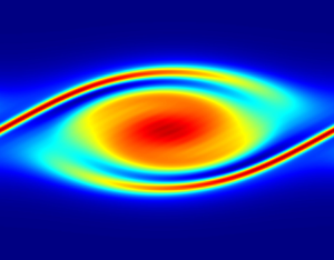
  $t = 200$. Figure 2 shows the vorticity field ( $\omega_z$) obtained using numerical simulations at three different times for the homogeneous case (figures 2a–c) and six different times for the stratified case (figures 2d–i). The black dashed line in each panel of figure 2 represents the outermost numerically extracted closed streamline (denoted by $x_0 = x_{0_l}$) in the flow at the corresponding time. For the purposes of this paper, we refer to the region enclosed by the outermost closed streamline as the KH vortex, and the braid region (top left and bottom right of the KH vortex, which are the regions where the flow moves away from the hyperbolic point) lies in the neighbourhood of this outermost streamline. Since the braid region lies partly inside the KH vortex, associated instabilities could occur on both the closed and open streamlines in the neighbourhood of the outermost closed streamline. During the evolution of the homogeneous flow, the vortex core remains the site of strongest clockwise vorticity as the vorticity in the braids gets dissipated quickly (figures 2a–c). Although the early-time evolution of the stratified flow (figure 2d) is similar to the homogeneous case, the braids become regions of strong clockwise vorticity at intermediate times (figures 2f ,g) as the KH vortex reaches its climax state (Klaassen & Peltier Reference Klaassen and Peltier1985b, Reference Klaassen and Peltier1991). As the stratified flow evolves further, the vorticity in the braids gets drained as bands of near-zero vorticity from the vortex core approach the braid regions (figure 2h). Although this draining of vorticity from the braid region is known to mark the onset of the two-dimensional pairing instability (Mashayek & Peltier Reference Mashayek and Peltier2012a), we do not observe this in our simulations since our choice of the computational domain permits the evolution of only a single KH vortex. Finally, at $t = 170$ (figure 2i), a braid structure with a near-zero vorticity band just inside the last closed streamline is seen again, albeit with weaker vorticity gradients than at $t=86$. A detailed discussion of the evolution of the two-dimensional KH vortex, and associated energetics, can be found in previous studies: Klaassen & Peltier (Reference Klaassen and Peltier1985b) studied the range $300\le {\textit {Re}}\le 900$ at $ Ri = 0.07$, and Caulfield & Peltier (Reference Caulfield and Peltier2000) studied the range $0\le Ri \le 0.1$ at $ {\textit {Re}} = 750$.
Vorticity field ( $\omega_z$) obtained using two-dimensional numerical simulations along with the outermost numerically extracted closed streamline (black dashed line) at various times: (a) $t = 40$, (b) $t = 60$, and (c) $t = 100$, for the homogeneous case $( {\textit {Re}}, Ri ) = (300,10^{-8})$; and (d) $t = 55$, (e) $t = 60$, ( f) $t = 70$, (g) $t = 86$, (h) $t = 108$ and (i) $t = 170$, for the stratified case $( {\textit {Re}}, Ri ) = (300,0.08)$. Animations of the vorticity fields for the homogeneous and stratified cases can be found in supplementary movies 1 and 2, respectively, available at https://doi.org/10.1017/jfm.2022.394.

For every integer value of  $t$, 100 different closed streamlines (denoted by $x_0$, with $x_0>0$) and 500 open streamlines (denoted by $y_0$, with $y_0>0$) were extracted, with $x_0 = 0$ and $y_0 = 0$ representing the elliptic (vortex centre) and the hyperbolic stagnation points, respectively. Growth rate calculations were done on each of these streamlines for 1000 different values of $\theta ^{i}$ in the interval $[0,{\rm \pi} /2]$, allowing us to plot the growth rate $\sigma$ as a function of the streamline location ( $x_0$ for a closed streamline, $y_0$ for an open streamline) and the initial wave vector angle ( $\theta ^{i}$), at every instant of time (§ 3.1). The temporal evolution of the dominant instability characteristics are then plotted in § 3.2, followed by a summary in § 3.3. In § 3.4, we discuss the relation between convective instabilities and the statically unstable layers that form in the stratified case.
3.1. Instability characteristics
3.1.1. Closed streamlines
Figures 3(a–c) show the variation of the computed growth rate  $\sigma$ (2.10) on the closed streamlines for the homogeneous case as a function of $x_0$ on the $x$-axis and the initial wave vector angle $\theta ^{i}$ on the $y$-axis at three different times: $t = 40$, 60 and 100. At $t = 40$ (figure 3a), the vortex centre ( $x_0 = 0$) is evidently unstable, with the corresponding growth rate attaining a maximum 0.147 at $\theta ^{i} = 51.4^{\circ }$, a value close to ${\rm \pi} /3$. It is well known that elliptic instability is characterized by the corresponding most unstable wave vector occurring at $\theta ^{i} = {\rm \pi}/3$ (Bayly Reference Bayly1986; Kerswell Reference Kerswell2002), owing to which we conclude that the vortex core at $t = 40$ is susceptible to inviscid elliptic instability. The streamlines in the immediate neighbourhood of the vortex centre, which are not necessarily exactly elliptic, are observed to be unstable in the range $26.7^{\circ }\le \theta ^{i}\le 74.1^{\circ }$. The range of unstable $\theta ^{i}$ increases as we go away from the vortex centre, with the corresponding most unstable $\theta ^{i}$ moving towards $\theta ^{i}= 0$ as we approach the edge of the vortex. The instability at the edge of the vortex is hyperbolic, as signified by the presence of a hyperbolic point in its immediate neighbourhood and the most unstable $\theta ^{i}$ occurring close to $\theta ^{i} = 0$. We recall from earlier studies (Leblanc Reference Leblanc1991; Godeferd et al. Reference Godeferd, Cambon and Leblanc2001) that hyperbolic instability, in general, is most severe for purely spanwise perturbations, i.e. $\theta = 0$. In summary, at $t=40$, the vortex core and the edge are susceptible to elliptic and hyperbolic instabilities, respectively, and the intermediate streamlines exhibit a combination of both. As indicated by the location of maximum $\sigma$ over the entire $x_0$– $\theta ^{i}$ plane (red circle in figure 3a), the elliptic instability at the core dominates the hyperbolic instability at the edge at $t = 40$.
Growth rate  $\sigma$ (on closed streamlines) as a function of the streamline location $x_0$ and the initial perturbation wave vector angle $\theta ^{i}$ for (a–c) $( {\textit {Re}}, Ri ) = (300,10^{-8})$, and (d–i) $( {\textit {Re}}, Ri ) = (300,0.08)$, at the same times as in figure 2. The points $(x_0,\theta ^{i})$ corresponding to maximum $\sigma$ are marked with red circles. Animations of the instability characteristics for the homogeneous and stratified cases can be found in supplementary movies 1 and 2, respectively.

At a later time,  $t = 60$ (figure 3b), the variation of $\sigma$ is qualitatively similar to that at $t = 40$, but with a thinner and weaker instability band (i.e. spanning a smaller range in $\theta ^{i}$) at the core ( $x_0 = 0$), and the hyperbolic instability seemingly extending further towards the vortex centre from the vortex edge. The location of maximum $\sigma$, as denoted by the red circle, has now moved to the vortex edge, suggesting that almost purely spanwise perturbations ( $\theta ^{i}\approx 0$) at the vortex edge are likely to grow fastest at $t = 60$. At the much later time $t = 100$ (figure 3c), the qualitative structure of $\sigma$ is very similar to that at $t = 60$, and the hyperbolic instability at the vortex edge remains dominant. Finally, the results in figures 3(a–c) suggest that centrifugal instability is not present at any time for the homogeneous case; we discuss this aspect again in § 3.2.1.
For the stratified case (figures 3d–i), the elliptic instability at the vortex core is dominant at  $t = 55$ (figure 3d), with its corresponding maximum $\sigma$ ( $= 0.155$) occurring at $\theta ^{i} = 49.5^{\circ }$. The growth rate magnitude of this elliptic instability is comparable to its counterpart in the homogeneous case (figure 3a), suggesting that the stratification does not influence significantly the elliptic instability characteristics at early times. The hyperbolic instability, however, seems strongly affected by stratification, as seen by the multiple bands of instability near the vortex edge in figure 3(d). We recall from figure 3(a) that no such complex features were present for the homogeneous case. The complex instability features at the vortex edge in figure 3(d) could be attributed to either (i) the existing hyperbolic instability (in the homogeneous case) modified by the stratification, or (ii) the emergence of new instabilities associated with the vortex edge/braid region of the stratified case. In relation to point (i), earlier studies by Godeferd et al. (Reference Godeferd, Cambon and Leblanc2001) have reported a similar effect that background rotation has on the hyperbolic instability in Stuart vortices. In our study, the in-plane buoyancy variations could be playing the role of spatially varying Coriolis forces that result from the background rotation. In relation to point (ii), figure 1 of Mashayek & Peltier (Reference Mashayek and Peltier2012b) provides a summary of the various instabilities at the vortex edge/braid region in the presence of stratification, albeit at a $ {\textit {Re}}$ larger than 300.
Another distinguishing feature at  $t = 55$ (figure 3d) that is not present in the homogeneous case is the occurrence of instability at $\theta ^{i} = 0$ for the streamlines in and around the vortex core. This instability branch, which seems distinct from the elliptic instability, moves away from the vortex centre with time and is characterized by its corresponding most unstable $\theta ^{i}$ hovering around zero. We henceforth refer to this new instability as the convective branch, owing to its relation with statically unstable layers, as discussed later in § 3.4. At $t = 60$ (figure 3e), while the elliptic instability at the core and the instabilities at the edge are still present, an intermediate streamline that is far from both the vortex core and the edge is the most unstable. The most unstable streamline at $x_0 = 2.06$ is affected simultaneously by the elliptic instability of the core and the convective band that has moved away from the core, owing to which the corresponding most unstable $\theta ^{i}$ ( $=44.0^{\circ }$) has moved away from ${\rm \pi} /3$. At a later time, $t = 70$ (figure 3f), the convective branch is the most dominant, with the corresponding $(x_0,\theta ^{i}) = (x_0^{*},\theta ^{i^{*}}) = (3.09,0)$. This convective band moves further to the right with time, and is strongest at $x_0^{*} = 4.30$, with the corresponding $\theta ^{i^{*}}$ again being zero at $t = 86$ (figure 3g). Furthermore, at $t = 86$, we observe a second band of convective instability centred around $x_0 = 2.06$. At a later time, $t = 108$ (figure 3h), this second convective band has become the most dominant, while the first convective band seems to have moved to the braid region. At $t = 108$, we also observe a third convective band centred around $x_0 = 1.82$. The elliptic instability at the centre influences the second convective band strongly enough to move the most unstable $\theta ^{i}$ to around $\theta ^{i^{*}} = 28.3^{\circ }$. At large times ( $t = 170$ shown in figure 3i), multiple convective bands, which emerged at the vortex core at earlier times and then moved away, have coalesced into a single convective instability region with $x_0^{*} = 4.79$. Also, at these large times, the convective instability bands emerging from the centre, and the braid instabilities are significantly weaker compared to earlier times owing to buoyancy and momentum diffusion in the base flow. In summary, the instability characteristics at large times contain an elliptic branch at the vortex centre, the dominant convective branch close to but inside the periphery of the vortex, and hyperbolic and braid instabilities associated with the vortex edge.
Finally, we also observe other weaker instabilities at intermediate times. For example, at  $t = 86$ (figure 3g), we find relatively weak instability regions for $\theta ^{i} \gtrsim {\rm \pi}/3$ in and around the convective instability regions. Interestingly, they extend all the way to $\theta ^{i} = {\rm \pi}/2$, which corresponds to two-dimensional perturbations. These weaker instabilities, present only in the stratified case and not the homogeneous case, potentially could be related to one or more of the instabilities associated with the core and edge regions of the KH vortex (Staquet Reference Staquet1995; Mashayek & Peltier Reference Mashayek and Peltier2012a,Reference Mashayek and Peltierb).
3.1.2. Open streamlines
In figure 4, we show the instability characteristics, i.e.  $\sigma$ as a function of $y_0$ and $\theta ^{i}$, for the open streamlines in the homogeneous (figures 4a–c) and stratified (figures 4d–i) cases. Small values of $y_0$ in these plots correspond to open streamlines that are in the immediate neighbourhood of the outermost closed streamline in the KH vortex. For the homogeneous case, at all three times (figures 4a–c), the $\sigma$ versus $\theta ^{i}$ variations for $y_0\approx 0$ resemble those at the outermost closed streamline. Specifically, for the first open streamline, $\sigma$ is maximum at $\theta ^{i} = 0$, then decreases monotonically towards zero as $\theta ^{i}$ approaches ${\rm \pi} /2$. For the outermost closed streamline, $\sigma$ is maximum at a finite $\theta ^{i}$ close to zero, then decreases as $\theta ^{i}$ increases, and finally becomes zero at and beyond a threshold value of $\theta ^{i}$ (figures 3a–c). The hyperbolic instability at the vortex edge is thus captured by the first open streamline as well. As $y_0$ is increased from 0, the most unstable $\theta ^{i}$ moves away from zero (figures 4a–c), much like the hyperbolic instability behaviour on the streamlines just inside the outermost closed streamline.
Growth rate  $\sigma$ (on open streamlines) as a function of the streamline location $y_0$ and the initial perturbation wave vector angle $\theta ^{i}$ for (a–c) $( {\textit {Re}}, Ri ) = (300,10^{-8})$, and (d–i) $( {\textit {Re}}, Ri ) = (300,0.08)$, at the same times as in figure 2. The points $(y_0,\theta ^{i})$ corresponding to maximum $\sigma$ are marked with red circles. Animations of the instability characteristics for the homogeneous and stratified cases can be found in supplementary movies 1 and 2, respectively.

In the stratified case  $ Ri = 0.08$, at early times (figures 4d–f), the small $y_0$ region that is right outside the KH vortex shows additional bands of instability present alongside the instability already seen in the homogeneous case (figures 4a–c). Comparing the instability characteristics at large $x_0$ in the closed streamlines analysis and at small $y_0$ in the open streamlines analysis, we conclude that the bands of instability seen in figures 3(d–f) and 4(d–f) are likely to be associated with the braid region. In other words, a weaker hyperbolic instability (when compared to the homogeneous case), and new instabilities associated with the braid region that forms due to stratification, are both observed in the open streamlines right outside the KH vortex for $ Ri = 0.08$. Additionally, we also observe an instability that attains a local maximum at $\theta ^{i} = {\rm \pi}/2$ at and around $y_0 = 0$ (see figure 4( f), for example). This instability that allows the growth of two-dimensional perturbations is absent in the homogeneous case. Interestingly, even in the stratified case, this instability centred at $(y_0,\theta ^{i}) = (0,{\rm \pi} /2)$ is significantly weaker at the larger time $t = 108$ (figure 3h), suggesting that it is strongest at the intermediate time around $t = 70$. Owing to these two features – namely (i) local maximum at $(y_0,\theta ^{i}) = (0,{\rm \pi} /2)$ for the growth rate, (ii) weakening of the instability coinciding with the draining of the braid vorticity shown in figure 2 – the new instability is likely to be associated with the stagnation point instability (SPI) reported in Mashayek & Peltier (Reference Mashayek and Peltier2012a). We comment further on this potential relation in § 4.2. It is also noteworthy that the other braid instability reported in Mashayek & Peltier (Reference Mashayek and Peltier2012a), the secondary shear instability (SSI), is unlikely to occur at the small $ {\textit {Re}}=300$ that we study. Furthermore, SSI has been associated with small wavenumbers (Mashayek & Peltier Reference Mashayek and Peltier2012a), and is hence unlikely to be captured by the short-wavelength local stability approach.
At the intermediate time  $t=86$ for the stratified case (figure 4g), we observe two new features in the instability characteristics. First, the maximum growth rate, located at the red circle on one of the braid instability bands in figure 4(g), occurs at a finite $y_0$, i.e. away from the outermost closed streamline. Second, a new instability branch centred at $(y_0,\theta ^{i}) \approx (0.4,4{\rm \pi} /9)$, i.e. large $\theta ^{i}$ and located away from $y_0 = 0$, is present. This new instability, unlikely to be associated with the hyperbolic stagnation point owing to its separation from $y_0 = 0$ when it emerges, is dominant and centred at $(y_0,\theta ^{i}) = (0,0)$ at $t = 108$ (figure 4h). Supplementary movie 2 shows the evolution of this new instability from finite $y_0$ and large $\theta ^{i}$ ( $\approx {\rm \pi}/2$) at $t \approx 75$ to $(y_0,\theta ^{i})= (0,0)$ at $t \approx 102$. Simultaneously, we also observe an inward movement of a band of near-zero vorticity, albeit of relatively weak magnitude, that coincides with the inward movement of the new instability band (supplementary movie 2). This suggests that the new instability is likely related to what is reported as the localized core vortex instability (LCVI) by Mashayek & Peltier (Reference Mashayek and Peltier2012b), though they observe the LCVI inside the vortex. While we also observe the outward movement of a near-zero vorticity band from inside the vortex, isolating the corresponding LCVI is potentially affected by the presence of convective, hyperbolic and braid instabilities in the region. We refrain from establishing a direct relation between our results and those of Mashayek & Peltier (Reference Mashayek and Peltier2012a,Reference Mashayek and Peltierb) owing to (i) Mashayek & Peltier (Reference Mashayek and Peltier2012a,Reference Mashayek and Peltierb) performing their study at a larger $ {\textit {Re}}$ ( $\ge 1000$), and (ii) Mashayek & Peltier (Reference Mashayek and Peltier2012a,Reference Mashayek and Peltierb) considering the braid region in its entirety, as opposed to our current study that considers only one vortex billow. Interestingly, the first convective instability band from the closed streamlines also reaches the vortex edge at $t\approx 102$. As a result, the dominant instability at $(y_0,\theta ^{i}) = (0,0)$ is possibly influenced by the first convective instability band too. In summary, at $t = 108$, three different instability regions on the $y_0$– $\theta ^{i}$ plane are present simultaneously: (i) the hyperbolic instability; (ii) the new instability at $(y_0,\theta ^{i}) = (0,0)$ that emerged from finite $y_0$ and large $\theta ^{i}$; and (iii) a finite band of instability that is a remnant of the braid instability bands observed at earlier times. The significantly modified structure of the braid instability characteristics at $t=108$ is attributed to the modified braid structure at the same time (figure 2h). Finally, at the large time $t=170$ (figure 4i), we observe the same three instabilities as at $t = 108$, but with the modified braid instability band at $y_0>0$ being dominant.
3.2. Dominant instability characteristics
In this subsection, we plot the dominant instability characteristics as a function of time for both the homogeneous ( $ Ri = 10^{-8}$) and stratified ( $ Ri = 0.08$) cases. Specifically, at a given time $t$, we extract the maximum growth rate $\sigma ^{*}$ from the $x_0$– $\theta ^{i}$ plane, with $\sigma = \sigma ^{*}$ occurring at $(x_0^{*},\theta ^{i^{*}})$. Additionally, in the closed streamlines analysis, the maximum growth rate $\sigma _c^{*}$ and the corresponding wave vector angle $\theta _c^{i^{*}}$ associated with the immediate neighbourhood of the vortex centre are also plotted. To quantify the extent to which the quasi-steady assumption regarding the base flow for the local stability calculations may be valid, the growth rate $\sigma _{KH}$ associated with the primary KH instability is also included.
3.2.1. Closed streamlines
Figures 5(a–c) show the evolution of the dominant instability characteristics with time for the homogeneous case  $( {\textit {Re}}, Ri ) = (300,10^{-8})$. At early times in figure 5(a), $\sigma ^{*}$ increases monotonically with $t$, and the elliptic instability at the vortex centre remains dominant until $t\approx 40$, i.e. $\sigma ^{*} = \sigma _c^{*}$ for $t\le 40$. For $t>40$, the most unstable region is away from the vortex centre, as seen by the $\sigma ^{*}$ curve being noticeably above the $\sigma _c^{*}$ curve. Then $\sigma ^{*}$ continues to increase until $t = 60$, at which point it attains a maximum value 0.21, before decreasing towards smaller values. At large times, $\sigma _c^{*}$ converges to a nearly constant value 0.123, with the convergence occurring around $t\approx 170$. However, $\sigma ^{*}$ continues to decrease even at large times. Noticeable oscillations with time ( $t\gtrsim 50$) are observed for $\sigma _c^{*}$, while the oscillations in $\sigma ^{*}$ are relatively weaker. As shown by the black dashed line in figure 5(a), $\sigma _{KH}$ is smaller than $\sigma ^{*}$ for all $t>36$, with $\sigma _{KH}$ being very small for $t > 55$. Interestingly, $\sigma _{KH}$ displays oscillatory behaviour for $t>55$, and its nearly in-phase relation with the oscillations in $\sigma _c^{*}$ suggests that the temporal evolution of the base flow causes the oscillations in $\sigma _c^{*}$.
Dominant instability characteristics for closed streamlines, for the homogeneous case of  $( {\textit {Re}}, Ri ) = (300,10^{-8})$ (a–c), and the stratified case of $( {\textit {Re}}, Ri )= (300,0.08)$ (d–f). (a,d) Maximum growth rate over the entire $x_0$– $\theta ^{i}$ plane, $\sigma ^{*}$ (blue solid line), and at the centre ( $x_0 = 0$), $\sigma _c^{*}$ (yellow solid line), as a function of time. The solid yellow curve lies on top of the solid blue curve when $\sigma ^{*} = \sigma _c^{*}$. The corresponding dotted curves are the growth rates from Klaassen & Peltier (Reference Klaassen and Peltier1991) for the principal mode (blue) and the central core mode (yellow). The black dashed line indicates the primary KH instability growth rate, $\sigma _{KH}$. (b,e) The blue solid line shows $x_0^{*}$ as a function of time. The black dash-dotted line shows the location of the outermost closed streamline, $x_{0_l}$. (c, f) The blue solid line shows $\theta ^{i^{*}}$, and the yellow solid line shows $\theta _c^{i^{*}}$, as functions of time. Each of the bottom two rows is the same as (d–f), but based on velocity-gradients-only (VG, g–i) and buoyancy-gradients-only (BG, j–l) analyses. The representative times from figures 3 and 4 are also shown in each panel, as black circles.

As shown by  $x_0^{*}$ plotted as the blue solid curve in figure 5(b), the most unstable streamline remains at the centre until $t\approx 40$. Immediately afterwards, $x_0^{*}$ jumps to the edge of the vortex and is coincident with the outermost closed streamline at $x_0 = x_{0_l}$. The corresponding most unstable wave vector angle $\theta ^{i^{*}}$ is plotted as a function of time in figure 5(c). As shown by the blue solid curve, $\theta ^{i^{*}}$ is relatively close to ${\rm \pi} /3$ for $t\le 40$ before rapidly decreasing to $\theta ^{i^{*}} \approx 0$ for larger times. The most unstable wave vector angle $\theta _c^{i^{*}}$ associated with the vortex centre is shown using the yellow solid curve, and is always close to but smaller than ${\rm \pi} /3$. Furthermore, we verified that $\mathrm {d}\varGamma /\mathrm {d}\psi >0$ is satisfied on all the streamlines at all times, thus ruling out centrifugal instability (Sipp & Jacquin Reference Sipp and Jacquin1998) completely for $( {\textit {Re}}, Ri ) = (300,10^{-8})$; here, $\varGamma$ is the anticlockwise circulation calculated on the streamline with streamfunction value $\psi$. In summary, for the homogeneous case, while the vortex centre is always susceptible to elliptic instability, the dominant instability mode switches from elliptic at the vortex centre to hyperbolic at the vortex edge at $t\approx 40$.
Figures 5(d,e,f) show the evolution of the dominant instability characteristics with time for  $( {\textit {Re}}, Ri ) = (300,0.08)$. At early times ( $t\le 55$), the elliptic instability near the vortex centre is the dominant instability, as is evident from $\sigma ^{*} = \sigma _c^{*}$ (figure 5d) and the corresponding $\theta ^{i^{*}}$ hovering around ${\rm \pi} /3$ (figure 5f). For $t>55$, the location $x_0^{*}$ moves away from the centre (figure 5e), with the corresponding $\theta ^{i^{*}}$ decreasing until it becomes zero at $t = 70$ (figure 5f). During this time interval of $55< t<70$, non-zero values of $\theta ^{i^{*}}$ suggest that the dominant instability results from a combination of the elliptic instability at the vortex centre and the first convective band that emerged from the vortex centre and moves outwards. From $t = 70$, the dominant first convective band is relatively less influenced by the elliptic instability at the vortex centre, hence $\theta ^{i^{*}}$ remains at zero until $t = 99$. Furthermore, from $t = 70$, $\sigma ^{*}$ increases rapidly with $t$ before attaining its maximum value $\sigma ^{*} = 0.312$ at $t = 86$, after which $\sigma ^{*}$ decreases rapidly with $t$.
$t$.  $x_0^{*}$ continues to move outwards until $t = 102$, at which point $x_0^{*} = x_{0_l}$, i.e. the most unstable streamline lies in a region where the first convective band, the hyperbolic instability and the braid instability at the vortex edge overlap (figure 5e). From $t = 102$ to $t=107$, while $x_0^{*}$ remains at $x_{0_l}$, a weak local maximum in $\sigma ^{*}$ is observed, along with a small increase in $\theta ^{i^{*}}$ from zero. At $t = 108$, the dominant instability suddenly moves inwards to $(x_0^{*},\theta ^{i^{*}}) = (4,28.3^{\circ })$, which is consistent with the second convective instability band becoming dominant, though it is influenced by the elliptic instability at the centre (figure 3h). The second convective instability band remains dominant and moves away from the centre until $t\approx 150$, after which all subsequent convective bands coalesce for the most unstable streamline to remain around $x_0^{*} \approx 4.85$ at large times. The emergence and outward propagation of multiple convective instability bands from the centre are captured well by the oscillations in $\sigma _c^{*}$ (figure 5d); we remind ourselves that $\sigma _c^{*}$ is a combination of elliptic and convective instabilities near the vortex centre, as a result of which $\theta _c^{i^{*}}$ lies in the range $0<\theta _c^{i^{*}}<{\rm \pi} /3$. $x_0^{*}$ for all $t>108$ is far from the vortex centre and away from the vortex edge, thus confirming that the convective instability remains dominant though the elliptic instability (at the vortex centre), and the hyperbolic and braid instabilities (at the vortex edge) are still present (figure 5e).
Shown using the blue and yellow dotted curves in figures 5(a) and 5(d) are the growth rates associated with the principal mode and the central core mode, respectively, as calculated by Klaassen & Peltier (Reference Klaassen and Peltier1991) based on normal mode analysis for the same  $ {\textit {Re}}$ and $ Ri $ as in our calculations. There is noticeable qualitative agreement between the viscous normal mode results of Klaassen & Peltier (Reference Klaassen and Peltier1991) and our inviscid local stability estimates, reaffirming the relevance of the local stability approach. Quantitative differences between the two approaches may be attributed to (i) absence of viscous effects in the local analysis, and (ii) absence of finite wavenumber effects in the local approach. While previous studies have attempted to incorporate viscous (Landman & Saffman Reference Landman and Saffman1987) and finite wavenumber (Bayly Reference Bayly1988; Gallaire et al. Reference Gallaire, Marquillie and Ehrenstein2007; Jethani et al. Reference Jethani, Kumar, Sameen and Mathur2018) effects in the local stability analysis, they may not be pertinent to our current study. The viscous corrections for $Pr = 1$ serve only to identify a cut-off wavenumber above which inviscid instabilities would be completely suppressed (Singh & Mathur Reference Singh and Mathur2019). Furthermore, the finite wavenumber corrections (Bayly Reference Bayly1988) have been derived only for the centrifugal instability, which does not occur in our current study.
The presence of a strong peak in  $\sigma ^{*}$ at $t=86$ for $ Ri = 0.08$ (figure 5d) is clearly an effect of stratification as a similarly strong peak is not present in the corresponding homogeneous case (figure 5a). Also, the oscillations in $\sigma _c^{*}$ in the stratified case (figure 5d) are of a higher amplitude and frequency than the homogeneous case (figure 5a), again pointing towards the important role of stratification. To investigate the role of buoyancy on various instabilities, we also performed compartmentalized local stability analyses. Specifically, the velocity-gradients-only (VG) and buoyancy-gradients-only (BG) analyses for the stratified cases involved setting the base flow buoyancy gradients and velocity gradients, respectively, to zero (see Appendix B). The instability characteristics from the VG analysis for the closed streamlines show signatures of the elliptic instability at the vortex core and the hyperbolic instability near the vortex edge, and strongly resemble those for the homogeneous case (figure 14 in Appendix B). In contrast, the BG analysis shows signatures of the convective instability and braid instabilities (figure 15 in Appendix B). The dominant instability characteristics were then extracted from the VG and BG analyses, and compared with those from the full analysis, as shown in figures 5(d–l). Specifically, figure 5 shows the evolution of the dominant instability characteristics with time from the full analysis (d–f), the VG analysis (g–i) and the BG analysis (j–l) on the closed streamlines for $( {\textit {Re}}, Ri ) = (300,0.08)$.
The variation of  $\sigma _{VG}^{*}$ in figure 5(g) resembles closely the variation of $\sigma ^{*}$ in the homogeneous case (figure 5a). The elliptic instability at the core is dominant until $t = 52$ in figure 5(g), thus capturing the variation of $\sigma ^{*}$ at early times in figure 5(d). Unlike in the full analysis, the dominant mode in the VG analysis switches rapidly to the instability at the edge of the vortex at $t \approx 56$, and remains so at large times. In contrast, we observe in figure 5(e) that the dominant mode in the full analysis changes gradually (over $55< t<70$) to the convective instability branch at intermediate streamlines. In summary, $\sigma _{VG}^{*}$ does not capture the dominant instability characteristics of the full analysis for both intermediate and large times. The BG analysis, shown in figures 5(j–l), captures reasonably the dominant instability characteristics in the full analysis in the interval $55\le t\le 124$. Specifically, many features – including (i) the main peak in $\sigma ^{*}$ at $t=86$, (ii) the oscillations in $\sigma _c^{*}$ resulting from the emergence and outward motion of multiple convective instability bands, (iii) the outward motion of the dominant convective instability band during $55< t<70$, and (iv) the switching over of the dominant mode from the first to the second convective instability band – are all present both in the full analysis (figures 5d–f) and the BG analysis (figures 5j–l). At large times, the dominant instability regions from both the full and BG analyses are in reasonable agreement. Furthermore, both the full analysis and the BG analysis show that the instability at the vortex edge is of comparable strength to the dominant convective instability at intermediate streamlines at large times. This suggests that the velocity gradients play the catalytic role of switching the dominant mode from the instability at the vortex edge in the BG analysis to the convective branch inside the vortex periphery in the full analysis. Finally, the dominant instability characteristics from the compartmentalized analyses allow us to conclude that although certain instability branches may be a result of either only the base flow velocity gradients or only the base flow buoyancy gradients, the growth rate associated with the instability (in the full analysis) has contributions from both.
3.2.2. Open streamlines
Figures 6(a–c) show the dominant instability characteristics for the open streamlines at  $( {\textit {Re}}, Ri ) = (300,10^{-8})$. The maximum growth rate $\sigma ^{*}$ increases with $t$ at early times (figure 6a), with its magnitude comparable to that of the elliptic instability in figure 5(a). For $t\ge 40$, the variation of $\sigma ^{*}$ for the open streamlines (figure 6a) is qualitatively similar to that for the closed streamlines (figure 5a), but with a slightly larger magnitude. Furthermore, for $t\ge 40$, the streamline location and the wave vector angle corresponding to $\sigma ^{*}$ are always at $y_0^{*}\approx 0$ and $\theta ^{i^{*}} = 0$. The instability for small $y_0$ in the open streamlines is a result of the same hyperbolic instability branch that is present at the vortex edge in the closed streamlines. Since the open streamline corresponding to the smallest $y_0$ ( $=0.006$) that we consider is closer to the hyperbolic point than the outermost closed streamline, the magnitude of $\sigma ^{*}$ in figure 6(a) is larger than that in figure 5(a) after the time when the hyperbolic instability becomes dominant.
Dominant instability characteristics for open streamlines, for the homogeneous case of  $( {\textit {Re}}, Ri ) = (300,10^{-8})$ (a–c) and the stratified case of $( {\textit {Re}}, Ri )= (300,0.08)$ (d–f). (a,d) Maximum growth rate over the entire $y_0$– $\theta ^{i}$ plane, $\sigma ^{*}$ (solid blue line), as a function of time. The black dash-dotted line indicates the primary KH instability growth rate, $\sigma _{KH}$. (b,e) The blue solid line shows $y_0^{*}$ as a function of time. (c, f) The blue solid line shows $\theta ^{i^{*}}$ as a function of time. The representative times from figures 3 and 4 are also shown in each panel, as black circles.

Unlike the homogeneous case, the dominant instability characteristics for the open streamlines (figures 6d–f) and the closed streamlines (figures 5d–f) are noticeably different at all times in the stratified case. For all  $t\le 82$, as observed in supplementary movie 2, $\sigma ^{*}$ (which occurs at small $y_0$) seems more likely to be associated with the braid instability than the hyperbolic instability that is also present. In the interval $82< t<101$, while $\sigma ^{*}$ continues to be associated with the braid instabilities, $y_0^{*}$ and $\theta ^{i^{*}}$ increase to relatively larger values as the various braid instability bands seen in figure 4(g) evolve. At $t = 102$, the new instability that emerges from a location away from the hyperbolic point and a $\theta ^{i}$ close to ${\rm \pi} /2$ (see discussion of figure 4g) has moved to $y_0\approx 0, \theta ^{i} = 0$ and has become dominant. The switch to this new dominant instability is signified by the distinct peak right before $t = 108$ in figure 6(d) and the sudden drop to $\theta ^{i^{*}} = 0$ at the same time in figure 6(e). After the brief interval $102\le t \le 110$, the dominant instability again switches to the braid instability and $y_0^{*}$ moves away from zero as the braid instability bands evolve. A similar sequence of events, where the dominant instability switches from the braid instability to the new instability that has arrived at $(y_0,\theta ^{i}) \approx (0,0)$ from $y_0>0$ and $\theta ^{i}>0$, is again observed at $t\approx 150$ and $190$. It is noteworthy that the dominant instability in the braid region in the open streamlines analysis dominates even the strongest convective instability bands in the closed streamlines during $101\le t\le 110$ and $187\le t\le 200$. Summarizing the dominant instability characteristics, the open streamlines in the stratified case are susceptible to the braid instabilities and another new instability branch, though the convective instability in the closed streamlines is more dominant at most times. Amongst the instabilities on the open streamlines, the braid instability is dominant most of the time while being influenced by the hyperbolic instability. The new instability, which is completely absent in the closed streamlines, does become dominant during small intervals of time.
A compartmentalized analysis, as described in Appendix B, was also performed for the open streamlines (results not shown in this paper for the sake of brevity). The VG analysis captured the hyperbolic instability centred at the vortex edge, and the BG analysis showed signatures of the braid instability bands. A strong enough signature of SPI and LCVI (see § 3.1.2), however, was not seen in either the VG or the BG analysis, suggesting that these instabilities are a consequence of both velocity and buoyancy gradients in the base flow.
3.3. Summary
In this subsection, we summarize our main findings from §§ 3.1 and 3.2. In the homogeneous case, elliptic instability at the vortex core is dominant at early times, before being taken over by the hyperbolic instability at the vortex edge at intermediate and large times. A signature of the hyperbolic instability was found on the streamlines near the hyperbolic stagnation point in both the closed and open streamlines analyses. The hyperbolic instability has been reported previously to lead to the formation of streamwise rib vortices in numerical simulations (Caulfield & Peltier Reference Caulfield and Peltier2000). We comment further on this aspect in § 4.3.
In the stratified case ( $ Ri = 0.08$), apart from the elliptic and hyperbolic instabilities, convective instability bands originating at the vortex core were found at intermediate times. These convective instability bands then coalesced to form a dominant convective instability region inside the periphery of the vortex at large times. The closed streamlines analysis also revealed the occurrence of additional instabilities that are likely related to previously known vortex edge/braid instabilities caused by stratification effects (Thorpe Reference Thorpe1987; Staquet Reference Staquet1995; Mashayek & Peltier Reference Mashayek and Peltier2012b). In the open streamlines analysis, apart from the hyperbolic and braid instabilities that were already present in the closed streamlines analysis, we found two other instabilities, which are potentially related to the stagnation point instability (SPI) and the localized core vortex instability (LCVI) reported in Mashayek & Peltier (Reference Mashayek and Peltier2012b).
A pictorial summary of §§ 3.1 and 3.2 is shown in figure 7; the most unstable regions at a given time were identified by plotting each streamline in a colour that is representative of the maximum growth rate (maximized over  $\theta ^{i}\in [0,{\rm \pi} /2]$) on it. As shown in figures 7(a–c) for the homogeneous case, the most unstable regions correspond to the elliptic instability at the vortex core at early times (figure 7a), and the hyperbolic instability at the vortex edge at later times (figures 7b,c). The dominance of hyperbolic instability at the vortex edge is consistent with previous reports that the most unstable secondary instabilities are concentrated in the braid region for the homogeneous case (Klaassen & Peltier Reference Klaassen and Peltier1991; Smyth & Peltier Reference Smyth and Peltier1994; Caulfield & Peltier Reference Caulfield and Peltier2000). In the stratified case, the spatial distribution of the growth rate at $t = 55$ (figure 7d) bears resemblances with the early-time behaviour in the homogeneous case, with the elliptic instability at the core being dominant. At $t = 60, 70$ (figures 7e, f), a distinct dominant convective instability occurs on streamlines that are intermediate to the vortex centre and edge; such a feature is completely absent in the homogeneous case. Streamlines (both closed and open) near the outermost closed streamline at $t=70$ (figure 7f) are also subject to an instability that seems distinct from the hyperbolic instability seen in the homogeneous case owing to the localized structure near the braid regions. We recall from figures 3( f) and 4( f) that the streamlines in the vicinity of the hyperbolic stagnation point are subject to both hyperbolic and braid instabilities. Both the convective and braid instabilities grow in strength, the convective instability region seen at $t=70$ moves away from the vortex centre, and additional convective instability bands emerge from the centre (figure 7g). Interestingly, as the first convective instability band reaches the vortex edge, the braid region becomes most unstable for a brief period of $t = 101$ to $t = 110$ (see supplementary movie 2 for a continuous temporal evolution). The braid region becoming most unstable during $101\le t\le 110$ is further found to coincide with the inward movement of the instability band that emerges from a region away from the hyperbolic stagnation point, a result already noted in figure 4(h) and § 3.2. At $t=108$ (figure 7h), the first convective instability band is absent, the second convective band has become stronger, and a third has appeared in between the second band and the vortex core. All the convective instability bands except the first have coalesced into a single dominant convective instability region inside the periphery of the vortex at the large time of $t = 170$ in figure 7(i).
Streamlines (closed and open) at representative times plotted in a colour that indicates the maximum growth rate on them: (a–c)  $( {\textit {Re}}, Ri ) = (300,10^{-8})$, (d–i) $( {\textit {Re}}, Ri )= (300,0.08)$. The dashed black lines show the outermost closed streamline. Animations for the homogeneous and stratified cases can be found in supplementary movies 1 and 2, respectively.

3.4.  $( {\textit {Re}}, Ri ) = (300,0.08)$: role of buoyancy

The convective instability bands, identified in the stratified case in §§ 3.1–3.3, are likely to result from statically unstable layers ( $\partial b_B/\partial y<0$) that form in the base flow (Caulfield & Peltier Reference Caulfield and Peltier2000). As shown in Appendix A, the local stability framework is capable of picking up convective instability associated with statically unstable stratifications. To investigate the relation between observed local instability bands and regions of statically unstable layers, we plot the strength of the statically unstable layers that form on a given closed streamline, i.e. the minimum value of $\partial b_B/\partial y$ on the streamline, as a function of time $t$ and streamline location $x_0$, in figure 8(a). White regions in figure 8(a) correspond to streamlines on which $\partial b_B/\partial y>0$ at the corresponding time instance. Unstable layers form first at the vortex centre around $t = 48$, and subsequently move outwards in time. The generation and subsequent outward motion of statically unstable layers from the vortex centre occur at almost regular intervals, which is fully consistent with the multiple convective instability bands seen in figures 3 and 7. In fact, the number of statically unstable layers generated at the vortex centre agrees quantitatively with the number of convective instability bands that emerge from the centre in the instability characteristics plotted in § 3.1. The streamline with the strongest statically unstable layers, shown using the red solid curve in figure 8(a), is remarkably close to $x_0^{*}$ (blue solid curve, the most unstable closed streamline in the closed streamlines analysis) at all times after the first unstable layers form in the base flow. The relation between the convective instability bands in the local stability analysis and the statically unstable layers is verified further in figure 8(b) by the qualitative agreement between $\sigma ^{*}$ and $\sigma _S^{*}$. Here, $\sigma ^{*}$ is the maximum growth rate from the local stability analysis, and $\sigma _S^{*}$ is the growth rate associated with a statically unstable layer, as given by
 \begin{equation} \sigma_S^{*} = Ri ^{1/2}\sqrt{-(\partial b_B/\partial y)^{*}}, \end{equation}
where  $(\partial b_B/\partial y)^{*}$ is the minimum vertical buoyancy gradient on the streamline with the most unstable density gradient. It is important to note that a quantitative comparison cannot be made between the two growth rates since $\sigma ^{*}$ accounts for the presence of shear in the base flow, whereas $\sigma _S^{*}$ does not. In summary, streamlines with the most severe statically unstable buoyancy gradients are good indicators of the regions of strongest convective instability at $( {\textit {Re}}, Ri ) = (300,0.08)$.
Statically unstable regions for  $( {\textit {Re}}, Ri ) = (300,0.08)$. (a) Minimum value of the instantaneous vertical gradient of buoyancy ( $\partial b_B/\partial y$) as a function of time $t$ and the closed streamline location $x_0$. The most statically unstable streamline (red) closely follows the most unstable $x_0$ ( $x_0^{*}$) from the local stability calculations (blue). The black dash-dotted curve indicates the outermost closed streamline. White regions correspond to statically stable ( $\partial b_B/\partial y>0$) regions. (b) Maximum growth rate associated with the static instability, $\sigma _S^{*}$ (red), and maximum growth rate from the local stability analysis, $\sigma ^{*}$ (blue) (see § 3.2), as functions of time.

4. Results: effects of $ Ri $

In this section, we track the dominant instabilities and their characteristics as the Richardson number  $ Ri $ is varied for the fixed Reynolds number $ {\textit {Re}} = 300$. Specifically, the analyses presented in § 3 were repeated for 22 different values of $ Ri $ between 10 $^{-8}$ and 0.225. The resolution in $ Ri $ is 0.0125 for $10^{-8}\le Ri \le 0.05$, 0.0083 for $0.05< Ri <0.175$, and 0.0125 again for $0.175\le Ri \le 0.225$. As in § 3.2, the results for the closed and open streamlines are presented separately before combining them to form a summary. The horizontal length of the domain in this section is $L_d\approx 14.7h$, which is close to the most unstable horizontal wavenumber for the primary KH instability in the homogeneous case (Klaassen & Peltier Reference Klaassen and Peltier1991). This choice of $L_d$ is slightly different from the value $L_d = 4{\rm \pi} h$ used in § 3.
We begin by identifying the relevant time scales in the base flow for different  $ Ri $ to subsequently use them to normalize time and the local instability growth rates. Figure 9(a) shows the temporal evolution of the kinetic energy $K_{KH}$ associated with the two-dimensional base flow for $( {\textit {Re}}, Ri ) = (300,0.0833)$, calculated using (2.4) in Klaassen & Peltier (Reference Klaassen and Peltier1991). The time at which $K_{KH}$ attains its first peak, i.e. its climax state, is denoted by $t_P$, and its value is approximately $78$ in figure 9(a). We also define a time scale $\tau$, indicated in the inset of figure 9(a), over which $K_{KH}$ increases from half its peak value to its peak at $t = t_P$. Figure 9(b) shows that both $t_P$ and $\tau$ increase with $ Ri $, resulting from the slower temporal evolution of the base flow at larger $ Ri $.
(a) Kinetic energy associated with the primary KH wave,  $K_{KH}$ (blue), as a function of time for $( {\textit {Re}}, Ri ) = (300,0.0833)$. The first peak in $K_{KH}$ occurs at $t = t_P$ (red circle), and the time scale $\tau$ is the time taken by $K_{KH}$ to reach its first peak from half its value (red $+$) (see inset). (b) Variation of the peak time $t_P$ (blue, left axis), and the time scale $\tau$ (yellow, right axis), as functions of $ Ri $ at $ {\textit {Re}} = 300$.

The normalized time is defined as  $t_N = (t - t_P)/\tau$, such that the climax state occurs at $t_N = 0$. Similarly, the normalized local instability growth rate is defined as $\sigma _N = \tau \sigma$. For each $ Ri $, we first compute the dominant instability characteristics as a function of time as in § 3.2, then identify the time $t = \widehat {t}$ at which $\sigma ^{*}$ is maximum, with the corresponding ( $\sigma ^{*}, x_0^{*},\theta ^{i^{*}}$) denoted as ( $\widehat {\sigma }, \widehat {x}_0,\widehat {\theta }^{i}$). The corresponding normalized growth rate and its time of occurrence are $\widehat {\sigma }_N = \tau \widehat {\sigma }$ and $\widehat {t}_N = (\widehat {t} - t_P)/\tau$.
4.1. Closed streamlines
Figures 10(a–c) show the variation of  $\sigma ^{*}$, $x_0^{*}$ and $\theta ^{i^{*}}$, respectively, as a function of the normalized time $t_N$ and the Richardson number $ Ri $ from the closed streamlines analysis. For times sufficiently before the climax stage at $t_N = 0$, the dominant instability is at the vortex centre for all $ Ri $ (as signified by $x_0^{*} = 0$ in figure 10b), with the occurrence of both elliptic and convective instabilities for $ Ri >0$. At sufficiently large $ Ri $, nearly two-dimensional ( $\theta ^{i^{*}} \approx 80^{\circ }$) instability is seen at early times (figure 10c).
(a) Maximum growth rate over the  $x_0$– $\theta ^{i}$ plane, $\sigma ^{*}$, and the corresponding (b) streamline location $x_0^{*}$, and (c) initial wave vector angle $\theta ^{i^{*}}$, as functions of the normalized time $t_N$ and Richardson number $ Ri $, for closed streamlines at $ {\textit {Re}} = 300$. For a given $ Ri $, $\sigma ^{*}$ attains a maximum at $t = \widehat {t}$ (or $t_N = \widehat {t}_N$, red dots), with the corresponding $(\sigma ^{*},x_0^{*},\theta ^{i^{*}}) = (\widehat {\sigma },\widehat {x}_0,\widehat {\theta }^{i})$, and the maximum static instability growth rate $\sigma _S^{*}$ attains maximum value $\widehat {\sigma }_S$ at the streamline location $\widehat {x}_{0_S}$ at $t = \widehat {t}_S$. (d) Plots of $\widehat {\sigma }$ (blue, left axis), $\widehat {\sigma }_S$ (red, left axis) and normalized growth rate $\widehat {\sigma }_N = \tau \widehat {\sigma }$ (yellow, right axis) as functions of $ Ri $. (e) Plots of $\widehat {t}$ (blue, left axis), $\widehat {t}_S$ (red, left axis) and $\widehat {t}_N$ (yellow, right axis) as functions of $ Ri $. ( f) Plots of $\widehat {x}_0$ (blue, left axis), $\widehat {x}_{0_S}$ (red, left axis) and $\widehat {\theta }^{i}$ (yellow, right axis) as functions of $ Ri $.

The red dots in each of the plots indicate the time ( $\widehat {t}_N$) at which $\sigma ^{*}$ is maximum for the corresponding $ Ri $. For the homogeneous case $ Ri = 10^{-8}$, $\widehat {t}_N$ occurs at around 2.4, with a slight increase in $\widehat {t}_N$ with $ Ri $ up to $ Ri =0.025$. Similar to what was observed in § 3.2 for the homogeneous case, the dominant instability mode at $t_N = \widehat {t}_N$ seems to be the hyperbolic instability at the vortex edge for $ Ri \le 0.025$. It is, however, noteworthy that the stratified cases $ Ri = 0.0125$ and $ Ri = 0.025$ are susceptible to the convective and the braid instabilities also. Upon closer investigation of the instability characteristics at these two $ Ri $, we indeed found the convective and braid instabilities to be present at $t_N<\widehat {t}_N$. Importantly, the first convective instability band is dominant at some times $t_N<\widehat {t}_N$ and moves outward to merge with the hyperbolic instability region, thus suggesting that the dominant instability at $t_N = \widehat {t}_N$ is a combination of convective and hyperbolic instabilities. Our results build on the results of Caulfield & Peltier (Reference Caulfield and Peltier2000), who report that for $ Ri \leq 0.025$, the instability characteristics are mostly similar to the homogeneous case except for brief times when the convective instability in the ‘eyelid’ region is stronger than the hyperbolic and braid instabilities. Finally, for small $ Ri $ ( $\le 0.025$), the dominant instability at large times ( $t_N\gg \widehat {t}_N$) seems to continue to be the hyperbolic instability as highlighted by $x_0^{*} \approx L_d/2$ (figure 10b) and $\theta ^{i^{*}} =0$ (figure 10c). Owing to both small $ Ri $ and large times, we rule out a significant role for convective and braid instabilities at large times in the closed streamlines analysis for $ Ri \le 0.025$.
At  $ Ri = 0.0375$, the time ( $\widehat {t}_N$) of maximum $\sigma ^{*}$ switches to distinctly smaller values, as indicated by the dots in figure 10(a). The corresponding $\widehat {x}_0$ also switches to smaller values (figure 10b), which indicates the occurrence of the dominant instability inside the vortex periphery. Upon investigating the instability characteristics on the $x_0$– $\theta ^{i}$ plane at $t_N = \widehat {t}_N$, we conclude that the maximum growth rate $\widehat {\sigma }$ corresponds to the first convective instability band (before it reaches the vortex edge) for all $ Ri \ge 0.0375$. As $t_N$ increases beyond $\widehat {t}_N$, the dominant instability switches to the second convective instability band at some time, as signified by the switch in $x_0^{*}$ to smaller values. For example, as indicated by the black arrow in figure 10(b), $x_0^{*}$ switches from 5.53 to 3.78 at $t_N = 1.6$ for $ Ri = 0.1$.
For large times, i.e.  $t_N\gg \widehat {t}_N$, and at relatively large $ Ri $ ( $ Ri \geq 0.0583$), the dominant instability corresponds to the convective instability occurring inside the vortex periphery, with the corresponding $\theta ^{i^{*}}$ being zero. Similar to what we observed for $ Ri = 0.08$ in § 3, the $x_0^{*}$ for all $ Ri >0.0583$ is smaller than the $x_0$ of the vortex edge at large times (figure 10b), and this region where multiple convective instability bands coalesce moves inward as $ Ri $ is increased. Owing to $\theta ^{i^{*}}$ being zero (figure 10c) and $x_0^{*}$ being relatively small (figure 10b), the dominant instability for the closed streamlines is unlikely to be influenced by the elliptic and braid instabilities at large times for $ Ri >0.0583$.
In figures 10(d–f), we plot the  $ Ri $ dependence of the overall dominant instability characteristics associated with the maximum growth rate across all times for a given $ Ri $, denoted by the quantities with a hat ( $\widehat {~}$). Specifically, the overall maximum growth rates, the corresponding times at which they occur, and the corresponding streamline location/wave vector angle at which they occur, are plotted in figures 10(d), 10(e) and 10( f), respectively. The plot of $\widehat {\sigma }$ with $ Ri $ in figure 10(d) shows that $ Ri = 0.1$ represents the most unstable Richardson number for the closed streamlines. Our estimate $ Ri = 0.1$ at which maximum growth rate occurs is consistent with the observation of Klaassen & Peltier (Reference Klaassen and Peltier1991) that the most unstable growth rate for $ {\textit {Re}} = 300$ occurs between 0.08 and 0.12. In figure 10(d), we also plot the variation of the maximum static instability growth rate $\widehat {\sigma }_S$, estimated as the maximum value of $\sigma _S^{*}$ (3.1) from all times. The qualitative trend in $\widehat {\sigma }$ is captured well by $\widehat {\sigma }_S$, with the difference $|\widehat {\sigma }-\widehat {\sigma }_S|$ decreasing with $ Ri $. In other words, static instability based on unstable density gradients describes qualitatively the variation of the overall dominant instability with $ Ri $ at both moderate and large $ Ri $. This qualitative agreement complements the observation in figure 10(a) that the convective instability is most dominant for $ Ri >0.025$. Further evidence for the overall dominant instability being the convective instability for $ Ri >0.025$ is provided by the close agreement between $\widehat {t}$ (the time at which $\widehat {\sigma }$ occurs) and $\widehat {t}_S$ (the time at which the most statically unstable layers occur) for $ Ri >0.025$ (figure 10e). Finally, for $ Ri >0.025$, the location of the overall dominant instability ( $\widehat {x}_0$) also agrees with the location of the most unstable density layers ( $\widehat {x}_{0_S}$), with a significant inward movement of the overall dominant instability region with $ Ri $ (figure 10f).
Upon normalization using the time scale  $\tau$ that characterizes the base flow evolution for every $ Ri $, the growth rate $\widehat {\sigma }_N = \tau \widehat {\sigma }$ seems to saturate at a value of around 7.4 and remain close to that value for $ Ri >0.15$ (figure 10d). More interestingly, the time at which the overall dominant instability occurs comes closer to the peak time $t_P$ as $ Ri $ is increased, as suggested by $\widehat {t}_N$ ( $=(\widehat {t}-t_P)/\tau$) going towards zero at large $ Ri $ in figure 10(e). In other words, while the overall dominant instability occurs a couple of time scales after the climax state at small $ Ri $, it occurs at around the climax state for sufficiently large $ Ri $.
4.2. Open streamlines
Figures 11(a–c) show the variation of  $\sigma ^{*}$, $y_0^{*}$ and $\theta ^{i^{*}}$, respectively, as functions of the normalized time $t_N$ and the Richardson number $ Ri $ from the open streamlines analysis. At very early times for $ Ri \ge 0.133$, the dominant instability occurs at $y_0^{*} \approx 0$ and $\theta ^{i^{*}} \approx 85^{\circ }$, which likely represents a combination of the primary KH instability (two-dimensional) and the secondary elliptic instability of the evolving KH vortex. After the initial stages of the KH vortex formation, we observe four different branches of dominant secondary instability depending on the values of $ Ri $ and $t_N$. For the homogeneous case $ Ri = 10^{-8}$, the hyperbolic instability with $(y_0^{*},\theta ^{i^{*}}) = (0,0)$ is observed and is most dominant at $t_N = \widehat {t}_N = 0.72$. The overall dominant instability for $0.0125\le Ri \le 0.0917$ at $(y_0^{*},\theta ^{i^{*}}) = (0,0)$ occurs at a noticeably larger time of around $t_N \approx 2.7$, resulting from the interaction between the first convective instability band and the hyperbolic instability. We recall from figure 10 that the first convective instability band occurs at locations inside the vortex at earlier times, which upon moving outwards becomes the overall dominant instability at a later time in the open streamlines analysis in figure 11.
(a) Maximum growth rate over the  $y_0$– $\theta ^{i}$ plane, $\sigma ^{*}$, and the corresponding (b) streamline location $y_0^{*}$, and (c) initial wave vector angle $\theta ^{i^{*}}$, as functions of the normalized time $t_N$ and Richardson number $ Ri $, for open streamlines at $ {\textit {Re}} = 300$. For a given $ Ri $, $\sigma ^{*}$ attains a maximum at $t = \widehat {t}$ (or $t_N = \widehat {t}_N$, red dots), with the corresponding $(\sigma ^{*},y_0^{*},\theta ^{i^{*}}) = (\widehat {\sigma },\widehat {y}_0,\widehat {\theta }^{i})$ at $t_N = \widehat {t}_N$. The white regions at the top right correspond to times when secondary two-dimensional vortices were observed around the hyperbolic stagnation points. (d) Plots of $\widehat {\sigma }$ (blue, left axis) and normalized growth rate $\widehat {\sigma }_N = \tau \widehat {\sigma }$ (yellow, right axis) as functions of $ Ri $. (e) Plots of $\widehat {t}$ (blue, left axis) and $\widehat {t}_N$ (yellow, right axis) as functions of $ Ri $. ( f) Plots of $\widehat {y}_0$ (blue, left axis) and $\widehat {\theta }^{i}$ (yellow, right axis) as functions of $ Ri $.

At  $ Ri = 0.1$, the overall dominant instability jumps to smaller $t_N$ (figure 11a), with both $y_0^{*}$ (figure 11b) and $\theta ^{i^{*}}$ (figure 11c) becoming finite. Upon a closer investigation of the instability characteristics on the $y_0$– $\theta ^{i}$ plane for $0.1\le Ri \le 0.125$, we find that this sudden change is caused by the emergence of the braid instability as the overall dominant mode. We find yet another jump in the overall dominant instability mode at $ Ri = 0.133$, characterized by smaller $\widehat {t}_N$ (figure 11a), $y_0^{*}$ becoming 0 (figure 11b), and $\theta ^{i^{*}}$ becoming ${\rm \pi} /2$ (figure 11c). We attribute this new overall dominant instability mode for $0.133\le Ri \le 0.225$ to the stagnation point instability (SPI), whose occurrence was already noted in the open streamlines analysis for $ Ri = 0.08$ in § 3.1.2. The SPI has been reported previously to lead to the formation of secondary two-dimensional vortices at the stagnation point (Mashayek & Peltier Reference Mashayek and Peltier2012a), which we also observe in our two-dimensional simulations at very large times ( $t_N\ge 7.3$) for $ Ri = 0.225$.
Figures 11(d–f) show the variation of the overall dominant instability characteristics with  $ Ri $ from the open streamlines analysis. Specifically, we plot the growth rate associated with the overall dominant instability (figure 11d), the time at which it occurs (figure 11e), and the corresponding streamline location and the initial wave vector angle (figure 11f). A maximum is attained by $\widehat {\sigma }$ at $ Ri = 0.025$, caused by an interaction between the first convective instability band and the hyperbolic instability. At larger $ Ri $, the overall dominant instability mode switches to the braid instability (at $ Ri = 0.1$, see figure 11f), followed by the SPI (at $ Ri = 0.133$, see figure 11f), both of which have noticeably weaker growth rates (figure 11d). The time at which the overall dominant instability occurs is around $\widehat {t}= 100$ for $0.0125\le Ri \le 0.125$, before increasing rapidly with $ Ri $ when the SPI becomes the overall dominant instability mode (figure 11e). In terms of the normalized times, however, SPI attains its largest growth rates at relatively small $\widehat {t}_N$, with $\widehat {t}_N<0$ for $0.133\le Ri \le 0.2$. In physical terms, figure 11(e) shows that while the overall dominant instability in the open streamlines occurs well after the climax stage for $0.0125\le Ri \le 0.125$, it switches to times before or just after the climax stage as soon as SPI takes over ( $ Ri \ge 0.133$).
Figure 12 shows a comparison of the overall dominant instability characteristics between the closed and open streamlines analyses by plotting simultaneously the results from figures 10(d–f) and 11(d–f). We recall from earlier definitions that  $x_0=L_d/2$ and $y_0 = 0$ both represent the same hyperbolic point at the vortex edge. For the homogeneous case $ Ri = 10^{-8}$, $\widehat {\sigma }$ values in the two analyses are similar in magnitude, as both are associated with the hyperbolic instability at $x_0\approx L_D/2$ or $y_0\approx 0$. As $ Ri $ is increased from $10^{-8}$, $\widehat {\sigma }$ becomes larger in the open streamlines analysis, though a combination of hyperbolic instability and the first convective instability band are present in both the analyses at the corresponding $t_N = \widehat {t}_N$. For $ Ri \ge 0.05$, $\widehat {\sigma }$ from the closed streamlines analysis clearly dominates over $\widehat {\sigma }$ from the open streamlines analysis (figure 12a). As pointed out for figure 10, convective instability occurring inside the periphery of the vortex represents the overall dominant instability mode in the closed streamlines analysis, with $\widehat {t}_N$ decreasing towards the climax stage ( $\widehat {t}_N = 0$) as $ Ri $ is increased towards 0.225 (figure 12b). In summary, while other instabilities could play an important dynamical role, the hyperbolic instability (enhanced by the first convective instability band for $ Ri >0$) and the convective instability represent the overall dominant instability for $ Ri \le 0.0375$ and $ Ri \ge 0.05$, respectively. Interestingly, for the overall maximum growth rate from both the open and closed streamlines analyses, a local maximum occurs at $ Ri = 0.025$ as a result of the interaction between the first convective instability band and the hyperbolic instability, with a magnitude comparable to that at the global maximum at $ Ri = 0.1$. Finally, figure 12(b) also shows that the climax stage of $t_N = 0$ is not necessarily the time at which the flow is most unstable, except if $Ri$ is sufficiently large.
Comparison of overall dominant instability characteristics for the closed (blue) and open (yellow) streamlines analyses: (a)  $\widehat {\sigma }$, (b) $\widehat {t}_N$, (c) $\widehat {x}_0$ (closed streamlines analysis) and $\widehat {y}_0$ (open streamlines analysis), and (d) $\widehat {\theta }^{i}$, as functions of $ Ri $.

4.3. Orientation of dominant instabilities
One of the advantages of the local stability approach is that it can predict the orientation of the flow structures that may result from various instabilities that have been identified. Specifically, with the perturbation velocity field given by (2.5), the perturbation vorticity is given by  $\boldsymbol {\nabla }\times \boldsymbol {u}^{\prime }$. As a result, the vorticity associated with the perturbation is aligned with $\boldsymbol {k}\times \boldsymbol {a}$, and the angle that $\boldsymbol {k}\times \boldsymbol {a}$ makes with the $x$-axis is denoted as $\alpha$. For a given instability, we solve the perturbation amplitude evolution equations (2.7) and (2.8) for the most unstable initial perturbation and wave vector obtained from our stability analysis, and then compute the evolution of $\alpha$ along a streamline.
Figure 13(a) shows the outermost closed streamline at  $t = 82$, which corresponds to $(x_0,t) = (x_0^{*},t^{*})$ for the dominant hyperbolic instability in the homogeneous case. The colour on the streamline indicates the angle ( $\alpha$) made by the perturbation vorticity vector with the $x$-axis. Over the full extent of the streamline, $\alpha$ spans the entire range $[0,{\rm \pi} /2]$. Interestingly, the smallest values of $\alpha$, indicating alignment with the horizontal axis, are observed along the top left and bottom right parts of the streamline, which are the regions where the flow moves away from the hyperbolic point. These parts of the streamline overlap with the braid region in the periphery of the vortex, as shown by the black regions in the base flow vorticity field plotted in the background. The braid region has been reported previously as the locations of streamwise rib vortices that form as a result of the hyperbolic instability (Metcalfe et al. Reference Metcalfe, Orszag, Brachet, Menon and Riley1987; Rogers & Moser Reference Rogers and Moser1992; and several other studies as referenced in Caulfield & Peltier Reference Caulfield and Peltier2000). In figure 13(b), we plot the angle between the perturbation vorticity and the local streamline direction, which shows that the top left and bottom right regions near the hyperbolic points are indeed locations where the perturbation vorticity is aligned closely with the local streamwise direction. These results in figure 13(b) are consistent with the description of the formation of vortices whose axes align with the streamlines of a stagnation point flow (Kerr & Dold Reference Kerr and Dold1994).
Angle (colour on the streamline refers to colourbar shown on the right) made by the vorticity associated with the most unstable perturbation with (a) the horizontal, and (b) the streamline, at  $t = 82$ ( $t_N = 2.4$) for the homogeneous case. The background colour in (a,b) indicates the base flow vorticity ( $\omega_z$). (c) Angle ( $\alpha$) between the vorticity associated with the most unstable perturbation at the statically most unstable location and the horizontal, as a function of normalized time $t_N$ and Richardson number $ Ri $. White background indicates that there is no statically unstable region for the corresponding ( $t_N, Ri $).

To predict the potential orientation of flow structures that may result from convective instability, we computed  $\alpha$ (the angle between the perturbation vorticity and the horizontal axis) associated with the most unstable perturbation at the statically most unstable locations for various $ Ri $. Figure 13(c) shows the distribution of $\alpha$ as a function of the normalized time $t_N$ and the Richardson number $ Ri $. Regions of small $\alpha$, which denote streamwise alignment of the perturbation vorticity, occur at the same $t_N$ and $ Ri $ where the convective instability is strongest (see figure 10a). Interestingly, the values of $\alpha$ associated with the secondary convective bands that follow the first dominant convective band are relatively larger, indicating a departure of the perturbation vorticity from alignment with the horizontal axis. The overall result of streamwise alignment of vorticity associated with convective instability is consistent with three-dimensional numerical simulations reported previously (Caulfield & Peltier Reference Caulfield and Peltier1994, Reference Caulfield and Peltier2000).
5. Discussion and conclusions
In this paper, we have performed an inviscid three-dimensional short-wavelength stability analysis on the Kelvin–Helmholtz vortices generated in homogeneous and stratified mixing layers. One of the main advantages of the computationally inexpensive local stability approach is its capability to identify mechanisms and specific streamlines associated with various instabilities. In contrast to a global stability analysis, it also avoids the difficulties posed by boundary conditions on stability analysis and allows for an exploration over a wider range of base flow parameters. The base flows were generated by numerical simulations of incompressible viscous two-dimensional Navier–Stokes equations within the Boussinesq approximation; the governing non-dimensional parameters are the Reynolds number  $ {\textit {Re}}$ and the Richardson number $ Ri $, with the Prandtl number fixed at $Pr = 1$. Assuming a quasi-steady base flow at every instance of time, growth rates as a function of the wave vector orientation $\theta ^{i}$ (the angle made with the spanwise direction) were computed for closed and open streamlines. The first part of the paper presented and compared the results for the homogeneous case ( $ {\textit {Re}} = 300$, $ Ri = 10^{-8}$) and one representative stratified case ( $ {\textit {Re}} = 300$, $ Ri = 0.08$).
In the homogeneous flow, the elliptic instability at the core is dominant at early times when the flow field is still evolving rapidly, and the corresponding most unstable perturbations are strongly three-dimensional with an oblique wave vector. At intermediate and large times, the hyperbolic instability at the vortex edge, i.e. the streamlines passing through the neighbourhood of the hyperbolic point between consecutive KH vortices, is dominant, though the elliptic instability at the core is always present. The most unstable perturbations associated with the elliptic and hyperbolic instabilities are both three-dimensional, with the corresponding wave vectors being aligned obliquely and aligned closely with the spanwise direction, respectively.
In the stratified case  $( {\textit {Re}}, Ri ) = (300,0.08)$, the early-time instabilities on the closed streamlines are similar to the homogeneous case, but with the hyperbolic instability at the vortex edge containing complex variations with the streamline location and the wave vector angle. An additional branch of instability with relatively weak growth rates emerges at the vortex core, with the corresponding most unstable wave vector being purely spanwise. It then moves away from the vortex core, and becomes dominant soon after the primary KH instability saturates. This additional instability branch was shown to be associated with the convective instability (Peltier & Caulfield Reference Peltier and Caulfield2003) by tracking the statically most unstable density gradients in the flow (§ 3.4) and a compartmentalized stability analysis as discussed in Appendix B. After attaining its peak growth rate, the convective instability branch continues to move outwards while its growth rate decreases, and it subsequently interferes with the hyperbolic and braid instabilities near the vortex edge. Multiple convective instability bands get generated near the vortex core and then move outwards with time, and the most unstable region is sometimes observed to switch from one convective band to another. At large times, the convective instability in a region inside the vortex periphery is dominant, while the elliptic instability at the core and other instabilities at the vortex edge are still present. The complex instability features at the vortex edge in the closed streamlines analysis were argued to be associated with a combination of the hyperbolic and braid instabilities. Apart from the hyperbolic and braid instabilities, the open streamlines show signatures of the stagnation point and the secondary vorticity band instabilities as well. The braid, stagnation point and secondary vorticity band instabilities have been reported previously by Mashayek & Peltier (Reference Mashayek and Peltier2012a) using a global stability analysis. For both the homogeneous ( $ {\textit {Re}} = 300$, $ Ri = 10^{-8}$) and stratified ( $ {\textit {Re}} = 300$, $ Ri = 0.08$) cases considered, the local stability analysis shows qualitative agreement with the temporal evolution of the growth rates associated with the principal mode and the central core mode obtained using the global approach in Klaassen & Peltier (Reference Klaassen and Peltier1991).
The compartmentalized analyses for the closed streamlines (Appendix B), i.e. including only the base flow velocity gradient (VG analysis) or the buoyancy gradient (BG analysis) terms in the amplitude evolution equations, provided further insight into the role of shear and buoyancy on the various instabilities in the stratified case. Specifically, the VG analysis captured the elliptic and hyperbolic instabilities while the BG analysis captured the convective instabilities and possibly the braid instabilities. Our observation that the evolution of secondary instabilities in a stratified shear flow is dominated by effects of velocity shear at initial times, and by effects of stratification later, is consistent with the conclusions from energy budget analyses in Klaassen & Peltier (Reference Klaassen and Peltier1991) and Caulfield & Peltier (Reference Caulfield and Peltier2000). The dominant convective instability regions in the full analysis were then shown to be correlated strongly with the streamlines that contain the strongest statically unstable buoyancy gradients. Furthermore, temporal variation of the convective instability growth rates in the full analysis is described well qualitatively by a simple static instability growth rate expression based on the minimum buoyancy gradient in the entire domain. In summary, at  $( {\textit {Re}}, Ri ) = (300,0.08)$, statically unstable regions in the base flow describe well the dominant short-wavelength inviscid secondary instability characteristics at intermediate and large times. To verify that our results are not very specific to $ {\textit {Re}} = 300$, at which viscous effects may not be negligible, we calculated the instability characteristics at $( {\textit {Re}}, Ri ) = (1000,0.08)$ as well. These calculations indicated that the instability features from $( {\textit {Re}}, Ri ) = (300,0.08)$ carry forward qualitatively to $( {\textit {Re}}, Ri ) = (1000,0.08)$ as well.
The second part of our results investigated the dependence of the dominant local instabilities on  $ Ri $ at $ {\textit {Re}} = 300$. Furthermore, for a given $ Ri $, we identified the overall dominant instability as the dominant instability with the maximum growth rate across all times. The hyperbolic instability soon after the climax stage is the overall dominant instability at $ Ri = 10^{-8}$. For $0.0125\le Ri \le 0.0375$, the hyperbolic instability continues to be overall dominant, but occurs well after the climax stage when the first convective instability band reaches the vortex edge and enhances it. For $ Ri \ge 0.05$, the convective instability inside the vortex periphery is the overall dominant instability, and its time of occurrence decreases towards the climax stage as $ Ri $ is increased. Simultaneously, as $ Ri $ is increased, the spatial location of the overall dominant convective instability moves inwards from the vortex periphery. The variation (with $ Ri $) of the growth rate corresponding to the overall dominant instability reveals a global maximum at $ Ri = 0.1$ (associated with the convective instability), which is consistent with the conclusion of Klaassen & Peltier (Reference Klaassen and Peltier1991) that the most unstable $ Ri $ lies between 0.08 and 0.12. Additionally, we also observed a local maximum at $ Ri = 0.025$ with a growth rate comparable to the global maximum, associated with the hyperbolic instability that is enhanced by the convective instability band. It is also worthwhile to note that the time of occurrence of the overall dominant instability at $ Ri $ around this local maximum is well after the climax stage, thus suggesting that a secondary stability analysis of the flow at the climax stage alone is insufficient. Finally, the local stability approach was used to predict the orientation of the flow structures that may potentially form as a result of hyperbolic instability at small $ Ri $ and convective instability at larger $ Ri $, and these were found to be consistent with previously reported three-dimensional numerical simulations. As an overall summary, we have: (i) shown that elliptic, hyperbolic, convective, stagnation point and localized core vortex instabilities can all be retrieved in a local stability analysis; (ii) identified localized regions where the aforementioned instabilities emerge and evolve; (iii) obtained the variation of the instability characteristics as a function of the Richardson number ( $ Ri $) and identified the most unstable $ Ri $; (iv) identified the role of shear and buoyancy via the VG and BG analyses; and (v) provided estimates for the orientation of the flow structures that may develop as a result of the dominant instabilities.
In conclusion, we have established the local stability approach as a powerful, computationally efficient framework that can be used to understand secondary instabilities in stratified mixing layers. While a quantitative agreement with the global stability analysis requires the incorporation of viscous and finite wavenumber effects, the local stability framework is particularly useful for studying complex base flows in which multiple instability mechanisms are present simultaneously. It would be worthwhile to investigate the specific roles of the various instabilities and unstable regions, identified using the local stability approach, in the formation of various spatial and temporal features as the flow transitions to turbulence in three-dimensional direct numerical simulations or laboratory experiments. In addition to interpreting observations, the results from a local stability analysis can also be used to design simulations/experiments by identifying appropriate regimes of various instabilities and their characteristics. A systematic study (using the local stability approach) to understand the effects of  $ {\textit {Re}}$, $ Ri $, $Pr$, the ratio between the initial shear and buoyancy layer widths, and the far stream boundaries would not be too prohibitive computationally, and can be potentially insightful. Recent studies have demonstrated the inclusion of Prandtl number in the local stability equations (Kirillov & Mutabazi Reference Kirillov and Mutabazi2017; Singh & Mathur Reference Singh and Mathur2019), which could be adapted to study specifically the effects of Prandtl number in KH vortices (Klaassen & Peltier Reference Klaassen and Peltier1985a; Salehipour, Peltier & Mashayek Reference Salehipour, Peltier and Mashayek2015). Our results also motivate a study on the effects of in-plane buoyancy gradients on previously known instabilities in idealized vortex models. Finally, apart from the secondary instabilities discussed in this study, transient growth could also represent an important mechanism for growth of perturbations in vortical flows, in both homogeneous (Ortiz & Chomaz Reference Ortiz and Chomaz2011; Arratia, Caulfield & Chomaz Reference Arratia, Caulfield and Chomaz2013) and stratified (Ortiz, Donnadieu & Chomaz Reference Ortiz, Donnadieu and Chomaz2015; Arratia, Ortiz & Chomaz Reference Arratia, Ortiz and Chomaz2016) settings. The possibility of transient growth studies in the local stability framework is, however, not well understood.
Supplementary movies
Supplementary movies are available at https://doi.org/10.1017/jfm.2022.394.
Funding
H.M.A. was supported by the Charpak Fellowship, Embassy of France in India for his visit to École Polytechnique, Palaiseau, France, and by the ONR grant N00014-18-1-2790 while he was a graduate student at Northeastern University. The authors thank the Department of Science and Technology, India (FIST grant SR/FST/ET-II/2017/109) and the IIT Madras research initiative ‘Geophysical Flows Lab’ for their support.
Declaration of interests
The authors report no conflict of interest.
Appendix A. Local instability in a parallel stratified shear flow
In this appendix, we explore local instabilities in a parallel stratified shear flow described by
 \begin{equation} \boldsymbol{u}_B = u(y)\,\boldsymbol{e}_x,\quad b_B = B(y), \end{equation}
which is a general form of the initial conditions in (2.4a,b). Hence this appendix also investigates the extent to which the local stability framework could capture the primary instabilities. We recall from § 2 that velocity has been non-dimensionalized by  $U$ and buoyancy by $N^{2}h$, giving an expression for the Richardson number as $ Ri = N^{2}/(U/h)^{2}$. Here, $N^{2} = |\partial B_d/\partial y|_{y=0}|$, thus giving $ Ri >0$ for both stable and unstable stratifications. In the flow described by (A1a,b), trajectories of fluid particles initialized at $(x_0,y_0)$ are horizontal lines given by $x(t) = x_0 + u(y_0)t$, $y(t) = y_0$. Along these trajectories, (2.6) is solved for an initial wave vector $\boldsymbol {k}_0 = (k_{0_x},k_{0_y},k_{0_z})$ to obtain the evolution of the wave vector as
 \begin{equation} \boldsymbol{k}(t) = k_{0_x} \boldsymbol{e}_x + \left(k_{0_y}-\left.\frac{\mathrm{d} u(y)}{\mathrm{d}y}\right|_{y_0}k_{0_x}t\right) \boldsymbol{e}_y + k_{0_z} \boldsymbol{e}_z. \end{equation}
As a result, only those wave vectors with  $k_{0_x} = 0$ are periodic. For such periodic wave vectors, which remain constant in time, the amplitude evolution equations (2.7) and (2.8) reduce to
 \begin{equation} \frac{\mathrm{d}}{\mathrm{d}t} \left[ {\begin{array}{c} a_x \\ a_y \\ a_z \\ b \end{array} } \right] = \left[ {\begin{array}{cccc} 0 & -\left.\dfrac{\mathrm{d} u}{\mathrm{d}y}\right|_{y_0} & 0 & 0\\ 0 & 0 & 0 & Ri \cos^{2}\theta\\ 0 & 0 & 0 & - Ri \sin\theta\cos\theta\\ 0 & -\left.\dfrac{\mathrm{d} B}{\mathrm{d}y}\right|_{y_0} & 0 & 0 \end{array} } \right]\left[ {\begin{array}{c} a_x \\ a_y \\ a_z \\ b \end{array}}\right], \end{equation}
where  $\theta$ is the angle between the perturbation wave vector and the spanwise direction $z$. The growth rate is then given by the maximum real part of the eigenvalues of the coefficient matrix in (A3), which are 0 and $\pm \cos \theta \sqrt {-(\mathrm {d} B/\mathrm {d}y)|_{y_0}\, Ri }$.
For a stable stratification, i.e.  $\mathrm {d} B/\mathrm {d}y>0$, the growth rate is always zero, and hence not capable of picking up the $ Ri <0.25$ instability. In other words, the local stability equations, when solved only for periodic wave vectors, are not capable of describing the primary KH instability. For an unstable stratification, i.e. $\mathrm {d} B/\mathrm {d}y<0$, the growth rate is $\cos \theta \sqrt {-(\mathrm {d} B/\mathrm {d}y)|_{y_0}\, Ri }$, which attains a maximum for the spanwise perturbation wave vector ( $\theta = 0$). In other words, the gravitational instability associated with a statically unstable stratification is picked up as a short-wave instability, raising the possibility that the local stability framework could detect convective instabilities in the KH vortex as well.
Appendix B. Compartmentalized analyses for closed streamlines: $ Ri = 0.08$

To investigate the role of buoyancy in the various instabilities reported for  $ Ri = 0.08$ in § 3.2.1, we performed a compartmentalized study in which the base flow velocity gradient or buoyancy gradient terms are omitted from the amplitude evolution equations (2.7) and (2.8). Specifically, for the velocity-gradients-only (VG) analysis, we substitute $\boldsymbol {\nabla } b_B = \boldsymbol {0}$, whereas in the buoyancy-gradients-only (BG) analysis, we substitute $\boldsymbol {\nabla } \boldsymbol {u}_B = \boldsymbol{\mathsf{0}}$. Both the analyses, however, consider the same streamlines, wave vectors and their evolution as in the full analysis presented in § 3.2.1. It is noteworthy that the results from the full analysis in figure 3 are not a linear superposition of the results from the two compartmentalized analyses.
Figures 14(a–f) show the distribution of the growth rate  $\sigma _{VG}$ from the VG analysis at the same six different times as in figures 3(d–i). The overall evolution of $\sigma _{VG}$ has strong similarities with that of $\sigma$ in the homogeneous case shown in figures 3(a–c). Specifically, the distribution of $\sigma _{VG}$ contains only the elliptic and hyperbolic instability branches at all times, much like what we observe for the homogeneous flow. The location of maximum $\sigma _{VG}$ (denoted by the triangles) is noticeably far from the most unstable region in the full analysis (denoted by the circles) at all times shown in figure 14. There are even times (figure 14c) at which the location of maximum growth rate from the full analysis is stable in the VG analysis. In other words, there is no instability in $\sigma _{VG}$ in regions where the convective instability is separate from the elliptic/hyperbolic instability regions in the full analysis (figure 3f). This suggests that stratification plays a significant role in the dominant instability mechanisms observed in the full analysis.
Growth rate ( $\sigma _{VG}$) as a function of streamline location ( $x_0$) and the initial perturbation wave vector angle ( $\theta ^{i}$) for closed streamlines in the VG analysis for $( {\textit {Re}}, Ri ) = (300,0.08)$, at the same six different times as in figures 3(d–i). Also shown are $(x_0,\theta ^{i})$ values corresponding to maximum $\sigma$ from the full analysis (red circles) and VG analysis (red triangles).

Figures 15(a–f) show the distribution of the growth rate  $\sigma _{BG}$ from the BG analysis at the same six different times as in figures 3(d–i) and 14. At $t = 55$, we observe the convective instability occurring at the vortex core with the corresponding $\theta ^{i^{*}} = 0$ (vertical band of instability around the origin in figure 15a). We recall from the full analysis that the vortex core contains both the elliptic instability and the convective instability at $t= 55$, with the elliptic branch being dominant (figure 3d). Apart from the convective instability at the vortex core, $\sigma _{BG}$ also contains further instability regions closer to the vortex edge (figure 15a), which are somewhat reminiscent of the instability features at the vortex edge in the full analysis (figure 3d). As in the full analysis, the convective instability region moves away from the core in $\sigma _{BG}$ as well ( $t = 60$, figure 15b). At $t = 70$, the convective instability in $\sigma _{BG}$ has moved further to the right (figure 15c), and is not far from the dominant convective instability region from the full analysis. At $t = 86$ and 108, the dominant convective instabilities from the BG and the full analyses occur on nearby streamlines in the same region, as indicated by the triangles and circles in figures 15(d) and 15(e). Furthermore, the other convective instability regions that have emerged from the core and trail behind the dominant convective instability region are also evident in figures 15(d) and 15(e). The complex instability regions near the vortex edge continue to be present in figures 15(d) and 15(e), but having moved significantly towards the vortex edge. At $t = 170$, the convective instability region centred around $x_0 = 4.06$ is most dominant (figure 15f), and noticeably overlaps with the dominant convective instability in the full analysis (figure 3i). It is also noted that the instability at the vortex edge at $t = 170$ in the BG analysis is quite strong too (figure 15f). In summary, at large times, while the stratification effects are an essential ingredient of the dominant convective instability, the velocity gradients alter its location and strength. Also, as discussed in § 3.4, the convective instability bands in the BG and full analyses correlate well with the number of statically unstable regions that emerge. The hyperbolic instability was found to be influenced strongly by the stratification in the full analysis, which is corroborated by the similarity in the qualitative structure of the growth rate distribution close to the vortex edge between the full and BG analyses.
Growth rate ( $\sigma _{BG}$) as a function of streamline location ( $x_0$) and the initial perturbation wave vector angle ( $\theta ^{i}$) for closed streamlines in the BG analysis for $( {\textit {Re}}, Ri ) = (300,0.08)$, at the same six different times as in figures 3(d–i). Also shown are $(x_0,\theta ^{i})$ values corresponding to maximum $\sigma$ from the full analysis (red circles) and BG analysis (red triangles).


 Open access