
 α
α





1. Introduction
In this paper we start, in Section 2, by studying an optimal stopping problem for a Brownian excursion. Let $X =\{X_{t}\}_{0\leq t\leq 1}$
be a scaled Brownian excursion process started at zero, or equivalently a Brownian motion conditioned to be positive on time-period (0, 1) and to return to zero for the first time at time 1. We find
$X =\{X_{t}\}_{0\leq t\leq 1}$
be a scaled Brownian excursion process started at zero, or equivalently a Brownian motion conditioned to be positive on time-period (0, 1) and to return to zero for the first time at time 1. We find $\sup_{\tau \leq 1} \mathbb{E}[X_\tau]$
and the optimal stopping time
$\sup_{\tau \leq 1} \mathbb{E}[X_\tau]$
and the optimal stopping time $\tau^*$
.
$\tau^*$
.
A Brownian excursion process is a three-dimensional Bessel bridge. In Section 3 we generalize the above optimal stopping problem to consider an $\alpha$
-dimensional Bessel bridge as the underlying stochastic process, where
$\alpha$
-dimensional Bessel bridge as the underlying stochastic process, where $\alpha > 0$
, and a payoff function which is a positive power,
$\alpha > 0$
, and a payoff function which is a positive power, $\phi(x)=x^n$
, where
$\phi(x)=x^n$
, where $n>0$
. We look for a value function for the process started at
$n>0$
. We look for a value function for the process started at $(t,x) \in [0,1) \times [0,\infty)$
,
$(t,x) \in [0,1) \times [0,\infty)$
,
 \begin{equation*} \bar{V}(t,x)=\sup\nolimits_{t\leq\tau\leq 1}\mathbb{E}_{t,x}(X_{\tau}^{n}),\end{equation*}
and the associated optimal stopping time.
Related optimal stopping problems have been studied extensively in the literature. Shepp [Reference Shepp10] first introduced the optimal stopping problem where the underlying stochastic process is a Brownian bridge. Shepp derived an explicit solution, and solved the problem by transforming the Brownian bridge into a time-changed Brownian motion. Ekström and Wanntorp [Reference Ekström and Wanntorp5] solved the same problem using a more direct approach and extended the result to include different payoff functions. Later, Görgens [Reference Görgens7] extended the analysis to an $\alpha$
-Brownian bridge, i.e. a diffusion process X satisfying the SDE
$\alpha$
-Brownian bridge, i.e. a diffusion process X satisfying the SDE
 \begin{align*}{{\mathrm{d}} X_t = {\mathrm{d}} B_t - \frac{\alpha X_t}{1-t}\,{\mathrm{d}} t.}\end{align*}
The study of optimal stopping with Brownian bridges can be applied in finance, as Brownian bridges capture the stock pinning effect. With this in mind, Baurdoux et al. [Reference Baurdoux, Chen, Surya and Yamazaki2] extended the original optimal stopping problem to an optimal double stopping problem driven by a Brownian bridge; their goal is to find a pair of stopping times that maximize the expected difference between the two payoffs. Their study provides a solution for situations where one aims to buy and sell an asset to maximize the spread before the price converges to a fixed value. D’Auria et al. [Reference D’Auria, García-Portugués and Guada3] studied the discounted optimal stopping of a Brownian bridge, as well as its application in American options under pinning. De Angelis and Milazzo [Reference De Angelis and Milazzo4] studied the problem for the exponential of the Brownian bridge. Finally (for our review), Glover solved the optimal stopping problem with an unknown pinning time using a Bayesian approach [Reference Glover6].
In this paper, we consider an $\alpha$
-dimensional Bessel bridge as the underlying stochastic process for the optimal stopping problem, and we choose the payoff function to be
$\alpha$
-dimensional Bessel bridge as the underlying stochastic process for the optimal stopping problem, and we choose the payoff function to be $X^{n}$
. (Here
$X^{n}$
. (Here $\alpha$
and n are positive, but not necessarily integers.) We find an explicit solution for the case where
$\alpha$
and n are positive, but not necessarily integers.) We find an explicit solution for the case where $\alpha=3$
and
$\alpha=3$
and $n=1$
, and closed-form solutions for some other parameter values; however, in the general case the solution is presented as a power series solution. To the best of our knowledge, this is the first time that Bessel bridges have been used as the driving stochastic processes for an optimal stopping problem.
$n=1$
, and closed-form solutions for some other parameter values; however, in the general case the solution is presented as a power series solution. To the best of our knowledge, this is the first time that Bessel bridges have been used as the driving stochastic processes for an optimal stopping problem.
The method we used to find the value function and the optimal boundary was introduced by Ekström and Wanntorp [Reference Ekström and Wanntorp5]. We allow for an arbitrary starting point, and formulate a free boundary problem for the value function as well as the optimal stopping boundary. We then find a candidate solution for this free boundary problem. Finally, we verify that this candidate solution is indeed the true solution.
2. Optimal stopping of a Brownian excursion
Let $W=\{W_{t}\}_{t\geq 0}$
be a standard Brownian motion.
$W=\{W_{t}\}_{t\geq 0}$
be a standard Brownian motion.
Definition 2.1. A non-negative continuous process $X=\{X_{t}\}_{0\leq t \leq 1}$
is a (scaled) Brownian excursion process if it satisfies the SDE
$X=\{X_{t}\}_{0\leq t \leq 1}$
is a (scaled) Brownian excursion process if it satisfies the SDE
 \begin{equation} {\mathrm{d}} X_{t}=\biggl(\dfrac{1}{X_{t}}-\dfrac{X_{t}}{1-t}\biggr)\,{\mathrm{d}} t + {\mathrm{d}} W_{t}, \quad 0<t<1, \end{equation}
subject to intial condition $X_{0}=0$
. See Pitman [Reference Pitman8] for more details.
$X_{0}=0$
. See Pitman [Reference Pitman8] for more details.
Note that the ${{1}/{X_t}}$
term in the drift prevents the process from hitting zero before time 1, and the
${{1}/{X_t}}$
term in the drift prevents the process from hitting zero before time 1, and the ${{-X_t}/{(1-t)}}$
term makes sure that it returns to zero at time 1. In this section we are interested in the optimal stopping problem for
${{-X_t}/{(1-t)}}$
term makes sure that it returns to zero at time 1. In this section we are interested in the optimal stopping problem for $X=\{X_{s}\}_{t\leq s\leq 1}$
, a Brownian excursion started at
$X=\{X_{s}\}_{t\leq s\leq 1}$
, a Brownian excursion started at $(t,X_{t})=(t,x)$
, with the identity payoff. The associated value function is
$(t,X_{t})=(t,x)$
, with the identity payoff. The associated value function is
 \begin{equation} \bar{V}(t,x)=\sup\nolimits_{t\leq \tau\leq 1}\mathbb{E}_{t,x}[X_{\tau}],\end{equation}
and the goal is to find the optimal stopping time $\tau^{*}$
for which the supremum in (2.2) is attained. Given the Markovian structure of the problem, we expect that the optimal stopping rule will be of threshold form
$\tau^{*}$
for which the supremum in (2.2) is attained. Given the Markovian structure of the problem, we expect that the optimal stopping rule will be of threshold form $\tau^* = \tau_c$
, where
$\tau^* = \tau_c$
, where
 \begin{equation*} \tau_c = \inf\{s\geq t\colon X_{s}\geq c(s)\},\end{equation*}
where $c(\! \cdot\! )$
denotes the optimal stopping boundary. The region
$c(\! \cdot\! )$
denotes the optimal stopping boundary. The region $\{ (t,x) \in (0,1) \times [0,c(t)) \}$
is called the continuation region, and
$\{ (t,x) \in (0,1) \times [0,c(t)) \}$
is called the continuation region, and $\{ (t,x) \in (0,1) \times [c(t),\infty)\}$
is called the stopping region.
$\{ (t,x) \in (0,1) \times [c(t),\infty)\}$
is called the stopping region.
Let $V=(V(t,x))_{ (t,x) \in [0,1)\times[0,\infty) }$
be a candidate for the solution of the optimal stopping problem, expressed as a function of the starting point. We want to describe the properties which V must possess. Later we will introduce a candidate solution
$V=(V(t,x))_{ (t,x) \in [0,1)\times[0,\infty) }$
be a candidate for the solution of the optimal stopping problem, expressed as a function of the starting point. We want to describe the properties which V must possess. Later we will introduce a candidate solution $V^*$
which satisfies these properties. Finally, we show that for each
$V^*$
which satisfies these properties. Finally, we show that for each $(t,x) \in [0,1)\times[0,\infty)$
we have
$(t,x) \in [0,1)\times[0,\infty)$
we have $V^*(t,x)=\bar{V}(t,x)$
.
$V^*(t,x)=\bar{V}(t,x)$
.
When $X_{t}$
is in the stopping region, i.e.
$X_{t}$
is in the stopping region, i.e. $X_{t}\geq c(t)$
, we expect
$X_{t}\geq c(t)$
, we expect $V(t,X_{t})=X_{t}$
. Thus we only need to find
$V(t,X_{t})=X_{t}$
. Thus we only need to find $V(t, X_{t})$
when
$V(t, X_{t})$
when $X_{t}$
is in the continuation region. Assuming that V is sufficiently smooth, we deduce from Itô’s formula and (2.1) that
$X_{t}$
is in the continuation region. Assuming that V is sufficiently smooth, we deduce from Itô’s formula and (2.1) that
 \begin{equation*} \begin{split} {\mathrm{d}} V(t, X_{t})=\biggl[V_{t}(t,X_{t}) +V_{x}(t,X_{t})\biggl(\dfrac{1}{X_{t}}-\dfrac{X_{t}}{1-t}\biggr) +\dfrac{1}{2}V_{xx}(t, X_{t})\biggr]\,{\mathrm{d}} t+V_{x}(t,X_{t})\,{\mathrm{d}} W_{t}. \end{split}\end{equation*}
Since the value function evolves as a martingale in the continuation region $x<c(t)$
, we obtain the HJB equation
$x<c(t)$
, we obtain the HJB equation
 \begin{equation} V_{t}(t,x) +\biggl(\dfrac{1}{x}-\dfrac{x}{1-t}\biggr)V_{x}(t,x) + \dfrac{1}{2}V_{xx}(t, x) = 0 \end{equation}
with boundary conditions
 \begin{align} V(t,c(t))&= c(t), \end{align}
 \begin{align} V_{x}(t,c(t))&= 1, \end{align}
 \begin{align} V(t,0)&<\infty. \end{align}
Here (2.4) and (2.5) are the value matching condition and smooth fit condition respectively, and (2.6) ensures that the value function is finite when $x=0$
.
$x=0$
.
We make the ansatz $c(t)=C\sqrt{1-t}$
, together with
$c(t)=C\sqrt{1-t}$
, together with
 \begin{equation} V(t,x) = \sqrt{1-t}f\biggl(\dfrac{x}{\sqrt{1-t}}\biggr),\end{equation}
where C is a constant and $f\colon \mathbb{R}_+ \to \mathbb{R}_+$
a function to be determined. In this way, setting
$f\colon \mathbb{R}_+ \to \mathbb{R}_+$
a function to be determined. In this way, setting $y={{x}/{\sqrt{1-t}}}$
, the problem given in (2.3)–(2.6) is transformed into
$y={{x}/{\sqrt{1-t}}}$
, the problem given in (2.3)–(2.6) is transformed into
 \begin{equation} f''(\,y)+ \biggl( \dfrac{2}{y}-y \biggr)\,f'(y)-f\,(\,y)=0\end{equation}
on $y<C$
, with boundary conditions
$y<C$
, with boundary conditions
 \begin{align} f(C)&=C , \end{align}
 \begin{align} f'(C)&=1 , \end{align}
and such that $f(0)<\infty$
. It is easily seen that
$f(0)<\infty$
. It is easily seen that ${{1}/{y}}$
is a solution to (2.8) and then that a second solution is given by
${{1}/{y}}$
is a solution to (2.8) and then that a second solution is given by
 \begin{align*}\frac{1}{y}\int_{0}^{y}{\mathrm{e}}^{{{t^{2}}/{2}}}\,{\mathrm{d}} t.\end{align*}
Then the general solution to the ODE in (2.8) is
 \begin{equation} f\,(\,y)= \dfrac{A}{y}+ \dfrac{B}{y}\int_{0}^{y}{\mathrm{e}}^{{{t^{2}}/{2}}}\,{\mathrm{d}} t.\end{equation}
The finiteness condition at zero implies $A=0$
. From (2.9) and (2.10) we find that coefficient B satisfies
$A=0$
. From (2.9) and (2.10) we find that coefficient B satisfies
 \begin{equation} B = \dfrac{C^{2}}{\int_{0}^{C}{\mathrm{e}}^{{{t^{2}}/{2}}}\,{\mathrm{d}} t},\end{equation}
where C solves
 \begin{equation} C = 2 {\mathrm{e}}^{-{{C^2}/{2}}} \int_0^C {\mathrm{e}}^{t^2/2} \,{\mathrm{d}} t.\end{equation}
Indeed, C is the unique solution of (2.13) in $(0,\infty)$
. To see this, define
$(0,\infty)$
. To see this, define $h\colon [0,\infty) \to \mathbb{R}$
by
$h\colon [0,\infty) \to \mathbb{R}$
by $h(c)= 2\int_{0}^{c}{\mathrm{e}}^{{{t^{2}}/{2}}}\,{\mathrm{d}} t-c{\mathrm{e}}^{{{c^{2}}/{2}}}$
. Note that
$h(c)= 2\int_{0}^{c}{\mathrm{e}}^{{{t^{2}}/{2}}}\,{\mathrm{d}} t-c{\mathrm{e}}^{{{c^{2}}/{2}}}$
. Note that $h'(c) = {\mathrm{e}}^{{{c^{2}}/{2}}}(1-c^2)$
so that h is increasing on (0, 1) and decreasing on
$h'(c) = {\mathrm{e}}^{{{c^{2}}/{2}}}(1-c^2)$
so that h is increasing on (0, 1) and decreasing on $(1,\infty)$
. Uniqueness of a positive root of h in
$(1,\infty)$
. Uniqueness of a positive root of h in $(1,\infty)$
(and the fact that the root is in (1, 2)) follows from the fact that
$(1,\infty)$
(and the fact that the root is in (1, 2)) follows from the fact that $h(0)=0$
,
$h(0)=0$
, $h(1)= 2\int_{0}^{1}{\mathrm{e}}^{{{t^{2}}/{2}}}\,{\mathrm{d}} t-\sqrt{{\mathrm{e}}}> 2 - \sqrt{{\mathrm{e}}}>0$
, and, from the convexity of
$h(1)= 2\int_{0}^{1}{\mathrm{e}}^{{{t^{2}}/{2}}}\,{\mathrm{d}} t-\sqrt{{\mathrm{e}}}> 2 - \sqrt{{\mathrm{e}}}>0$
, and, from the convexity of ${\mathrm{e}}^{t^2/2}$
,
${\mathrm{e}}^{t^2/2}$
,
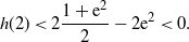 \begin{align*}h(2) < 2 \frac{1 +{\mathrm{e}}^2}{2} - 2{\mathrm{e}}^2 < 0.\end{align*}
Numerical results show that the root is given by $C \approx 1.50339538$
.
$C \approx 1.50339538$
.
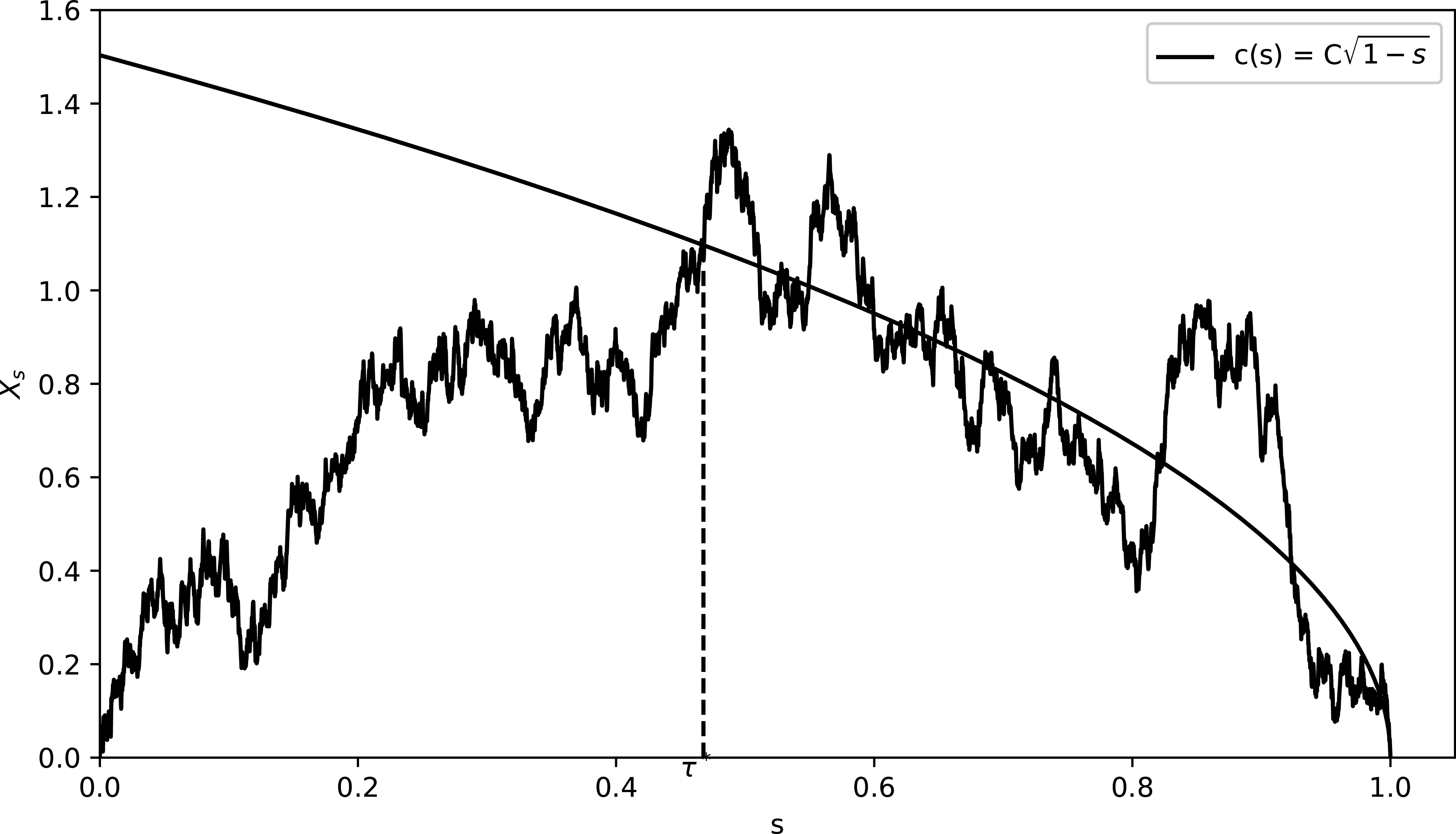
A sample path $X(\omega)= (X_t(\omega))_{0 \leq t \leq 1}$
of a Brownian excursion and the optimal stopping boundary
$X(\omega)= (X_t(\omega))_{0 \leq t \leq 1}$
of a Brownian excursion and the optimal stopping boundary $c(s)=C\sqrt{1-s}$
, where
$c(s)=C\sqrt{1-s}$
, where $C \approx 1.50339538$
. Also shown is the optimal stopping time
$C \approx 1.50339538$
. Also shown is the optimal stopping time $\tau^*(\omega) = \inf \{ u \in (0,1)\colon X_u(\omega) \geq C\sqrt{(1-u)} \}$
.
$\tau^*(\omega) = \inf \{ u \in (0,1)\colon X_u(\omega) \geq C\sqrt{(1-u)} \}$
.
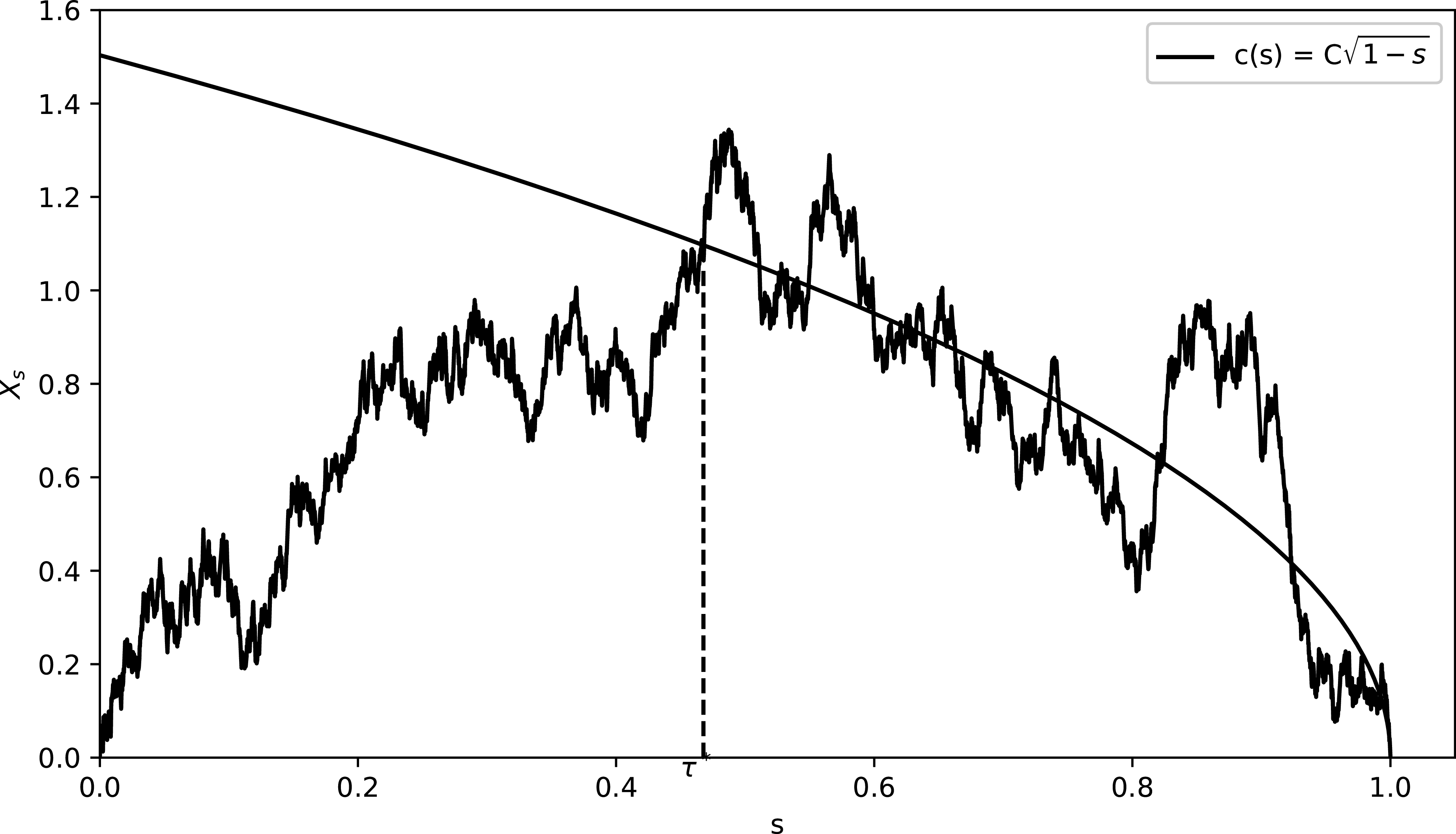
Figure 1 Long description
A line graph depicting a sample path of a Brownian excursion and the optimal stopping boundary, with the optimal stopping time marked. The x-axis represents the variable s ranging from 0 to 1, and the y-axis represents the variable X sub s ranging from 0 to 1.6. The graph includes a solid line representing the function c(s) equals C times the square root of 1 minus s. A dashed vertical line marks the optimal stopping time at approximately 0.45 on the x-axis. The sample path fluctuates around the optimal stopping boundary, showing peaks and troughs. All values are approximated.
The next result is technical and the proof is postponed to the Appendix.
Lemma 2.1. Let $f\colon [0,C] \to [0,\infty)$
be given by (2.11) with
$f\colon [0,C] \to [0,\infty)$
be given by (2.11) with $A=0$
and B given by (2.12).
$A=0$
and B given by (2.12).
Then $f(0)=B$
and
$f(0)=B$
and $f'(0)=0$
. Moreover, f is convex with
$f'(0)=0$
. Moreover, f is convex with $f\,(\,y)\geq y$
for all
$f\,(\,y)\geq y$
for all $y \in [0,C]$
.
$y \in [0,C]$
.
Putting together (2.7) with (2.11) for the choice $A=0$
and B given by (2.12) gives the candidate value function
$A=0$
and B given by (2.12) gives the candidate value function $V^*=(V^{*}(t,x))_{ (t,x) \in [0,1)\times[0,\infty) }$
:
$V^*=(V^{*}(t,x))_{ (t,x) \in [0,1)\times[0,\infty) }$
:
 \begin{equation} V^{*}(t,x)= \begin{cases} \displaystyle C^{2}\biggl(\int_{0}^{C}{\mathrm{e}}^{{{t^{2}}/{2}}}\,{\mathrm{d}} t\biggr)^{-1}\biggl(\dfrac{1-t}{x}\biggr) \int_{0}^{{{x}/{\sqrt{1-t}}}}{\mathrm{e}}^{{{t^{2}}/{2}}} \,{\mathrm{d}} t &\text{if $ x<c(t)$,} \\[9pt] x &\text{if $ x\geq c(t)$,} \end{cases}\end{equation}
where $c(t)= C\sqrt{1-t}$
and C solves (2.13). The next step is to show that the candidate value function
$c(t)= C\sqrt{1-t}$
and C solves (2.13). The next step is to show that the candidate value function $V^{*}(t,x)$
is indeed the true solution to the optimal stopping problem introduced in (2.2).
$V^{*}(t,x)$
is indeed the true solution to the optimal stopping problem introduced in (2.2).
Theorem 2.1. The candidate value function $V^{*}$
given in (2.14) coincides with the value function
$V^{*}$
given in (2.14) coincides with the value function $\bar{V}$
defined in (2.2). Moreover, the associated stopping time
$\bar{V}$
defined in (2.2). Moreover, the associated stopping time $\tau^*$
, given by
$\tau^*$
, given by
 \begin{equation*} \tau^{*}=\inf\{s\geq t\;\colon X_{s}\geq c(s)\}, \end{equation*}
where $c(s)=C\sqrt{1-s}$
and
$c(s)=C\sqrt{1-s}$
and $C \in (0,\infty)$
is the unique solution to (2.13), is optimal for the problem started at
$C \in (0,\infty)$
is the unique solution to (2.13), is optimal for the problem started at $(t,x)$
.
$(t,x)$
.
Proof. Fix $t_0 \in [0,1)$
. We show that
$t_0 \in [0,1)$
. We show that $V^{*}(t_0,x)=\bar{V}(t_0,x)$
by first proving
$V^{*}(t_0,x)=\bar{V}(t_0,x)$
by first proving $V^{*}(t_0,x)\geq \bar{V}(t_0,x)$
, and then proving the reverse inequality.
$V^{*}(t_0,x)\geq \bar{V}(t_0,x)$
, and then proving the reverse inequality.
For $t \geq t_0$
, let
$t \geq t_0$
, let $M = \{ M_t \}_{t \geq t_0}$
be given by
$M = \{ M_t \}_{t \geq t_0}$
be given by $M_{t}=V^{*}(t,X_{t})$
. Itô’s formula gives us
$M_{t}=V^{*}(t,X_{t})$
. Itô’s formula gives us
 \begin{equation*} {\mathrm{d}} M_{t}=V^{*}_{t}(t,X_{t})\,{\mathrm{d}} t+V_{x}^{*}(t,X_{t})\,{\mathrm{d}} X_{t}+\dfrac{1}{2}V_{xx}^{*}(t,X_{t})\,{\mathrm{d}} \langle X\rangle_{t}. \end{equation*}
Therefore, recalling (2.1), we find
 \begin{equation*} {\mathrm{d}} M_{t}=\biggl[V_{t}^{*}(t,X_{t})+\biggl(\dfrac{1}{X_{t}}-\dfrac{X_{t}}{1-t}\biggr)V_{x}^{*}(t,X_{t}) +\dfrac{1}{2}V_{xx}^{*}(t,X_{t})\biggr]\,{\mathrm{d}} t+V_{x}^{*}(t,X_{t})\,{\mathrm{d}} W_{t}.\end{equation*}
Since $V^{*}(t,x)$
solves (2.3) when
$V^{*}(t,x)$
solves (2.3) when $x<c(t)$
, the drift term vanishes in the continuation region, i.e.
$x<c(t)$
, the drift term vanishes in the continuation region, i.e. $X_{t}<c(t)$
. In contrast, when X is in the stopping region, i.e.
$X_{t}<c(t)$
. In contrast, when X is in the stopping region, i.e. $X_t\geq c(t)$
, we have
$X_t\geq c(t)$
, we have $V^{*}(t,x)=x$
, and the drift term simplifies. Putting the cases together,
$V^{*}(t,x)=x$
, and the drift term simplifies. Putting the cases together,
 \begin{equation} {\mathrm{d}} M_{t}= g(t,X_t)\mathbb{I}\{X_{t}\geq c(t)\}\,{\mathrm{d}} t +V_{x}^{*}(t,X_{t})\,{\mathrm{d}} W_{t},\end{equation}
where
 \begin{equation*} g(t,x)= x^{-1} \biggl( 1 -\dfrac{x^2}{1-t} \biggr).\end{equation*}
Note that for each $t \in [0,1)$
,
$t \in [0,1)$
, $g(t,\cdot)$
is decreasing in x and therefore, for every
$g(t,\cdot)$
is decreasing in x and therefore, for every $x\geq c(t)$
,
$x\geq c(t)$
, $g(t,x)\leq g(t,c(t))$
. Moreover, since
$g(t,x)\leq g(t,c(t))$
. Moreover, since $C>1$
,
$C>1$
,
 \begin{equation*} g(t,c(t))= g(t,C\sqrt{1-t})=\biggl(\dfrac{1}{C}-C\biggr)\sqrt{1-t}<0.\end{equation*}
It follows that
 \begin{align*}\int_{t_0}^\cdot \biggl(\frac{1}{X_{t}}-\frac{X_{t}}{1-t}\biggr)\mathbb{I}\{X_{t}\geq c(t)\}\,{\mathrm{d}} t\end{align*}
is a decreasing process.
The process $\int_{t_0}^\cdot V^{*}_{x}\,{\mathrm{d}} W_{t}$
is a local martingale: we want to argue that
$\int_{t_0}^\cdot V^{*}_{x}\,{\mathrm{d}} W_{t}$
is a local martingale: we want to argue that $\int_{t_0}^{\cdot}V^{*}_{x}(s,X_s)\,{\mathrm{d}} W_{s}$
is a martingale. This will follow if
$\int_{t_0}^{\cdot}V^{*}_{x}(s,X_s)\,{\mathrm{d}} W_{s}$
is a martingale. This will follow if $V^*_x$
is bounded, and in the stopping region this is immediate since
$V^*_x$
is bounded, and in the stopping region this is immediate since $V^*_x \equiv 1$
. In the continuation region we have
$V^*_x \equiv 1$
. In the continuation region we have
 \begin{align*}V^{*}(t,x) = \sqrt{1-t}\,f\biggl(\frac{x}{\sqrt{1-t}}\biggr){,}\end{align*}
where
 \begin{align*} f\,(\,y)= \frac{B}{y}\int_{0}^{y}{\mathrm{e}}^{{{t^{2}}/{2}}}\,{\mathrm{d}} t\end{align*}
and B and C are given in (2.12) and (2.13). Then
 \begin{align*}V^{*}_{x}(t,x) \,=\, f' \biggl(\frac{x}{\sqrt{1-t}}\biggr).\end{align*}
From Lemma 2.1 we conclude that f is a convex function, and thus $f' \in [f'(0),f'(C)]=[0,1]$
on [0, C]. Hence
$f' \in [f'(0),f'(C)]=[0,1]$
on [0, C]. Hence $V_{x}^{*}=f'$
is bounded, and
$V_{x}^{*}=f'$
is bounded, and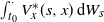 $\int_{t_0}^\cdot V_{x}^{*}(s,x)\,{\mathrm{d}} W_{s}$
is a martingale.
$\int_{t_0}^\cdot V_{x}^{*}(s,x)\,{\mathrm{d}} W_{s}$
is a martingale.
Putting together the results of the last paragraph, $M=\{M_{t}\}_{t\geq t_0}$
is a supermartingale. Moreover,
$M=\{M_{t}\}_{t\geq t_0}$
is a supermartingale. Moreover, $V^*(t,x) \geq x$
; this follows by definition on
$V^*(t,x) \geq x$
; this follows by definition on $x \geq c(t)$
and from Lemma 2.1 on the continuation region. Then
$x \geq c(t)$
and from Lemma 2.1 on the continuation region. Then $\mathbb{E}_{t_0,x}[X_\tau] \leq \mathbb{E}_{t_0,x}[V^*(\tau,X_\tau)]$
. Further, by the Optional Stopping Theorem,
$\mathbb{E}_{t_0,x}[X_\tau] \leq \mathbb{E}_{t_0,x}[V^*(\tau,X_\tau)]$
. Further, by the Optional Stopping Theorem, $\mathbb{E}_{t_0,x}[V^{*}(\tau,X_{\tau})]\leq V^{*}(t_0,x)$
, and then for any stopping time
$\mathbb{E}_{t_0,x}[V^{*}(\tau,X_{\tau})]\leq V^{*}(t_0,x)$
, and then for any stopping time $\tau$
taking values in
$\tau$
taking values in $[t_0,1]$
,
$[t_0,1]$
, $ \mathbb{E}_{t_0,x}[X_{\tau}]\leq \mathbb{E}_{t_0,x}[V^{*}(\tau,X_{\tau})]\leq V^{*}(t_0,x).$
It follows that
$ \mathbb{E}_{t_0,x}[X_{\tau}]\leq \mathbb{E}_{t_0,x}[V^{*}(\tau,X_{\tau})]\leq V^{*}(t_0,x).$
It follows that
 \begin{equation} \bar{V}(t_0,x)=\sup\nolimits_{t_0 \leq \tau \leq 1}\mathbb{E}_{t_0,x}[X_{\tau}]\leq V^{*}(t_0,x).\end{equation}
Now we show the reverse inequality $\bar{V}(t_0,x) \geq V^*(t_0,x)$
. If
$\bar{V}(t_0,x) \geq V^*(t_0,x)$
. If $X_{t_0} \geq c(t_0)$
, then taking
$X_{t_0} \geq c(t_0)$
, then taking $\tau = t_0$
we have
$\tau = t_0$
we have $\bar{V}(t_0,x) \geq x = V^*(t_0,x)$
. It remains to consider the case
$\bar{V}(t_0,x) \geq x = V^*(t_0,x)$
. It remains to consider the case $X_{t_0} < c(t_0)$
. Set
$X_{t_0} < c(t_0)$
. Set $\tau^{*} = \inf\{s\geq t_0\colon X_{s}\geq c(s)\}$
. It follows that
$\tau^{*} = \inf\{s\geq t_0\colon X_{s}\geq c(s)\}$
. It follows that $X_{t\wedge\tau^{*}}\leq c(t)$
almost surely. Then from (2.15) we conclude that
$X_{t\wedge\tau^{*}}\leq c(t)$
almost surely. Then from (2.15) we conclude that $V^{*}(t\wedge \tau^*,X_{t\wedge\tau^{*}})$
is a martingale. Using the Optional Stopping Theorem again, we have
$V^{*}(t\wedge \tau^*,X_{t\wedge\tau^{*}})$
is a martingale. Using the Optional Stopping Theorem again, we have
 \begin{align*}V^{*}(t_0,x)=\mathbb{E}_{t_0,x}[V^{*}(\tau^{*},X_{\tau^{*}})]=\mathbb{E}_{t,x}[X_{\tau^{*}}]{,}\end{align*}
where the second equality comes from the fact that $V^{*}(t,c(t))=c(t)$
. Hence
$V^{*}(t,c(t))=c(t)$
. Hence
 \begin{equation*} \bar{V}(t_0,x)=\sup\nolimits_{t_0 \leq \tau \leq 1}\mathbb{E}_{t_0,x}[X_{\tau}]\geq \mathbb{E}_{t_0,x}[X_{\tau^{*}}]= V^{*}(t_0,x).\end{equation*}
Combining this result with (2.16), we have $\bar{V}(t_0,x) = V^*(t_0,x)$
, and
$\bar{V}(t_0,x) = V^*(t_0,x)$
, and $\tau^*$
is optimal.
$\tau^*$
is optimal.
3. Optimal stopping of an $\alpha$
-dimensional Bessel bridge
$\alpha$
-dimensional Bessel bridge

A Brownian excursion can also be viewed as a three-dimensional Bessel bridge. In this section we are interested in extending the problem of Section 2 to allow for an $\alpha$
-dimensional Bessel bridge as the underlying stochastic process, and to include more general objective functions of power law form.
$\alpha$
-dimensional Bessel bridge as the underlying stochastic process, and to include more general objective functions of power law form.
At least when $\alpha$
is an integer, the
$\alpha$
is an integer, the $\alpha$
-dimensional Bessel process corresponds to the radial part of
$\alpha$
-dimensional Bessel process corresponds to the radial part of $\alpha$
-dimensional Brownian motion. For
$\alpha$
-dimensional Brownian motion. For $\alpha\geq 2$
,
$\alpha\geq 2$
, $\alpha$
-dimensional Brownian motion started at the origin never returns to zero. Correspondingly, an
$\alpha$
-dimensional Brownian motion started at the origin never returns to zero. Correspondingly, an $\alpha$
-dimensional Bessel process started at the origin never hits zero after time zero (provided
$\alpha$
-dimensional Bessel process started at the origin never hits zero after time zero (provided $\alpha \geq 2$
). Similarly, when
$\alpha \geq 2$
). Similarly, when $\alpha\geq 2$
, an
$\alpha\geq 2$
, an $\alpha$
-dimensional Bessel bridge is strictly positive on time-interval (0, 1). However, for
$\alpha$
-dimensional Bessel bridge is strictly positive on time-interval (0, 1). However, for $\alpha \in (0,2)$
, both an
$\alpha \in (0,2)$
, both an $\alpha$
-dimensional Bessel process and an
$\alpha$
-dimensional Bessel process and an $\alpha$
-dimensional Bessel bridge return to zero countably many times in (0, 1), as well as at time 1 for the Bessel bridge. This can cause complications in the study of the Bessel process; for example, when
$\alpha$
-dimensional Bessel bridge return to zero countably many times in (0, 1), as well as at time 1 for the Bessel bridge. This can cause complications in the study of the Bessel process; for example, when $0 < \alpha < 1$
the
$0 < \alpha < 1$
the $\alpha$
-dimensional Bessel process does not have a representation via a stochastic differential equation. Instead we work with the squared Bessel process, and the squared Bessel bridge. Bessel processes and squared Bessel processes are discussed in detail in Revuz and Yor [Reference Revuz and Yor9]; see Chapter 11 and especially Exercise 3.11.
$\alpha$
-dimensional Bessel process does not have a representation via a stochastic differential equation. Instead we work with the squared Bessel process, and the squared Bessel bridge. Bessel processes and squared Bessel processes are discussed in detail in Revuz and Yor [Reference Revuz and Yor9]; see Chapter 11 and especially Exercise 3.11.
Definition 3.1. Suppose $\alpha>0$
. A non-negative continuous process
$\alpha>0$
. A non-negative continuous process $Q=\{Q_{t}\}_{0\leq t\leq 1}$
is an
$Q=\{Q_{t}\}_{0\leq t\leq 1}$
is an $\alpha$
-dimensional squared Bessel bridge process if it satisfies the SDE
$\alpha$
-dimensional squared Bessel bridge process if it satisfies the SDE
 \begin{equation*} {\mathrm{d}} Q_{t}=\biggl(\alpha - \dfrac{2Q_{t}}{1-t} \biggr)\,{\mathrm{d}} t+ 2 \sqrt{Q}_t \,{\mathrm{d}} W_{t}, \quad 0<t<1, \end{equation*}
subject to $Q_0=0$
.
$Q_0=0$
.
Remark 3.1. Given a process Q as in Definition 3.1, we can define an $\alpha$
-dimensional Bessel bridge
$\alpha$
-dimensional Bessel bridge $X= (X_t)_{0 \leq t \leq 1}$
by
$X= (X_t)_{0 \leq t \leq 1}$
by $X_t = \sqrt{Q_t}$
. If
$X_t = \sqrt{Q_t}$
. If $\alpha \geq 2$
so that
$\alpha \geq 2$
so that $Q>0$
on (0, 1), we can apply Itô’s formula to deduce that X solves the SDE
$Q>0$
on (0, 1), we can apply Itô’s formula to deduce that X solves the SDE
 \begin{align*}{\mathrm{d}} X_t = \biggl( \frac{\alpha-1}{2X_t} - \frac{X_t}{1-t} \biggr) \,{\mathrm{d}} t + {\mathrm{d}} W_t,\end{align*}
and when $\alpha=3$
we recognize the Brownian excursion of Definition 2.1. When
$\alpha=3$
we recognize the Brownian excursion of Definition 2.1. When $\alpha \geq 2$
we can continue to work with this representation, but when
$\alpha \geq 2$
we can continue to work with this representation, but when $\alpha \in [1,2)$
we need to deal with the times when
$\alpha \in [1,2)$
we need to deal with the times when $X=0$
, and when
$X=0$
, and when $\alpha \in (0,1)$
, X cannot be written as the solution of an SDE, hence our re-specification of the problem via the squared Bessel process.
$\alpha \in (0,1)$
, X cannot be written as the solution of an SDE, hence our re-specification of the problem via the squared Bessel process.
Our goal is to investigate the optimal stopping problem for the $\alpha$
-dimensional Bessel bridge with power-law payoff
$\alpha$
-dimensional Bessel bridge with power-law payoff $\phi(x)=x^n$
. For
$\phi(x)=x^n$
. For $\alpha \in (0,\infty)$
and
$\alpha \in (0,\infty)$
and $n \in (0,\infty)$
, define
$n \in (0,\infty)$
, define $\bar{V}(t,x)=\sup_{t\leq\tau\leq 1}\mathbb{E}_{t,x}[X_{\tau}^{n}]$
. Then
$\bar{V}(t,x)=\sup_{t\leq\tau\leq 1}\mathbb{E}_{t,x}[X_{\tau}^{n}]$
. Then $\bar{V}(t,x)=\bar{U}(t,x^2)$
, where
$\bar{V}(t,x)=\bar{U}(t,x^2)$
, where
 \begin{equation} \bar{U}(t,q)=\sup\nolimits_{t\leq\tau\leq 1}\mathbb{E}_{t,q}[Q_{\tau}^{n/2}],\end{equation}
where Q is the squared Bessel bridge introduced in Definition 3.1. As in the last section, we aim to find the optimal stopping time $\tau^{*}$
in which the supremum in (3.1) is attained. For the problem started at time
$\tau^{*}$
in which the supremum in (3.1) is attained. For the problem started at time $t_0 \in (0,1)$
we expect the optimal stopping rule to be of threshold form,
$t_0 \in (0,1)$
we expect the optimal stopping rule to be of threshold form,
 \begin{equation*} \tau^{*}=\inf\{s\geq t_0\colon X_{s}\geq \sqrt{z(s)} \} = \inf\{s\geq t_0\colon Q_{s}\geq z(s)\},\end{equation*}
where $z(\!\cdot\!)$
is the optimal boundary (for the squared Bessel bridge). Following the Brownian excursion case, in the continuation region
$z(\!\cdot\!)$
is the optimal boundary (for the squared Bessel bridge). Following the Brownian excursion case, in the continuation region $\mathcal{C}_Q =\{ (t,q) \subseteq [0,1) \times [0,z(t)) \}$
we have that for a candidate solution
$\mathcal{C}_Q =\{ (t,q) \subseteq [0,1) \times [0,z(t)) \}$
we have that for a candidate solution $U=(U(t,q))_{ (t,q) \in [0,1) \times [0,\infty)}$
,
$U=(U(t,q))_{ (t,q) \in [0,1) \times [0,\infty)}$
,
 \begin{equation*} {\mathrm{d}} U(t, Q_{t})=\biggl[U_{t}(t,Q_{t}) +U_{q}(t,Q_{t})\biggl(\alpha-\dfrac{2Q_{t}}{1-t}\biggr) +2 Q_t U_{qq}(t, Q_{t})\biggr]\,{\mathrm{d}} t+ 2 \sqrt{Q_t} U_{q}(t,Q_{t})\,{\mathrm{d}} W_{t},\end{equation*}
and on ${\mathcal C}_Q$
we expect that U solves the PDE
${\mathcal C}_Q$
we expect that U solves the PDE
 \begin{equation} U_{t}(t,q) +\biggl(\alpha-\dfrac{2q}{1-t}\biggr)U_{q}(t,q) + 2q U_{qq}(t, q) = 0 \end{equation}
subject to
 \begin{align*}U(t,z(t))= z(t)^{n/2}\quad\text{and}\quad U_{q}(t,z(t))= \frac{n}{2} z(t)^{{{n}/{2}}-1}.\end{align*}
We make the ansatz $z(t)=Z(1-t)$
for
$z(t)=Z(1-t)$
for $Z \in (0,\infty)$
a positive constant (so that
$Z \in (0,\infty)$
a positive constant (so that $Z(1-t)$
is a downward sloping straight line passing through (1, 0)) and
$Z(1-t)$
is a downward sloping straight line passing through (1, 0)) and
 \begin{align*}V(t,x)=(1-t)^{{{n}/{2}}}f\biggl(\frac{x}{\sqrt{1-t}}\biggr){,}\end{align*}
or equivalently
 \begin{equation} U(t,q) = (1-t)^{{{n}/{2}}}g\biggl(\dfrac{q}{1-t}\biggr)\end{equation}
where f, g are functions to be determined such that $f(x)=g(x^2)$
. On
$f(x)=g(x^2)$
. On $[0,\sqrt{Z}]$
we have that f solves the ODE
$[0,\sqrt{Z}]$
we have that f solves the ODE $ y\,f''(\,y)+(\alpha-1-y^{2})\,f'(y)-n\,y\,f\,(\,y)=0, $
subject to
$ y\,f''(\,y)+(\alpha-1-y^{2})\,f'(y)-n\,y\,f\,(\,y)=0, $
subject to $ f(\sqrt{Z}) = Z^{n/2}, f'(\sqrt{Z})=nZ^{(n-1)/2},$
which is equivalent to
$ f(\sqrt{Z}) = Z^{n/2}, f'(\sqrt{Z})=nZ^{(n-1)/2},$
which is equivalent to
 \begin{equation} 4yg''(y)+ 2(\alpha-y)g'(y)-ng(y)=0, \end{equation}
subject to
 \begin{align*}g(Z) = Z^{n/2}\quad\text{and}\quad g'(Z) = \frac{n}{2}Z^{{{n}/{2}}-1}.\end{align*}
In general there does not seem to be a closed-form solution to (3.4), so we look for a solution in the form of a power series expansion. However, as well as the Brownian excursion with linear payoff $(\alpha=3,n=1)$
, there are other cases where we have explicit solutions, and before moving on to the general case we record those here.
$(\alpha=3,n=1)$
, there are other cases where we have explicit solutions, and before moving on to the general case we record those here.
Motivated by the Brownian excursion example, consider $G(y) = y^\theta$
. Then G solves (3.4) provided
$G(y) = y^\theta$
. Then G solves (3.4) provided $2\theta(\theta-1) + \alpha \theta = 0$
and
$2\theta(\theta-1) + \alpha \theta = 0$
and $-2 \theta - n=0$
. Ruling out the case
$-2 \theta - n=0$
. Ruling out the case $\theta=0$
, we find that G is a solution provided
$\theta=0$
, we find that G is a solution provided $n = - 2 \theta = \alpha-2$
, so that there is an explicit solution if
$n = - 2 \theta = \alpha-2$
, so that there is an explicit solution if $n=\alpha-2$
and then the solution is given by
$n=\alpha-2$
and then the solution is given by $G(y) = y^{-{{n}/{2}}}$
. This solution explodes at 0, but we can find another solution H of the form
$G(y) = y^{-{{n}/{2}}}$
. This solution explodes at 0, but we can find another solution H of the form
 \begin{align*} H(y) = y^{-{{n}/{2}}} \int_0^y {\mathrm{e}}^{{{s}/{2}}} s^{{{n}/{2}}-1} \dfrac{{\mathrm{d}} s}{2} = y^{1-{{\alpha}/{2}}} \int_0^y {\mathrm{e}}^{{{s}/{2}}} s^{{{\alpha}/{2}}-2} \dfrac{{\mathrm{d}} s}{2}, \quad n = \alpha - 2, \end{align*}
for which H and H ′ are strictly positive and bounded at zero. Choosing an appropriate multiple of H, we can construct a solution to (3.4) which can be used as the basis for the candidate solution of the optimal stopping problem.
Another example from the literature where an explicit solution is known is the case of a reflecting Brownian bridge ( $\alpha=1,n=1$
); see Ekström and Wanntorp [Reference Ekström and Wanntorp5]. In this case
$\alpha=1,n=1$
); see Ekström and Wanntorp [Reference Ekström and Wanntorp5]. In this case $G(y)= {\mathrm{e}}^{{y}/{2}}$
solves (3.4). Motivated by this example, consider
$G(y)= {\mathrm{e}}^{{y}/{2}}$
solves (3.4). Motivated by this example, consider $G(y) = y^\theta {\mathrm{e}}^{y/2}$
. We find that G solves (3.4) provided either
$G(y) = y^\theta {\mathrm{e}}^{y/2}$
. We find that G solves (3.4) provided either $(\theta=0,\alpha=n)$
or
$(\theta=0,\alpha=n)$
or $(n=2,\alpha=2 - 2\theta)$
. In particular, when
$(n=2,\alpha=2 - 2\theta)$
. In particular, when $\alpha=n$
we find that the candidate value function is given by
$\alpha=n$
we find that the candidate value function is given by
 \begin{align*}{U(t,q)=(1-t)^{n/2} n^{n/2}\exp\biggl({\frac{(q-\sqrt{n})}{2(1-t)}}\biggr)\quad\text{and}\quad Z=\sqrt{n}.}\end{align*}
For the Brownian bridge we recover that the candidate value function is
 \begin{align*}V^*(t,x) = (1-t)^{1/2}\exp\biggl({\frac{x^2-1}{2(1-t)}}\biggr)\end{align*}
and the candidate optimal stopping rule is $\tau^* = \inf \{ t \geq t_0 \colon X_t \geq \sqrt{1-t} \}$
. Further, when
$\tau^* = \inf \{ t \geq t_0 \colon X_t \geq \sqrt{1-t} \}$
. Further, when $n=2$
, we find that
$n=2$
, we find that $G(y)= y^{1 - {{\alpha}/{2}}} {\mathrm{e}}^{y/2}$
is a solution to (3.4), and the candidate value function (at least when
$G(y)= y^{1 - {{\alpha}/{2}}} {\mathrm{e}}^{y/2}$
is a solution to (3.4), and the candidate value function (at least when $\alpha>2$
) is built from the second solution to (3.4),
$\alpha>2$
) is built from the second solution to (3.4),
 \begin{align*} H(y) = E y^{1- \alpha/2} {\mathrm{e}}^{y/2} \int_0^y {\mathrm{e}}^{-v/2} v^{-2 + {{\alpha}/{2}}} \dfrac{{\mathrm{d}} v}{2} \end{align*}
for some constant $E>0$
.
$E>0$
.
Returning to the general case, we look for a solution in power series form. Let $\psi(y)=\sum_{k=0}^{\infty}A_{k}y^{k}$
, where
$\psi(y)=\sum_{k=0}^{\infty}A_{k}y^{k}$
, where $A_0=1$
so that
$A_0=1$
so that $\psi(0)=1$
. Then we have
$\psi(0)=1$
. Then we have
 \begin{align*}\psi'(y)=\sum_{k=1}^{\infty}k\,A_{k}y^{k-1}\quad\text{and}\quad \psi''(y)=\sum_{k=2}^{\infty}k(k-1)A_{k}y^{k-2}.\end{align*}
Substituting these back into (3.4), we obtain a recursive equation for the coefficients $(A_k)_{k \geq 0}$
,
$(A_k)_{k \geq 0}$
,
 \begin{equation*}A_{k+1}=\dfrac{(2k+n)}{2(k+1)(2k+\alpha)} A_k, \quad A_0=1, \end{equation*}
which has solution
 \begin{equation} A_{k}=\dfrac{\Gamma({{\alpha}/{2}})}{\Gamma({{n}/{2}})}\dfrac{\Gamma(k+{{n}/{2}})}{\Gamma(k+{{\alpha}/{2}})2^{k}k!},\end{equation}
where $\Gamma$
is the Gamma function defined as
$\Gamma$
is the Gamma function defined as
 \begin{align*}\Gamma(z)=\int_{0}^{\infty}{\mathrm{e}}^{-x}x^{z-1}\,{\mathrm{d}} x.\end{align*}
Given $\psi$
, we can define a second solution
$\psi$
, we can define a second solution $\psi_2$
to (3.4) of the form
$\psi_2$
to (3.4) of the form
 \begin{align*} \psi_2(y) = \psi(y) \int_0^y \dfrac{ s^{-\alpha/2} {\mathrm{e}}^{s/2} }{\psi(s)^{2}} \dfrac{{\mathrm{d}} s}{2}, \end{align*}
and the general solution to (3.4) is
 \begin{equation}g(y) = E_1 \psi(y) + E_2 \psi_2(y).\end{equation}
Note that $\psi_2(y) \sim y^{1- \alpha/2}$
for small y. We want a solution for which g
′ is bounded on [0, Z] and g
″ is finite at 0 and for which the boundary conditions hold at Z. Together, the first set of conditions implies that
$\psi_2(y) \sim y^{1- \alpha/2}$
for small y. We want a solution for which g
′ is bounded on [0, Z] and g
″ is finite at 0 and for which the boundary conditions hold at Z. Together, the first set of conditions implies that $E_2=0$
and the boundary conditions at Z imply that Z solves
$E_2=0$
and the boundary conditions at Z imply that Z solves $Z \psi'(Z) = ({{n}/{2}}) \psi(Z)$
. This is equivalent to
$Z \psi'(Z) = ({{n}/{2}}) \psi(Z)$
. This is equivalent to $F_{\alpha,n} (Z)=0$
, where
$F_{\alpha,n} (Z)=0$
, where
 \begin{equation} F_{\alpha,n}(z) = \sum_{k=0}^{\infty} (2k-n)A_{k}z^{k}.\end{equation}
The next result follows from Lemma A.1 in the Appendix.
An example of $F_{\alpha,n}(z)$
, where
$F_{\alpha,n}(z)$
, where $\alpha=3$
and
$\alpha=3$
and $n=2$
, and its corresponding root
$n=2$
, and its corresponding root $Z_{3,2}$
, which satisfies
$Z_{3,2}$
, which satisfies $Z_{3,2}> {{(3+2-2)}/{2}}=1.5$
. Note that the figure confirms the results in Corollary 3.1 and Proposition 3.1 for this parameter combination; the issue is to prove these results for general parameters.
$Z_{3,2}> {{(3+2-2)}/{2}}=1.5$
. Note that the figure confirms the results in Corollary 3.1 and Proposition 3.1 for this parameter combination; the issue is to prove these results for general parameters.
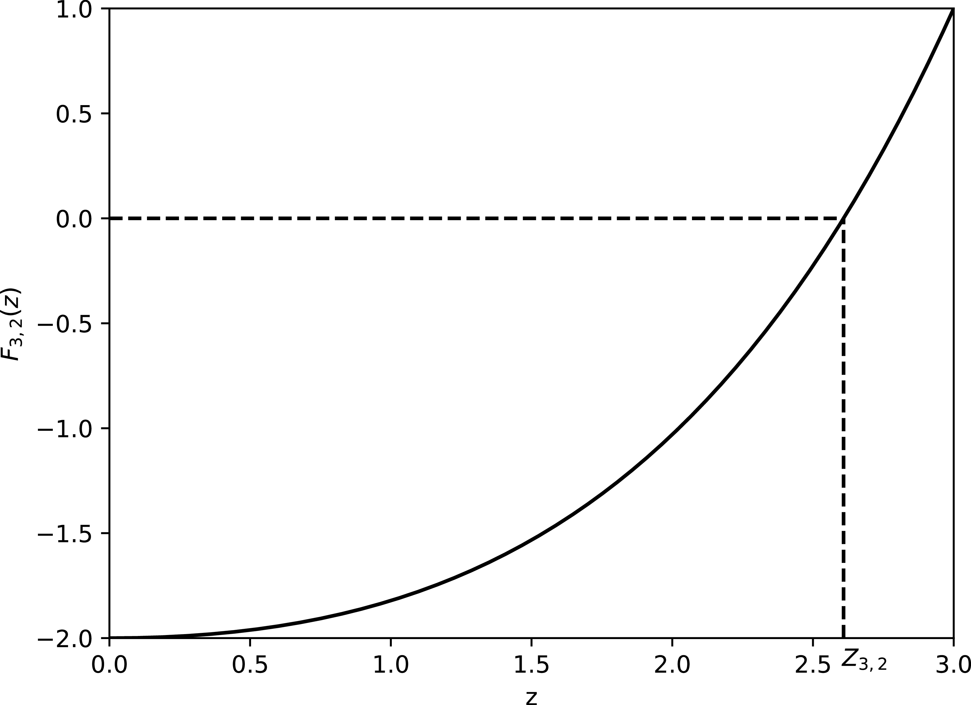
Figure 2 Long description
A line graph showing the function F subscript 3, 2 (z) with z on the x axis ranging from 0 to 3 and F subscript 3, 2 (z) on the y axis ranging from -2 to 1. The graph depicts a curve that starts at -2 on the y axis and gradually increases, crossing the x axis at approximately z equals 2.5. A dashed horizontal line is present at y equals 0, and a dashed vertical line is present at z equals 2.5, indicating the root of the function. All values are approximated.
Corollary 3.1. $F_{\alpha,n}$
has a unique positive root
$F_{\alpha,n}$
has a unique positive root $Z = Z_{\alpha,n}$
. Moreover,
$Z = Z_{\alpha,n}$
. Moreover, $F_{\alpha,n}(z) < 0$
on
$F_{\alpha,n}(z) < 0$
on $[0,Z_{\alpha,n})$
.
$[0,Z_{\alpha,n})$
.
Recall that the root $Z_{\alpha,n}$
defines the candidate optimal boundary to the optimal stopping problem for the
$Z_{\alpha,n}$
defines the candidate optimal boundary to the optimal stopping problem for the $\alpha$
-dimensional squared Bessel process with payoff
$\alpha$
-dimensional squared Bessel process with payoff $\phi(q) = q^{n/2}$
via
$\phi(q) = q^{n/2}$
via $\tau^* = \inf \{ t \in (0,1) \colon Q_t \geq Z(1-t) \}.$
Moreover, the coefficient
$\tau^* = \inf \{ t \in (0,1) \colon Q_t \geq Z(1-t) \}.$
Moreover, the coefficient $E_1$
in (3.6) can be computed using
$E_1$
in (3.6) can be computed using $Z^{n/2} = g(Z) = E_1 \psi(Z)$
to give
$Z^{n/2} = g(Z) = E_1 \psi(Z)$
to give
 \begin{equation*} E_1 = \dfrac{Z_{\alpha,n}^{n/2}}{\sum_{k=0}^{\infty}A_{k}Z_{\alpha,n}^{k}}.\end{equation*}
Therefore we can define a candidate value function $U^*$
using (3.3) and (3.6) of the form
$U^*$
using (3.3) and (3.6) of the form
 \begin{equation} U^{*}(t,q)= \begin{cases} \biggl(\dfrac{Z_{\alpha,n}^{n/2}}{\sum_{k=0}^{\infty}A_{k}Z_{\alpha,n}^{k}}\biggr)(1-t)^{{{n}/{2}}}\sum_{k=0}^{\infty}A_{k}\biggl(\dfrac{q}{{1-t}}\biggr)^{k} & \text{if $ q < Z_{\alpha,n} (1-t)$,}\\[9pt] q^{n/2} &\text{if $ q \geq Z_{\alpha,n} (1-t) $,}\end{cases}\end{equation}
where $(A_{k})_{k \geq 0}$
are given by (3.5) and
$(A_{k})_{k \geq 0}$
are given by (3.5) and $Z_{\alpha,n}$
is the unique solution to (3.7).
$Z_{\alpha,n}$
is the unique solution to (3.7).
Recall that $g(y) = E_1 \psi(y) = E_1 \sum_{k \geq 0} A_k y^k$
on [0, Z].
$g(y) = E_1 \psi(y) = E_1 \sum_{k \geq 0} A_k y^k$
on [0, Z].
Lemma 3.1. For $z \in [0,Z]$
we have
$z \in [0,Z]$
we have $g(z) \geq z^{n/2}$
.
$g(z) \geq z^{n/2}$
.
Proof. We have
 \begin{align*}2y g'(y) - ng(y) = \frac{E_1}{2}F_{\alpha,n}(y) < 0\ \text{on [0, ${Z}$).}\end{align*}
Then, for $z \in (0,Z)$
, we have
$z \in (0,Z)$
, we have
 \begin{align*}\ln \frac{g(Z)}{g(z)} = \int_z^Z \frac{g'(y)}{g(y)} \,{\mathrm{d}} y < \frac{n}{2} \int_z^Z \frac{1}{y}\,{\mathrm{d}} y = \ln \frac{Z^{n/2}}{z^{n/2}}{,}\end{align*}
and then using $g(Z) = Z^{n/2}$
we find
$g(Z) = Z^{n/2}$
we find $g(z) \geq z^{n/2}$
on
$g(z) \geq z^{n/2}$
on $[0,Z]$
.
$[0,Z]$
.
The next result is important for the main theorem. However, the proof is long and intricate and so it is postponed to the Appendix. Note that when $\alpha+n \leq 2$
there is nothing to prove.
$\alpha+n \leq 2$
there is nothing to prove.
Proposition 3.1. For every $\alpha > 0$
and
$\alpha > 0$
and $n>0$
, the root
$n>0$
, the root $Z_{\alpha,n} \in (0,\infty)$
to
$Z_{\alpha,n} \in (0,\infty)$
to $F_{\alpha,n}(\!\cdot\!)=0$
is such that
$F_{\alpha,n}(\!\cdot\!)=0$
is such that $Z_{\alpha,n}\geq {{(\alpha+n-2)}/{2}}$
.
$Z_{\alpha,n}\geq {{(\alpha+n-2)}/{2}}$
.
Theorem 3.1. The candidate value function $U^{*}$
given in (3.8) coincides with the value function
$U^{*}$
given in (3.8) coincides with the value function $\bar{U}$
defined in (3.1). Moreover, the associated stopping time
$\bar{U}$
defined in (3.1). Moreover, the associated stopping time $\tau^*$
given by
$\tau^*$
given by
 \begin{equation*} \tau^{*}=\inf\{s\geq t\colon Q_{s}\geq z(s) \}, \end{equation*}
where $z(s)=Z_{\alpha,n}(1-s)$
and
$z(s)=Z_{\alpha,n}(1-s)$
and $Z_{\alpha,n}$
is the root given in Corollary 3.1, is optimal for the problem started at
$Z_{\alpha,n}$
is the root given in Corollary 3.1, is optimal for the problem started at $(t,x)$
.
$(t,x)$
.
Proof. The proof follows the proof of Theorem 2.1 and here we only describe the necessary changes.
Fix $t_0$
, and for
$t_0$
, and for $t \geq t_0$
let
$t \geq t_0$
let $M_{t}=U^{*}(t,Q_{t})$
. Recall that we chose a power series expansion such that g, g
′, and g
″ are all well-defined at 0. Hence
$M_{t}=U^{*}(t,Q_{t})$
. Recall that we chose a power series expansion such that g, g
′, and g
″ are all well-defined at 0. Hence $U^*_q$
is bounded on [0, Z] and
$U^*_q$
is bounded on [0, Z] and $U^*_{qq}$
exists on [0, Z) so that we can apply Itô’s formula. We have
$U^*_{qq}$
exists on [0, Z) so that we can apply Itô’s formula. We have
 \begin{equation*} {\mathrm{d}} M_{t}= h(t,Q_t)\mathbb{I}\{Q_{t}\geq z(t) \}\,{\mathrm{d}} t +U_{q}^{*}(t,Q_{t}) 2 \sqrt{Q_t} \,{\mathrm{d}} W_{t},\end{equation*}
where
 \begin{equation*} h(t,q)= n q^{{{n}/{2}}-1}\biggl( \dfrac{\alpha + n - 2}{2} - \dfrac{q}{1-t}\biggr).\end{equation*}
Since $Z_{\alpha,n} \geq {{(\alpha+n-2)}/{2}}$
, we deduce that
$Z_{\alpha,n} \geq {{(\alpha+n-2)}/{2}}$
, we deduce that $h \leq 0$
on the stopping region
$h \leq 0$
on the stopping region $Q_t \geq Z_{\alpha,n} (1-t)$
. It follows that
$Q_t \geq Z_{\alpha,n} (1-t)$
. It follows that $A = \{ A_t \}_{t_0 \leq t \leq 1}$
given by
$A = \{ A_t \}_{t_0 \leq t \leq 1}$
given by
 \begin{align*}A_{t}\;:\!=\; \int_{t_0}^{t}h(s,Q_{s})\mathbb{I}\{Q_{s}\geq z(s)\}\,{\mathrm{d}} s\end{align*}
is a decreasing process, null at $t_0$
.
$t_0$
.
Define the local martingale $N= \{ N_t \}_{t_0 \leq t \leq 1}$
by
$N= \{ N_t \}_{t_0 \leq t \leq 1}$
by
 \begin{align*}N_{t}=\int_{t_0}^{t}U^{*}(s,Q_{s}) 2 \sqrt{Q_s} \,{\mathrm{d}} W_{s}.\end{align*}
Then $M_t = U^*(t_0,Q_{t_0}) + A_t +N_t$
. Since
$M_t = U^*(t_0,Q_{t_0}) + A_t +N_t$
. Since $M \geq 0$
, we have
$M \geq 0$
, we have $N \geq -U^*(t_0,Q_{t_0})-A_t \geq -U^*(t_0,Q_{t_0})$
and therefore the local martingale N is bounded below. Hence N is a supermartingale. It follows that
$N \geq -U^*(t_0,Q_{t_0})-A_t \geq -U^*(t_0,Q_{t_0})$
and therefore the local martingale N is bounded below. Hence N is a supermartingale. It follows that
 \begin{align*}\mathbb{E}[M_{t}\mid \mathcal{F}_{s}]=U^*(t_0,Q_{t_0}) + \mathbb{E}[A_{t}+N_{t}\mid \mathcal{F}_{s}] \leq U^*(t_0,Q_{t_0}) + A_{s}+ N_{s}=M_{s}\end{align*}
so that M is a supermartingale. By Lemma 3.1, $g(z) \geq z^{n/2}$
on [0, Z] and hence
$g(z) \geq z^{n/2}$
on [0, Z] and hence $U^*(t,Q_t) \geq Q_t^{n/2}$
on
$U^*(t,Q_t) \geq Q_t^{n/2}$
on $[0,\infty)$
, and it follows that for any stopping time
$[0,\infty)$
, and it follows that for any stopping time $\tau$
with
$\tau$
with $\tau \geq t_0$
,
$\tau \geq t_0$
,
 \begin{align*} \mathbb{E}_{t_0,x}[Q_\tau^{n/2}] \leq \mathbb{E}_{t_0,x} [U^*(\tau,Q_\tau)] \leq M_{t_0} = U^*(t_0,Q_{t_0}) .\end{align*}
Thus $\bar{U}(t_0,q) \leq U^*(t_0,q)$
.
$\bar{U}(t_0,q) \leq U^*(t_0,q)$
.
The remaining details which show that M is a martingale for $t_0 \leq t \leq \tau^*$
and hence that
$t_0 \leq t \leq \tau^*$
and hence that $\bar{U}(t_0,q) \geq U^*(t_0,q)$
follow exactly as in Theorem 2.1, using that
$\bar{U}(t_0,q) \geq U^*(t_0,q)$
follow exactly as in Theorem 2.1, using that $\sqrt{y}g'(y)$
is bounded on [0, Z] for our chosen g.
$\sqrt{y}g'(y)$
is bounded on [0, Z] for our chosen g.
Appendix Proofs of key results
Proof of Lemma 2.1. Recall that f is given by
 \begin{align*}f\,(\,y)= \frac{B}{y} \int_0^y {\mathrm{e}}^{{{t^2}/{2}}} \,{\mathrm{d}} t.\end{align*}
By l’Hôpital’s rule we have $f(0)=B$
. Also
$f(0)=B$
. Also
 \begin{align*}f'(y)= \frac{1}{y} \bigl(B{\mathrm{e}}^{y^2/2} - f\,(\,y)\bigr),\end{align*}
and again by l’Hôpital’s rule $f'(0)= - f'(0)$
so that
$f'(0)= - f'(0)$
so that $f'(0)=0$
.
$f'(0)=0$
.
Also, f is the solution to $yf''(\,y)+(2-y^{2})\,f'(y)-yf\,(\,y)=0$
in [0, C] with
$yf''(\,y)+(2-y^{2})\,f'(y)-yf\,(\,y)=0$
in [0, C] with $f(C)=C$
and
$f(C)=C$
and $f'(C)=1$
. Then in [0, C] we have
$f'(C)=1$
. Then in [0, C] we have
 \begin{equation} f''(\,y)=\dfrac{y\,f\,(\,y)-(2-y^{2})\,f'(y)}{y}. \end{equation}
For $y>0$
we have
$y>0$
we have
 \begin{align*}\biggl(1-\frac{y^{2}}{2}-\frac{y^{4}}{2}\biggr){\mathrm{e}}^{{{y^{2}}/{2}}}<{\mathrm{e}}^{{{y^{2}}/{2}}}.\end{align*}
Integrating, we find
 \begin{align*}\dfrac{y(2-y^{2})}{2}{\mathrm{e}}^{{{y^{2}}/{2}}} =\int_0^y \biggl( 1 - \dfrac{t^2}{2} - \dfrac{t^4}{2} \biggr){\mathrm{e}}^{{{t^{2}}/{2}}} \,{\mathrm{d}} t <\int_{0}^{y}{\mathrm{e}}^{{{t^{2}}/{2}}}\,{\mathrm{d}} t.\end{align*}
Then, since
 \begin{align*}f\,(\,y)= \frac{B}{y} \int_0^y {\mathrm{e}}^{{{t^2}/{2}}} \,{\mathrm{d}} t,\end{align*}
we have $B(2-y^2) {\mathrm{e}}^{{{\,y^2}/{2}}} < 2 f\,(\,y)$
. Hence
$B(2-y^2) {\mathrm{e}}^{{{\,y^2}/{2}}} < 2 f\,(\,y)$
. Hence
 \begin{align*}(2-y^2)\,f'(\,y) = (2-y^2) \biggl( \frac{B}{y} {\mathrm{e}}^{{{\,y^2}/{2}}} - \frac{f\,(\,y)}{y} \biggr) < 2 \frac{\,f\,(\,y)}{y} - (2-y^2) \frac{f\,(\,y)}{y} = y f\,(\,y).\end{align*}
Substituting this into (A.1) we find that $f''>0$
, or equivalently f is convex on [0, C].
$f''>0$
, or equivalently f is convex on [0, C].
The fact that $f\,(\,y) \geq y$
then follows from the fact that f is convex and hence
$f\,(\,y) \geq y$
then follows from the fact that f is convex and hence $f'(y) \leq f'(C)=1$
on [0, C] together with
$f'(y) \leq f'(C)=1$
on [0, C] together with $f(C)=C$
.
$f(C)=C$
.
Lemma A.1. Let $h\colon [0,\infty)\to \mathbb{R}$
be given by
$h\colon [0,\infty)\to \mathbb{R}$
be given by $h(y)= \sum_{j \geq 0} a_j b_j y^{\,j}$
, where
$h(y)= \sum_{j \geq 0} a_j b_j y^{\,j}$
, where $(a_j)_{0 \leq j < \infty}$
and
$(a_j)_{0 \leq j < \infty}$
and $(b_j)_{0 \leq j < \infty}$
are such that
$(b_j)_{0 \leq j < \infty}$
are such that $a_j>0$
and
$a_j>0$
and $b_{j+1} \geq b_j$
with
$b_{j+1} \geq b_j$
with $b_0<0$
and
$b_0<0$
and $b_J>0$
for some
$b_J>0$
for some $J<\infty$
. Moreover, suppose h has an infinite radius of convergence.
$J<\infty$
. Moreover, suppose h has an infinite radius of convergence.
Then h has a unique positive root $y_*$
in
$y_*$
in $(0,\infty)$
and
$(0,\infty)$
and $h(y)<0$
if and only if
$h(y)<0$
if and only if $y \in [0,y_*)$
.
$y \in [0,y_*)$
.
Proof. Since $h(y)$
is a power series, it is continuous and differentiable within the radius of convergence; for details see [Reference Bartle and Sherbert1, 9.4.12 Differentiation Theorem]. Note that
$h(y)$
is a power series, it is continuous and differentiable within the radius of convergence; for details see [Reference Bartle and Sherbert1, 9.4.12 Differentiation Theorem]. Note that $h(0)=b_{0}a_{0}<0$
, and
$h(0)=b_{0}a_{0}<0$
, and $\lim_{y\to\infty} h(y) > \lim_{y \rightarrow \infty} \sum_{j=0}^{J} a_j b_{j} y^j =\infty$
. Hence, by the Intermediate Value Theorem, there exists at least one
$\lim_{y\to\infty} h(y) > \lim_{y \rightarrow \infty} \sum_{j=0}^{J} a_j b_{j} y^j =\infty$
. Hence, by the Intermediate Value Theorem, there exists at least one $y_{*}$
such that
$y_{*}$
such that $h(y_{*})=0$
.
$h(y_{*})=0$
.
Now we want to show the uniqueness. Let $y_*$
be a root of h. Since
$y_*$
be a root of h. Since $(b_{j})_{j \geq 1}$
is monotonically increasing with
$(b_{j})_{j \geq 1}$
is monotonically increasing with $b_{0}<0$
and
$b_{0}<0$
and $b_J>0$
, there exists
$b_J>0$
, there exists $J_0>0$
such that for every
$J_0>0$
such that for every $j<J_0$
we have
$j<J_0$
we have $b_{j}<0$
, and for every
$b_{j}<0$
, and for every $j\geq J_0$
we have
$j\geq J_0$
we have $b_{j}\geq 0$
. Then, for
$b_{j}\geq 0$
. Then, for $y<y_*$
,
$y<y_*$
,
 \begin{align*} h(y)&= \sum_{j=0}^{J_0-1}a_{j}b_{j}\biggl(\dfrac{y}{y_*}\biggr)^{j}y_*^{\,j}+ \sum_{j=J_0}^{\infty}a_{j}b_{j}\biggl(\dfrac{y}{y_*}\biggr)^{j}y_*^{\,j}\\[5pt] &= \biggl(\dfrac{y}{y_*}\biggr)^{J_0}\Biggl[\sum_{j=0}^{J_0-1}a_{j}b_{j}\biggl(\dfrac{y}{y_*}\biggr)^{j-J_0}y_{*}^{\,j}+\sum_{j=J_0}^{\infty}a_{j}b_{j}\biggl(\dfrac{y}{y_{*}}\biggr)^{j-J_0}y_*^{\,j}\Biggr]\\[5pt] &< \biggl(\dfrac{y}{y_{*}}\biggr)^{J_0}\Biggl[\sum_{j=0}^{J_0-1}a_{j}b_{j}y_{*}^{\,j}+\sum_{j=J_0}^{\infty}a_{j}b_{j}y_{*}^{\,j}\Biggr]\\[5pt] &= 0.\end{align*}
Hence the root $y_*$
of h must be unique and
$y_*$
of h must be unique and $h<0$
on
$h<0$
on $[0,y_*)$
.
$[0,y_*)$
.
Proof of Corollary
3.1. Let $(a_j)_{j \geq 1}$
and
$(a_j)_{j \geq 1}$
and $(b_j)_{j \geq 1}$
be given by
$(b_j)_{j \geq 1}$
be given by $a_j = A_j$
and
$a_j = A_j$
and $b_j = (2\,j-n)$
. Then
$b_j = (2\,j-n)$
. Then $a_j>0$
for all j and
$a_j>0$
for all j and $(b_j)_{j \geq 0}$
is increasing with
$(b_j)_{j \geq 0}$
is increasing with $b_0<0$
and
$b_0<0$
and $b_J>0$
for
$b_J>0$
for $J>n/2$
.
$J>n/2$
.
Since
 \begin{align*}\lim_{k\to\infty}\frac{[2(k+1)-n]A_{k+1}}{(2k-n)A_{k}}=0,\end{align*}
we conclude that $F_{\alpha,n}$
has an infinite radius of convergence; for details see [Reference Bartle and Sherbert1, pp. 269--270]. Then, by Lemma A.1,
$F_{\alpha,n}$
has an infinite radius of convergence; for details see [Reference Bartle and Sherbert1, pp. 269--270]. Then, by Lemma A.1, $F_{\alpha,n}$
has a unique root. Moreover, from the derivation of the optimal boundary, we know that
$F_{\alpha,n}$
has a unique root. Moreover, from the derivation of the optimal boundary, we know that $Z_{\alpha,n}$
is a solution to
$Z_{\alpha,n}$
is a solution to $y\psi'(y)=({{n}/{2}})\psi(y)$
, and thus
$y\psi'(y)=({{n}/{2}})\psi(y)$
, and thus $Z_{\alpha,n}$
is the unique root of
$Z_{\alpha,n}$
is the unique root of $F_{\alpha,n}$
.
$F_{\alpha,n}$
.
Given the significance of Proposition 3.1, we restate it here.
Proposition A.1. For every $\alpha > 0$
and
$\alpha > 0$
and $n>0$
the root
$n>0$
the root $Z_{\alpha,n} \in (0,\infty)$
to
$Z_{\alpha,n} \in (0,\infty)$
to $F_{\alpha,n}(\!\cdot\!)=0$
is such that
$F_{\alpha,n}(\!\cdot\!)=0$
is such that $Z_{\alpha,n}\geq {{(\alpha+n-2)}/{2}}$
.
$Z_{\alpha,n}\geq {{(\alpha+n-2)}/{2}}$
.
Proof. Recall that
 \begin{align*}F_{\alpha,n}(z)= \sum_{k\geq 0}(2k-n)A_{k}z^{k} \quad \text{where} \ A_{k} =\dfrac{\Gamma({{\alpha}/{2}})}{\Gamma({{n}/{2}})}\dfrac{\Gamma(k+{{n}/{2}})}{\Gamma(k+{{\alpha}/{2}})2^{k}k!}. \end{align*}
It follows from Corollary 3.1 that $F_{\alpha,n}$
has a unique positive root
$F_{\alpha,n}$
has a unique positive root $Z_{\alpha,n}$
on
$Z_{\alpha,n}$
on $(0,\infty).$
Moreover, again by Corollary 3.1,
$(0,\infty).$
Moreover, again by Corollary 3.1, $Z_{\alpha,n}>{{(\alpha+n)}/{2}}-1$
if and only if either
$Z_{\alpha,n}>{{(\alpha+n)}/{2}}-1$
if and only if either ${{(\alpha+n)}/{2}}-1 \leq 0$
or
${{(\alpha+n)}/{2}}-1 \leq 0$
or $F_{\alpha,n}({{(\alpha+n)}/{2}}-1)<0.$
If ${{(\alpha + n)}/{2}} - 1 \leq 0$
there is nothing to prove. So, suppose
${{(\alpha + n)}/{2}} - 1 \leq 0$
there is nothing to prove. So, suppose ${{(\alpha + n)}/{2}} - 1 > 0$
.
${{(\alpha + n)}/{2}} - 1 > 0$
.
Write $\alpha = n + 2 + 2 \gamma$
, where
$\alpha = n + 2 + 2 \gamma$
, where $\gamma>-2$
. Then
$\gamma>-2$
. Then ${{(\alpha + n)}/{2}} - 1 = n + \gamma > 0$
. We have
${{(\alpha + n)}/{2}} - 1 = n + \gamma > 0$
. We have
 \begin{align*} F_{\alpha,n}(z) = \dfrac{\Gamma( {{n}/{2}} + 1 + \gamma)}{\Gamma({{n}/{2}})} \sum_{k=0}^\infty \dfrac{(2k-n)}{2^k k!} \dfrac{\Gamma(k+{{n}/{2}})}{\Gamma(k+{{n}/{2}}+ 1 + \gamma)} z^k. \end{align*}
Let
 \begin{align*}H = \frac{\Gamma({{n}/{2}})}{\Gamma({{n}/{2}}+1+ \gamma)}F_{\alpha,n}(n+\gamma).\end{align*}
It is sufficient to show that $H<0$
. The idea is to find an equivalent infinite sum expression for H in which all the terms in the sum are non-positive.
$H<0$
. The idea is to find an equivalent infinite sum expression for H in which all the terms in the sum are non-positive.
For constants D, B, and $\Delta$
with
$\Delta$
with $\Delta>0$
, define
$\Delta>0$
, define $\Lambda = \Lambda_{D,B,\Delta}$
by
$\Lambda = \Lambda_{D,B,\Delta}$
by
 \begin{align*} \Lambda_{D,B,\Delta} = \sum_{k=0}^\infty \dfrac{(n+\gamma)^k}{2^k k!} \dfrac{\Gamma(k+{{n}/{2}})}{\Gamma(k+{{n}/{2}}+\Delta+1+\gamma)} \biggl[ \dfrac{D}{2^{\Delta-1}}k + \dfrac{B}{2^{\Delta}}n \biggr]. \end{align*}
Note that a sufficient condition for $\Lambda<0$
is both
$\Lambda<0$
is both $D<0$
and
$D<0$
and $B<0$
. Then
$B<0$
. Then
 \begin{align*}&\Lambda_{D,B,\Delta}\\[5pt] & \quad = \sum_{k=1}^\infty \dfrac{D}{2^{\Delta-1}}\dfrac{k}{2^k k!} \dfrac{\Gamma(k+{{n}/{2}})}{\Gamma(k+{{n}/{2}}+\Delta+1+\gamma)} (n + \gamma)^k \\[5pt] & \quad \quad + \sum_{k=0}^\infty \dfrac{B}{2^{\Delta}}\dfrac{n}{2^k k!} \dfrac{\Gamma(k+{{n}/{2}})}{\Gamma(k+{{n}/{2}}+\Delta+1+\gamma)} (n + \gamma)^k \\[5pt] & \quad = \sum_{j=0,\, j=k-1}^\infty \dfrac{D}{2^{\Delta}} \dfrac{1}{2^{\,j} j!} \dfrac{\Gamma(j+{{n}/{2}}+1)}{\Gamma(j+{{n}/{2}}+ \Delta+2+\gamma)} (n + \gamma)^{\,j+1} \\[5pt] & \quad\quad + \sum_{j=0}^\infty \dfrac{B}{2^{\Delta}}\dfrac{n}{2^{\,j}\, j!} \dfrac{\Gamma(\,j+{{n}/{2}})}{\Gamma(j+{{n}/{2}}+ \Delta+1+\gamma)} (n + \gamma)^{\,j} \\[5pt] & \quad = \sum_{j=0}^\infty \dfrac{(n+\gamma)^{\,j}}{2^{\,j} j!} \dfrac{\Gamma(\,j+{{n}/{2}})}{\Gamma(j+{{n}/{2}}+ \Delta+2+\gamma)} \biggl[ \dfrac{D}{2^{\Delta}}(n + \gamma)\biggl(j+\frac{n}{2}\biggr) + \frac{B}{2^{\Delta}}n\biggl(j+\frac{n}{2}+ \Delta+1+\gamma\!\biggr)\!\biggr] \\[5pt] & \quad = \Lambda_{\tilde{D},\tilde{B}, \Delta+1},\end{align*}
where
 \begin{equation} \tilde{D}=(n+\gamma)D+Bn \quad \mbox{and} \quad \tilde{B}=(n+\gamma)D+(n+2\Delta+2+2\gamma)B.\end{equation}
Thus
 \begin{equation}\Lambda_{D,B,\Delta} = \Lambda_{(n+\gamma)D+Bn,(n+\gamma)D+(n+2\Delta+2+2\gamma)B,\Delta+1} .\end{equation}
We split the proof into three cases.
Case 1: $\alpha+n > 2$
and
$\alpha+n > 2$
and $|\alpha-n| \leq 2$
. From the definition of
$|\alpha-n| \leq 2$
. From the definition of $\Lambda$
we have
$\Lambda$
we have $H=\Lambda_{1,-1,0}$
. Moreover, from (A.3) with
$H=\Lambda_{1,-1,0}$
. Moreover, from (A.3) with $D=1$
,
$D=1$
, $B=-1$
, and
$B=-1$
, and $\Delta=0$
, we deduce that
$\Delta=0$
, we deduce that $H=\Lambda_{\gamma,-(2+\gamma),1}$
. It follows that if
$H=\Lambda_{\gamma,-(2+\gamma),1}$
. It follows that if $\gamma \leq 0$
and
$\gamma \leq 0$
and $-(2+ \gamma) \leq 0$
(equivalently
$-(2+ \gamma) \leq 0$
(equivalently $-2 \leq \gamma \leq 0$
or
$-2 \leq \gamma \leq 0$
or $|\alpha-n| \leq 2$
), then
$|\alpha-n| \leq 2$
), then $H < 0$
.
$H < 0$
.
Case 2: $\alpha+n > 2$
and
$\alpha+n > 2$
and $\alpha> n+2$
. In this case
$\alpha> n+2$
. In this case $\gamma>0$
, and we cannot immediately conclude from
$\gamma>0$
, and we cannot immediately conclude from $H=\Lambda_{\gamma,-(2+\gamma),1}$
that
$H=\Lambda_{\gamma,-(2+\gamma),1}$
that $H<0$
. Instead we repeat the rewriting of H in terms of equivalent expressions for
$H<0$
. Instead we repeat the rewriting of H in terms of equivalent expressions for $\Lambda$
:
$\Lambda$
:
 \begin{align*} H = \Lambda_{1,-1,0} = \Lambda_{\gamma,-(2+\gamma),1} = \cdots = \Lambda_{D_r,B_r,r} = \cdots , \end{align*}
where $D_2=\gamma^{2}-2n$
and
$D_2=\gamma^{2}-2n$
and $B_2=-(\gamma^{2}+8\gamma+2n+8)$
, and more generally from (A.2),
$B_2=-(\gamma^{2}+8\gamma+2n+8)$
, and more generally from (A.2),
 \begin{align} D_{r+1}&= (n+\gamma)D_{r}+nB_{r}, \end{align}
 \begin{align} B_{r+1}&= (n+\gamma)D_{r}+(n+2r+2+2\gamma)B_{r}.\end{align}
We argue that for any $\gamma>0$
we can find r sufficiently large that both
$\gamma>0$
we can find r sufficiently large that both $D_r <0$
and
$D_r <0$
and $B_r<0$
. Then we can conclude that
$B_r<0$
. Then we can conclude that $H<0$
.
$H<0$
.
Let $\textrm{P}_r$
be given by the statement
$\textrm{P}_r$
be given by the statement
 \begin{align*}\textrm{P}_r\colon \quad D_{r}\leq\gamma^{r} \quad \text{and} \quad B_{r}\leq-\gamma^{r}\biggl(1+\dfrac{2r}{\gamma}\biggr).\end{align*}
It is immediate that $\textrm{P}_0$
is true. We prove that
$\textrm{P}_0$
is true. We prove that $\textrm{P}_r$
is true for all r by induction.
$\textrm{P}_r$
is true for all r by induction.
Suppose that $\textrm{P}_k$
is true so that
$\textrm{P}_k$
is true so that $D_k \leq \gamma^k$
and
$D_k \leq \gamma^k$
and $B_k \leq -\gamma^k ( 1 + {{2k}/{\gamma}} )$
. Then
$B_k \leq -\gamma^k ( 1 + {{2k}/{\gamma}} )$
. Then
 \begin{equation} D_{k+1}=(n+\gamma)D_{k}+nB_{k} \leq(n+\gamma)\gamma^{k}-\gamma^{k}\biggl( 1 + \dfrac{2k}{\gamma} \biggr)n =\gamma^{k+1} \biggl( 1 -\dfrac{2kn}{\gamma^2} \biggr) \leq \gamma^{k+1}\end{equation}
and
 \begin{align*} B_{k+1}&= (n+\gamma)D_{k}+(n+2k+2+2\gamma)B_{k}\\[5pt] &\leq (n+\gamma)\gamma^{k}-(n+2k+2+2\gamma)\gamma^k \biggl( 1 + \dfrac{2k}{\gamma} \biggr)\\[5pt] &= -\gamma^{k+1}-6k\gamma^{k}-2\gamma^{k}-\gamma^{k-1}(2kn+4k^{2}+4k)\\[5pt] &\leq -\gamma^{k+1} \biggl( 1 + \dfrac{2(k+1)}{\gamma} \biggr).\end{align*}
Hence $\textrm{P}_{k+1}$
is true, and by induction
$\textrm{P}_{k+1}$
is true, and by induction $\textrm{P}_r$
is true for all
$\textrm{P}_r$
is true for all $r \geq 0$
.
$r \geq 0$
.
Now choose $r_0$
such that
$r_0$
such that $r_0> {{\gamma^2}/{(2n)}}$
. Then, from (A.6), we see that not only do we have
$r_0> {{\gamma^2}/{(2n)}}$
. Then, from (A.6), we see that not only do we have $D_{r_0+1} \leq \gamma^{r_0+1}$
but also from the penultimate expression that
$D_{r_0+1} \leq \gamma^{r_0+1}$
but also from the penultimate expression that $D_{r_0+1} < 0$
. Then
$D_{r_0+1} < 0$
. Then $H = \Lambda_{D_{r_0+1},B_{r_0+1},r_0+1} < 0$
.
$H = \Lambda_{D_{r_0+1},B_{r_0+1},r_0+1} < 0$
.
Case 3: $\alpha+n > 2$
and
$\alpha+n > 2$
and $\alpha < n-2$
. In this case we let
$\alpha < n-2$
. In this case we let $n =\alpha+2+2\delta$
, where
$n =\alpha+2+2\delta$
, where $\delta>0$
. This is a reparametrization of the problem in terms of
$\delta>0$
. This is a reparametrization of the problem in terms of $\alpha$
and
$\alpha$
and $\delta$
(rather than n and
$\delta$
(rather than n and $\gamma$
), where
$\gamma$
), where
 \begin{equation*} n+\gamma=\alpha+\delta, \quad n=\alpha+2+2\delta. \end{equation*}
H and $\Lambda$
can also be expressed in terms of
$\Lambda$
can also be expressed in terms of $\alpha$
and
$\alpha$
and $\delta$
. Thinking of
$\delta$
. Thinking of $\alpha>0$
as fixed and writing
$\alpha>0$
as fixed and writing $(D_{\alpha,r},B_{\alpha,r})$
rather than
$(D_{\alpha,r},B_{\alpha,r})$
rather than $(D_r,B_r)$
, we find that
$(D_r,B_r)$
, we find that
 \begin{align*}H = \Lambda_{1,-1,0} = \cdots \Lambda_{D_{\alpha,r},B_{\alpha,r},r} = \cdots ,\end{align*}
where now the iteration formulae in (A.4) and (A.5) are replaced by
 \begin{align} D_{\alpha,r+1}&= D_{\alpha,r}(\alpha+\delta)+B_{\alpha,r}(\alpha+2+2\delta), \end{align}
 \begin{align} B_{\alpha,r+1}&= D_{\alpha,r}(\alpha+\delta)+B_{\alpha,r}(2r+\alpha), \end{align}
subject to $D_{\alpha,0}=1$
,
$D_{\alpha,0}=1$
, $B_{\alpha,0}=-1$
. The goal here is again to show that for each
$B_{\alpha,0}=-1$
. The goal here is again to show that for each $\delta>0$
there exists
$\delta>0$
there exists $r\geq 1$
such that both
$r\geq 1$
such that both $D_{\alpha,r}<0$
and
$D_{\alpha,r}<0$
and $B_{\alpha,r}<0$
, for if so
$B_{\alpha,r}<0$
, for if so $H<0$
.
$H<0$
.
First consider the case where $\alpha=0$
. Then (A.7) and (A.8) simplify to
$\alpha=0$
. Then (A.7) and (A.8) simplify to
 \begin{align*} D_{0,r+1}=\delta D_{0,r}+2(1+\delta) B_{0,r}{,} \quad B_{0,r+1}=\delta D_{0,r}+2r B_{0,r}, \end{align*}
where $D_{0,0}=1$
and
$D_{0,0}=1$
and $B_{0,0}=-1$
. Then
$B_{0,0}=-1$
. Then $D_{0,1}=-(\delta + 2)$
and
$D_{0,1}=-(\delta + 2)$
and $B_{0,1}= \delta$
and we can easily compute the next six iterations, which are recorded in Table 1.
$B_{0,1}= \delta$
and we can easily compute the next six iterations, which are recorded in Table 1.
Expressions for $D_{0,\,j}$
and
$D_{0,\,j}$
and $B_{0,\,j}$
for
$B_{0,\,j}$
for $2\leq j\leq 7$
.
$2\leq j\leq 7$
.
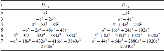
Table 1 Long description
The table presents expressions for D 0 j and B 0 j for values of j ranging from 2 to 7. Each row corresponds to a specific value of j, starting from 2 and going up to 7. The columns are labeled D 0 j and B 0 j, containing mathematical expressions involving delta (δ) raised to various powers. For example, for j equals 2, D 0 j is δ squared and B 0 j is negative δ squared. For j equals 3, D 0 j is negative δ cubed minus 26 δ squared, and B 0 j is δ cubed minus 48 δ squared. The table continues this pattern up to j equals 7, with increasingly complex expressions. The expressions involve combinations of δ raised to different powers, with coefficients that change for each value of j. The table provides a detailed mathematical breakdown of these expressions, useful for understanding the relationships and patterns in the given context.
Our goal is to find $r_0$
such that
$r_0$
such that $D_{0,r_0} \leq 0$
and
$D_{0,r_0} \leq 0$
and $B_{0,r_0} \leq 0$
(with at least one inequality being strict). Given the alternating nature of the leading terms, this is more subtle than in previous cases.
$B_{0,r_0} \leq 0$
(with at least one inequality being strict). Given the alternating nature of the leading terms, this is more subtle than in previous cases.
If r is odd, let ${\mathcal{Q}}_r$
be the statement
${\mathcal{Q}}_r$
be the statement
 \begin{align*}{\mathcal{Q}}_r\colon \quad D_{0,r} \leq -\delta^{r}-2r\delta^{r-1} \quad \text{and} \quad B_{0,r} \leq \delta^{r}-2r\delta^{r-1} .\end{align*}
If r is even, let ${\mathcal{Q}}_r$
be the statement
${\mathcal{Q}}_r$
be the statement
 \begin{align*}{\mathcal{Q}}_r\colon \quad D_{0,r}\leq -\delta^{r}-4r\delta^{r-1} \quad \text{and} \quad B_{0,r} \leq \delta^{r} .\end{align*}
We observe that ${\mathcal{Q}}_7$
holds. We now show that if
${\mathcal{Q}}_7$
holds. We now show that if ${\mathcal{Q}}_r$
holds for r odd then
${\mathcal{Q}}_r$
holds for r odd then ${\mathcal{Q}}_{r+1}$
holds, and if
${\mathcal{Q}}_{r+1}$
holds, and if ${\mathcal{Q}}_r$
holds for r even then
${\mathcal{Q}}_r$
holds for r even then ${\mathcal{Q}}_{r+1}$
holds. It will then follow by induction that
${\mathcal{Q}}_{r+1}$
holds. It will then follow by induction that ${\mathcal{Q}}_r$
holds for all
${\mathcal{Q}}_r$
holds for all $r \geq 7$
.
$r \geq 7$
.
Suppose $r \geq 3$
is odd and
$r \geq 3$
is odd and ${\mathcal{Q}}_r$
holds. Then
${\mathcal{Q}}_r$
holds. Then
 \begin{align*} D_{0,r+1} &= \delta D_{0,r}+2(1+\delta) B_{0,r}\\ &\leq \delta(\!-\delta^{r}-2r\delta^{r-1})+2(1+\delta)(\delta^{r}-2r\delta^{r-1})\\ &= \delta^{r+1}-(6r-2)\delta^{r}-4r\delta^{r-1}\\ &\leq \delta^{r+1}-4(r+1)\delta^{r}, \end{align*}
where the last inequality holds since $2r \geq 6$
. Moreover,
$2r \geq 6$
. Moreover,
 \begin{align*} B_{0,r+1}& = \delta D_{0,r}+2r B_{0,r}\\ &\leq \delta(\!-\delta^{r}-2r\delta^{r-1})+2r(\delta^{r}-2r\delta^{r-1})\\ &= -\delta^{r+1}-4r^{2}\delta^{r-1}\\ &\leq -\delta^{r+1}. \end{align*}
Hence ${\mathcal{Q}}_{r+1}$
holds. Now suppose
${\mathcal{Q}}_{r+1}$
holds. Now suppose $r \geq 2$
is even and
$r \geq 2$
is even and ${\mathcal{Q}}_r$
holds. Then
${\mathcal{Q}}_r$
holds. Then
 \begin{align*} D_{0,r+1}& = \delta D_{0,r}+2(1+\delta) B_{0,r}\\ &\leq \delta(\delta^{r}-4r\delta^{r-1})-2(1+\delta)\delta^{r}\\ &= -\delta^{r+1}-(4r+2)\delta^{r}\\ &\leq -\delta^{r+1}-2(r+1)\delta^{r} \end{align*}
and
 \begin{align*}B_{0,r+1}&= \delta D_{0,r}+2r B_{0,r}\\[3pt] &\leq \delta(\delta^{r}-4r\delta^{r-1})-2r\delta^{r}\\[3pt] &=\delta^{r+1}-6r\delta^{r}\\[3pt] &\leq\delta^{r+1}-2(r+1)\delta^{r}. \end{align*}
We conclude that ${\mathcal{Q}}_{r+1}$
holds.
${\mathcal{Q}}_{r+1}$
holds.
It follows by induction that ${\mathcal{Q}}_r$
holds for all
${\mathcal{Q}}_r$
holds for all $r \geq 7$
. Given
$r \geq 7$
. Given $\delta>0$
, choose
$\delta>0$
, choose $r^* \geq 7$
with r odd such that
$r^* \geq 7$
with r odd such that $2r^*>\delta$
. Then
$2r^*>\delta$
. Then ${\mathcal{Q}}_{r^*}$
holds. In particular,
${\mathcal{Q}}_{r^*}$
holds. In particular, $D_{0,r^*}<0$
holds and, by closer inspection of the statement of
$D_{0,r^*}<0$
holds and, by closer inspection of the statement of ${\mathcal{Q}}_r$
, also
${\mathcal{Q}}_r$
, also $B_{0,r^*}<0$
. Hence
$B_{0,r^*}<0$
. Hence $H<0$
.
$H<0$
.
Finally, we extend the result that for all $\delta>0$
there exists
$\delta>0$
there exists $r^*$
such that
$r^*$
such that $\Lambda_{D_{0,r^*},B_{0,r^*},r^*} < 0$
from the case
$\Lambda_{D_{0,r^*},B_{0,r^*},r^*} < 0$
from the case $\alpha=0$
to
$\alpha=0$
to $\alpha>0$
. Let
$\alpha>0$
. Let ${\mathcal{R}}_r$
be the statement
${\mathcal{R}}_r$
be the statement
 \begin{align*} {\mathcal{R}}_r\colon \quad D_{\alpha,r}\leq D_{0,r}\quad \text{and} \quad B_{\alpha,r}\leq B_{0,r} \end{align*}
where $D_{\alpha,r}$
and
$D_{\alpha,r}$
and $B_{\alpha,r}$
are given by the iterations in (A.7) and (A.8). Note that
$B_{\alpha,r}$
are given by the iterations in (A.7) and (A.8). Note that ${\mathcal{R}}_0$
is true since
${\mathcal{R}}_0$
is true since $ D_{\alpha,0}= D_{0,0}=1$
and
$ D_{\alpha,0}= D_{0,0}=1$
and $ B_{\alpha,0}= B_{0,0}=-1$
. Note also that
$ B_{\alpha,0}= B_{0,0}=-1$
. Note also that $D_{0,r}+B_{0,r} \leq 0$
for all
$D_{0,r}+B_{0,r} \leq 0$
for all $r \geq 0$
, by inspection for
$r \geq 0$
, by inspection for $r \leq 7$
and by the fact that
$r \leq 7$
and by the fact that ${\mathcal{Q}}_r$
is true for all
${\mathcal{Q}}_r$
is true for all $r \geq 7$
.
$r \geq 7$
.
Assume that ${\mathcal{R}}_r$
holds for
${\mathcal{R}}_r$
holds for $r=k$
. Then
$r=k$
. Then
 \begin{align*} D_{\alpha,k+1}&= D_{\alpha,k}(\alpha+\delta)+ B_{\alpha,k}(\alpha+2+2\delta)\\[5pt] &\leq D_{0,k}(\alpha+\delta)+ B_{0,k}(\alpha+2+2\delta)\\[5pt] &= \alpha( D_{0,k}+ B_{0,k})+\delta D_{0,k}+(2+2\delta) B_{0,k}\\[5pt] &= \alpha( D_{0,k}+ B_{0,k})+ D_{0,k+1}\\[5pt] &\leq D_{0,k+1}. \end{align*}
Similarly, since ${\mathcal{R}}_k$
holds,
${\mathcal{R}}_k$
holds,
 \begin{align*} B_{\alpha,k+1}&= D_{\alpha,k}(\alpha+\delta)+ B_{\alpha,k}(2k+\alpha)\\[5pt] &\leq D_{0,k}(\alpha+\delta)+ B_{0,k}(2k+\alpha)\\[5pt] &= \alpha( D_{0,k}+ B_{0,k})+\delta D_{0,k}+2k B_{0,k}\\[5pt] &= \alpha( D_{0,k}+ B_{0,k})+ B_{0,k+1}\\[5pt] &\leq B_{0,k+1}. \end{align*}
Hence ${\mathcal{R}}_{k+1}$
holds, and we conclude that
${\mathcal{R}}_{k+1}$
holds, and we conclude that ${\mathcal{R}}_r$
holds for all r. Recall that for all
${\mathcal{R}}_r$
holds for all r. Recall that for all $\delta>0$
there exists
$\delta>0$
there exists $r^*$
with
$r^*$
with $r^* \geq 7$
with
$r^* \geq 7$
with $r^*$
odd such that
$r^*$
odd such that $2 r^*> \delta$
, and then
$2 r^*> \delta$
, and then $ D_{0,r^{*}}<0$
and
$ D_{0,r^{*}}<0$
and $ B_{0,r^{*}}<0$
. Then we also have
$ B_{0,r^{*}}<0$
. Then we also have $ D_{\alpha,r^{*}}\leq D_{0,r^{*}}<0$
and
$ D_{\alpha,r^{*}}\leq D_{0,r^{*}}<0$
and $ B_{\alpha,r^{*}}\leq B_{0,r^{*}}<0$
. Hence
$ B_{\alpha,r^{*}}\leq B_{0,r^{*}}<0$
. Hence $H= \Lambda_{D_{\alpha,r^*},B_{\alpha,r^*},r^*}<0$
as required.
$H= \Lambda_{D_{\alpha,r^*},B_{\alpha,r^*},r^*}<0$
as required.
Acknowledgement
We wish to thank Jon Warren for useful conversations about the Bessel process.
Funding information
There are no funding bodies to thank relating to the creation of this article.
Competing interests
There were no competing interests to declare which arose during the preparation or publication process of this article.

 X(ω)=(Xt(ω))0≤t≤1
 c(s)=C1−s
 C≈1.50339538
 τ∗(ω)=inf{u∈(0,1):Xu(ω)≥C(1−u)}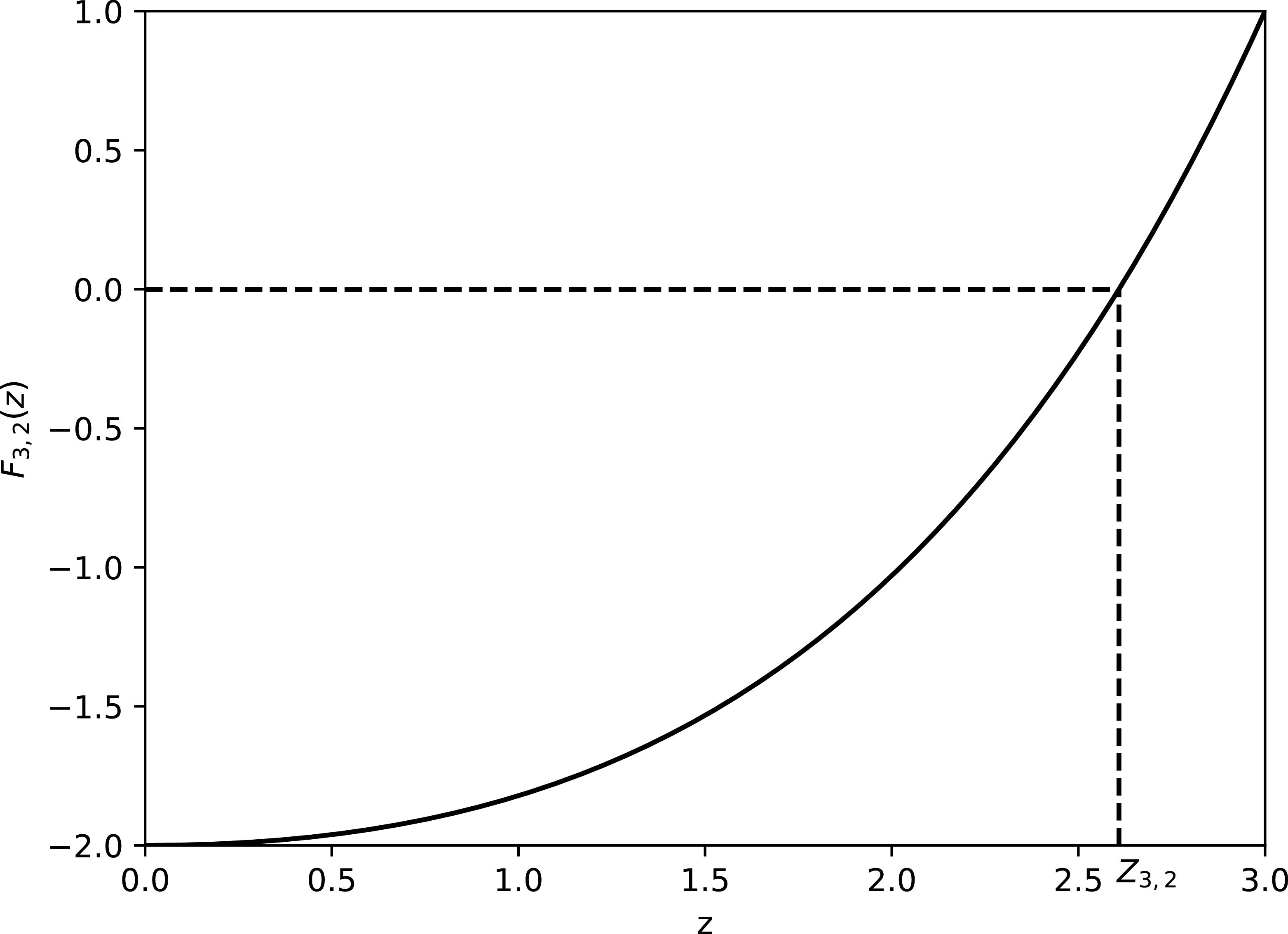
 Fα,n(z)
 α=3
α=3 n=2
n=2 Z3,2
Z3,2 Z3,2>(3+2−2)/2=1.5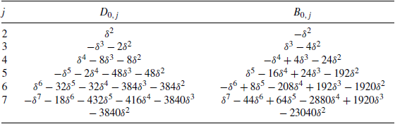
 D0,j
D0,j B0,j
B0,j 2≤j≤7
2≤j≤7
 Open access

