

Non-technical Summary
The early Maastrichtian (ca. 70 Ma) ammonoid genus Gunnarites in the James Ross Basin (JRB) of Antarctica occurs in a relatively narrow stratigraphic interval, spanning a geologically short time, which also marks a period of cooling temperatures and a local drop in sea level. The presence of Gunnarites is an important tool for identifying this interval at different locations across the JRB. Early studies of Gunnarites qualitatively described differences in shape among specimens from different locations in the JRB, in some cases attributing these shape differences to different species of Gunnarites. If real, these morphological differences among locations could affect how Gunnarites is used for biostratigraphy in the JRB and could improve our understanding of the factors that control ammonite shell shape.
We measured a variety of morphological traits for 118 Gunnarites specimens from seven locations in the JRB to test whether shape varies by location. We used statistical models to quantify differences in ammonite shell shape and ornamentation between locations, while also accounting for variation in specimen size. Most morphological traits showed significant differences between locations, but the patterns of variation across the JRB differed. The location-based morphological differences for Gunnarites might be the result of several factors: (1) shape variation driven by environmental differences among analyzed locations across the JRB; (2) change(s) in shape over time (e.g., evolution) with different localities representing different time periods; (3) stratigraphic repetition from previously hypothesized faults or folds; or (4) a combination of these factors. More precise, independent, age-dating of each location is needed to distinguish the possible causes of the morphological variation revealed in this study.
Introduction
The James Ross Basin (JRB), Antarctica, contains one of the most complete Upper Cretaceous sedimentary marine records in the southern high paleolatitudes (e.g., Zinsmeister, Reference Zinsmeister1982; Macellari, Reference Macellari1988a; Pirrie et al., Reference Pirrie, Crame, Lomas and Riding1997; McArthur et al., Reference McArthur, Crame and Thirlwall2000; Crame et al., Reference Crame, Francis, Cantrill and Pirrie2004; Olivero, Reference Olivero2012a; Milanese et al., Reference Milanese, Olivero, Raffi, Franceschinis, Gallo, Skinner, Mitchell, Kirschvink and Rapalini2019b; Roberts et al., Reference Roberts, O’Connor, Clarke, Slotznick and Placzek2023; Crame and Francis, Reference Crame and Francis2024) and has been the subject of many studies seeking to characterize the sedimentology, biostratigraphy, and environmental conditions of the Late Cretaceous (e.g., Barreda et al., Reference Barreda, Palazzesi and Olivero2019; Crame, Reference Crame2019; Lamanna et al., Reference Lamanna, Case, Roberts, Arbour, Ely, Salisbury, Clarke, Malinzak, West and O’Connor2019; Montes et al., Reference Montes, Beamud, Nozal and Santillana2019; Raffi et al., Reference Raffi, Olivero and Milanese2019; Mohr et al., Reference Mohr, Tobin, Petersen, Dutton and Oliphant2020; Scasso et al., Reference Scasso, Prámparo, Vellekoop, Franzosi, Castro and Sinninghe Damsté2020; Piovesan et al., Reference Piovesan, Correia Filho, Melo, Lacerda, Dos Santos, Pinheiro, Costa, Sayão and Kellner2021; Reguero et al., Reference Reguero, Gasparini, Olivero, Coria and Fernández2022; Videira-Santos et al., Reference Videira-Santos, Tobin and Scheffler2022; Witts and Little, Reference Witts, Little, Kaim, Cochran and Landman2022; da Silva et al., Reference da Silva, Santos, Fauth, Manríquez, Kochhann, do Monte Guerra, Horodyski, Villegas-Martín and da Silva2023; Guerrero-Murcia et al., Reference Guerrero-Murcia, Helenes, di Pasquo and Martin2023; Santiago et al., Reference Santiago, de Araújo Carvalho, Ramos and Scheffler2024). The highly fossiliferous JRB also provides a critical record of the Kossmaticeratidae, a characteristic ammonite of the Late Cretaceous invertebrate macrofauna of the southern hemisphere commonly used for biostratigraphic zonation (e.g., Kilian and Reboul, Reference Kilian and Reboul1909; Marshall, Reference Marshall1926; Spath, Reference Spath1953; Matsumoto, Reference Matsumoto1955; Howarth, Reference Howarth1958, Reference Howarth1966; Henderson, Reference Henderson1970; Lahsen and Charrier, Reference Lahsen and Charrier1972; Thomson, Reference Thomson1982; Riccardi, Reference Riccardi1983, Reference Riccardi1984; Olivero, Reference Olivero1984, Reference Olivero and Rinaldi1992, Reference Olivero2012a, Reference Oliverob; Macellari, Reference Macellari1985, Reference Macellari1986, Reference Macellari1987, Reference Macellari1988b; Crame et al., Reference Crame, Pirrie, Riding and Thomson1991; Olivero and Medina, Reference Olivero and Medina2000; Witts et al., Reference Witts, Bowman, Wignall, Crame, Francis and Newton2015). Patterns of kossmaticeratid diversity and biogeographic distribution may be linked to oceanic and climate conditions during the Late Cretaceous (Macellari, Reference Macellari1987; Olivero and Medina, Reference Olivero and Medina2000; Witts et al., Reference Witts, Bowman, Wignall, Crame, Francis and Newton2015), but morphological variation within the kossmaticeratids remains poorly characterized, limiting our understanding of this group and its biostratigraphic applications.
In the JRB, Gunnarites has been a useful tool for biostratigraphy and correlation. Its presence in one of the first collections of Antarctic fossils provided the first age estimate for the Cretaceous strata in the JRB (Weller, Reference Weller1903), although the collector, F. W. Stokes, was later accused of scientific misconduct regarding the publication of these specimens (breaking an agreement to withhold scientific results of the Swedish Antarctic Expedition until the conclusion of their second field season, and misattributing the specimens to the Belgian Antarctic Expedition; see Andersson, Reference Andersson1906, p. 34). More recently, Gunnarites has been recognized as a macrofossil marker for the base of the Maastrichtian (Crame et al., Reference Crame, McArthur, Pirrie and Riding1999), although magnetostratigraphic evidence now places the first appearance datum for Gunnarites within the lower Maastrichtian (Milanese et al., Reference Milanese, Olivero, Slotznick, Tobin, Raffi, Skinner, Kirschvink and Rapalini2020). Gunnarites is a particularly important taxon for understanding the JRB because it has a relatively short temporal range (1–2 Myr; see “Geologic Setting”) and its presence defines a biostratigraphic interval that is geographically distributed across many isolated localities within the JRB. This interval coincides with an increase in the endemism of ammonite fauna in the JRB (Macellari, Reference Macellari1987; Olivero and Medina, Reference Olivero and Medina2000; Witts et al., Reference Witts, Bowman, Wignall, Crame, Francis and Newton2015) and other abiotic changes that occur across the Campanian–Maastrichtian boundary, including global cooling (Ditchfield et al., Reference Ditchfield, Marshall and Pirrie1994; Huber et al., Reference Huber, Hodell and Hamilton1995; Barrera and Savin, Reference Barrera and Savin1999) and local regression (Olivero and Medina, Reference Olivero and Medina2000; Olivero, Reference Olivero2012a).
For biostratigraphic purposes in the JRB, Gunnarites (sensu lato) has been treated as a homogeneous group, and species-level identifications of specimens are not required to recognize ammonite zones defined by Gunnarites. However, previous taxonomic work suggests that Gunnarites conch and ornament morphology varies across locations within the JRB. Spath (Reference Spath1953) proposed 18 distinct species and varieties of Gunnarites in the JRB, 11 of which were taxa unique to a single location: G. flexuosus and G. pachys and their subspecific varieties were unique to Humps Island, G. rotundus and G. paucinodatus and their varieties were unique to Lachman Crags South, G. gunnari (Kilian and Reboul, Reference Kilian and Reboul1909) was unique to The Naze, G. antarcticus var. monilis was unique to Spath Peninsula, and G. bhavaniformis var. vegaensis was unique to False Island Point (see “Geologic Setting” and Fig. 1). Even after significant taxonomic revision and synonymization of the genus, Howarth (Reference Howarth1966) still retained a species unique to Humps Island (G. pachys), suggesting a distinct Gunnarites morphology occurring at that location (but see Olivero, Reference Olivero and Rinaldi1992, for a critique of Howarth’s synonymization). Supplementary Table 8 provides a summary of the morphological characters used by Spath (Reference Spath1953) and Howarth (Reference Howarth1966) to distinguish among species and varieties of Gunnarites in the JRB.
Locations (stars) where Gunnarites occur in the James Ross Basin, with inset showing location of James Ross Basin on the Antarctic Peninsula, after Crame et al. (Reference Crame, Francis, Cantrill and Pirrie2004) and Tobin et al. (Reference Tobin, Flannery and Sousa2018). Colored stars show Gunnarites locations included in this study, each labeled with sample size (number of specimens) and location abbreviations used in subsequent figures: Santa Marta Cove (SMC), The Naze (NZ), False Island Point (FIP), Ula Point (ULA), Day Nunatak (DAY), and Sanctuary Cliffs (SC).

If significant morphological differences between locations do exist for JRB Gunnarites, those patterns could have important implications for their use for inter-basin correlations, or for our understanding of Gunnarites ecology and evolution over this environmentally dynamic interval. Many factors may contribute to morphological variation in ammonites, including differences within individuals (e.g., ontogeny), among individuals (e.g., sexes, species), and variation across space (e.g., environmental gradients) or time (e.g., evolution; De Baets et al., Reference De Baets, Bert, Hoffmann, Monnet, Yacobucci, Klug, Klug, Korn, De Baets, Kruta and Mapes2015; Monnet et al., Reference Monnet, De Baets, Yacobucci, Klug, Korn, De Baets, Kruta and Mapes2015). Quantifying patterns in ammonite size and shape can help distinguish among these different possible sources of morphological variation (e.g., De Baets et al., Reference De Baets, Jarochowska, Buchwald, Klug and Korn2022; Mohr et al., Reference Mohr, Tobin and Tompkins2024), improving our understanding of ammonite taxonomy, evolution, and ecology.
Previously hypothesized (qualitatively described but not quantitatively evaluated) location-based morphological differences for JRB Gunnarites (e.g., Spath, Reference Spath1953; Howarth, Reference Howarth1966) highlight the utility of this group as a case study to explore spatial and temporal influences on ammonite morphology. To evaluate the possible factors influencing Gunnarites morphology, we must first test whether the previously reported morphological variation is real, and, if so, document its nature and magnitude. In this study, we use linear mixed models (LMMs) and generalized additive mixed models (GAMMs) to quantitatively evaluate whether Gunnarites exhibits morphological differences across locations within the JRB. Using mixed models enables us to accommodate for the nested data structure of mixed longitudinal sampling (with measurements of multiple ontogenetic stages for each specimen) and account for within-individual morphological variation. We explore possible explanations for morphological patterns in our data and highlight future directions for research in the Gunnarites interval of the JRB.
Geologic setting
The James Ross Basin (JRB) is a back-arc basin located at the NE tip of the Antarctic Peninsula and contains a fossiliferous and expanded marine sedimentary section of the Upper Cretaceous (Crame and Francis, Reference Crame and Francis2024, and references therein). The Marambio Group is a >3000-m-thick section recording a prograding shelf environment from the Santonian through the Danian, which is subdivided into three stratigraphic sequences (Olivero and Medina, Reference Olivero and Medina2000) and 15 ammonite assemblages (Olivero, Reference Olivero2012a, Reference Oliverob). In the JRB, Gunnarites occurs within “Ammonite Assemblage 9” (AA9) and “Ammonite Assemblage 10” (AA10) of the second sequence, the NG Sequence (named for Neograhamites and Gunnarites; Olivero and Medina, Reference Olivero and Medina2000); AA9 is characterized by the first appearance of Gunnarites and the co-occurrence of Neograhamites cf. N. kiliani Spath, Reference Spath1953, and AA10 is characterized by an ammonite fauna dominated by Gunnarites (Olivero, Reference Olivero2012a).
The duration of the Gunnarites assemblage in the JRB (AA9 and AA10) is thought to be relatively short (<1 Myr), but this interval is only constrained within a single magnetochron (C31r, ca. 2.2 Myr; Milanese et al., Reference Milanese, Olivero, Raffi, Franceschinis, Gallo, Skinner, Mitchell, Kirschvink and Rapalini2019b). Gunnarites fossils are found throughout approximately half of the stratigraphic interval where C31r is measured, and with simple interpolation, this genus range would correspond to approximately 1 Myr. However, without additional geochronological evidence, this time interval could be much shorter or longer (Husson et al., Reference Husson, Galbrun, Laskar, Hinnov, Thibault, Gardin and Locklair2011; Ogg, Reference Ogg, Gradstein, Ogg, Schmitz and Ogg2020). The entire Gunnarites assemblage in the JRB occurs within the early Maastrichtian and the base of the Gunnarites assemblage has often been placed as synchronous, or nearly so, with the Campanian–Maastrichtian boundary, as supported by strontium isotope correlation (Crame et al., Reference Crame, McArthur, Pirrie and Riding1999, Reference Crame, Francis, Cantrill and Pirrie2004; Roberts et al., Reference Roberts, O’Connor, Clarke, Slotznick and Placzek2023). However, recent magnetostratigraphic work places the first occurrence of Gunnarites within the early Maastrichtian (Milanese et al., Reference Milanese, Olivero, Raffi, Franceschinis, Gallo, Skinner, Mitchell, Kirschvink and Rapalini2019b, Reference Milanese, Olivero, Slotznick, Tobin, Raffi, Skinner, Kirschvink and Rapalini2020), although the precise timing is uncertain. The top of the Gunnarites assemblage is thought to be diachronous across the basin (Crame et al., Reference Crame, Francis, Cantrill and Pirrie2004), although this may be in large part controlled by differential erosion and/or non-deposition.
Regardless of the precise age and duration of the Gunnarites range zone, it remains an important biostratigraphic zone to understand the JRB. In contrast to the Santonian–Campanian and Maastrichtian–Danian intervals, which are represented by mostly continuous stratigraphic exposures on James Ross Island (Olivero et al., Reference Olivero, Scasso and Rinaldi1986; Crame et al., Reference Crame, Pirrie, Riding and Thomson1991) or Seymour Island (Zinsmeister et al., Reference Zinsmeister, Feldmann, Woodburne and Elliot1989; Elliot et al., Reference Elliot, Askin, Kyte and Zinsmeister1994; Tobin et al., Reference Tobin, Ward, Steig, Olivero, Hilburn, Mitchell, Diamond, Raub and Kirschvink2012), respectively, the uppermost Campanian–lowermost Maastrichtian interval is exposed only in geographically small and stratigraphically thin successions spread across the basin (Pirrie et al., Reference Pirrie, Crame, Lomas and Riding1997; Crame et al., Reference Crame, Francis, Cantrill and Pirrie2004; Olivero, Reference Olivero2012a; Tobin et al., Reference Tobin, Flannery and Sousa2018).
Figure 1 shows all the localities in the JRB from which Gunnarites has been reported. These sites form a roughly NW–SE transect across the basin that generally corresponds to a gradient from nearshore (NW) to offshore (SE) deposition at any given time (Olivero, Reference Olivero2012a, and references therein). However, the shoreline also prograded to the SE during the Gunnarites interval such that any given succession could include deposition representing a range of paleodepths. Additionally, the strata of the JRB have a general regional dip of 10° to the SE, largely due to differential subsidence of the basin during and after deposition (Bibby, Reference Bibby1966; Crame et al., Reference Crame, Pirrie, Riding and Thomson1991). The paleolatitude of the JRB (62°S; Tobin et al., Reference Tobin, Ward, Steig, Olivero, Hilburn, Mitchell, Diamond, Raub and Kirschvink2012; Milanese et al., Reference Milanese, Rapalini, Slotznick, Tobin, Kirschvink and Olivero2019a) is approximately the same as today.
Some structural complexity exists within the JRB, which may complicate the simple NW–SE deepening trend. Different bedding attitudes have been observed at some localities, particularly on Vega Island and northern James Ross Island (shallow dip to the NE instead of SE). Additionally, minor (<10 m of bedding offset) faulting (both normal and reversed) is visible at localities including Humps Island, and from exposures in the SE part of James Ross Island. These features themselves are insufficient to change basin-scale patterns, but they have been used to propose larger scale folding or faulting along a roughly NE–SW axis (Bibby, Reference Bibby1966; Medina et al., Reference Medina, Scasso, del Valle, Olivero, Malagnino, Rinaldi, Chebli and Spalletti1989; Crame et al., Reference Crame, Pirrie, Riding and Thomson1991; Strelin et al., Reference Strelin, Scasso, Olivero and Rinaldi1992; Crame and Luther, Reference Crame and Luther1997; Crame and Francis, Reference Crame and Francis2024). However, the limited exposure outside of these localities (due to permanent ice cover and much younger basaltic cap rocks) has made recognition of map-scale structural features difficult.
Gunnarites is primarily restricted to the Snow Hill Island Formation (SHIF), although the youngest occurrence is recorded from the overlying Haslum Crag Sandstone on the eastern edge of the basin (Pirrie et al., Reference Pirrie, Crame, Lomas and Riding1997; Olivero et al., Reference Olivero, Ponce and Martinioni2008). Per Olivero (Reference Olivero2012a, and references therein), the SHIF is subdivided into several members, including the Gamma and Cape Lamb members on the western side of the basin, and the Hamilton Point, Sanctuary Cliffs, and Karlsen Cliffs members on the eastern side of the basin. However, other subdivisions have also been employed (see Roberts et al., Reference Roberts, O’Connor, Clarke, Slotznick and Placzek2023, and Crame and Francis, Reference Crame and Francis2024, for a comparison of these approaches). Here, we make use of Olivero’s (Reference Olivero2012a) approach, but the current study does not argue for or against any particular stratigraphic nomenclature.
In the western half of the basin, Gunnarites is found within the upper third of the Gamma Member of the SHIF, which is largely comprised of shelf mudstones and sandstones deposited above storm wave base but below fair-weather wave base, representing a deeper depositional facies than the lower part of the unit (Pirrie, Reference Pirrie1990; Scasso et al., Reference Scasso, Olivero and Buatois1991). Gunnarites are also found throughout much of the Cape Lamb Member, which represents more offshore deposition with finer sediments than the Gamma Member. Gunnarites are not known from the uppermost Cape Lamb Member (below the basal conglomerate of the López de Bertodano Formation in the stratigraphic approach of Olivero, Reference Olivero2012a), which represents more proximal, sandier, deposition. The eastern half of the basin is typically interpreted as more distal sedimentation, with the Sanctuary Cliffs Member including offshore mudstones and rare distal, storm-derived sandstones, shallowing upsection into the Karlsen Cliffs Member, which is unconformably overlain by the Haslum Crag Sandstone. Gunnarites are abundant from the upper 20–30 m of the Sanctuary Cliffs Member and throughout the Karlsen Cliffs Member, and additional specimens (often poorly preserved) are occasionally found in the Haslum Crag Sandstone, which crops out on Snow Hill and Seymour Islands and represents much more proximal deposition. This sequence represents the thickest total stratigraphic interval from which Gunnarites is known, encompassing approximately 350 m of stratigraphic section.
Locations
In this study we analyzed specimens from seven of the locations from which Gunnarites is known in the JRB. Below we briefly summarize relevant details (see also Fig. 2) from the existing literature and refer the reader to the more comprehensive studies of Olivero (Reference Olivero2012a) and Crame and Francis (Reference Crame and Francis2024) for a more detailed account of the sedimentology and stratigraphy of these areas.
Simplified sequence stratigraphic diagram of Upper Cretaceous outcrops in the James Ross Basin, Antarctica, after Olivero (Reference Olivero2012a). Ammonite Assemblages 9 and 10 (AA9 and AA10) of Olivero (Reference Olivero2012a) shown in shaded blue area and labeled “Gunnarites Zone.” Abbreviations of studied Gunnarites locations as in Figure 1. Gray fill color indicates that Gunnarites does not occur in a given section; hollow or color fill indicates that Gunnarites does occur. Studied Gunnarites sections are filled with a unique color per locality that corresponds to locality colors in Figures 1, 6–9. See “Geological Setting” in text for justification of placement of studied locations in either AA9 or AA10.

Most of the studied Gunnarites specimens were collected opportunistically during brief (one day or less) field excursions, and/or were collected as float without precise horizon information. All seven localities had relatively thin stratigraphic exposures, generally less than 50 m, from which Gunnarites were collected. Estimated sediment accumulation rates for the JRB range between ~10–50 cm/kyr and may vary spatially depending on facies (Milanese et al., Reference Milanese, Olivero, Raffi, Franceschinis, Gallo, Skinner, Mitchell, Kirschvink and Rapalini2019b, Reference Milanese, Olivero, Slotznick, Tobin, Raffi, Skinner, Kirschvink and Rapalini2020), such that each studied locality may represent <0.1–0.5 Myr of deposition. Because we cannot attribute most specimens to a specific stratum, and there are variations in sedimentology within most studied successions, specimens from a given location may have originated from a range of depositional environments, and, to some extent, paleodepths. Our studied localities cannot be individually categorized as either entirely nearshore or entirely offshore, but are better characterized as part of a gradient, such that successions at NW or SE localities tend to have more nearshore or more offshore deposition, respectively.
Santa Marta Cove, James Ross Island (SMC)
Santa Marta Cove is located on the northern Ulu Peninsula of James Ross Island. At this locality, Gunnarites are typically reported only from the vicinity of Santa Marta Cove (e.g., Olivero et al., Reference Olivero, Scasso and Rinaldi1986; Crame et al., Reference Crame, Francis, Cantrill and Pirrie2004). Spath (Reference Spath1953) also described Gunnarites specimens from east-dipping beds in “Lachman Crags, South,” a location on the eastern edge of Ulu Peninsula, north of Santa Marta Cove, but these specimens have since been reclassified as Natalites belonging to earlier ammonite assemblages (AA5 and AA6; Olivero, Reference Olivero and Rinaldi1992; Olivero and Medina, Reference Olivero and Medina2000) and were not included in our study (see “Materials”). Our specimens are derived from gently north-dipping beds at localities QF and 14S of Santa Marta Cove (Olivero, Reference Olivero and Rinaldi1992; Strelin et al., Reference Strelin, Scasso, Olivero and Rinaldi1992; Milanese et al., Reference Milanese, Olivero, Slotznick, Tobin, Raffi, Skinner, Kirschvink and Rapalini2020), which are located in the upper portion of the Gamma Member of the SHIF. The section here (see Olivero, Reference Olivero2012b, fig. 2) includes (from bottom to top) the localities Hy, Hy20, and QF-14S (see map in Olivero, Reference Olivero and Rinaldi1992, fig. 1). While QF-14S beds only contain the AA9, the stratigraphically lower localities Hy20 and Hy contain the AA8-2 (an assemblage characterized by the abundance of Neograhamites cf. N. kiliani and absence of Gunnarites). These intervals represent less than 50 m of exposed stratigraphy.
The Naze, James Ross Island (NZ)
The Naze is a peninsula protruding to the NE from James Ross Island and includes a stratigraphically thin (<50 m) exposure of the Cape Lamb Member of the Snow Hill Island Formation (SHIF) (del Valle et al., Reference del Valle, Fourcade, Medina and Craddock1982; Piovesan et al., Reference Piovesan, Correia Filho, Melo, Lacerda, Dos Santos, Pinheiro, Costa, Sayão and Kellner2021). Gunnarites are found throughout the outcrop, which is largely comprised of subhorizontal, poorly indurated mudstones. This outcrop roughly corresponds to the published sections A and B of Piovesan et al. (Reference Piovesan, Correia Filho, Melo, Lacerda, Dos Santos, Pinheiro, Costa, Sayão and Kellner2021, fig. 2) and the section of del Valle et al. (Reference del Valle, Fourcade, Medina and Craddock1982, fig. 30.2). This interval has been interpreted to represent AA10 (di Pasquo and Martin, Reference di Pasquo and Martin2013).
False Island Point, Vega Island (FIP)
False Island Point is a peninsula protruding south from Vega Island. Similar to The Naze, a thin exposure (less than 50 m of stratigraphy was sampled) of the Cape Lamb Member of the SHIF is present, which is comprised of poorly indurated mudstones, but this exposure may be somewhat up-section and therefore younger than strata from The Naze (based on bedding orientations and locality positions) and represents AA10 (Olivero, Reference Olivero2012a, Fig. 2).
Humps Island (HI)
Humps Island is a small island a short distance south from False Island Point and The Naze, but the exposure here differs significantly from those locations in several ways, despite also being interpreted as primarily an exposure of the Cape Lamb Member. The lower ~50 m of strata on Humps Island, from which all of the Gunnarites were collected, are mixed sandy siltstones and poorly indurated mudstones, with common calcareous resistant horizons, gently dipping to the west. This lower unit has been attributed to the Gamma Member of the SHIF (or its proximal equivalent Herbert Sound Member; Dolding, Reference Dolding1992). This interval is overlain by ~40 m of largely barren mudstone, capped by younger James Ross Island volcanic rocks. The precise stratigraphic relationship of Humps Island to nearby exposures has been the subject of debate (e.g., Spath, Reference Spath1953; Bibby, Reference Bibby1966; Howarth, Reference Howarth1966; Pirrie and Riding, Reference Pirrie and Riding1988; Dolding, Reference Dolding1992). Olivero (Reference Olivero2012a) placed Humps Island within AA9 based on the co-occurrence of Neograhamites with Gunnarites. However, most fossils from Humps Island are recovered somewhat out of context after tumbling down relatively steep slopes, so it cannot be determined if AA10 (Gunnarites absent Neograhamites) is also present here. The sampled section corresponds to the published section of Pirrie and Riding (Reference Pirrie and Riding1988, fig. 2a) and sections D.8673 and HI of Wood and Askin (Reference Wood and Askin1992, figs. 1–3).
Ula Point, James Ross Island (ULA)
Ula Point (unrelated to Ulu Peninsula) has received less study than most of the other sites (Bibby, Reference Bibby1966; Stilwell and Zinsmeister, Reference Stilwell and Zinsmeister1987), but largely consists of mixed clastic lithologies, which are generally poorly indurated except in concretionary horizons. This interval is considered part of the Karlsen Cliffs Member of the SHIF and is placed in AA10 due to the lack of Neograhamites (Stilwell and Zinsmeister, Reference Stilwell and Zinsmeister1987; Olivero, Reference Olivero2012a, fig. 2). The sampled specimens from Ula Point come from less than 50 m of exposed stratigraphy.
Day Nunatak, Snow Hill Island (DAY)
Day Nunatak was recently described as a part of the Karlsen Cliffs Member of the SHIF and is placed in AA10 due to the lack of Neograhamites (Tobin et al., Reference Tobin, Flannery and Sousa2018). Over 170 m of stratigraphy is exposed here and rare Gunnarites specimens are found throughout the succession (Tobin et al., Reference Tobin, Flannery and Sousa2018, fig. 5), but almost all specimens were recovered from a fossiliferous interval in the top 20 m of the section, including all but two of the specimens analyzed here. Those two specimens were found about 90 m lower, but in unconstrained float, and likely originated somewhat higher in the stratigraphic section, possibly as high as the other specimens.
Sanctuary Cliffs, Snow Hill Island (SC)
Sanctuary Cliffs is a larger nunatak (an isolated ridge protruding from surrounding ice cover) than Day Nunatak and has received comparably more (albeit still limited) geologic study (e.g., Concheyro et al., Reference Concheyro, Robles Hurtado and Olivero1994; Olivero and Aguirre-Urreta, Reference Olivero and Aguirre-Urreta1994; Robles Hurtado and Concheyro, Reference Robles Hurtado and Concheyro1995; Pirrie et al., Reference Pirrie, Crame, Lomas and Riding1997; Milanese et al., Reference Milanese, Olivero, Raffi, Franceschinis, Gallo, Skinner, Mitchell, Kirschvink and Rapalini2019b, Reference Milanese, Olivero, Slotznick, Tobin, Raffi, Skinner, Kirschvink and Rapalini2020). It exposes the Sanctuary Cliffs Member of the SHIF, the upper levels (~30 m) of which are placed in AA9 based on the presence of Gunnarites (Olivero and Medina, Reference Olivero and Medina2000; Olivero, Reference Olivero2012a; Raffi et al., Reference Raffi, Olivero and Milanese2019). The stratigraphic section at Sanctuary Cliffs is illustrated in Pirrie et al. (Reference Pirrie, Crame, Lomas and Riding1997, fig. 8, as DJ.740) and in Milanese et al. (Reference Milanese, Olivero, Raffi, Franceschinis, Gallo, Skinner, Mitchell, Kirschvink and Rapalini2019b, fig. 8).
Materials and methods
Materials
We studied 118 Gunnarites specimens from the James Ross Basin, Antarctica, including 90 specimens collected from the field (53 reposited at ALMNH, 37 reposited at CADIC/MACN) and 28 specimens figured in the existing literature (Spath, Reference Spath1953). Our dataset includes every figured Antarctic Gunnarites specimen in Spath (Reference Spath1953), with a few exceptions. We excluded two individuals from locations not otherwise represented by our data (C.41335, from Cockburn Island; C.41359, from Spath Peninsula on Snow Hill Island) and one fragment (C.41399). We also excluded specimen C.41384 for which only the innermost whorls (~5 mm diameter) were figured, because of the lack of diagnostic characteristics permitting a positive identification of genus. We also excluded any specimens from the Lachman Crags South locality on James Ross Island because this site has been interpreted as older (AA5 and AA6) than the Gunnarites assemblage (AA9 and AA10) and these specimens were reclassified as Natalites due to the lack of diagnostic crenulations on the ribs (Olivero, Reference Olivero and Rinaldi1992; Olivero and Medina, Reference Olivero and Medina2000). Even Spath (Reference Spath1953) doubted whether his Lachman Crags specimens could be referred to Gunnarites, because they lacked crenulations.
Our Gunnarites specimens are from seven different locations within the JRB (see Fig. 1 and “Geologic Setting”): 6 from Santa Marta Cove (James Ross Island), 43 from The Naze (James Ross Island), 24 from Ula Point (James Ross Island), 9 from False Island Point (Vega Island), 10 from Humps Island, 8 from Sanctuary Cliffs (Snow Hill Island), and 18 from Day Nunatak (Snow Hill Island).
The typical usage of Gunnarites for zonation and correlation within the JRB requires only a genus-level identification, which is based on the recognition of characteristic features including finely crenulated ribs (Kilian and Reboul, Reference Kilian and Reboul1909; Spath, Reference Spath1953; Olivero, Reference Olivero and Rinaldi1992). Mature modifications for Gunnarites are poorly understood (Spath, Reference Spath1953; Kennedy and Klinger, Reference Kennedy and Klinger1985), and adult specimens are not required for genus identification or for biostratigraphy. In some cases, the body chamber of large and/or mature individuals shows a marked reduction (either real or taphonomic) in the prominence of features considered diagnostic for the genus (ribbing and crenulation; Spath, Reference Spath1953), suggesting that mature individuals may even be less useful for biostratigraphy than sub-mature individuals. By including a range of specimen sizes (and not just definitively mature specimens), we maximized our sample size and ensured our data represent the range of Gunnarites specimens typically used for biostratigraphy in the JRB (i.e., a range of sizes and presumably ontogenetic stages). Care was taken to separate the effects of location from those of size (ontogenetic stage) on morphology (see “Scaling Relationships for Naze Specimens”).
Data collection
All specimens not already figured in the literature were photographed from both lateral and ventral views. We then used ImageJ to collect morphometric measurements for all specimens. Following the general approach of Mohr et al. (Reference Mohr, Tobin and Tompkins2024), we used a mixed longitudinal sampling strategy and collected repeated measurements on each specimen at 45° increments of the whorl, wherever preservation permitted (a higher sampling resolution than the 90° increments used by Mohr et al., Reference Mohr, Tobin and Tompkins2024). Exposed inner whorls on partly broken specimens were also measured opportunistically at 45° intervals. All variables were measured at each 45° increment, except for whorl width, which was only measured at 90° intervals. Whorl width measurements were duplicated with digital calipers for specimens that were physically accessible. We measured 739 unique conch positions, with an average of 6.3 measured positions per specimen (standard deviation: 1.6).
We measured standard ammonite conch morphology variables: whorl height (WH), whorl width (WW), radius (R), diameter (D), and umbilical width (U), and calculated the following dimensionless conch variables (see Fig. 3): WWI (whorl width index, or whorl shape), UWI (umbilical width index), RUWI (radial umbilical width index), WHER (whorl height expansion rate), and WRER (whorl radius expansion rate).
Morphological variables measured on Gunnarites specimens. Measured conch variables include whorl height (WH), whorl width (WW), umbilical width (U), radius (R), diameter (D). Calculated conch variables include whorl shape (WWI), umbilical width index (UWI), radial umbilical width index (RUWI), whorl height expansion rate (WHER), and whorl radius expansion rate (WRER). For expansion rate variables (WHER and WRER), WH180 and R180 are measurements of WH or R 180° prior to (earlier in ontogeny) the position of WH or R, respectively. Rib shape variables include rib angle (Z) and rib sinuosity (Ribsin). See “Data Collection” in the text for further details. Z and Ribsin are shown on different ribs for clarity: in practice, both were measured for the same rib (at each measured WH location).

We also measured or counted the following variables describing specimen ribbing. Ribsin (rib sinuosity), which is the curved length of the rib (Y) on the lateral flank, divided by the straight distance (X) between both ends of the rib. Ribsin is measured for a single rib nearest each measured 45° position on a specimen. Z (rib angle), which is an angle, in units of degrees, between both endpoints of the rib, with the vertex placed at the estimated position of the protoconch for a specimen. Z is reported as a positive value when the rib is prosiradiate, and as a negative value when the rib is rursiradiate. Z is measured for the same rib for which Ribsin was calculated. OR (outer ribs), which is a count of the number of ribs at the ventral margin of the specimen, in the previous (adapical) 45° section of whorl. IR (inner ribs) is a count of the number of ribs near the umbilical margin of the specimen (at a position just ventral of the umbilical tubercles, typically at the inner one-fourth of the flank, in the previous (adapical) 45° section of whorl.
We did not count or measure umbilical tubercles, because these features were often broken or worn. We did not count constrictions because they occur less frequently on Gunnarites specimens than our sampling resolution of 45° increments of whorl, making their presence or absence at any given ontogenetic stage somewhat random and sensitive to the starting measurement position. Measurement of constriction morphology may be useful in a future study.
Mixed model analyses
Mixed models were used at all analysis stages. These models are powerful tools for evaluating mixed longitudinal datasets because they can incorporate “random effects” associated with individual (specimen) identity, controlling for the non-independence of repeated measurements (Pinheiro and Bates, Reference Pinheiro and Bates2000). We used linear mixed models (LMMs) to detect and quantify differences in Gunnarites morphology between our studied localities while simultaneously accounting for the scaling relationships between morphological variables and increasing specimen size.
Data from our repeated measurements (i.e., measurements of multiple ontogenetic stages per specimen) display wide variation in size, both among individuals and within individuals, and non-isometric relationships between size and conch shape could obscure or artificially enhance location differences in morphology if not taken into account. We first quantified scaling relationships between size and shape using data from a single location (see “Scaling Relationships for Naze Specimens”), then included the best-supported size–shape relationships in models (fit to data from all locations) evaluating the effects of location on each morphological response variable (see “Location Effects on Morphology”). Lastly, we allowed location and size to interact, evaluating the idea that morphological differences across locations may be present only for certain size classes (see “Interactive Effects of Size and Location”).
We evaluated location differences in morphology for nine response variables: WWI, UWI, RUWI, WHER, WRER, Z, Ribsin, OR, and IR. The conch morphology variables were log-transformed before being included in the LMMs to increase the normality of their distributions; variables related to ornamentation (Z, Ribsin, OR, and IR) were not transformed. All models, for all analyses, included specimen identity (i.e., a unique identifier per specimen) as a random intercept, accounting for mean differences in the response variable between specimens. Explanatory variables (“fixed effects”) included log-transformed WH (our proxy for size), and a multi-level factor variable identifying the location for each specimen.
Count variables often follow a Poisson distribution (Zuur et al., Reference Zuur, Ieno, Walker, Saveliev and Smith2009), and rib counts (IR and OR) were initially modeled with Poisson generalized linear mixed models (GLMMs) using a log link function. However, the Poisson GLMMs fit the data poorly because of substantial underdispersion (variance much lower than the mean), violating an assumption of this model (dispersion parameter = 0.27 for OR and 0.29 for IR in our initial single-location models, see “Scaling Relationships for Naze Specimens”). Using LMMs to model variation in rib counts provided a much better fit; model residuals were normally distributed, showed no pattern with respect to the fixed effects, and were homoscedastic across the range of fitted values. Thus, LMMs assuming normally distributed (Gaussian) errors were used for all response variables.
We performed all analyses in R version 4.3.2 (R Core Team, 2023) and used a significance threshold of p = 0.05. Linear mixed models (LMMs) and generalized linear mixed models (GLMMs) were fit using the lme4 (Bates et al., Reference Bates, Mächler, Bolker and Walker2015) and lmerTest packages (Kuznetsova et al., Reference Kuznetsova, Brockhoff and Christensen2017). Generalized additive mixed models (GAMMs) were fit using the gamm4 package (Wood and Scheipl, Reference Wood and Scheipl2020).
Scaling relationships for Naze specimens
As a first step, we characterized the type of scaling relationship between each response variable and WH in specimens from a single location, allowing us to evaluate the effect of size on each response variable in the absence of any potential effects due to location. For the scaling–relationship analyses, we included only specimens from The Naze (James Ross Island), which was the location with the largest sample size (n = 43 specimens, n = 300 measured conch positions) and previously has been described as the location having the “typical” Gunnarites fauna of the James Ross Basin (Howarth, Reference Howarth1966, p. 66).
To determine the type of scaling relationship for each response variable at The Naze, we contrasted the fit of an LMM capturing a linear effect of log WH on each response (“Naze Single-Slope Model”) with that of a model using a threshold parameterization (allowing distinct linear effects of log WH on the response before versus after a given threshold size; “Naze Threshold Model”). The Naze Threshold Model allows for a breakpoint (threshold) in the scaling relationship and represents “biphasic linear allometry” in the terminology of Korn (Reference Korn2012). Under biphasic linear allometry, the size range of the data is divided (at the threshold size) into two intervals and two slopes define the relationship between the dependent and independent (size) variables: one slope defines the linear relationship before the threshold and the second slope defines the linear relationship after the threshold. The range of possible WH sizes evaluated as potential threshold positions for each Naze Threshold Model varied with each response variable, following the threshold model methodology used by Mohr et al. (Reference Mohr, Tobin and Tompkins2024). Akaike information criterion-based model selection (Burnham and Anderson, Reference Burnham and Anderson2002) was used to determine the ideal position (WH size) for the change in slope for each response variable.
Likelihood ratio tests were used to compare the Naze Single-Slope Model and the Naze Threshold Model for each response variable, to determine whether a more complex two-slope scaling relationship outperformed a linear relationship. The best-performing model (single-slope or threshold) for each response variable was then retained in the fixed effects structure for all subsequent LMM analyses (see below) for that response variable.
For a limited dataset of specimens from The Naze (n = 22) with available relative stratigraphic position information, we produced LMMs incorporating specimen “elevation” as an additional predictor. These models failed to outperform models (of the same limited dataset) excluding elevation information (see Supplementary Text; Supplementary Tables 1, 2).
Location effects on morphology
To evaluate morphological differences in Gunnarites specimens from different locations in the JRB, we fit and compared two LMMs (with and without effects of location) to the full dataset of 118 specimens from all seven locations. The first model, termed the “Size Model,” includes size (log-transformed WH) as the only independent variable; the second model, termed the “Location Model” included size and specimen location as fixed effects, modeling mean differences in the response variable between locations. For each response variable, both the Size Model and the Location Model retain the parameterization of log WH (linear or threshold) supported in the analysis of scaling relationships for Naze specimens (see “Scaling Relationships for Naze Specimens”).
Likelihood ratio tests were used to compare the performance of the Size Model and the Location Model, to determine overall support for location-based differences in each response variable. Whenever the Location Model was supported, we estimated all pair-wise effects of location and corresponding p-values, then adjusted the p-values to account for multiple comparisons using the method of Benjamini and Hochberg (Reference Benjamini and Hochberg1995).
Before incorporating specimens from multiple locations into our mixed models, we visually evaluated the distribution of specimen size across our different locations using a range plot illustrating the range of WH measurements collected from each specimen (Fig. 4). Non-overlapping or minimally overlapping distributions of specimen sizes at different locations could hinder the ability of our mixed models to separate the effects of WH size on mean differences in our morphological response variables from those of location.
Range plot showing log-transformed whorl height (WH) sizes measured for each specimen, with each dot indicating a measured ontogenetic position. Specimens are grouped by location, and then sorted by descending maximum whorl height. See Figure 1 for location abbreviations.

Interactive effects of size and location
For response variables showing significant differences between locations, we fit an additional model: the “Size-Location Interaction Model.” Our Location Models assume that effects of location on morphology apply to all size classes, but this may not necessarily be true, especially if phenotypic plasticity is more pronounced in mature individuals compared to juveniles. In our final analysis phase, we relaxed this assumption, fitting models allowing location (still a multi-level factor) to interact with size. We evaluated this relationship using generalized additive mixed models (GAMMs). GAMMs allow flexible, non-linear, smooth functions to describe the relationships between continuous independent variables and the response. Here, we replaced our single-slope (linear) or threshold parameterization of log WH with a smooth function and then modeled an interaction between the smooth function and location. Thus, the Size-Location Interaction Model allowed flexible scaling relationships (curved relationships rather than one- or two-slope relationships) and permitted each location to have a unique scaling relationship (not restricted to be parallel across sites).
Our data span seven different localities. Given the complexity inherent in fitting an interaction between a seven-level factor (localities) and log WH, we preferred the flexibility of the GAMM, even at the expense of easy-to-interpret coefficient values. Smooth functions were fit with thin plate splines (comparable results were achieved with cubic regression splines) and the degree of smoothness was automatically optimized using the gamm4() function from the gamm4 package (Wood, Reference Wood2017; Wood and Scheipl, Reference Wood and Scheipl2020).
To compare our Size-Location Interaction Model (a GAMM) to our Location Model (an LMM), we refit the Location Model with the gamm4 function in the gamm4 R package (Wood and Scheipl, Reference Wood and Scheipl2020). Both models were fit using maximum likelihood, and marginal Akaike information criterion (AIC) values were used to compare model performance (Wood, Reference Wood2017). When the GAMMs outperformed the simpler Location Models, the predicted relationships were plotted and assessed visually.
Repositories and institutional abbreviations
Specimens are reposited in the following institutions: Alabama Museum of Natural History paleontology collection (ALMNH), Tuscaloosa, AL, USA; Centro Austral de Investigaciones Científicas (CADIC), Ushuaia, Tierra del Fuego, Argentina; or Museo Argentino de Ciencias Naturales Bernardino Rivadavia (MACN), Buenos Aires, Argentina.
Results
Scaling relationships of morphological variables for Naze specimens
We first described scaling relationships between each morphometric response variable and WH (“size”) using only specimens from The Naze to eliminate any confounding effects of location. For these specimens, biphasic scaling relationships with WH were supported for most morphological variables: a threshold (two-slope) LMM outperformed a single-slope LMM for both variables describing coiling tightness (UWI and RUWI), both rib count variables (OR and IR), and one variable describing whorl expansion rate (WHER). For the rest of the variables (WWI, WRER, Z, and Ribsin), the threshold model did not outperform the single-slope model, indicating that these variables can be described by a monophasic scaling relationship with WH.
For the subset of morphological variables analyzed on a log-log scale (all variables except those describing ribbing), the slope coefficients of the scaling relationships often indicated changes in shape with increasing size, indicating a departure from isometric scaling (Supplementary Figs. 1, 2; Supplementary Tables 3, 4). UWI and RUWI were isometric or nearly isometric (slopes near 0, indicating nearly constant coiling tightness) before a change to a negative slope at threshold positions of 21 mm or 9 mm WH, respectively, corresponding to increasingly involute specimens at larger WH sizes. Other variables describing conch morphology are also allometric—as specimens increase in size, they become increasingly compressed and whorl expansion rates increase.
Ribbing variables (OR, IR, Z, and Ribsin) were not log-transformed before analysis (in most cases because it is not possible to log-transform values of 0), and the LMMs for these variables therefore do not model the log-transformed allometric equation (Klingenberg, Reference Klingenberg, Marcus, Corty, Loy, Naylor and Slice1996, p. 24, and references therein). As specimens increase in size, rib sinuosity remains effectively constant (with a slope indistinguishable from 0) and ribs lean increasingly farther forward (more prosiradiate). Ribbing frequency first decreases and then increases as specimen size increases, with the change in slope occurring at 11 or 12 mm for outer and inner rib counts, respectively.
Distribution of specimen size
WH overlaps extensively across all seven locations (Fig. 4), supporting the ability of the LMMs to disentangle effects of location on morphology from those of size. The density histograms of specimen size (both WH and D; Fig. 5) show continuous, unimodal distributions, without clearly distinct size classes. Within a given location (see Ula Point and Sanctuary Cliffs), one unusually large individual was sometimes present, but for locations with the largest sample sizes (e.g., The Naze), comparably large specimens fell within a continuous distribution of specimen sizes. Some specimens have a wide range of measured WH values (Fig. 4); these longer ontogenetic trajectories are the result of opportunistic measurements on the inner whorls exposed on partially broken specimens.
Density histograms showing log-transformed univariate distributions for conch size for all specimens. (1) Whorl height (WH); (2) diameter (D). Red lines show the probability density function (kernel density estimates). For visual comparison, dashed black lines show the probability density function of the normal distribution with the mean and standard deviation for the variable. Sample size (number of specimens) is shown in the upper right corner of each panel.

Multi-location LMMs
When evaluating location differences in morphology across all specimens (n = 118), the Location Models (LMMs incorporating location as a multi-level factor) outperformed the simpler Size Models (in likelihood ratio tests comparing the two) for all morphological variables except WRER (Supplementary Tables 5 and 6). Thus, most morphological response variables vary across locations in the basin. In the Location Models, both size and location were included as predictors, but were not allowed to interact; the estimated location effects on morphology described by the LMMs are therefore assumed to apply across specimens of all sizes (an assumption examined using GAMMs; see “Multi-Location GAMMs”).
Patterns of variation across sites differed by response variable and are visualized in Figure 6, which shows the predicted morphology for each location, generated from the Location Model for a given response variable. Location effects were predicted for an average-sized specimen, WH = 23 mm, using the coefficient values from the Location Models. Significant pair-wise comparisons between locations for each variable are shown in Figure 6.
Model-supported location-based differences in mean morphology. Points and intervals show predicted values and 95% confidence intervals from LMMs incorporating location as a fixed effect, for the average specimen size of whorl height = 23 mm (see “Location Effects on Morphology” and “Multi-Location LMMs” in the text). Location effects on ribbing variables (1–4) and conch morphology variables (5–8). See Figure 3 for variable abbreviations and Figure 1 for location abbreviations. Horizontal black lines indicate pairs of locations with significant differences in morphology (p-values <0.05 after adjustment for multiple comparisons).

Repeatability is a statistic that quantifies the consistency of the morphological measurements collected from each specimen and describes the proportion of total variance attributed to specimen identity (i.e., differences between individuals; Nakagawa and Schielzeth, Reference Nakagawa and Schielzeth2010). A trait has high repeatability when the within-individual variance is low and the among-individual variance is high. Most response variables had high repeatability (>0.5; see Supplementary Tables 5 and 6), but variables describing whorl expansion rate (WHER and WRER) or rib morphology (Z and Ribsin) had low repeatabilities (0.23–0.31), reflecting a relatively high within-specimen variability compared to the amount of variability among specimens.
For the Location Models, variables describing coiling tightness (UWI and RUWI), rib counts (OR and IR), and rib shape (Z, Ribsin) show clear differences by location (Fig. 6.1–6.6). Geographic proximity was not always associated with morphological similarity; locations clustered close together in the NW part of the basin (e.g., The Naze, False Island Point, and Humps Island) sometimes showed significant morphological differences, while locations that are geographically disparate (e.g., Sanctuary Cliffs versus Santa Marta Cove) were morphologically similar for some traits.
Rib counts (OR and IR) reached their extremes in the NW and SE corners of the basin, with the highest values (denser ribbing) at Santa Marta Cove and The Naze, and the lowest values (fewer ribs per 45° of whorl) at Sanctuary Cliffs. Variables describing coiling tightness (UWI and RUWI) or rib morphology (Z and Ribsin) exhibited the greatest amount of variation in the center of the basin (False Island Point, Humps Island, and Ula Point). Ula Point specimens typically fell at one extreme, with the highest values for UWI and RUWI, and the lowest values for Z and Ribsin, reflecting more evolute conchs with less sinuous and minimally angled (rectiradiate) ribs. In contrast, Humps Island specimens had the lowest values for UWI and RUWI, and the highest values for Ribsin, reflecting more involute conchs with more sinuous ribs.
Trends in whorl shape (WWI) were visually similar to those for coiling tightness variables (largest values occurred at Ula Point, reflecting relatively wider whorls), but no pairwise comparisons between sites were statistically significant after adjusting for multiple comparisons (Fig. 6.7). Expansion rate variables also showed few differences by location (a model excluding site performed best for WRER and six pairwise comparisons were significant for WHER).
Multi-location GAMMs
In our final analysis stage, we relaxed the assumption that location differences were constant across individuals of all sizes using GAMMs to model size (scaling relationships) as non-linear smooth functions interacting with location (Figs. 7–9). Fitting an interaction between location and size allows each location to have a different function relating size to the response variable. In turn, that flexibility with respect to the scaling function allowed the direction or magnitude of morphological differences between sites to vary with size (e.g., Fig. 7). In AIC-based model comparisons, GAMMs (Size-Location Interaction Models) outperformed LMMs (Location Models) for variables WWI (ΔAIC > 23), RUWI (ΔAIC > 70), and Z (ΔAIC > 7), supporting an interaction between location and size (Supplementary Table 7). For one additional variable, UWI, the GAMM had marginally lower AIC values than the LMM (ΔAIC < 3), indicating similar model performance between the GAMM (interactive effects of location and size) and the LMM (additive effects of location and size).
Results of the generalized additive mixed model (GAMM) incorporating an interaction between size (whorl height; modeled as a non-parametric smooth function) and location, depicting location-specific scaling relationships between whorl shape (WWI) and whorl height (WH) on a log-log scale. Solid colored lines indicate the scaling relationship for each location, and shaded envelopes show 95% confidence intervals. Points show raw data.

Despite the additional complexity of the relationships described by the GAMMs, most of the strongest location effects from the LMMs were retained. For example, in the GAMM-estimated relationships predicting RUWI (Fig. 8), Ula Point, False Island, and Day Nunatak retain the highest values (more evolute conchs) at nearly all specimen sizes, and Humps Island retains the lowest values (more involute conchs) at all but the largest specimen sizes, matching the significant pairwise comparisons of the LMM (Fig. 6.6). Similarly, the GAMM-estimated relationships predicting UWI show that specimens from Ula Point and Day Nunatak retain the largest values of UWI (more evolute conchs) at almost all specimen sizes.
Results of the generalized additive mixed model (GAMM) incorporating an interaction between size (whorl height; modeled as a non-parametric smooth function) and location, depicting location-specific scaling relationships between radial umbilical width index (RUWI) and whorl height (WH) on a log-log scale. Symbology as for Figure 7.

The GAMMs highlight some instances in which locations have unusually complex scaling relationships (such as for Santa Marta Cove or Sanctuary Cliffs for variable RUWI; see Fig. 8). However, the scaling relationships for most locations in the GAMMs closely approximated a linear trend. Slope differences in the scaling relationship were also apparent (e.g., rib angle [Z] increases with size at Santa Marta Cove but decreases with size at Sanctuary Cliffs; Fig. 9), although usually these exceptions occurred at locations with relatively small sample sizes.
Results of the generalized additive mixed model (GAMM) incorporating an interaction between size (whorl height; modeled as a non-parametric smooth function) and location, depicting location-specific scaling relationships between rib angle (Z) and log-transformed whorl height (WH). Symbology as for Figure 7.

Discussion
Morphological differences across locations
Gunnarites from distinct localities in the JRB showed clear morphological differences across nearly all variables evaluated (including conch shape, ribbing frequency, and ribbing morphology). By using repeated measures from individuals, and estimating location effects alongside scaling relationships, we are able to confirm and quantify for the first time the qualitative morphological differences reported across the JRB by previous workers (Spath, Reference Spath1953; Howarth, Reference Howarth1966). Multiple factors may contribute to the various documented patterns of location-based morphological differences in Gunnarites: phenotypic variation along an environmental gradient, and/or temporal effects on morphology (e.g., evolution), both of which may be complicated by structural features such as faults. Below, we explore these different possibilities, but it is likely that a combination of factors is responsible for the observed morphological patterns.
Environmental effects on morphology
Gunnarites phenotypic variation along an environmental (e.g., depth) gradient may contribute to location-based differences in morphology in the JRB. Shoreline-proximal sites in the NW part of the basin (e.g., Santa Marta Cove) generally represent shallower, higher-energy environments than those in the distal SE part of the basin (e.g., Day Nunatak and Sanctuary Cliffs) at any given time (see “Geologic Setting”; Figs. 1 and 2). Under a simplified scenario, where morphological variation is driven only by this environmental gradient, we would expect to see the largest differences in values at extreme ends of the basin (proximal and distal). Moderate values or larger ranges of values would be expected at mid-basin locations, where selective pressure may not have been as pronounced, or accumulated fossils may represent a mix of end-member forms (e.g., Kawabe, Reference Kawabe2003).
Observed variation in rib counts (OR and IR) across the basin is consistent with covariation along an environmental gradient. The highest rib counts occur at proximal (NW) locations, the lowest rib counts occur at distal (SE) locations, and few significant differences occur between mid-basin locations (Fig. 6.1 and 6.2). Qualitatively, we observed the same inverse relationship between rib frequency and rib strength in Gunnarites as seen for many other ammonoid groups (e.g., Morard and Guex, Reference Morard and Guex2003; De Baets et al., Reference De Baets, Bert, Hoffmann, Monnet, Yacobucci, Klug, Klug, Korn, De Baets, Kruta and Mapes2015; Monnet et al., Reference Monnet, De Baets, Yacobucci, Klug, Korn, De Baets, Kruta and Mapes2015) in which higher rib counts are associated with weaker, finer ribbing and lower rib counts are associated with stronger, coarser ribbing. This relationship is often interpreted as a constructional constraint of ammonoid shell ornamentation, such that rib counts are often considered to be a useful proxy for rib strength, which is more difficult to measure and more readily affected by taphonomy (De Baets et al., Reference De Baets, Bert, Hoffmann, Monnet, Yacobucci, Klug, Klug, Korn, De Baets, Kruta and Mapes2015; Monnet et al., Reference Monnet, De Baets, Yacobucci, Klug, Korn, De Baets, Kruta and Mapes2015).
Observed patterns in coiling tightness variables (UWI and RUWI) are, to some degree, also consistent with the environmental gradient scenario, with some of the lowest values (most involute shells) occurring at proximal sites (e.g., Santa Marta Cove, The Naze) and some of the highest values (most evolute shells) occurring at distal sites (e.g., Ula Point, Day Nunatak; Fig. 6.5 and 6.6). However, additional complexity was present for the coiling tightness variables (relative to geographic patterns in rib counts), with Humps Island specimens showing unexpectedly low values, and an unusual scaling relationship for Santa Marta Cove specimens (Fig. 8) minimizing the morphological differences between Santa Marta Cove (a proximal site) and distal sites at intermediate values of WH.
Coiling tightness often covaries with whorl shape in ammonoids (Monnet et al., Reference Monnet, De Baets, Yacobucci, Klug, Korn, De Baets, Kruta and Mapes2015). Although we found no significant pairwise comparisons between locations for whorl shape (WWI), we did observe a strong (>0.6) significant positive correlation between WWI and coiling tightness variables UWI and RUWI (Supplementary Fig. 3). The observed covariation in Gunnarites morphological variables (whorl shape, coiling tightness, and rib counts) corresponds to Buckman’s first rule of covariation (Westermann, Reference Westermann1966), which states that compressed ammonoid conchs tend to be more involute and more weakly ornamented (e.g., finer but more frequent ribs; Monnet et al., Reference Monnet, De Baets, Yacobucci, Klug, Korn, De Baets, Kruta and Mapes2015). This relationship is documented within many ammonoid taxa (Hammer and Bucher, Reference Hammer and Bucher2005; Monnet et al., Reference Monnet, De Baets, Yacobucci, Klug, Korn, De Baets, Kruta and Mapes2015, and references therein) and has been explained as either a constructional constraint (i.e., “a simple statement of proportionality”; Hammer and Bucher, Reference Hammer and Bucher2005, p. 68) or a functional constraint on morphology (e.g., ecophenotypic responses to different environmental conditions; Monnet et al., Reference Monnet, De Baets, Yacobucci, Klug, Korn, De Baets, Kruta and Mapes2015).
In the JRB, relatively compressed, involute, and more densely (finer) ribbed Gunnarites tend to occur in the NW (nearshore facies) and more depressed, evolute, and less densely (coarser) ribbed Gunnarites tend to occur in the SE (more offshore facies). Similar patterns between environment and conch morphology or ornamentation have been found in previous ammonoid studies (e.g., Bayer and McGhee, Reference Bayer and McGhee1984; Landman and Waage, Reference Landman and Waage1993; Kawabe, Reference Kawabe2003), but the opposite pattern has also been documented, with more evolute and depressed conch morphologies or coarser, less frequent ornamentation reported to be more common in shallower nearshore environments (e.g., Tanabe, Reference Tanabe1979; Diedrich, Reference Diedrich2000; Wilmsen and Mosavinia, Reference Wilmsen and Mosavinia2011; Olivero and Raffi, Reference Olivero and Raffi2018).
The patterns for conch shape and ornamentation are sometimes decoupled and do not necessarily correlate with environmental conditions to the same degree or in the same direction (e.g., Landman and Waage, Reference Landman and Waage1993; Jacobs et al., Reference Jacobs, Landman and Chamberlain1994; Kawabe, Reference Kawabe2003). Correlations between morphology (including conch shape or ornamentation) and environment are often explained as a hydrodynamic adaptation for more efficient swimming in high-energy environments (Jacobs et al., Reference Jacobs, Landman and Chamberlain1994), or as an adaptation in response to predation pressure (e.g., Wilmsen and Mosavinia, Reference Wilmsen and Mosavinia2011), but remain the subject of ongoing debate (De Baets et al., Reference De Baets, Bert, Hoffmann, Monnet, Yacobucci, Klug, Klug, Korn, De Baets, Kruta and Mapes2015; Monnet et al., Reference Monnet, De Baets, Yacobucci, Klug, Korn, De Baets, Kruta and Mapes2015). If future work in the JRB supports a narrow temporal interval for Gunnarites, our documented covariation between shell morphology and environment could suggest phenotypic plasticity within Gunnarites, or at least provide another datapoint for understanding patterns in ammonoid ecology more generally.
Temporal effects on morphology
Not all the location-based morphological differences in Gunnarites of the JRB can be explained via simple correlations with environment (e.g., depth) across the basin, although this NW–SE depth gradient may not be linear due to stratigraphic repetitions produced by structural features (see “Structural Features: Effects on Morphological Differences Between Locations”). We also note that environmental conditions could change through time in a given succession, but our collected localities represent relatively short stratigraphic successions (<50 m; see “Locations”), so this issue is unlikely to affect the specimens analyzed here to a large degree.
For both rib shape (Z and Ribsin) and coiling tightness (UWI and RUWI) variables, large-magnitude morphological differences between mid-basin locations (e.g., Humps Island and Ula Point) are difficult to explain in terms of phenotypic plasticity, given the geographic proximity of these locations to each other, the mobility of Gunnarites in life (cf. Olivero and Raffi, Reference Olivero and Raffi2018; Morón-Alfonso et al., Reference Morón-Alfonso, Peterman, Cichowolski, Hoffmann and Lemanis2020), and the lack of hard geographic barriers between these locations (although see “Structural Features: Effects on Morphological Differences Between Locations”). It is likely that other factors, such as temporal differences between localities, may be influencing these location-based morphological differences.
An assemblage duration of 1–2 Myr (see “Geologic Setting”) is sufficient time for Gunnarites in the JRB to experience morphological changes over time (e.g., to evolve), and for temporal changes (across sites) to be reflected in our observed phenotypic patterns. Average morphological changes over time in a population are possible via several different mechanisms, including evolution, invasion of a different population from another geographic region, or a reduction in diversity via extinction. If identified with certainty, the presence of directional temporal trends in Gunnarites morphology could further refine the biostratigraphy within the Gunnarites assemblage. At present, no geochronological tools are available that can improve on the temporal resolution provided by magnetostratigraphy, nor can they improve correlations among Gunnarites localities. Consequently, interpreting specific temporal scenarios is complex because there are many different possibilities to consider: evolution of basic morphological traits may or may not have been unidirectional, studied locations may represent different intervals or durations of geologic time (e.g., averaging morphological information across longer intervals), and it may not be possible to fully decouple temporal effects from environmental effects (i.e., progradation of shoreline during the Gunnarites interval).
Nevertheless, a temporal mechanism for morphological differences does provide a way to explain large-magnitude morphological differences between locations in close proximity to each other, or to explain similar morphologies among a few geographically isolated sites. For example, Santa Marta Cove, Humps Island, and Sanctuary Cliffs exhibit similarly high Ribsin values (more sinuous ribs), despite occupying different locations in the basin (Fig. 6.4). Ribsin has been used to define species of Gunnarites (e.g., Macellari, Reference Macellari1988b). If Gunnarites assemblages at these three localities are confirmed to be older than other sites (as previously hypothesized by Olivero et al., Reference Olivero, Ponce and Martinioni2008), a temporal trend towards decreased rib sinuosity could explain the observed pattern. Different depositional settings between Santa Marta Cove (more proximal) and Sanctuary Cliffs (more distal) during the same time interval (AA9) also lend support to the interpretation of significant differences in outer rib counts (OR) between these two sites as environmentally driven (see “Environmental Effects on Morphology”).
Previous authors have observed unique Gunnarites morphologies at Humps Island (Spath, Reference Spath1953; Howarth, Reference Howarth1966) and have hypothesized that this locality represented either a geologically younger (Spath, Reference Spath1953) or older (Dolding, Reference Dolding1992; Macellari, Reference Macellari1988b) interval of the Gunnarites assemblage in the JRB. The unique species G. pachys (see “Introduction”) is characterized in part by its distinctly sinuous ribs (Spath, Reference Spath1953), matching our results for Humps Island specimens (Fig. 6.4), which support those previous ideas (more sinuous ribs and from an older time interval).
Although we did not find evidence for morphological change over time in a preliminary analysis of Gunnarites specimens from The Naze using relative elevation as a proxy for time (see Supplementary text; Supplementary Tables 1, 2), the sample size for that analysis was small (n = 22 specimens from 12 total horizons) and the specimens represented a relatively narrow stratigraphic interval (<30 m). Therefore, that preliminary analysis does not rule out possible temporal effects on Gunnarites morphology in the JRB. In future work, detailed systematic collection of Gunnarites and associated stratigraphic information from sites in the JRB with extended exposures through the interval (e.g., ~200 m outcrop on Spath Peninsula, up to 350 m inclusive of outcrops on Seymour Island; Olivero and Medina, Reference Olivero and Medina2000) may permit more extensive testing of temporal changes in Gunnarites morphology.
Structural features: effects on morphological differences between locations
Structural features, such as faults, could be another possible explanation or exaggerating factor for large-magnitude morphological differences between closely proximal sites, whether those differences are driven by environmental or temporal effects, or a combination of both. Although not confirmed, numerous authors have proposed the presence of NE–SW trending fault (or faults) or folds in the JRB, specifically on James Ross Island (e.g., Strelin et al., Reference Strelin, Scasso, Olivero and Rinaldi1992; Crame and Francis, Reference Crame and Francis2024; see also “Geologic Setting”). Although a belt of structural deformation or faulting has been argued to exist between Santa Marta Cove and The Naze, continuation of a structural fold or a parallel fault farther east would be hard to recognize with limited available outcrop on James Ross Island. The location of a structure, resulting in geographically adjacent stratigraphy of different age or depositional depth (or both), between Humps Island and Ula Point could explain the significant and relatively large-magnitude differences in rib morphology (Z and Ribsin) and coiling tightness (UWI and RUWI) variables between these two locations (Fig. 6.3–6.6). The magnitude of the morphological differences detected for Gunnarites around Humps Island over short geographic distances suggests a fault may better explain the observed pattern than a fold, but in either case our data provide further motivation to explore the JRB for additional evidence of structural features (see “Geologic Setting”), especially as more outcrop becomes exposed.
Taphonomy/collection bias: other possible causes of location effects
Taphonomic differences between locations exist (e.g., some sites have more worn specimens, and/or less original shell material), but these types of taphonomic differences did not affect the measurement of variables for which we saw the strongest evidence of location effects on morphology (i.e., rib count, rib morphology, coiling tightness). Therefore, location-based differences in morphology are unlikely to be an artifact of taphonomic differences between sites.
Collection biases in terms of specimen size may have some effect on our understanding of Gunnarites more generally. For instance, there is probably some bias against collecting the largest specimens, which are not only more cumbersome to collect, but also retain fewer of the diagnostic crenulations that make Gunnarites easy to identify in the field. Although our data do not display distinct size classes (Fig. 5), challenging previous suggestions of size-based sexual dimorphism for Gunnarites (e.g., Kennedy and Klinger, Reference Kennedy and Klinger1985; Macellari, Reference Macellari1988b), it is possible that the largest macroconchs (>150 mm diameter) are undersampled in the field. More systematic field collection in the future will be important for understanding the full range of variability for Gunnarites of all sizes.
Humps Island, a locality identified by this and prior studies (e.g., Spath, Reference Spath1953; Howarth, Reference Howarth1966) for having distinctive Gunnarites morphology, had fewer smaller individuals than many other locations (Fig. 4), which may also be a collection bias resulting from the specific topography of this location. These specimens are typically collected in float and likely tumbled down slope, therefore there may be a winnowing effect that results in fewer smaller specimens being collected. However, even in the case of Humps Island, we are confident that we have been able to decouple the effects of size and location on Gunnarites morphology, due to the underperformance of the GAMMs for all variables except RUWI, WWI, and Z (see “Multi-Location GAMMs”; Supplementary Text). For the three cases where GAMMs out-performed LMMs (Figs. 7–9), location effects were mostly maintained across all size classes for RUWI and Z (except for some unusual scaling relationships for localities with smaller sample sizes) and no pairwise differences between locations were significant for WWI at the LMM stage.
Variable repeatability and implications for ammonite morphology studies
The relatively low repeatability (<0.5) of whorl expansion rate (WRER and WHER) and rib morphology variables (Z and Ribsin) indicates that these variables exhibit a relatively large amount of within-individual variation relative to between-individual variation. Low repeatability can stem from imprecise measurements (e.g., for morphological parameters that are sensitive to minor taphonomic differences) or it can be a “real” biological signal (e.g., stemming from large ontogenetic variation). Regardless of the cause of low repeatability of these variables in Gunnarites, these results suggest that caution should be exercised when using these variables to compare individuals using a single measurement (one ontogenetic stage) from each specimen, because that measurement may not be representative of the individual. Rib morphology characteristics (comparable to Z and Ribsin) have been used previously to discriminate Gunnarites species (e.g., Spath, Reference Spath1953; Macellari, Reference Macellari1988b), but low repeatability for Z and Ribsin suggests that rib morphology may not be a reliable diagnostic tool for Gunnarites species determinations. Rib morphology is also used qualitatively to distinguish species in other kossmaticeratids (e.g., Salazar et al., Reference Salazar, Stinnesbeck and Quinzio-Sinn2010; Olivero, Reference Olivero2012b) and future taxonomic work on these groups would likely benefit from similar analyses of variable repeatability.
Our observation of low repeatability for whorl expansion rate variables (WHER and WRER) was also documented for whorl expansion rate variables in a similar study of Late Cretaceous Placenticeras ammonites from Alabama, USA (Mohr et al., Reference Mohr, Tobin and Tompkins2024). Whorl expansion rate variables may simply be sensitive to taphonomic conditions. Bert (Reference Bert2013) observed that whorl expansion rate calculations in the ammonoid Gassendiceras are sensitive to even slight taphonomic differences (i.e., the presence or absence of shell on one side of conch), equivalent to a few millimeters difference for decimeter-sized conch diameters. The low repeatability of these variables could indicate that collecting whorl expansion rate variables may be impractical in many cases (e.g., requiring consistent and perfect taphonomic preservation of the original nacre shell), or should at least be obtained with extreme caution and discretion, knowing that slight taphonomic differences may influence the results.
Alternatively, it is also possible that whorl expansion rate variables are best suited for comparisons at higher taxonomic levels (e.g., between genera or families, etc.) rather than between species. For example, the range of WRER variation documented here within Gunnarites (1.60–2.74) is comparable to the “surprisingly” small range of WRER variation (1.5–3.0) documented by Bayer and McGhee (Reference Bayer and McGhee1984, p. 7) for a dataset including multiple ammonite families. Low repeatability for whorl expansion rate variables could reflect the relatively similar conch morphologies that occur within a genus (e.g., Placenticeras or Gunnarites). Although whorl expansion rate (e.g., “W” parameter of Raup, Reference Raup1966) is one of the essential variables to characterize the spiral conch shape of planispiral ammonoids, we recommend that future work examine variation in whorl expansion rate variables at different hierarchical levels (e.g., within individuals, within species, between genera or families, etc.) to gain a better understanding of the taxonomic levels at which these variables are the most reliable and useful for meaningful comparisons.
Conclusion
We found strong support for pervasive morphological differences (including conch shape, rib counts, and rib morphology) between Gunnarites from distinct locations within the JRB. In our LMM analyses, every morphological variable except WRER exhibited significant differences between locations, although the patterns of location effects differed across measured variables. Location-specific scaling relationships were not supported for most morphological variables, indicating that location-based differences in ornament or conch morphology are often similar across individuals of varying sizes and ontogenetic stages and that these location effects are not an artifact of the sizes or ontogenetic ages of sampled individuals.
Rib count variables (OR and IR) were most divergent when comparing the far ends of the basin (higher rib counts in proximal NW sites and lower rib counts in distal SE sites), which may reflect environmentally driven morphological variation along a nearshore–offshore gradient. To some extent, coiling tightness variables (UWI and RUWI) are also divergent at opposite ends of the basin, suggesting some amount of environmental control. However, coiling tightness variables along with rib morphology variables (Z and Ribsin) followed a more complex pattern than rib counts and varied across localities clustered in the center of the basin, a pattern that could potentially reflect temporal effects on morphology (e.g., evolution) during the Gunnarites interval. Large-magnitude morphological differences in rib morphology and coiling tightness between nearby locations (e.g., False Island Point, Humps Island, and Ula Point) are likely a result of age differences between these sites, with Humps Island representing a geologically older AA9 interval. However, we cannot rule out the possibility that these morphological differences may be explained or exaggerated by the presence of previously hypothesized structural features such as folds or faults in the JRB, though further field work is needed to test this hypothesis.
The relatively low repeatability observed for some of our morphometric variables (particularly whorl expansion rates) indicates that these variables may not be reliable for taxonomic distinctions at the subgenus level. For ammonoids more generally, whorl expansion rate variables are commonly used to characterize conch morphology. Our low repeatability for WHER and WRER highlights the need for additional quantitative evaluations of whorl expansion rates across different hierarchical (i.e., within individuals versus between individuals) and taxonomic levels (e.g., between genera or families) within ammonoids to better understand the limits of using these variables for ammonoid conch characterization and taxonomy. Specifically, analyses of complete ontogenetic trajectories (i.e., from cross-sectioned individuals) and assessments of the variation within individuals would contribute to our understanding of whorl expansion rate repeatability in ammonoids.
Without more precise independent age estimates for Gunnarites sites within the JRB or higher-resolution stratigraphic information for sampled specimens, it is not possible to fully disentangle the relative influences of environmental, temporal, or structural effects on the location-based morphological differences of Gunnarites. Obtaining independent age estimates across the basin should be a priority because understanding the mechanisms behind the location-based morphological differences will contribute to our understanding of the relative influences of environment (e.g., developmental plasticity) versus evolution (e.g., genetic differentiation) in controlling morphometric variation in ammonoids and may eventually make it possible to further subdivide the Gunnarites intervals (AA9 and AA10), providing a higher-resolution biostratigraphic tool for the lower Maastrichtian in Antarctica.
Acknowledgments
We acknowledge funding from NSF-OPP-1341729, which supported field work, and funding from NSF-OPP-2026648, which supported the accessioning of fossil materials into the Alabama Museum of Natural History paleontology collection. Additional funding was provided by The University of Alabama Geological Sciences Advisory Board. We thank the captain and crew of the R/V Nathaniel B. Palmer, the NSF staff on board, and the crew from Air Center Helicopters for their field support. We are grateful to J. Kirschvink and his scientific team for their contributions in support of this project. We thank the associate editor, P. Harries, and two reviewers, J. Witts and J. Slattery, whose helpful comments improved this article.
Competing interests
The authors declare no competing interests.
Data availability statement
Data available from the Dryad digital repository: https://doi.org/10.5061/dryad.d7wm37qfx. Supplementary information and code available from the Zenodo digital repository: https://doi.org/10.5281/zenodo.18735573 and https://doi.org/10.5281/zenodo.18735572.

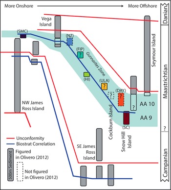

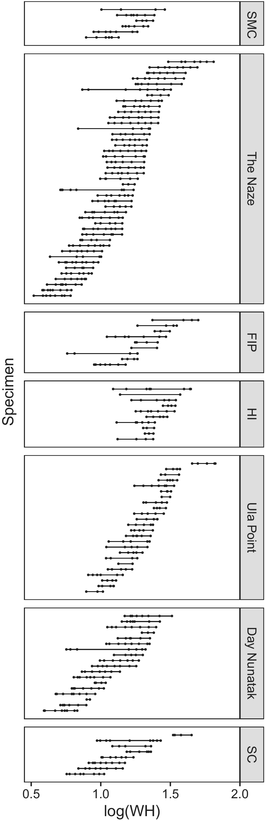
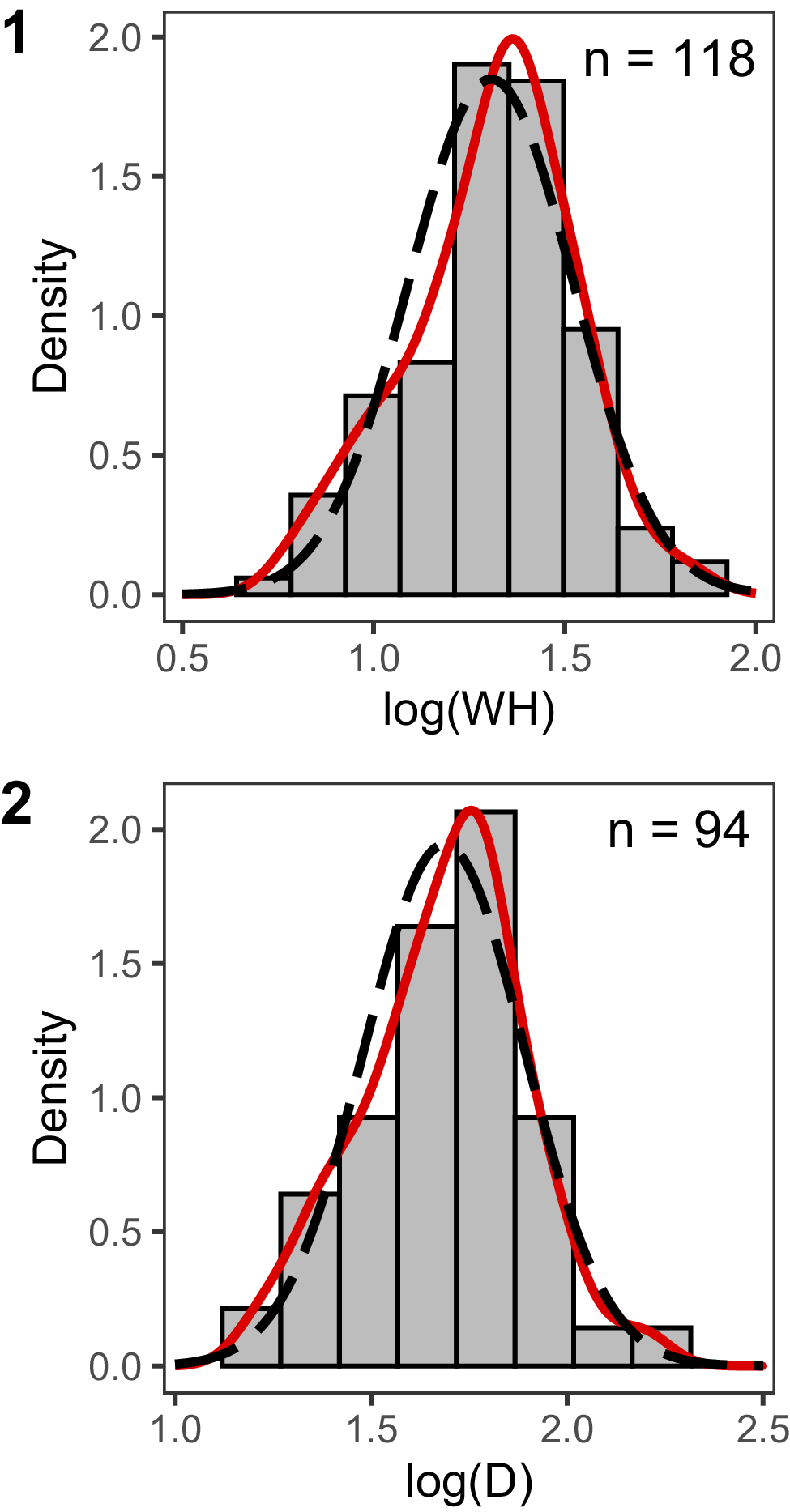
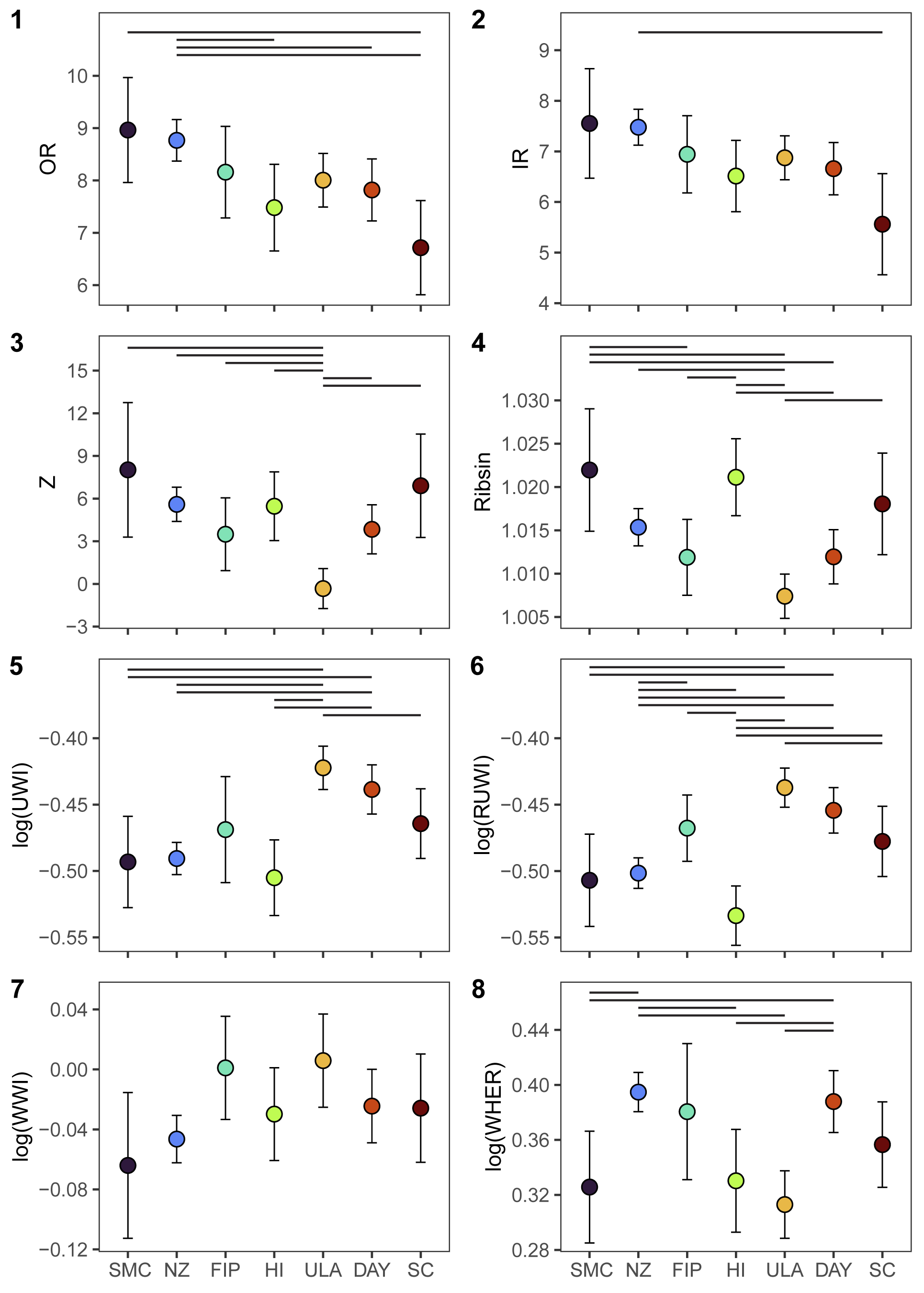
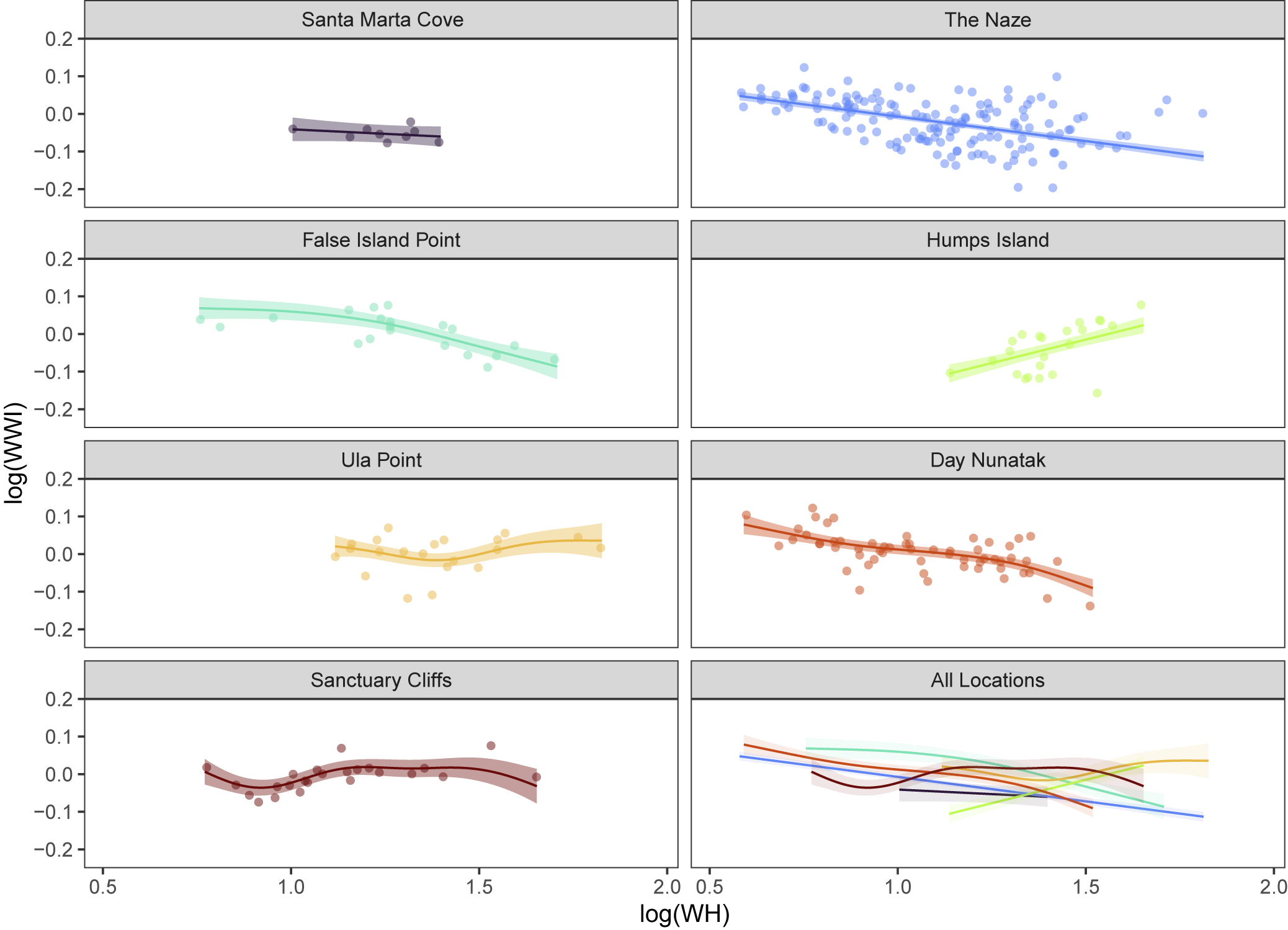

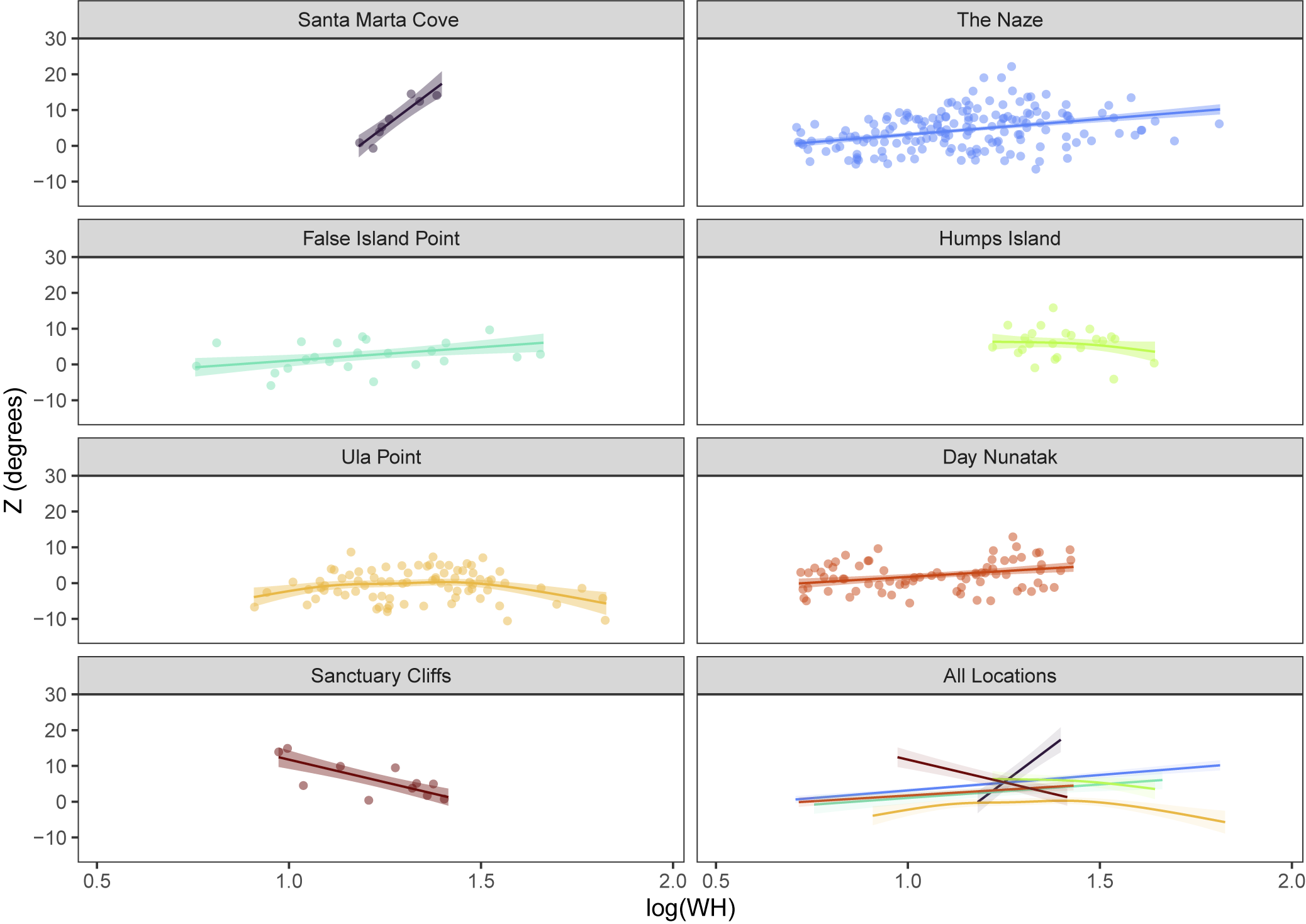

 Open access