Introduction

The role of terrestrial snow cover as a significant geophysical variable influencing climatological and hydrological processes is well documented (e.g. Reference Ross and WalshRoss and Walsh, 1986). Given the dynamic variability of snow cover at the hemispheric (seasonal) to local (daily) space and time-scales, and the need to understand the role of snow cover in climatological, hydrological and modelling studies, consistent and synoptic acquisition of snow-cover information is required. Remote sensing is an ideal source for snow-cover data because this technology can provide quantitative, repetitive and spatially continuous observations of large regions. It is impossible to acquire this level of information using surface sampling. While optical satellite imagery has provided a long time series of snow-extent data that has proven very useful for a variety of climatological studies (e.g. Reference Frei and RobinsonFrei and Robinson, 1999), passive-microwave imagery has some notable characteristics that create particular potential.

These benefits include all-weather imaging capabilities, rapid scene-revisit time and the ability to retrieve quantitative information on snow-cover parameters through the estimation of snow water equivalent (SWE). These qualities have led to a significant research effort in developing SWE retrieval algorithms for passive-microwave data (e.g. Reference Chang, Foster and HallChang and others, 1990; Reference Goodison, Walker, Choudhury, Kerr, Njoku and PampaloniGoodison and Walker, 1995; Reference TaitTait, 1998; Reference Pulliainen and HallikainenPulliainen and Hallikainen,2001). The Meteorological Service of Canada (MSC) has developed a series of SWE retrieval algorithms for central Canada, based on the vertically polarized difference index for the 19 and 37 GHz channels of the Special Sensor Microwave/Imager (SSM/I). Separate algorithms derive SWE for open environments, deciduous, coniferous and sparse forest cover. A final SWE value represents the area-weighted average based on the proportional land cover within each pixel. Imagery based on these algorithms (and those previously developed at MSC) has been used since 1988 on a near-real-time, operational basis by agencies responsible for water-resource management across the Canadian Prairies (Reference Goodison, Walker, Choudhury, Kerr, Njoku and PampaloniGoodison and Walker, 1995). The objectives of this study are to utilize the growing time series of passive-microwave-derived data in two ways:

(1) Five-day averaged (pentad) passive-microwave-derived SWE imagery for the winter season (December, January, February) of 1994/95 is compared to a network of in situ SWE measurements throughout central Canada in order to evaluate MSC algorithm performance. The MSCalgorithms were developed and validated through airborne microwave and localized ground-based field campaigns (Reference Goita, Walker, Goodison and ChangGoita and others, 1997). This study represents the first evaluation of the algorithms using a time series of readily available surface SWE data collated from a spatially distributed network. Specific questions include: Does fractional land-cover composition affect algorithm performance? Is there a systematic bias towards over- or underestimation of SWE compared to in situ data?

(2) Ten winter seasons (1988/89 through 1997/98) of SWE imagery are subjected to a rotated principal-component analysis (PCA) to identify the dominant spatial modes of central North American SWE, and the frequency with which these patterns appear. Interpretation of the component-loading patterns will indicate whether regional trends in SWE variability are evident through the SSM/I time series.

Data

The ability to determine terrestrial SWE in the microwaveportion of the electromagnetic spectrumis a function of changes in the scattering of microwave radiation caused by the presence of snow crystals. For a snow-covered surface, brightness temperature, a measure of microwave emission, decreases with increasing snow depth and density because the greater number of snow crystals provides increased scattering of the microwave signal. However, a range of physical parameters, presented in Table 1, complicate this simple relationship.

Table 1.

Parameters influencing interaction between microwave energy and the snowpack

SWE algorithm development at MSC was initiated in the early 1980s, with an airborne and ground-based measurement campaign in the prairie region of western Canada. This led to the development of a dual-channel, open Prairie SWE algorithm applicable to Scanning Multichannel Microwave Radiometer (SMMR; 1978–87), and later SSM/I (1987–present) brightness temperatures. A full description of algorithm development, evaluation and application is provided in Reference Goodison, Walker, Choudhury, Kerr, Njoku and PampaloniGoodison and Walker (1995). A wet-snow indicator, derived from the 37 GHz polarization difference, complements this algorithm (Reference Walker and GoodisonWalker and Goodison, 1993). The SWE imagery produced by this algorithm has proven useful for near-real-time monitoring of Prairie SWE by water-resource management agencies (Reference Goodison, Walker, Choudhury, Kerr, Njoku and PampaloniGoodison and Walker, 1995), and time-series analysis of central North American SWE patterns for climatological applications (e.g. Reference Derksen, LeDrew and GoodisonDerksen and others, 2000b). Given the large area of high-latitude North American land area that is covered by boreal forest, however, there exists a clear need for SWE retrieval algorithms developed specifically for this type of surface cover.

Towards this end, airborne passive-microwave data were collected over the Canadian provinces of Saskatchewan and Manitoba as part of the Boreal Ecosystem–Atmosphere Study (BOREAS) winter 1994 field campaign (Reference ChangChang and others, 1997). Ground surveys to determine snow characteristics including SWE were performed along the flight-lines. Land-cover information was derived from Landsat Thematic Mapper and Advanced Very High Resolution Radiometer (AVHRR) imagery, while SSM/I brightness temperatures were acquired in the Equal-Area SSM/I Earth Grid (EASE-Grid) projection (Reference Armstrong and BrodzikArmstrong and Brodzik, 1995). Together, these data allowed development of individual SWE algorithms, scaled to satellite imagery, for various classes of land cover. Reference Goita, Walker, Goodison and ChangGoita and others (1997) illustrate the relationship between SWE in broad land-cover classes (coniferous, deciduous, sparse forest and open environments) and the 37 – 19 vertically polarized difference index. It is important to note that channel brightness temperatures are co-located, although the microwave emission recorded at 19GHz is taken from a larger field of view (approximately 50 km) and re-sampled. Given the unique linear relationships between the difference index and SWE for the various types of land cover, separate algorithms were derived for each class. Total perpixel SWE is the sum of the SWE values obtained from each land-cover algorithm weighted by the percentage land-cover type (F) within each pixel:

(1)

where subscripts D, C, S and O represent deciduous forest, coniferous forest, sparse forest and open Prairie environments, respectively. Per-pixel land-cover fractions are taken from the International Geosphere–Biosphere Program (IGBP) 1km AVHRR global land-cover dataset (Reference LovelandLoveland and others, 2000) scaled to the 25 km resolution EASE-Grid pixels.

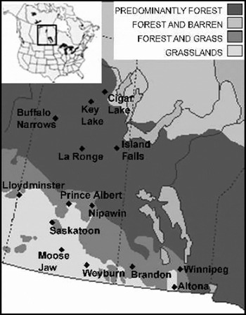
The first phase of this study will compare microwave-estimated SWE with in situ estimates taken from the MSC digital archive of Canadian station snow-depth data. The snow-depth values were converted to SWE using the regionally and seasonally averaged snow-density values provided in Reference BrownBrown (2000). Figure 1 illustrates the network of Canadian stations to be used in the subsequent comparison. Stations were selected to characterize a range of proportional land covers (from 100% open to 100% forested), and winter-season snow-cover regimes (continuous vs non-continuous snow cover). The winter season of 1994/95 will be the focus as this is the most recent complete season of data for many stations of interest. This comparison differs from previous evaluations of the MSC algorithms as it (1) does not utilize intensive field-survey data from a localized region but rather spatially distributed archive data, and (2) investigates a relatively long temporal sequence of data.

Fig. 1.

Stations for which SWE was derived from in situ measurements.

Comparison Of Surface And Ssm/I-Derived Swe

For the 1994/95 season, pentad SWE estimates derived from morning overpass SSM/I brightness temperatures (SWE_SSM/_I) using the MSC algorithms were compared to surface SWE measurements for the stations shown in Figure 1 (SWE_SURFACE). The EASE-Grid pixels with the latitude and longitude coordinates nearest the station location were used for comparison.

As with all point-to-area comparisons, this is an imperfect exercise with some clear limitations. The SWE_SURFACE sample may be unrepresentative of the snow-cover characteristics of the surrounding area captured by the 625 km² resolution EASE-Grid SWE imagery. The SWE_SURFACE pentad measurement is an average of five daily snow-depth observations converted to SWE, while the SWE_SSM/_I measurement is derived using brightness temperatures from a variable number of orbital swaths within a pentad. Given, therefore, the difference in spatial and temporal resolution between the two datasets, only an approximate comparison will result. Still, insight into passive-microwave algorithm performance can still be achieved, especially given the seasonal period of comparison. For instance, do the two SWE datasets capture a similar seasonal cycle of snow accumulation and ablation events even if the magnitude of SWE is sometimes dissimilar?

As an initial comparison of the datasets, correlation values (r) and mean bias error (MBE) were calculated (Table 2). The consistently strong and positive correlation results indicate that the datasets capture a similar seasonal SWE evolution independent of land cover. An increase in SWE_SURFACE is matched with an increase in SWE_SSM=_I and vice versa. These results do not confirm any similarity in SWE magnitude between the datasets, as a strong correlation can exist independent of absolute values. The MBE results, however, do provide insight into dataset agreement, and are also generally favorable. MBE values range from a high of 36.2 mm at Island Falls to a low of 3.1 mm at Buffalo Narrows, and indicate that microwave estimates tend to fall within ±10–20mm, as noted in a previous study by Reference Goodison, Walker, Choudhury, Kerr, Njoku and PampaloniGoodison and Walker (1995). Closer investigation of a number of specific sites highlights some important characteristics of algorithm performance.

Table 2.

Summary of comparison between surface and SSM/I SWE estimates. Land covers (C, coniferous; D, deciduous; S, sparse; O, open) are in per cent

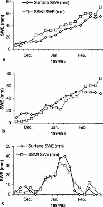
1. The prairie region of North America has little physical relief, and land use is largely agricultural. Winter-season land cover is composed of fallow, stubble, pasture and natural prairie fields. Temperatures tend to remain cold over the Canadian Prairies, although winter-season melt and refreeze events do occur, complicating the relatively simple microwave scattering environment. In open Prairie areas, consistent SWE over- or underestimation by the MSC algorithm exists within individual stations (Fig. 2a and b), but one direction of bias is not systematically observed for all Prairie stations. Importantly, the MSC algorithm reasonably captures periods of snow-free land in the marginal Prairie snow-cover zone (Fig. 2c). Given the large EASE-Grid pixel size relative to each station point, it is not surprising that the algorithm notes some snow even when the point surface measurement does not, due to patchy within-pixel snow cover.

Fig. 2.

Comparison plots for open Prairie stations with continuous snow cover: (a) Altona, (b) Winnipeg and (c) MooseJaw.

2. Algorithm performance in areas with mixed land cover is fundamentally problematic with the MSC scheme. The final per-pixel SWE values are a weighted average of the SWE estimates from the different land-cover algorithms. If a pixel has 50% conifer cover and 50% open environment, neither the conifer nor the open algorithm will retrieve an accurate SWE value for that pixel. While the weighted average proportionally balances the different SWE estimates, it does not necessarily produce a meaningful and accurate SWE value in this context. The MSC algorithm performance should, therefore, be most accurate for pixels with relatively homogeneous land cover. Data from Nipawin (Fig. 3) illustrate the problems in determining SWE in mixed land-cover areas. Dataset disagreement takes the form of both divergent trends in SWE during December, and missed melt and accumulation events in January and February.

Fig. 3.

Comparison plot for a mixed land-cover location (Nipawin).

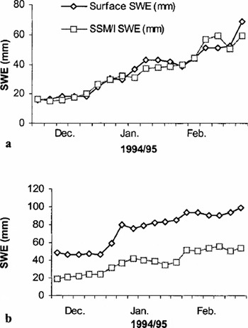
3. Island Falls and Buffalo Narrows are both located in heavily forested regions. The seasonal SWE evolution is accurately captured at both sites (r = 0.94 and 0.96, respectively), but systematic underestimation is a problem at Island Falls (Fig. 4a; MBE = 36.2 mm) but not at Buffalo Narrows (Fig. 4b; MBE = 3.1mm). Underestimation, while not as severe as at Island Falls, also occurs at other forested sites such as Key Lake and La Ronge.

Fig. 4.

Comparison plots for two high-proportion conifer-forest stations: (a) Buffalo Narrows and (b) Island Falls.

Why is algorithm performance accurate for some forested areas (i.e. Buffalo Narrows, Cigar Lake) and not others (Island Falls, Key Lake, La Ronge)? Reference Foster, Chang, Hall and RangoFoster and others (1991) estimate that crown density is too high in 25% of Northern Hemisphere forested regions to allow accurate microwave measurements of surface SWE. Information from the Canadian Forest Service indicates that Island Falls and La Ronge are located in regions of peak conifer volume in the boreal zone, while Buffalo Narrows and Cigar Lake are located in areas of low conifer volume. Other explanatory variables include the presence of small lakes in the region that influence microwave emissivity. Finally, the regional density values used to convert in situ snow depth to SWE may not be representative of a high-density forest environment due to site location, potentially contributing to disagreement between the two datasets.

In summary, comparison of the SWE_SSM/_I and SWE_SURFACE datasets shows that the microwave data characterize a similar seasonal snow-cover regime regardless of land cover. Although periods of disagreement, underestimation and overestimation are evident, SWE imagery derived using the MSC algorithms is composed of reasonable SWE estimates, making it suitable for time-series analysis.

Time-Series Analysis Of Ssm/I-Derived Swe Imagery

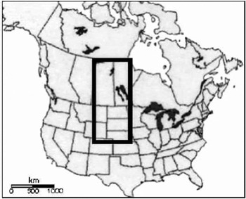
SWE imagery, for a central North American study area (see Fig. 5) and spanning 10 winter seasons (December–February 1988/89–1997/98), was derived from SSM/I brightness temperatures at a temporal resolution of 5 days. Only data from morning overpasses were used, given the higher likelihood of cold, dry snowpack conditions at this time of day (Reference Derksen, LeDrew, Walker and GoodisonDerksen and others, 2000a). Eighteen pentads extend from 2 December to 29 February/1 March as outlined in Table 3. Table 4 summarizes the missing pentads from the time series, which can be attributed to incomplete Prairie coverage within a pentad. Given the errors in determining SWE with microwave data when the snowpack is wet (Reference Walker and GoodisonWalker and Goodison, 1993), surface temperature data were used to identify pentads with regional melt events. While not omitted from the time-series analysis, these pentads are noted in Table 4, and will not be used for data visualization. From the original SWE time series, change in SWE(hereafter referred to as ΔSWE) imagery was calculated by subtracting each SWE pattern from the previous pentad. Analysis of a Prairie-region ΔSWE time series has proven advantageous compared to SWE imagery, due to reduced seasonality of the dominant SWE patterns (Reference Derksen, LeDrew and GoodisonDerksen and others, 2000c).

Fig. 5.

Study area for time-series analysis.

Table 3.

Summary of pentad structure

Table 4.

Pentads omitted from the Δ SWE time series

A rotated (varimax) PCA of the ΔSWE imagery was performed to characterize the dominant spatial modes of variability. The PCA input matrix was composed of columns for each time-series pentad, while SSM/I pixels comprised the rows. The matrix dimensions were 167 (13 missing pentads; see Table 4) columns by 3880 rows (97640 pixel study area = 3880 pixels). Reference Overland and PreisendorferOverland and Preisendorfer (1982) suggest that the use of a correlation matrix is advantageous in isolating spatial variation and oscillation, and the PCA performed in this study utilizes this method.

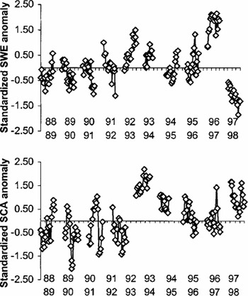
Given that the seasons in this study span a period of marked increase in global temperatures (Reference Karl, Knight and BakerKarl and others, 2000), a change in the frequency of the leading SWE patterns is of interest with regard to the impacts of global climate change. While an examination of SSM/I-derived total study-area SWE and snow-covered area (SCA) anomalies based on the 10-season mean and standard deviation shows no clear trend (Fig. 6), changes in the frequency of appearance of specific spatial patterns of SWE may occur which are not captured by these regional anomalies. These changes can be determined by examining the component-loading patterns.

Fig. 6.

Total study-area SWE (top) and SCA (bottom) anomalies from the passive-microwave-derived SWE time series.

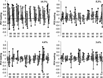
The component loadings indicate the correlation between each component and input spatial patterns on a scale of –1 to ‡1. A high positive loading means the pentad data are similar to the component; a negative loading indicates an inverse spatial pattern between the original data and the component. A loading near zero means there is little similarity. Atime-series plot of the loadings for a given component can therefore be interpreted as an indicator of the temporal frequency of that given spatial mode through the time series. The component-loading patterns for the four leading ΔSWE components are shown in Figure 7. Solid black symbols are used to depict those pentads with a loading greater than 1 standard deviation from the mean of each component phase. These pentads will be used to create the composite patterns for visualization purposes. Some pentads have a strong loading but are not marked with a solid symbol because these intervals (see Table 4) contain regional melt events that adversely influence microwave SWE estimates. Lower-ranked components are not considered further in this study because of generally weak loadings.

Fig. 7.

Loading plots for the four leading Δ SWE components. Variance explained by each component is noted. Solid black symbols indicate those pentads with a loading greater than 1 standard deviation from the mean for each component phase.

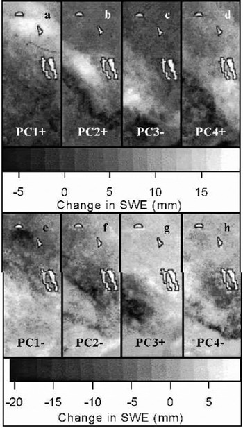
The composite component patterns are shown in Figure 8. Two groupings are evident, with patterns characterizing accumulation events (Fig. 8a–d) and ablation events (Fig. 8e–h). These patterns identify accumulation and ablation zones that occur in the north (PC1), central (PC2), southwest (PC3) and southeast (PC4) parts of the study area.

Fig. 8.

Δ SWE component patterns for accumulation patterns (a–d) and ablation patterns (e–h).

While the interannual variability in ΔSWE component frequency is clearly shown in Figure 8, no trends are evident. Still, compared to one-dimensional regional anomalies (such as those shown in Figure 6) the ΔSWE PCA results represent an enhanced characterization of central North American snow-cover conditions during the SSM/I time series. Consideration of the temporal frequency of the dominant spatial modes of ΔSWE can now serve as the foundation for future studies linking these surface patterns to atmospheric circulation.

Conclusions And Discussion

This study has illustrated the accuracy of the MSC land-cover-sensitive algorithms in estimating winter-season SWE. Comparison of a distributed network of in situ measurements to passive-microwave measurements through a complete winter season yields the following conclusions on algorithm performance:

Strong correlations and moderate MBE values between the surface and microwave datasets were found for the 14 Canadian stations examined in this study. Given that these stations characterize a range of land-cover proportions and seasonal snow-cover regimes, imagery derived using the MSC algorithm was deemed suitable for time-series analysis.

Total study-area SWE and SCA anomalies based on the SSM/I time series through 1998 do not indicate any sustained trends in central North American winter-season snow cover. Anomalously positive snow-cover seasons are interspersed with deficit SWE seasons. A rotated PCA characterized four accumulation and four ablation modes that dominate the spatial variability in SWE through the 10 seasons. Likewise, no clear trend in the frequency of these spatial patterns in evident. The eventual integration of SMMR data, however, will extend the time series back to 1978, and will allow for more rigorous trend analysis, of the type presented in this study. The period of sensor overlap between SMMR and SSM/I must be examined, however, to ensure a consistent time series. The impact on algorithm performance of the slightly different radiometric, orbital and spatial characteristics between the two sensors must be identified.

The results of this study allow confidence to be placed in both the operational SWE maps produced by MSC, and time-series analysis of imagery derived with the algorithm. The benefits of working with SWE imagery include added value for hydrological studies, and the opportunity to apply analysis techniques to continuous, quantitative data (as opposed to binary snow-extent charts). Further research is necessary, therefore, to evaluate microwave SWE estimates in the shoulder seasons of autumn and spring. These intervals provide additional challenges given the typical conditions that adversely impact microwave SWE retrieval: snow on a warm ground (autumn) and wet, melting snow (spring).

The imminent launch of the Advanced Microwave Scanning Radiometer (AMSR) on board the NASA Aqua platform should provide continued microwave data at an improved spatial resolution, representing enhanced opportunities for the application of microwave imagery. In short, passive-microwave imagery will continue to contribute towards improved understanding of the role of snow cover in global physical processes.