


1. Introduction
1.1. Frozen hydrometeors in the atmosphere
The settling of heavy particles in air turbulence is relevant to a wealth of natural phenomena, notably including atmospheric processes (Shaw Reference Shaw2003; Grabowski & Wang Reference Grabowski and Wang2013). In particular, the precipitation of frozen hydrometeors (such as ice crystals, hail and snowflakes) plays a crucial role in weather forecasting, prediction of snow accumulation, and climate projections (Khvorostyanov & Curry Reference Khvorostyanov and Curry2002; Hong, Dudhia & Chen Reference Hong, Dudhia and Chen2004; Lehning et al. Reference Lehning, Löwe, Ryser and Raderschall2008; Bodenschatz et al. Reference Bodenschatz, Malinowski, Shaw and Stratmann2010; Radenz et al. Reference Radenz, Bühl, Seifert, Griesche and Engelmann2019; IPCC 2021). Beside the microphysics regulating the hydrometeor formation and evolution, the particle–fluid mechanics that set the fall speed of these complex objects have challenged scientists for decades (Locatelli & Hobbs Reference Locatelli and Hobbs1974; Böhm Reference Böhm1989; Mitchell Reference Mitchell1996; Heymsfield & Westbrook Reference Heymsfield and Westbrook2010; Pruppacher & Klett Reference Pruppacher and Klett2010; Tagliavini et al. Reference Tagliavini, McCorquodale, Westbrook, Corso, Krol and Holzner2021a). Several seminal laboratory studies have investigated the problem using replicas of frozen hydrometeors falling in quiescent environments, typically in liquids (List & Schemenauer Reference List and Schemenauer1971; Field et al. Reference Field, Klaus, Moore and Nori1997; Westbrook & Sephton Reference Westbrook and Sephton2017; McCorquodale & Westbrook Reference McCorquodale and Westbrook2021a,Reference McCorquodale and Westbrookb). The extension of such results to the actual conditions in the turbulent atmosphere is not straightforward, for two main reasons. First, the much smaller density ratio in liquid–solid systems does not allow for a full dynamic similarity (Bagheri & Bonadonna Reference Bagheri and Bonadonna2016; Westbrook & Sephton Reference Westbrook and Sephton2017; Tinklenberg, Guala & Coletti Reference Tinklenberg, Guala and Coletti2023). Second, ambient turbulence plays a crucial role for both the settling rate and the spatial distribution (Garrett & Yuter Reference Garrett and Yuter2014; Nemes et al. Reference Nemes, Dasari, Hong, Guala and Coletti2017; Li et al. Reference Li, Lim, Berk, Abraham, Heisel, Guala, Coletti and Hong2021a,Reference Li, Abraham, Guala and Hongb). Crucially, the air flow fluctuations not only amplify the variance of the settling velocity of frozen hydrometeors (which is already large due to their spectrum of size, shape and density), they also impact their average fall speed. The present work focuses on this second aspect, particularly for the class of hydrometeors known as plate crystals. Classifications of frozen hydrometeors indicates that graupel (heavily rimed aggregates) may be approximated as round/spherical, needle crystals as slender cylinders, and plate crystals as thin disks (Magono & Lee Reference Magono and Lee1966; Li, Guala & Hong Reference Li, Guala and Hong2023).
1.2. Particles settling in turbulence
For solid spheres in turbulence, the key variables influencing the settling include the solid-to-fluid density ratio,  $\tilde {\rho }=\rho _p/\rho _f$, the particle diameter $D$ normalized by the Kolmogorov length scale $\eta$ of the ambient turbulent flow, $D/\eta$, and the particle volume fraction $\varPhi _V$ (Brandt & Coletti Reference Brandt and Coletti2022). Additional parameters have been used to describe the prevalence of mechanisms that may enhance or reduce the settling rate. In particular, the Stokes number $St=\tau _p/\tau _i$ compares the particle response time $\tau _p$ and a characteristic time scale of the turbulence $\tau _i$ (typically taken as the Kolmogorov time scale $\tau _{\eta }$ or the integral time scale $\tau _L$) (Aliseda et al. Reference Aliseda, Cartellier, Hainaux and Lasheras2002; Shaw Reference Shaw2003; Petersen, Baker & Coletti Reference Petersen, Baker and Coletti2019). Similarly, the settling velocity parameter $Sv$ is the ratio between the settling velocity of an isolated particle in quiescent fluid, $V_{t,0}$, and a velocity scale of the turbulence: $Sv_{\eta }=V_{t,0}/u_{\eta }$ and $Sv_L=V_{t,0}/u'$, based on the Kolmogorov velocity $u_{\eta }$ and the root mean square (r.m.s.) velocity fluctuation $u'$, respectively. To characterize the inertia of the fluid flow relative to the particle, the Reynolds number $Re=V_t D/\nu$ is commonly used, where $\nu$ is the fluid kinematic viscosity, and $V_t$ is the terminal velocity of the particle. The latter may differ significantly from $V_{t,0}$ due to ambient turbulence and/or collective effects (Balachandar & Eaton Reference Balachandar and Eaton2010; Brandt & Coletti Reference Brandt and Coletti2022).
As summarized by Nielsen (Reference Nielsen1993), even for the seemingly simple case of spherical particles, turbulence may affect the settling velocity via different mechanisms. While tracer-like particles may be trapped in vortices (Tooby, Wick & Isaacs Reference Tooby, Wick and Isaacs1977; Toschi & Bodenschatz Reference Toschi and Bodenschatz2009), inertial ones may preferentially sample the downward moving side of eddies, leading to settling enhancement (Maxey Reference Maxey1987). Such preferential sweeping is generally considered prevalent for particles smaller than or comparable to the dissipative scales of the turbulence, and having  $St_{\eta }$ and $Sv_{\eta }$ of order unity (Wang & Maxey Reference Wang and Maxey1993; Aliseda et al. Reference Aliseda, Cartellier, Hainaux and Lasheras2002; Rosa et al. Reference Rosa, Parishani, Ayala and Wang2016; Baker et al. Reference Baker, Frankel, Mani and Coletti2017; Berk & Coletti Reference Berk and Coletti2021). However, recent laboratory measurements and numerical simulations over wide ranges of turbulence Reynolds numbers $Re_{\lambda }$ (where $\lambda$ is the Taylor microscale) indicated that preferential sweeping can act over a broad range of scales (Petersen et al. Reference Petersen, Baker and Coletti2019; Tom & Bragg Reference Tom and Bragg2019). This was confirmed indirectly by field studies that performed large-scale imaging on frozen hydrometeors of approximately round shape (Nemes et al. Reference Nemes, Dasari, Hong, Guala and Coletti2017; Li et al. Reference Li, Lim, Berk, Abraham, Heisel, Guala, Coletti and Hong2021a,Reference Li, Abraham, Guala and Hongb). Opposite to preferential sweeping, loitering refers to a particle spending more time in upward-moving regions of turbulent eddies, hindering the settling, which may occur for relatively high fall speeds ( $Sv_L>1$; Good et al. Reference Good, Ireland, Bewley, Bodenschatz, Collins and Warhaft2014). Finally, for $Re \gg 1$, the nonlinear relation between the drag force and the particle–fluid slip velocity implies that the settling is hindered by upward fluctuations more than enhanced by downward ones. This can cause a net reduction of settling velocity for heavy particles (Tunstall & Houghton Reference Tunstall and Houghton1968; Mei, Adrian & Hanratty Reference Mei, Adrian and Hanratty1991; Wang & Maxey Reference Wang and Maxey1993; Bagchi & Balachandar Reference Bagchi and Balachandar2003; Homann, Bec & Grauer Reference Homann, Bec and Grauer2013; Good et al. Reference Good, Ireland, Bewley, Bodenschatz, Collins and Warhaft2014; Fornari et al. Reference Fornari, Picano, Sardina and Brandt2016b; Chouippe & Uhlmann Reference Chouippe and Uhlmann2019; Singh, Pardyjak & Garrett Reference Singh, Pardyjak and Garrett2023) as well as a reduction of rise velocity for bubbles (Ruth et al. Reference Ruth, Vernet, Perrard and Deike2021).
1.3. Disks settling in turbulence
Plate crystals are among the most abundant types of frozen hydrometeors (Pruppacher & Klett Reference Pruppacher and Klett2010), and understanding their behaviour has motivated a large number of studies on falling disks. The pioneering laboratory work of Willmarth, Hawk & Harvey (Reference Willmarth, Hawk and Harvey1964) established the use of the inertia ratio  $I^* = I/(\rho _f D^5)$, comparing the disk moment of inertia $I$ (around the central axis parallel to its diameter) to that of the sphere of fluid surrounding it. For a thin disk of thickness $h$,
$h$,  $I^*=({\rm \pi} /64) \tilde {\rho }/\chi$, with the aspect ratio $\chi =D/h$ assumed much larger than unity (Field et al. Reference Field, Klaus, Moore and Nori1997; Auguste, Magnaudet & Fabre Reference Auguste, Magnaudet and Fabre2013; Lau, Huang & Xu Reference Lau, Huang and Xu2018). The parameter $I^*$ has been used to predict the different falling styles in a parameter space along with the Galileo number $Ga=U_g D/\nu$ (Chrust, Bouchet & Dušek Reference Chrust, Bouchet and Dušek2013; Moriche, Uhlmann & Dušek Reference Moriche, Uhlmann and Dušek2021; Moriche et al. Reference Moriche, Hettmann, García-Villalba and Uhlmann2023; Tinklenberg et al. Reference Tinklenberg, Guala and Coletti2023). The convenience of using $Ga$ rather than $Re$ stems from the a priori definition of the gravitational velocity $U_g=\{2\,|\tilde {\rho }-1|\,gh\}^{1/2}$ (where $g$ is the gravitational acceleration), which is a reasonable approximation of $V_t$ if the drag coefficient $C_D$ is of order unity. The mapping of the disk falling style and speed onto the $I^*\unicode{x2013}Ga$ plane (or other equivalent parameter spaces) is a topic of active research.
In general, the settling of non-spherical particles, even in an otherwise quiescent fluid, is a complex process (Ern et al. Reference Ern, Risso, Fabre and Magnaudet2012). The translational and rotational dynamics are greatly simplified when assuming Stokes drag and Jeffery torque (Jeffery Reference Jeffery1922), but this requires a vanishingly small  $Re$. In air, this is a tenable assumption only for microscopic objects. Even in the small- $Re$ limit, the torque due to the fluid inertia becomes important and fundamentally affects the dominant orientation of settling disks (Dabade, Marath & Subramanian Reference Dabade, Marath and Subramanian2015; Gustavsson et al. Reference Gustavsson, Sheikh, Lopez, Naso, Pumir and Mehlig2019). In particular, recent theoretical and numerical studies on disks falling at small $Re$ indicated that inertial torque typically dominates over viscous torque, causing them to fall predominantly with their broad side first (Anand, Ray & Subramanian Reference Anand, Ray and Subramanian2020; Sheikh et al. Reference Sheikh, Gustavsson, Lopez, Lévêque, Mehlig, Pumir and Naso2020). This is consistent with the common assumption that small ice crystals maintain their direction of maximum extension as approximately horizontal (steady falling; see Sassen Reference Sassen1980; Matrosov et al. Reference Matrosov, Reinking, Kropfli, Martner and Bartram2001), although fluttering (back and forth lateral oscillation) and tumbling (continuously turning end-over-end) have also been observed (Kajikawa Reference Kajikawa1992; Mitchell Reference Mitchell1996). Highly resolved simulations have allowed $V_t$ and the associated drag coefficient $C_D$ to be determined for ice crystals at various fixed orientations (Tagliavini et al. Reference Tagliavini, McCorquodale, Westbrook, Corso, Krol and Holzner2021a,Reference Tagliavini, McCorquodale, Westbrook and Holznerb). However, precipitating crystals can produce unstable wakes that oscillate and couple with the object's motion. Indeed, while plate crystals that remain suspended in clouds have sizes of tens to hundreds of microns, ground-based observations show plate crystals of typical diameters $O(1\ {\rm mm})$ and fall speeds $O(1\ {\rm m}\ {\rm s}^{-1})$ (Higuchi Reference Higuchi1956; Ono Reference Ono1969; Auer & Veal Reference Auer and Veal1970; Kajikawa Reference Kajikawa1972; Barthazy & Schefold Reference Barthazy and Schefold2006). In ambient air, this implies $Re = O(100)$, so that unsteady wakes and complex falling styles are expected (Field et al. Reference Field, Klaus, Moore and Nori1997; Ern et al. Reference Ern, Risso, Fabre and Magnaudet2012; Auguste et al. Reference Auguste, Magnaudet and Fabre2013; Moriche et al. Reference Moriche, Uhlmann and Dušek2021).
From the above, it is not surprising that non-spherical particles in turbulence would exhibit very rich dynamics, and several researchers have explored the wide parameter space spanned by such systems (Voth & Soldati Reference Voth and Soldati2017). Oblate (disk-like) particles have been investigated mostly numerically. The settling of disks in homogeneous turbulence, which is the focus of our work, was investigated, among others, by Jucha et al. (Reference Jucha, Naso, Lévêque and Pumir2018), Gustavsson et al. (Reference Gustavsson, Sheikh, Lopez, Naso, Pumir and Mehlig2019), Sheikh et al. (Reference Sheikh, Gustavsson, Lopez, Lévêque, Mehlig, Pumir and Naso2020) and Anand et al. (Reference Anand, Ray and Subramanian2020). These authors assumed Stokes drag and performed detailed analysis of the disk orientation and collision rates. Importantly, the above-mentioned role of inertial torque even in the Stokes drag regime was highlighted. For disks falling at  $Re \gg 1$ (which is expected for precipitating plate crystals, as discussed), the Stokesian assumptions become inapplicable, and accurate numerical simulations require fully resolving the turbulent fluid dynamics at the particle scale. Such particle-resolved direct numerical simulations (PR-DNS) have led to great insight into particle-laden turbulent flows, mostly for spherical particles – e.g. Naso & Prosperetti (Reference Naso and Prosperetti2010), García-Villalba, Kidanemariam & Uhlmann (Reference García-Villalba, Kidanemariam and Uhlmann2012), Tenneti & Subramaniam (Reference Tenneti and Subramaniam2014), Picano, Breugem & Brandt (Reference Picano, Breugem and Brandt2015), Fornari et al. (Reference Fornari, Picano, Sardina and Brandt2016b), Uhlmann & Chouippe (Reference Uhlmann and Chouippe2017) and Peng, Ayala & Wang (Reference Peng, Ayala and Wang2019), among many others – but also for oblate particles (Ardekani et al. Reference Ardekani, Costa, Breugem, Picano and Brandt2017; Wang et al. Reference Wang, Abbas, Yu, Pedrono and Climent2018). The computational cost, however, limits the range of accessible parameters. In particular, compared to conditions relevant to plate crystals, such studies have typically focused on relatively large and weakly oblate particles with relatively low $\tilde {\rho }$ and $Re$, suspended in turbulence of moderate intensity. Moreover, the effect of gravity on oblate particles in turbulence was never considered in PR-DNS studies.
Experimental investigations of disks settling in turbulence are similarly scarce; we are aware of only the work by Byron et al. (Reference Byron, Einarsson, Gustavsson, Voth, Mehlig and Variano2015, Reference Byron, Tao, Houghton and Variano2019) and Esteban, Shrimpton & Ganapathisubramani (Reference Esteban, Shrimpton and Ganapathisubramani2020), both in water. Byron et al. (Reference Byron, Einarsson, Gustavsson, Voth, Mehlig and Variano2015) forced homogeneous steady turbulence in a zero-mean-flow chamber using randomly actuated jets, and investigated particles of size comparable to the Taylor microscale  $\lambda$, including cylinders with $\chi \sim 2$, $\tilde {\rho } = 1.003\unicode{x2013}1.006$ and $Sv_L \sim 0.48\unicode{x2013}1.25$. They reported that turbulence reduced the fall speed by 40 %–60 %, which Fornari, Picano & Brandt (Reference Fornari, Picano and Brandt2016a) and Fornari et al. (Reference Fornari, Picano, Sardina and Brandt2016b) later attributed to a combination of unsteady effects and nonlinear drag. Compared to cylinders with $\chi \sim 0.25\unicode{x2013}1.05$, no influence of the particle shape was observed on the fall speed. On the other hand, Esteban et al. (Reference Esteban, Shrimpton and Ganapathisubramani2020) used a similar set-up to generate homogeneous turbulence, but considered thinner and denser disks, $\chi = 15\unicode{x2013}25$ and $\tilde {\rho }= 2.7$. Their diameter was smaller than $\lambda$ but much larger than $\eta$, and they were dropped at different times in temporally decaying turbulence in order to widen the range of turbulent conditions, $Sv_L = 1.5\unicode{x2013}7$. It was found that the disks reached a settling velocity approximately 20 % higher than in quiescent water, in stark contrast with findings for spherical particles for a similar range of $Sv_L$ (Good et al. Reference Good, Ireland, Bewley, Bodenschatz, Collins and Warhaft2014). This was attributed to their interaction with eddies of similar size, which caused the disks to orient edge-on and accelerate downwards during part of their descent.
1.4. Focus of the present study
To summarize, while precipitating plate crystals in the atmosphere can be approximated as geometrically simple disks, they are associated with a part of the parameter space that poses formidable challenges: their shape is far from spherical, they are much denser than the surrounding fluid, they fall in intense turbulence, and their Reynolds number is much greater than unity. In fact, despite its clear relevance to atmospheric science, this regime has remained virtually unexplored both numerically and experimentally, and the most fundamental questions remain unanswered.
The goal of this paper is to investigate the dynamics of thin disks in homogeneous air turbulence to identify the mechanisms that have a dominant effect on the settling velocity. Disks with properties comparable to precipitating plate crystals are released in two different levels of turbulence that mimic atmospheric conditions. Their behaviour is compared to what we recently reported in quiescent air (Tinklenberg et al. Reference Tinklenberg, Guala and Coletti2023), while also extending the range of the objects’ sizes. Through statistical analysis of thousands of trajectories captured via high-speed imaging, we address the following open questions. Does turbulence increase or decrease the disk settling velocity, and by which mechanisms? Which parameters and spatio-temporal scales best predict when such mechanisms manifest? How does turbulence influence the disk falling styles, and how does this in turn affect the settling rate? The remainder of the paper is organized in the following manner. The experimental methodology is presented in § 2, which includes a description of the facility and turbulence properties (§ 2.1), the characteristics of the disks (§ 2.2), and the experimental and processing techniques (§ 2.3). The presentation of the results in § 3 begins with considerations on the relevant parameter spaces (§ 3.1), before reporting our findings on the disk translational (§ 3.2) and rotational (§ 3.3) motion. We conclude by summarizing and discussing our findings in § 4.
2. Methodology
2.1. Disk properties
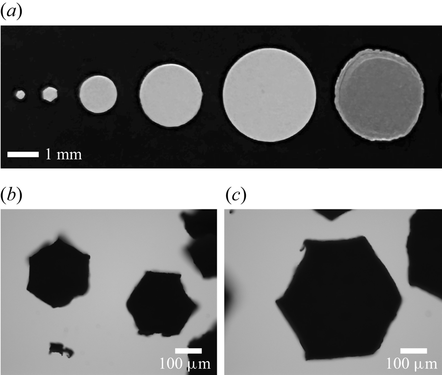
We consider disks with a range of properties comparable to plate crystals in the atmosphere; see figure 1(a). All are made of polyethylene terephthalate (PET,  $\rho _p=1380$ kg m $^{-3}$) with dimensions listed in table 1, where important dimensional and non-dimensional parameters are summarized. The approximate nominal diameter will be used in the labelling of the following figures. The actual diameter is evaluated via standard or microscope imaging depending on the disk size, while the thickness is obtained by caliper measurements as described in Tinklenberg et al. (Reference Tinklenberg, Guala and Coletti2023). Most considered disks are commercially manufactured glitter of thickness $50\,\mathrm {\mu }$m. The thicker 3 mm disks, denoted as 3 mm $^*$, are individually laser cut out of $100\,\mathrm {\mu }$m sheets of PET. The 0.3 and 0.5 mm disks are hexagonal in shape (see figures 1b,c), and we take $D$ as the diameter of the circumscribing circle, as is common in the hydrometeor literature (Böhm Reference Böhm1989; Heymsfield & Westbrook Reference Heymsfield and Westbrook2010).
Images of all disks studied. (a) From left to right,  $D$ increasing from 0.3 mm to 3 mm $^*$. (b) Microscope images of 0.3 mm disks. (c) Microscope images of 0.5 mm disks.
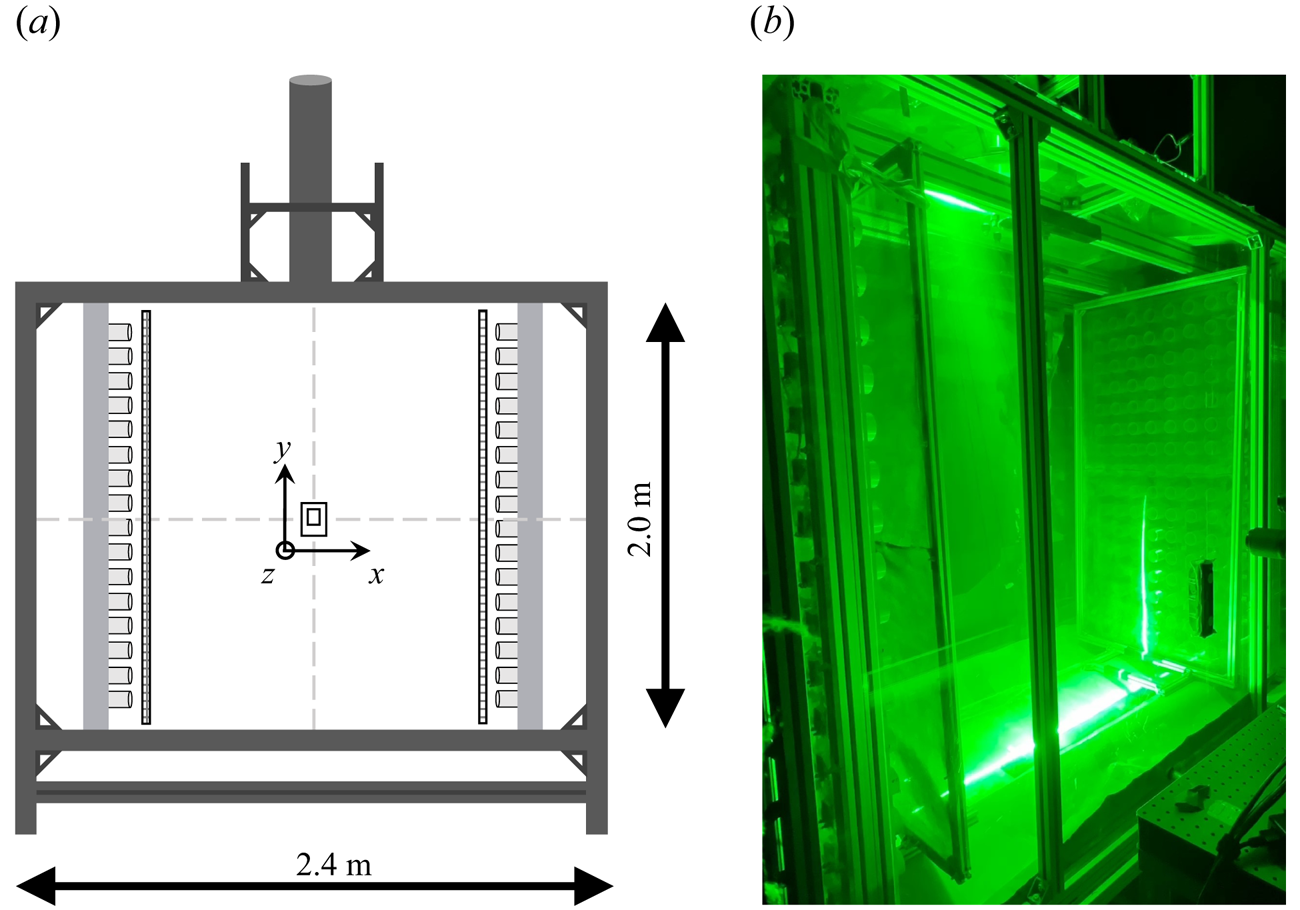
Main dimensional and non-dimensional characteristics of the investigated disks with estimated uncertainties, including disk diameter  $D$, disk thickness $h$, disk aspect ratio $\chi = D/h$, solid-to-fluid density ratio $\tilde {\rho } = \rho _p/\rho _f$, Galileo number $Ga = U_g D /\nu$, where the gravitational velocity is $U_g=\{2|\tilde {\rho }-1|gh\}^{1/2}$, the inertia ratio $I^* = ({\rm \pi} /64) \tilde {\rho }/\chi$, the measured terminal velocity in quiescent air $V_{t,0}$, the Reynolds number calculated as $Re_0 = V_{t,0}D/\nu$, the diameter to turbulent Kolmogorov scales considered $D/\eta$, and the settling velocity number defined based on the integral velocity scale of the turbulence $Sv_L = V_{t,0}/u'$. Uncertainties listed for $D$,
$D$,  $h$ and $V_{t,0}$ are one standard deviation of the measured quantity. For $D$, this was found by measuring calibrated images of a sample of individual disks, whereas $h$ was measured by closing caliper teeth on various stacks of disks and averaging the quantity for each stack. The characteristics for the studies of Byron et al. (Reference Byron, Einarsson, Gustavsson, Voth, Mehlig and Variano2015) and Esteban et al. (Reference Esteban, Shrimpton and Ganapathisubramani2020), calculated from the data reported in those papers, are also listed for comparison.
The non-dimensional parameters will be discussed in detail in § 3. For comparison, we also report the characteristics of the disks considered in the only previous experimental studies that considered disks falling in turbulence, Byron et al. (Reference Byron, Einarsson, Gustavsson, Voth, Mehlig and Variano2015) and Esteban et al. (Reference Esteban, Shrimpton and Ganapathisubramani2020), which highlights the vast differences in the main parameters.
2.2. Turbulence properties
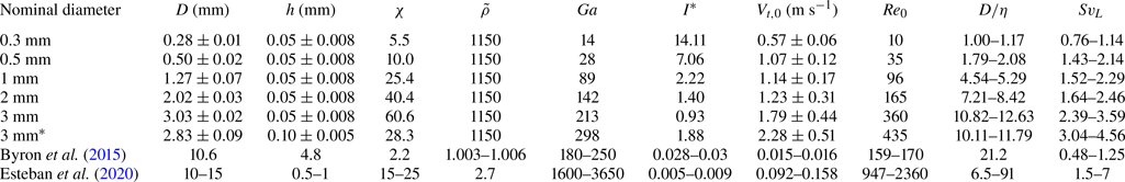
The disks are dropped in a large transparent chamber ( $2.4\times 2\times 1.1$ m3), shown in figure 2, where turbulence is generated via two vertical panels facing each other at 1.81 m apart. Each panel contains 128 nozzles in planar arrays of $8\times 16$. Each nozzle is connected to a pressurized air line at 700 kPa, and attached to computer-controlled solenoid valves, which are actuated to issue jets in randomized sequence following the sun-bathing algorithm proposed by Variano & Cowen (Reference Variano and Cowen2008). The jets create approximately homogeneous air turbulence with negligible mean flow over a central region of size $O(1\ {\rm m}^{3})$. The strength of the turbulence fluctuations is adjusted by controlling the mean firing time of the jets, as well as adding square-mesh grids in front of the jet arrays. The facility was previously characterized in detail (Carter et al. Reference Carter, Petersen, Amili and Coletti2016; Carter & Coletti Reference Carter and Coletti2017, Reference Carter and Coletti2018) and has been used extensively to study the interaction of homogeneous turbulence with small spherical particles (Petersen et al. Reference Petersen, Baker and Coletti2019; Berk & Coletti Reference Berk and Coletti2021; Hassaini & Coletti Reference Hassaini and Coletti2022; Hassaini, Petersen & Coletti Reference Hassaini, Petersen and Coletti2023).
(a) Experimental turbulence chamber schematic indicating chute entrance and jet arrays with optional grids placed in front. Central imaging region shown for the large field of view, with the inset small field of view and definition of the global axes. (b) Image of the experimental chamber with laser sheet and grids.
Two configurations of the chamber are considered here: one with square-mesh grids placed in front of the jets and attenuating their strength, and one that does not employ grids. The main characteristics of both cases, which we will refer to generically as ‘weaker turbulence’ and ‘stronger turbulence’, are summarized in table 2. As in other similar facilities (e.g. Esteban et al. Reference Esteban, Shrimpton and Ganapathisubramani2020), the planar symmetry of the jet arrays leads to a large-scale anisotropy (LSA) defined by the ratio between the r.m.s. fluctuations parallel and normal to the jet axes,  ${\rm LSA} = u_x'/u_y' = u_x'/u_z'$. Here and in the following, $x$ and $y$ indicate the horizontal and vertical upward directions, respectively. Following Carter et al. (Reference Carter, Petersen, Amili and Coletti2016), we define $u' = (u_x'+2 u_y')/3$. Alternative averaging strategies lead to marginal differences. The integral scales $L$ and thus the Taylor-microscale Reynolds number $Re_{\lambda }$ are much smaller than in the atmosphere, though sufficient for the emergence of an inertial sub-range with classic power-law scaling (Carter & Coletti Reference Carter and Coletti2018). The limitation on $Re_{\lambda }$ is typical of laboratory set-ups, apart from facilities in which low-viscosity fluids are used (e.g. Zagarola & Smits Reference Zagarola and Smits1998; De Graaff & Eaton Reference De Graaff and Eaton2000; Küchler, Bewley & Bodenschatz Reference Küchler, Bewley and Bodenschatz2023). In those, however, the spatial limitation on the integral scale, combined with the need to achieve high levels of turbulent Reynolds numbers, translates into microscopic Kolmogorov scales, orders of magnitude smaller than in the atmosphere (where $\eta = O(1\ {\rm mm})$; Shaw Reference Shaw2003). In the present study, while the dissipation rate $\epsilon$ is higher than typical levels in clouds (Grabowski & Wang Reference Grabowski and Wang2013), $\eta$ is still comparable to that encountered in the atmospheric surface layer through which hydrometeors precipitate (see e.g. the field studies by Li et al. Reference Li, Lim, Berk, Abraham, Heisel, Guala, Coletti and Hong2021a, where $\eta \sim 0.5$ mm). The r.m.s. velocity fluctuations $u'$ yield realistic values of $Sv_L$ (see e.g. Nemes et al. (Reference Nemes, Dasari, Hong, Guala and Coletti2017) and Li et al. (Reference Li, Lim, Berk, Abraham, Heisel, Guala, Coletti and Hong2021a), where $Sv_L=0.60\unicode{x2013}10.7$). This parameter, whose inverse is sometimes referred to as turbulence intensity, is expected to be influential for the settling dynamics (Wang & Maxey Reference Wang and Maxey1993; Good et al. Reference Good, Ireland, Bewley, Bodenschatz, Collins and Warhaft2014; Byron et al. Reference Byron, Einarsson, Gustavsson, Voth, Mehlig and Variano2015; Fornari et al. Reference Fornari, Picano and Brandt2016a,Reference Fornari, Picano, Sardina and Brandtb; Petersen et al. Reference Petersen, Baker and Coletti2019). Lower turbulence intensities (with comparable $L$ but smaller $u'$) have been explored, yielding marginal effects on the disk motion that are not reported here.
Turbulence characterization for cases considered. Kolmogorov scales  $u_{\eta }$, $\eta$, $\tau _{\eta }$ (velocity, length, time), Taylor microscale $\lambda$ (length), integral scales $u'$,
$u'$,  $L$,
$L$,  $\tau _L$ (velocity, length, time), dissipation $\varepsilon$, and Reynolds numbers calculated as $Re_{\lambda } = u' \lambda /\nu$ and $Re_L = u' L/\nu$. Weaker turbulence corresponds to G6 forcing, with grids in place, and stronger turbulence corresponds to B6 forcing, as in Carter et al. (Reference Carter, Petersen, Amili and Coletti2016).

2.3. Experimental and processing methods
A detailed description of the facility operation and imaging techniques as well as the post-processing methods was provided in Petersen et al. (Reference Petersen, Baker and Coletti2019) and Tinklenberg et al. (Reference Tinklenberg, Guala and Coletti2023), and are briefly summarized here. The random-jet forcing is run for sufficient time to allow the homogeneous region of turbulence to reach a statistically stationary state, and is sustained throughout the duration of the experiment. Disks are released from a sieve shaker into the chamber via a 3 m long chute routed through its ceiling, and fall in it for approximately 1 m before reaching the imaging field of view. This ensures they are observed in their ‘saturated path’, i.e. having reached a dynamic equilibrium with the flow and therefore displaying a behaviour statistically independent of the vertical distance  $y$ (Esteban et al. Reference Esteban, Shrimpton and Ganapathisubramani2020).
The sieve mesh size and shaker settings for each disk type are selected to maintain a volume fraction  $\varPhi _V = O(10^{-5})$, as verified by counting the disks in the imaged volume. Varying the concentration in separated tests confirms that the level of dilution is sufficient to neglect pairwise interactions or other collective effects that may influence the observables. The vertical imaging plane at the centre of the chamber is illuminated with a 3 mm thick laser sheet and captured via two high-speed cameras operated at 4300 Hz. Each CMOS camera (Phantom VEO 640) captures a different size window, which we refer to as the large field of view (LFV) and small field of view (SFV), the latter being a sub-region of the former. The LFV employs a 105 mm Nikon lens and is $11.2\ {\rm cm}\times 8.4\ {\rm cm}$ with 11.4 pixels mm $^{-1}$. The SFV is captured using a 200 mm Nikon lens and is $4.8\ {\rm cm}\times 3.6\ {\rm cm}$ with 26.6 pixels mm $^{-1}$. For the sub-millimetre disks, the SFV data is used to maintain higher pixel/diameter ratio. For the disks with $D \geq 1$ mm, the LFV data allow us to capture longer trajectories while still warranting sufficient resolution to determine the disk location and orientation. To increase statistical convergence and limit the effect of run-to-run variability, a minimum of five experimental runs is performed for each disk size and turbulence level.
Disks are identified in a binarized form of the images, and filtered based on their size, intensity and sharpness. Out-of-focus objects are removed based on the image intensity gradient obtained by Sobel approximation. Ellipses are fit to each disk to obtain sub-pixel-accurate centroid location and orientation of the major axis. At the present volume fraction, the probability that two or more disk images overlap is minimal. If this occurs, then the disk images appear out of focus and/or exceed the expected size of the ellipse fit, and the rare instances are discarded. The ellipse fit is used to reconstruct the three-dimensional orientation of the disks, obtaining the orientation unit vector  $\hat {\boldsymbol {p}}$ (the disk axis of rotational symmetry) following Baker & Coletti (Reference Baker and Coletti2022). Sign ambiguities are resolved by enforcing a minimum angular acceleration condition. The application of this constraint is trivial, as the angular acceleration associated with a spurious sign change of $\hat {\boldsymbol {p}}$ is typically more than one order of magnitude above the average. The centroid trajectories and disk orientations are convolved in time with a Gaussian kernel to obtain smoothed positions, velocities and angular velocities.
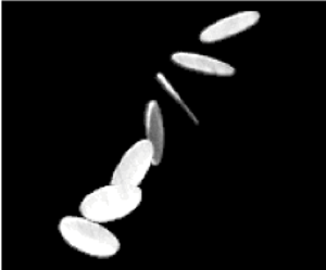
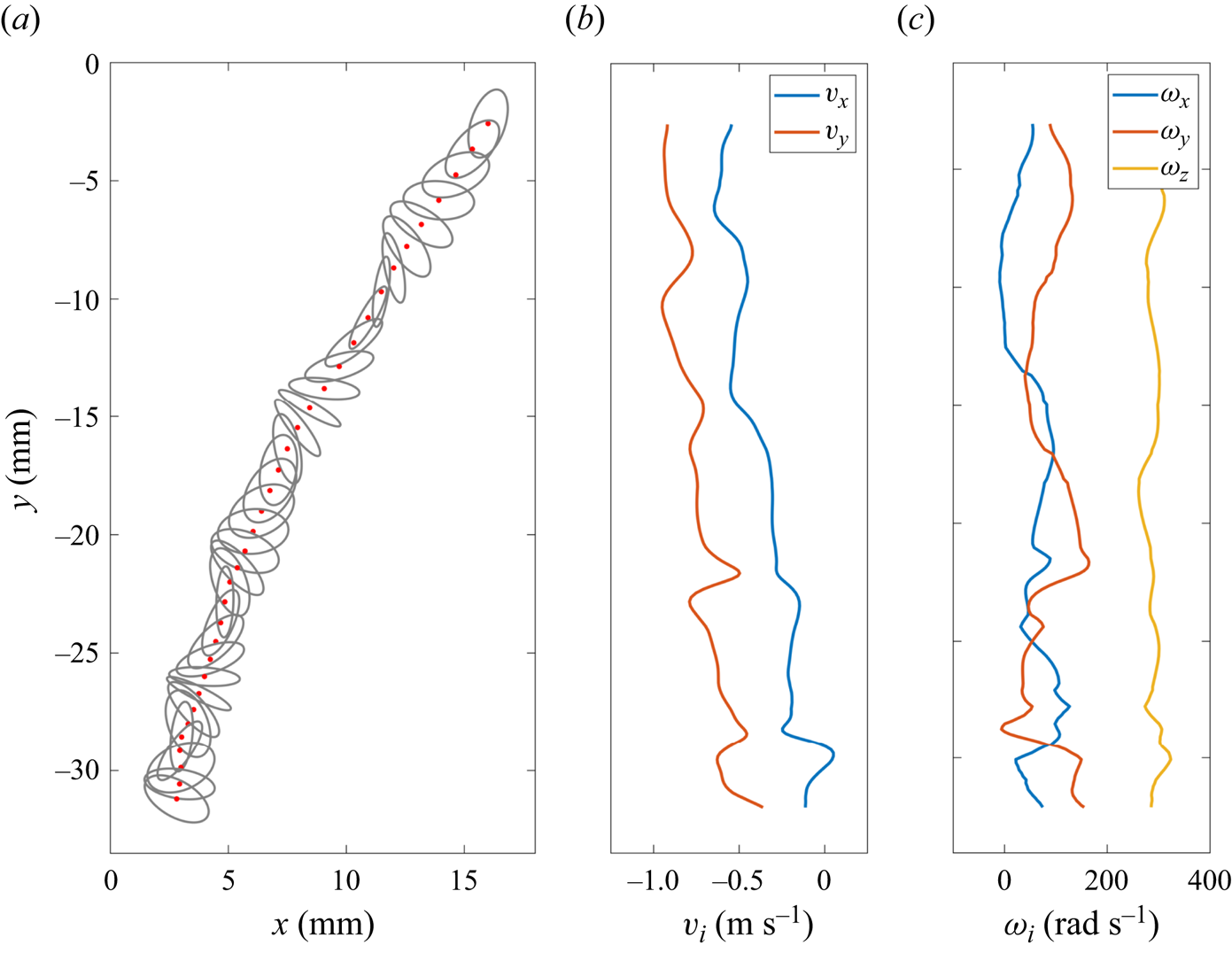
An example trajectory of a 3 mm disk in stronger turbulence is provided in figure 3 with this processing method applied. As will be discussed in § 3, this trajectory demonstrates the typical influence of turbulence that we observe on the disks: the vertical velocity is reduced as the disk is forced laterally, while the angular velocity is sustained at a constant rate.
Sample processing result of a 3 mm disk in stronger turbulence. (a) Ellipse fits to disk image shown in grey every 5 frames (every  $1.16 \times 10^{-3}$ s), with centroids marked in red. Values shown along the trajectory include (b) horizontal velocity $v_x$ and vertical velocity $v_y$, and (c) three-dimensional angular velocity components.
Statistics are obtained from  $O(10^3\unicode{x2013}10^4)$ trajectories for each case, with typical trajectory lengths of $O(10^2)$ frames. Even in the SFV, the relative resolution of the 0.3 and 0.5 mm disks is lower than for the larger disks, and their orientation is not accurately reconstructed. Therefore, we will report on their translational motion and comment qualitatively only on their orientation and rotation.
3. Results
3.1. Parameter space for disks falling in turbulence
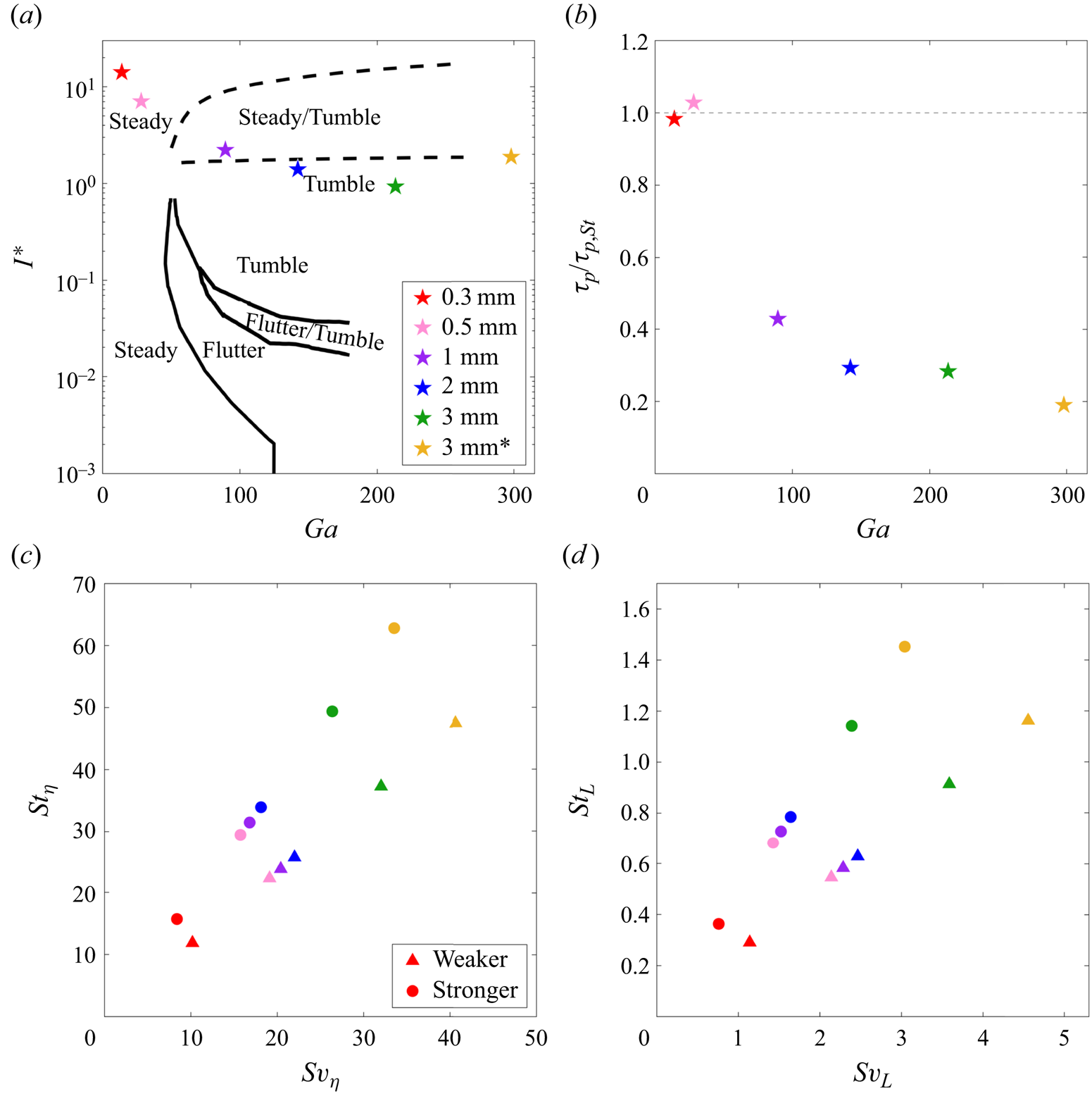
We begin by placing the investigated cases in the appropriate non-dimensional parameter spaces. Figure 4(a) displays the  $I^*$– $Ga$ plane, often adopted to describe the disk falling style in otherwise quiescent fluids. This shows that the sub-millimetre disks are expected to fall steadily, while those with $D \geq 1$ mm land along the transition region to the tumbling regime. We will see how this prediction compares with our observations in still air, and how turbulence affects it.
(a) Quiescent falling style parameter space plotted as inertia ratio  $I^*$ versus Galileo number $Ga$. Falling mode boundaries identified by Auguste et al. (Reference Auguste, Magnaudet and Fabre2013) shown with solid black lines, and bounding limits of region of bistability found by Lau et al. (Reference Lau, Huang and Xu2018) indicated by dashed black lines. Data from those publications was digitized using WebPlotDigitizer (Rohatgi Reference Rohatgi2021). (b) Empirically determined particle response time $\tau _p$ based on the measured settling velocity normalized by the particle response time based on a Stokesian flow assumption $\tau _{p,St}$ defined by Gustavsson et al. (Reference Gustavsson, Sheikh, Naso, Pumir and Mehlig2021), plotted versus Galileo number. (c) Stokes number $St_{\eta }$ versus settling velocity number $Sv_{\eta }$ based on the Kolmogorov scale of the turbulence. (d) Stokes number $St_L$ versus settling velocity number $Sv_L$ based on the integral scale of the turbulence.
The particle's ability to follow turbulent fluctuations is commonly characterized by the aerodynamic response time  $\tau _p$. For small $Re$, Stokesian drag formulations apply, and $\tau _p$ can be obtained analytically: for ellipsoids with semi-axes $a_{\parallel }=h/2$ and $a_{\perp }=D/2$, the Stokesian response time is $\tau _{p,St}=(2 a_{\parallel } a_{\perp } \rho _p)/(9 \nu \rho _f)$ (Gustavsson et al. Reference Gustavsson, Sheikh, Lopez, Naso, Pumir and Mehlig2019, Reference Gustavsson, Sheikh, Naso, Pumir and Mehlig2021). For the present range of $Re$, the actual response time is estimated by measuring the terminal velocity in still air and applying a balance between drag and gravity, $\tau _p = V_{t,0}/g$. Figure 4(b) plots $\tau _p/\tau _{p,St}$ versus $Ga$, and shows how the Stokesian estimate is still tenable for the 0.3 and 0.5 mm disks, even though $Re = O(10)$. The dramatic drop in response time for $D \geq 1$ mm signals the inertial contribution to the drag becoming dominant.
Sheikh et al. (Reference Sheikh, Gustavsson, Lopez, Lévêque, Mehlig, Pumir and Naso2020) showed by theoretical considerations that the relative importance of inertial versus viscous torque for falling ellipsoids is given by the parameter  $\mathcal {R} \equiv |\boldsymbol {u} - \boldsymbol {v}|^2 /[\nu \,|\boldsymbol {\varOmega } - \boldsymbol {\omega }|]$, where $\boldsymbol {v}$ and $\boldsymbol {u}$ are the particle and fluid velocities, respectively, $\boldsymbol {\varOmega }$ is half the vorticity, and $\boldsymbol {\omega }$ is the particle angular velocity. As we do not measure the fluid velocity and vorticity around the disks, we estimate $\mathcal {R} = ({V_t}/{u'})^2\,Re_L^{1/2} \sim Sv_{\eta }^2$, where $Re_L = u'L/\nu$ (Anand et al. Reference Anand, Ray and Subramanian2020; Sheikh et al. Reference Sheikh, Gustavsson, Lopez, Lévêque, Mehlig, Pumir and Naso2020). The theory assumes Stokesian drag, thus it holds to first order for the sub-millimetre disk. Even for our smallest disk, $D=0.3$ mm, under different turbulence levels, $\mathcal {R} = 46.2\unicode{x2013}73.5 \gg 1$, thus predicting a dominant role of inertial torque. At higher $Re$, the relative contribution of the viscous torque is expected to be even smaller. Therefore, we expect the disks to preferentially adopt a broad-side-first orientation (Anand et al. Reference Anand, Ray and Subramanian2020; Sheikh et al. Reference Sheikh, Gustavsson, Lopez, Lévêque, Mehlig, Pumir and Naso2020), as opposed to falling edge-first and minimizing drag (which is instead seen in simulations that assume a torque formulation linear in the velocity; see Gustavsson et al. Reference Gustavsson, Jucha, Naso, Lévêque, Pumir and Mehlig2017; Jucha et al. Reference Jucha, Naso, Lévêque and Pumir2018). This expectation will be verified in § 3.2.
The estimate of  $\tau _p$ allows us to evaluate the Stokes number $St$, which is plotted versus the settling parameter $Sv$ using Kolmogorov scales (figure 4c) and integral scales (figure 4d). This representation has been used to describe the particle–turbulence interaction and gravitational settling of small spherical particles (Good et al. Reference Good, Ireland, Bewley, Bodenschatz, Collins and Warhaft2014; Rosa et al. Reference Rosa, Parishani, Ayala and Wang2016; Petersen et al. Reference Petersen, Baker and Coletti2019). It highlights how all considered disks possess significant inertia compared to the Kolmogorov scales, while their response time and still-air fall speed are comparable to the integral scales of the turbulence.
The  $St\unicode{x2013}Sv$ parameter space has also been used for non-spherical particles in turbulence by Gustavsson et al. (Reference Gustavsson, Sheikh, Naso, Pumir and Mehlig2021), who assumed negligible inertial drag to derive a regime map for the orientation variance. As just shown, their assumption is tenable only for the sub-millimetre disks. Even those have $St_{\eta } \gg 1$ and $Sv_{\eta } \gg 1$, and according to Gustavsson et al. (Reference Gustavsson, Sheikh, Naso, Pumir and Mehlig2021), they land in a regime where both translational and rotational dynamics are underdamped. Their model yields specific predictions on the typical tilting angles, which we unfortunately cannot verify due to the above-mentioned limitations in reconstructing the small disk orientation. However, as we will discuss in § 3.3, our observations are at least in qualitative agreement with their theory.
3.2. Translational motion
The normalized and centred distributions of instantaneous vertical disk velocity fluctuations are shown in figure 5 for the 0.3 and 2 mm disks, which are representative of the cases with  $D < 1$ mm and $D \geq 1$ mm, respectively. Here and in the following, $V_t = \langle -v_y \rangle$, where $-v_y$ is the downward instantaneous vertical velocity of the disks, and angle brackets indicate ensemble averaging. The spread in the distributions is largely due to the trajectory-to-trajectory variability, which is more than 10 times larger than the variability within a given trajectory. This confirms that the disks mostly respond to the large-scale turbulent fluctuations, as anticipated by the ranges of $St$ and $Sv$ in figure 4. The probability density functions (PDFs) of the vertical velocity fluctuations for the sub-millimetre disks are nearly symmetric and Gaussian for all flow conditions (figure 5a), while those for $D \geq 1$ mm are visibly skewed towards larger downwards velocities (figure 5b). Distributions of horizontal velocities (not shown) are approximately Gaussian independently of the ambient turbulence.
The PDFs of instantaneous vertical velocity, normalized and centred using the r.m.s.  $v_y'$ for comparison of all curves to a Gaussian distribution: (a) 0.3 mm disks, and (b) 2 mm disks.
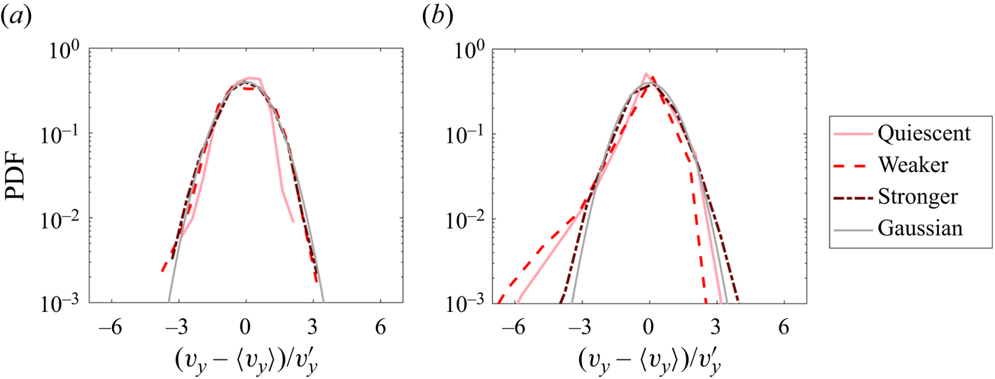
The skewness of the vertical velocity fluctuations in quiescent conditions is attributed to fluid entrainment in the unsteady wake, intermittently accelerating the disk's descent (Tinklenberg et al. Reference Tinklenberg, Guala and Coletti2023), similarly to what has been observed for rising bubbles in similar ranges of  $Re$ (Risso Reference Risso2018). This behaviour emerges for $Re \gtrsim 100$, for which the transition to an unsteady wake is expected (Willmarth et al. Reference Willmarth, Hawk and Harvey1964; List & Schemenauer Reference List and Schemenauer1971). The skewness survives in the weaker turbulence but is extinguished by the stronger turbulence, in which an approximately Gaussian distribution is recovered. This is interpreted as the consequence of the turbulence disrupting the wakes, as reported in numerical studies for spherical particles (Bagchi & Balachandar Reference Bagchi and Balachandar2003; Fornari et al. Reference Fornari, Picano and Brandt2016a) and bubbles (Merle, Legendre & Magnaudet Reference Merle, Legendre and Magnaudet2005).
Figure 6(a) reports the mean settling velocity, which is found to be reduced by the turbulence for all considered types of disks, with a decrease of up to 35 % for the 3 mm disks in the stronger turbulence. Here and in the following, error bars are calculated from the statistical uncertainty  $\sigma /\sqrt {N}$, where $\sigma$ is the standard deviation over the data set, and $N$ is the number of experimental runs. This conservatively assumes that all trajectories in each run are statistically correlated.
(a) Mean disk terminal velocity  $V_t$ plotted as function of disk type for each flow condition. (b) Reynolds number calculated from $V_t$ in (a) as $Re=V_t D/\nu$, plotted against Galileo number $Ga$.
$Ga$.
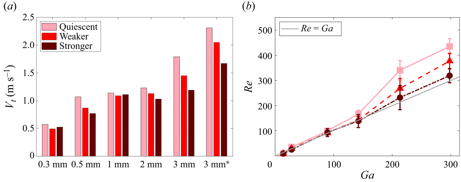
Non-dimensionalizing the results as  $Re$ versus $Ga$ (figure 6b) highlights an important trend. In quiescent air, the larger and heavier disks increasingly depart from the line marking $Re = Ga$, which corresponds to a nominal drag coefficient $C_D = 1$.
As is customary for free-falling bodies in general and frozen hydrometeors in particular (Böhm Reference Böhm1989; Heymsfield & Westbrook Reference Heymsfield and Westbrook2010), we evaluate  $C_D$ through the drag–gravity balance in the vertical direction:
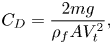 \begin{equation} C_D = \frac{2mg}{\rho_f A V_t^2}, \end{equation}
where  $m$ is the object mass, and $A$ is its projected area normal to the falling motion. We take the latter as the disk frontal area ${\rm \pi} D^2/4$, which is consistent with previous studies (e.g. Willmarth et al. Reference Willmarth, Hawk and Harvey1964) and with the prevalent horizontal alignment anticipated above and demonstrated in the following. The drag coefficient is plotted versus $Re$ in figure 7 for both quiescent and turbulent air, and compared to previous experiments where disks fall in quiescent liquids (hence $\tilde {\rho } < 10$, from 1.03 in McCorquodale & Westbrook (Reference McCorquodale and Westbrook2021a) to 9.5 in Jayaweera (Reference Jayaweera1965)). Those deviate significantly from the present results. This is a consequence of the much higher density ratio in air, which implies higher translational and rotational inertia (quantified parametrically by $St$ and $I^*$, respectively). This profoundly alters the coupling between the object motion and its wake compared to the case $\tilde {\rho } = O(1)$, resulting in large downward accelerations during phases of the motion in which the disks fall edge-on (Tinklenberg et al. Reference Tinklenberg, Guala and Coletti2023).
(a) Drag coefficient  $C_D$ versus Reynolds number $Re$ plotted over data from Willmarth et al. (Reference Willmarth, Hawk and Harvey1964), Jayaweera (Reference Jayaweera1965), Jayaweera & Cottis (Reference Jayaweera and Cottis1969) and McCorquodale & Westbrook (Reference McCorquodale and Westbrook2021a) in grey symbols. Correlation for spheres in quiescent fluid shown in black line (Roos & Willmarth Reference Roos and Willmarth1971; Brown & Lawler Reference Brown and Lawler2003). (b) Zoom-in on the region of interest in the present study.
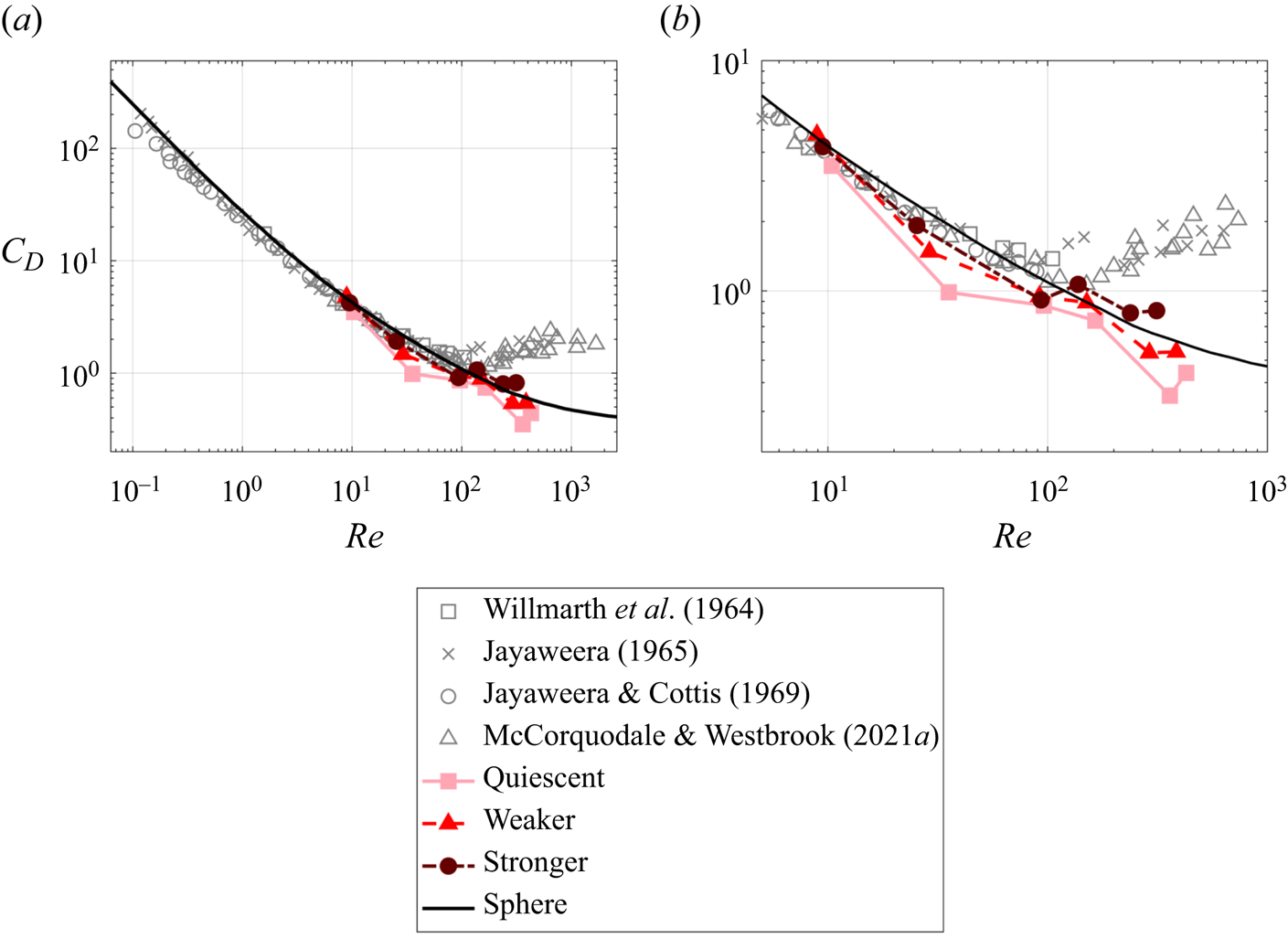
The addition of ambient turbulence progressively reduces  $V_t$, which implies lower $Re$ for a given $Ga$ (figure 6b), and higher $C_D$ for a given $Re$ (figure 7). To understand this result, we consider the definition of the drag coefficient:
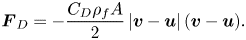 \begin{equation} \boldsymbol{F}_D =-\frac{C_D \rho_f A}{2}\,|\boldsymbol{v}-\boldsymbol{u}|\,(\boldsymbol{v}-\boldsymbol{u}). \end{equation}
In the linear drag regime,  $C_D \sim 1/Re \sim 1/|\boldsymbol {v}-\boldsymbol {u}|$; hence the linear drag relation $\boldsymbol {F}_D \sim (\boldsymbol {u}-\boldsymbol {v})$. This implies that in a zero-mean flow, the effects of turbulent velocity fluctuations are averaged out and do not alter the mean drag force acting on the settling particle. In the present regime, on the other hand, $Re = O(10^1\unicode{x2013}10^2)$ and $C_D$ has a weaker dependence on $Re$, thus the drag force grows more than linearly with the slip velocity. The increase of the latter caused by the turbulent fluctuations thus yields a net increase of the drag force, which is prevalently directed upwards (Tunstall & Houghton Reference Tunstall and Houghton1968; Fornari et al. Reference Fornari, Picano, Sardina and Brandt2016b). The resulting reduction of mean settling velocity was discussed in detail by, among others, Fornari et al. (Reference Fornari, Picano, Sardina and Brandt2016b). These authors performed PR-DNS on spherical particles falling in homogeneous turbulence, and analysed the influence of the fluid velocity fluctuations on the mean drag using finite- $Re$ corrections. They distinguished between the contributions due to the vertical and horizontal fluctuations, termed nonlinear-induced drag and cross-flow-induced drag, respectively. It should be noted, however, that both effects are rooted in the nonlinearity of the drag with the slip velocity.
Though we do not measure the local fluid velocity around the disks, we can infer the importance of the nonlinear-induced and cross-flow-induced drag by considering the turbulence properties and the disk trajectories. The nonlinear-induced drag is expected to be significant when the instantaneous vertical slip velocity is sizeably affected by the turbulent fluctuations. This is clearly the case here:  $u'$ is comparable to $V_t$, especially in the stronger turbulence for which $Sv_L = 0.8\unicode{x2013}3$ (see figure 4d).
The cross-flow-induced drag, on the other hand, is associated with lateral sweeps experienced by the particles falling through turbulent gusts, which impart significant lateral velocity on them. This is signalled by the angle  $\phi$ between the vertical direction and the disk trajectories projected along the imaging plane, which are well approximated by straight lines in our limited field of view (coefficient $R^2 > 0.9$; figure 8a). Figure 8(b) shows that the representative 1 mm disks barely reach $\phi \sim 15^{\circ }$ when tumbling in still air, due to the rotation-induced lift (Belmonte, Eisenberg & Moses Reference Belmonte, Eisenberg and Moses1998; Fabre, Assemat & Magnaudet Reference Fabre, Assemat and Magnaudet2011; Tinklenberg et al. Reference Tinklenberg, Guala and Coletti2023). On the other hand, $\phi$ can be as large as $35^{\circ }$ and $75^{\circ }$ in the weaker and stronger turbulence, respectively. For all considered cases, the r.m.s. lateral velocity of the disks, $v_x'$ (expected to be of order $V_t \langle \tan |\phi | \rangle$) is found to be smaller than, but comparable to, the characteristic magnitude of the horizontal fluid fluctuations, $u_x'$. This is consistent with the notion that the disk lateral motions are driven mostly by the cross-flow effect. More importantly, we find that the cross-flow-induced tilting of the trajectories correlates with settling reduction, as predicted by the nonlinear drag framework. This is shown clearly by the vertical velocity PDF of the 1 mm disks in the stronger turbulence, conditioned on the values of $\phi$ (figure 8c), with large trajectory angles corresponding to significantly smaller fall speeds. Figure 8(d) summarizes the effect of the turbulence on the trajectory inclination for all cases. The increase in $\phi$ is the largest for the sub-millimetre disks, due to their smaller inertia. However, as discussed in § 3.1, their translational dynamics are only weakly nonlinear. Indeed, the fall speed of the smallest disks is marginally affected by the turbulence (see figure 6).
(a) Centroid trajectories of 1 mm disks in stronger turbulence demonstrating the wide range of  $\phi$ induced by the turbulence. (b) Distributions of trajectory angle modulus $|\phi |$ for 1 mm disks in quiescent air, weaker turbulence and stronger turbulence. (c) Instantaneous vertical velocity of the 1 mm disks in stronger turbulence, binned by ranges of trajectory angle. (d) Mean $|\phi |$ values in each flow condition for all disk types, labelled by $Ga$.
$Ga$.
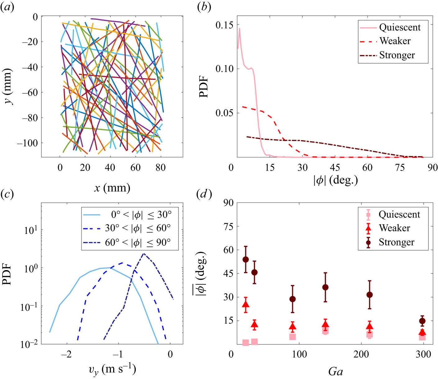
As discussed by Fornari et al. (Reference Fornari, Picano and Brandt2016a,Reference Fornari, Picano, Sardina and Brandtb), ambient turbulence can also affect the mean settling velocity of heavy particles by changing the magnitude of the unsteady forces such as added mass, stress gradient and Basset history force. Ling, Parmar & Balachandar (Reference Ling, Parmar and Balachandar2013) derived general scaling relations for such forces, and found their magnitude relative to the drag to be at most  ${\sim }St_{\eta }/(\tilde {\rho } -1)$. As this amounts to just a few per cent in the present cases, we deem their effect negligible, at least regarding the mean settling rate. For rotating non-spherical particles, the lift force is also expected to be significant and unsteady in nature. Its role will be discussed in § 3.3.
In the above, we have not considered the possibility that the disks may sample the turbulent velocity field non-uniformly. In fact, as mentioned in § 1, the settling velocity of particles in turbulence may also be affected by the preferential sampling of upward or downward fluid velocity fluctuations, referred to as loitering and preferential sweeping, respectively. Both such effects require that the particles be able to respond to the turbulent fluctuations over relevant time scales. This responsiveness can be estimated by comparing  $\tau _p$ with the settling time scale $\tau _s$, i.e. the time needed for a falling particle to cross the turbulence correlation length scale. Following Gustavsson et al. (Reference Gustavsson, Sheikh, Naso, Pumir and Mehlig2021), we take the latter as the Taylor microscale $\lambda$, i.e. the scale over which the velocity gradients are correlated, $\tau _s = \lambda /V_{t,0}$. Noting that $\lambda \sim u' \tau _{\eta }$, we have $\tau _p/\tau _s \sim St_{\eta }\, Sv_L$. Petersen et al. (Reference Petersen, Baker and Coletti2019) indeed noted that the normalized fall speed $V_t/V_{t,0}$ of spherical particles in turbulence collapsed when plotted against the group $St_{\eta }\,Sv_L$, with preferential sweeping confined to $St_{\eta }\,Sv_L = O(10^{-1})$. In the present case, $St_{\eta }\,Sv_L = O(10^1\unicode{x2013}10^2)$, suggesting that the falling disks are not sufficiently responsive to the turbulence to achieve preferential sweeping. Loitering, on the other hand, cannot be excluded a priori (though previous studies on spherical particles at similar $Re$ found no evidence of it; Fornari et al. Reference Fornari, Picano, Sardina and Brandt2016b). To clarify this point, simultaneous measurements of the disk motion and turbulent flow would be needed.
3.3. Rotational dynamics
While the imaging of sub-millimetre disks does not possess sufficient resolution to accurately reconstruct their orientation, inspection of the recordings for the 0.3 mm disks indicates that these fall steadily in both quiescent and turbulent air. Examples are reported in figures 9(a,b). In quiescent air, this observation is consistent with their position in the  $I^*\unicode{x2013}Ga$ parameter space (see figure 4a). In turbulent air, the approximately steady falling is consistent with the theory of Gustavsson et al. (Reference Gustavsson, Sheikh, Naso, Pumir and Mehlig2021): their mapping of the orientation variance in the $St_{\eta }\unicode{x2013}Sv_{\eta }$ space predicts that disks with $D = O(0.1\ {\rm mm})$ would oscillate between tilting angles of a few degrees from the horizontal. The 0.5 mm disks also appear to fall steadily in still air (figure 9c), while they often flutter in turbulent air (figure 9d). However, the crucial result of the theory by Gustavsson et al. (Reference Gustavsson, Sheikh, Naso, Pumir and Mehlig2021) is the dependence of the orientation variance with $Sv_{\eta }$, which unfortunately we cannot verify quantitatively because of the limited resolution.
Disk image progressions shown in quiescent air and stronger turbulence, respectively, for (a,b) a 0.3 mm disk, and (c,d) a 0.5 mm disk. All progressions shown every fourth frame capture of the original disk images (every  $9.3 \times 10^{-4}$ s). Supplementary movies are available at https://doi.org/10.1017/jfm.2024.534.
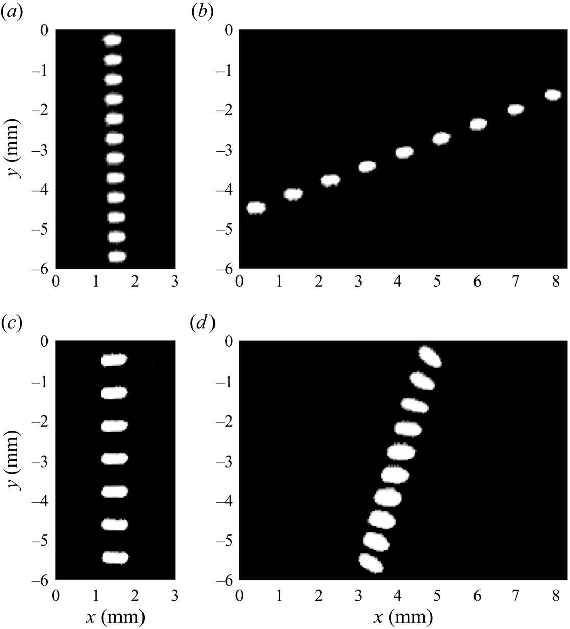
We now analyse the disk orientation and rotation rate for  $D \geq 1$ mm. Figure 10 shows PDFs of the vertical component of $\hat {\boldsymbol {p}}$ for the representative cases $D = 1$ and 3 mm. In both cases, and especially for $D = 3$ mm, the broadside-on orientation ( $|p_y| \sim 1$) is prevalent in quiescent air, while the edge-on orientation ( $|p_y| \sim 0$) is the least likely. This trend is visible also in turbulent air, and verifies the expectation based on the parameter $\mathcal {R}$ as discussed in § 3.1. Stronger turbulence, however, produces increasingly flatter distributions. This intuitive trend is consistent with the numerical and theoretical findings of Anand et al. (Reference Anand, Ray and Subramanian2020). Their model too, however, assumed Stokesian drag, therefore any comparison can be only qualitative. We note, in particular, that the observed randomization of the orientation is much more pronounced than in their simulations: in the stronger turbulence, the broadside-on orientation is only approximately three times more frequent than the edge-on orientation. This behaviour is also likely to magnify the effect of the lateral cross-flow, as more tilted disks offer a larger effective area to the horizontal turbulent fluctuations.
The PDFs of the modulus of the instantaneous disk orientation vector with respect to the vertical ( $y$) for (a) 1 mm disks, and (b) 3 mm disks.

The above indicates that ambient turbulence alters the disk falling style, shifting it away from steady falling and increasingly towards tumbling. This is visible from the recordings and confirmed by analysing the change in orientation along each trajectory. In figure 11, we plot, again for  $D = 1$ and 3 mm, the angular excursion $\Delta p_y$, i.e. the range of $p_y$ values spanned by a disk during its trajectory. This allows us to distinguish between steady falling, fluttering and tumbling, which we conventionally associate to the ranges $0 \leq \Delta p_y < 0.5$, $0.5 \leq \Delta p_y < 1.5$ and $1.5 \leq \Delta p_y \leq 2$, respectively (Tinklenberg et al. Reference Tinklenberg, Guala and Coletti2023). The labelling is nominal, and the exact definitions do not alter the conclusions. In quiescent air, the distributions are bimodal for both considered disk sizes, with a prevalence of either tumbling ( $D = 1$ mm) or steady falling ( $D = 3$ mm). With increasing turbulence, the fraction of steady falling trajectories is generally reduced, increasing the occurrence of tumbling and fluttering (the latter being virtually absent in still air). Interestingly, the distributions of angular excursion are similar for both disks in strong turbulence, though they are markedly different in still air.
(a–c) Histograms of  $\Delta p_y$ shown for the 1 mm disks in quiescent air, weaker turbulence and stronger turbulence, respectively. (d–f) Similarly for the 3 mm disks. Shading indicates falling style regions: $0 \leq \Delta p_y < 0.5$ is steady flat-falling, $0.5 \leq \Delta p_y < 1.5$ indicates a fluttering disk, and $1.5 \leq \Delta p_y \leq 2$ represents disks tumbling.
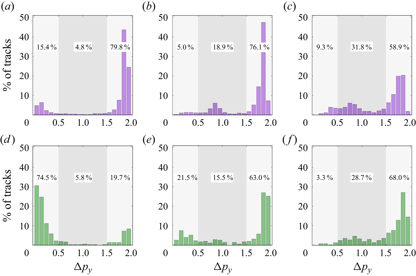
The shift away from steady falling caused by ambient turbulence also affects the disk angular velocity  $\boldsymbol {\omega }_t=\hat {\boldsymbol {p}} \times \dot {\hat {\boldsymbol {p}}}$. As we do not capture spinning, we refer interchangeably to rotation rate and tumbling rate. Distributions of the magnitude $|\omega _t|$, averaged along each trajectory and plotted in figure 12, illustrate the trends with varying turbulence intensity and disk properties. In still air (figure 12a), the bimodal PDFs reflect that seen above for the angular excursion. Visual observation confirms that trajectories with $|\omega _t|$ larger and smaller than approximately 100 rad s $^{-1}$ are characterized by steady falling and tumbling, respectively. All disks for which we track the orientations exhibit a bimodal behaviour in still air (both non-tumbling and tumbling modes occurring with significant probabilities), except for the 2 mm disks, which invariably tumble. As the values of $I^*$ are relatively close for all cases, we hypothesize that the particular behaviour of the 2 mm disk depends on its Galileo number, $Ga = 142$. This is in the range where oblate particles have been reported to exhibit subtle changes of falling style, though these have been mapped in detail only for much lower density ratios (Chrust et al. Reference Chrust, Bouchet and Dušek2013; Moriche et al. Reference Moriche, Uhlmann and Dušek2021).
The PDFs of trajectory-averaged angular velocity magnitude plotted for disks with  $D \geq 1$ mm in (a) quiescent air, (b) weaker turbulence, and (c) stronger turbulence.
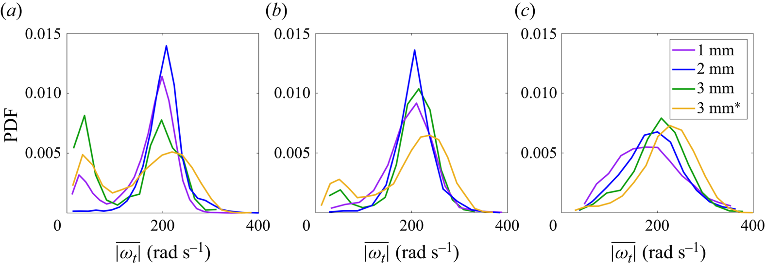
Introducing and increasing ambient turbulence (figures 12b,c) reduces and eventually obliterates the bimodal behaviour, preventing the steady falling style. Especially in strong turbulence, the angular velocity distributions are centred around peak values  $\omega _{peak}$ that increase with disk diameter and thickness, i.e. with fall speed. This is consistent with the notion that the rotation is dominated by inertial torque: unlike its Stokesian counterpart, this is directly dependent on the slip velocity, which to first order scales as the fall speed (Sheikh et al. Reference Sheikh, Gustavsson, Lopez, Lévêque, Mehlig, Pumir and Naso2020). Moreover, for the same disk type, $\omega _{peak}$ is altered only moderately by the turbulence. This demonstrates that in the present parameter range, the tumbling rate is predominantly set by the disk rotational inertia rather than by the fluid inertia.
The above trends for the angular velocity have been shown by using dimensional units. Appropriate non-dimensionalization of this quantity is not trivial, as it requires identifying the characteristic time scale of rotation. Theoretical estimates are available only in the Stokesian drag limit, outside of which it is usually determined experimentally (Kramel Reference Kramel2017; Gustavsson et al. Reference Gustavsson, Sheikh, Naso, Pumir and Mehlig2021; Roy et al. Reference Roy, Kramel, Menon, Voth and Koch2023). In Tinklenberg et al. (Reference Tinklenberg, Guala and Coletti2023), we proposed that the rotation time scale of inertial disks in quiescent air be set by the response time  $\tau _p$, independent of the surrounding flow. This is consistent with the observation that turbulence has a limited effect on $\omega _{peak}$.
The alternative non-dimensionalization consists in defining the Strouhal number  $Str = fD/V_t$, where $f$ is the characteristic frequency of the oscillatory motion (Ern et al. Reference Ern, Risso, Fabre and Magnaudet2012). Here, $Str$ is proportional to the tip speed ratio $\omega _t (D/2)/V_t$ of the tumbling disk and represents a measure of the rotational velocity over the translational velocity of the disk. As is customary (e.g. Chrust et al. Reference Chrust, Bouchet and Dušek2013; Esteban et al. Reference Esteban, Shrimpton and Ganapathisubramani2020), we take $f$ as the characteristic frequency of the velocity signal, i.e. twice the frequency of the full tumbling motion, $f = 2f_{peak}= \omega _{peak}/{\rm \pi}$. Plotting $Str$ as function of $Ga$, there appears to be a peak for $Ga = 213$ (figure 13a). However, this may be a consequence of how the data points are distributed on the $I^*\unicode{x2013}Ga$ parameter space; i.e. the behaviour is likely driven by the decrease of $Str$ with $I^*$ shown in figure 13(b). The values of $Str$ and its decreasing trend with $I^*$ are indeed consistent with previous studies of tumbling disks (Willmarth et al. Reference Willmarth, Hawk and Harvey1964; Auguste et al. Reference Auguste, Magnaudet and Fabre2013). While the range is too small to verify a scaling law, our results are compatible with the relation $Str \sim {I^*}^{-0.5}$ proposed by Fernandes et al. (Reference Fernandes, Risso, Ern and Magnaudet2007).
Strouhal number  $Str = fD/V_t$ plotted as function of (a) $Ga$ and (b) $I^*$.

Turbulence does not change this trend qualitatively. Esteban et al. (Reference Esteban, Shrimpton and Ganapathisubramani2020) also found that turbulence did not substantially change the dominant oscillation frequency of their disks falling in water. In their case, however, the effect of turbulence on the frequency distributions was fundamentally different from what we observe. They found that a relatively slow, turbulence-induced frequency appeared, and attributed it to a long gliding phase triggered by eddies perturbing the disks at the inversion point of fluttering trajectories. Their disks were in a range of the settling velocity parameter similar to ours ( $Sv_L = 1.5\unicode{x2013}7$) but had much weaker rotational inertia relative to the fluid ( $I^* = O(10^{-3})$, three orders of magnitude smaller than here), thus were much more prone to be disturbed by the ambient fluctuations. In the present case, the turbulent eddies can influence the rotational dynamics by destabilizing the steady-falling disks and causing them to start tumbling; but then the disk inertia is too large for the eddies to modify their rotation rate.
As tumbling is the dominant falling style in turbulent air, rotation-induced lift could be expected to play a role in the dynamics. In quiescent air, as mentioned, the tumbling disks indeed drift in direction  $\boldsymbol {\omega }_t \times \boldsymbol {u}_p$ (Belmonte et al. Reference Belmonte, Eisenberg and Moses1998; Andersen, Pesavento & Wang Reference Andersen, Pesavento and Wang2005; Tinklenberg et al. Reference Tinklenberg, Guala and Coletti2023), and the lift force can be estimated as $F_L \sim F_D \tan (\phi )$, i.e. up to 20 % of the drag. In turbulent air, although the rotation rate of the tumbling disk is not dramatically altered, we find no correlation between the sense of rotation and the direction or magnitude of the disk lateral velocity. The latter is in fact largely driven by the turbulent gusts, as discussed in § 3.1. Thus while rotation-induced lift is likely present, its effect is difficult to discern because ambient turbulence alters the coupling between translational and rotational motion.
4. Conclusion
We have investigated experimentally the influence of turbulence on the settling of thin solid disks in air. Using a laboratory apparatus featuring hundreds of randomly actuated jets, we have generated two levels of homogeneous turbulence, with velocity fluctuations smaller than but comparable to the disk settling velocities. Within the limits of a laboratory study, the properties of the system (and so the range spanned by the main non-dimensional parameters) are relevant to precipitating plate crystals in the atmosphere. Using laser illumination and high-speed imaging, we have gathered and analysed the objects’ translational and rotational dynamics based on thousands of trajectories.
The smaller disks that we have considered (0.3 and 0.5 mm in diameter) tend to fall broadside-on and at a speed close to the Stokesian prediction, independently of the ambient turbulence. This agrees with recent theoretical and numerical studies in which the inertial drag was neglected but the inertial torque was considered (Anand et al. Reference Anand, Ray and Subramanian2020; Sheikh et al. Reference Sheikh, Gustavsson, Lopez, Lévêque, Mehlig, Pumir and Naso2020). On the other hand, the motion of the larger disks (1–3 mm in diameter) is strongly affected by the turbulence in two important aspects.
First, the fall speed is decreased, this effect being stronger with increasing turbulence intensity and disk size. For the 3 mm disks in the stronger turbulence, the reduction in mean vertical velocity amounts to approximately 35 % of the still-air terminal velocity. This is attributed to nonlinear drag effects: the turbulent fluctuations in both vertical and horizontal directions increase the slip velocity magnitude between the disks and the surrounding fluid, causing a net augmentation of the drag force and thus retarding their descent. In particular, the cross-flow-induced drag is demonstrated most clearly by the systematically slower settling of disks with strong lateral motions. The decrease of the settling rate due to nonlinear drag has been documented for spherical particles, for which classic empirical correlations have been used to account for finite  $Re$ (Clift, Grace & Weber Reference Clift, Grace and Weber2005). For example, Homann et al. (Reference Homann, Bec and Grauer2013) proposed a model that utilizes the Schiller & Naumann (Reference Schiller and Naumann1933) correlation and was shown to predict reasonably well the settling reduction of finite-size spheres in turbulence (Chouippe & Uhlmann Reference Chouippe and Uhlmann2019). For highly anisotropic particles, expressions that take shape into account (e.g. Bagheri & Bonadonna Reference Bagheri and Bonadonna2016) may inform future models able to capture the present results. Besides nonlinear drag, the influence of preferential sweeping and unsteady effects on the mean fall speed are deemed negligible based on scaling arguments, although the former may become significant for much smaller disks approaching $St_{\eta }\,Sv_L \sim O(0.1)$. Further studies including the simultaneous measurements of both disk and fluid velocity are needed to ascertain the possible role of loitering.
Second, ambient turbulence causes the millimetre-sized disks to tumble systematically, while in still air they exhibit a bimodal behaviour in which steady falling and tumbling coexist. As a result, while the broadside-on position is still prevalent, the orientation distribution is much more randomized than in quiescent ambient. Even the stronger forcing, however, does not significantly alter the dominant rotation rates: in other words, ambient turbulence can trigger the tumbling motion, but not drive it to a specific frequency. Indeed, the Strouhal number based on the rotational frequency has a similar dependence on the inertia ratio  $I^*$ regardless of the turbulence intensity, consistent with the results from Willmarth et al. (Reference Willmarth, Hawk and Harvey1964).
It is interesting to compare the present findings against the only two previous experimental studies that investigated disks falling in turbulence, Byron et al. (Reference Byron, Einarsson, Gustavsson, Voth, Mehlig and Variano2015) and Esteban et al. (Reference Esteban, Shrimpton and Ganapathisubramani2020), while keeping in mind their different place in the parameter space (see table 1). Byron et al. (Reference Byron, Einarsson, Gustavsson, Voth, Mehlig and Variano2015) found that turbulence reduced the settling velocity of their weakly oblate particles in water by up to 40 %. This was not related to the particle shape, as prolate particles of similar volume behaved analogously. According to the analysis of Fornari et al. (Reference Fornari, Picano and Brandt2016a,Reference Fornari, Picano, Sardina and Brandtb), the reduced settling speed was due to a combination of nonlinear drag and unsteady effects, the latter playing a larger role. Those are expected to be large for such particles that were marginally heavier than water, while they are negligible in the present case. The nonlinear drag effect, on the other hand, is likely stronger for our disks even if  $Re$ is comparable, due to the much larger aspect ratio $\chi$: the highly non-spherical shape promotes the separation of the flow around them, which in turn is the root of the drag nonlinearity (Clift et al. Reference Clift, Grace and Weber2005). Conversely, Esteban et al. (Reference Esteban, Shrimpton and Ganapathisubramani2020) found that turbulence enhanced the settling of thin disks in water. They attributed this to edge-on gliding phases in the fluttering trajectories, induced by the perturbing action of eddies of size comparable to the disks. Fluttering was indeed the dominant falling style in their study, due to the relatively high $Ga$ and low $I^*$. Our disks, on the other hand, are predominantly in the steady falling or tumbling state. More importantly, as discussed, air turbulence can destabilize otherwise steadily falling disks, but the fluid inertia is not sufficient to alter the tumbling rate. Therefore, the mechanism observed by Esteban et al. (Reference Esteban, Shrimpton and Ganapathisubramani2020) is not in play. This comparative analysis demonstrates the complexity of the problem of non-spherical particles falling in turbulence, which is governed by multiple important parameters whose influence is best understood when varying them one at a time. In particular, further research is warranted to systematically explore the role of the density ratio.
The present study is the first to tackle experimentally a regime fully relevant to plate crystals precipitating in atmospheric turbulence, and as such it we hope that it can contribute to a predictive understanding of this important case. In this regard, we note that the investigated disks are not affected measurably by forcing levels below the weaker turbulence that we described. This may provide an indication of the strength of turbulence needed to modify the settling of plate crystals of a given size. In particular, while other parameters may be consequential, our results show altered settling mostly for disks with  $Re \gtrsim 100$ and $Sv_L \lesssim 2.5$ (i.e. turbulence intensity $Sv_L^{-1} \gtrsim 0.4$). Translated into atmospheric conditions: the fall speed of $50\,\mathrm {\mu }$m thick plate crystals with diameter larger than $\sim$1.5 mm (thus falling at $\sim$1 m s $^{-1}$ or faster; Barthazy & Schefold Reference Barthazy and Schefold2006) would be increasingly reduced by turbulence as $u'$ rises above $\sim$0.4 m s $^{-1}$. As this is within the typical range of values for precipitating crystals, such rough prediction may be verified in field studies.
We have been able to reconstruct the rotational dynamics for millimetre-sized disks, in a range of  $D/\eta \sim 4\unicode{x2013}25$ that is comparable to, but somewhat larger than, what is usually observed for precipitating crystals in the atmospheric surface layer (Li et al. Reference Li, Guala and Hong2023). Ice plates smaller than $\eta$ in the atmosphere, with $D = O(0.1\ {\rm mm})$, are extremely important for cloud microphysics and remote sensing (Sassen Reference Sassen1980; Matrosov et al. Reference Matrosov, Reinking, Kropfli, Martner and Bartram2001). These have been the focus of several recent studies that leveraged the Stokesian drag formulation to investigate their orientation, rotation, settling and collision rates (Gustavsson et al. Reference Gustavsson, Jucha, Naso, Lévêque, Pumir and Mehlig2017, Reference Gustavsson, Sheikh, Lopez, Naso, Pumir and Mehlig2019, Reference Gustavsson, Sheikh, Naso, Pumir and Mehlig2021; Jucha et al. Reference Jucha, Naso, Lévêque and Pumir2018; Anand et al. Reference Anand, Ray and Subramanian2020; Sheikh et al. Reference Sheikh, Gustavsson, Lopez, Lévêque, Mehlig, Pumir and Naso2020). To compare with those studies and validate their approach, laboratory measurements need to capture the angular dynamics of very small and precisely manufactured objects. In the recent study of Bhowmick et al. (Reference Bhowmick, Seesing, Gustavsson, Guettler, Wang, Pumir, Mehlig and Bagheri2024), multiple cameras were used to reconstruct the motion of sub-millimetre nano-printed spheroids falling in a small volume of still air. Deploying a similar imaging system in a large-scale turbulence apparatus will be the challenging but worthy objective of future studies.
Supplementary movies
Supplementary movies are available at https://doi.org/10.1017/jfm.2024.534.
Funding
This work was supported by the US National Science Foundation (Physical and Dynamic Meteorology programme) through grant NSF-AGS-1822192, and by the National Aeronautics and Space Administration (Weather and Atmospheric Dynamics programme) through grant 80NSSC20K0912.
Declaration of interests
The authors report no conflict of interest.


 Open access