


Impact Statements
When developing mathematical models of ecological systems, a common guiding principle is starting with a simple first model and then adding complexity to the model. We apply that principle here with models of permafrost soil carbon at four remote northern hemisphere sites. These sites are interesting ecologically because northern hemisphere permafrost soils have comparatively more carbon than soil from other regions and remain frozen for much of the year. Forest fires in these areas affect soil carbon levels by changing how deep the soil freezes and also adding burned organic material to the soil. Vegetation regrowth increases soil carbon in the years following the initial fire disturbance, leading to measurable changes in soil respiration. Our study design included four forest sites at different times since the last recorded forest fire. Previous measurements of soil respiration showed differences in the amount of total soil respiration at these sites. Here, we apply a series of mathematical models with a parameter estimation method to quantify annual patterns in the contribution of soil respiration from roots or microbes. Our results showed a preference for more complex models of soil carbon that apply empirical or process-based relationships between litter inputs, soil microbes, and soil heterotrophic respiration.
1. Introduction
At present, net exchanges among the terrestrial, oceanic, and atmospheric carbon pools partially offset anthropogenic carbon emissions, thereby moderating the growth of atmospheric carbon dioxide concentrations (Friedlingstein et al., Reference Friedlingstein, O’Sullivan, Jones, Andrew, Hauck, Landschützer, Le Quéré, Li, Luijkx, Olsen, Peters, Peters, Pongratz, Schwingshackl, Sitch, Canadell, Ciais, Jackson, Alin, Arneth, Arora, Bates, Becker, Bellouin, Berghoff, Bittig, Bopp, Cadule, Campbell, Chamberlain, Chandra, Chevallier, Chini, Colligan, Decayeux, Djeutchouang, Dou, Duran Rojas, Enyo, Evans, Fay, Feely, Ford, Foster, Gasser, Gehlen, Gkritzalis, Grassi, Gregor, Gruber, Gürses, Harris, Hefner, Heinke, Hurtt, Iida, Ilyina, Jacobson, Jain, Jarníková, Jersild, Jiang, Jin, Kato, Keeling, Klein Goldewijk, Knauer, Korsbakken, Lan, Lauvset, Lefèvre, Liu, Liu, Ma, Maksyutov, Marland, Mayot, McGuire, Metzl, Monacci, Morgan, Nakaoka, Neill, Niwa, Nützel, Olivier, Ono, Palmer, Pierrot, Qin, Resplandy, Roobaert, Rosan, Rödenbeck, Schwinger, Smallman, Smith, Sospedra-Alfonso, Steinhoff, Sun, Sutton, Séférian, Takao, Tatebe, Tian, Tilbrook, Torres, Tourigny, Tsujino, Tubiello, van der Werf, Wanninkhof, Wang, Yang, Yang, Yu, Yuan, Yue, Zaehle, Zeng and Zeng2025). Although uncertainties remain across all components of the global carbon cycle, long-term ecological observation networks (e.g., FLUXNET, the Integrated Carbon Observation System, and the National Ecological Observatory Network) are essential for reducing these uncertainties and providing critical constraints for Earth system model predictions. However, reconciling differences among model-derived and data-driven estimates of terrestrial carbon fluxes remains a major scientific priority (Jian et al., Reference Jian, Bailey, Dorheim, Konings, Hao, Shiklomanov, Snyder, Steele, Teramoto, Vargas and Bond-Lamberty2022a).
One component of the terrestrial carbon cycle is soil heterotrophic (microbial) respiration from organic matter decomposition, denoted as
 $ {R}_H $
. Total soil respiration,
$ {R}_H $
. Total soil respiration,
 $ {R}_S $
, represents the contributions of several components: soil autotrophic respiration (
$ {R}_S $
, represents the contributions of several components: soil autotrophic respiration (
 $ {R}_A $
), microbial growth respiration (
$ {R}_A $
), microbial growth respiration (
 $ {R}_G $
), and heterotrophic respiration (
$ {R}_G $
), and heterotrophic respiration (
 $ {R}_H $
); thus
$ {R}_H $
); thus
 $ {R}_S={R}_A+{R}_H+{R}_G $
. Earth system models estimate global soil heterotrophic respiration (
$ {R}_S={R}_A+{R}_H+{R}_G $
. Earth system models estimate global soil heterotrophic respiration (
 $ {R}_H $
), often producing a range of values that align broadly with empirical estimates of total soil respiration (
$ {R}_H $
), often producing a range of values that align broadly with empirical estimates of total soil respiration (
 $ {R}_S $
) (Shao et al., Reference Shao, Zeng, Moore and Zeng2013), despite differing model assumptions and parameterizations. This convergence in modeled
$ {R}_S $
) (Shao et al., Reference Shao, Zeng, Moore and Zeng2013), despite differing model assumptions and parameterizations. This convergence in modeled
 $ {R}_H $
, despite structural and parametric differences among models, it exemplifies model equifinality (Beven and Freer, Reference Beven and Freer2001; Tang and Zhuang, Reference Tang and Zhuang2008; Luo et al., Reference Luo, Weng, Wu, Gao, Zhou and Zhang2009; Marschmann et al., Reference Marschmann, Pagel, Kügler and Streck2019; Famiglietti et al., Reference Famiglietti, Smallman, Levine, Flack-Prain, Quetin, Meyer, Parazoo, Stettz, Yang, Bonal, Bloom, Williams and Konings2021). While such broad agreement among models is encouraging, it also poses a challenge for determining which process representations for
$ {R}_H $
, despite structural and parametric differences among models, it exemplifies model equifinality (Beven and Freer, Reference Beven and Freer2001; Tang and Zhuang, Reference Tang and Zhuang2008; Luo et al., Reference Luo, Weng, Wu, Gao, Zhou and Zhang2009; Marschmann et al., Reference Marschmann, Pagel, Kügler and Streck2019; Famiglietti et al., Reference Famiglietti, Smallman, Levine, Flack-Prain, Quetin, Meyer, Parazoo, Stettz, Yang, Bonal, Bloom, Williams and Konings2021). While such broad agreement among models is encouraging, it also poses a challenge for determining which process representations for
 $ {R}_H $
are most appropriate in a given context.
$ {R}_H $
are most appropriate in a given context.
Model equifinality in soil respiration projections arises from the diverse ways in which components of
 $ {R}_S $
are represented in models. These differences are key contributors to forecast uncertainty (Shi et al., Reference Shi, Crowell, Luo and Moore2018; Sulman et al., Reference Sulman, Moore, Abramoff, Averill, Kivlin, Georgiou, Sridhar, Hartman, Wang, Wieder, Bradford, Luo, Mayes, Morrison, Riley, Salazar, Schimel, Tang and Classen2018). Many models apply an exponential
$ {R}_S $
are represented in models. These differences are key contributors to forecast uncertainty (Shi et al., Reference Shi, Crowell, Luo and Moore2018; Sulman et al., Reference Sulman, Moore, Abramoff, Averill, Kivlin, Georgiou, Sridhar, Hartman, Wang, Wieder, Bradford, Luo, Mayes, Morrison, Riley, Salazar, Schimel, Tang and Classen2018). Many models apply an exponential
 $ {Q}_{10} $
functional relationship to describe the temperature sensitivity of soil respiration (Davidson et al., Reference Davidson, Janssens and Luo2006). Often the
$ {Q}_{10} $
functional relationship to describe the temperature sensitivity of soil respiration (Davidson et al., Reference Davidson, Janssens and Luo2006). Often the
 $ {Q}_{10} $
value is assumed to be static across the soil biome (Bond-Lamberty et al., Reference Bond-Lamberty, Wang and Gower2004a; Chen and Tian, Reference Chen and Tian2005; Hamdi et al., Reference Hamdi, Moyano, Sall, Bernoux and Chevallier2013). Other models (in conjunction with or as alternatives to a
$ {Q}_{10} $
value is assumed to be static across the soil biome (Bond-Lamberty et al., Reference Bond-Lamberty, Wang and Gower2004a; Chen and Tian, Reference Chen and Tian2005; Hamdi et al., Reference Hamdi, Moyano, Sall, Bernoux and Chevallier2013). Other models (in conjunction with or as alternatives to a
 $ {Q}_{10} $
model) include linear regression of
$ {Q}_{10} $
model) include linear regression of
 $ {R}_S $
with other measured covariates (van Wijk et al., Reference van Wijk, van Putten, Hollinger and Richardson2008; Köster et al., Reference Köster, Köster, Berninger, Aaltonen, Zhou and Pumpanen2017); highly structured models of interacting soil microbes (Allison, Reference Allison2012); genomic-based metabolic models (Zomorrodi and Segrè, Reference Zomorrodi and Segrè2016); or coupling soil microbial communities to aboveground biogeochemical processes and structured soil carbon pools (Fang and Moncrieff, Reference Fang and Moncrieff2001; Bosatta and Ågren, Reference Bosatta and Ågren2002; Zobitz et al., Reference Zobitz, Moore, Sacks, Monson, Bowling and Schimel2008; Allison, Reference Allison2012; Todd-Brown et al., Reference Todd-Brown, Hopkins, Kivlin, Talbot and Allison2012; Wutzler and Reichstein, Reference Wutzler and Reichstein2013; Sihi et al., Reference Sihi, Gerber, Inglett and Inglett2016; Zobitz et al., Reference Zobitz, Aaltonen, Zhou, Berninger, Pumpanen and Köster2021).
$ {R}_S $
with other measured covariates (van Wijk et al., Reference van Wijk, van Putten, Hollinger and Richardson2008; Köster et al., Reference Köster, Köster, Berninger, Aaltonen, Zhou and Pumpanen2017); highly structured models of interacting soil microbes (Allison, Reference Allison2012); genomic-based metabolic models (Zomorrodi and Segrè, Reference Zomorrodi and Segrè2016); or coupling soil microbial communities to aboveground biogeochemical processes and structured soil carbon pools (Fang and Moncrieff, Reference Fang and Moncrieff2001; Bosatta and Ågren, Reference Bosatta and Ågren2002; Zobitz et al., Reference Zobitz, Moore, Sacks, Monson, Bowling and Schimel2008; Allison, Reference Allison2012; Todd-Brown et al., Reference Todd-Brown, Hopkins, Kivlin, Talbot and Allison2012; Wutzler and Reichstein, Reference Wutzler and Reichstein2013; Sihi et al., Reference Sihi, Gerber, Inglett and Inglett2016; Zobitz et al., Reference Zobitz, Aaltonen, Zhou, Berninger, Pumpanen and Köster2021).
Representations of
 $ {R}_S $
and its component fluxes inevitably involve simplifying assumptions regarding biological and physical processes. As a result, the range of modeling approaches mirrors both the pronounced spatial heterogeneity of soils and the persistent difficulty of defining formulations that apply broadly across ecosystems. To address and reduce model equifinality, previous studies have applied the same model across a range of sites (Shao et al., Reference Shao, Zeng, Moore and Zeng2013; Sihi et al., Reference Sihi, Gerber, Inglett and Inglett2016; Jian et al., Reference Jian, Li, Wang, Kluber, Schadt, Liang and Mayes2020), conducted model intercomparison studies (Friedlingstein et al., Reference Friedlingstein, Cox, Betts, Bopp, von Bloh, Brovkin, Cadule, Doney, Eby, Fung, Bala, John, Jones, Joos, Kato, Kawamiya, Knorr, Lindsay, Matthews, Raddatz, Rayner, Reick, Roeckner, Schnitzler, Schnur, Strassmann, Weaver, Yoshikawa and Zeng2006; Trudinger et al., Reference Trudinger, Raupach, Rayner, Kattge, Liu, Pak, Reichstein, Renzullo, Richardson, Roxburgh, Styles, Wang, Briggs, Barrett and Nikolova2007; Schwalm et al., Reference Schwalm, Williams, Schaefer, Anderson, Arain, Baker, Barr, Black, Chen, Chen, Ciais, Davis, Desai, Dietze, Dragoni, Fischer, Flanagan, Grant, Gu, Hollinger, Izaurralde, Kucharik, Lafleur, Law, Li, Li, Liu, Lokupitiya, Luo, Ma, Margolis, Matamala, McCaughey, Monson, Oechel, Peng, Poulter, Price, Riciutto, Riley, Sahoo, Sprintsin, Sun, Tian, Tonitto, Verbeeck and Verma2010), or developed a unified modeling framework to facilitate systematic intercomparisons across models (Todd-Brown et al., Reference Todd-Brown, Hopkins, Kivlin, Talbot and Allison2012). Taken together, these approaches provide a basis for evaluating how differences in site conditions and model structure contribute to variation in model outputs.
$ {R}_S $
and its component fluxes inevitably involve simplifying assumptions regarding biological and physical processes. As a result, the range of modeling approaches mirrors both the pronounced spatial heterogeneity of soils and the persistent difficulty of defining formulations that apply broadly across ecosystems. To address and reduce model equifinality, previous studies have applied the same model across a range of sites (Shao et al., Reference Shao, Zeng, Moore and Zeng2013; Sihi et al., Reference Sihi, Gerber, Inglett and Inglett2016; Jian et al., Reference Jian, Li, Wang, Kluber, Schadt, Liang and Mayes2020), conducted model intercomparison studies (Friedlingstein et al., Reference Friedlingstein, Cox, Betts, Bopp, von Bloh, Brovkin, Cadule, Doney, Eby, Fung, Bala, John, Jones, Joos, Kato, Kawamiya, Knorr, Lindsay, Matthews, Raddatz, Rayner, Reick, Roeckner, Schnitzler, Schnur, Strassmann, Weaver, Yoshikawa and Zeng2006; Trudinger et al., Reference Trudinger, Raupach, Rayner, Kattge, Liu, Pak, Reichstein, Renzullo, Richardson, Roxburgh, Styles, Wang, Briggs, Barrett and Nikolova2007; Schwalm et al., Reference Schwalm, Williams, Schaefer, Anderson, Arain, Baker, Barr, Black, Chen, Chen, Ciais, Davis, Desai, Dietze, Dragoni, Fischer, Flanagan, Grant, Gu, Hollinger, Izaurralde, Kucharik, Lafleur, Law, Li, Li, Liu, Lokupitiya, Luo, Ma, Margolis, Matamala, McCaughey, Monson, Oechel, Peng, Poulter, Price, Riciutto, Riley, Sahoo, Sprintsin, Sun, Tian, Tonitto, Verbeeck and Verma2010), or developed a unified modeling framework to facilitate systematic intercomparisons across models (Todd-Brown et al., Reference Todd-Brown, Hopkins, Kivlin, Talbot and Allison2012). Taken together, these approaches provide a basis for evaluating how differences in site conditions and model structure contribute to variation in model outputs.
This study evaluates model equifinality in soil respiration models using a set of focal sites in northern high-latitude forests. Permafrost soils in these regions store approximately 1600 Pg of carbon—about 35% of the global soil carbon pool (Schuur et al., Reference Schuur, Bockheim, Canadell, Euskirchen, Field, Goryachkin, Hagemann, Kuhry, Lafleur, Lee, Mazhitova, Nelson, Rinke, Romanovsky, Shiklomanov, Tarnocai, Venevsky, Vogel and Zimov2008; Fan et al., Reference Fan, Koirala, Reichstein, Thurner, Avitabile, Santoro, Ahrens, Weber and Carvalhais2020)—despite occupying only ~22% of the Northern Hemisphere land area (Obu et al., Reference Obu, Westermann, Bartsch, Berdnikov, Christiansen, Dashtseren, Delaloye, Elberling, Etzelmüller, Kholodov, Khomutov, Kääb, Leibman, Lewkowicz, Panda, Romanovsky, Way, Westergaard-Nielsen, Wu, Yamkhin and Zou2019). This disproportionate carbon storage underscores the outsized influence of high-latitude ecosystems on the terrestrial carbon cycle. Improving model representations of soil respiration in these regions is therefore critical for reducing uncertainties in global carbon cycle projections and for addressing knowledge gaps in global soil carbon fluxes (Bond-Lamberty, Reference Bond-Lamberty2018; Warner et al., Reference Warner, Bond-Lamberty, Jian, Stell and Vargas2019).
Respiration of permafrost soils is strongly influenced by the successional stage following fire disturbance. Immediately after a fire, the release of pyrogenic carbon alters soil organic matter quality, which in turn reduces heterotrophic respiration in permafrost soils (Holden et al., Reference Holden, Rogers, Treseder and Randerson2016; Song et al., Reference Song, Liu, Zhang, Yan, Shen and Piao2019; Zhao et al., Reference Zhao, Zhuang, Shurpali, Köster, Berninger and Pumpanen2021). After decades of vegetation regrowth, microbial carbon ultimately stabilizes (Ribeiro-Kumara et al., Reference Ribeiro-Kumara, Köster, Aaltonen and Köster2020). Additionally, fire disturbance and subsequent vegetation regrowth modify environmental drivers (e.g., soil organic carbon, soil temperature, and soil moisture) of respiration (Aaltonen et al., Reference Aaltonen, Köster, Köster, Berninger, Zhou, Karhu, Biasi, Bruckman, Palviainen and Pumpanen2019a, Reference Aaltonen, Palviainen, Zhou, Köster, Berninger, Pumpanen and Köster2019b). Thawed permafrost soil also provides substrate for increased soil autotrophic and heterotrophic (microbial) respiration (Schaefer and Jafarov, Reference Schaefer and Jafarov2016; Walker et al., Reference Walker, Baltzer, Cumming, Day, Ebert, Goetz, Johnstone, Potter, Rogers, Schuur, Turetsky and Mack2019). Temporal patterns in
 $ {R}_A $
and
$ {R}_A $
and
 $ {R}_H $
are also influenced by soil heterogeneity in these high-latitude soils (e.g., permafrost versus non-permafrost soils, bacterial versus fungal species composition).
$ {R}_H $
are also influenced by soil heterogeneity in these high-latitude soils (e.g., permafrost versus non-permafrost soils, bacterial versus fungal species composition).
This study examines the combined effects of site-specific variability (indicated by time since fire disturbance) and model parameterization of soil respiration in permafrost soils. We use a chronosequence dataset collected at a high-latitude forest in Canada (Köster et al., Reference Köster, Köster, Berninger, Aaltonen, Zhou and Pumpanen2017; Aaltonen et al., Reference Aaltonen, Köster, Köster, Berninger, Zhou, Karhu, Biasi, Bruckman, Palviainen and Pumpanen2019a, Reference Aaltonen, Palviainen, Zhou, Köster, Berninger, Pumpanen and Köster2019b). The dataset includes field measured soil respiration measurements. We index field sites by when a stand-replacing fire last occurred.
Zobitz et al. (Reference Zobitz, Aaltonen, Zhou, Berninger, Pumpanen and Köster2021) previously parameterized three static soil respiration submodels (collectively called FireResp), each reflecting varying assumptions about soil structure (e.g., a single soil carbon pool, multiple soil carbon pools, or a distinct microbial carbon pool). That study emphasized evaluating model parameters against observed field soil respiration and soil carbon observations. Unlike FireResp, for this study, we are investigating changes in respiration over time, which will require additional considerations in how respiration is calculated. To that end, we developed a new model (called FireGrow) that models soil respiration components over multiple years with site-specific environmental forcing variables. The FireGrow model applies foundational assumptions of quasi-steady state analysis to develop algebraic expressions for soil respiration that are not functionally dependent on soil carbon stock size (which could not be measured continuously at our site). Here we use the same chronosequence dataset as Zobitz et al. (Reference Zobitz, Aaltonen, Zhou, Berninger, Pumpanen and Köster2021), supplemented with daily soil temperature observations (Köster et al., Reference Köster, Köster, Berninger, Aaltonen, Zhou and Pumpanen2017) at two depths (5 and 10 cm). These temperature data, combined with remote sensing observations, enable us to construct a multi-year timeseries of environmental forcing variables to parameterize components of soil respiration.
With these additional data, we analyze annual patterns of modeled soil respiration and its components after applying a parameter estimation method. We parameterize the models at each site using either previously established parameter values (Zobitz et al., Reference Zobitz, Aaltonen, Zhou, Berninger, Pumpanen and Köster2021) or through Markov Chain Monte Carlo (MCMC) parameter estimation. This approach balances factorial complexity (four sites, three models, and two depths) with computational complexity.
To examine the combined effects of site variability and model structure on parameterization, we address two key questions. First, how does site-specific variability across a fire chronosequence influence the parameterization of a soil carbon model? We explore this by analyzing the accepted parameter distributions for each model across the chronosequence. Second, how does model structure influence the predicted components of soil respiration? To answer this, we evaluate model outputs across the chronosequence and compare them to empirically expected relationships. This study advances understanding of methods for modeling permafrost soil respiration in relation to forest successional age following stand-replacing fires. Considering the challenges of remote site access, we present frameworks that optimize the information content derived from the available data, providing a roadmap for future validation studies. These approaches broadly support the identification of the “best approximating model” (Burnham and Anderson, Reference Burnham and Anderson2002) for soil organic matter decomposition, particularly when utilizing diverse models and datasets.
2. Methods
2.1. Study sites
We collected data from a transect of sites in the northern boreal forests of Canada (Figure 1), located near Eagle Plains, Yukon (66° 220′ N, 136° 430′ W), and Tsiigehtchic, Northwest Territories (67° 260′ N, 133° 450′ W). This transect was established in 2015 (Köster et al., Reference Köster, Köster, Berninger, Aaltonen, Zhou and Pumpanen2017). The study sites were chosen based on maps from the Canadian Wildfire Information System (Natural Resources Canada, 2021), selected for site accessibility and time since the last fire. The mean annual air temperature at these sites is −8.8 °C. The sites are evergreen coniferous forests dominated by Picea mariana (Mill.) BSP and Picea glauca (Moench) Voss species. Chronosequence sites were selected from the time since last burned with a stand replacing fire (in 1968, 1990, and 2012) and included a control site, where the last fire was more than 100 years ago. For this manuscript, and similar to Aaltonen et al. (Reference Aaltonen, Palviainen, Zhou, Köster, Berninger, Pumpanen and Köster2019b), Köster et al. (Reference Köster, Köster, Berninger, Aaltonen, Zhou and Pumpanen2017), and Zobitz et al. (Reference Zobitz, Aaltonen, Zhou, Berninger, Pumpanen and Köster2021), a chronosequence site will be identified by the year it was burned (2012, 1990, 1968) or the control site as “Control.” Our analysis will compare differences between modeling results at each chronosequence site.
Map of chronosequence site locations in the Yukon and the Northwest Territories of Canada. For both maps, orange areas demarcate the areal extent of the forest fire. Panel a) illustrates the southern chronosequence sites that were burned in 1968 (triangles), 1990 (circles), 2012 (squares), and a Control site (diamonds). Panel b) illustrates the northern sites, which contains chronosequence sites that were burned in 1968 (triangles) and an additional Control site (diamonds). Maps provided by © OpenStreetMap contributors © CartoDB.

In the summer of 2015 we established three different lines at each chronosequence site, and within each line, three replicate plots (Köster et al., Reference Köster, Köster, Berninger, Aaltonen, Zhou and Pumpanen2017). At each plot we installed metal collars; the lower edge of the collar was placed 0.02 m depth in the mor layer above the rooting zone to avoid damaging the roots (Köster et al., Reference Köster, Köster, Berninger, Aaltonen, Zhou and Pumpanen2017). Soil CO
 $ {}_2 $
fluxes (
$ {}_2 $
fluxes (
 $ {R}_S $
) were measured with static cylindrical chambers. As described in Köster et al. (Reference Köster, Köster, Berninger, Aaltonen, Zhou and Pumpanen2017), a cylindrical chamber was inserted above each collar. When measuring we did not remove or damage vegetation inside the chamber. We then sampled chamber CO
$ {R}_S $
) were measured with static cylindrical chambers. As described in Köster et al. (Reference Köster, Köster, Berninger, Aaltonen, Zhou and Pumpanen2017), a cylindrical chamber was inserted above each collar. When measuring we did not remove or damage vegetation inside the chamber. We then sampled chamber CO
 $ {}_2 $
concentrations with a non-dispersive infrared CO
$ {}_2 $
concentrations with a non-dispersive infrared CO
 $ {}_2 $
probe (GMP343, Vaisala Oyj, Helsinki, Finland) at 5 second intervals for 4 minutes during the 5 minute chamber deployment time. For subsequent reporting the first 30 seconds after placing the chamber onto the collar were discarded to exclude disturbance effects of chamber deployment. For model parameterization, we calculated the median
$ {}_2 $
probe (GMP343, Vaisala Oyj, Helsinki, Finland) at 5 second intervals for 4 minutes during the 5 minute chamber deployment time. For subsequent reporting the first 30 seconds after placing the chamber onto the collar were discarded to exclude disturbance effects of chamber deployment. For model parameterization, we calculated the median
 $ {R}_S $
across the three replicate plots at each measurement line within a chronosequence site. Median
$ {R}_S $
across the three replicate plots at each measurement line within a chronosequence site. Median
 $ {R}_S $
values from different measurement lines within a site were assumed to be independent.
$ {R}_S $
values from different measurement lines within a site were assumed to be independent.
In addition, we measured soil temperature (5 and 10 cm depth) in four hour intervals at three chronosequence sites (Control, 2012, 1990) with iButton (model DS1921G-F5, precision:
 $ 0.5{}^{\circ} $
C, accuracy:
$ 0.5{}^{\circ} $
C, accuracy:
 $ \pm 1.0{}^{\circ} $
C) temperature sensors (Maxim Integrated, San Jose, California, USA). Temperature sensors were waterproofed with a clear plastic tool dip (Plasti Dip, Plasti Dip International, Blaine, MN, USA) before installing them into the soil (Köster et al., Reference Köster, Aaltonen, Köster, Berninger and Pumpanen2024). The observed soil temperature data were used to parameterize soil diffusivity, and in turn, an annual pattern of soil temperature at each chronosequence site (see Supplementary Information). Together with the chronosequence site (2012, 1990, 1968, or Control), soil temperature measurement depth (5 or 10 cm) is another categorical variable in our analysis.
$ \pm 1.0{}^{\circ} $
C) temperature sensors (Maxim Integrated, San Jose, California, USA). Temperature sensors were waterproofed with a clear plastic tool dip (Plasti Dip, Plasti Dip International, Blaine, MN, USA) before installing them into the soil (Köster et al., Reference Köster, Aaltonen, Köster, Berninger and Pumpanen2024). The observed soil temperature data were used to parameterize soil diffusivity, and in turn, an annual pattern of soil temperature at each chronosequence site (see Supplementary Information). Together with the chronosequence site (2012, 1990, 1968, or Control), soil temperature measurement depth (5 or 10 cm) is another categorical variable in our analysis.
2.2. Forcing datasets
At each chronosequence site we derived an annual pattern of key environmental forcing variables: 5 and 10 cm soil temperature (
 $ {T}_S $
; °C), gross primary productivity (
$ {T}_S $
; °C), gross primary productivity (
 $ {F}_{GPP} $
; g C m
$ {F}_{GPP} $
; g C m
 $ {}^{-2} $
d
$ {}^{-2} $
d
 $ {}^{-1} $
), and soil water content (
$ {}^{-1} $
), and soil water content (
 $ SWC $
; %). Soil temperature was directly measured at chronosequence sites; measured data were used to reproduce daily values following an annual cycle as described in the Supplementary Information. The variables
$ SWC $
; %). Soil temperature was directly measured at chronosequence sites; measured data were used to reproduce daily values following an annual cycle as described in the Supplementary Information. The variables
 $ {F}_{GPP} $
and
$ {F}_{GPP} $
and
 $ SWC $
are completely derived from the MODIS products as described directly below.
$ SWC $
are completely derived from the MODIS products as described directly below.
2.2.1. MODIS and derived data products
We accessed remote sensing products from the AppEEARS web service (AppEEARS Team, 2022) by selecting from MODIS pixels located at each of the different sites in the chronosequence. For model analysis and evaluation, remote sensing products were accessed over the timeperiod January 1, 2015 to December 31, 2021. MODIS products are reported on an 8-day interval. At a chronosequence site, we grouped separate measurement lines (Section 2.1) together, thereby pooling the data approach. Three different types of remote sensing products were accessed: gross primary productivity (
 $ {F}_{GPP} $
), land surface temperature (
$ {F}_{GPP} $
), land surface temperature (
 $ LST $
), and the Normalized Difference Vegetation Index (
$ LST $
), and the Normalized Difference Vegetation Index (
 $ NDVI $
). Of these three,
$ NDVI $
). Of these three,
 $ {F}_{GPP} $
was a primary input to the FireGrow model and the other two were used to approximate
$ {F}_{GPP} $
was a primary input to the FireGrow model and the other two were used to approximate
 $ SWC $
.
$ SWC $
.
-
• Gross Primary Productivity (
 $ {F}_{GPP} $
): we accessed 500 meter MODIS Terra (MOD17A2H Collection 6, (Running et al., Reference Running, Mu and Zhao2022a) and MODIS Aqua MYD17A2H Collection 6, (Running et al., Reference Running, Mu and Zhao2022b) gross primary productivity. A
$ GPP $
observation is calculated from derived measurements of photosynthetic fraction of absorbed radiation, taking into account the temperature and vapor pressure deficit from NASA’s Global Modeling and Assimilation Office (Running and Zhao, Reference Running and Zhao2019). Here, MODIS
$ GPP $
is divided by eight to report units as g C m
$ {}^{-2} $
d
$ {}^{-1} $
. For quality assurance, we selected
$ {F}_{GPP} $
observations based on the “very best” or “good” quality control bit; we excluded observations when mixed clouds were present or the cloud state could not be determined. Additionally the value of
$ {F}_{GPP} $
was set to 0 when the land surface temperature was below 0 °C.
$ {F}_{GPP} $
): we accessed 500 meter MODIS Terra (MOD17A2H Collection 6, (Running et al., Reference Running, Mu and Zhao2022a) and MODIS Aqua MYD17A2H Collection 6, (Running et al., Reference Running, Mu and Zhao2022b) gross primary productivity. A
$ GPP $
observation is calculated from derived measurements of photosynthetic fraction of absorbed radiation, taking into account the temperature and vapor pressure deficit from NASA’s Global Modeling and Assimilation Office (Running and Zhao, Reference Running and Zhao2019). Here, MODIS
$ GPP $
is divided by eight to report units as g C m
$ {}^{-2} $
d
$ {}^{-1} $
. For quality assurance, we selected
$ {F}_{GPP} $
observations based on the “very best” or “good” quality control bit; we excluded observations when mixed clouds were present or the cloud state could not be determined. Additionally the value of
$ {F}_{GPP} $
was set to 0 when the land surface temperature was below 0 °C. -
• Land Surface Temperature (
$ LST $
): we accessed 500 meter MODIS Terra (MOD11A2, Wan et al. [Reference Wan, Hook and Hulley2015a]) and MODIS Aqua (MYD11A2, Wan et al. [Reference Wan, Hook and Hulley2015b]) land surface temperature. Values of LST are derived from surface emissivity from MODIS bands 31 and 32 with corrections based on atmospheric and emissivity effects for different land cover types (Wan, Reference Wan1999). For quality assurance, we selected
$ LST $
observations when the average emissivity error was less than 0.04 and the average LST error was less than 2 Kelvin (Wan, Reference Wan2013). -
• Normalized Difference Vegetation Index (NDVI): we accessed 500 meter MODIS Terra (MOD09GA, Vermote and Wolfe [Reference Vermote and Wolfe2022a]) and MODIS Aqua (MYD09GA, Vermote and Wolfe [Reference Vermote and Wolfe2022b]) surface reflectance for the first two MODIS reflectance bands (
$ {\rho}_1 $
and
$ {\rho}_2 $
). The reflectance data products were filtered using the MODLAND “good” quality assurance flags for both the data quality and all eight state flags. The NDVI value was calculated by
$ NDVI=\frac{\rho_2-{\rho}_1}{\rho_2+{\rho}_1} $
.


MODIS pixels measure 500 meters by 500 meters and may encompass a mix of unburned and burned vegetation. At each chronosequence site (orange areas in Figure 1, we visually verified that MODIS pixels were contained within fire boundaries reported by the Canadian Wildfire Information System (Natural Resources Canada, 2021). For the Control, 1968, and 1990 chronosequence sites, the MODIS pixels were located entirely within the reported fire boundaries. However, at the 2012 chronosequence site, visual verification revealed that the MODIS pixel corresponding to the sampling location included a substantial area outside the fire boundary. Consequently, at the 2012 site, we compared
 $ {F}_{GPP} $
from this MODIS pixel to a pixel located entirely within the fire area. Timeseries analyses of
$ {F}_{GPP} $
from this MODIS pixel to a pixel located entirely within the fire area. Timeseries analyses of
 $ {F}_{GPP} $
during 2012 (the reported fire year) showed no decline in
$ {F}_{GPP} $
during 2012 (the reported fire year) showed no decline in
 $ {F}_{GPP} $
for MODIS pixels outside the fire boundary (see Supplementary Information). Therefore, we refined our analysis by selecting MODIS pixels fully contained within the 2012 fire’s areal extent.
$ {F}_{GPP} $
for MODIS pixels outside the fire boundary (see Supplementary Information). Therefore, we refined our analysis by selecting MODIS pixels fully contained within the 2012 fire’s areal extent.
MODIS observations of
 $ LST $
,
$ LST $
,
 $ GPP $
, and
$ GPP $
, and
 $ NDVI $
are reported on an 8-day timestep; we applied a smoother to produce daily observations using a modified Tikhonov regularization problem (Tikhonov, Reference Tikhonov1977; Zobitz et al., Reference Zobitz, Quaife and Nichols2019), as detailed in the Supporting Information.
$ NDVI $
are reported on an 8-day timestep; we applied a smoother to produce daily observations using a modified Tikhonov regularization problem (Tikhonov, Reference Tikhonov1977; Zobitz et al., Reference Zobitz, Quaife and Nichols2019), as detailed in the Supporting Information.
The
 $ LST $
and
$ LST $
and
 $ NDVI $
products are used to determine the temperature vegetation dryness index (
$ NDVI $
products are used to determine the temperature vegetation dryness index (
 $ TVDI $
) (Sandholt et al., Reference Sandholt, Rasmussen and Andersen2002; Zhang et al., Reference Zhang, Zhang, Shi and Huang2014), which we assume is a proxy for the driver variable soil water content (
$ TVDI $
) (Sandholt et al., Reference Sandholt, Rasmussen and Andersen2002; Zhang et al., Reference Zhang, Zhang, Shi and Huang2014), which we assume is a proxy for the driver variable soil water content (
 $ SWC $
). Computation of the
$ SWC $
). Computation of the
 $ TVDI $
is completed by binned regressions between
$ TVDI $
is completed by binned regressions between
 $ NDVI $
and
$ NDVI $
and
 $ LST $
. See the Supporting Information for more information on the computation of
$ LST $
. See the Supporting Information for more information on the computation of
 $ SWC $
.
$ SWC $
.
2.3. FireGrow model
The FireGrow model is a process-based daily soil carbon model, evaluated from 1 January 2015 to 31 December 2021. We selected 2015 as the starting year that field measurements were taken (Section 2.1). FireGrow model inputs include gross primary productivity
 $ {F}_{GPP} $
, soil temperature
$ {F}_{GPP} $
, soil temperature
 $ {T}_S $
(measured at the 5 or 10 cm depth), and soil water content
$ {T}_S $
(measured at the 5 or 10 cm depth), and soil water content
 $ SWC $
; these inputs vary each day (Section 2.2). Figure 2 shows a timeseries of all dynamic forcing variables for the model evaluation period (1 January 2015–31 December 2021). For this study, litter rates (i.e., litter from vascular plants, moss and lichens, or living trees) are assumed to be constant and are estimated using the parameter optimization method described in Section 2.4.
$ SWC $
; these inputs vary each day (Section 2.2). Figure 2 shows a timeseries of all dynamic forcing variables for the model evaluation period (1 January 2015–31 December 2021). For this study, litter rates (i.e., litter from vascular plants, moss and lichens, or living trees) are assumed to be constant and are estimated using the parameter optimization method described in Section 2.4.
Timeseries of input variables (
 $ SWC $
,
$ SWC $
,
 $ {F}_{GPP} $
, or
$ {F}_{GPP} $
, or
 $ {T}_S $
at 5 or 10 cm depth) for the FireGrow model across the model evaluation period (1 January 2016–31 December 2022). Observations of
$ {T}_S $
at 5 or 10 cm depth) for the FireGrow model across the model evaluation period (1 January 2016–31 December 2022). Observations of
 $ {F}_{GPP} $
and
$ {F}_{GPP} $
and
 $ SWC $
include the 95% confidence interval for
$ SWC $
include the 95% confidence interval for
 $ {F}_{GPP} $
and
$ {F}_{GPP} $
and
 $ SWC $
, which represents the 95% confidence interval over all MODIS pixels for that particular site.
$ SWC $
, which represents the 95% confidence interval over all MODIS pixels for that particular site.

FireGrow consists of three different submodels of soil carbon cycling (termed Null, Microbe, and Quality), conceptually shown in Figure 3. These submodels share the same compartmental structure as those presented in Zobitz et al. (Reference Zobitz, Aaltonen, Zhou, Berninger, Pumpanen and Köster2021), but differ in two important ways. First, in this study, we began with a dynamic formulation to capture temporal changes in carbon pools. Second, we applied a quasi-steady state approximation to express soil respiration components (autotrophic, microbial heterotrophic, or microbial growth respiration) as a function of parameters and our forcing datasets (independent of soil carbon pool size). The quasi-steady state approach applied here matched our available observational constraints. See Section 5 of the Supplementary Information for an additional detailed description of each submodel and how the quasi-steady state approximation is applied.
Conceptual diagrams of the different submodels examined in the FireGrow model. Boxes represent the different soil carbon pools in each submodel. For all models, input rates include gross primary productivity (
 $ {F}_{GPP} $
), vascular plant litter (
$ {F}_{GPP} $
), vascular plant litter (
 $ {L}_{VP} $
), moss and lichen litter (
$ {L}_{VP} $
), moss and lichen litter (
 $ {L}_{ML} $
), and living tree litter (
$ {L}_{ML} $
), and living tree litter (
 $ {L}_T $
). Output rates include autotrophic respiration (
$ {L}_T $
). Output rates include autotrophic respiration (
 $ {R}_A $
), microbe growth respiration (
$ {R}_A $
), microbe growth respiration (
 $ {R}_G $
), and microbe heterotrophic respiration (
$ {R}_G $
), and microbe heterotrophic respiration (
 $ {R}_H $
). All rates are represented with solid arrows. Dashed arrows represent transformation processes to each pool (see Supplementary Information for a detailed description of the model). The Null submodel (panel a) considers two soil carbon pools (roots and soil). The Microbe submodel (panel b) includes a separate bulk carbon pool for soil carbon microbes (Microbes box in red). Finally the Quality submodel (panel c) differentiates the soil into four additional soil carbon pools (
$ {R}_H $
). All rates are represented with solid arrows. Dashed arrows represent transformation processes to each pool (see Supplementary Information for a detailed description of the model). The Null submodel (panel a) considers two soil carbon pools (roots and soil). The Microbe submodel (panel b) includes a separate bulk carbon pool for soil carbon microbes (Microbes box in red). Finally the Quality submodel (panel c) differentiates the soil into four additional soil carbon pools (
 $ {C}_1 $
,
$ {C}_1 $
,
 $ {C}_2 $
,
$ {C}_2 $
,
 $ {C}_3 $
, and
$ {C}_3 $
, and
 $ {C}_A $
). Pools
$ {C}_A $
). Pools
 $ {C}_1 $
,
$ {C}_1 $
,
 $ {C}_2 $
, and
$ {C}_2 $
, and
 $ {C}_3 $
represent soil carbon with increasing recalcitrance. Soil transformation from
$ {C}_3 $
represent soil carbon with increasing recalcitrance. Soil transformation from
 $ {C}_1 $
,
$ {C}_1 $
,
 $ {C}_2 $
, or
$ {C}_2 $
, or
 $ {C}_3 $
are inputs to
$ {C}_3 $
are inputs to
 $ {C}_A $
, which is a buffer pool of carbon accessible to microbes. In the process of decomposition, a portion of
$ {C}_A $
, which is a buffer pool of carbon accessible to microbes. In the process of decomposition, a portion of
 $ {C}_1 $
and
$ {C}_1 $
and
 $ {C}_2 $
transitions into
$ {C}_2 $
transitions into
 $ {C}_2 $
and
$ {C}_2 $
and
 $ {C}_3 $
, respectively. Litter input rates (
$ {C}_3 $
, respectively. Litter input rates (
 $ {L}_{VP} $
,
$ {L}_{VP} $
,
 $ {L}_{ML} $
, and
$ {L}_{ML} $
, and
 $ {L}_T $
) are assigned to
$ {L}_T $
) are assigned to
 $ {C}_1 $
,
$ {C}_1 $
,
 $ {C}_2 $
, or
$ {C}_2 $
, or
 $ {C}_3 $
based on their assumed decomposition rate.
$ {C}_3 $
based on their assumed decomposition rate.

Submodels differ in two main ways: (1) the inclusion of a structured soil carbon pool with a distinct microbial component, and (2) the treatment of soil carbon substrate, which varies according to litter inputs from different organic sources such as vascular plants, mosses, and lichens, or trees. Model outputs include autotrophic respiration (
 $ {R}_A $
), microbe heterotrophic respiration (
$ {R}_A $
), microbe heterotrophic respiration (
 $ {R}_H $
), microbe growth respiration (
$ {R}_H $
), microbe growth respiration (
 $ {R}_G $
), and total soil respiration (
$ {R}_G $
), and total soil respiration (
 $ {R}_S={R}_A+{R}_G+{R}_H $
). We assume
$ {R}_S={R}_A+{R}_G+{R}_H $
). We assume
 $ {R}_A=0 $
in frozen soils.
$ {R}_A=0 $
in frozen soils.
Table 1 in Section 2.4 lists all model parameters in the FireGrow model and associated submodel (Null, Microbe, Quality). Additionally, Section 5 in the Supplementary Information outlines all intermediate steps to derive expressions for
 $ {R}_A $
,
$ {R}_A $
,
 $ {R}_H $
, and
$ {R}_H $
, and
 $ {R}_G $
for each submodel.
$ {R}_G $
for each submodel.
Description of parameters used for the FireGrow model

Note. For parameters estimated in Zobitz et al. (Reference Zobitz, Aaltonen, Zhou, Berninger, Pumpanen and Köster2021), parameter values for each chronosequence site (2012, 1990, 1968, Control) are reported as an ordered triplet according to the Null, Microbe, and Quality submodels, respectively. The allowed range at each site was the same for each model when parameters were estimated with the modified Metropolis-Hastings methods.
Autotrophic respiration (
 $ {R}_A $
, gC m
$ {R}_A $
, gC m
 $ {}^{-2} $
d
$ {}^{-2} $
d
 $ {}^{-1} $
) is defined with Equation 2.1:
$ {}^{-1} $
) is defined with Equation 2.1:
 $$ {R}_A=\frac{g_R}{g_R+{\delta}_R}\left(\alpha -\beta \right){F}_{GPP}, $$
where the parameter
 $ \alpha $
represents root growth and the parameter
$ \alpha $
represents root growth and the parameter
 $ \beta $
is root exudation. As described in the Supplementary Information, here we set
$ \beta $
is root exudation. As described in the Supplementary Information, here we set
 $ \alpha =0.2 $
and
$ \alpha =0.2 $
and
 $ \beta =0.1 $
. The parameter
$ \beta =0.1 $
. The parameter
 $ {\delta}_R $
represents root turnover (yr
$ {\delta}_R $
represents root turnover (yr
 $ {}^{-1} $
; converted to d
$ {}^{-1} $
; converted to d
 $ {}^{-1} $
for subsequent calculations). For convenience in representation, the term
$ {}^{-1} $
for subsequent calculations). For convenience in representation, the term
 $ {g}_R $
is a combination of model parameters (Equation 2.2):
$ {g}_R $
is a combination of model parameters (Equation 2.2):
 $$ {g}_R={k}_R\cdot {Q}_{10,R}^{\left({T}_S-10\right)/10}\cdot h(SWC) $$
Equation 2.2 defines
 $ {k}_R $
as the parameter representing the root (autotrophic) kinetic rate constant (d
$ {k}_R $
as the parameter representing the root (autotrophic) kinetic rate constant (d
 $ {}^{-1} $
) and
$ {}^{-1} $
) and
 $ {Q}_{10,R} $
as the parameter representing the dimensionless
$ {Q}_{10,R} $
as the parameter representing the dimensionless
 $ {Q}_{10} $
value. Additionally, Equation 2.2 also modifies respiration according to soil water content (
$ {Q}_{10} $
value. Additionally, Equation 2.2 also modifies respiration according to soil water content (
 $ SWC $
, %) with the empirical equation
$ SWC $
, %) with the empirical equation
 $ h(SWC)=3.11\hskip0.1em SWC-2.42\hskip0.1em {SWC}^2 $
(Moyano et al., Reference Moyano, Manzoni and Chenu2013). The equation
$ h(SWC)=3.11\hskip0.1em SWC-2.42\hskip0.1em {SWC}^2 $
(Moyano et al., Reference Moyano, Manzoni and Chenu2013). The equation
 $ h(SWC) $
was the same at all chronosequence sites and soil depths (5 or 10 cm). To evaluate whether the empirical relationship
$ h(SWC) $
was the same at all chronosequence sites and soil depths (5 or 10 cm). To evaluate whether the empirical relationship
 $ h(SWC)=3.11, SWC-2.42,{SWC}^2 $
introduces bias in modeled annual soil flux patterns, we tested alternative formulations of
$ h(SWC)=3.11, SWC-2.42,{SWC}^2 $
introduces bias in modeled annual soil flux patterns, we tested alternative formulations of
 $ h(SWC) $
in Section 8 of the Supplementary Information, setting
$ h(SWC) $
in Section 8 of the Supplementary Information, setting
 $ h(SWC)= SWC $
or
$ h(SWC)= SWC $
or
 $ h(SWC)=1 $
. Results from these alternatives are discussed further in Section 3.
$ h(SWC)=1 $
. Results from these alternatives are discussed further in Section 3.
The Null submodel (Figure 3a) makes no distinction between microbial or soil carbon (Davidson et al., Reference Davidson, Belk and Boone1998; Reichstein and Beer, Reference Reichstein and Beer2008), and as a result no distinction between
 $ {R}_H $
and
$ {R}_H $
and
 $ {R}_G $
. Heterotrophic respiration
$ {R}_G $
. Heterotrophic respiration
 $ {R}_H $
is described by Equation 2.3:
$ {R}_H $
is described by Equation 2.3:
 $$ {R}_H=\beta {F}_{GPP}+{L}_{VP}+{L}_{ML}+{L}_T+\frac{\delta_R}{g_R+{\delta}_R}\left(\alpha -\beta \right){F}_{GPP} $$
In Equation 2.3,
 $ {L}_{VP} $
is vascular plant litter,
$ {L}_{VP} $
is vascular plant litter,
 $ {L}_{ML} $
moss and lichen litter, and
$ {L}_{ML} $
moss and lichen litter, and
 $ {L}_T $
living tree litter (all have units gC m
$ {L}_T $
living tree litter (all have units gC m
 $ {}^{-2} $
d
$ {}^{-2} $
d
 $ {}^{-1} $
). Together with
$ {}^{-1} $
). Together with
 $ {R}_A $
(Equation 2.1), the Null model is represented with Equation 2.4:
$ {R}_A $
(Equation 2.1), the Null model is represented with Equation 2.4:
 $$ {\displaystyle \begin{array}{l}{R}_A=\frac{g_R}{g_R+{\delta}_R}\left(\alpha -\beta \right){F}_{GPP}\\ {}{R}_H=\beta {F}_{GPP}+{L}_{VP}+{L}_{ML}+{L}_T+\frac{\delta_R}{g_R+{\delta}_R}\left(\alpha -\beta \right){F}_{GPP}\\ {}{R}_S={R}_A+{R}_H\end{array}} $$
The Microbe submodel (Figure 3b) differentiates soil carbon into root carbonsoil carbon (
 $ {C}_S $
), and microbial carbon (
$ {C}_S $
), and microbial carbon (
 $ {C}_M $
, gC m
$ {C}_M $
, gC m
 $ {}^{-2} $
d
$ {}^{-2} $
d
 $ {}^{-1} $
). Microbes transform soil carbon into biomass through Michaelis–Menten kinetics (Michaelis and Menten, Reference Michaelis and Menten1913; Davidson et al., Reference Davidson, Janssens and Luo2006; German et al., Reference German, Marcelo, Stone and Allison2012). A proportion
$ {}^{-1} $
). Microbes transform soil carbon into biomass through Michaelis–Menten kinetics (Michaelis and Menten, Reference Michaelis and Menten1913; Davidson et al., Reference Davidson, Janssens and Luo2006; German et al., Reference German, Marcelo, Stone and Allison2012). A proportion
 $ \epsilon $
(unitless) of this transformed amount is directly respired as growth respiration (
$ \epsilon $
(unitless) of this transformed amount is directly respired as growth respiration (
 $ {R}_G $
), and the remaining
$ {R}_G $
), and the remaining
 $ 1-\epsilon $
incorporated into microbe biomass
$ 1-\epsilon $
incorporated into microbe biomass
 $ {C}_M $
. From the quasi-steady state assumptions, Equation 2.5 shows together heterotrophic respiration (
$ {C}_M $
. From the quasi-steady state assumptions, Equation 2.5 shows together heterotrophic respiration (
 $ {R}_H $
), microbial growth respiration (
$ {R}_H $
), microbial growth respiration (
 $ {R}_G $
), and autotrophic respiration (
$ {R}_G $
), and autotrophic respiration (
 $ {R}_A $
; Equation 2.1):
$ {R}_A $
; Equation 2.1):
 $$ {\displaystyle \begin{array}{c}{R}_A=\frac{g_R}{g_R+{\delta}_R}\left(\alpha -\beta \right){F}_{GPP}\\ {}{R}_H=\left(1-\epsilon \right)\left(\beta {F}_{GPP}+{L}_{VP}+{L}_{ML}+{L}_T+\frac{\delta_R}{g_R+{\delta}_R}\left(\alpha -\beta \right){F}_{GPP}\right)\\ {}{R}_G=\epsilon\;\left(\beta {F}_{GPP}+{L}_{VP}+{L}_{ML}+{L}_T+\frac{\delta_R}{g_R+{\delta}_R}\left(\alpha -\beta \right){F}_{GPP}\right)\\ {}{R}_S={R}_A+{R}_H+{R}_G\end{array}} $$
The Quality submodel (Figure 3c) parameterizes the soil carbon into different pools based on the recalcitrance and turnover time of the soil parent material, similar to models by Bosatta and Ågren (Reference Bosatta and Ågren1985). The Quality submodel has four broad pools of carbon (
 $ {C}_1 $
,
$ {C}_1 $
,
 $ {C}_2 $
,
$ {C}_2 $
,
 $ {C}_3 $
, and
$ {C}_3 $
, and
 $ {C}_A $
, all units gC m
$ {C}_A $
, all units gC m
 $ {}^{-2} $
d
$ {}^{-2} $
d
 $ {}^{-1} $
), ranging from labile carbon (
$ {}^{-1} $
), ranging from labile carbon (
 $ {C}_1 $
) to recalcitrant (
$ {C}_1 $
) to recalcitrant (
 $ {C}_3 $
). We associate
$ {C}_3 $
). We associate
 $ {C}_1 $
with soil carbon with a short turnover time (that is dissolved organic carbon or fresh plant residues) and
$ {C}_1 $
with soil carbon with a short turnover time (that is dissolved organic carbon or fresh plant residues) and
 $ {C}_3 $
with a longer turnover time, such as humic substances and biochar (McLauchlan and Hobbie, Reference McLauchlan and Hobbie2004; Ferraz de Almeida et al., Reference Ferraz de Almeida, Rodrigues Mikhael, Oliveira Franco, Fonseca Santana and Wendling2019; Wang et al., Reference Wang, Chen, Wang, Zhang and Zhang2019). The pool
$ {C}_3 $
with a longer turnover time, such as humic substances and biochar (McLauchlan and Hobbie, Reference McLauchlan and Hobbie2004; Ferraz de Almeida et al., Reference Ferraz de Almeida, Rodrigues Mikhael, Oliveira Franco, Fonseca Santana and Wendling2019; Wang et al., Reference Wang, Chen, Wang, Zhang and Zhang2019). The pool
 $ {C}_A $
is a buffer pool of carbon accessible to microbes. Similar to the Microbe submodel, microbes transform soil carbon from
$ {C}_A $
is a buffer pool of carbon accessible to microbes. Similar to the Microbe submodel, microbes transform soil carbon from
 $ {C}_A $
into biomass through Michaelis–Menten kinetics. Transformation of soil carbon pools
$ {C}_A $
into biomass through Michaelis–Menten kinetics. Transformation of soil carbon pools
 $ {C}_1 $
,
$ {C}_1 $
,
 $ {C}_2 $
,
$ {C}_2 $
,
 $ {C}_3 $
occurs through turnover to
$ {C}_3 $
occurs through turnover to
 $ {C}_A $
(at a rate
$ {C}_A $
(at a rate
 $ {k}_1{C}_1 $
,
$ {k}_1{C}_1 $
,
 $ {k}_2{C}_2 $
, or
$ {k}_2{C}_2 $
, or
 $ {k}_3{C}_3 $
with
$ {k}_3{C}_3 $
with
 $ {k}_1 $
,
$ {k}_1 $
,
 $ {k}_2 $
, or
$ {k}_2 $
, or
 $ {k}_3 $
all having units yr
$ {k}_3 $
all having units yr
 $ {}^{-1} $
respectively; converted to d
$ {}^{-1} $
respectively; converted to d
 $ {}^{-1} $
for subsequent calculations) and mineralization from pool
$ {}^{-1} $
for subsequent calculations) and mineralization from pool
 $ {C}_X $
to pool
$ {C}_X $
to pool
 $ {C}_{X+1} $
(by
$ {C}_{X+1} $
(by
 $ {r}_X{C}_X $
,
$ {r}_X{C}_X $
,
 $ {r}_X $
units day
$ {r}_X $
units day
 $ {}^{-1} $
), where
$ {}^{-1} $
), where
 $ X $
equals 1 or 2. Based on a mechanistic model in Elzein and Balesdent (Reference Elzein and Balesdent1995), we set
$ X $
equals 1 or 2. Based on a mechanistic model in Elzein and Balesdent (Reference Elzein and Balesdent1995), we set
 $ {k}_1 $
,
$ {k}_1 $
,
 $ {k}_2 $
, and
$ {k}_2 $
, and
 $ {k}_3 $
as an average of reported turnover rates across a three-compartment soil model, associating
$ {k}_3 $
as an average of reported turnover rates across a three-compartment soil model, associating
 $ {k}_1 $
as with a rapidly decaying (labile) carbon pool and
$ {k}_1 $
as with a rapidly decaying (labile) carbon pool and
 $ {k}_3 $
as a stable (recalcitrant) carbon pool. Inputs from litterfall rates (
$ {k}_3 $
as a stable (recalcitrant) carbon pool. Inputs from litterfall rates (
 $ {L}_{VP} $
,
$ {L}_{VP} $
,
 $ {L}_{ML} $
,
$ {L}_{ML} $
,
 $ {L}_T $
) or root turnover (
$ {L}_T $
) or root turnover (
 $ {\delta}_R{C}_R $
) enter a different soil carbon pool based on the assumed lability of the carbon. The quasi-steady dynamics for the Quality submodel are shown in Equation 2.6:
$ {\delta}_R{C}_R $
) enter a different soil carbon pool based on the assumed lability of the carbon. The quasi-steady dynamics for the Quality submodel are shown in Equation 2.6:
 $$ {\displaystyle \begin{array}{c}{R}_A=\frac{g_R}{g_R+{\delta}_R}\left(\alpha -\beta \right){F}_{GPP}\\ {}{C}_1^{\ast }=\frac{\beta {F}_{GPP}+{L}_{VP}}{k_1+{r}_1}\\ {}{C}_2^{\ast }=\frac{1}{k_2+{r}_2}\left({L}_{ML}+\frac{\delta_R}{g_R+{\delta}_R}\left(\alpha -\beta \right){F}_{GPP}+{r}_1{C}_1^{\ast}\right)\\ {}{C}_3^{\ast }=\frac{L_T+{r}_2{C}_2^{\ast }}{k_3}\\ {}{R}_H=\left(1-\epsilon \right)\left({k}_1{C}_1^{\ast }+{k}_2{C}_2^{\ast }+{k}_3{C}_3^{\ast}\right)\\ {}{R}_G=\epsilon\;\left({k}_1{C}_1^{\ast }+{k}_2{C}_2^{\ast }+{k}_3{C}_3^{\ast}\right)\\ {}{R}_S={R}_A+{R}_H+{R}_G\end{array}} $$
In Equation 2.6, expressions for
 $ {C}_1^{\ast } $
,
$ {C}_1^{\ast } $
,
 $ {C}_2^{\ast } $
, and
$ {C}_2^{\ast } $
, and
 $ {C}_3^{\ast } $
are for ease of model presentation, but also represent the quasi-steady values for the soil carbon pools
$ {C}_3^{\ast } $
are for ease of model presentation, but also represent the quasi-steady values for the soil carbon pools
 $ {C}_1 $
,
$ {C}_1 $
,
 $ {C}_2 $
, and
$ {C}_2 $
, and
 $ {C}_3 $
, respectively. The FireGrow model was applied at each of the different sites (2012, 1990, 1968, and Control), soil depths (5 or 10 cm), or submodels (Null, Microbe, Quality), resulting in 24 different model outputs of soil respiration fluxes (
$ {C}_3 $
, respectively. The FireGrow model was applied at each of the different sites (2012, 1990, 1968, and Control), soil depths (5 or 10 cm), or submodels (Null, Microbe, Quality), resulting in 24 different model outputs of soil respiration fluxes (
 $ {R}_A $
,
$ {R}_A $
,
 $ {R}_H $
,
$ {R}_H $
,
 $ {R}_G $
, and
$ {R}_G $
, and
 $ {R}_S $
).
$ {R}_S $
).
2.4. Model parameterization
Parameter values for each of the different submodels are shown in Table 1. Parameter values were (1) taken from literature (
 $ \alpha $
,
$ \alpha $
,
 $ \beta $
,
$ \beta $
,
 $ {k}_1 $
,
$ {k}_1 $
,
 $ {k}_2 $
,
$ {k}_2 $
,
 $ {k}_3 $
), (2) previously estimated and determined as well-constrained in Zobitz et al. (Reference Zobitz, Aaltonen, Zhou, Berninger, Pumpanen and Köster2021) (
$ {k}_3 $
), (2) previously estimated and determined as well-constrained in Zobitz et al. (Reference Zobitz, Aaltonen, Zhou, Berninger, Pumpanen and Köster2021) (
 $ {Q}_{10,R} $
), or (3) estimated directly with the MCMC parameter estimation technique (described below) (Richey, Reference Richey2010; Zobitz et al., Reference Zobitz, Desai, Moore and Chadwick2011; Blitzstein and Hwang, Reference Blitzstein and Hwang2019). For this MCMC optimization, we selected litterfall rates (
$ {Q}_{10,R} $
), or (3) estimated directly with the MCMC parameter estimation technique (described below) (Richey, Reference Richey2010; Zobitz et al., Reference Zobitz, Desai, Moore and Chadwick2011; Blitzstein and Hwang, Reference Blitzstein and Hwang2019). For this MCMC optimization, we selected litterfall rates (
 $ {L}_{VP} $
,
$ {L}_{VP} $
,
 $ {L}_{ML} $
, and
$ {L}_{ML} $
, and
 $ {L}_T $
), root turnover (
$ {L}_T $
), root turnover (
 $ {\delta}_R $
), kinetic root rate constant (
$ {\delta}_R $
), kinetic root rate constant (
 $ {k}_R $
), or microbial processes (
$ {k}_R $
), or microbial processes (
 $ \epsilon $
,
$ \epsilon $
,
 $ {r}_1 $
,
$ {r}_1 $
,
 $ {r}_2 $
) as parameters for optimization. We selected these parameters based on their functional relationship to soil respiration, as defined in Equations 2.4–2.6, and because they were previously identified as poorly constrained (Zobitz et al., Reference Zobitz, Aaltonen, Zhou, Berninger, Pumpanen and Köster2021).
$ {r}_2 $
) as parameters for optimization. We selected these parameters based on their functional relationship to soil respiration, as defined in Equations 2.4–2.6, and because they were previously identified as poorly constrained (Zobitz et al., Reference Zobitz, Aaltonen, Zhou, Berninger, Pumpanen and Köster2021).
The MCMC technique estimates parameters for each chronosequence site (2012, 1990, 1968, or Control), soil depth (5 or 10 cm), and model (Null, Microbe, or Quality). Briefly, this algorithm iteratively explores the prescribed parameter space that minimizes the log-likelihood function (Equation 2.7) between measured and modeled median soil respiration in August 2015 (when we collected field measurements):
 $$ \ln \left(L\left(\overrightarrow{\alpha}|\overrightarrow{x},\overrightarrow{y}\right)\right)=N\ln \left(\frac{1}{\sqrt{2\pi}\sigma}\right)-\sum \limits_{i=1}^N\frac{{\left({R}_{S, meas}-{R}_{S,\mathit{\operatorname{mod}}}\right)}^2}{2{\sigma}^2}, $$
where
 $ N $
is the number of data points,
$ N $
is the number of data points,
 $ {R}_{S, meas} $
is the measured soil respiration, and
$ {R}_{S, meas} $
is the measured soil respiration, and
 $ {R}_{S,\mathit{\operatorname{mod}}} $
the modeled soil respiration (Equations 2.4, 2.5, and 2.6). Each chronosequence site had three values of
$ {R}_{S,\mathit{\operatorname{mod}}} $
the modeled soil respiration (Equations 2.4, 2.5, and 2.6). Each chronosequence site had three values of
 $ {R}_{S, meas} $
; we computed the median of modeled
$ {R}_{S, meas} $
; we computed the median of modeled
 $ {R}_S $
in August 2015 for the corresponding value of
$ {R}_S $
in August 2015 for the corresponding value of
 $ {R}_{S,\mathit{\operatorname{mod}}} $
. The value of
$ {R}_{S,\mathit{\operatorname{mod}}} $
. The value of
 $ \sigma $
was set to 0.86 gC m
$ \sigma $
was set to 0.86 gC m
 $ {}^{-2} $
d
$ {}^{-2} $
d
 $ {}^{-1} $
, the computed standard deviation of
$ {}^{-1} $
, the computed standard deviation of
 $ {R}_{S, meas} $
across all chronosequence sites.
$ {R}_{S, meas} $
across all chronosequence sites.
The MCMC technique implements the Metropolis-Hastings algorithm (Metropolis et al., Reference Metropolis, Rosenbluth, Rosenbluth, Teller and Teller1953). Given a random set of initial parameter values, the algorithm selects a single parameter, changing its value by a random amount, and evaluates the log-likelihood with this proposed (new) parameter set. This parameter set is accepted when the log-likelihood decreases, or with a probability proportional to the difference of the log-likelihoods.
Two additional steps are used to accelerate convergence to the assumed optimum value of the log-likelihood. First, we used simulated annealing (Eglese, Reference Eglese1990) to tune the allowed uniform parameter range of values as the optimization progresses. Second, we initially ran multiple parallel chains with different initial starting points. After a specified number of iterations, the chain with the smallest log-likelihood value is selected for an additional number of iterations and no simulated annealing. The set of accepted parameters from this final phase characterizes the posterior parameter distribution and modeled respiration outputs. For both simulated annealing phases, we set the number of iterations to be 1000 for an initial exploration of the parameter space, and the final estimation phase at 2000 iterations.
Once the parameter optimization is completed, we use the set of accepted parameter values from the final estimation phase to calculate (1) the annual cumulative flux for each year spanning 2016–2022 and (2) an ensemble average of the annual cycle of
 $ {R}_S $
and its components from 1 January 2016 to 31 December 2022. For both calculations, we report the median and 50% centered confidence interval. We selected the 50% confidence interval rather than a standard deviation to conservatively compensate for the usage of the derived data (Section 2.2).
$ {R}_S $
and its components from 1 January 2016 to 31 December 2022. For both calculations, we report the median and 50% centered confidence interval. We selected the 50% confidence interval rather than a standard deviation to conservatively compensate for the usage of the derived data (Section 2.2).
2.5. Empirical evaluation of modeled outputs
To further corroborate our modeled results, we used three previously established empirical relationships between soil respiration components and cumulative litterfall, represented here as the sum of living tree litter (
 $ {L}_T $
), vascular plants litter (
$ {L}_T $
), vascular plants litter (
 $ {L}_{VP} $
), and moss and lichen litter (
$ {L}_{VP} $
), and moss and lichen litter (
 $ {L}_{ML} $
). The litterfall rates were all estimated by our parameter optimization method. While Equations 2.4–2.6 describe functional relationships between respiration components to estimated parameters, we do not a priori assume these empirical relationships.
$ {L}_{ML} $
). The litterfall rates were all estimated by our parameter optimization method. While Equations 2.4–2.6 describe functional relationships between respiration components to estimated parameters, we do not a priori assume these empirical relationships.
We applied three previously established empirical relationships linking soil respiration components to cumulative litterfall. First, Davidson et al. (Reference Davidson, Savage, Bolstad, Clark, Curtis, Ellsworth, Hanson, Law, Luo, Pregitzer, Randolph and Zak2002), through a meta-analysis of annual soil respiration and litterfall using data from published studies and the AmeriFlux network, showed that total soil respiration (
 $ {R}_S $
) is linearly related to cumulative annual litterfall. Second, Bond-Lamberty et al. (Reference Bond-Lamberty, Wang and Gower2004b) and Bond-Lamberty and Thomson (Reference Bond-Lamberty and Thomson2010) established a log–log relationship between heterotrophic respiration (
$ {R}_S $
) is linearly related to cumulative annual litterfall. Second, Bond-Lamberty et al. (Reference Bond-Lamberty, Wang and Gower2004b) and Bond-Lamberty and Thomson (Reference Bond-Lamberty and Thomson2010) established a log–log relationship between heterotrophic respiration (
 $ {R}_H $
) and total soil respiration, based on data compiled from published studies and the Global Soil Respiration Database. Third, Subke et al. (Reference Subke, Inglima and Cotrufo2006) used field and laboratory studies to derive a logarithmic relationship between the proportion of autotrophic respiration (
$ {R}_H $
) and total soil respiration, based on data compiled from published studies and the Global Soil Respiration Database. Third, Subke et al. (Reference Subke, Inglima and Cotrufo2006) used field and laboratory studies to derive a logarithmic relationship between the proportion of autotrophic respiration (
 $ {p}_A={R}_A/{R}_S $
) and total soil respiration.
$ {p}_A={R}_A/{R}_S $
) and total soil respiration.
3. Results
Our key questions focus on the impacts of (1) site-specific variability for soil model parameterization and (2) model structure for predicted components of soil respiration. The factorial complexity of the model parameterization (four sites, three models, two depths) requires presentation of results across chronosequence sites, depth of the soil temperature measurement (5 or 10 cm), or soil carbon submodel. To evaluate our first key question, we analyzed the distributions of accepted parameters from our optimization method along with broad comparisons between measured and modeled
 $ {R}_S $
. For the second key question, we evaluated annual patterns of the predicted soil respiration and compared cumulative annual totals to empirical relationships previously established in the literature.
$ {R}_S $
. For the second key question, we evaluated annual patterns of the predicted soil respiration and compared cumulative annual totals to empirical relationships previously established in the literature.
Figure 4 presents violin plots illustrating parameter estimates for each submodel (Null, Microbe, and Quality) and soil depth (5 cm and 10 cm) across the chronosequence sites (2012, 1990, 1968, and Control). Each subplot is scaled according to the minimum and maximum parameter values (Table 1), with dashed gridlines denoting quartile values for comparison across a row.
Violin distributions from parameter estimation for different submodels (Null, Microbe, and Quality), parameterized with soil respiration at 5 cm depth (left three columns) or 10 cm depth (right three columns). For each subplot, the horizontal axis is arranged by year of fire disturbance (2012, 1990, 1968, or Control), and the vertical axis is scaled according to the minimum and maximum values of the parameter estimates in Table 1, with dashed gridlines representing quartiles (consistent across each row). The red line in each violin plot connects the median estimated value of each parameter across the chronosequence.

Several estimated parameters in Figure 4 varied systematically with chronosequence age. For example, estimates of
 $ {L}_{VP} $
,
$ {L}_{VP} $
,
 $ {L}_T $
, and
$ {L}_T $
, and
 $ {L}_{ML} $
increased with time since fire disturbance and decreased for the Control site. This pattern is consistent with greater observed litterfall accompanying biomass recovery (Köster et al., Reference Köster, Berninger, Lindén, Köster and Pumpanen2014; Aaltonen et al., Reference Aaltonen, Köster, Köster, Berninger, Zhou, Karhu, Biasi, Bruckman, Palviainen and Pumpanen2019a). In contrast, other estimated parameters such as
$ {L}_{ML} $
increased with time since fire disturbance and decreased for the Control site. This pattern is consistent with greater observed litterfall accompanying biomass recovery (Köster et al., Reference Köster, Berninger, Lindén, Köster and Pumpanen2014; Aaltonen et al., Reference Aaltonen, Köster, Köster, Berninger, Zhou, Karhu, Biasi, Bruckman, Palviainen and Pumpanen2019a). In contrast, other estimated parameters such as
 $ {k}_R $
and
$ {k}_R $
and
 $ \epsilon $
showed little sensitivity to chronosequence age, suggesting time since disturbance does not influence these parameters. Parameters such as
$ \epsilon $
showed little sensitivity to chronosequence age, suggesting time since disturbance does not influence these parameters. Parameters such as
 $ {r}_1 $
and
$ {r}_1 $
and
 $ {r}_2 $
in the Quality submodel had different trends across the chronosequence depending on the soil temperature measurement depth used for model parameterization, demonstrating the sensitivity of parameter estimates to input data.
$ {r}_2 $
in the Quality submodel had different trends across the chronosequence depending on the soil temperature measurement depth used for model parameterization, demonstrating the sensitivity of parameter estimates to input data.
Table 2 summarizes statistics from the posterior log-likelihood distributions by model, chronosequence site, and soil depth. At both 5 and 10 cm depths, the 1968 site showed the broadest distributions, as reflected in higher standard deviations, suggesting greater variation in soil respiration components at this site. Figures 4 and 5 in the Supplementary Information displays the trajectory of the log-likelihood (
 $ \mathit{\ln}(L) $
, Equation 2.7) as the MCMC parameter estimation technique progresses.
$ \mathit{\ln}(L) $
, Equation 2.7) as the MCMC parameter estimation technique progresses.
Statistics from the posterior log-likelihood function (
 $ \ln (L) $
) from the MCMC parameter estimation method at each chronosequence site and FireGrow submodel
$ \ln (L) $
) from the MCMC parameter estimation method at each chronosequence site and FireGrow submodel

Using the accepted sets of parameter values from Figure 4, we conducted forward simulations for each model and computed soil respiration fluxes at all chronosequence sites and soil depths. Figure 5 compares measured soil respiration (
 $ {R}_{S, meas} $
; median values from replicate plots at each site) to modeled soil respiration (
$ {R}_{S, meas} $
; median values from replicate plots at each site) to modeled soil respiration (
 $ {R}_{S,\mathit{\operatorname{mod}}} $
; median simulated values during August when field measurements were collected). The joint violin plots in Figure 5 illustrate the distributions of
$ {R}_{S,\mathit{\operatorname{mod}}} $
; median simulated values during August when field measurements were collected). The joint violin plots in Figure 5 illustrate the distributions of
 $ {R}_{S,\mathit{\operatorname{mod}}} $
and
$ {R}_{S,\mathit{\operatorname{mod}}} $
and
 $ {R}_{S, meas} $
, while the reported
$ {R}_{S, meas} $
, while the reported
 $ {R}^2 $
values quantify the correspondence between modeled and measured fluxes.
$ {R}^2 $
values quantify the correspondence between modeled and measured fluxes.
Comparison between measured soil respiration (
 $ {R}_{S, meas} $
) to modeled soil respiration (
$ {R}_{S, meas} $
) to modeled soil respiration (
 $ {R}_{S,\mathit{\operatorname{mod}}} $
) from FireGrow submodel evaluation using sets of accepted parameter values from MCMC optimization. Values of
$ {R}_{S,\mathit{\operatorname{mod}}} $
) from FireGrow submodel evaluation using sets of accepted parameter values from MCMC optimization. Values of
 $ {R}_{S, meas} $
are computed as the median within each replicate plot at each chronosequence site, shown as a violin plot to indicate the distribution of
$ {R}_{S, meas} $
are computed as the median within each replicate plot at each chronosequence site, shown as a violin plot to indicate the distribution of
 $ {R}_{S, meas} $
. Values of
$ {R}_{S, meas} $
. Values of
 $ {R}_{S,\mathit{\operatorname{mod}}} $
are computed as the median values of
$ {R}_{S,\mathit{\operatorname{mod}}} $
are computed as the median values of
 $ {R}_S $
in August when field measurements occurred.
$ {R}_S $
in August when field measurements occurred.
 $ {R}^2 $
values for each regression are displayed on the subplot.
$ {R}^2 $
values for each regression are displayed on the subplot.

Overall, the variability in
 $ {R}_{S, meas} $
increased with chronosequence age, as indicated by the widening of the violins across panels, whereas the range of
$ {R}_{S, meas} $
increased with chronosequence age, as indicated by the widening of the violins across panels, whereas the range of
 $ {R}_{S,\mathit{\operatorname{mod}}} $
remained relatively consistent among models and sites (violins approximately have the same height). Although modeled and measured fluxes generally clustered near the 1:1 line,
$ {R}_{S,\mathit{\operatorname{mod}}} $
remained relatively consistent among models and sites (violins approximately have the same height). Although modeled and measured fluxes generally clustered near the 1:1 line,
 $ {R}_{S,\mathit{\operatorname{mod}}} $
tended to underestimate
$ {R}_{S,\mathit{\operatorname{mod}}} $
tended to underestimate
 $ {R}_{S, meas} $
at the 1968 site and overestimate it at the 2012 site. This consistent pattern across all submodel types (Null, Microbe, and Quality) suggests a bias in the formulation of
$ {R}_{S, meas} $
at the 1968 site and overestimate it at the 2012 site. This consistent pattern across all submodel types (Null, Microbe, and Quality) suggests a bias in the formulation of
 $ {R}_A $
(represented as Equation 2.1 for all submodels). The moderate
$ {R}_A $
(represented as Equation 2.1 for all submodels). The moderate
 $ {R}^2 $
values (0.50–0.56) indicate that additional processes not represented in any submodel structure may also influence
$ {R}^2 $
values (0.50–0.56) indicate that additional processes not represented in any submodel structure may also influence
 $ {R}_S $
. We discuss this further in Section 4.3.
$ {R}_S $
. We discuss this further in Section 4.3.
With the FireGrow submodel evaluations, at each chronosequence site, depth of soil temperature measurement, and submodel, we summarized the annual cycle from 1 January 2016 to 31 December 2022 as an ensemble average, computing the median and 50% centered confidence interval (Figure 6). All submodels replicated an expected seasonal annual cycle (independent of depth), albeit with wider confidence intervals for the Quality model. In Table 2 of the Supplementary Information, we report the median and 50% centered confidence intervals for annual litterfall inputs or fluxes from the results shown in Figure 6.
Forward model evaluation results of summarized annual timeseries, along with the 50% centered confidence interval for each of the submodels (Null, Microbe, and Quality) and depth of soil temperature measurements (5 or 10 cm). The ensemble average was computed from model results from 1 January 2016 to 31 December 2022 generated from all sets of accepted parameter values. Soil respiration fluxes are reported in gC m
 $ {}^{-2} $
d
$ {}^{-2} $
d
 $ {}^{-1} $
.
$ {}^{-1} $
.
 $ {R}_A $
: autotrophic respiration;
$ {R}_A $
: autotrophic respiration;
 $ {R}_G $
: microbial growth respiration;
$ {R}_G $
: microbial growth respiration;
 $ {R}_H $
: microbial maintenance respiration;
$ {R}_H $
: microbial maintenance respiration;
 $ {R}_S $
: total soil respiration
$ {R}_S $
: total soil respiration
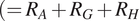 $ \Big(={R}_A+{R}_G+{R}_H $
); and
$ \Big(={R}_A+{R}_G+{R}_H $
); and
 $ {p}_A={R}_A/{R}_S $
(unitless).
$ {p}_A={R}_A/{R}_S $
(unitless).

Similarly, Figure 7 presents
 $ {p}_A $
together with the proportion of
$ {p}_A $
together with the proportion of
 $ {R}_G $
to
$ {R}_G $
to
 $ {R}_S $
and
$ {R}_S $
and
 $ {R}_H $
to
$ {R}_H $
to
 $ {R}_S $
(denoted as
$ {R}_S $
(denoted as
 $ {p}_G $
, and
$ {p}_G $
, and
 $ {p}_H $
, respectively) for each model and chronosequence site. Periods without data (approximately January–April and October–December) correspond to when soils are frozen, during which we assume that
$ {p}_H $
, respectively) for each model and chronosequence site. Periods without data (approximately January–April and October–December) correspond to when soils are frozen, during which we assume that
 $ {R}_A $
equals zero. Computing
$ {R}_A $
equals zero. Computing
 $ {p}_A $
provides a standardized measure that facilitates cross-site comparisons of respiration partitioning with other ecosystems (Jian et al., Reference Jian, Frissell, Hao, Tang, Berryman and Bond-Lamberty2022b), which we discuss in Section 4.2.
$ {p}_A $
provides a standardized measure that facilitates cross-site comparisons of respiration partitioning with other ecosystems (Jian et al., Reference Jian, Frissell, Hao, Tang, Berryman and Bond-Lamberty2022b), which we discuss in Section 4.2.
Forward model results of the annual proportion of components of soil respiration for each of the submodels (Null, Microbe, and Quality) and depth of soil temperature measurements (5 or 10 cm). Proportions were computed with soil respiration using the median values from Figure 6.
 $ {p}_A $
: proportion of autotrophic respiration (yellow);
$ {p}_A $
: proportion of autotrophic respiration (yellow);
 $ {p}_G $
: proportion of heterotrophic growth respiration (purple);
$ {p}_G $
: proportion of heterotrophic growth respiration (purple);
 $ {p}_H $
: proportion of heterotrophic maintenance respiration (blue). We assume
$ {p}_H $
: proportion of heterotrophic maintenance respiration (blue). We assume
 $ {p}_A $
is zero in freezing soils, so results are only shown when
$ {p}_A $
is zero in freezing soils, so results are only shown when
 $ {p}_A>0 $
, considered to be the active growing season (approximately April–October).
$ {p}_A>0 $
, considered to be the active growing season (approximately April–October).

Notably, the annual pattern in
 $ {R}_A $
and
$ {R}_A $
and
 $ {p}_A $
in Figures 6 and 7 for the 2012 chronosequence site displayed a longer period during which
$ {p}_A $
in Figures 6 and 7 for the 2012 chronosequence site displayed a longer period during which
 $ {R}_A $
and
$ {R}_A $
and
 $ {p}_A $
remained near zero before reaching a seasonal peak. This pattern is consistent with the environmental inputs of
$ {p}_A $
remained near zero before reaching a seasonal peak. This pattern is consistent with the environmental inputs of
 $ SWC $
and
$ SWC $
and
 $ {F}_{GPP} $
(Figure 2), which directly influence
$ {F}_{GPP} $
(Figure 2), which directly influence
 $ {R}_A $
through
$ {R}_A $
through
 $ {g}_R $
(Equation 2.2, driven by
$ {g}_R $
(Equation 2.2, driven by
 $ SWC $
) and
$ SWC $
) and
 $ {F}_{GPP} $
(Equation 2.1). At the 2012 site,
$ {F}_{GPP} $
(Equation 2.1). At the 2012 site,
 $ {F}_{GPP} $
was lower overall, and in early summer
$ {F}_{GPP} $
was lower overall, and in early summer
 $ SWC $
declined to zero, thereby suppressing
$ SWC $
declined to zero, thereby suppressing
 $ {R}_A $
and
$ {R}_A $
and
 $ {p}_A $
.
$ {p}_A $
.
A factor influencing
 $ {R}_A $
(and by association
$ {R}_A $
(and by association
 $ {p}_A $
) at all sites is the function
$ {p}_A $
) at all sites is the function
 $ h(SWC) $
(Equation 2.2; Moyano et al. [Reference Moyano, Manzoni and Chenu2013]). This function reaches an optimum near unity when
$ h(SWC) $
(Equation 2.2; Moyano et al. [Reference Moyano, Manzoni and Chenu2013]). This function reaches an optimum near unity when
 $ SWC=0.64 $
, and decreases when
$ SWC=0.64 $
, and decreases when
 $ SWC>0.64 $
, thereby reducing
$ SWC>0.64 $
, thereby reducing
 $ {R}_A $
. In early spring at the 1990, 1968, and Control sites,
$ {R}_A $
. In early spring at the 1990, 1968, and Control sites,
 $ SWC $
remains closer to this optimum (Figure 2), which helps explain higher
$ SWC $
remains closer to this optimum (Figure 2), which helps explain higher
 $ {R}_A $
values during that period. Additionally, to verify that our implementation of
$ {R}_A $
values during that period. Additionally, to verify that our implementation of
 $ h(SWC) $
did not unduly influence these patterns, we repeated the parameter estimation with
$ h(SWC) $
did not unduly influence these patterns, we repeated the parameter estimation with
 $ h(SWC)=1 $
and
$ h(SWC)=1 $
and
 $ h(SWC)= SWC $
. The resulting model outputs are shown in Figures 6 and 7 of the Supplementary Information exhibited no early-season suppression of
$ h(SWC)= SWC $
. The resulting model outputs are shown in Figures 6 and 7 of the Supplementary Information exhibited no early-season suppression of
 $ {R}_A $
(and by association
$ {R}_A $
(and by association
 $ {p}_A $
) at the 2012 site, while the overall seasonal patterns remained consistent.
$ {p}_A $
) at the 2012 site, while the overall seasonal patterns remained consistent.
To independently corroborate our parameter estimates and model results, we used submodel evaluations to compute the distribution of annual cumulative litterfall (
 $ ={L}_T+{L}_{VP}+{L}_{ML} $
) and total annual soil carbon fluxes and their components (Table 2 in the Supplementary Information). We then compared these outputs against three empirical relationships established in the literature: (1) annual litterfall versus total soil respiration (
$ ={L}_T+{L}_{VP}+{L}_{ML} $
) and total annual soil carbon fluxes and their components (Table 2 in the Supplementary Information). We then compared these outputs against three empirical relationships established in the literature: (1) annual litterfall versus total soil respiration (
 $ {R}_S $
) (Davidson et al., Reference Davidson, Savage, Bolstad, Clark, Curtis, Ellsworth, Hanson, Law, Luo, Pregitzer, Randolph and Zak2002), (2) heterotrophic respiration (
$ {R}_S $
) (Davidson et al., Reference Davidson, Savage, Bolstad, Clark, Curtis, Ellsworth, Hanson, Law, Luo, Pregitzer, Randolph and Zak2002), (2) heterotrophic respiration (
 $ {R}_H $
) versus total soil respiration (Bond-Lamberty et al., Reference Bond-Lamberty, Wang and Gower2004b), and (3) autotrophic respiration proportion (
$ {R}_H $
) versus total soil respiration (Bond-Lamberty et al., Reference Bond-Lamberty, Wang and Gower2004b), and (3) autotrophic respiration proportion (
 $ {p}_A $
) versus total soil respiration (Subke et al., Reference Subke, Inglima and Cotrufo2006). We also evaluated linear regression statistics from the modeled results for each relationship (Figure 8).
$ {p}_A $
) versus total soil respiration (Subke et al., Reference Subke, Inglima and Cotrufo2006). We also evaluated linear regression statistics from the modeled results for each relationship (Figure 8).
Associations between annual soil respiration components, cumulative litterfall, and the proportion of autotrophic respiration compared to parameterization at either the 5 cm or 10 cm depth and the soil carbon submodel studied. For each scatterplot, boxes represent the 25–75% distribution of a covariate, and whiskers represent the minimum or maximum of a measurement, with points representing the median value, as reported in the Supplementary Information. Since
 $ {R}_A $
is zero for freezing soils, values of
$ {R}_A $
is zero for freezing soils, values of
 $ {p}_A $
are computed during the active growing season (approximately April–October). For comparison, previously reported empirical relationships are represented. (a):
$ {p}_A $
are computed during the active growing season (approximately April–October). For comparison, previously reported empirical relationships are represented. (a):
 $ {R}_S=161+3.61{L}_T $
, Davidson et al. (Reference Davidson, Savage, Bolstad, Clark, Curtis, Ellsworth, Hanson, Law, Luo, Pregitzer, Randolph and Zak2002); (b):
$ {R}_S=161+3.61{L}_T $
, Davidson et al. (Reference Davidson, Savage, Bolstad, Clark, Curtis, Ellsworth, Hanson, Law, Luo, Pregitzer, Randolph and Zak2002); (b):
 $ \ln \left({R}_H\right)=0.22+0.87\ln \left({R}_S\right) $
, Bond-Lamberty et al. (Reference Bond-Lamberty, Wang and Gower2004b) and Bond-Lamberty and Thomson (Reference Bond-Lamberty and Thomson2010); (c):
$ \ln \left({R}_H\right)=0.22+0.87\ln \left({R}_S\right) $
, Bond-Lamberty et al. (Reference Bond-Lamberty, Wang and Gower2004b) and Bond-Lamberty and Thomson (Reference Bond-Lamberty and Thomson2010); (c):
 $ {p}_A=-0.482+0.138\ln \left({R}_S\right) $
, Subke et al. (Reference Subke, Inglima and Cotrufo2006).
$ {p}_A=-0.482+0.138\ln \left({R}_S\right) $
, Subke et al. (Reference Subke, Inglima and Cotrufo2006).

In Figure 8a, all models showed strong visual agreement with the empirical relationship established by Davidson et al. (Reference Davidson, Savage, Bolstad, Clark, Curtis, Ellsworth, Hanson, Law, Luo, Pregitzer, Randolph and Zak2002) (
 $ {R}_S=161+3.61{L}_T $
). This visual agreement was supported by simple linear regression, which indicated significant associations across all submodels and depths (
$ {R}_S=161+3.61{L}_T $
). This visual agreement was supported by simple linear regression, which indicated significant associations across all submodels and depths (
 $ p<.05 $
). The Microbe submodel at 10 cm depth exhibited the lowest regression RMSE among all models (71 g C m
$ p<.05 $
). The Microbe submodel at 10 cm depth exhibited the lowest regression RMSE among all models (71 g C m
 $ {}^{-2} $
yr
$ {}^{-2} $
yr
 $ {}^{-1} $
).
$ {}^{-1} $
).
For Figure 8b, the Null submodel overestimated
 $ {R}_H $
relative to the expected empirical relationship (
$ {R}_H $
relative to the expected empirical relationship (
 $ \ln \left({R}_H\right)=0.22+0.87\ln \left({R}_S\right) $
; Bond-Lamberty et al. (Reference Bond-Lamberty, Wang and Gower2004b), Bond-Lamberty and Thomson [Reference Bond-Lamberty and Thomson2010]). This overestimation likely occurs because the Null submodel does not separate heterotrophic respiration into
$ \ln \left({R}_H\right)=0.22+0.87\ln \left({R}_S\right) $
; Bond-Lamberty et al. (Reference Bond-Lamberty, Wang and Gower2004b), Bond-Lamberty and Thomson [Reference Bond-Lamberty and Thomson2010]). This overestimation likely occurs because the Null submodel does not separate heterotrophic respiration into
 $ {R}_G $
and
$ {R}_G $
and
 $ {R}_H $
, whereas the Microbe and Quality submodels separately describe
$ {R}_H $
, whereas the Microbe and Quality submodels separately describe
 $ {R}_G $
and
$ {R}_G $
and
 $ {R}_H $
(Equations 2.5 and 2.6, respectively). Linear regression indicated that most submodels and depths were significantly associated (
$ {R}_H $
(Equations 2.5 and 2.6, respectively). Linear regression indicated that most submodels and depths were significantly associated (
 $ p<.05 $
), except for the Quality model at 5 cm depth. The Microbe submodel at 10 cm depth again had the lowest regression RMSE (1.1 g C m
$ p<.05 $
), except for the Quality model at 5 cm depth. The Microbe submodel at 10 cm depth again had the lowest regression RMSE (1.1 g C m
 $ {}^{-2} $
yr
$ {}^{-2} $
yr
 $ {}^{-1} $
at 5 cm depth after converting from
$ {}^{-1} $
at 5 cm depth after converting from
 $ \ln \left({R}_H\right) $
to
$ \ln \left({R}_H\right) $
to
 $ {R}_H $
).
$ {R}_H $
).
Finally, Figure 8c shows that all models underestimated
 $ {p}_A $
relative to the expected empirical relationship (
$ {p}_A $
relative to the expected empirical relationship (
 $ {p}_A=-0.482+0.138\ln \left({R}_S\right) $
; Subke et al. [Reference Subke, Inglima and Cotrufo2006]). This outcome is consistent with the absence of significant associations between
$ {p}_A=-0.482+0.138\ln \left({R}_S\right) $
; Subke et al. [Reference Subke, Inglima and Cotrufo2006]). This outcome is consistent with the absence of significant associations between
 $ \ln \left({R}_H\right) $
and
$ \ln \left({R}_H\right) $
and
 $ {p}_A $
for any submodel or depth. RMSE values for all submodels ranged from 0.32 to 0.33.
$ {p}_A $
for any submodel or depth. RMSE values for all submodels ranged from 0.32 to 0.33.
4. Discussion
The objective of this study was to model and characterize annual patterns of soil respiration components across a fire chronosequence. Measuring soil respiration with chamber-based methods or the flux-gradient approach is inherently challenging (Maier and Schack-Kirchner, Reference Maier and Schack-Kirchner2014), and even more so for the remote sites in this study. The remoteness and access to our sites confined the period of data collection to one month, which we compensated for using a factorial design approach (4 sites, 3 models, 2 depths) for model analysis and evaluation.
All submodels produced annual patterns of soil respiration (and their associated components) across the fire chronosequence (Figures 6 and 7). We used the median for parameter optimization and modeled fluxes because it reduces the influence of outliers (Devore et al., Reference Devore, Berk and Carlton2021) and intra-site variation, improving comparability across the chronosequence. After evaluating the parameter estimation method, we examine how chronosequence site and submodel structure influence model parameterization and outputs. Finally, we assess the extent to which the Microbe and Quality submodels better replicate modeled components of soil respiration compared to the Null submodel.
4.1. Evaluation of modeling approach and parameter estimation method
We applied a quasi-steady-state assumption to derive empirical equations for respiration fluxes (
 $ {R}_A $
,
$ {R}_A $
,
 $ {R}_H $
, and
$ {R}_H $
, and
 $ {R}_G $
), enabling direct identification of parameters influencing soil respiration (Equations 2.4–2.6). This assumption reduces model complexity (Carvalhais et al., Reference Carvalhais, Reichstein, Seixas, Collatz, Pereira, Berbigier, Carrara, Granier, Montagnani, Papale, Rambal, Sanz and Valentini2008; Todd-Brown et al., Reference Todd-Brown, Hopkins, Kivlin, Talbot and Allison2012; Ryan et al., Reference Ryan, Ogle, Kropp, Samuels-Crow, Carrillo and Pendall2018) and computational bottlenecks (Xia et al., Reference Xia, Luo, Wang, Weng and Hararuk2012; Fang et al., Reference Fang, Liu, Huang, Li and Leung2014; Fer et al., Reference Fer, Kelly, Moorcroft, Richardson, Cowdery and Dietze2018; Wiltshire et al., Reference Wiltshire, Grobe and Beckage2023), making sensitivity analyses more tractable (Figures 4–7), especially for the multiple sites and models analyzed in this study.
$ {R}_G $
), enabling direct identification of parameters influencing soil respiration (Equations 2.4–2.6). This assumption reduces model complexity (Carvalhais et al., Reference Carvalhais, Reichstein, Seixas, Collatz, Pereira, Berbigier, Carrara, Granier, Montagnani, Papale, Rambal, Sanz and Valentini2008; Todd-Brown et al., Reference Todd-Brown, Hopkins, Kivlin, Talbot and Allison2012; Ryan et al., Reference Ryan, Ogle, Kropp, Samuels-Crow, Carrillo and Pendall2018) and computational bottlenecks (Xia et al., Reference Xia, Luo, Wang, Weng and Hararuk2012; Fang et al., Reference Fang, Liu, Huang, Li and Leung2014; Fer et al., Reference Fer, Kelly, Moorcroft, Richardson, Cowdery and Dietze2018; Wiltshire et al., Reference Wiltshire, Grobe and Beckage2023), making sensitivity analyses more tractable (Figures 4–7), especially for the multiple sites and models analyzed in this study.
Dynamic process models (Sacks et al., Reference Sacks, Schimel, Monson and Braswell2006; Zobitz et al., Reference Zobitz, Moore, Sacks, Monson, Bowling and Schimel2008) require explicit representation of carbon pools (
 $ {C}_S $
,
$ {C}_S $
,
 $ {C}_R $
,
$ {C}_R $
,
 $ {C}_M $
, and
$ {C}_M $
, and
 $ {C}_A $
); parameter estimation with these process models are best constrained with repeated measurements of root, soil, or microbial stocks. As such observations were unavailable for this study, the quasi–steady-state approach we adopted is a compromise between data availability and model complexity. Nevertheless, incorporating measured carbon stock data in future work could help reduce parameter uncertainty and improve model-data comparisons (Richardson et al., Reference Richardson, Williams, Hollinger, Moore, Dail, Davidson, Scott, Evans, Hughes, Lee, Rodrigues and Savage2010).
$ {C}_A $
); parameter estimation with these process models are best constrained with repeated measurements of root, soil, or microbial stocks. As such observations were unavailable for this study, the quasi–steady-state approach we adopted is a compromise between data availability and model complexity. Nevertheless, incorporating measured carbon stock data in future work could help reduce parameter uncertainty and improve model-data comparisons (Richardson et al., Reference Richardson, Williams, Hollinger, Moore, Dail, Davidson, Scott, Evans, Hughes, Lee, Rodrigues and Savage2010).
Despite these limitations, the MCMC method effectively characterized the posterior likelihood distribution at all sites and models (Table 2 and Figures 4 and 5 in the Supplementary Information), with the widest posterior distribution at the 1968 chronosequence site, also reflected as the site with the widest violin plot (Figure 5). The depth at which soil temperature was measured did not meaningfully impact the parameter estimation and consequently the annual cycle of soil respiration components (Figures 6 and 7).
Although we sought to maximize the information content of the field measurements, the limited number of observations at each chronosequence site constrains the extent to which the model results in Figure 6 can be generalized. In this context, the estimated parameters should be viewed as (1) guiding intuition for model behavior, (2) identifying constraints on the model structure, and (3) evaluating whether parameter ranges narrower than those summarized in Table 1 are supported by the data. Future applications incorporating longer time series or repeated seasonal sampling into the MCMC framework would enable more robust evaluation of the model (Braswell et al., Reference Braswell, Sacks, Linder and Schimel2005), perhaps with increased computational cost.
4.2. Chronosequence effects on parameterization and model results
A key question of this study was to examine the sensitivity of model parameters to time since fire disturbance or chronosequence age. One approach to evaluate associations between chronosequence site and model parameters is through investigation of the distribution of accepted parameter values using chronosequence age as a covariate (Figure 4). Chronosequence age strongly influenced parameters related to litterfall rates (
 $ {L}_T $
,
$ {L}_T $
,
 $ {L}_{VP} $
,
$ {L}_{VP} $
,
 $ {L}_{ML} $
). In contrast, root turnover (
$ {L}_{ML} $
). In contrast, root turnover (
 $ {\delta}_R $
) showed little sensitivity to age, despite playing a similar functional role in increasing soil carbon substrate (Figure 3). The
$ {\delta}_R $
) showed little sensitivity to age, despite playing a similar functional role in increasing soil carbon substrate (Figure 3). The
 $ {r}_1 $
and
$ {r}_1 $
and
 $ {r}_2 $
parameters in the Quality submodel showed different trends across the chronosequence depending on the soil temperature measurement depth. However, this sensitivity did not meaningfully affect model–data agreement (Figure 5) or comparisons to empirical patterns in respiration components (Figures 8b–c). Other Microbe and Quality submodel parameters showed little sensitivity to chronosequence age.
$ {r}_2 $
parameters in the Quality submodel showed different trends across the chronosequence depending on the soil temperature measurement depth. However, this sensitivity did not meaningfully affect model–data agreement (Figure 5) or comparisons to empirical patterns in respiration components (Figures 8b–c). Other Microbe and Quality submodel parameters showed little sensitivity to chronosequence age.
We found significant association between inferred annual litterfall rates to soil respiration consistent with previously established empirical patterns between litterfall rates and respiration (Figure 8a; Davidson et al. [Reference Davidson, Savage, Bolstad, Clark, Curtis, Ellsworth, Hanson, Law, Luo, Pregitzer, Randolph and Zak2002]). The sensitivity of litterfall rates with soil respiration (and therefore chronosequence age) also conforms with expectations from observational studies. Soil respiration and litterfall rates are directly associated with each other (Reynolds and Hunter, Reference Reynolds and Hunter2001; Subke et al., Reference Subke, Hahn, Battipaglia, Linder, Buchmann and Cotrufo2004; Wei and Man, Reference Wei and Man2021; Paré et al., Reference Paré, Laganière, Larocque and Boutin2022). These litterfall rates also increase following recovery from fire disturbance (Grigal and McColl, Reference Grigal and McColl1975).
Parameter estimates of
 $ {\delta}_R $
were not sensitive to chronosequence age (Figure 4), which was contrary to our expectations for three reasons. First, previous investigations at these same sites reported associations between soil moisture, root biomass, and time since the fire occurred (Aaltonen et al., Reference Aaltonen, Köster, Köster, Berninger, Zhou, Karhu, Biasi, Bruckman, Palviainen and Pumpanen2019a, Reference Aaltonen, Palviainen, Zhou, Köster, Berninger, Pumpanen and Köster2019b). Second, previous studies have established links between root turnover and soil respiration. Adamczyk et al. (Reference Adamczyk, Rüthi and Frey2021) found that root exudates are positively associated with microbial abundance and diversity, and coincidentally impact overall soil respiration. Similarly, Finér et al. (Reference Finér, Ohashi, Noguchi and Hirano2011) showed that fine root biomass can be sensitive to temperature, soil moisture, or either environmental factors. Third, root turnover (
$ {\delta}_R $
were not sensitive to chronosequence age (Figure 4), which was contrary to our expectations for three reasons. First, previous investigations at these same sites reported associations between soil moisture, root biomass, and time since the fire occurred (Aaltonen et al., Reference Aaltonen, Köster, Köster, Berninger, Zhou, Karhu, Biasi, Bruckman, Palviainen and Pumpanen2019a, Reference Aaltonen, Palviainen, Zhou, Köster, Berninger, Pumpanen and Köster2019b). Second, previous studies have established links between root turnover and soil respiration. Adamczyk et al. (Reference Adamczyk, Rüthi and Frey2021) found that root exudates are positively associated with microbial abundance and diversity, and coincidentally impact overall soil respiration. Similarly, Finér et al. (Reference Finér, Ohashi, Noguchi and Hirano2011) showed that fine root biomass can be sensitive to temperature, soil moisture, or either environmental factors. Third, root turnover (
 $ {\delta}_R{C}_R $
; dashed line in Roots, Figure 3; Equation 5.2, Supplementary Information) and root exudation (
$ {\delta}_R{C}_R $
; dashed line in Roots, Figure 3; Equation 5.2, Supplementary Information) and root exudation (
 $ \beta {F}_{GPP} $
, Equation 5.4, Supplementary Information) transfer carbon from the root pool to the soil pool. Root turnover and exudation appear in the quasi-steady state expression for
$ \beta {F}_{GPP} $
, Equation 5.4, Supplementary Information) transfer carbon from the root pool to the soil pool. Root turnover and exudation appear in the quasi-steady state expression for
 $ {R}_A $
(Equation 2.1). Given these connections among disturbance history, root activity, and model representation of
$ {R}_A $
(Equation 2.1). Given these connections among disturbance history, root activity, and model representation of
 $ {\delta}_R $
, we would have expected
$ {\delta}_R $
, we would have expected
 $ {\delta}_R $
to vary across the chronosequence.
$ {\delta}_R $
to vary across the chronosequence.
This insensitivity in
 $ {\delta}_R $
is a contributing factor for the weak association between modeled
$ {\delta}_R $
is a contributing factor for the weak association between modeled
 $ {p}_A $
and observed
$ {p}_A $
and observed
 $ \ln \left({R}_S\right) $
(Figure 8c). Our modeled
$ \ln \left({R}_S\right) $
(Figure 8c). Our modeled
 $ {p}_A $
values were lower than those predicted by the empirical relationship from Subke et al. (Reference Subke, Inglima and Cotrufo2006). Similarly, Jian et al. (Reference Jian, Frissell, Hao, Tang, Berryman and Bond-Lamberty2022b), in a global synthesis study from the Soil Respiration Database (SRDB), reported
$ {p}_A $
values were lower than those predicted by the empirical relationship from Subke et al. (Reference Subke, Inglima and Cotrufo2006). Similarly, Jian et al. (Reference Jian, Frissell, Hao, Tang, Berryman and Bond-Lamberty2022b), in a global synthesis study from the Soil Respiration Database (SRDB), reported
 $ {p}_A $
to range
$ {p}_A $
to range
 $ 0.42\pm 0.18 $
, without clear trends across ecosystem types. The reported range from Jian et al. (Reference Jian, Frissell, Hao, Tang, Berryman and Bond-Lamberty2022b) is within the uncertainty of
$ 0.42\pm 0.18 $
, without clear trends across ecosystem types. The reported range from Jian et al. (Reference Jian, Frissell, Hao, Tang, Berryman and Bond-Lamberty2022b) is within the uncertainty of
 $ {p}_A $
in Figure 8c and during the peak growing season in Figures 6 and 7. Overall, these findings suggest our submodels oversimplify root carbon dynamics.
$ {p}_A $
in Figure 8c and during the peak growing season in Figures 6 and 7. Overall, these findings suggest our submodels oversimplify root carbon dynamics.
We anticipate that the additional data collection—focused on better understanding of
 $ {\delta}_R $
—would feed forward into model refinement and improvement. Systematic surveys of root biomass during different periods in the year could help elucidate which environmental factors (e.g.
$ {\delta}_R $
—would feed forward into model refinement and improvement. Systematic surveys of root biomass during different periods in the year could help elucidate which environmental factors (e.g.
 $ GPP $
or
$ GPP $
or
 $ NPP $
) (Ruess et al., Reference Ruess, Hendrick, Burton, Pregitzer, Sveinbjornssön, Allen and Maurer2003) facilitate root growth, exudation, and turnover at particular chronosequence sites. With that information, models of root exudates could be time-dependent or associated with environmental forcing variables.
$ NPP $
) (Ruess et al., Reference Ruess, Hendrick, Burton, Pregitzer, Sveinbjornssön, Allen and Maurer2003) facilitate root growth, exudation, and turnover at particular chronosequence sites. With that information, models of root exudates could be time-dependent or associated with environmental forcing variables.
Model refinement of root turnover would have secondary impacts on
 $ {p}_A $
. The quasi-steady state expressions formulated for the FireGrow model establish direct relationships between model outputs (
$ {p}_A $
. The quasi-steady state expressions formulated for the FireGrow model establish direct relationships between model outputs (
 $ {R}_A $
,
$ {R}_A $
,
 $ {R}_G $
, and
$ {R}_G $
, and
 $ {R}_H $
) and model parameters. In Equation 2.1,
$ {R}_H $
) and model parameters. In Equation 2.1,
 $ {R}_A $
, and hence
$ {R}_A $
, and hence
 $ {p}_A $
increases when
$ {p}_A $
increases when
 $ {\delta}_R $
decreases. Model improvement for the structural consideration of root carbon dynamics should also consider uncertainties in the association between between
$ {\delta}_R $
decreases. Model improvement for the structural consideration of root carbon dynamics should also consider uncertainties in the association between between
 $ {p}_A $
and
$ {p}_A $
and
 $ {R}_S $
. Jian et al. (Reference Jian, Frissell, Hao, Tang, Berryman and Bond-Lamberty2022b) also concluded that
$ {R}_S $
. Jian et al. (Reference Jian, Frissell, Hao, Tang, Berryman and Bond-Lamberty2022b) also concluded that
 $ {R}_S $
explains 2% of the variability on
$ {R}_S $
explains 2% of the variability on
 $ {p}_A $
. Given the methodological challenges of direct measurement of
$ {p}_A $
. Given the methodological challenges of direct measurement of
 $ {p}_A $
(Hanson et al., Reference Hanson, Edwards, Garten and Andrews2000), uncertainty reduction in model estimates of
$ {p}_A $
(Hanson et al., Reference Hanson, Edwards, Garten and Andrews2000), uncertainty reduction in model estimates of
 $ {p}_A $
could occur through (1) inferring root turnover rates from measurable aboveground indicators (such as aboveground leaf or needle turnover rates [Sloan et al., Reference Sloan, Fletcher, Press, Williams and Phoenix2013]); or (2) separation of different root classes (e.g. fine roots versus coarse roots [Kalyn and Van Rees, Reference Kalyn and Van Rees2006; Finér et al., Reference Finér, Ohashi, Noguchi and Hirano2011; Neumann et al., Reference Neumann, Godbold, Hirano and Finér2020].
$ {p}_A $
could occur through (1) inferring root turnover rates from measurable aboveground indicators (such as aboveground leaf or needle turnover rates [Sloan et al., Reference Sloan, Fletcher, Press, Williams and Phoenix2013]); or (2) separation of different root classes (e.g. fine roots versus coarse roots [Kalyn and Van Rees, Reference Kalyn and Van Rees2006; Finér et al., Reference Finér, Ohashi, Noguchi and Hirano2011; Neumann et al., Reference Neumann, Godbold, Hirano and Finér2020].
4.3. Structured models of soil carbon better replicate modeled components of soil respiration
Figures 6 and 7 do not suggest any meaningful submodel differences between parameterization depth (5 or 10 cm). We also did not find any meaningful differences between different implementations of
 $ h(SWC) $
beyond Equation 2.2 (see Supplementary Information). The lack of sensitivity to parameterization depth was unexpected, given the depth-specific differences in
$ h(SWC) $
beyond Equation 2.2 (see Supplementary Information). The lack of sensitivity to parameterization depth was unexpected, given the depth-specific differences in
 $ {Q}_{10,R} $
(Table 1), but was likely offset by similar temperature profiles across depths at all chronosequence sites (Figure 2). The largest temperature gradient between depths (approximately 2 °C) occurred in midsummer at the Control site, though its effect on modeled respiration was likely marginal. We attribute this pattern to ground cover re-insulation, which reduces active layer thickness and steepens the soil temperature gradient (Köster et al., Reference Köster, Köster, Berninger, Aaltonen, Zhou and Pumpanen2017; Aaltonen et al., Reference Aaltonen, Köster, Köster, Berninger, Zhou, Karhu, Biasi, Bruckman, Palviainen and Pumpanen2019a, Reference Aaltonen, Palviainen, Zhou, Köster, Berninger, Pumpanen and Köster2019b).
$ {Q}_{10,R} $
(Table 1), but was likely offset by similar temperature profiles across depths at all chronosequence sites (Figure 2). The largest temperature gradient between depths (approximately 2 °C) occurred in midsummer at the Control site, though its effect on modeled respiration was likely marginal. We attribute this pattern to ground cover re-insulation, which reduces active layer thickness and steepens the soil temperature gradient (Köster et al., Reference Köster, Köster, Berninger, Aaltonen, Zhou and Pumpanen2017; Aaltonen et al., Reference Aaltonen, Köster, Köster, Berninger, Zhou, Karhu, Biasi, Bruckman, Palviainen and Pumpanen2019a, Reference Aaltonen, Palviainen, Zhou, Köster, Berninger, Pumpanen and Köster2019b).
In Figure 6, the Null submodel consistently overestimates
 $ {R}_H $
across daily (and consequently) annual timescales; we attribute this overestimation to its formulation (Equation 2.4) that does not separately represent
$ {R}_H $
across daily (and consequently) annual timescales; we attribute this overestimation to its formulation (Equation 2.4) that does not separately represent
 $ {R}_G $
and
$ {R}_G $
and
 $ {R}_H $
. This overestimation is further reflected in the weaker empirical association between
$ {R}_H $
. This overestimation is further reflected in the weaker empirical association between
 $ {R}_H $
and
$ {R}_H $
and
 $ {R}_S $
(Figure 7b), compared to the Microbe and Quality submodels. In contrast, the Microbe and Quality submodels show broadly similar performance (Figures 6, 7), even though they differ in their representations of
$ {R}_S $
(Figure 7b), compared to the Microbe and Quality submodels. In contrast, the Microbe and Quality submodels show broadly similar performance (Figures 6, 7), even though they differ in their representations of
 $ {R}_G $
and
$ {R}_G $
and
 $ {R}_H $
(Equations 2.5 and 2.6). These results indicate that explicitly incorporating microbial processes provides a more accurate characterization of soil respiration components, even if structural differences among submodels produce comparable outcomes. While untested here, relaxing the quasi–steady-state assumption may further distinguish the Microbe and Quality submodels, but doing so would require additional observations of pool sizes or inferring litterfall rates from measured litterfall as previously discussed.
$ {R}_H $
(Equations 2.5 and 2.6). These results indicate that explicitly incorporating microbial processes provides a more accurate characterization of soil respiration components, even if structural differences among submodels produce comparable outcomes. While untested here, relaxing the quasi–steady-state assumption may further distinguish the Microbe and Quality submodels, but doing so would require additional observations of pool sizes or inferring litterfall rates from measured litterfall as previously discussed.
While model structure and microbial representation explain part of the variability in
 $ {R}_H $
, external site factors, such as fire history, also influence soil respiration dynamics. Kelly et al. (Reference Kelly, Ibáñez, Santín, Doerr, Nilsson, Holst, Lindroth and Kljun2021) identified autotrophic respiration and nutrient pulses following fire disturbances as key drivers of soil respiration. While fire intensity is also an important factor influencing post-fire soil dynamics (Ribeiro-Kumara et al., Reference Ribeiro-Kumara, Köster, Aaltonen and Köster2020; Kelly et al., Reference Kelly, Ibáñez, Santín, Doerr, Nilsson, Holst, Lindroth and Kljun2021), all our sites experienced a stand-replacing fire, which we assume to be of equal fire intensity. Differences in fire severity or burn conditions across chronosequence sites could contribute to some of the observed variation in soil respiration rates; future work could elucidate the relative contributions of burn severity and time since disturbance to measured soil respiration.
$ {R}_H $
, external site factors, such as fire history, also influence soil respiration dynamics. Kelly et al. (Reference Kelly, Ibáñez, Santín, Doerr, Nilsson, Holst, Lindroth and Kljun2021) identified autotrophic respiration and nutrient pulses following fire disturbances as key drivers of soil respiration. While fire intensity is also an important factor influencing post-fire soil dynamics (Ribeiro-Kumara et al., Reference Ribeiro-Kumara, Köster, Aaltonen and Köster2020; Kelly et al., Reference Kelly, Ibáñez, Santín, Doerr, Nilsson, Holst, Lindroth and Kljun2021), all our sites experienced a stand-replacing fire, which we assume to be of equal fire intensity. Differences in fire severity or burn conditions across chronosequence sites could contribute to some of the observed variation in soil respiration rates; future work could elucidate the relative contributions of burn severity and time since disturbance to measured soil respiration.
Incorporating soil microbial processes into soil models can improve model–data agreement for soil respiration (Wutzler and Reichstein, Reference Wutzler and Reichstein2013; Taş et al., Reference Taş, Prestat, McFarland, Wickland, Knight, Berhe, Jorgenson, Waldrop and Jansson2014; Woolf and Lehmann, Reference Woolf and Lehmann2019; Pierson et al., Reference Pierson, Lohse, Wieder, Patton, Facer, de Graaff, Georgiou, Seyfried, Flerchinger and Will2022). Neglecting these dynamics or not including microbial interactions with soil carbon may lead to underestimation of projected climate responses, particularly in permafrost regions (Fan et al., Reference Fan, Jastrow, Liang, Matamala and Miller2013; Perveen et al., Reference Perveen, Barot, Alvarez, Klumpp, Martin, Rapaport, Herfurth, Louault and Fontaine2014; Keuper et al., Reference Keuper, Wild, Kummu, Beer, Blume-Werry, Fontaine, Gavazov, Gentsch, Guggenberger, Hugelius, Jalava, Koven, Krab, Kuhry, Monteux, Richter, Shahzad, Weedon and Dorrepaal2020). Additional factors, such as long-term shifts in microbial community composition due to the presence or absence of snow cover (Männistö et al., Reference Männistö, Vuosku, Stark, Saravesi, Suokas, Markkola, Martz and Rautio2018), may further influence respiration patterns. Iterative model refinement at affected sites may require seasonal parameter adjustments (Sacks et al., Reference Sacks, Schimel, Monson and Braswell2006; Zobitz et al., Reference Zobitz, Moore, Sacks, Monson, Bowling and Schimel2008) or explicit representation of frozen and thawed carbon pools (Schaefer and Jafarov, Reference Schaefer and Jafarov2016). These microbial processes interact with the physical and structural characteristics of soils, highlighting the need to consider both abiotic and biotic factors when modeling soil respiration.
The interactions between climatic variables and the physical and structural characteristics of soil carbon are critical for understanding site-to-site differences in soil respiration (Luo et al., Reference Luo, Wang and Wang2019; Paré et al., Reference Paré, Laganière, Larocque and Boutin2022). Among the driver variables used in our models,
 $ GPP $
and soil water content had the largest site-to-site variability (Figure 2). In Arctic permafrost ecosystems, winter–spring (and associated freeze/thaw cycles) can contribute as much as 5–20% to annual soil respiration (Mikan et al., Reference Mikan, Schimel and Doyle2002; Kurganova et al., Reference Kurganova, Teepe and Loftfield2007; Wang et al., Reference Wang, Liu, Chung, Yu, Mi, Geng, Jing, Wang, Zeng, Cao, Zhao and He2014; Keuper et al., Reference Keuper, Wild, Kummu, Beer, Blume-Werry, Fontaine, Gavazov, Gentsch, Guggenberger, Hugelius, Jalava, Koven, Krab, Kuhry, Monteux, Richter, Shahzad, Weedon and Dorrepaal2020). Although not explicitly tested in this study, we anticipate that freeze–thaw cycles stimulate soil heterotrophic respiration by mobilizing a thawed, highly labile soil carbon pool. These transient dynamics likely influence annual patterns of soil organic carbon accumulation, particularly in regions with short growing seasons constrained by permafrost dynamics and frozen soils. Direct field measurement of
$ GPP $
and soil water content had the largest site-to-site variability (Figure 2). In Arctic permafrost ecosystems, winter–spring (and associated freeze/thaw cycles) can contribute as much as 5–20% to annual soil respiration (Mikan et al., Reference Mikan, Schimel and Doyle2002; Kurganova et al., Reference Kurganova, Teepe and Loftfield2007; Wang et al., Reference Wang, Liu, Chung, Yu, Mi, Geng, Jing, Wang, Zeng, Cao, Zhao and He2014; Keuper et al., Reference Keuper, Wild, Kummu, Beer, Blume-Werry, Fontaine, Gavazov, Gentsch, Guggenberger, Hugelius, Jalava, Koven, Krab, Kuhry, Monteux, Richter, Shahzad, Weedon and Dorrepaal2020). Although not explicitly tested in this study, we anticipate that freeze–thaw cycles stimulate soil heterotrophic respiration by mobilizing a thawed, highly labile soil carbon pool. These transient dynamics likely influence annual patterns of soil organic carbon accumulation, particularly in regions with short growing seasons constrained by permafrost dynamics and frozen soils. Direct field measurement of
 $ {R}_S $
during these spring periods (with subsequent model parameterization) could reduce uncertainty in modeled soil respiration components, offer alternative parameterizations, and improve agreement between measured and modeled
$ {R}_S $
during these spring periods (with subsequent model parameterization) could reduce uncertainty in modeled soil respiration components, offer alternative parameterizations, and improve agreement between measured and modeled
 $ {R}_{S, meas} $
and
$ {R}_{S, meas} $
and
 $ {R}_{S,\mathit{\operatorname{mod}}} $
(Figure 5).
$ {R}_{S,\mathit{\operatorname{mod}}} $
(Figure 5).
5. Conclusion
This study evaluated the ability to parameterize soil respiration models with differing representations of microbial dynamics across a fire chronosequence. All three model variants reproduced expected annual patterns of total soil respiration (
 $ {R}_S $
) consistent with time since fire disturbance. Parameter estimates were generally insensitive to soil depth (5 or 10 cm), indicating that depth had a limited effect on model parameter estimates and modeled soil respiration components. However, models that explicitly represented microbial carbon processes produced stronger model-data comparisons when evaluated against previously established empirical relationships. For our fire chronosequence sites, separate consideration of microbial processes compared to a bulk soil carbon pool is critical to accurately represent microbial contributions to soil carbon cycling; we expect that these findings generalize to other ecosystems. Additionally, parameters associated with aboveground litter inputs displayed variation with chronosequence site, generally consistent with previously observed patterns of vegetation recovery following fire disturbance.
$ {R}_S $
) consistent with time since fire disturbance. Parameter estimates were generally insensitive to soil depth (5 or 10 cm), indicating that depth had a limited effect on model parameter estimates and modeled soil respiration components. However, models that explicitly represented microbial carbon processes produced stronger model-data comparisons when evaluated against previously established empirical relationships. For our fire chronosequence sites, separate consideration of microbial processes compared to a bulk soil carbon pool is critical to accurately represent microbial contributions to soil carbon cycling; we expect that these findings generalize to other ecosystems. Additionally, parameters associated with aboveground litter inputs displayed variation with chronosequence site, generally consistent with previously observed patterns of vegetation recovery following fire disturbance.
Our results demonstrate that satellite-derived gross primary productivity (
 $ {F}_{GPP} $
), soil temperature (
$ {F}_{GPP} $
), soil temperature (
 $ {T}_S $
), and soil water content (
$ {T}_S $
), and soil water content (
 $ SWC $
) can serve as useful substitutes for direct field measurements in modeling soil respiration at remote or data-sparse ecosystems. Based on these findings, we offer three recommendations for future model development and data collection. First, direct field measurements of litterfall and more importantly root turnover rates would reduce model uncertainty by constraining other soil respiration parameters and improving model–data comparisons. Second, targeted sampling during seasonal transition periods (e.g., freeze–thaw cycles) would provide valuable constraints on root turnover and exudation, microbial activity, and respiration dynamics. Third, future versions of the FireGrow model should relax the quasi–steady-state assumption, allowing for explicit coupling between microbial and soil carbon pools and environmental drivers that vary dynamically over the growing season. Future development of soil respiration models will benefit from explicit microbial carbon representation combined with field-based estimates of litterfall and root turnover rates, given that these inputs modulate substrate supply and often serve as a primary control on soil heterotrophic respiration.
$ SWC $
) can serve as useful substitutes for direct field measurements in modeling soil respiration at remote or data-sparse ecosystems. Based on these findings, we offer three recommendations for future model development and data collection. First, direct field measurements of litterfall and more importantly root turnover rates would reduce model uncertainty by constraining other soil respiration parameters and improving model–data comparisons. Second, targeted sampling during seasonal transition periods (e.g., freeze–thaw cycles) would provide valuable constraints on root turnover and exudation, microbial activity, and respiration dynamics. Third, future versions of the FireGrow model should relax the quasi–steady-state assumption, allowing for explicit coupling between microbial and soil carbon pools and environmental drivers that vary dynamically over the growing season. Future development of soil respiration models will benefit from explicit microbial carbon representation combined with field-based estimates of litterfall and root turnover rates, given that these inputs modulate substrate supply and often serve as a primary control on soil heterotrophic respiration.
Open peer review
To view the open peer review materials for this article, please visit http://doi.org/10.1017/eds.2026.10034.
Supplementary material
The supplementary material for this article can be found at http://doi.org/10.1017/eds.2026.10034.
Acknowledgements
We would like the thank feedback from two anonymous reviewers to improve the manuscript. Following initial revisions, select sentences of the text were refined with the assistance of Generative AI to enhance readability. Co-author Zobitz acknowledges B. S. Chelton for helpful discussion on this manuscript.
Author contribution
Conceptualization: J.Z. Methodology: J.Z. (modeling); J.P.; K.K.; F.B. (field data) Software: J.Z. Validation: J.Z. Formal Analysis: J.Z.; F.B. Investigation: J.Z. (modeling); J.P.; K.K.; F.B. (field data); X.Z. (data collection); H.A.; E.K. (experiment, data collection) Data curation: J.Z. Writing – original draft: J.Z. Writing – review and editing: F.B.; K.K.; E.K. Visualization: J.Z. Supervision: J.Z. Project Administration: J.Z. Funding Acquisition: J.Z. (Fulbright).
Competing interests
The authors declare no competing interests.
Data availability statement
The data and R scripts used to execute/report on the analyses in the paper can be found at https://github.com/jmzobitz/FireGrow, and are preserved at https://zenodo.org/doi/10.5281/zenodo.11493787 via Zenodo.
Ethics statement
The research meets all ethical guidelines, including adherence to the legal requirements of the study country.
Funding statement
Co-author Zobitz was funded by the Fulbright Finland Foundation and Saastamoinen Foundation Grant in Health and Environmental Sciences. This work was funded by the Academy of Finland (project numbers 286685, 294600, 307222, 327198, and 337550). Travel funding was provided from EU InterAct (H2020 Grant Agreement No. 730938).


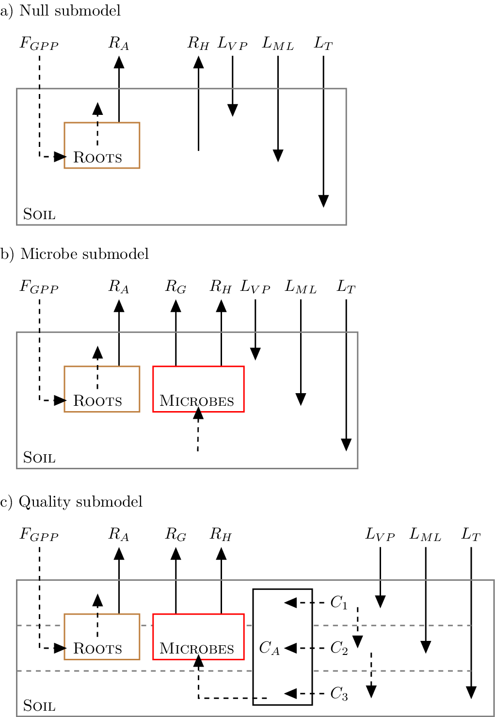


 Open access
Comments
Augsburg University
Tel: 612-330-1068
2211 Riverside Avenue
Minneapolis, MN 55454
zobitz@augsburg.edu
August 15, 2024
Dr. Claire Monteleoni, Editor-in-Chief
University of Colorado, Boulder & INRIA, France
Dear Dr. Monteleoni,
Please consider the enclosed manuscript for publication in Environmental Data Science. The manuscript is entitled, “Combined effects of site and model parameterization for soil respiration components in a Canadian wildfire chronosequence”. Our manuscript parameterizes soil respiration models with data collected along a forest fire chronosequence in Northern Canada. Model outputs are then evaluated by examining annual patterns in respiration outputs and through statistical analyses. We believe this study carefully analyzes the effect of model structure and site differences on the interpretation of model results.
We believe that Environmental Data Science is an excellent venue for publication of this work. One of the Journal’s aims are:
“the use of data-driven approaches to understand environmental processes - including climate change - and aid sustainable decision-making. The data and methodological scope is defined broadly to encompass artificial intelligence, machine learning, data mining, computer vision, econometrics and other statistical techniques.”
Our study illustrates workflows for the collection and harmonization of different data streams (from field level to remote sensing measurements) for a machine learning approach. A factorial approach is applied for model parameter estimation and evaluation. The methods shown here provide a computationally efficient framework for comparative analyses of sites using a common modeling approach. This framework is useful in the absence of access to high performance computing environments. In total, this manuscript contributes to the growing body of literature on the importance of understanding and modeling soil carbon dynamics through modeling in natural environments.
Our study is an application and methods paper relating to permafrost soils. This manuscript is the product of collaboration between an environmental data scientist (Zobitz) and biogeochemists (the other authors). It is a continuation of previous work that parameterized similar soil carbon models using the same chronosequence data (Zobitz et al. 2021, Geoscientific Model Development), but that study focused exclusively on parameterization and not on simulation of dynamic model outputs. This current study is a natural continuation of our previous efforts (and candidly the initial objective when the study was proposed in 2020).
We have archived our input data, processing files, and output on zenodo (https://zenodo.org/doi/10.5281/zenodo.11493787) per the journal guidelines to promote open data and data re-use.
Suggested reviewers for the manuscript include:
- Göran Ågren, Swedish University of Agricultural Sciences, goran.agren@slu.se
- Ben Bond Lamberty, Pacific Northwest National Lab/University of Maryland, bondlamberty@pnnl.gov
- Bill de Groot, Great Lakes Forestry Center, bill.degroot@canada.ca
- Mike Flannigan, University of Alberta, mike.flannigan@ualberta.ca
- Debjani Sihi, Emory University, debjani.sihi@emory.edu
- Sampo Smolander, Princeton University, sampos@princeton.edu
- Kathe Todd-Brown, University of Florida, kathe.toddbrown@essie.ufl.edu
We’ve selected a variety of suggested reviewers with expertise in modeling, soils biogeochemistry, or fire disturbances who we believe will be well-suited to critically evaluate the manuscript.
Please contact us if you have questions or concerns. Thanks very much!
Sincerely,
John M. Zobitz
Professor of Mathematics and Data Science
Augsburg University