2. Fusion reactions

Consider a reaction between ions of species $a$ and $b$ . The boundaries of a rectangular grid in kinetic energy $E$ and polar angle $\theta$ are defined as

(2.1) \begin{align} E_{i-{({1}/{2})}} \leqslant E \leqslant E_{i+{({1}/{2})}}, \, \theta _{j-{({1}/{2})}} \leqslant \theta \leqslant \theta _{j+{({1}/{2})}}, \end{align}

where $i$ and $j$ denote the energy and angular indices, respectively. The volumetric reaction rate (number of reactions per unit volume per unit time) is then given by

(2.2) \begin{align} q^{a,b} = \frac {1}{1+\delta _{a,b}} \sum _{i_1,i_2} \sum _{j_1,j_2} R^{a,b}_{i_1,i_2,j_1,j_2} \, n^a_{i_1,j_1} n^b_{i_2,j_2} , \end{align}

where $n^a_{i_1,j_1}$ and $n^b_{i_2,j_2}$ represent the partial number densities of species $a$ and $b$ in the corresponding phase-space cells, and the Kronecker delta $\delta _{a,b}$ avoids double-counting reactions between identical particles (e.g. D–D fusion). The cell-averaged reaction rate coefficient is defined as

(2.3) \begin{align} R^{a,b}_{i_1,i_2,j_1,j_2} = \frac {1}{ V^{v}_{i_1,j_1} V^{v}_{i_2,j_2} } \int _{ V^{v}_{i_1,j_1} } {\rm d}^3 v_a \int _{ V^{v}_{i_2,j_2} } {\rm d}^3 v_b R^{a,b} \left ( | \boldsymbol{v}_a - \boldsymbol{v}_b | \right )\! , \end{align}

where $V^{v}_{i,j}$ denotes the volume in velocity space associated with cell $(i,j)$ , as specified by (2.1), and $R^{a,b}(\boldsymbol{v})$ is the microscopic reaction rate coefficient depending on the relative speed $\boldsymbol{v}$ of the colliding particles.

The angular integration in (2.3) can be performed analytically and separated from the energy dependence. To facilitate this, we introduce the cosine of the angle between the particle velocity vectors:

(2.4) \begin{align} C(\theta _a,\varphi _a,\theta _b,\varphi _b) = - \frac { \boldsymbol{v}_a \boldsymbol{\cdot } \boldsymbol{v}_b }{ v_a \, v_b } = - \cos (\theta _a) \cos (\theta _b) - \sin (\theta _a) \sin (\theta _b) \cos (\varphi _a-\varphi _b), \end{align}

where $\theta _a$ , $\theta _b$ are the polar angles and $\varphi _a$ , $\varphi _b$ the corresponding azimuthal angles of the two particles. The magnitude of the relative velocity then becomes

(2.5) \begin{align} \left | \boldsymbol{v}_a - \boldsymbol{v}_b \right |^2 = v_a^2 + v_b^2 + 2 v_a v_b C . \end{align}

We introduce a weight function $w(c)$ for the cosine $c$ :

(2.6) \begin{align} w_{j_1,j_2}(c) = \frac {1}{ \varOmega _{j_1} \varOmega _{j_2} } \int _{\varOmega _{j_1}} {\rm d}\varOmega _a \int _{\varOmega _{j_2}} {\rm d}\varOmega _b \, \delta \left ( C - c \right )\!, \end{align}

where ${\rm d}\varOmega = \sin (\theta )\, {\rm d}\theta {\rm d}\varphi$ is the differential solid angle element, $\varOmega _{j_1}$ and $\varOmega _{j_2}$ denote the solid-angle domains corresponding to angular cells $j_1$ (species $a$ ) and $j_2$ (species $b$ ) as defined in (2.1), and $\delta$ is the Dirac delta distribution. This expression can be reduced to a two-dimensional integral:

(2.7) \begin{align} w_{j_1,j_2}(c) & = \frac {1}{ \pi ( \xi _{j_1+{({1}/{2})}} - \xi _{j_1-{({1}/{2})}} ) ( \xi _{j_2+{({1}/{2})}} - \xi _{j_2-{({1}/{2})}} ) } \int _X \frac {{\rm d}^2 \chi }{\sqrt {1-\chi ^2}},\\[-10pt]\nonumber \end{align}

(2.8) \begin{align} X = \left \{ |\chi | \leqslant 1 \right \} &\cap \left \{ \xi _{j_1-{({1}/{2})}} \leqslant \boldsymbol{n}_1 \boldsymbol{\cdot } \boldsymbol{\chi } \leqslant \xi _{j_1+{({1}/{2})}} \right \} \cap \left \{ \xi _{j_2-{({1}/{2})}} \leqslant \boldsymbol{n}_2 \boldsymbol{\cdot } \boldsymbol{\chi } \leqslant \xi _{j_2+{({1}/{2})}} \right \}\! ,\\[-10pt]\nonumber \end{align}

(2.9) \begin{align} \boldsymbol{n}_{1,2} &= \left ( \sqrt {\frac {1-c}{2}}, \pm \sqrt {\frac {1+c}{2}} \right )\!, \end{align}

where we have introduced the substitutions $\xi _a = - \cos (\theta _a)$ and $\xi _b = - \cos (\theta _b)$ (mapping polar angles to the interval $[-1,+1]$ ), and $\boldsymbol{\chi }$ is a two-dimensional variable. The integration domain $X$ is defined as the intersection of the unit disk with the rectangular strips that represent the angular cell boundaries. Numerical evaluation of (2.7) is straightforward. 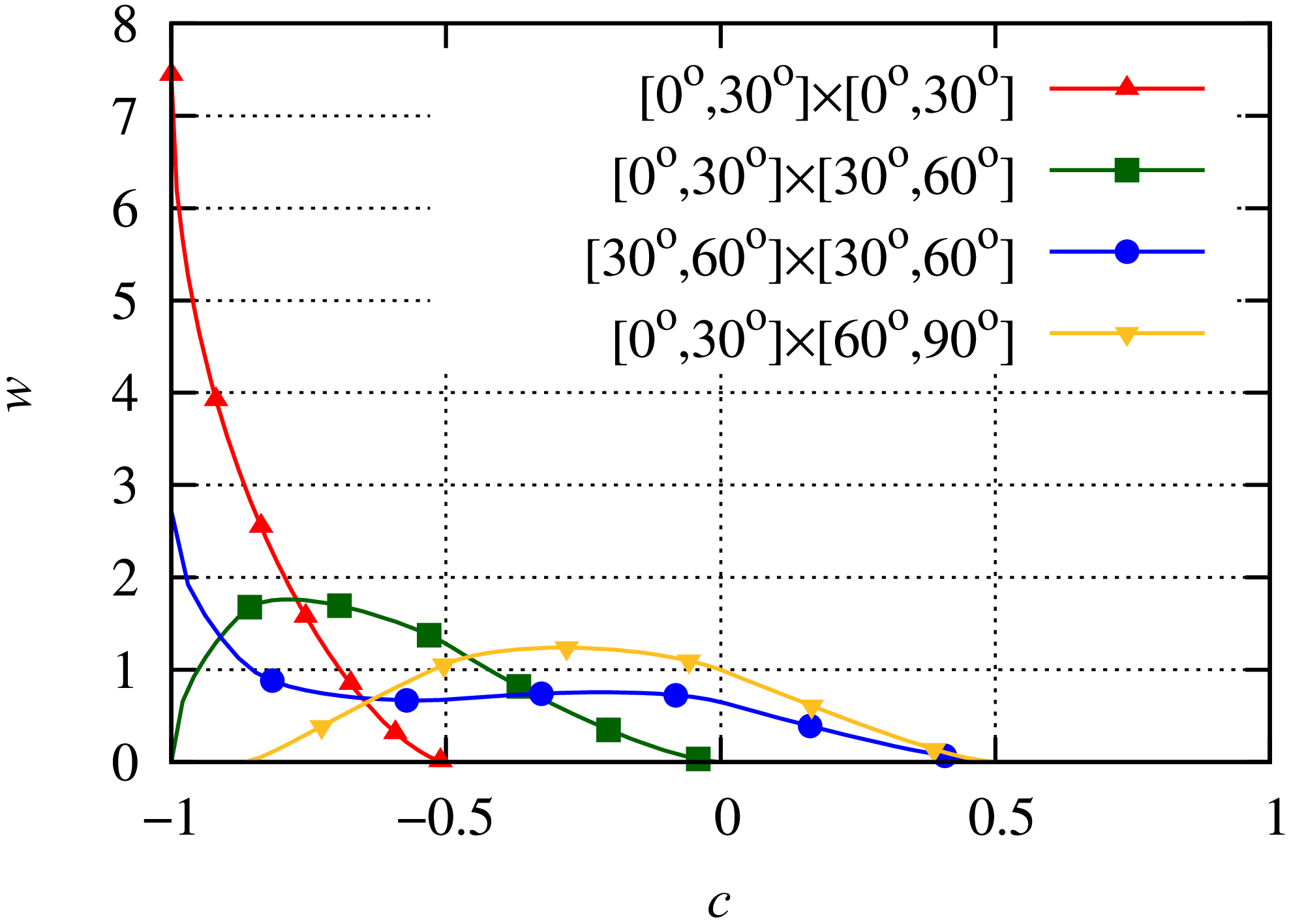The weight function $w(c)$ is independent of energy, non-negative, normalised to unity and sufficiently smooth for practical applications (see figure 1).

Figure 1.

Characteristic form of weighted function. The text box shows the polar angle boundaries of the cells.

Angle averaging reduces to an integration of the weight function over the variable $c$ , simplifying the full averaging defined in (2.3) to

(2.10) \begin{align} R^{a,b}_{i_1,i_2,j_1,j_2} &= \int _{E_{i_1-{({1}/{2})}}}^{E_{i_1+{({1}/{2})}}} \frac { {\rm d}E_a }{ E_{i_1+{({1}/{2})}} - E_{i_1+{({1}/{2})}} } \int _{E_{i_2-{({1}/{2})}}}^{E_{i_2+{({1}/{2})}}} \frac { {\rm d}E_b }{ E_{i_2+{({1}/{2})}} - E_{i_2+{({1}/{2})}} } \nonumber \\ &\quad\times \int {\rm d}c w_{j_1,j_2}(c) R^{a,b}\left ( E_{com} \right )\!,\\[-10pt]\nonumber \end{align}

(2.11) \begin{align} E_{com} &= \frac { m_{ab} }{2} \left ( \frac {E_a}{m_a} + \frac {E_b}{m_b} + 2 \sqrt { \frac {E_a}{m_a} \frac {E_b}{m_b} } c \right )\!, \end{align}

where the reaction rate depends on the centre-of-mass energy $E_{com}$ and $m_{ab} = {m_a m_b}/{(m_a + m_b)}$ is the reduced mass. The numerical evaluation of (2.10) proceeds as follows. The weight function is replaced by piecewise linear approximations. To compute the convolution of $R$ with a linear basis function, two auxiliary integrals are required: $\int ^E R(E) \, {\rm d}E$ and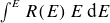 $\int ^E R(E) \, E \, {\rm d}E$ , which are themselves represented using piecewise linear approximations. The discretisation employs $N_w \sim 100$ for the weight function and $N_{rE} \sim 1000$ for the auxiliary integrals (corresponding to an energy step of approximately 1 keV up to an energy of 1 MeV). Evaluation of the inner integral on $c$ in (2.10) is performed via binary search on the tabulated auxiliary integrals with a linear correction, requiring $O(N_w \log _2(N_{rE})$ operations per evaluation. Owing to the smoothness of the energy dependencies, the outer energy integrals in (2.10) were replaced by sum over 3–4 points. Consequently, the complete computation of the $R^{a,b}$ matrix requires $O(N_E^2 N_\theta ^2 10 N_w \log _2(N_{rE})) \sim O(10^4 N_E^2 N_\theta ^2)$ operations, which is computationally tractable. Fusion cross-sections are approximated using the five-parameter formula from Huba (Reference Huba2013).

Table 1.

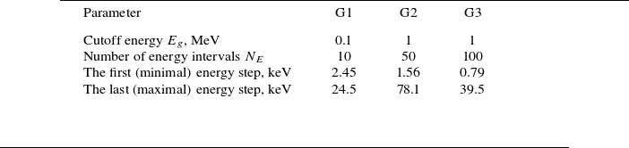
Parameters of grids for figure 2.

Figure 2.

D–T fusion reaction rate (top) and its relative error (bottom) for Maxwellian ions distribution versus ion temperature: DI, direct integration (2.3); G1–G3, calculation on grids by (2.10).

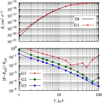
Figure 2 compares the reaction rate for the deuterium–tritium fusion reaction in a Maxwellian plasma, obtained via direct numerical integration of (2.3) (curve DI), with results computed using (2.10) together with piecewise linear approximations on three different grids (curves G1–G3). The grids share two defining features: they span the energy range from 0 to a cutoff energy $E_g$ and their energy steps follow an increasing geometric progression. The parameters of grids G1–G3 are summarised in table 1. Grid G1, which employs only 10 energy intervals, achieves agreement with the direct integration at the 10 % level over the temperature range 0.8–90 keV. The error is largest at low temperatures because the thermal energy becomes comparable to the grid spacing. At the high-temperature end, the discrepancy arises from the finite extent of the grid ( $E_g$ ), which truncates the high-energy tail of the Maxwellian distribution. Increasing both the number of intervals $N_E$ and the cutoff energy $E_g$ systematically reduces the error, as demonstrated by the improved accuracy of grids G2 and G3.

3. Neutral beam capture

The problem of neutral beam capture is decomposed into two components: attenuation of the primary beam and the kinetic evolution of secondary neutrals generated via charge exchange. Both components account for ionisation by electron and ion impact, as well as charge exchange (Bell et al. Reference Bell, Gilbody, Hughes, Kingston and Smith1983; Janev, Reiter & Samm Reference Janev, Reiter and Samm2003).

The interaction of neutral atoms with the plasma is modelled via the continuity equation for the neutral distribution function $g$ :

(3.1) \begin{align} \frac {\partial }{\partial t} g + {\rm div}( \boldsymbol{v} g ) = - \nu ^\varSigma g + G, \end{align}

where $G$ denotes the source term and $\nu ^\varSigma$ is the total charging frequency (i.e. the inverse of the characteristic time for a neutral to get charged). All quantities $g$ , $G$ and $\nu ^\varSigma$ depend on velocity $\boldsymbol{v}$ and coordinates. The charging frequency combines contributions from electron-impact ionisation, ion-impact ionisation and charge exchange:

(3.2) \begin{align} \nu ^\varSigma = \nu ^{es} + \nu ^{is} + \nu ^{cx}, \, \nu ^{is,cx}(\boldsymbol{v}) = \int R^{es,cx}(|\boldsymbol{v}-\boldsymbol{u}|) \, f(\boldsymbol{u}) \, {\rm d}^3 u, \end{align}

with the ion-involved processes given by

(3.3) \begin{align} \nu ^{is,cx}(\boldsymbol{v}) = \int R^{es,cx}(|\boldsymbol{v}-\boldsymbol{u}|) \, f(\boldsymbol{u}) \, {\rm d}^3 u, \end{align}

where $f$ is the ion velocity distribution function. The electron-impact ionisation frequency $\nu ^{es}$ depends solely on the local electron density and temperature, whereas $\nu ^{is}$ and $\nu ^{cx}$ depend on the corresponding reaction rates $R$ and the ion distribution $f$ . The source term $G$ comprises an external component $G^{ext}$ (e.g. the injected beam) and a contribution from charge exchange:

(3.4) \begin{align} G(\boldsymbol{v}) = G^{ext}(\boldsymbol{v}) + f(\boldsymbol{v}) \int R^{cx}(|\boldsymbol{v}-\boldsymbol{u}|) \, g(\boldsymbol{u}) \, {\rm d}^3 u . \end{align}

To resolve the coupling between $G$ and $g$ , the neutral population is decomposed into successive generations: the zeroth generation corresponds to the externally injected beam ( $G^{ext}$ ); the first generation arises from charge exchange between zeroth-generation neutrals and plasma ions; higher generations follow analogously.

The basic MIDAS model operates under two foundational assumptions: axial symmetry and the paraxial approximation. Consequently, axial gradients in plasma parameters are neglected ${\partial }/{\partial z} \approx 0$ . To simplify the velocity–space representation, the coordinate system is rotated about the symmetry axis such that the neutral velocity vector lies entirely in the $x{-}z$ plane, eliminating the $y$ -component of velocity: $\boldsymbol{v} = v_\parallel \boldsymbol{e}_z + v_\perp \boldsymbol{e}_x$ , where $(\boldsymbol{e}_x,\boldsymbol{e}_y,\boldsymbol{e}_z)$ forms an orthonormal basis with $\boldsymbol{e}_z$ aligned parallel to the axis. A steady-state condition is further imposed on the neutral population, rendering the time derivative negligible: ${\partial g}/{\partial t} \approx 0$ . The ion distribution function $f$ is prescribed. Under these constraints, the continuity equation for the $n$ th generation of neutrals reduces to

(3.5) \begin{align} v_\perp \frac {\partial }{\partial x} g^n = - \nu ^\varSigma g^n + G^n . \end{align}

Integration along the characteristic trajectory yields the solution:

(3.6) \begin{align} g^n(x,y,\boldsymbol{v}) & = \int ^{x} G^n(x',y,\boldsymbol{v}) \exp\,[{-}\gamma (x,x',y,\boldsymbol{v}) ] \, \frac {{\rm d}x'}{v_\perp },\\[-10pt]\nonumber \end{align}

(3.7) \begin{align} \gamma (x_2,x_1,y,\boldsymbol{v}) & = \int _{x_1}^{x_2} \nu ^\varSigma (x,y,\boldsymbol{v}) \, \frac {{\rm d}x}{v_\perp } , \end{align}

where $\gamma$ represents the attenuation factor (optical depth) accumulated along the trajectory from $x_1$ to $x_2$ . The local reaction rate density (e.g. ionisation or charge-exchange rate) is then obtained as $\nu ^\varSigma g$ . Finally, the model assumes an isotropic angular distribution of the perpendicular velocity component $v_\perp$ within the transverse $(x,y)$ -plane. Under this condition, angular averaging over the direction of $v_\perp$ is mathematically equivalent to spatial averaging over the $y$ -coordinate.

We now turn to the discretisation scheme employed for numerical calculations. The energy-angle grid defined in (2.1) is adopted for velocity space, as in the preceding section. (Note that distinct grids are preferable for fusion and beam capture problems: ions with energies below 100 eV significantly influence beam capture dynamics, but contribute negligibly to fusion reactivity.) For notational brevity, a single Greek index (e.g. $\alpha$ , $\beta$ ) denotes an individual cell in discretised velocity space. The radial coordinate is additionally discretised into $M$ concentric annular intervals bounded by radii $r_0, \ldots , r_M$ , where $r_0=0$ corresponds to the magnetic axis and $r_M=a$ defines the plasma boundary. Neutrals propagating beyond $r\gt a$ are considered lost from the system. All plasma parameters are assumed constant within each radial interval. The total charging frequency $\nu ^\varSigma$ is evaluated independently for every radial interval $i$ and velocity cell $\alpha$ :

(3.8) \begin{align} \nu ^\varSigma _{i,\alpha } = \nu ^{es}_{i,\alpha } + \nu ^{is}_{i,\alpha } + \nu ^{cx}_{i,\alpha }, \, \nu ^{is,cx}_{i,\alpha } = \sum _\beta R^{es,cx}_{i,\alpha ,\beta } V^v_\beta f_{i,\beta }, \end{align}

where $R_{\alpha ,\beta }$ denotes the reaction rate between neutrals in cell $\alpha$ and ions in cell $\beta$ , respectively, $V^v$ is the velocity–space volume element. The radial index $i$ permits the incorporation of arbitrary radial profiles for plasma parameters. Under these conditions, the fraction of neutrals generated within the $i$ th radial interval that undergo ionisation or charge exchange within the $j$ th interval is given by

(3.9) \begin{align} P^r_{i,j,\alpha } = \int _{O_i} \frac {{\rm d}x \, {\rm d}y}{S_i} \int _{X_j(y)} {\rm d}x' \frac { \nu ^\varSigma _{j,\alpha } }{ v_{\alpha \perp } } \exp [ - \gamma _\alpha (x,x',y) ] H(x'\geqslant x), \end{align}

where $O_i = \{ (x,y) \big | r_{i-1}^2 \leqslant x^2 + y^2 \leqslant r_i^2 \}$ is the source region for interval $i$ , $S_i = \pi ( r_i^2 - r_{i-1}^2 )$ is its area, $X_j(y) = \{ x \big | (x,y) \in O_j \}$ defines the charging region at fixed $y$ and $H$ is the Heaviside step function enforcing forward propagation along the trajectory. Because the attenuation function $\gamma$ of (3.7) is piecewise linear in $x$ , the integrals over $x$ and $x'$ admit closed-form evaluation. To accelerate computation, the curved radial boundaries are approximated by a set of $N_y$ straight lines. High accuracy is retained even for modest $N_y$ ; for instance, $N_y=10$ yields errors below 1 %. Here, $P^r$ is generation-independent. Computing its full set requires $O(N_E N_\theta M^2 N_y)$ operations. The fraction of neutrals escaping radially beyond the plasma boundary is computed analogously to (3.9) by redefining the integration domain for $x'$ to lie outside the plasma.

The charge-exchange probability is defined as the ratio of the charge-exchange contribution in (3.8) to the total charging frequency:

(3.10) \begin{align} P^{cx}_{i,\alpha ,\beta } = R^{cx}_{i,\alpha ,\beta } V^v_\beta f_{i,\beta } \, / \, \nu ^{\varSigma }_{i,\alpha }. \end{align}

The source term for the $n+1$ th neutral generation is computed in two sequential steps:

(3.11) \begin{align} \tilde {G}^{n+1}_{i,\alpha } &= \sum _j P^r_{j,i,\alpha } G^n_{j,\alpha },\\[-18pt]\nonumber \end{align}

(3.12) \begin{align} V^v_{\alpha } G^{n+1}_{i,\alpha } &= \sum _\beta P^{cx}_{i,\beta ,\alpha } \tilde {G}^{n+1}_{i,\beta } V^v_\beta . \end{align}

Here, $\tilde {G}^{n+1}_{i,\alpha }$ represents the total reaction rate density (including both ionisation and charge exchange) for $n$ th generation neutrals undergoing collisions within radial interval $i$ and velocity cell $\alpha$ . The quantity $G^{n+1}_{i,\alpha }$ denotes the source density of $(n+1)$ th generation neutrals produced specifically via charge exchange. Consequently, the ion source density arising from $n$ th generation neutrals is obtained as $\tilde {G}^{n+1}_{i,\alpha } - G^{n+1}_{i,\alpha }$ . Computational complexity per generation is $O(N_E N_\theta M^2)$ for $\tilde {G}^{n+1}$ and $O(N_E^2 N_\theta ^2 M)$ for $G^{n+1}$ and the ion source; the latter typically dominates. Including the precomputation of $P^r$ in (3.9), the total cost scales as $O(N_E^2 N_\theta ^2 M N_g)$ , where $N_g$ is the number of generations retained. The residual fraction of unprocessed neutrals after $N_g$ generations is quantified by $\epsilon _G = \sum _{i,\alpha } G^{N_g}_{i,\alpha } / \sum _{i,\alpha } G^0_{i,\alpha }$ . The value of $N_g$ must be chosen to ensure $\epsilon _G$ falls below a prescribed tolerance. For typical operating parameters of the GDT device (Soldatkina et al. Reference Soldatkina2025), $N_g=10$ generations suffice to achieve $\epsilon _G \lt 1\,\%$ .

The initial source term $\tilde {G}^0$ must be explicitly specified to initiate the iterative procedure. The current implementation models injection of a neutral atomic beam characterised by fixed energy and injection angle relative to the magnetic axis. The beam’s transverse profile is assumed Gaussian:

(3.13) \begin{align} J(y) = \frac {J_0}{\pi y_w} \exp \left ( - \left (\frac {y-y_c}{y_w}\right )^2 \right )\!, \end{align}

where $y_w$ denotes the beam width, $y_c$ the displacement of the beam axis from the magnetic axis and $J_0$ is a beam current in units of particle density per time. Beam attenuation is then computed analogously to (3.9):

(3.14) \begin{align} \tilde {G}^0_{i,\alpha _0} = \int _{-a}^{+a} {\rm d}y \int _{X_i(y)} {\rm d}x \frac { J(y) }{ v_{b\perp } } \exp\, [ - \gamma _{\alpha _0} (-\sqrt {a^2-y^2},x,y ) ], \end{align}

where $v_{b\perp }$ is the beam velocity component perpendicular to the magnetic axis, $\alpha _0$ indexes the velocity–space cell corresponding to the beam parameters on the grid (2.1) and the first argument of $\gamma$ , $-\sqrt {a^2-y^2}$ specifies the plasma entry coordinate at the outer boundary for a given $y$ . As in prior computations, curved radial boundaries are approximated by straight-line segments. Under this approximation – and owing to the piecewise linear form of $\gamma$ – both integrals in (3.14) admit closed-form evaluation in terms of the error function, ensuring high computational efficiency.

We briefly outline the computational algorithm. The procedure begins by computing of the initial neutral source $\tilde {G}^0$ using (3.14), which describes beam attenuation in the plasma. This term contributes positively to the ion source on the right-hand side of the ion kinetic equation (1.1), representing the injected beam capture. This value is included in the output, as beam capture is a measurable quantity in experiments. Subsequently, successive neutral generations are processed iteratively. Each iteration involves two sequential operations. The first is charge-exchange production (3.12): neutrals of generation $n$ are produced via charge exchange. This step contributes negatively to the ion source: $- G^{n}$ . The second step involves computing the total reaction rate of $n+1$ th generation (3.11), accounting for both ionisation and charge exchange. This yields a positive contribution to the ion sources: $\tilde {G}^{n+1}$ . These relationships yield the following inequalities:

(3.15) \begin{align} \sum _{i,\alpha } \tilde {G}^n_{i,\alpha } V^v_{\alpha } \geqslant \sum _{i,\alpha } G^n_{i,\alpha } V^v_{\alpha } \geqslant \sum _{i,\alpha } \tilde {G}^{n+1}_{i,\alpha } V^v_{\alpha }. \end{align}

The neutral population decreases with each iteration due to ionisation (first inequality) and radial escape (second inequality). Consequently, the net ion source is positive, $\sum _{n \geqslant 0} \sum _{i,\alpha } ( \tilde {G}^n_{i,\alpha } - G^n_{i,\alpha } ) \geqslant 0$ , whereas each individual iteration yields a non-positive contribution $\sum _{i,\alpha } ( \tilde {G}^{n+1}_{i,\alpha } - G^n_{i,\alpha } ) \leqslant 0$ . The iterative process terminates after $N_g$ generations. The remaining neutrals, typically few in number, are assigned to either radial loss or capture depending on user settings.

Figure 3.

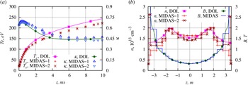
Simulation results for the test configuration: (a) the time dependence of the electron temperature $T_e$ and the beam attenuation coefficient $\kappa$ ; (b) the axial profiles of the plasma density $n$ at time $t=10$ ms and the magnetic field $B$ .

The model has been tested on the next configuration: a 7-m-long device with a mirror ratio of approximately 30 was initially filled with deuterium plasma with a density of a $3 \times 10^{13}$ cm $^{-3}$ and a temperature of 20 eV. An atomic deuterium beam with an energy of 20 keV and a power of 2 MV was injected into the central plane at an angle of $45^\circ$ . The warm plasma density was maintained by a gas puff with a rate of $J_{gas}=300$ eq.A. Three simulation runs were performed: one using DOL code (Yurov, Prikhodko & Tsidulko Reference Yurov, Prikhodko and Tsidulko2016) and two using MIDAS (figure 3). Significant differences exist between the MIDAS and DOL models. DOL separates ions into ‘hot’ and ‘cold’: the fast-ion distribution function is simulated, while the cold-ion density and temperature are estimated using an analytical model. The gas puff is introduced as a source term on the right-hand side of the particle balance equation: $({\partial }/{\partial t}) N_{cold} = \ldots + J_{gas}$ , where $N_{cold}$ is the total number of cold ions throughout the device. Charge exchange with fast ions is neglected for this process. Accordingly, the MIDAS simulations were configured similarly: the gas puff is modelled as a source of low-energy ions with a total current of $J_{gas}$ added to the right-hand side of (1.1). Unlike DOL, however, MIDAS accounts for the axial position of the source. Thus, ‘MIDAS-1’ run places the gas source $J_{gas}$ in the central plane ( $z=0$ ), while ‘MIDAS-2’ distributes $({1}/{2}) J_{gas}$ at two locations near the mirrors ( $z=\pm 3.3$ m). Note that neutral beam capture is modelled through ionisation and charge-exchange processes in both the DOL and MIDAS models. The number of intervals along the $z$ -axis is $N_z=100$ for DOL, compared with $N_z=21$ for MIDAS to accelerate the calculations. Figure 3(a) shows good agreement in beam attenuation and electron temperature, with differences not exceeding 10 %. Thus, the DOL and MIDAS models are consistent. Figure 3(b) shows the axial profiles. The magnetic field profile is similar across all runs. A common feature of the density profiles is the presence of two peaks at $|z|\approx 1.8{-}2$ m, located at the turning points of high-energy ions. However, other features differ as expected. DOL assumes a Boltzmann distribution for cold ions, which becomes inaccurate near the mirrors. In the MIDAS-1 run, low-energy ions are generated in the central plane and are well confined between the turning points. Consequently, the density is higher in the central region and decreases rapidly towards the mirrors. MIDAS-2 assumes generation of low-energy ions near the mirrors, where the electrostatic potential decreases. Two extra peaks appear at these locations, but the low-energy ions are not well confined. As a result, the density is lower in the central region and higher near the ends. Thus, MIDAS yields more realistic profiles than DOL, while the total ion content in the device remains similar across all simulations.

Finally, we discuss the molecular hydrogen gas puff. This can be modelled as a low-energy beam. The majority of neutral particles that penetrate into the main plasma region are so-called Franck–Condon atoms with energies of 6–10 eV. They are produced through ionisation of incoming molecules followed by dissociation in the cold outer plasma layers. It is these atoms that form the low-energy beam. The radial discretisation for the capture problem should be non-uniform, with at least one thin layer at the outer boundary. The thickness of this layer should be comparable to the mean free path of a Franck–Condon atom.

4. Summary

The MIDAS-1D2V model has been extended with two additional modules. The first module calculates fusion reaction rates and can treat charged fusion products as additional ion sources. The second module simulates neutral beam capture, accounting for ionisation by ion and electron impact as well as charge-exchange processes. To date, the implemented physics model includes only hydrogen–isotope interaction processes, but the framework is designed to be extensible should additional reactions be required.