


1. Introduction
When a compliant wall bounds a turbulent flow, the hydrodynamic stresses can lead to deformation of the surface which, in turn, can modify the near-surface flow. This two-way coupling has been the subject of active study due to the potential impact of material compliance on laminar-to-turbulence transition (Metcalfe, Riley & Gad-el Hak Reference Metcalfe, Riley and Gad-el Hak1988), skin friction (Bushnell, Hefner & Ash Reference Bushnell, Hefner and Ash1977) and noise generation (Nisewanger Reference Nisewanger1964). In the present study, direct numerical simulations are performed to examine the two-way interactions between turbulence in channel flow and a viscous hyperelastic wall, with a particular focus on the role of wave propagation in the compliant material.
Early investigations of compliant surfaces were inspired by the potential drag-reducing effects of the skin of dolphins (Kramer Reference Kramer1960, Reference Kramer1962). The original idea was that the compliance damps instabilities and hence can delay breakdown of laminar boundary layers to turbulence. Theoretical studies confirmed the reduction in the growth rate of classical Tollmien–Schlichting waves, and that material damping inhibits flow-induced surface instabilities (Carpenter & Garrad Reference Carpenter and Garrad1985, Reference Carpenter and Garrad1986). These findings were confirmed in experiments (Lee, Fisher & Schwarz Reference Lee, Fisher and Schwarz1993) and direct numerical simulations (Wang, Yeo & Khoo Reference Wang, Yeo and Khoo2006). In a turbulent boundary layer, however, there is no consensus regarding the effectiveness of wall compliance for reducing drag. Various experimental studies were performed, some confirming the reduction in drag (Fisher & Blick Reference Fisher and Blick1966; Choi et al. Reference Choi, Yang, Clayton, Glover, Atlar, Semenov and Kulik1997), and others reporting little change compared with a rigid wall (Lissaman & Harris Reference Lissaman and Harris1969; McMichael, Klebanoff & Mease Reference McMichael, Klebanoff and Mease1980) or even a drag increase (Boggs & Hahn Reference Boggs and Hahn1962) – see Bushnell et al. (Reference Bushnell, Hefner and Ash1977) and Gad-El-Hak (Reference Gad-El-Hak2003) for a comprehensive review.
An important property of compliant materials is their capacity to sustain the propagation of waves whose speed depends on the shear modulus of elasticity of the compliant layer and whose dominant wavelength depends on the layer thickness. Gad-El-Hak, Blackwelder & Riley (Reference Gad-El-Hak, Blackwelder and Riley1984) investigated the spanwise-oriented structures that travel at wave speeds  $U_c$ smaller than $0.05U_0$, where $U_0$ is the free-stream velocity. These static-divergence waves appear when the free-stream velocity exceeds a certain threshold, and are reportedly non-existent in the laminar regime. Duncan, Waxman & Tulin (Reference Duncan, Waxman and Tulin1985) theoretically confirmed the slow propagation of static-divergence waves when $U_0>2.86U_s$, where $U_s\equiv \sqrt {G/\rho _s}$ is the elastic shear-wave speed, $G$ is the shear modulus of elasticity and $\rho _s$ is the density of the compliant material. Travelling wave flutter is another type of instability which travels at an advection speed of approximately $0.7U_0$ (Duncan et al. Reference Duncan, Waxman and Tulin1985; Gad-el Hak Reference Gad-el Hak1986).
Kulik, Poguda & Semenov (Reference Kulik, Poguda and Semenov1991) investigated the frequency band of resonant interactions between turbulent flow and a viscoelastic coating. It was concluded that for a hydrodynamically smooth interaction, the surface deformation must be smaller than the thickness of the viscous sublayer, while for an effective drag reduction the band of the interaction frequencies must be in the region of energy-carrying frequencies. These conclusions hint at simultaneous effects of the wall compliance on stabilizing/destabilizing the flow near the surface. Understanding the nature of these interactions can shed light on the impact of wall properties on turbulence and drag.
More recently, Zhang, Miorini & Katz (Reference Zhang, Miorini and Katz2015) performed tomographic particle image velocimetry of the time-resolved three-dimensional flow in a turbulent boundary layer, and simultaneous Mach–Zehnder interferometry of the two-dimensional deformation at the surface of a compliant wall. In the one-way coupling regime, where surface deformations are smaller than one wall unit, Zhang et al. (Reference Zhang, Wang, Blake and Katz2017) reported two classes of surface motions: (i) a non-advected low-frequency component and (ii) ‘slow’ and ‘fast’ travelling waves with advection speeds approximately  $0.72U_0$ and $U_0$. In addition, the deformation–pressure correlation reached its peak in the logarithmic layer at the same location as the Reynolds shear stress maximum, with the surface deformation lagging the pressure. This streamwise lag was attributed partly to variations of pressure phase with elevations and partly to the material damping. Complementary experiments were performed by Wang, Koley & Katz (Reference Wang, Koley and Katz2020) to investigate the two-way coupling regime where the surface deformation exceeds several wall units. Those authors reported streamwise travelling waves at the fluid–material interface with advection speeds approximately $0.66U_0$, and spanwise waves with an advection speed equal to the material shear speed. The surface deformation, therefore, exhibited a repeated pattern of waves with a preferential spanwise orientation. The most important effects of these waves on the flow were the increase in the near-wall turbulence intensity and a sharp decrease in the streamwise momentum.
Direct numerical simulations were also performed to study drag modification due to compliance. Early investigations modelled the compliant wall as a mass, damper and spring system (Endo & Himeno Reference Endo and Himeno2002; Xu, Rempfer & Lumley Reference Xu, Rempfer and Lumley2003; Kim & Choi Reference Kim and Choi2014; Xia, Huang & Xu Reference Xia, Huang and Xu2017). In this model the wall pressure fluctuations determine the hydrodynamic forcing on the wall; the surface displacement and wall-normal velocity are obtained by solving the spring-and-damper equations and are used as time-evolving boundary conditions to the flow equations. Using this model, Endo & Himeno (Reference Endo and Himeno2002) reported that the in-phase wall velocity and pressure result in a modest drag reduction of approximately  $2.7\,\%$. Xu et al. (Reference Xu, Rempfer and Lumley2003) performed similar simulations, and observed insignificant changes in the near-wall turbulence and drag compared with rigid-wall simulations. They concluded that it is not possible to obtain an in-phase wall velocity and pressure with a uniform compliant wall, and that the drag reduction reported by Endo & Himeno (Reference Endo and Himeno2002) is possibly a transient effect due to the short simulation time. Kim & Choi (Reference Kim and Choi2014) studied softer materials with larger surface deformations. They confirmed the out-of-phase correlation between the wall velocity and pressure, and the drag increase due to the additional form drag on the wall. Those authors also reported large-amplitude quasi-two-dimensional waves propagating in the downstream direction with an advection speed of approximately $0.4U_0$. While the spring-and-damper model has been insightful in understanding some space–time characteristics of compliant walls, it does not account for tangential wall motions which are an important part of wave motion in an elastic layer attached to a rigid wall (Rayleigh Reference Rayleigh1885). In addition, since the vorticity flux at the boundary depends on the tangential acceleration of the surface (Morton Reference Morton1984), neglecting the tangential wall motion is potentially an unjustified simplification.
Rosti & Brandt (Reference Rosti and Brandt2017) performed direct numerical simulations of turbulent flow over a hyperelastic compliant wall in an Eulerian–Eulerian framework, where they employed a volume-of-fluid approach to distinguish the fluid and solid phases. Their approach, thus, accounts for the full wall motion and implicitly satisfies the no-slip boundary condition at the interface. The authors reported a drag increase which is inversely proportional to the rigidity of the compliant material. They discussed a correlation between the wall-normal velocity fluctuations and a downward shift in the logarithmic-layer profile which also becomes steeper. They related their observations to flows over porous media (Breugem, Boersma & Uittenbogaard Reference Breugem, Boersma and Uittenbogaard2006) and discussed them as an extension of flow over rough walls. Within the compliant material, the authors reported that the two-point velocity correlations exhibit oscillating behaviour, and attributed this effect to the typical near-wall flow structures above porous media and rough walls. There was no discussion of wave propagation in the compliant wall.
In addition to the roughness effect of surface undulations, it is important to examine the influence of wave propagation and material acceleration in order to fully characterize the role of wall compliance (Fukagata et al. Reference Fukagata, Kern, Chatelain, Koumoutsakos and Kasagi2008; Józsa et al. Reference Józsa, Balaras, Kashtalyan, Borthwick and Viola2019). The approach adopted herein is inspired by previous analyses of turbulence–wave interaction. This topic of research has a long and rich tradition, starting with the seminal work by Miles (Reference Miles1957, Reference Miles1959) who examined the critical-layer mechanism for the generation of water waves, and followed by a large body of work on the interactions of winds and currents with surface gravity waves (see Sullivan & McWilliams (Reference Sullivan and McWilliams2010) for a review). For instance, the influence of wave kinematics on mean velocity profile, vertical flux of streamwise momentum, Reynolds stresses and surface pressure has been the subject of various studies in air–sea interactions (Sullivan, McWilliams & Moeng Reference Sullivan, McWilliams and Moeng2000; Yang & Shen Reference Yang and Shen2010; Åkervik & Vartdal Reference Åkervik and Vartdal2019; Yousefi, Veron & Buckley Reference Yousefi, Veron and Buckley2020), and their analysis was aided by introducing appropriate surface-fitted coordinates (Hara & Sullivan Reference Hara and Sullivan2015; Yousefi & Veron Reference Yousefi and Veron2020). Similar techniques are adopted herein to examine the implications of wave propagation in a solid material on the adjacent turbulent flow, and conversely the impact of the flow on the surface motion.
In this work, we perform direct numerical simulations of turbulent flow interacting with a neo-Hookean material that satisfies the incompressible Mooney–Rivlin law (Rivlin & Saunders Reference Rivlin and Saunders1997) and compare the results with flow over a rigid wall. The material properties are designed to trigger two-way coupling, and the effects of the Reynolds number, compliant-layer thickness and elastic modulus are examined. The flow configuration, governing equations and computational set-up are described in § 2. The main body of results, including the mean-flow and turbulence modifications, surface spectra and phase-averaged statistics are reported in § 3. Section § 4 contains the discussion and concluding remarks.
2. Methodology
2.1. Problem set-up and governing equations
The flow configuration is a plane channel with one rigid wall and one viscoelastic wall (figure 1), operated at constant mass flux. The nominal half-height of the flow region  $h^\star$ is selected as the reference length, and the bulk flow speed $U_b^\star$ is adopted as the reference velocity; here and throughout, the star symbol indicates dimensional quantities. The streamwise, wall-normal and spanwise coordinates are $\{x, y, z\}$. Undisturbed, the bottom viscoelastic layer occupies $y\in [-L_e, 0]$, and is attached to a rigid backing at $y=-L_e$. The bulk Reynolds number is $\mbox { {Re}} \equiv \rho _f^\star U_b^\star h^\star /\mu ^\star _f$, where $\rho _f^\star$ and $\mu _f^\star$ are the fluid density and dynamic viscosity. The friction Reynolds number is therefore $\mbox { {Re}}_\tau \equiv u_\tau ^\star \mbox { {Re}}/U_b^\star$, where $u_\tau ^\star$ is the friction velocity $u_\tau ^\star \equiv \sqrt {\tau _{w}^\star /\rho _f^\star }$ and $\tau _{{w}}^\star$ is the mean shear stress at $y=0$. In the case of a compliant wall, $\tau _{{w}}^\star$ is comprised of viscous, Reynolds and elastic contributions. When $u_\tau ^\star$ is adopted as the velocity scale, variables are designated by superscript ‘ $+$’. When beneficial to scale variables by the friction velocity from a reference rigid-walls simulation, they will distinguished by superscript ‘ $\ast$’.

Figure 1. Turbulent flow in a channel with a viscoelastic bottom wall. No-slip boundary conditions  $\boldsymbol {u} = 0$ are imposed at $y = \{-L_e, 2\}$, and periodicity is enforced in the $x$ and $z$ directions.
We adopt an Eulerian–Eulerian model to simulate the motion and deformation of the incompressible, viscous, hyperelastic layer interacting with an incompressible flow (Sugiyama et al. Reference Sugiyama, Ii, Takeuchi, Takagi and Matsumoto2011). In order to identify the fluid–solid interface, we employ a conservative level-set approach (Jung & Zaki Reference Jung and Zaki2015; You & Zaki Reference You and Zaki2019). The non-dimensional mass conservation and momentum equations in terms of the velocity field  $\boldsymbol {u}$, pressure $p$ and stress tensor $\boldsymbol {\sigma }$ are unified over the entire domain $\varOmega = \varOmega _f \cup \varOmega _s$:
 $$\begin{gather} \boldsymbol{\nabla}\boldsymbol{\cdot}{\boldsymbol{u}} = 0, \end{gather}$$
 $$\begin{gather}\rho \left( \frac{\partial{\boldsymbol{u}}}{\partial{t}} + \boldsymbol{u} \boldsymbol{\cdot} \boldsymbol{\nabla}{\boldsymbol{u}}\right) ={-}\boldsymbol{\nabla}{p} + \boldsymbol{\nabla}\boldsymbol{\cdot}{\boldsymbol{\sigma}}. \end{gather}$$
The velocity, density and stress fields in the fluid and compliant solid material are denoted by subscripts ‘ $f$’ and ‘ $s$’, and are related to the unified quantities by
 \begin{equation} \boldsymbol{u} = (1-\varGamma)\boldsymbol{u}_s + \varGamma\boldsymbol{u}_f,\quad \rho = (1-\varGamma)\rho_r + {\varGamma},\quad \boldsymbol{\sigma} = (1-\varGamma)\boldsymbol{\sigma}_s + \varGamma\boldsymbol{\sigma}_f, \end{equation}
where  $\varGamma$ is a phase indicator function that is zero in the solid and unity in the fluid phase and $\rho _r\equiv \rho _s^{\star }/\rho _f^{\star }$ is the solid-to-fluid density ratio. The deviatoric components of the stress in the Newtonian fluid and the compliant solid material are
 \begin{equation} \boldsymbol{\sigma}_f = \frac{2}{\mbox{{Re}}} \boldsymbol{\mathsf{D}},\quad \boldsymbol{\sigma}_s = \frac{2\mu_r}{\mbox{{Re}}}\boldsymbol{\mathsf{D}} + {\boldsymbol{\sigma}_e}, \end{equation}
where  $\mu _r\equiv \mu _s^{\star }/\mu ^{\star }_f$ is the ratio between the solid and fluid dynamic viscosities and $\boldsymbol{\mathsf{D}}$ is the strain-rate tensor. In this work, a matching density ( $\rho _r=1$) and dynamic viscosity ( $\mu _r=1$) in the solid and fluid phases are assumed. The former choice is similar to that of earlier studies; for example, Carpenter (Reference Carpenter1998) used comparable densities to achieve flow stabilization by a compliant wall in the transitional regime. And despite that the viscosity ratio in recent experiments was significantly larger than unity (Wang et al. Reference Wang, Koley and Katz2020), our choice of $\mu _r=1$ reduces the material damping and facilitates comparison with recent numerical simulations with the same viscosity ratio at similar Reynolds numbers (Rosti & Brandt Reference Rosti and Brandt2017). The neo-Hookean material is modelled as a particular case of the linear Mooney–Rivlin constitutive equation, and the elastic stress ${\boldsymbol {\sigma }_e}$ is (Rivlin & Saunders Reference Rivlin and Saunders1997)
 \begin{equation} {\boldsymbol{\sigma}_e} = G (\boldsymbol{\mathsf{B}}-\boldsymbol{\mathsf{I}}), \end{equation}
where  $\boldsymbol{\mathsf{B}}$ is the left Cauchy–Green deformation tensor and $G$ and $\boldsymbol{\mathsf{I}}$ are the modulus of transverse elasticity and the unit tensor. Since the upper convective time derivative of $\boldsymbol{\mathsf{B}}$ is identically zero (Bonet & Wood Reference Bonet and Wood1997), a transport equation can be solved to obtain $\boldsymbol{\mathsf{B}}$ in an Eulerian manner (Sugiyama et al. Reference Sugiyama, Ii, Takeuchi, Takagi and Matsumoto2011):
 \begin{equation} \frac{\partial{\boldsymbol{\mathsf{B}}}}{\partial{t}} +\boldsymbol{u} \boldsymbol{\cdot} \boldsymbol{\nabla}{\boldsymbol{\mathsf{B}}} = \boldsymbol{\mathsf{B}} \boldsymbol{\cdot} \boldsymbol{\nabla}{\boldsymbol{u}} + (\boldsymbol{\mathsf{B}} \boldsymbol{\cdot} \boldsymbol{\nabla}{\boldsymbol{u}})^\top. \end{equation}
 A hyperbolic level-set function  $\psi$, which varies sharply from zero to unity across the interface between the compliant wall and the fluid (Desjardins, Moureau & Pitsch Reference Desjardins, Moureau and Pitsch2008), is used to track the interface. The phase indicator is thus $\varGamma = 1$ when $\psi \ge 0.5$ in the fluid phase and $\varGamma = 0$ when $\psi < 0.5$. The transport equation for $\psi$ is
 \begin{equation} \frac{\partial{\psi}}{\partial{t}} + \boldsymbol{\nabla}\boldsymbol{\cdot}{\boldsymbol{u} \psi} = 0. \end{equation}
The hyperbolic level-set function is related to a conventional distance function  $\varphi$ by
 \begin{equation} \psi = \frac{1}{2}\left(\tanh \left(\frac{\varphi}{2\epsilon}\right) + 1\right), \end{equation}
where  $\epsilon \equiv 0.5 \min ({\rm \Delta} x, {\rm \Delta} y, {\rm \Delta} z)$ determines the thickness of the interface marked by $\psi = 0.5$ and ${\rm \Delta} x, {\rm \Delta} y, {\rm \Delta} z$ are the grid sizes in the three physical directions. A reinitialization step is adopted to avoid spurious oscillations at the interface:
 \begin{equation} \frac{\partial{\psi}}{\partial{t'}} + \boldsymbol{\nabla}\boldsymbol{\cdot}{(\psi(1-\psi)\boldsymbol{n})} = \boldsymbol{\nabla}\boldsymbol{\cdot}{(\epsilon (\boldsymbol{\nabla}{\psi}\boldsymbol{\cdot} \boldsymbol{n})\boldsymbol{n})},\end{equation}
where  $t'$ and $\boldsymbol {n}$ are a pseudo-time and the interface normal vector, respectively. The compression term on the left-hand side of (2.9) sharpens the level-set profile across the interface and the diffusion term on the right-hand side imposes a characteristic thickness. Both terms have an inappreciable effect on the interface location, marked by $\psi =0.5$.
No-slip boundary conditions  $\boldsymbol {u} = 0$ are imposed at $y = \{-L_e, 2\}$ and periodicity is enforced in the horizontal $x$ and $z$ directions. Due to the hyperbolic nature of (2.6) and (2.7), they do not require boundary conditions. Continuity of the velocity and traction at the interface implicitly guarantees the no-slip condition, and the interfacial tensions are assumed to be zero at $\psi = 0.5$:
 \begin{equation} \boldsymbol{u}_f = \boldsymbol{u}_s,\quad \boldsymbol{\sigma}_{\boldsymbol{f}} \boldsymbol{\cdot} \boldsymbol{n} = \boldsymbol{\sigma}_{\boldsymbol{s}} \boldsymbol{\cdot} \boldsymbol{n}. \end{equation}
2.2. Material properties and flow conditions
The majority of our discussion focuses on a compliant-wall simulation (case  $C$) that was designed to ensure two-way coupling with the turbulence at $\mbox { {Re}}=2800$. Results are compared with a reference rigid-wall simulation designated $R_{180}$, where the subscript reflects the associated friction Reynolds number. We also examine the impact of the material parameters and the Reynolds number using three additional compliant-wall cases $\{C_G, C_L, C_H\}$ and a rigid-wall simulation $R_{590}$ at a higher bulk Reynolds number $\mbox { {Re}}=10\,935$. In this section, we discuss the design of the simulations and in particular the motivation for our choices of material properties. The case designations and associated physical parameters are summarized in table 1.
Table 1. Case designations and physical parameters of compliant- and rigid-wall simulations.

The design of the main case  $C$ attempts to promote interaction between the surface modes and the turbulent fluctuations. According to linear compliant-material models (Chase Reference Chase1991; Benschop et al. Reference Benschop, Greidanus, Delfos, Westerweel and Breugem2019), uniform pressure fluctuations lead to a peak surface response at wavelength $\lambda _x^\star = 3L_e^\star$ travelling at the free shear-wave speed $u_s^\star = \sqrt {G^\star /\rho _s^\star }$. Based on these estimates, values of $G$ and $L_e$ can be adjusted such that the peak surface mode is excited at a desired pair of streamwise wavenumber and frequency ( $k_x,\omega _t$). For case $C$, we attempt to have this peak ( $k_x,\omega _t$) coincide with the energetic range of the pressure spectra for rigid-wall turbulence:
 $$\begin{gather} E_{pp}(k_x,\omega_t,y) = \langle \hat{p}(k_x,\omega_t,y,z) \times \hat{p}^{\dagger}(k_x,\omega_t,y,z) \rangle_z, \end{gather}$$
 $$\begin{gather}\hat{p}(k_x,\omega_t,y,z) = \int_{-\infty}^{\infty} \int_{-\infty}^{\infty} p(x,t,y,z) \exp({-2{\rm \pi} {\rm i}(k_x x + \omega_t t)})\,\text{d} x\,\text{d} t, \end{gather}$$
where  ${\dagger}$ denotes complex conjugate and $\langle \cdot \rangle _z$ indicates averaging in the $z$ direction. Contours of $E_{pp}$ for the rigid-wall simulation $R_{180}$ at $y^{\ast } \approx 5$ are plotted in figure 2(a). Also shown in the figure is the estimated ( $k_x,\omega _t$) for peak compliant surface response when $G=0.5$ and $L_e=0.5$, which are the parameters for case $C$; the associated wave speed is $u_s=\sqrt {G/\rho _r}=0.71$ and the wavelength is $\lambda _x = 3L_e =1.5$.

Figure 2. Pressure spectra from rigid-wall simulation at  $\mbox { {Re}}=2800$, case $R_{180}$. (a) Wavenumber–frequency power spectra $E^+_{pp}(k_x,\omega _t)$ at $y^+\approx 5$. Marked on the contours are estimates from linear models (Chase Reference Chase1991; Benschop et al. Reference Benschop, Greidanus, Delfos, Westerweel and Breugem2019) for the shear-wave speeds in the designed compliant material $u_s$ (- - -, black) and the peak wavenumber for a given compliant-layer thickness $L_e$ (——, black). (b) Profiles of $\mathcal {E}_{pp}$ as a function of wave speed in viscous (lower axis) and outer (upper axis) units. Shear-wave speeds in the designed compliant material are shown by vertical lines (- - -, red).
Two additional configurations are also marked in the figure, namely cases  $C_L$ and $C_G$, where the dominant wavelength and shear-wave speed are varied independently. In the former, case $C_L$, the compliant-layer thickness $L_e$ is halved compared with case $C$, and in turn the wavenumber of the peak surface mode is doubled (vertical solid lines in figure 2a). For the latter, case $C_G$, the shear modulus of elasticity $G$ is doubled relative to the main case $C$, and therefore the free shear-wave speed is increased to $u_s = 1$ (dashed lines in figure 2a).
The contours of the spectra capture the preferential phase speed  $u_w = k_x/\omega _t$ of pressure fluctuations in the rigid channel, which is important in the context of coupling to propagating waves in the material. In order to highlight this connection, we integrate the pressure power spectra for each $u_\text {w}$ and normalize by the total value:
 \begin{equation} \mathcal{E}_{pp}(u_\text{w},y) = \frac{\displaystyle\int_{-\infty}^{\infty} \int_{-\infty}^{\infty} E_{pp}(k'_x,\omega'_t,y) \delta(\omega'_t / k'_x - u_\text{w})\,\text{d}k'_x\,\text{d}\omega'_t}{\displaystyle\int_{-\infty}^{\infty} \int_{-\infty}^{\infty} E_{pp}(k'_x,\omega'_t,y)\,\text{d}k'_x\,\text{d}\omega'_t}, \end{equation}
where  $\delta$ denotes the Dirac delta function. The resulting $\mathcal {E}_{pp}(u_w)$ is plotted in figure 2(b), evaluated at different heights in the rigid channel. Naturally, the phase speed of the pressure fluctuations increases with height from the wall. What is important to note, however, are the marked shear-wave speeds for cases $\{C, C_L, C_G\}$. All three configurations should be able to couple to the travelling pressure fluctuations in the channel, although the extent of coupling will depend on the amount of energy within specific $(k_x,\omega _t)$ pairs in the coupled simulation; figure 2(a) only provides a rudimentary but informative guide.
For the influence of Reynolds number, we also considered a compliant case  $C_H$ and a corresponding rigid-wall simulation $R_{590}$ at a higher bulk Reynolds number, $\mbox { {Re}}=10\,935$. The wall properties for $C_H$ were selected to match those from the main case $C$, in viscous units. Since the friction velocity is not known a priori, the material design was performed using the friction velocities of the corresponding rigid-wall simulations $R_{180}$ and $R_{590}$ (‘ $\ast$’ variables). The appropriateness of such scaling is discussed in § 3.2, where the compliant-wall responses in cases $C$ and $C_H$ are compared.
2.3. Computational details
The flow equations (2.1) and (2.2) were solved using a fractional-step algorithm on a staggered grid with a local volume-flux formulation (Rosenfeld, Kwak & Vinokur Reference Rosenfeld, Kwak and Vinokur1991; Wang, Wang & Zaki Reference Wang, Wang and Zaki2019). The advection terms were treated explicitly using Adams–Bashforth, and the viscous terms were treated implicitly using the Crank–Nicolson scheme.
The deformation transport equation (2.6) was advanced in time using the low-storage third-order Runge–Kutta scheme. We adopt a special treatment of the advection terms in (2.6), similar to the slope-limiting approach of Vaithianathan et al. (Reference Vaithianathan, Robert, Brasseur and Collins2006). We define a hierarchy of these schemes (centred, upwind-biased, downwind-biased, reduced order) and adopt the first that guarantees a positive definite tensor (for a description, see Appendix B of Hameduddin et al. (Reference Hameduddin, Meneveau, Zaki and Gayme2018)). Adams–Bashforth was adopted for the stretching terms in (2.6). In order to avoid the exponential growth of  $\boldsymbol{\mathsf{B}}$ due to the shearing motion of the fluid, we reinitialize $\boldsymbol{\mathsf{B}}=\boldsymbol{\mathsf{I}}$ in computational cells where $\varGamma = 1$.
For time integration of the level-set transport equation (2.7) and the reinitialization (2.9), we adopt the third-order total variation diminishing Runge–Kutta scheme (Shu & Osher Reference Shu and Osher1989). The advection term in (2.7) was discretized in space using a fifth-order upstream central scheme, while a second-order central differencing was adopted for the compression and diffusion terms in (2.9). The level-set equations were solved in a narrow band around the interface only (Peng et al. Reference Peng, Merriman, Osher, Zhao and Kang1999) to accelerate the computations. Furthermore, (2.9) was invoked every 20 time steps and solved to a steady state in pseudo-time. Following Yap et al. (Reference Yap, Chai, Wong, Toh and Zhang2006), a global mass correction was employed for the level-set function to preserve the initial compliant material mass.
Our numerical method has been extensively validated for studies of transition and turbulence in Newtonian and viscoelastic flows (Lee & Zaki Reference Lee and Zaki2017; Esteghamatian & Zaki Reference Esteghamatian and Zaki2019, Reference Esteghamatian and Zaki2020, Reference Esteghamatian and Zaki2021); the latter feature the upper convective derivative seen in the evolution equation (2.6) for  $\boldsymbol{\mathsf{B}}$. Validation of the interface tracking algorithm was reported by Jung & Zaki (Reference Jung and Zaki2015) who computed the evolution of the Zalesak disc (Zalesak Reference Zalesak1979) and the evolution of linear and nonlinear instability waves in two-fluid flows (Cheung & Zaki Reference Cheung and Zaki2010, Reference Cheung and Zaki2011). In Appendix A, we present an additional validation case to show the accuracy of our two-phase solver in predicting the deformation of a neo-Hookean elastic particle in shear.
Simulation parameters including the Reynolds numbers, domain sizes and grid characteristics are summarized in table 2. The choices of horizontal domain extents,  $L_x$ and $L_z$, were guided by the dominant streamwise and spanwise wavelengths of the surface undulations, and we have verified that these waves are independent of the domain size. For each case, the domain is sufficiently large to accommodate at least eight wavelengths in the streamwise direction and two in the span, and is either equal to or larger than that of previous studies (Shen et al. Reference Shen, Zhang, Yue and Triantafyllou2003; Rosti & Brandt Reference Rosti and Brandt2017). Cartesian grids were adopted with uniform spacing in the streamwise and spanwise directions, and with cosine stretching in the wall-normal coordinate outside the range $-\delta _m \le y \le \delta _m$. The value of $\delta _m$ was selected such that the deformed material surface remains within this range, which is resolved using a fine uniform grid with ${\rm \Delta} y^{\ast } = {\rm \Delta} y^{\ast }_{min}$. The term ‘surface displacement’ is used in reference to the $y$ location of the interface, marked by $\psi =0.5$, relative to the nominal height of the compliant surface $y=0$. The maximum surface displacement $d^{\ast }_{max}$ and the height of the uniform-grid region $\delta _m^{\ast }$ are also reported in wall units, using the friction velocity of the rigid-wall simulations (‘ $\ast$’ variables). We have verified that our results are independent of the grid; for example, in case $C$ we more than doubled the resolution in the streamwise and wall-normal directions and verified that the wall stress and the mean velocity and Reynolds shear stress profiles are unchanged. All simulations were performed with a constant time step ${\rm \Delta} t^\star U^\star _b/ h^\star = \{10^{-3}, 5\times 10^{-4}\}$ for $\mbox { {Re}}=\{2800, 10\,935\}$.
Table 2. Domain size, grid resolution, maximum surface displacement  $d^{\ast }_{max}$ and the height of the uniform grid region $\delta _m^{\ast }$.

The velocity field in the rigid-wall cases was initialized using a superposition of laminar Poiseuille flow and small-amplitude random fluctuations which trigger breakdown to turbulence. Results were only collected after the flow reaches a statistically stationary state. The compliant-wall simulations were initialized with a flat material–fluid interface. The initial velocity field was interpolated from a snapshot of the statistically stationary turbulence over a rigid wall. Here too an initial transient elapsed before statistics were collected for sufficiently long duration in order to ensure convergence, which was verified by comparing results from half and the total number of samples. For example, the statistical sampling period was  $T \equiv t^\star U^\star _b/ h^\star = 550$ convective time units for case $C$, which corresponds to 476 periods of the dominant compliant-material response.
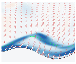
The capacity of a compliant surface to sustain propagating waves is important. In order to examine how quasi-two-dimensional waves interact with the adjacent turbulent flow, we introduce a surface-fitted coordinate system in the  $x$–
$x$– $y$ plane (a detailed description is provided in Appendix B). Figure 3 shows the representation of a velocity vector $\boldsymbol {u}$ in both the original Cartesian and the adopted surface-fitted coordinates. The contravariant components tangent and normal to the surface in this orthogonal curvilinear coordinate system are $u_\xi$ and $v_\eta$, respectively. Phase-averaging was adopted:
 \begin{equation} \varPhi = \bar{\varPhi} + \varPhi'' = \langle \varPhi \rangle + \underbrace{\tilde{\varPhi} + \varPhi''}_{{\equiv} \varPhi'}, \end{equation}
where  $\bar {\varPhi }$ is the phase average and $\varPhi ''$ denotes the pure stochastic term. The second equality is the triple decomposition (Hussain & Reynolds Reference Hussain and Reynolds1970), where $\bar {\varPhi }$ is further decomposed into the average across all phases $\langle \varPhi \rangle$ and the wave-correlated part $\tilde {\varPhi }$. For phase-averaging, crests of streamwise propagating waves $(x_c,d,z_c)$ were identified by satisfying two conditions: (i) the surface displacement $d$ being larger than its instantaneous root-mean-square, $d>d_{rms}$, and (ii) $\partial {d}/\partial {x}$ changing sign.

Figure 3. Schematic of the velocity vector  $\boldsymbol {u}$ in Cartesian coordinates ( $(u,v)$, blue) and in surface-fitted coordinates ( $(u_\xi,v_\eta )$, red).
3. Results
3.1. Global flow modifications
Starting from the Eulerian–Eulerian formulation of the momentum equation (2.2), the mean stress in the streamwise direction can be expressed in terms of the unified field variables:
 \begin{equation} \overbrace{\frac{1}{Re} \frac{\boldsymbol{\text{d}}{\langle u \rangle}}{\text{d}{y}}}^{{\tau_{\mu}}} ~ \overbrace{-\langle u' v' \rangle}^{{\tau_{R}}} + \overbrace{G\langle {(1-\varGamma)}\mathsf{B}_{xy}\rangle }^{{\tau_{e}}} = \left(1 - \frac{y}{2}\right) \tau_{\text{w}} + \frac{y}{2} \tau_{{w,t}}.\end{equation}
From left to right, the total stress is comprised of the viscous contribution  $\tau _\mu$, the turbulent Reynolds stress $\tau _R$ and the elastic term $\tau _e$. On the right-hand side, $\tau _{{w}}$ is the mean shear stress at the nominal height of the compliant surface $y=0$ and $\tau _{{w,t}}$ is the mean stress at the top wall $y=2$. We multiply both sides of (3.1) by $2/h_0$, where $h_0$ is the height at which the total stress changes sign, $h_0=1 + (\tau _{{w}}+\tau _{{w,t}})/(\tau _{{w}}-\tau _{{w,t}})$, and integrate over $0< y< h_0$:
 \begin{equation} \frac{2}{h_0} \int_0^{h_0} \left( \tau_\mu + \tau_R + \tau_e \right)\text{d}y = \tau_{{w}}. \end{equation}
The right-hand side of (3.2) expresses the wall shear stress at the mean location of the compliant surface and the left-hand side shows the contribution of different stress constituents. By normalizing (3.2) with mean wall shear stress in rigid simulation,  $\tau _{{w}}^{\{R_{180},R_{590}\}}$, we can directly compare the contributors to the stress in flow over a compliant surface with that of a rigid wall (figure 4a). Similarly to the recent experimental (Wang et al. Reference Wang, Koley and Katz2020) and numerical (Rosti & Brandt Reference Rosti and Brandt2017) studies, wall compliance increases the drag. The drag increase is associated with an increase in the Reynolds shear stress $\tau _R$, and is largest in the main case $C$. The differences between the stress budgets for cases $R_{180}$ and $C_G$ are within the statistical and discretization uncertainty, which is an indication that the stiffer wall has a minimal impact on the turbulence. The average stresses in (3.1) are evaluated in Cartesian coordinates, and therefore differ from averages performed at locations that are equidistant to the surface. In order to resolve this issue, in § 3.4 we adopt wave-fitted coordinates which also allow us to compute the stress due to the pressure acting on the deformed interface.

Figure 4. (a) Contribution of different stress components to the wall drag (3.1), (3.2). (b) Profiles of the stresses for case  $C$: viscous stress $\tau _\mu$ ( $\cdot \cdot \cdot \cdot \cdot$, black); turbulent Reynolds stress $\tau _{R}$ (- - -, blue); elastic stress $\tau _e$ (——, black); sum of the three components (——, grey). The stresses are plotted in (left axis) outer and (right axis) wall units. (c) Mean streamwise velocity profiles for cases $C$ (——, black), $C_L$ (- $\cdot$- $\cdot$, black), $C_G$ ( $\cdot \cdot \cdot \cdot \cdot$, black), $C_H$ (- - -, black), $R_{180}$ (——, grey) and $R_{590}$ (- - -, grey), compared with experimental data of Wang et al. (Reference Wang, Koley and Katz2020) at $Re_\tau = 5179$ and $G^\star /(\rho _f^\star {U_0^\star }^2)=0.797$ (blue circle). The $y^+$ coordinate is shifted vertically in order to account for the effect of roughness (Jackson Reference Jackson1981).
Note that the drag increase in case  $C_H$ relative to the rigid wall $R_{590}$ is only $5\,\%$, compared with the $46\,\%$ drag increase in case $C$ relative to $R_{180}$. This difference is despite channels $C_H$ and $C$ being designed to have the same amplitude and wavenumber of surface displacement in viscous units. From a roughness perspective, both cases $C_H$ and $C$ belong to a ‘transitionally rough’ regime with $d^+<28$. Therefore, the Reynolds number is expected to influence the normalized drag (Nikuradse Reference Nikuradse1950). A similar trend was observed in the experiments of Wang et al. (Reference Wang, Koley and Katz2020). Those authors reported that the drag increase due to wall compliance relative to a rigid wall reduced from $10.7\,\%$ to $5.0\,\%$ when the Reynolds number was increased by $84\,\%$.
Figure 4(b) shows the stress profiles in case  $C$ where the drag increase is most substantial. Except in case $C_G$ which is almost in the one-way coupling regime, the trends are similar in other compliant cases and therefore are omitted for brevity. The total stress profile, plotted in outer (left axis) and wall (right axis) units, shows the sum of left-hand-side terms in (3.1). The total stress varies linearly with $y$, and its magnitude is larger by approximately $33\,\%$ at $y=0$ than at $y=2$. An important observation is that the Reynolds shear stress changes sign near the surface. This effect is consistently observed in all compliant cases, and is discussed in detail in § 3.4.
Figure 4(c) shows the mean velocity profiles in a semi-logarithmic coordinate in wall units (for completeness, the profiles of the Reynolds normal and shear stresses are provided in Appendix C). For the sake of consistency with the previous literature, the data are first presented in a standard Cartesian coordinate and without any fluid/solid conditional sampling. Since the effective location where the mean drag is exerted on the surface may not coincide with the nominal surface height, in figure 4(c) we use a vertical displacement  $d_h$ proposed by Jackson (Reference Jackson1981) to shift the coordinate. This model is widely used in the study of turbulent flows over rough walls (Leonardi & Castro Reference Leonardi and Castro2010; Ismail, Zaki & Durbin Reference Ismail, Zaki and Durbin2018), permeable walls (Breugem et al. Reference Breugem, Boersma and Uittenbogaard2006) and, more recently, compliant surfaces (Rosti & Brandt Reference Rosti and Brandt2017). The value of $d_h$ is chosen in a way to attain a constant slope in the inertial range, i.e. $(y+d_h)^+ ({{\rm d}\langle u^+ \rangle }/{{{\rm d}y}^+})$ remains approximately constant over the logarithmic layer. The enhanced drag is accompanied by a downward shift in the logarithmic region, even if $d_h=0$. The reduced momentum over compliant material is evident in the shown experimental data of Wang et al. (Reference Wang, Koley and Katz2020) at $\mbox { {Re}}_\tau = 5179$ and $G^\star /(\rho _f^\star {U_0^\star }^2)=0.797$, where $U_0^\star$ is the free-stream velocity. These data were sampled in the flow only and, therefore, are not contaminated by samples within the material; they are also plotted with $d_h=0$.
Unlike the experiments, the computational results are not conditioned on the fluid phase, and hence include samples from the compliant material. In addition, both the experimental and numerical results are plotted in Cartesian coordinates with reference to the nominal interface height, as opposed to the instantaneous interface position. Therefore, averages at a fixed  $y$ location include samples from a range of distances to the surface, which most significantly affects the statistics near the interface. In order to better capture the mean flow in the viscous sublayer, we adopt a surface-fitted coordinate which follows the interface near the compliant surface and smoothly transitions to a Cartesian coordinate with distance from the interface (see Appendix B for details of the surface-fitted coordinates).
Figure 5 shows the mean-velocity profiles compared with the smooth-wall simulations. For cases  $\{C, C_L, C_H\}$, the mean momentum deficit in the logarithmic layer is still observed in the surface-fitted coordinates. The slope of the logarithmic layer, however, does not change significantly, similar to the experimental observations of Wang et al. (Reference Wang, Koley and Katz2020). The viscous sublayer is still retained for the most part, and a decrease in momentum in the buffer layer is observed only in cases $C$ and $C_H$ which, as will be discussed, experience large surface displacements $d^+ \approx 20$. For the stiff material $C_G$, the maximum difference in the profiles from the reference $R_{180}$ case is less than $2\,\%$, which is comparable to the statistical uncertainty (Oliver et al. Reference Oliver, Malaya, Ulerich and Moser2014) and is therefore immaterial – similar to the trends reported by Wang et al. (Reference Wang, Koley and Katz2020) and Rosti & Brandt (Reference Rosti and Brandt2017) for stiff materials; little further attention will be directed to this case.

Figure 5. Mean streamwise velocity profiles in a surface-fitted coordinate: (a)  $C$ (——, black), $C_L$ (- $\cdot$- $\cdot$, black), $C_G$ ( $\cdot \cdot \cdot \cdot \cdot$, black), $R_{180}$ (——, grey); (b) $C_H$ (- - -, black), $R_{590}$ (- - -, grey). The logarithmic law for a smooth wall, $u^+=(1/0.41)\log \eta ^+ + 5.5$, and the viscous sublayer velocity profile, $u^+ = \eta ^+$, are also plotted for reference ( $\cdot \cdot \cdot \cdot \cdot$, blue).
3.2. Deformation and pressure spectra
Visualizations of the instantaneous surface deformation from the compliant wall simulations are shown figure 6. The amplitudes of the displacements are relatively large in cases  $C$ and $C_H$, while the material properties were selected to strongly couple with the turbulence in the channel. Case $C_G$, on the other hand, was designed to have a high material shear-wave speed and, as a result, decouple from the turbulence; this case has the smallest displacements which are of the order of one wall unit. The most salient feature in all cases is the formation of spanwise-oriented surface-displacement patterns that propagate in the streamwise direction. The visualizations also capture a streamwise-oriented pattern with relatively low spanwise wavenumber. The co-presence of the spanwise and streamwise undulations gives rise to a complex topography which is reminiscent of ripples on a water surface. Spanwise-oriented deformation patterns were observed in the experiments of Wang et al. (Reference Wang, Koley and Katz2020), although in their case the surface displacements were more chaotic. Similar to the experiments, the length and width of surface displacements do not vary appreciably with $G$, which is in agreement with the presumption that the peak-wavenumber material response is controlled by the thickness of the layer rather than its modulus of elasticity (Chase Reference Chase1991; Benschop et al. Reference Benschop, Greidanus, Delfos, Westerweel and Breugem2019).

Figure 6. Instantaneous visualization of compliant wall surface, coloured by displacement in wall units, for cases (a)  $C$, (b) $C_L$, (c) $C_G$ and (d) $C_H$.
In order to demonstrate the wave propagation at the material–fluid interface, we examine both the streamwise and spanwise wavenumber–frequency spectra of the surface displacement (figures 7 and 8). In figure 7, streamwise travelling modes are observed in all cases with speeds marginally slower than those of the shear waves in the compliant materials,  $\sqrt {G^\star /\rho _s^\star } = \{0.7, 0.7, 1.0, 0.59\}$ in cases $\{C, C_L, C_G, C_H\}$. As is discussed in § 3.3, the wave motion is very similar to the Rayleigh wave propagating in an elastic material (Rayleigh Reference Rayleigh1885), whose advection speed is similarly slightly smaller than that of the shear wave, i.e. $0.954\sqrt {G^\star /\rho _s^\star }$.

Figure 7. Streamwise wavenumber–frequency spectra of surface deformation for cases (a)  $C$, (b) $C_L$, (c) $C_G$ and (d) $C_H$. Vertical lines indicate the wavenumber corresponding to $3L_e$ and inclined dashed lines indicate different phase speeds.

Figure 8. Spanwise wavenumber–frequency spectra of surface deformation for cases (a)  $C$, (b) $C_L$, (c) $C_G$ and (d) $C_H$. Vertical lines indicate the wavenumber corresponding to $3L_e$ and inclined dashed lines indicate different phase speeds.
In case  $C_G$ with stiff material, the phase speed is relatively high and the resonance is weak, since pressure fluctuations near the wall have lower phase speeds and hence weakly couple to the material deformation. In all cases, the range of dominant wavenumbers are clearly controlled by the material thickness $L_e$, and the peak response shifts to higher wavenumbers in case $C_L$ with the thinner compliant layer (compare figures 7a and 7b). This trend is in qualitative agreement with the predictions by linear models (Chase Reference Chase1991; Benschop et al. Reference Benschop, Greidanus, Delfos, Westerweel and Breugem2019) and the experiments of Wang et al. (Reference Wang, Koley and Katz2020). Relative to the main case $C$, the peak frequencies are higher in cases $C_L$ and $C_G$, the former due to higher range of triggered wavenumbers and the latter due to the larger $u_{w}$.
In the high-Reynolds-number case  $C_H$, the shear-wave speed and layer thickness match with those of case $C$ in wall units. The amplitude and wavenumber–frequency range of excited modes are similar in the two cases, which confirms that selecting the material properties ( $G,L_e$) to be matched in inner scaling was appropriate.
The spanwise wavenumber–frequency spectra (figure 8) do not show clear travelling modes with constant speed. Instead, stationary modes are observed in the spanwise direction, since the pressure fluctuations can trigger spanwise-travelling waves with equal probability of positive and negative velocities. This description is consistent with the time evolution of the surface deformation from the simulations. The frequencies where high energy is observed match the frequencies of the streamwise-travelling waves (compare figures 7 and 8). The interpretation in physical space is one where surface deformations have a nearly standing-wave appearance in the span while they propagate downstream at approximately the shear-wave speed.
The general picture of the spanwise wavenumber–frequency spectra is qualitatively similar to the experimental observations of (Wang et al. Reference Wang, Koley and Katz2020). However, those experiments had reflective lateral boundaries which are inherently different from the periodic ones employed in our simulations. As such, there are some differences, in particular when comparing with their low-fluid-velocity case (equivalent to large non-dimensional  $G$) in which the excited modes were distributed across both low and high frequencies. The authors attributed the energy in the low-frequency range of the spectra to the spanwise-travelling modes, which are only dominant in cases with higher values of $G$. In our simulations, the spanwise waves are mostly stationary, although some weak traces of travelling waves at the shear-wave speed can still be detected, particularly in case $C_H$ (figure 8d). Similar to the experiments, the energy is spread across a range of wavenumbers, and the peak wavelength is smaller than $3L_e$. The peak modes are also at much lower wavenumbers compared with the $k_x$– $\omega _t$ spectra, implying that the surface structures are primarily spanwise oriented.
In order to probe the impact of the travelling surface waves on the flow, streamwise wavenumber–frequency spectra of pressure for case  $C$ are shown in figure 9. The $y^+$ location is selected to be near the interface and beyond the wave crest, in order to avoid sampling the pressure inside the material. For comparison, figure 9(b) shows the spectra for the rigid-wall case at the same Reynolds number and $y^+$ location. The spectra show elevated energy in case $C$ compared with case $R_{180}$. The amplification of pressure spectra is particularly noticeable at advection velocity equal to the Rayleigh wave speed, which is approximately $0.68$ in case $C$; a similar trend was observed for the other compliant cases (not shown). Hence, the modulus of elasticity in wall units can affect both the magnitude and the advection speed of pressure fluctuations near the wall. The amplification of the spectra does not, however, appear to be confined by the wavenumber corresponding to $3L_e$, i.e. the energy is elevated across a wider range of wavenumbers travelling with the same advection speed.

Figure 9. Wavenumber–frequency power spectra of pressure for cases (a)  $C$ and (b) $R_{180}$. The $y^+$ location is above the the crest of surface waves in the compliant case. Vertical lines indicate the wavenumber corresponding to $3L_e$ and inclined dashed lines indicate the bulk velocity $u=1$ and the phase speed of the Rayleigh wave in elastic material, $u_R=0.954\sqrt {G^\star /\rho _s^\star }$.
We interpret the surface deformation through the lens of a response primarily to pressure fluctuations, due to a strong correlation between  $p'$ and $d$ that we report in § 3.3. Note, however, that wave propagation in compliant walls can also be triggered in response to shear-stress fluctuations at the interface (Chase Reference Chase1991; Gad-El-Hak Reference Gad-El-Hak2003). A hint of this effect was recorded in our simulations, where the spanwise shear-stress fluctuations at the surface have a weak correlation with the spanwise undulation of the interface (not shown). In other words, streamwise-aligned near-wall turbulence structures can contribute to the observed spanwise surface undulations in figure 6. Ultimately, since the most prominent effect in our simulations is the streamwise wave propagation, we place our focus on the dominant pressure–deformation interactions.
To identify the pressure disturbances that correlate with the surface deformation, cross-spectra were evaluated in the  $k_x$– $\omega _t$ plane and are plotted in figure 10. The cross-spectra are shown at two different $y^+$ locations for case $C$. In the near-wall region, $y^+=28$, a clear advection band is observed with maximum magnitude coinciding with the peak mode in the surface spectra (compare figure 10a with figure 7a). Below the wavenumber corresponding to $3L_e$, the amplitudes of the cross-spectra reduce and shift to phase speeds closer to the bulk velocity, which correspond to wall signature of larger structures that travel at higher phase speeds. In the logarithmic layer (figure 10b), the overall amplitudes of the cross-spectra diminish, and the peak values are shifted to lower wavenumbers. This trend is expected since relatively larger eddies in the logarithmic layer have a wall signature that can cause deformation of the compliant material.

Figure 10. Pressure–deformation wavenumber–frequency cross-spectra for case  $C$ at (a) $y^+=28$ and (b) $y^+ = 90$. Vertical solid lines indicate the wavenumber corresponding to $3L_e$ and inclined dashed lines indicate the advection velocity of Rayleigh wave in elastic material, $0.954\sqrt {G^\star /\rho _s^\star }$.
3.3. Wave-correlated motions and flow instabilities
So far we have described the wave propagation at the surface of the compliant wall, and its impact on integral flow properties, e.g. drag, mean-flow profiles and pressure spectra. In this section, we closely examine the wave-correlated motions and important features of the pressure and velocity fields in the vicinity of the interface. In doing so, it is helpful to know the velocity field associated with the wave inside the compliant material. Figure 11 shows an instantaneous  $x$–
$x$– $y$ plane with contours of spanwise vorticity near the interface, and the in-plane velocity vectors inside the compliant material. The observed wave motion consists of counter-rotating spanwise rolls, with positive and negative spanwise vorticity below the crest and the trough, respectively. This pattern resembles Rayleigh waves which were first identified at the surface of an isotropic elastic material (Rayleigh Reference Rayleigh1885) and can also be sustained in viscoelastic media (Carcione Reference Carcione1992); they are comprised of vertical and tangential motions that decrease exponentially in amplitude with depth from the surface.

Figure 11. Instantaneous contour plot of spanwise vorticity near the compliant surface and the in-plane velocity vectors inside the compliant wall. Counter-rotating spanwise rolls inside the compliant wall are induced by the Rayleigh wave propagating in the streamwise direction.
We start by evaluating the conditional two-point correlation between the surface displacement and the pressure:
 \begin{equation} R_{dp}({\rm \Delta} x, y, {\rm \Delta} z) = \frac{\langle d(x_0,z_0,t) p(x_0 + {\rm \Delta} x, y, z_0 + {\rm \Delta} z, t) \rangle}{(\langle d(x_0,z_0,t)^2 \rangle\langle p(x_0 + {\rm \Delta} x, y, z_0 + {\rm \Delta} z, t)^2 \rangle)^{1/2}}. \end{equation}
The adopted condition is strong positive displacement, specifically  $d(x_0,z_0,t)>d_{rms}$, and only points in the fluid are sampled. Figure 12 shows $R_{dp}({\rm \Delta} x,y,0)$ for cases $C$ and $C_G$, which feature the largest and smallest surface deformation in wall units. A positive pressure at the surface induces a depression in the compliant material, while a pressure deficit gives rise to a protrusion. Therefore, the displacement is expectedly anti-correlated with the pressure at the surface in both cases $C$ and $C_G$. A phase shift between the displacement and pressure at higher locations is observed, which increases with $y$ and saturates in the logarithmic layer. Zhang et al. (Reference Zhang, Wang, Blake and Katz2017) also reported a phase shift between the near-wall pressure and surface displacement for much stiffer compliant material with surface displacements smaller than one wall unit. In our simulations, the increase in this phase shift with $y$ is more gradual and smooth in case $C_G$ where $d^+_{rms}= 0.55$, while a sharp increase is observed near $y^+\approx 35$ in case $C$ where $d^+_{rms}= 5.6$. Also, while the pressure is minimum at the reference position $(y^+, {\rm \Delta} x)=(d_{rms},0)$ in both cases, a local minimum is observed only in case $C$ at $(y^+,{\rm \Delta} x^+)=(48,41)$. Therefore, it is possible that in case $C$ there are additional unsteady effects due to large surface displacements and strong two-way coupling that lead to a pressure minimum away from the surface. We therefore focus the analysis on this case.

Figure 12. (Top) Spatial correlation between surface displacement and pressure,  $R_{dp}({\rm \Delta} x, y, 0)$, defined in (3.3). Dashed line contours mark negative values, and the positions of minimum value at each $y$ location are indicated by green dots. (Bottom) Phase-averaged surface displacement. All plots are conditioned on strong positive displacement, $d>d_{rms}$. Cases (a) $C$ and (b) $C_G$.
Phase-averaged flow quantities were evaluated for case  $C$ in the surface-fitted coordinate, and are plotted in figure 13. The contravariant wave-correlated velocities, $\tilde {u}_\xi$ and $\tilde {v}_\eta$, are significant near the surface, and penetrate up to $\eta ^+$ locations in the logarithmic layer. Near the surface, the velocity contours are tilted upstream when viewed in the laboratory frame, and are slightly adjusted further away from the wall. In a frame travelling with the wave speed, $\langle u\rangle - u_{w}$ is negative, i.e. the mean flow is in the opposite direction to the wave propagation near the surface; far from the surface the relative flow is positive. The $\eta$ location where the mean velocity matches the wave speed, $\langle u \rangle = u_{w}$, is the critical layer which is marked by a green dashed line in figure 13. Below the critical layer, surface-induced velocity perturbations are advected upstream relative to the wave due to the negative sign of $\langle u\rangle - u_{w}$, which gives rise to velocity contours that are tilted upstream. In contrast, the tilt in the pressure contours is in the forward direction at all heights because it is due to a different mechanism. In congruence with the pressure–deformation correlations (figure 12a), pressure contours away from the surface exhibit a phase lead compared to the pressure at the surface. It is interesting to note that the $\eta ^+$ location of the pressure minimum coincides with the height of the critical layer. One explanation is that unsteady effects in the lee side of the wave, which are further discussed below, give rise to additional turbulent motions and a pressure drop. The positive pressure gradient on the lee side, $0 \le \tilde {x}^+ \le 100$, increases the chance of flow destabilization and shear-layer detachment.

Figure 13. Line and colour contours in surface-fitted coordinates of wave-correlated (a) streamwise and (b) wall-normal contravariant velocities, (c) pressure and (d) surface displacement. In (a–c), negative contour values are plotted with black dashed lines and the green dashed line shows the mean critical-layer height. In (a), the line plot in the right-hand panel shows the mean streamwise velocity in the frame of the wave and averaged over all phases.
Instantaneous flow visualizations in the frame of the wave clarify the unsteady flow features that are not visible in phase-averaged plots. Figure 14 shows a series of snapshots of the vorticity field over a wave crest, which capture the shear-layer detachment near the surface. The vorticity contours are overlaid with line contours of pressure (figure 14a) and velocity vectors in the wave frame (figure 14b). Below the critical layer, where the flow is reversed in this wave frame, the negative vorticity layer on the lee side is lifted up resulting in a significant amount of low-speed fluid being ejected from the wall region. The vertical component of the surface velocity is positive on the lee side (cf. figure 13), which contributes to this lifting process. Once the negative vorticity crosses the critical layer, it is exposed to velocities that are faster than the wave speed, and is detached and transported downstream. The detachment process is reminiscent of a two-dimensional Kelvin–Helmholtz instability and roll-up. The pressure line contours show a drop at the core of the detached vortex, which explains the existence of a pressure minimum in phase-averaged fields (figure 13) at the critical layer downstream of the crest.

Figure 14. Instantaneous visualizations of spanwise vorticity contours in the  $x$–
$x$– $y$ plane over a sample wave crest from case $C$. Colour contour plots are overlaid with (a) line contours of pressure with dashed lines for negative values and (b) velocity vectors in the frame of the wave $(u-u_{w},v)$. Green dashed and solid lines are the instantaneous critical-layer height and the fluid–solid interface, respectively.
Figure 15 shows a three-dimensional view of another instance of this unsteady phenomenon. The isosurface of vorticity coloured by the pressure shows a lifted shear layer which is about to detach. The shape of the layer is locally two-dimensional, which is consistent with the spanwise-aligned rolls formed at the compliant surface. Once the layer is completely detached from the surface, more complex and three-dimensional structures form. This unsteady phenomenon is frequently repeated on the lee side of the wave crest in cases with strong two-way coupling, i.e.  $C$,
$C$,  $C_L$ and $C_H$. Although the instantaneous visualizations show that the lift-up takes place in the lee side, the exact location at which the instability is triggered is not evident from these snapshots. We will investigate the origin of these events, describe the role of surface accelerations and estimate the locations where the velocity profile is most prone to instability.

Figure 15. Instantaneous isosurface of spanwise vorticity,  $\omega _z^+ = 0.275$, coloured by pressure; visualization is from case $C$ and shows a subregion of the domain. The fluid–solid interface is also shown and is displaced vertically for clarity.
The near-interface velocity profile is directly related to the flux of vorticity at the surface. For a solid surface, the ‘vorticity flux density’ is directly related to the tangential pressure gradients (Lighthill Reference Lighthill1963). Morton (Reference Morton1984) extended Lighthill's theory to include the effect of wall acceleration. Since then, active flow control strategies have exploited the relation between vorticity flux, pressure gradient and surface acceleration with the aim of reducing drag (Koumoutsakos Reference Koumoutsakos1999; Zhao, Wu & Luo Reference Zhao, Wu and Luo2004). Since the spanwise vorticity is primarily due to the wall-normal gradient of the streamwise velocity, the vorticity flux at a moving boundary can be approximated by
 \begin{equation} \left.\frac{1}{\mbox{{Re}}}\frac{\partial \omega_z}{\partial \eta}\right\vert_{\eta = 0} \approx \underbrace{\left.-\frac{\partial p }{\partial \xi}\right|_{\eta = 0}}_{S_p} \quad \underbrace{-\frac{\boldsymbol{\text{d}}{u_{s,\xi}}}{\text{d}{t}}}_{S_u}. \end{equation}
The two source terms on the right-hand side are the contributions from the pressure gradient and surface acceleration, where  $\text {d} u_{s,\xi }/\text {d}t$ is the material derivative of the tangential surface velocity. When these terms lead to ${\partial \omega _z}/{\partial \eta }|_{\eta = 0}>0$, the surface is a source of negative vorticity and the velocity profile is stabilized. In contrast, when ${\partial \omega _z}/{\partial \eta }|_{\eta = 0}<0$, the surface is a sink of negative vorticity. As a result, a peak negative vorticity is established near the wall, and the sign of the vorticity gradient changes across it; the location of the peak is therefore an inflection point in the velocity profile.
The sources of vorticity flux were phase-averaged and are plotted in figure 16(a) for case  $C$. The pressure gradient contribution $\overline {S}_p$ is positive (stabilizing) on the windward side and negative (destabilizing) on the lee side of the wave. This picture is consistent with intuition. Interestingly, the surface acceleration source term $\overline {S}_u$ has nearly the same amplitude as $\overline {S}_p$, and is almost out of phase. Due to asymmetries, however, the two contributions do not completely negate each other. The net source term is positive (stabilizing) over the crest and negative (destabilizing) near the troughs. In figure 16(c–f), the profiles of $\overline {\omega _z}^+$ and $\overline {\partial {\omega _z}/\partial {\eta }}^+$ are shown for the phase locations that experience positive (blue) and negative (red) source terms. The blue curves show the enhanced vorticity in the stabilized phases. The red curves show that $\overline {\partial {\omega _z}/\partial {\eta }}^+$ changes sign for a number of phases that are associated with net negative source term, $\overline {S}_p+\overline {S}_u < 0$. While the instabilities are initiated near the troughs where $\overline {S}_p+\overline {S}_u$ is minimum, the lifted shear layer is typically transported backward and towards the lee side of the wave because the local near-interface velocities are negative in the wave frame (cf. figure 14). Also, despite the mean negative values of $\overline {\omega _z}^+$ at the interface, brief instances of $\overline {\omega _z}^+>0$ are common when an instability is triggered, although a complete separation event with flow reversal is extremely rare.

Figure 16. (a) Phase-averaged source terms of vorticity flux (3.4): surface acceleration term  $\overline {S}_u$ (- $\cdot$- $\cdot$, black); pressure gradient term $\overline {S}_p$ (- - -, black); $\overline {S}_u+\overline {S}_p$ (——, black). (b) Phase-averaged surface deformation coloured blue and red for $\overline {S}_u+\overline {S}_p$ positive and negative, respectively. (c–f) Profiles of $\overline {\omega _z}^+$ and $\overline {\partial {\omega _z}/\partial {\eta }}^+$ are conditioned on (c,d) $\overline {S}_u+\overline {S}_p < 0$ and (e, f) $\overline {S}_u+\overline {S}_p > 0$. Dark to light correspond to (c,d) $-20<\tilde {x}^+<40$ and (e, f) $-84<\tilde {x}^+<-20$ and $40<\tilde {x}^+<84$.
We now direct our focus to the impact of wall properties and Reynolds number on the competing effects of pressure gradient and surface acceleration (figure 17). In both cases  $C_L$ and $C_G$, the two sources of vorticity flux remain out of phase. However, the pressure source is larger, and the net term $\overline {S}_p+\overline {S}_u$ is mostly negative (stabilizing) in the windward side of the wave and vice versa. Note that in these two compliant cases the surface displacements, and in turn the surface accelerations, are small in wall units relative to the main case $C$. Therefore, the compliant walls for cases $C_L$ and $C_G$ approach the behaviour of rigid roughness where the pressure gradient contribution is the only source of vorticity flux. In the case with higher Reynolds number $C_H$, the net source term and individual contributions are similar to those of case $C$. The wave amplitude in wall units, which is almost equal in cases $C$ and $C_H$, is therefore a controlling parameter in the balance between $\overline {S}_p$ and $\overline {S}_u$.

Figure 17. Similar to figure 16(a,b), except for cases (a,b)  $C_L$, (c,d) $C_G$ and (e, f) $C_H$.
3.4. Form drag, pressure work and near-wall stresses
In this section we examine the impact of the compliant wall on the flux of streamwise momentum in the surface-normal direction and the energy exchange with the flow. Due to the surface deformation, form drag becomes relevant. While the impact of form drag is unambiguous in rough walls (Jiménez Reference Jiménez2004), studies of air flow over surface gravity waves suggest a more nuanced role, e.g. form drag can reverse sign and drive the wind for fast waves (Gent Reference Gent1977; Sullivan et al. Reference Sullivan, McWilliams and Moeng2000).
The phase-averaged pressure  $\overline {p}^+$ and form drag $\overline {p \partial d /\partial x}^+$ for case $C$ are shown in figure 18(a). As discussed in § 3.3, the pressure is out of phase with the surface displacements. There is an asymmetry in the pressure relative to the wave crest, and the minimum pressure is slightly shifted towards the lee side of the wave. The pressure drag onto the surface $\overline {p \partial d /\partial x}^+$ (figure 18b) is also asymmetric relative to the crest. The net effect is a positive drag on the interface, which is most pronounced in case $C$ (see also table 3). In cases with smaller surface displacements (not shown), such as $C_G$, not only is the wave-correlated pressure smaller, but also the pressure is more symmetric with respect to the crest. Both effects result in a reduced form drag.

Figure 18. Phase-averaged surface quantities in case  $C$. (a) Pressure $\overline {p}^+$ (——, black) and surface-normal velocity $\overline {v_{s,\eta }}^+$ (- - -, green), (b) form drag $\overline {p\partial {d}/\partial {x}}^+$ and (c) pressure work exerted by the fluid onto the surface $\overline {-p v_{s,\eta }}^+$. Surface displacement is schematically marked in the bottom of each panel.
Table 3. Space- and time-averaged pressure work exerted by the fluid onto the surface  $\langle -p v_{s,\eta } \rangle ^+$, form drag $\langle p \partial {d}/\partial {x}\rangle ^+$ and surface shear stress $-\langle u'_s v'_{s,\eta } \rangle ^+$.

Unlike for a rigid wall, the fluid can exert pressure work onto the compliant material,  $\langle -p v_{s,\eta } \rangle ^+$, where $v_{s,\eta }$ denotes the interface-normal velocity. The phase-averaged $\overline {v}^+_{s,\eta }$ is included in figure 18(a) along with the pressure. The surface motion is downward on the windward side and upward on the lee side of the wave, and lags the pressure by a phase shift of nearly ${\rm \pi} /2$. The correlation is plotted in figure 18(c), and inherits the asymmetry of the pressure ( $\overline {v}_{s,\eta }^+$ will be shown to closely match the symmetry of Rayleigh waves; cf. figure19). Again, the net effect integrated over the entire surface is positive in all cases (table 3). Therefore, the fluid exerts work on the compliant material and this energy exchange is primarily due to the vertical motion of the wave.

Figure 19. Phase-averaged surface quantities in case  $C$. (a) Surface velocities in streamwise $\tilde {u}^+_s$ (——, blue) and surface-normal $\tilde {v}^+_{s,\eta }$ (——, red) directions. (b) Phase-averaged wave-induced shear stress $-\tilde {u}^+_s\tilde {v}^+_{s,\eta }$ (——, black). Velocities and stresses are also plotted from solution of the Rayleigh wave equations: horizontal velocity $u_R^+$ (- - -, blue), vertical velocity (- - -, red) and shear stress $-u_R^+v_R^+$ (- - -, black). Surface displacement is schematically marked in the bottom of each panel.
In § 3.1 we showed that the Reynolds shear stress, evaluated in Cartesian coordinates, changes sign near the surface and is negative at  $y=0$. This effect is revisited here in more detail, using wave-fitted coordinates and phase averaging. We recall that Rayleigh waves at the free surface of an elastic material have zero shear stress because its sinusoidal horizontal and vertical velocities are ${\rm \pi} /2$ out of phase. Therefore, in our configuration the turbulent flow alters the surface wave motion in a manner that gives rise to finite net shear stress. We plot our phase-averaged interface velocities and the surface motion of classical Rayleigh waves in figure 19; the comparison is qualitative and only intended to contrast the relative phases of the two velocity components. It is clear that $\tilde {v}^+_{s,\eta }$ is essentially sinusoidal, while $\tilde {u}^+_s$ deviates from the Rayleigh wave motion in particular on the lee side. This deviation is due to the reaction force of the fluid onto the surface, in response to the total drag. As is discussed below, turbulent and pressure drag are particularly large in the lee side of the wave near $0<\tilde {x}^+<50$. The reaction force on the material is, therefore, also large and in the positive $x$ direction, which decreases the magnitude of the negative tangential velocity of the surface in that $\tilde {x}^+$ range. Ultimately, $-\tilde {u}^+_s\tilde {v}^+_{s,\eta }$ also deviates from the Rayleigh sinusoidal pattern, with the largest difference on the lee side. Consistent with our earlier observations in Cartesian coordinates (§ 3.1), $-\langle u'_s v'_{s,\eta } \rangle ^+$ averaged over the entire surface is negative in all cases (table 3).
The extent to which the negative shear stress at the surface persists into the flow is examined in figure 20. We report the phase-averaged shear and pressure stresses in surface-fitted coordinates. We only present case  $C$ because the results are qualitatively similar for cases $C_L$ and $C_H$, and the wave-correlated stresses are negligible for case $C_G$. The contours of the wave-correlated component of the Reynolds shear stress $- \tilde {u}\tilde {v}_\eta$ reflect the importance of the critical layer and the wave boundary-layer height (figure 20a). The latter is defined as $h_\text {w} \equiv \sqrt {\nu \lambda _x /u_{w}}$, where $\lambda _x$ is the dominant streamwise wavelength and is approximately $h_{w}^+ \approx 4$. Below this height the motion of the fluid is appreciably influenced by the wave, and hence the patterns of $- \tilde {u}^+\tilde {v}_\eta ^+$ are very similar to those reported at the surface (compare with 19b); the net contribution $\langle - \tilde {u}\tilde {v}_\eta \rangle ^+$ is therefore negative. Between $h_{w}^+\approx 4$ and the critical-layer height, the negative stress decays and the positive stress increases substantially, resulting in a change of sign of the net contribution, $\langle - \tilde {u}\tilde {v}_\eta \rangle ^+$. The flow below the critical layer, which spans the viscous sublayer and part of the buffer layer, is simultaneously influenced by the wave motion and the turbulence. Above the critical layer, the magnitude of $- \tilde {u}\tilde {v}_\eta$ decays quickly and is practically negligible. As such, the critical-layer height demarcates the region of impact of the wave-correlated stresses above the surface, similar to turbulent air flow above gravity waves (Sullivan et al. Reference Sullivan, McWilliams and Moeng2000; Yousefi et al. Reference Yousefi, Veron and Buckley2020).

Figure 20. Phase-averaged stresses in surface-fitted coordinates for case  $C$. (a) Wave-correlated $- (\tilde {u}\tilde {v}_\eta )^+$ stress, (b) stochastic Reynolds shear stress $- \overline {u'' v''_\eta }^+$ and (c) pressure stress $-\overline {(p/J) \partial \eta /\partial x}^+$ and phase-averaged surface displacement $\overline {d}^+$. The line plots in the right-hand panels show the quantities averaged over one wavelength. The horizontal lines show the height of the wave boundary layer ( $\cdot \cdot \cdot \cdot \cdot$, black) and the height of the critical layer (- - -, black).
The stochastic turbulent stresses  $- \overline {u'' v''_\eta }^+$ are shown in figure 20(b). Except for the region below $h_{w}$ on the windward side of the wave, $- \overline {u'' v''_\eta }^+$ is positive everywhere. The stresses peak between the trough and the critical layer, where the unsteady shear-layer detachment events described in § 3.3 are most probable. Above the critical layer, the patterns of strong positive $-\overline {u'' v''_\eta }^+$ are tilted forward due the higher local velocities.
The wave-correlated and stochastic components of the Reynolds stresses are interdependent. For example, the production of the latter includes  $P_{ij} = -\langle \overline {u_i'' u_k''} \partial \tilde {u}_j/\partial {x_k} + \overline {u_j'' u_k''} \partial \tilde {u}_i/\partial {x_k} \rangle$, which involves the wave-correlated velocity gradient. This term represents the production of small-scale turbulence energy in phase with the wave (Barbano et al. Reference Barbano, Brogno, Tampieri and Di Sabatino2022), and the same term appears with an opposite sign in the equation of the wave-correlated stresses. An in-depth analysis of the energy exchange between the mean flow, wave-correlated velocities and stochastic fluctuations is left to future research.
The pressure stress  $-\overline {(p/J) \partial \eta /\partial x}^+$, where $J$ is the Jacobian of the coordinate transformation, is shown in figure 20(c). Below the wave boundary layer, the pressure drag is equal to the form drag at the surface, and alternates between negative and positive stress on the windward and lee sides of the wave. Above the wave boundary layer, however, only positive drag is observed. This positive pressure stress has a phase lead above $h_{w}$, and is due to the unsteady shear-layer detachment events that take place on the trough. Note that the pressure stress by definition depends on the curvature of the isolevels of $\eta$, and therefore it gradually decays to zero as the impact of surface undulations diminishes away from the surface. The pressure itself, however, remains correlated with the wave at much higher $\eta$ locations, as previously seen in figure 13(c).
3.5. Three-dimensional effects
Since the propagating waves in the compliant layer are primarily spanwise-oriented rolls, we have so far focused on a two-dimensional analysis of the wave-correlated velocities. However, as shown previously in spanwise wavenumber–frequency spectra (figure 8), finite  $k_z$ deformations are present although at lower wavenumbers compared with the streamwise ones. In this section we investigate the impact of three-dimensionality of the surface on the wave-correlated velocities and Reynolds shear stress.
We start by analysing the surface velocities associated with the wave propagation (figure 21). Despite the interface undulation in the span, the surface-velocity vectors are mostly two-dimensional and dominated by their  $x$ and $y$ components. These two components are associated with the streamwise-propagating rolls, which dominate the surface motion. The spanwise interface velocity (colour contours) is smaller in magnitude, and has a wave-correlated pattern: the sign of $\overline {w}_s$ matches that of $\overline {v}_{s,\eta }\overline {n}_z$, where $\overline {n}_z$ is the spanwise component of the surface-normal vector. The observed pattern is better understood considering the combined effects of streamwise wave propagation and spanwise surface deformation. At $\tilde {z}=0$, the wave propagation is sustained by upward velocities on the lee side giving way to downward velocity on the windward side of the crest (vector plots in figure 21). In the region ( $0<|\tilde {z}|<|\lambda _z/2|$), where $\lambda _z$ is the dominant spanwise wavelength, the interface-normal velocity has a component in the spanwise direction. The product of $\overline {v}_{s,\eta }$ and $\overline {n}_z$ determines the sign and magnitude of $\overline {w}_s$. Due to the phase relation between $\overline {v}_{s,\eta }$ and $\overline {n}_z$, the maximum amplitude of $\overline {w}_s$ occurs at $\tilde {z} = \pm \lambda _z/4$. Physically, the interface on the lee side is stretched outward in the span as it is pulled away from the wall, and on the windward side it is squeezed in the span towards the middle as it retracts towards the wall. While these three-dimensional features of the surface are more clearly observed in cases $C_L$ and $C_H$, similar patterns are also observed in cases $C$ and $C_G$ (not shown). In case $C$, the spanwise-oriented rolls are dominant and hence the structures are less three-dimensional. In case $C_G$, the wave-correlated velocities are in general smaller due to the weaker coupling between surface and flow.

Figure 21. Phase-averaged surface displacement, velocity vectors and contours of the spanwise component of surface velocity near the crest. Cases (a)  $C_L$ and (b) $C_H$. The surface displacement is multiplied by a factor of two for clarity.
Figure 22 shows phase-averaged quantities below and above the surface for case  $C_L$. The phase-averaged pressure isosurfaces are shown in figure 22(b). They are predominantly two-dimensional, echo the wave motion in the streamwise direction and their magnitude is largest in the span above the crest. The vertical velocity component inside the compliant layer and in the fluid is clearly dominated by the wave motion (figures 22c and 22d). The spanwise fluid velocity $\bar {w}$ in figure 22(e) matches the above description of figure 21; the velocity structures are, however, asymmetric in the direction of wave propagation, specifically stronger on the windward side of the wave. This asymmetry is due to the presence of a secondary flow which we discuss below. The streamwise velocity fluctuations with respect to the Cartesian average $\overline {u}^+-\langle u\rangle ^+$ are shown in figure 22( f). While influenced by the interface wave motion in the streamwise direction, there is also a clear spanwise dependence due to the three-dimensionality of the interface. Specifically, the streamwise velocity is slower above the spanwise crests and faster above the spanwise troughs. Momentum transport across this spanwise gradient, $-\bar {w}{\partial \bar {u}}/{\partial z}$, can contribute to drag (Jelly, Jung & Zaki Reference Jelly, Jung and Zaki2014). In particular, on the windward side of the travelling wave where the magnitude of $\bar {w}$ is larger, the term $-\bar {w}{\partial \bar {u}}/{\partial z}$ is positive and, therefore, a drag penalty.

Figure 22. Phase-averaged isosurfaces from case  $C_L$. (a) Fluid–solid interface, (b) pressure $\bar {p}$, (c) wall-normal velocity inside the compliant wall $\overline {v_s}^+$, (d) wall-normal velocity in the fluid $\overline {v}^+$, (e) spanwise velocity $\bar {w}$ and ( f) streamwise velocity fluctuations $\overline {u}^+-\langle u\rangle ^+$.
The three-dimensionality of the flow is further examined by plotting phase-averaged fields in cross-flow planes on the windward (figure 23a,b) and lee (figure 23c–f) sides of the wave. Of particular interest is the phase-averaged streamwise vorticity which can capture secondary flows that may arise due to inhomogeneity in near-wall turbulence (Perkins Reference Perkins1970). For compliant walls, an additional source of streamwise vorticity is the spatial variation in surface velocity, specifically  $\partial \overline {v}_{s,\eta } / \partial {\zeta }$, where $\zeta$ is the unit-tangent vector to the surface in the cross-flow plane. In the figure, vectors show the in-plane components of the phase-averaged flow velocity. Since the range of magnitudes differs appreciably near to and away from the interface, the vector fields are plotted twice, with vector lengths proportional to the velocity magnitudes in figures 23(a) and 23(c), and using uniform vector lengths in figures 23(b) and 23(d). On the windward side, strong patterns of $\overline {\omega _x}$ with opposite signs are observed at the surface, which are primarily generated due to the gradient of wall-normal surface velocities, $\partial \overline {v}_{s,\eta } / \partial {\zeta }$ (figure 23a). The sign of this near-surface vorticity is reversed on the lee side, again due to the surface motion. We focus our attention on the weaker pattern of $\overline {\omega _x}$ that is observed away from the surface, which does not reverse direction from the windward to the lee side. The uniform vector fields show an associated pair of counter-rotating streamwise vortices whose cores coincide with the local extrema of $\overline {\omega _x}$, and whose core-to-core spacing is roughly half the dominant wavelength of the spanwise surface undulations.

Figure 23. Phase-averaged contours of (a–d) streamwise vorticity  $\overline {\omega _x}^+$, (e) streamwise velocity $\overline {u}^+$ and ( f) $\overline {u''w''}^+$. Vectors are in-plane phase-averaged velocity $(\overline {w}^+,\overline {v}^+)$. Vector lengths in (a,c) are scaled by the magnitude of the in-plane velocity and in (b,d) are uniform. The streamwise locations are (a,b) in the windward side, $\tilde {x}^+ = -17$, and (c–f) in the lee side, $\tilde {x}^+=17$, of the streamwise wave.
The outer vortex motion is best characterized as Prandtl's secondary flows of the second kind, and is comparable to those observed above streamwise-aligned riblets (Goldstein & Tuan Reference Goldstein and Tuan1998) and superhydrophobic textures (Jelly et al. Reference Jelly, Jung and Zaki2014). It is generated due to the inhomogeneity in Reynolds stresses in the span. In particular,  $\partial ^2 \overline {w''w''} /\partial {y} \partial {z}$ is the dominant source term in the streamwise vorticity equation, and changes sign across the spanwise crest. The pair of counter-rotating vorticies are therefore generated by the turbulence above the spanwise surface undulation, and are largely independent of the streamwise phase: the secondary-flow vorticies away from the surface are similar in figures 23(b) and 23(d).
With the above description in mind, it is helpful to recall the pattern of the spanwise surface velocities (figure 22e). The stronger  $\bar {w}$ on the windward side arises because the spanwise motion of the surface (figure 21a) has the same sign as the spanwise velocity of the outer secondary vortex near $\tilde {y}^+ \approx 25$. In contrast, on the lee side of the wave, there is a reversal in the spanwise wall velocity alone while the outer secondary flow remains unchanged. As a result, their superposition leads to a weaker $\bar {w}$.
Another implication of the spanwise surface undulations is the generation of a stochastic Reynolds stress  $\overline {u''w''}$ (figure 23f). Patterns of positive and negative $\overline {u''w''}$ on both sides of the crest are visible, and arise due to turbulence production against the spanwise shear, $-\overline {w''w''}\partial \bar {u}/\partial {z}$ (figures 23f and 23e). A fluid parcel which is transported by a stochastic perturbation from the crest towards the positive $z$ direction ( $w''>0$) carries low-momentum fluid towards the high-momentum zone ( $u''<0$). This and the opposite motion results in $\overline {u''w''}<0$. Conversely, $\overline {u''w''}>0$ is generated on the other side of the crest. The spanwise gradient of $\overline {u''w''}$ is therefore negative near $\tilde {z} = 0$, implying that the lateral turbulent transport above the crest results in a drag penalty. This effect, however, is expected to be cancelled by the negative drag contribution over the spanwise troughs where ${\partial \overline {u''w''}}/{\partial z}>0$.
These results highlight the central role of the propagation of quasi-two-dimensional surface waves in studying the interaction of turbulence with a compliant surface. In addition to the roughness effect and the incurred form drag, the surface velocities modify the flow structures near the interface and up to the logarithmic layer, contribute to the flux of vorticity at the interface and give rise to energy exchange between the flow and the surface. While the surface waves are spanwise-elongated, they also express low-wavenumber spanwise undulations. The three-dimensionality of the wave motion generates streamwise vorticity near the interface and a secondary outer flow with an associated spanwise inhomogeneity.
4. Summary and conclusions
The interaction of channel-flow turbulence with a compliant wall was examined using direct numerical simulations in an Eulerian–Eulerian framework. The compliant layer was an incompressible viscous hyperelastic material. We considered layers with different thicknesses and elastic shear moduli, selected based on the response of compliant coatings in one-dimensional linear models (Chase Reference Chase1991; Benschop et al. Reference Benschop, Greidanus, Delfos, Westerweel and Breugem2019), and also considered two Reynolds numbers. Consistent with the recent experimental (Wang et al. Reference Wang, Koley and Katz2020) and numerical (Rosti & Brandt Reference Rosti and Brandt2017) efforts, we observed enhanced turbulence intensity, which resulted in reduced streamwise momentum and a drag increase. We showed that, in a surface-fitted coordinate, the wall compliance gives rise to a downward shift of the logarithmic layer without a significant impact on the viscous sublayer. Spanwise-elongated deformations of the surface propagated as waves in the streamwise direction, and their impact on the flow was investigated through the lens of wave–turbulence interactions.
The surface deformation spectra showed a band of streamwise-advected waves with phase speed equal to that of Rayleigh waves. The range of energetic wavenumbers was shifted to higher values in the case with a thinner layer, and the stiffer compliant material sustained higher wave speeds. The design of the higher-Reynolds-number case aimed at constant values of  $G^+$ and $L_e^+$, which led to similar spectra thus demonstrating the relevance of the viscous scaling for the material parameters. In the spanwise direction, most of the surface energy was concentrated at low wavenumbers without a clear indication of spanwise-travelling modes. The range of excited frequencies in $k_z$– $\omega _t$ spectra coincided with that in $k_x$– $\omega _t$ spectra, which supports the view that the streamwise travelling waves set the frequency response. It is of note that spanwise wave propagation was also occasionally observed in the time series of the flow field, but much less discernible than the downstream propagating counterpart. The evolution of the surface directly impacted the pressure field, which was captured in the pressure spectra and the deformation–pressure cross-spectra.
The travelling Rayleigh waves in the compliant material were comprised of out-of-phase wall-normal and streamwise velocities whose influence penetrates deep into the flow. Visualizations of the instantaneous vorticity field in the frame of the wave showed frequent shear-layer detachment that was initiated near the trough. The detached layer rolled up near the critical layer (where the flow speed is equal to the Rayleigh wave speed) accompanied by a local pressure drop. The origin of these detachment events was studied by evaluating two sources of spanwise-vorticity flux at the surface: the pressure gradient and a nearly out-of-phase surface acceleration due to the Rayleigh waves. For small-amplitude waves, the pressure gradient term was dominant and, similar to static roughness, was favourable on the windward side and adverse on the less side. For large-amplitude waves, the contribution by surface acceleration became significant, and the stabilized flow region shifted towards the lee side of the wave.
The fluid exerted a net positive pressure work onto the solid surface. The asymmetry of pressure with respect to the crest of the waves resulted in form drag that opposed the near-wall streamwise momentum. The Rayleigh waves were also affected by the flow, in particular their streamwise velocity component. As a result, the compliant material sustained a negative wave-correlated Reynolds shear stress. This wave-correlated shear stress rapidly changed sign above the wave boundary layer and below the critical layer. The stochastic shear stress was also substantial in this region due to the unsteady shear-layer detachment events.
While the surface waves were primarily two-dimensional, the surface also exhibited low-wavenumber spanwise undulations. The associated phase-averaged flows were examined. The streamwise velocity was relatively slow above the spanwise peaks and fast above the spanwise troughs. Strong streamwise vorticity was generated by the surface motion, specifically the spanwise gradient of the surface-normal velocity. The pair of opposite-sign vorticity on the windward side reversed sign on the lee side of the wave. Away from the surface, counter-rotating vortices signalled the presence of a secondary flow. In addition, the spanwise gradient of the mean streamwise velocity led to the generation of stochastic  $u''w''$ stresses. All these flow features in turn modified the wall-normal and lateral transport of momentum and, in turn, drag.
On the other hand, we also showed that the surface acceleration contributed a spanwise vorticity flux which is out of phase with respect to the pressure gradient along the surface topography. This flux can potentially be harnessed to stabilize the flow and mitigate the unsteady detachment of near-wall vorticity. Finally, the herein discussed results can guide future studies and designs of compliant coatings for turbulent flow applications, and may motivate new innovative designs, for example that exploit anisotropic material properties to suppress or promote particular effects.
Funding
This work was supported in part by the Office of Naval Research (grant N00014-20-1-2778). Computational resources were provided by the Maryland Advanced Research Computing Center (MARCC).
Declaration of interests
The authors report no conflict of interest.
Appendix A. Validation of the numerical algorithm
The level-set algorithm for capturing the material–fluid interface was extensively validated (Jung & Zaki Reference Jung and Zaki2015). An additional validation case is presented here, where the deformation of a neo-Hookean elastic particle subjected to a simple shear flow is simulated and compared with data of Villone et al. (Reference Villone, Greco, Hulsen and Maffettone2014).
An initially spherical neo-Hookean elastic particle with undeformed radius  $r_0^\star$ is placed at the centre of a cubical domain. The ratio between the undeformed radius of the particle and the wall-normal height of the domain $H^\star$ is $r_0^\star /H^\star =0.1$. The flow is induced by two parallel plates located at $y^\star = \{-H^\star /2, H^\star /2\}$, moving opposite to one another in the $x$ direction with the same speed, generating a constant shear rate $\dot {\gamma ^\star }$. Periodicity is imposed in $x$ and $z$ directions, and the isotropic homogeneous grid resolution is set to ${\rm \Delta} x^\star = r_0^\star /24$.
The particle deforms due to the applied shear flow, until it reaches a steady-state ellipsoid-like shape. The Reynolds number is sufficiently small to avoid inertial effects ( $\mbox { {Re}}_{r} \equiv {r_0^\star }^2\dot {\gamma ^\star }/\nu ^\star = 0.025$), and three different elastic capillary numbers $Ca \equiv \mu ^\star \dot {\gamma ^\star }/G^\star = \{0.05, 0.2, 0.35\}$ are simulated for comparison with data of Villone et al. (Reference Villone, Greco, Hulsen and Maffettone2014). As shown in figure 24, agreement between the reference data and our numerical predictions in particle deformation is satisfactory. We have also successfully reproduced the migration trajectories of elastic particles reported by Villone et al. (Reference Villone, Greco, Hulsen and Maffettone2014) (their figure 5, not shown). These tests validated our treatment of the elastic material–fluid interface, in both steady and time-dependent problems.

Figure 24. Shape of a deformed neo-Hookean particle in a Newtonian fluid under confined shear flow for (a)  $Ca=0.05$, (b) $Ca=0.2$ and (c) $Ca=0.35$. The fluid–solid interface is projected onto the plane of shear located at $z=0$, and the axes are normalized by the undeformed radius of the particle. Present simulations (solid blue line) are compared with the data of Villone et al. (Reference Villone, Greco, Hulsen and Maffettone2014) (square symbols).
Appendix B. Surface-fitted coordinates
Surface-fitted coordinates are introduced in order to probe the wave-induced motions near the interface. We define a coordinate system that follows the interface near the compliant surface and smoothly transitions to laboratory Cartesian coordinates away from the surface. Such a coordinate system is particularly of interest for horizontal averaging, were the  $y$ location of data points in a Cartesian coordinate is not an accurate measure of the distance to the surface. The adopted coordinate transformation is widely used in analysis of experimental measurements above ocean waves (Hara & Sullivan Reference Hara and Sullivan2015; Yousefi & Veron Reference Yousefi and Veron2020).
Following Benjamin (Reference Benjamin1959), the surface displacement at each spanwise location is first decomposed into corresponding spatial Fourier components, i.e.  $d(x) = \varSigma _n a_n\exp (i(k_n x + \phi _n))$, where $a_n$, $k_n$ and $\phi _n$ are amplitude, wavenumber and phase of the $n$th mode. The orthogonal coordinates $(\xi,\eta )$ are defined by
 $$\begin{gather} \xi = x - {\rm i}\varSigma_n a_n\exp ({\rm i} (k_n x + \phi_n)) \exp({-}k_n {y}), \end{gather}$$
 $$\begin{gather}\eta = y -\varSigma_n a_n\exp ({\rm i} (k_n x + \phi_n)) \exp({-}k_n {y}). \end{gather}$$
Appendix C. Fluid-conditioned Reynolds stresses
Profiles of Reynolds normal and shear stresses conditioned on the fluid phase are plotted in Cartesian coordinates in figure 25. All quantities are normalized by wall units, and  $\langle \varGamma \rangle >0.5$ is satisfied at all $y$ locations in order to ensure a sufficient number of statistical samples.

Figure 25. Different components of the Reynolds stress tensor conditioned to the fluid phase: (a–c)  $C$ (——, black), $C_L$ (- $\cdot$- $\cdot$, black), $C_G$ ( $\cdot \cdot \cdot \cdot \cdot$, black), $R_{180}$ (——, grey); (d–f) $C_H$ (- - -, black), $R_{590}$ (- - -, grey).
As remarked in the main text, case  $C_G$ which is in the one-way coupled regime has minimal effect on the turbulence statistics relative to the reference case $R_{180}$. For all the other complaint-wall configurations, $\langle u'^+_f u'^+_f \rangle$ and $\langle v'^+_f v'^+_f\rangle$ increase sharply near the wall, which highlights the strong impact of the wave motion on the near-wall turbulence. Wall-normal fluctuations peak at $y^+=0$, while $\langle u'_f u'_f\rangle$ reaches its maximum near the bottom of the buffer layer. These trends are most pronounced in cases $C$ and $C_H$, where the surface displacements are relatively large in wall units, and the wave impact is significant up to the buffer layer. The impact of wall compliance on $-\langle u'^+_f v'^+_f \rangle$ is weaker relative to the normal stresses, similar to the trends observed in the experiments of Wang et al. (Reference Wang, Koley and Katz2020).


 Open access