




1. Introduction
The study of long-run living standards lies at the very core of economic history and development research, and price history is one of its most essential building blocks. Pre-modern price indices, key deflators in establishing the real value of consumption and incomes, are dominated by the cost of foodstuffs, which is reasonably well documented for a wide variety of global locations. The cost of shelter, arguably as important a factor as food for human well-being, is much less well-understood, especially over periods spanning several centuries. Omitting the expenditure on housing, or, as is more common, assuming an arbitrary weight for it in consumption budgets, risks introducing biases of unknown direction and magnitude into the measurement of living standards, as well as distorting international comparisons.Footnote 1 Incorporating time- and quality-consistent series of housing costs into the construction of long-run consumption baskets is therefore essential for understanding the evolution of economic well-being, both in absolute terms and in comparative settings.
This paper builds on Drelichman and González Agudo’s (Reference Drelichman and González Agudo2014) study of Toledo’s housing market between 1489 and 1650, extending the series of rental costs to 1810, exploring its response to various social, political, and economic events, and proposing measures suitable for inclusion in estimates of living standards. The result is one of the longest series of rents available for any period and location in the pre-modern world.
Assembling a long-run series of housing costs is fraught with challenges. Using house ownership records as a source has been all but impracticable. Central land registries were not introduced in most countries until the late nineteenth or early twentieth century. Notarial protocols documenting real estate transactions are extremely unwieldy sources, disorganized and scattered in the best of cases, or altogether missing. Even when it is possible to obtain and clean transaction data with a reasonable effort, extracting the value of housing services over the long run from infrequent purchasing transactions poses a whole new set of theoretical and empirical difficulties. Consequently, there are very few pre-modern studies on the cost of house ownership over the long run.
The standard approach to computing the value of housing services with modern-day data is to control for quality by studying repeat purchases of the same property. The only example of a very long-run index built with this methodology is Eichholtz (Reference Eichholtz1997), whose database is structured on the basis of repeat purchases of houses on the Herengracht canal of Amsterdam between the seventeenth and the twentieth centuries. Clark (Reference Clark2002) and Raff et al. (Reference Raff, Wachter and Yan2013) also observe purchase data, though not necessarily of the same properties over time, in their long-term studies of London and Beijing real estate. Despite the high quality of these databases, extracting the annual value of housing services from them remains a challenge, especially in light of the fact that they tend to capture very wealthy parts of the market. A related approach involving the use of fiscal valuations is employed by Steensel et al. (Reference Steensel, van Oosten and Hooymans2025) in their study of housing wealth in Leiden.
The more common strategy to study pre-modern housing costs has been to build a series of rental rates, an approach that has recently been expanding in both coverage and quality as more archival records from large landlords are brought to light. Series for various periods built with diverse methodologies exist for Amsterdam (Lesger, Reference Lesger1986), Antwerp (Scholliers, Reference Scholliers1962), Brussels (Avondts, Reference Avondts1971), Bruges (Mason, Reference Mason and Verlinden1959), Ghent (Van Ryssel, Reference Van Ryssel1967), London (Ormrod et al., Reference Ormrod, Gibson and Lyne2011), Milan (Barbot and Percoco, Reference Barbot, Percoco, Canepari and Crisci2019), Madrid (Llopis and García Montero, Reference Llopis and García Montero2011), Toledo (Drelichman and González Agudo, Reference Drelichman and González Agudo2014), and Edirne (Karagedikli and Coşkun Tunçer, Reference Karagedikli and Coşkun Tunçer2021). A comparative analysis of seven European cities is offered by Eichholtz et al. (Reference Eichholtz, Korevaar and Lindenthal2025).
Rent-based series, in principle, provide a more straightforward window into the value of housing services, but also come with their own challenges. Ensuring representativeness is the first hurdle; sources that span very long periods can be peculiar in their own right, and so can their real estate holdings. Next comes the need to define consistent units of analysis across time and space. Quite often, the units rented are not described in detail. It is difficult to infer the hedonic characteristics of something described only as a “house” and to ascertain whether unit size or quality changes as time passes. Long-term leases, which in several pre-modern settings could span several lifetimes, must be evaluated in light of inflationary expectations. The pricing mechanisms used by the landlord need to reflect market prices, or at least be consistent with profit maximization, requiring the economic historian to gain deep institutional knowledge of the practices of the property owner. And, finally, in order to interpret the long-run dynamics in the data, it is important to have a thorough understanding of the broader socioeconomic context.
Toledo presents several desirable characteristics for the study of long-run rents. Unlike Madrid, its economic and real estate markets were not distorted by the large footprint of the Royal Court and its wealthy entourage. Having lost most of its political influence in the mid-sixteenth century, the city’s fortunes were typical of those of a regional administrative center. Its long-term population dynamics are reasonably well documented. While the study of its economic activity and development has been patchier, enough sources exist to compose a reasonable panorama. Finally, its perch atop a circular hill surrounded by the river Tagus on three sides makes it an almost ideal incarnation of the monocentric city model.Footnote 2
Drelichman and González Agudo’s (Reference Drelichman and González Agudo2014) series is anchored in a detailed inventory of the holdings of the Cathedral of Toledo dating back to 1489. Their analysis stopped in 1650, owing to the increasingly distant connection to the inventory and the consequent thinning out of the sample. In the absence of a similar document for the later period, we adopt a different methodological approach, trading off individual detail for representativeness. Instead of collecting the rents paid for a dwindling smattering of properties with known hedonic characteristics, we captured every single rental unit in the Cathedral’s portfolio. The resulting dataset contains as much as 35% of all urban dwellings in each sampled year, assuaging any concerns that may arise from the lack of positive identification of each unit. It also represents a tenfold increase in the annual average number of observations, forcing us to forgo annual samples in favor of decadal ones. In Section 3, we explore the implications of this methodological break and establish the conditions under which we can splice the two datasets.
Our combined data allow us to study rental costs between 1489 and 1810 for a wide variety of subsamples and cross-sections. In Section 4, we study the rates paid for entire residential properties, analyzing them by type of residence, location, intended use, renter socioeconomic status, and gender. In Section 5, we further refine the analysis to produce estimates of individual housing costs, which are suitable for inclusion in the construction of price indices, personal budgets, and estimates of living standards such as welfare ratios.
Our series sheds light on several relationships between macroeconomic shocks and housing costs. All the rents for entire properties show a large increase in the 1550–1575 period, matching the Dutch disease episode triggered by the arrival of large quantities of Peruvian silver in Spain (Drelichman, Reference Drelichman2005). When examining the rents paid for individual living spaces, however, a stark contrast arises between the privileged classes and the working poor. The former, to whom much of American wealth accrued, furiously bid up rents in the central neighborhoods of the city, which rose by almost 300% and took on bubble-like characteristics. In outlying neighborhoods, rents paid by the working poor increased by just under 60%. This result highlights the inequality in the variation of disposable income at the different ends of the socioeconomic spectrum as a result of an exogenous shock.
A second salient result is the increase in both nominal and real rents in the aftermath of the monetary stabilizations of 1680 and 1720. Both episodes resulted in strong deflation for staple goods, but rent moved in the opposite direction. This is consistent with housing acting as a residual item on personal budgets, absorbing whatever disposable income was available after satisfying the food requirements of a family. Stabilizations brought predictability to both goods and labor markets, with the prices of staple goods falling faster than wages. In a context of inelastic supply of housing, the resulting real disposable income was absorbed by urban rents.
A final stylized fact is that, despite the very high housing costs observed at the heyday of the sixteenth century, and the temporary boosts to the market provided by monetary shocks, by 1810 all measures of rents had fallen to approximately 50% of their 1490s levels in real terms. The long-run profile of the series mirrors the inexorable urban decline of Toledo. The progressive reorientation of economic activity toward Madrid, a series of epidemics starting in the 1590s, the ill-conceived municipal fiscal policy in the second quarter of the sixteenth century, and a marked loss of population sparked a process of urban decline that proved irreversible.Footnote 3 Feeble attempts at creating an industrial sector via chartered monopolies did little for the health of the urban economy. As the Cathedral struggled to find tenants for its vast holdings of real estate, the once proud City of Kings became one of many sleepy provincial capitals, its low rents reflecting the weak purchasing power of its inhabitants and the lack of desirability of its once prized housing stock.
2. Historical and institutional background
Owing to its privileged position at a crossroads near the geographical center of the Iberian peninsula, Toledo was an urban nexus of paramount importance since antiquity. After its reconquest by Christian armies in 1085, it grew steadily in both political and ecclesiastical influence. The itinerant Royal Court chose it as its residence for extended periods, thus promoting the construction of luxurious lodgings and the establishment of supply chains for all sorts of foodstuffs and manufactured goods. As early as 1088, the Diocese of Toledo was designated as a Primatial See by the Pope, endowing it with the political backing to exert its influence over the entire Spanish church and to increase its material possessions over time.Footnote 4
As part of Castile’s demographic expansion in the first half of the sixteenth century, Toledo’s population grew to nearly 50,000 inhabitants, making it the second-largest city in Spain after Seville.Footnote 5 Its economic life was underpinned by a vibrant textile industry, which reached its peak in the early sixteenth century; after a period of crisis preceding and following the revolt of the Comunidades, it caught a second wind fueled by exports to the colonies in America.Footnote 6 Toledo’s ascendancy continued even when, in 1561, Philip II settled the royal court in Madrid, starting a process that would, in time, reduce the city’s political and ecclesiastical influence.Footnote 7 Mineral wealth from the Americas found its way to Toledo, where it funded monumental buildings and timeless works of art. It also fueled a frenzy at the top end of the real estate market, with those in positions of privilege bidding up rental rates for prestigious properties to extremely high levels. Rents eventually came down with the end of the silver-induced Dutch disease in the 1570s. Though the period was punctuated by the occasional subsistence crisis, the city nevertheless continued to benefit from a strong manufacturing and trading sectors, as well as to sustain a population in the neighborhood of 50,000 inhabitants, well into the 1590s.
The turn of the seventeenth century brought much bleaker tidings for Toledo. The Atlantic plague of 1599 decimated its population, the chronic military and fiscal struggles of the Crown resulted in an increase in fiscal pressure, and the growth of Madrid began to attract skilled workers away from the city. The ensuing population drop sparked a vicious cycle as the authorities tried to compensate for the revenue shortfalls by increasing local taxes, which only served to accelerate the exodus. By the middle of the seventeenth century, Toledo’s population was about half its 1570s peak levels.Footnote 8 The situation continued to worsen until the 1680s, when the effects of the monetary reform and a variety of epidemics delivered the most punishing crisis the city had yet experienced.Footnote 9 Population remained stagnant at historically low levels until the end of the War of the Spanish Succession in 1715, after which it slowly recovered to reach between 15,000 and 18,000 inhabitants in the late eighteenth and early nineteenth centuries.Footnote 10
In the seventeenth and eighteenth centuries, Toledo became almost exclusively defined by the presence and influence of the Catholic Church. At the time of the Ensenada Cadastre (1751–1753) there was one nun or friar for every eight lay inhabitants, while ecclesiastical institutions received upwards of 80% of all land rents and owned up to 70% of houses inhabited by private individuals.Footnote 11 Part of the fiscal troubles of the city can arguably be traced to the Church’s tax exemptions and its effective blocking of fiscal reform.Footnote 12
The eighteenth century saw renewed attempts to revitalize the city’s industry and commerce through the establishment of Royal companies, most saliently in its historically strong sectors of silk and sword production. The Royal Company of Manufacturing and Commerce, chartered in 1748, managed to sustain up to 250 silk looms for about a decade before slowly declining until its disappearance in the 1780s. The Royal Weapons Factory had few spillovers. At the same time, the learned societies on economic matters that characterized the Spanish Enlightenment failed to gain more than a toehold in Toledo, where they were under the stifling control of the ecclesiastical authorities.Footnote 13
Early modern ecclesiastical institutions were typically endowed with a variety of income streams to support their operations. For those located in urban settings, such as major Cathedrals, rental houses, and shops featured prominently among their sources of revenue. Their legal status as “dead hands” meant that they generally could not sell or otherwise dispose of property, while acquisitions and donations progressively added to their holdings. By the beginning of the sixteenth century, the Cathedral Chapter of Toledo had accumulated 557 urban properties, almost certainly making it the largest landowner in the city.Footnote 14 The day-to-day management of this portfolio fell to an office by the name of Refitor, which was charged with renting out each property for as much as it would fetch, as well as with overseeing their upkeep.Footnote 15 Its annual record of rental transactions, called the Carta Cuenta, is the main source of our data.
The Refitor used several contractual forms to lease out its properties. In the late Middle Ages, the predominant arrangement was the perpetual lease, called censo or tributo perpetuo. Under this type of covenant, the use of the property was ceded in perpetuity to the leaseholder and his or her descendants for a fixed annual payment. The lease could be transferred to another person only with the explicit approval of the Refitor, which it normally granted in exchange for a transfer fee of 10% of the sale price, called alicer. Although the Cathedral Chapter retained eminent ownership, it could only repossess a property leased in perpetuity in case of default in payments, unapproved sale, or abandonment. Because the annual payments were fixed in nominal terms, periods of inflation significantly eroded their value. By the late fifteenth century, the Cathedral Chapter had stopped entering into perpetual leases, but existing ones remained on the books for as long as their conditions were met, often well into the seventeenth and eighteenth centuries.
In the sixteenth and early seventeenth centuries, virtually all new rental contracts took the form of long-term leases. Their annual payment was still fixed for the duration, but the contract expired after a set number of “lives.” In the case of one-life leases, the property returned to the Cathedral Chapter after the death of the leaseholder. Under two- and three-lives leases, the contract expired after all of the original leaseholder and either one or two designated successors died. Designated successors were always family members, and could not be more than one generation younger than the leaseholder. Three-lives leases, for example, were typically granted to a man, his wife, and one son or daughter.
When a property became available to lease, the Refitor decided whether to offer it under a one-, two-, or three-lives lease, and announced a two-week viewing period. Leases were then adjudicated at a public auction, which ensures that we are observing market prices. Long-term leases could, by their very nature, last for several decades. In order to set a reservation price, the Refitor had to take into account the impact of inflation on a potentially long contract, as did the aspiring leaseholders, in order to make their bids. Uniquely, the prices of long-term leases were expressed as a combination of cash and live hens, with the latter providing a partial inflation shelter. When expressed entirely in monetary amounts, two- and three-lives lease payments were respectively 25% and 40% higher than those for a single-life lease.Footnote 16
The second and third quarters of the seventeenth century were a period of heightened monetary upheaval. The issuance of copper fiat currency, first introduced in the late 1590s, accelerated sharply after the end of the Twelve Years’ Truce in 1621. Prices fluctuated wildly as ineffective stabilization attempts, devaluations, and revaluations followed each other in rapid succession. The instability came to an end with the currency reform of the 1680s.Footnote 17 By then, the contractual landscape in the rental market had been fundamentally reshaped.
During the sixteenth century, when the Refitor could not obtain its reservation price at an auction for a long-term lease, it would rent the property for a period of a few months to a year in an all-cash contract, thus buying itself some time before trying again for a better auction result. These short-term rentals, called alquiles, became increasingly common in the second quarter of the seventeenth century, as the urban decline of Toledo and the increasing inflation uncertainty made both landlords and renters wary of committing to nominal long-term contracts. By 1650, short-term rentals had become the norm. Their length was standardized at a year for urban properties and three years for rural ones, and their name changed to the modern term alquileres. At some point between 1650 and 1660, the Refitor stopped recording payments for existing long-term leases in the Carta Cuenta; they were likely moved to a different set of books that have not been located. All new rental agreements from then on took the form of annual cash leases.
The transition to short-term leases also brought about a second change in the structure of the rental market. Under the long-term leasing regime, the Refitor only rented out entire houses. The average built area of residential properties in the Drelichman and González Agudo (Reference Drelichman and González Agudo2014) dataset was 261 square meters, reflecting buildings suitable for housing several families. The leaseholders of the larger properties would often act as middlemen, subletting portions to several other individuals or families. The change to annual rental contracts, which started and ended at different times of the year, made such an intermediation structure impractical. When it could not rent out an entire house, the Refitor partitioned the properties itself, directly renting individual rooms, sets of rooms, coach houses, and a host of other spaces to different individuals. In Section 5, we exploit this trait to identify the size of living spaces and construct long-term measures of individual housing costs.
3. Data and dataset compatibility
The new data collected for this paper consists of every rental agreement in the Carta Cuenta in years ending in zero between 1650 and 1810. For each entry, we record the type of property (or fraction thereof), the neighborhood or parish, the annual rent paid (pro-rated as necessary), the gender of the tenant, whether the tenant used any academic or honorific titles (such as Doctor, Licenciado, Don or Doña), the number of tenants, and their occupations. For women, we also record whether they were never married, married, or widowed. Each of the 17 sampled years featured between 463 and 694 transactions, for a total of 10,631 observations.
The nature of the data in the post-1650 period required a collection methodology that resulted in some significant differences with the dataset in Drelichman and González Agudo (Reference Drelichman and González Agudo2014) for 1489–1650. We first describe how our data differs from theirs, and then explain how we combine the two datasets to create series that can encompass the entire period.
Drelichman and González Agudo (Reference Drelichman and González Agudo2014) dataset (hereafter “DGA”) contains all the properties owned by the Cathedral that satisfied two conditions: they were archaeologically identified and described by Passini (Reference Passini2004), and they could be linked between an inventory conducted by the Cathedral Chapter in 1491 and the Carta Cuenta. The advantage of this approach is that the 1491 inventory yielded a rich set of hedonic characteristics for each property. These included the built area, the number and nature of internal spaces, and the presence of amenities such as water wells or facilities for keeping animals. The archaeological identification made it possible to precisely geolocate each property on a street map. Since the DGA dataset recorded tenant and payment data for every year, it also made it possible to track individual properties through time. For all of its advantages, however, the DGA dataset suffers from two main drawbacks. First, selecting properties on the basis of modern-day archaeological identification introduced survival bias, which skewed the dataset toward higher-quality houses in wealthy neighborhoods.Footnote 18 Second, the anchoring to the 1491 inventory meant that properties that dropped out of the sample, usually because of redevelopment or an unrecorded tenancy change, could not be replaced. By 1650, only 113 properties remained in the sample, of which just 66 were not subject to perpetual leases (and can hence yield useful information to establish rental costs). Beyond that point, the shrinking sample size and attendant loss of representativeness more than outweighs the advantages of precise geolocation or hedonic characterization.
Since we do not have an inventory with which to meaningfully link the rental data between 1650 and 1810, in the present paper, we chose to capture every property in the Carta Cuenta for that period. While we cannot pinpoint the exact location of each building, the documentation always groups them by “neighborhood.” Some of these toponyms identify precise spots, such as Alcaná, a neuralgic commercial intersection in the vicinity of the Cathedral; others refer to more loosely defined areas, ranging from a street to a parish. We use Jean Passini’s online repository, which provides a comprehensive mapping of historical streets and neighborhoods to modern-day ones, to identify the location of each “neighborhood” mentioned in the Carta Cuenta.Footnote 19 Although their size varies, neighborhoods generally do not exceed 100 meters in radius, and are often much smaller.
Another difference between the two datasets is that, after 1650, we do not observe the specific dimensions or internal distribution of spaces of each property. However, in the second quarter of the seventeenth century, the Cathedral had started the practice of parceling properties out into smaller spaces and renting them out to individual dwellers. We therefore observe contracts for whole houses, portions of houses, outlying buildings, individual rooms, kitchens, and so on. That is, the “type” of property in our data is much more granular than in the DGA dataset, partially compensating for the inability to observe the hedonic characteristics of entire houses.
The most significant limitation in our new data is that, owing to the large volume of documentation, we were only able to sample one year per decade. This precludes us from establishing tenancy chains, and thus from linking properties throughout the years. Since we observe the universe of transactions at the neighborhood level, we can still establish comparable rental values through time in the different areas of the city. Just as in the DGA dataset, we observe the occupation of each tenant, further allowing us to study agglomeration patterns. Table 1 provides a comparison of the key characteristics of each data set.
Data set comparison

Table 1 Long description
The table compares two rental-property datasets across time coverage, sample design, observation units, variables, and coding choices. Drelichman and González Agudo span 1489 to 1650 with 24,273 observations, while this paper spans 1650 to 1810 with 10,631 observations. The earlier dataset samples 183 selected properties in 1489 declining to 113 by 1650, whereas this paper includes all listed properties and has 463 to 694 observations per sampled year. Sampling differs: annual in the earlier work versus decadal years ending in zero in this paper. Units of observation differ: entire properties only in the earlier dataset, versus whole properties or fractions such as rooms or floors in this paper. Hedonic characteristics are richer in the earlier dataset, including surface area and amenities, while this paper focuses on property type and use, including fractional units. Georeferencing is more precise in the earlier dataset at the individual property level, while this paper locates observations at neighborhood or parish level. The earlier dataset links properties across years, but this paper does not, which affects longitudinal tracking. Both code tenant gender, occupation, honorifics, and women’s marital status, but this paper can record up to two tenants and restricts contract types to annual and short-term rentals; both use ad-hoc occupation categories and include HISCO coding.
In order to inform the construction of indices and the interpretation of our results, we now compare the density and distribution of different aspects of the data in both datasets. We begin by plotting the overall data coverage in each of them over a modern-day street map of Toledo.
Sitting on a fairly round and symmetrical hill with the Cathedral at its geographical center, Toledo conforms remarkably well to the monocentric city model. The rich and powerful vied for locations close to the Cathedral or the market square, while the poor could only afford to live in the lower-lying areas.Footnote 20
The black dots in Figure 1 show the location of individual houses in the DGA dataset. Owing to the selection criteria, their density is highest in the wealthy neighborhoods just south of the Cathedral, as well as along the streets connecting the Cathedral to the market square in the north-east of the city.Footnote 21 The grey semi-transparent circles represent the “neighborhoods” in the new data collected for this paper, plotted as circles with a 50-meter radius. Their coverage is visibly larger than that of the DGA dataset, with substantially improved representation of working class and poor areas.
Data density.

Figure 1 Long description
The map displays a city layout with various elements marked. Black dots represent houses from the 1489-1650 sample, scattered throughout the city, with a higher concentration near the cathedral. Grey semi-transparent circles indicate neighborhoods from the 1650-1810 sample, covering a larger area. A cross symbol marks the cathedral′s location centrally, while a star denotes the market square. The map is bordered by a river and the spatial distribution shows denser housing near the cathedral and market square, with neighborhoods extending outward.
In order to assess the compatibility of the two datasets, we compare the median rent paid in the one overlap year, 1650. We do so across three different subsamples of reasonably comparable property types. We define residential properties as those that contain at least an entire house (casas or casas principales), and do not contain any commercial elements. This excludes the separate rentals of partial properties (rooms, coach houses, floors), as the Refitor did not engage in the practice before 1650. We next define commercial properties as those described as tienda or shop. This excludes other types of commercial properties, such as inns, which had widely varying physical characteristics. Properties containing a house as well as a shop (casa tienda, or casa botica, for example) are defined as mixed.
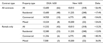
Table 2 reports the median nominal rent payments in 1650, in both the DGA dataset and in our new data, both as a whole and across the three subsamples. The last column reports the percentage difference between the 1650 median values. Figures in parentheses are the number of observations, which clearly illustrate why the DGA methodology cannot be extended beyond 1650: only a handful of commercial and mixed properties remain in the sample. This also suggests taking the comparison of rental values for such properties across the two datasets with a grain of salt.
Comparison of median nominal rents
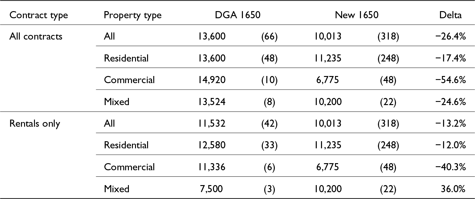
Table 2 Long description
The table compares median nominal rents for entire properties, in current maravedis, between DGA 1650 and New 1650, with sample sizes shown in parentheses. For all contracts and all property types combined, the median rent falls from 13,600 in DGA 1650 to 10,013 in New 1650, a decline of 26.4 percent. Under all contracts, residential rents drop from 13,600 to 11,235, mixed rents drop from 13,524 to 10,200, and commercial rents show the largest decrease from 14,920 to 6,775. Looking only at rentals, the overall median declines from 11,532 to 10,013, and residential rentals decline from 12,580 to 11,235. Commercial rentals also decline from 11,336 to 6,775, while mixed rentals rise from 7,500 to 10,200. Differences should be interpreted with caution because some categories have small sample sizes, especially mixed and commercial rentals.
Source: see the text.
Note: values are median rents for entire properties in current maravedis. Figures in parentheses are sample sizes.
The top half of the table uses all non-perpetual leases in the DGA dataset, capturing payments for all of short-term rentals, annual rentals, and lifetime leases. The overall difference in median housing payments across the two datasets is 26.4%, but a large portion of this gap is attributable to lifetime leases commanding higher payments to account for the inflation protection embedded in their long contract terms. The bottom half of the table restricts the properties in the DGA dataset to those under short-term and annual rental contracts, thus matching our new data. When doing so, the overall difference in housing payments is a drop of 13.2%. This is likely attributable to the DGA dataset being skewed toward richer properties.
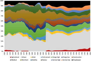
We next examine the distribution of renters’ occupations across both datasets. Figure 2 plots nine-year moving averages of the percentage of rental contracts awarded to tenants in each of 14 occupational categories. For the purpose of better illustrating the occupational distribution of tenants, this figure uses all types of contracts, including perpetuals.
Distribution of renters’ occupations (9-year moving averages).

Figure 2 Long description
The graph displays the distribution of renters′ occupations from 1500 to 1900. The horizontal axis represents years, while the vertical axis shows percentage from 0 to 100. Occupations include agricultural, artisan, artist, civil servant, clergy high, clergy low, construction, medical, merchant, nobility, notary, service high, service low and shopkeeper. The stacked layers represent the share of each occupation, with notable shifts around 1700. Agricultural and artisan occupations dominate early years, while service-related occupations increase later.
The transition between the two datasets reinforces the notion that the DGA data is somewhat more biased toward the top of the income distribution. After 1650, the share of artisans in the combined sample almost doubles, while the proportion of construction workers, agricultural workers, and service workers in low-skill occupations also increases significantly. Conversely, the weight of civil servants, clergy, notaries, and service workers in high-skill occupations decreases. The proportion of shopkeepers, artists, and merchants remains roughly the same. The final decline of Toledo’s economic fortunes in the eighteenth century is clearly seen through the lens of our new data. After 1700, the proportion of merchants and service workers in high-skill occupations steadily drops, replaced by an expansion in the share of agricultural and low-skill service workers.
Overall, the two datasets are reasonably well balanced at their point of contact. A 13% discrepancy in median rental values is no larger than some of the year-to-year variations in real rents introduced by swings in the prices of agricultural goods, for example. It is also a small magnitude in view of the very large range that the series exhibits over the long run. As long as the underlying data-generating processes are kept in mind, it is eminently possible to extract long-run trends and indices by combining the two datasets, a task to which we now turn.
4. The rental costs of entire properties
Real estate has, by definition, a large number of hedonic characteristics, all of which affect the rental cost of a given property. Creating rent indices, therefore, requires accounting for the impact of these hedonic factors. Since not all of them are equally available across our two datasets, we approach the task of constructing long-run series of rental costs in two steps. In this section, we focus on entire properties, the subsample for which Table 2 shows that the datasets can be reasonably well spliced. In the next section, we explore the cost of individual living spaces instead.
While all post-1650 payments recorded in the Carta Cuenta are for annual or short-term rentals, a majority of those before that date correspond to lifetime leases. When bidding for one of these long-term contracts, potential renters would have priced in the inflation protection afforded by the fixed nominal payments over a time span that could extend for decades. In an inflationary context, and assuming that leases were on average adjudicated at actuarially fair values, the annual payments over the first portion of the contract would have exceeded the value of housing services. Conversely, over the last portion of the contract, renters would have received housing services valued in excess of the nominal payment, now eroded by inflation.
Estimating the value of housing services from long-term lease data is a complex task. First, the relationship between the agreed-on payments and the actual value of housing services would have depended on inflationary expectations, which are unobservable. Second, a part of the payment was specified in live hens, which did not depreciate with the currency. Drelichman and González Agudo (Reference Drelichman and González Agudo2014) estimated a hedonic price index by relying on newly written contracts each year. This approach, however, is only possible with the pre-1650 data. It also restricts the average number of observations in any given year to less than five.
Here, we take the simpler approach of using the median rental payment for each type of property, neighborhood, or renter as our preferred measure of housing costs. For example, to establish the housing costs faced by working-class individuals, we can either take the median rent paid for individuals of a particular occupation or the median rental payment for properties in working-class neighborhoods. While this method ignores the difference between the contractual payment and the value of housing services for long-term leases, it has several other advantages. First, and trivially, it captures the rent payments actually made. If one wants to estimate the cost of living, it is hard to argue with using the cash and cash-equivalents actually paid each year, especially in an environment in which most people would have faced credit constraints. Second, the difference between the value of housing services and the actual payments made should average out across multiple contracts. While for new leases the annual payment would exceed the value of housing services, in long-running ones the converse would be true. By taking the median payment, conditional on observable characteristics, we should obtain a close approximation to the value of housing services. Finally, relying on the median payment allows us to use a consistent estimator across our two datasets, as hedonic estimation is not an option for the combined 1489–1810 data.
We begin our analysis by describing city-wide trends, and then gradually restrict it to specific groups, areas, and sub-periods.
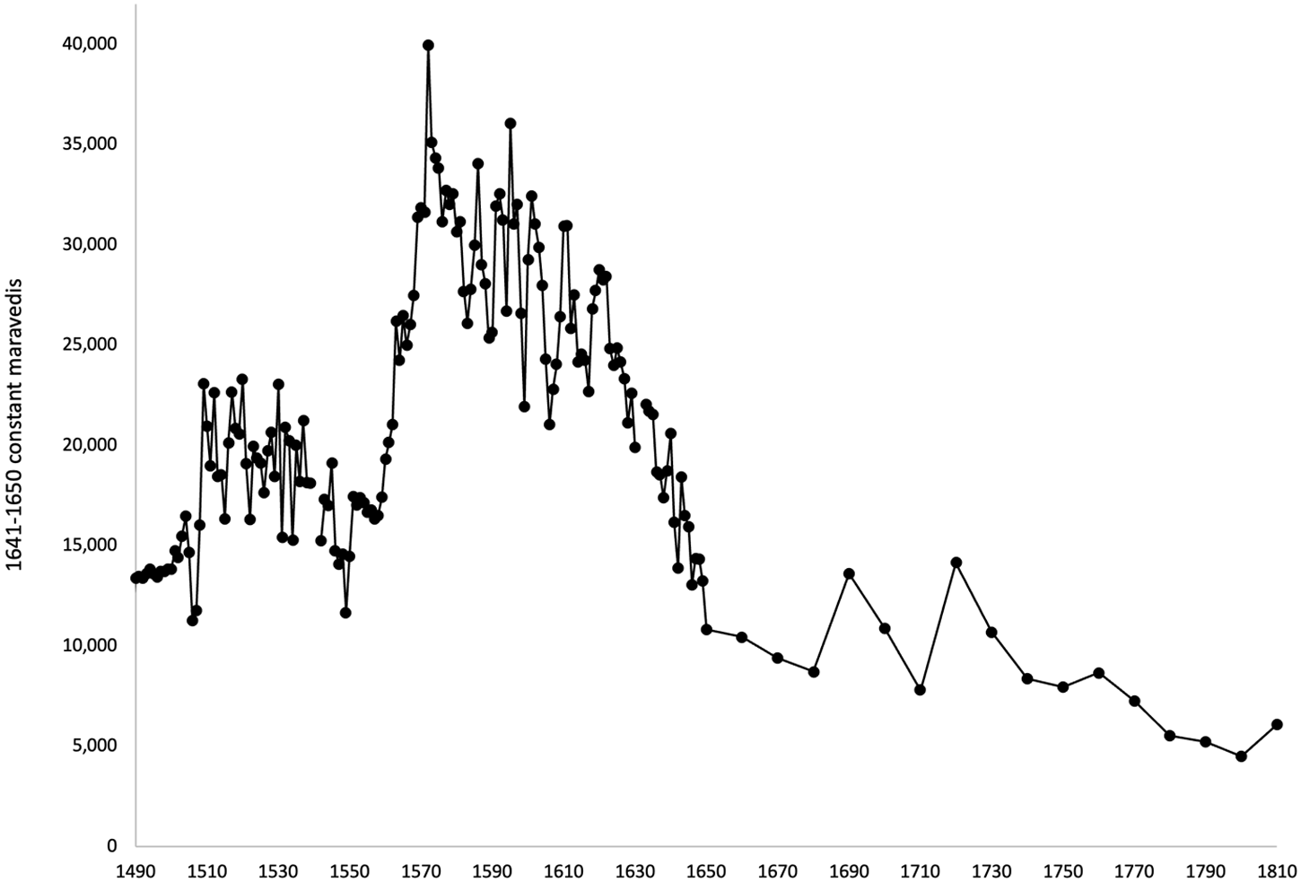
Figure 3 shows the median housing payment for entire residential properties across the entire city, for all sampled years, deflated using the Reher and Ballesteros (Reference Reher and Ballesteros1993) price index with a 1641–1650 base.Footnote 22 The series tells the story of Toledo’s fortunes. The second half of the sixteenth century, when American treasure fueled a construction boom and prominent figures of the nobility and the arts made Toledo their home, marked the peak of the rental market. The first half of the seventeenth century was just as dramatic, with plagues, famines, the centripetal force exerted by Madrid, and the increased local fiscal pressure all contributing to the fall in population and the attendant collapse of rental values. The eighteenth century saw a continued, if gradual, secular decline in real rents (the two peaks of 1690 and 1720 are the result of temporary drops in the deflator rather than increases in nominal rent payments). By 1810, at the height of the Peninsular War, the median Toledan residential property rented for 45% less than what it had in the late fifteenth century, and for a full 80% less than its real average value during the 1570–1595 years. We do note, however, that the physical characteristics and desirability of the median property also changed during this period, as we discuss more fully in the next section.
Median real housing payment.

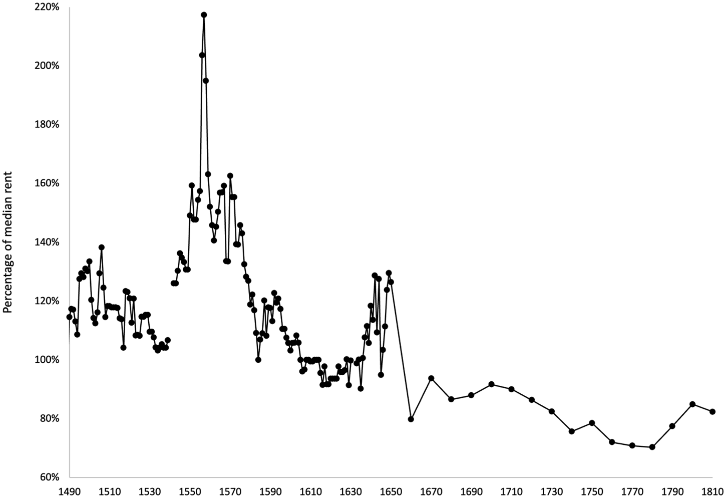
Figure 4 shows the interquartile range of housing payments for entire residential properties, plotted as a percentage of the median. As a measure of dispersion, the interquartile range can serve as an indicator of inequality through the lens of the rental market. The most salient feature is the stepwise increase between 1550 and 1570, with a large spike in the late 1550s. This corresponds to the sudden increase in median payments during the same period seen in Figure 3 and exactly matches the Dutch Disease process triggered by the inflow of American silver.Footnote 23 Dutch Disease is characterized by an increase in the price of non-tradable goods, of which housing is the quintessential example. The privileged classes, to whom the lion’s share of New World treasure accrued, bid up urban properties across several Castilian cities, transforming the urban landscape. Toledo was no exception; its most desirable residences were suddenly at a massive premium. New construction and urban renewal projects changed the face of the city during this time. By the mid 1575s, the pressure on Toledo’s limited land area started to push up the cost of more modest lodgings as well, thus reducing the dispersion in rental payments.
Interquartile range of real housing payments.

The second stylized fact that emerges from Figure 4 is the long-run decline in the interquartile range that starts in the late 1570s and continues through the end of the period, with a brief interruption in 1640–50 associated with the rapid collapse in rents in that decade. The secular decline is the result of the steady erosion of rental values at the top of the market and the associated compression of the rent spectrum as the high nobility and the merchant classes deserted the city.
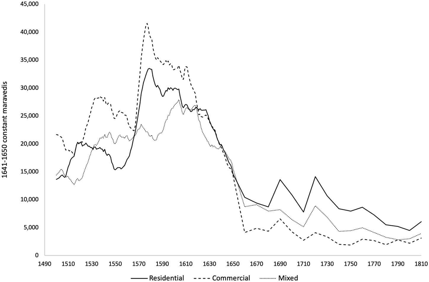
In addition to the residential properties discussed so far, Figure 5 adds commercial properties, defined as those destined exclusively for commercial use, and mixed properties, which had both residential and commercial elements.Footnote 24 The contrast between the sixteenth and the eighteenth centuries is stark. While commercial properties fetched the highest rents in the early period, they struggled to attract tenants in later times. Although some variation may be due to composition effects, the bulk of the Cathedral’s commercial real estate portfolio, focused on the neuralgic areas of Zocodover Square and the Alcaná crossing, stayed remarkably unchanged throughout the centuries; indeed, the Cathedral continues to own and rent out some of these very shops today.
Median real rents by property type.

One approach to characterizing the living standards of the different inhabitants of Toledo is to attempt a distinction between working-class and privileged neighborhoods. Martz (Reference Martz1983, 110) plotted a central “nexus of wealth” on a map of Toledo’s parishes, which Drelichman and González Agudo (Reference Drelichman and González Agudo2014) relied on to classify neighborhoods into rich and poor. A closer inspection reveals that Martz’s impression of Toledo’s wealthy areas does not correspond to the rental values or distribution of tenant occupations observed throughout the city. For example, while she places the entire parish of San Miguel outside the nexus of wealth, the areas of this parish adjacent to the Cathedral were home to three of the richest and most expensive properties in our sample. Conversely, Martz places the parish of Santa Leocadia, adjacent to the city walls, inside the wealth nucleus, but our data show that almost all properties in this area were small, rented for very modest amounts, and had few to no amenities.
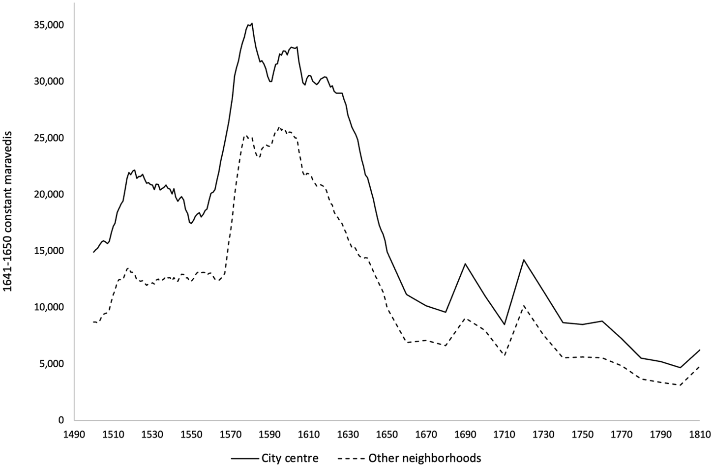
While it is tempting to define rich neighborhoods as those with higher rental values, this would be a form of identifying with the dependent variable. We prefer to adopt a rule based on the principles of the monocentric city model instead. We define the city center as a circle centered on the Cathedral, and with a radius of half the median distance to the city walls (301 meters). We then add Zocodover Square, the beating heart of the city’s commerce, to this central circle. Our rule allocates 30% of the urban area to the city center, with the remaining 70% belonging to the lower-lying neighborhoods.
Figure 6 shows median rental values for residential and mixed properties, in both central and lower-lying areas, throughout our entire period of analysis.Footnote 25 The ratio between them is remarkably stable, with rents in the city center generally averaging a 50% premium over those elsewhere. This result is strongly consistent with the monocentric city model, validating our rule to identify central and outlying areas. It is also consistent with working-class persons generally choosing to live farther away from the Cathedral and the market square.
Median real rent by area.

The Carta Cuenta lists the renter’s occupation for 21,492 renter/year pairs, amounting to 61.8% of all entries. Poorer tenants and those living far from the city center were less likely to have their occupation listed.Footnote 26 There are 594 different occupations, which we group into 15 ad-hoc categories and three broad socioeconomic groups, as reported in Table 3.Footnote 27
Occupational categories
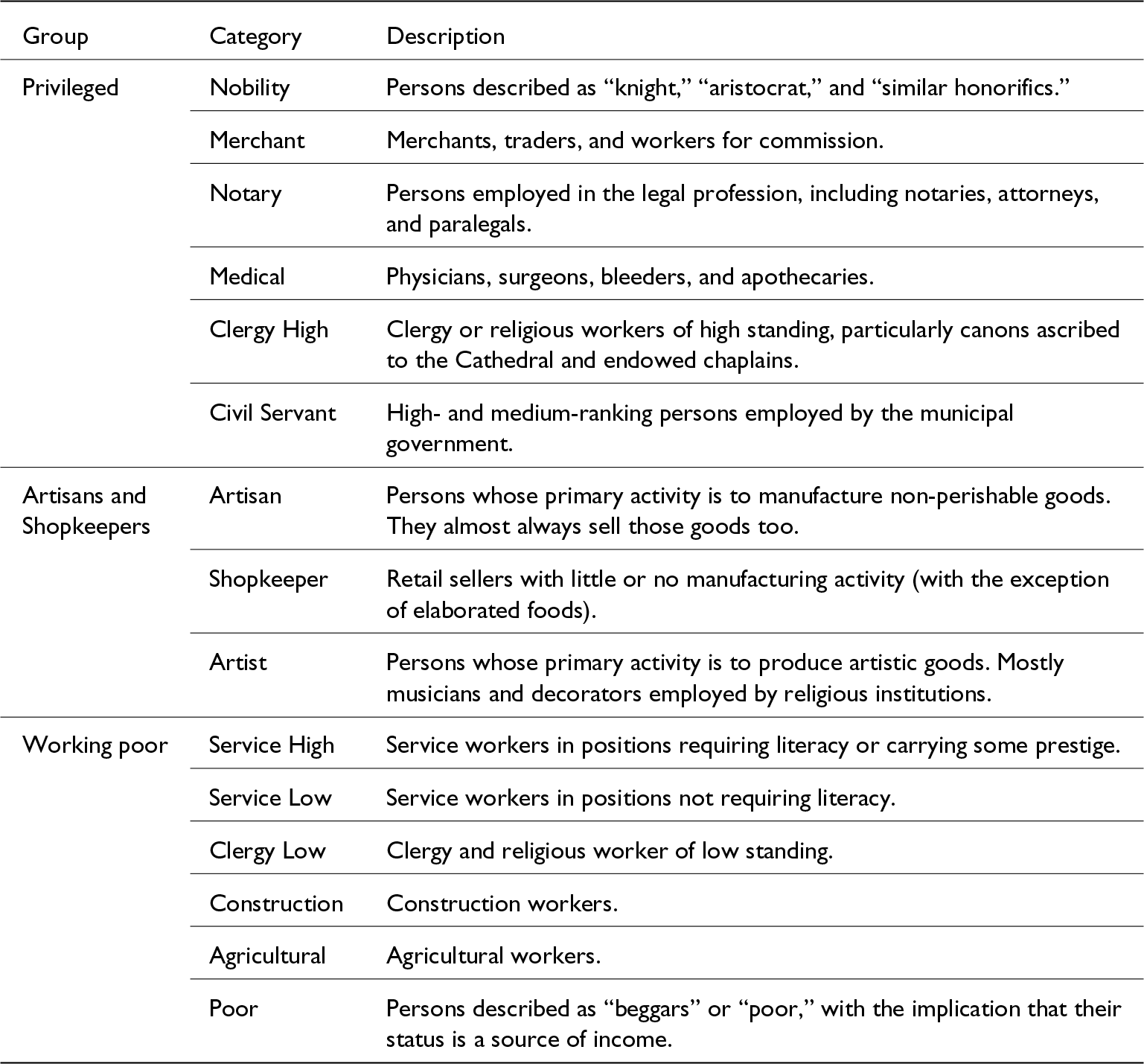
Table 3 Long description
The table defines an occupational classification system that assigns people to broad groups and specific categories, each with a short description of who is included. The Privileged group includes nobility identified by honorifics such as knight or aristocrat. Other standalone categories cover merchants, legal professionals such as notaries and attorneys, medical workers such as physicians and apothecaries, high-status clergy such as cathedral canons and endowed chaplains, and municipal civil servants of high or medium rank. Artisans and Shopkeepers are split into artisans who manufacture durable goods and usually sell them, shopkeepers who mainly retail with minimal manufacturing, and artists such as musicians or decorators often employed by religious institutions. The Working poor group includes higher-prestige or literate service roles, lower-status service roles, low-status clergy, construction workers, agricultural workers, and a Poor category for people labeled beggar or poor where that status implies income. Interpretations should note that some people with non-elite jobs may be classified as privileged if they held certain university degrees.
Source: see the text.
Note: any person holding a non-privileged occupation but holding the university degree of “Doctor” or “Licenciado” was added to the Privileged group.
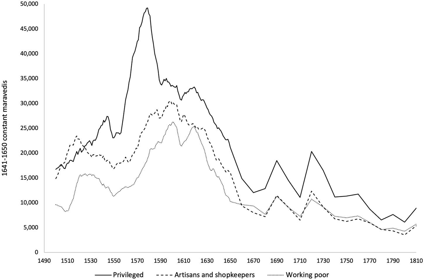
We can now analyze the evolution of rents paid by the different socioeconomic groups. As with the division by neighborhoods, we plot the median rents for entire residential and mixed-use properties in Figure 7.
Median real rent by socioeconomic group.

The rents paid by the three socioeconomic groups tell a compelling story about their relative standing through the centuries. In the early period, the skilled trades rented the most expensive properties, a trend that ended with the revolt of the Comunidades in 1521. Initially, Toledo, which was experiencing economic pressure from the stagnation of its manufacturing industries, joined the rebel side against the fiscal imposition and concentration of power by the new king, Charles I.Footnote 28 The privileged classes, however, soon switched their allegiance to the royalist party, which eventually prevailed. The ensuing repression and economic reparations altered the power dynamics of the city; Figure 7 shows that it also changed the groups that occupied the pricier lodgings. A second feature is the effect of American silver, which began arriving in earnest in the 1550s. Real rents increased for all socioeconomic groups, but disproportionately so for the privileged, who vied for a limited number of prestigious properties with a newly found source of liquid wealth. The end of the Dutch disease episode associated with the silver boom in the late 1570s was likely the major driver behind the collapse of privileged rent levels. It is also possible that the lower agricultural yields of the late sixteenth century, documented by López-Salazar Pérez and Martín Galán (Reference López-salazar Pérez and Martín Galán1981), might have contributed to a falling purchasing power of the higher classes. Llopis Agelán et al. (Reference Llopis Agelán, Antonio Sebastián Amarilla, Ubaldo Bernardos Sanz, Luis Velasco Sánchez and Abarca2018), however, have recently shown that the decline in yields in that period was not as marked, and might not have even happened in several Old Castilian locales.
Perhaps the most interesting trend is that of rents paid by artisans, shopkeepers, and artists, which can be roughly identified with the skilled middle class. Between 1490 and 1600, they paid an average of 47% more than the working poor. The premium dropped to 21% between 1600 and 1650, and disappeared entirely between 1660 and 1810. If rents are interpreted as a measure of purchasing power, Figure 7 can be seen as a poignant three-act story about the disappearance of Toledo’s middle class. From 1650 on, anyone who did not belong to the privileged strata lived in essentially the same type of quarters, regardless of occupation or skill.
A total of 5,571 primary renter entries in the Carta Cuenta are women, representing just over 15% of total renter-year pairs. 1,213, or 21.7% of them, are explicitly listed as widows; this is almost surely a lower bound, as several female long-term leaseholders whose marital status is not listed were in the second life of a three-life contract. Rents paid by women averaged 80% of those paid by men over the entire period of analysis, remarkably matching the long-run gender wage gap for Toledan nurses documented by Drelichman and González Agudo (Reference Drelichman and González Agudo2020).
Establishing the occupations of women is challenging. Only single women have an occupation listed. This results in a gap in the occupations of widows, many of whom would likely have continued to run the family shop or trade. Among single women, the most common listed occupational category is “Artisan,” with 116 entries. The next categories are “Clergy low” (nuns or “religious persons”), with 68 women listed; “Shopkeeper” (40 entries, with innkeeper being the most common job); and “Merchant” (13 entries). “Medical” (nurses), “Artists,” “Service high” (teachers), “Service low,” and “Poor” all have entries in the single digits.
5. Individual housing costs
Our analysis so far has centered on entire properties, as they offer the simplest way to splice the 1489–1650 and 1660–1810 datasets. The definition of what was an “entire property” certainly changed over time, and the nature of our data does not always allow us to observe these transformations. In the early period, large properties were rented out to intermediaries, who would sublease them in turn. Subleases were private transactions and are hence not recorded in the Carta Cuenta. In the late period, we observe rentals of fractions of houses, but we do not know the area of each of them. These two features make it challenging to construct time-consistent measures of the cost faced by individuals or families. In this section, we leverage the different characteristics of our datasets to propose two series of housing costs spanning the entire 1489–1810 period: one for the privileged classes and another for the peripheral areas where the majority of the working-class lived.
The 1489–1650 data contain entire properties only, but they also report the built area of each. The median size of houses intended for residential use in the Refitor’s portfolio during this period was 263 square meters, clearly well above the living space most people could afford. It is nonetheless straightforward to calculate the rent per square meter paid for any desired subset of properties or primary leaseholders; one simply divides the rent paid for the whole property by the built area.
In order to obtain the rental costs paid per individual in 1489–1650, we rely on two additional pieces of evidence. After estimating that the Cathedral owned 25% of Toledo’s real estate in 1571, Drelichman and González Agudo (Reference Drelichman and González Agudo2014, p. 42) calculated an average living space of about 15 square meters per inhabitant across the entire city. This value corresponds to the size of typical rooms. Clearly, wealthier families would have lived in larger spaces, while poorer ones would have crammed several people into a single room. We note that our data do not contain either the very poor or the very rich, as neither group would have rented their lodgings from the Cathedral. In the absence of further information on the distribution of living space across the city, we adopt a value of 15 square meters as the baseline individual living space for the working classes.
A second challenge is that, because of the Refitor’s practice of renting out whole properties up to 1625, the working poor are markedly underrepresented in the 1489–1650 data. We follow Drelichman and González Agudo (Reference Drelichman and González Agudo2014, p. 42) in proxying their rental expenditure with the rents commanded by properties in the least desirable neighborhoods. We therefore estimate individual rental costs for the working classes as the rent per square meter in non-central neighborhoods times 15 square meters.
The tenants we label “privileged” are actually a category that might be called the “working rich,” as opposed to the immensely wealthier landed aristocracy. They still lived in more spacious quarters and in wealthier areas of the city than the working poor. Since a large proportion of them belonged to the clergy, it is also more likely that they would have lived alone, rather than having to crowd a family into a single room. To estimate the living space for these wealthier persons in 1489–1650, we rely on the housing allowances paid by Tavera’s hospital, the largest healthcare institution in the city. Most of Tavera’s employees were entitled to accommodation as part of their contract. While many chose to live at the hospital itself, it was not unusual for white-collar employees, all of whom held jobs that fell in the “privileged” section of Table 3, to elect to receive a cash payment and procure their own housing instead. The median amount of these allowances was equivalent to the rental cost of 32 square meters in the more desirable central neighborhoods.Footnote 29 We therefore take 32 times the median rent per square meter paid by persons holding a “privileged” occupation as our measure of individual rental costs for the privileged classes between 1489 and 1650.
The 1650–1810 data, while not matched to an inventory with built area information, contain a large number of rentals described as aposentos, salas, and accesorias. In the singular, as they appear in the documentation, the terms aposento and sala refer to single rooms in a multi-room house. They would have been intended for the use of a small family and, in many cases, of a single individual, sharing entryways and common spaces with the tenants of other parts of the building.Footnote 30 Accesorias, which constitute the bulk of the fractional house rentals, were small apartments or coach houses with separate entrances. They were more variable in size, could have more than one room, and provided entirely private quarters.Footnote 31 As a starting point, we calculate the median cost of these fractional property rentals for non-central neighborhoods and for privileged individuals in each decadal year between 1650 and 1810.
The two datasets overlap in the year 1650. In the DGA dataset, the cost of 15 square meters in a peripheral neighborhood in 1650 is 920 maravedis; in our new data, it is 1887 maravedis, 2.05 times higher. It is therefore quite likely that the salas, aposentos, and accesorias in the 1650–1810 data would have been larger than the 15-square-meter definition we use for individual spaces in 1489–1650. In particular, since the data come from the same year, the ratio would imply that the accesorias, which constitute the majority of the fractional properties rented out, would have had a built area of around 30 square meters, and housed an average of two people.Footnote 32 In order to splice the two series, therefore, we divide the 1650–1810 fractional property rental series by the 2.05 ratio observed in the year of overlap. For the privileged rent series, the ratio is 1.66, likely reflecting a lower occupancy factor for dwellings rented by those of higher means. We therefore divide the 1650–1810 privileged fractional rent series by 1.66 in order to splice the two periods.
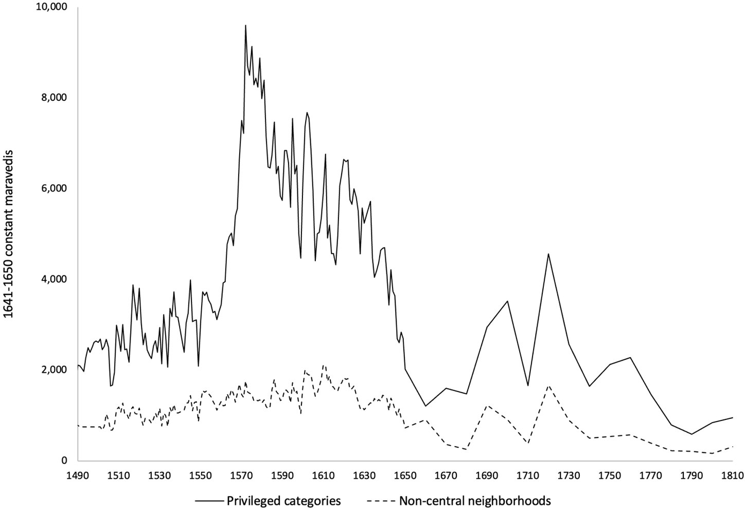
Figure 8 shows our estimates of real rental costs per person for privileged categories and for those residing in non-central neighborhoods, calculated as described above. The most salient feature of the chart is the decoupling of rents paid by the privileged from those in non-central neighborhoods between 1550 and 1590. This period coincides with the Peruvian silver boom, which accrued overwhelmingly to the rich. Luxury housing, being an eminently non-tradable good with a very inelastic supply, saw a threefold increase in its real value as demand skyrocketed. The market stabilized somewhat in the 1580s and 1590s, but did not return to pre-silver-boom levels until the 1630s, when the population exodus from Toledo began in earnest. By 1650, it was back to its 1490 mark.
Real rent per person.

The behavior of the market for properties favored by the privileged can be considered an extreme manifestation of Dutch disease, with bubble-like properties between 1550 and 1575. While the working poor also experienced rent increases on the order of 58% in real terms over the same period, they were not exposed to anything like the frenzy at the top of the market. The profile of the non-central neighborhoods’ rent series does not show any brusque discontinuity in the 1550s. In a common feature with the privileged series, it returned to its 1490s levels by 1650.Footnote 33
The second part of the period saw two peaks in real rents, in 1690–1700 and in 1720. Both are associated with deflationary processes; the first one is a result of the monetary stabilization of 1680, and the second one is caused by a 10-year decline in wheat prices. In both cases, as all other prices were falling, nominal rents increased by about 40%, compounding the impact of deflation on real rents. Both privileged and non-central neighborhood rents were affected in identical measure. A converse phenomenon occurred in the last quarter of the eighteenth century, when an inflationary process eroded the value of rents; this was further compounded by a fall in nominal rents.Footnote 34
A way to rationalize these dynamics is to consider housing as the residual budget item, capturing any family resources left over after satisfying the need for food. For the less-skilled part of the population, if city life became unaffordable because of rising prices, the remaining margin available was to move to the countryside; this would put downward nominal pressure on rent in times of inflation. Conversely, if food became cheap, more disposable income was made available to spend on housing. The limited building space available in Toledo would have contributed to amplify these forces through an inelastic supply curve.
Whether the unit of analysis are entire residences or individual living spaces, and regardless of the subsample under scrutiny, Figures 3 through 8 tell a remarkably consistent story. Toledan real rents closely tracked the fortunes of the city itself, soaring in its golden age, and plunging in times of crisis. By the time of the Napoleonic wars, and regardless of the group, area, or measure chosen, real rents in Toledo were about 50% lower than they had been in 1490.
6. Conclusion
Constructing a quality- and time-consistent series of expenditure on rent is an endeavor ridden with challenges and trade-offs. In our study, we select the city of Toledo, arguably more closely reflective of Spanish urban centers than the imperial capital of Madrid. We leverage the extensive records of its Cathedral chapter, which owned about 35% of residential real estate in the city. While the lack of an adequate inventory precludes us from replicating DGA’s hedonic analysis, we trade off their level of accuracy for much higher representativeness. We show that our new sample is reasonably balanced with the DGA data in their overlap year of 1650. We use different splicing approaches for our analyses of entire properties and of individual living spaces, and obtain the same broad results, reinforcing the idea that the two datasets are compatible. In particular, all our series follow the same pattern, showing a peak during the third quarter of the sixteenth century, rapid decline between 1630 and 1650, long-run stability until 1750, and a further 50% fall through the rest of the eighteenth century. By 1810, real rents in Toledo stood at half of their 1490 levels.
Our analysis of entire properties points to a commercial efflorescence in the first half of the sixteenth century, when the rents paid for commercial spaces exceeded those commanded by residential and mixed-use ones, and when artisans and shopkeepers paid higher amounts than even the privileged strata. This pattern came to an end in the wake of the Comunidades revolt, in which the Toledan bourgeoisie sided with the anti-royalist camp, leading to a sharp drop in its economic and political standing after its eventual defeat.Footnote 35 The next boom was different; fueled by American silver remittances, it was driven by the upper classes bidding up the rents of luxury properties. Rents paid by artisans and shopkeepers, as well as those of the working poor, increased as well, but not by the bubble-like magnitudes of those paid by the beneficiaries of the silver bonanza. The divergence subsided when the bankruptcy of 1575 and the increased fiscal pressure made necessary by the military defeats of the late 1580s called into question the lasting power of the new wealth stream.
The series of epidemiological and municipal policy crises that began in the late 1590s spurred a population exodus, ushering in a steeply declining phase for Toledo’s real estate and sounding the death knell for the city’s industrial base. By 1650, commercial rents, once the most expensive ones, had fallen below residential and mixed ones, while artisans and shopkeepers could no longer outbid the working poor when looking for living quarters. This new equilibrium reflected a city that had become a shell of its former self, retaining only its ecclesiastical character, as well as administrative functions for the surrounding countryside. Despite some attempts to revive the industrial sector via Royal chartered companies, this new equilibrium persisted more or less unaltered throughout the end of our period of analysis.
One key contribution of our work is to provide estimates of the living space and housing costs for individuals belonging to different social strata. Our “privileged” category reflects the most skilled and advantaged workers, who could afford relatively spacious quarters in the city’s better areas. We also use the rents from outlying neighborhoods as a proxy for those faced by the working poor. We find a notable decoupling between the two series, which is unlike anything observed in the rents paid for entire properties. The reason is that rents for entire houses are affected by composition effects, as the characteristics and spatial distribution of different property types changed through time. Our individual space series shows that the working poor were almost entirely bypassed by the silver-induced boom, in the sense that the rents they paid for their individual living space rose at about one-sixth of the rate of those faced by the privileged. They were also somewhat less affected by the monetary disturbances of the late seventeenth and early eighteenth centuries.
Historians sometimes take issue with the use of “decline” terminology to describe the demographic and economic crises that afflicted Spain throughout the long eighteenth century. At least from the perspective of housing costs in what was once Spain’s second-largest and possibly richest city, there are few other words that fit. After the bright light of the Siglo de Oro burned out, the dwindling population and vanquished industry depressed housing demand to the point that urban real estate fetched half the amount, in real terms, as it had in late medieval times. The rising costs of essential goods in the late eighteenth century delivered the final blow. Toledo, like many other Spanish cities, entered the nineteenth century devoid of the economies of agglomeration and the proto-industrial sector that would prove key to the industrial ascent of other parts of Europe.
Acknowledgements
We are grateful to Carlota Baltersee Fernández and to Ivana Pérez Luengas for excellent research assistance. We acknowledge funding from Proyecto PID2021-124378NB-I00 financed by MCIN/AEI/10.13039/501100011033/ and by FEDER Una manera de hacer Europa, from CIDER, and from two UBC WLIURA awards. All errors are ours.




 Open access

