


1. Introduction
Detrital sandstone composition is a key primary control for reservoir quality, and understanding regional and stratigraphic variability in composition can aid reservoir quality prediction. Typically, mineralogically mature, quartzose sandstones have a higher potential for good reservoir properties compared with feldspathic and/or lithic sandstones (e.g. Bloch, Reference Bloch and Wilson1994; Worden et al. Reference Worden, Mayall and Evans2000; Tobin & Schwarzer, Reference Tobin, Schwarzer, Scott, Smyth, Morton and Richardson2014). Sediment provenance is one of the main factors controlling the quartz–feldspar–lithic (QFL) composition. However, the original provenance signature may be overprinted or altered through the sediment-transport history and post-depositional alteration (Morton & Hallsworth, Reference Morton and Hallsworth1999). In recent years, inorganic geochemistry has been increasingly used to determine the mineralogy and provenance of sedimentary successions (e.g. Wright et al. Reference Wright, Ratcliffe, Bhattacharya, Zhu and Wray2010; Ikhane et al. Reference Ikhane, Akintola, Bankole, Ajibade and Edward2014), and can be particularly useful in regions where there is little or no core available for more traditional petrographic studies.
Bulk-rock geochemistry, primarily from cuttings samples, has been used in this study to investigate compositional changes through time in Paleocene–Eocene strata of Taranaki Basin, New Zealand. The deposits comprise a range of quartz arenites, subfeldsarenites and feldsarenites (classification according to Folk et al. Reference Folk, Andrews and Lewis1970), and are therefore characterized by highly variable feldspar abundance and type (e.g. Higgs & King, Reference Higgs and King2018). Previous petrographic studies suggest an increase in sandstone maturity from lower to middle Palaeogene strata (e.g. Higgs, Reference Higgs2002, Reference Higgs2010, Reference Higgs2013; Higgs & King, Reference Higgs and King2018), with highly mature quartz arenites being a particular feature of all Eocene strata in New Zealand (e.g. Bernet & Bassett, Reference Bernet and Bassett2016). The primary goal of this study was to investigate the use of downhole bulk-rock geochemical data to illustrate compositional changes from relatively feldspathic to relatively quartzose sandstones. Strata were analysed from a few, widely spaced wells (mostly > 40 km spacing) and constrained by a robust biostratigraphic framework in order to interpret regional trends in geochemistry and composition with respect to time and to changes in palaeoclimate. Results demonstrate how geochemical data can be used in stratigraphic and provenance studies and, in particular, how they might provide valuable insights into the geological understanding of areas that have limited datasets and few cored sections. Ultimately, this has implications both for predicting reservoir potential and as an analogue for ongoing climate change (Zeebe et al. Reference Zeebe, Ridgwell and Zachos2016; Forster et al. Reference Forster, Maycock, McKenna and Smith2020).
2. Geological setting
2.a. Study area and basin history
The Taranaki Basin is located predominantly offshore to the west of New Zealand’s North Island (Fig. 1), and forms one of a series of connected Cretaceous–Cenozoic basins that extend along western New Zealand (King et al. Reference King, Naish, Browne, Field and Edbrooke1999). Basin development was associated with the break-up of the eastern margin of Gondwana and formation of the Tasman Sea (Thrasher, Reference Thrasher1990; Bal, Reference Bal, van der Lingen, Swanson and Muir1994; King & Thrasher, Reference King and Thrasher1996; King et al. Reference King, Naish, Browne, Field and Edbrooke1999; Strogen et al. Reference Strogen, Seebeck, Nicol and King2017). Extensional faulting began during Late Cretaceous time with syn-rift depocentres locally persisting into the Paleocene Epoch and a subsequent passive margin represented by a prolonged (c. 30 Ma) period of tectonic quiescence (King & Thrasher, Reference King and Thrasher1996; Strogen, Reference Strogen2011). The tectonic regime started to change during late Eocene time in response to the development of a new plate boundary zone (Stagpoole & Nicol, Reference Stagpoole and Nicol2008; Strogen et al. Reference Strogen, Bland, Nicol and King2014); from early Miocene time, the eastern and southern parts of the Taranaki Basin were dominated by convergent margin-related tectonics (King & Thrasher, Reference King, Thrasher, Watkins, Zhiqiang and McMillen1992; Bull et al. Reference Bull, Nicol, Strogen, Kroeger and Seebeck2019).

Fig. 1. Taranaki Basin map showing study wells. Palaeogeography at 54 Ma shows the orientation of the middle Eocene palaeoshoreline and general position of facies belts for lower Eocene strata (after Strogen Reference Strogen2011). The present-day shoreline of the Taranaki Peninsula and latitude and longitude are also shown; see inset for location of the study area.
2.b. Palaeogene stratigraphy
Terrestrial to shallow-marine Palaeogene strata are subdivided by age and lithology into four formations that are thought to represent major second- to third-order depositional sequences (King & Thrasher, Reference King and Thrasher1996): (1) Paleocene–lowermost Eocene Farewell Formation; (2) lower–middle Eocene Kaimiro Formation; (3) middle–upper Eocene Mangahewa Formation; and (4) uppermost Eocene McKee Formation, with distal time-equivalent facies to these strata mostly represented by the marine Turi Formation (Fig. 2). These lower–middle Palaeogene strata form the focus of the current study. Upper Palaeogene strata comprise outer shelf to upper bathyal clastics and carbonates that were deposited following abrupt tectonically induced subsidence during latest early Oligocene time (King & Thrasher, Reference King and Thrasher1996), and are not included in the current study.
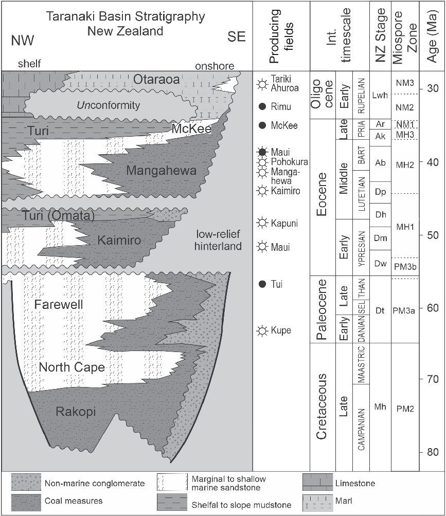
Fig. 2. Cretaceous and Palaeogene stratigraphic framework for the Taranaki Basin, New Zealand, plotted against the geological timescale and correlative miospore zones. The stratigraphic framework is modified from King & Thrasher (Reference King and Thrasher1996), international timescale from Gradstein et al. (Reference Gradstein, Ogg, Schmitz and Ogg2012) and miospore zones from Raine (Reference Raine1984, Reference Raine and Cooper2004). Dt – Teurian; Dw – Waipawan; Dm – Mangaorapan; Dh – Heretaungan; Dp – Porangan; Ab – Bortonian; Ak – Kaiatan; Ar – Runangan; Lwh – Whaingaroan.
Palaeogene strata and stage boundaries in New Zealand are based primarily on benthic and planktic foraminifera (Hornibrook et al. Reference Hornibrook, Brazier and Strong1989; Morgans et al. Reference Morgans, Beu, Cooper, Crouch, Hollis, Jones, Raine, Strong, Wilson, Wilson and Cooper2004), with stages correlated with the International Geologic Time Scale (Gradstein et al. Reference Gradstein, Ogg, Schmitz and Ogg2012) following Raine et al. (Reference Raine, Beu, Boyes, Campbell, Cooper, Crampton, Crundwell, Hollis and Morgans2015) (Fig. 2). However, the Paleocene–Eocene reservoir fairway is dominated by coastal to shallow-marine deposits, and calcareous microfossils (e.g. foraminifera) are rare. Miospore (spore and pollen) assemblages are typically well preserved in these facies and can provide robust age control using the zonal scheme of Raine (Reference Raine1984; revised in Raine, Reference Raine and Cooper2004) (Fig. 2).
2.c. Basement geology
Cambrian–Early Cretaceous basement rocks of New Zealand have been subdivided by Landis & Coombs (Reference Landis and Coombs1967) into Western and Eastern provinces. The former record early Palaeozoic terrane accretion and plutonism along the eastern Gondwana margin (Cooper, Reference Cooper1989; Tulloch et al. Reference Tulloch, Ramezani, Kimbrough, Faure and Allibone2009), while the latter represents Mesozoic accretion to the supercontinent (Coombs et al. Reference Coombs, Landis, Norris, Sinton, Borns and Craw1976; Howell, Reference Howell1980; Bradshaw, Reference Bradshaw1989).
The Western Province is considered to have been the main sediment source for Palaeogene strata in Taranaki Basin (Hill & Collen, Reference Hill and Collen1978; Smale & Morton, Reference Smale and Morton1987; Smale, Reference Smale1992, Reference Smale1996; Kamp, Reference Kamp2012; Higgs & King, Reference Higgs and King2018). It comprises the metasedimentary Takaka and Buller terranes (Cooper, Reference Cooper1989), which are intruded by a series of Devonian–middle Cretaceous batholiths/intrusives (Coombs et al. Reference Coombs, Landis, Norris, Sinton, Borns and Craw1976; Howell, Reference Howell1980; Tulloch, Reference Tulloch1988; Bradshaw, Reference Bradshaw1989; Mortimer, Reference Mortimer2004; Mortimer et al. Reference Mortimer, Rattenbury, King, Bland, Barrell, Bache, Begg, Campbell, Cox, Crampton, Edbrooke, Forsyth, Johnston, Jongens, Lee, Leonard, Raine, Skinner, Timm, Townsend, Tulloch, Turnbull and Turnbull2014; Tulloch et al. Reference Tulloch, Mortimer, Ireland, Waight, Maas, Palin, Sahoo, Seebeck, Sagar, Barrier and Turnbull2019). Overall, the Buller Terrane comprises mineralogically mature, quartzose sandstones, while the Takaka Terrane comprises a much wider range of lithologies, including volcanics, volcanoclastic sandstones and carbonates (Cooper, Reference Cooper1989). Plutonic rocks predominantly occur within two large batholiths, known as the Karamea and Median batholiths, but they also form smaller isolated plutons and batholiths throughout the Western Province (Tulloch, Reference Tulloch1983, Reference Tulloch1988). These rocks are collectively named the Tuhua Intrusives by Mortimer et al. (Reference Mortimer, Rattenbury, King, Bland, Barrell, Bache, Begg, Campbell, Cox, Crampton, Edbrooke, Forsyth, Johnston, Jongens, Lee, Leonard, Raine, Skinner, Timm, Townsend, Tulloch, Turnbull and Turnbull2014) and comprise several geochemical suites.
3. Methodology
Six study wells were selected for analysis along the Paleocene–Eocene reservoir fairway (Fig. 1), with a total of 458 geochemical analyses undertaken on Cretaceous–Palaeogene sediments and a few basement samples (Table 1). Most samples are from uncored sections, with samples taken from washed ditch cuttings at c. 20 m sampling intervals. A closer sampling interval of 3 m and 5 m was undertaken at Kupe South-4 for core and uncored intervals, respectively. Samples were collected from the New Zealand Petroleum and Minerals (NZP&M) National Core Store, and boreholes are close to vertical with depths or thicknesses quoted in metres (measured depth below Kelly bushing or bkb).
Table 1. Bulk-rock geochemistry samples from six wells, Taranaki Basin

Cutting samples were sieved to obtain the representative lithology, and obvious contamination was removed using a binocular microscope (e.g. mud additives, drill bit contamination, cavings). The samples were ground in agate and sample powders prepared by the alkali fusion procedure of Jarvis & Jarvis (Reference Jarvis, Jarvis, Hall and Vaughlin1992a, b). Major elements were analysed by inductively coupled plasma-optical emission spectrometry (ICP-OES) and trace elements by inductively coupled plasma-mass spectrometry (ICP-MS), with quantitative data acquired for 50 elements (see online Supplementary Material S1; http://journals.cambridge.org/geo). Precision errors are c. 2% for the major element data, c. 3% for the high-abundance trace-element data and c. 5% for most rare Earth elements (REE). All analyses were conducted at Chemostrat Ltd (UK).
Cuttings samples were assessed for potential caving and contamination by comparing chemically derived gamma-ray (Chem-GR) with wireline gamma-ray; the full suite of geochemical and Chem-GR data are provided in online Supplementary Material S1 and S2 (available at http://journals.cambridge.org/geo). Contamination issues were assessed by comparing the relative abundance of Ba and S, both of which are common drilling fluid additives. Cross-plots suggest that contamination is low in most samples, but has been identified in two wells (Turangi-3 and Kowhai-1A). The trace element Eu also shows a positive correlation with Ba at these two wells, which may reflect the interference of different Ba and Eu isotope peaks on the ICP-MS spectrum arising from drilling fluid contamination, and which was not corrected for at the time of analysis. Based on this information, the Ba, S and Eu data were excluded from interpretations at Turangi-3 and Kowhai-1A.
Heavy mineral analysis was undertaken on the 40–250 μm fractions of five samples from Kupe South-4 and a further four samples from offset well Kupe South-6. Heavy mineral grains were separated in a sodium heteropolytungstate solution (LST Fastfloat, 2.89 g cm–3) using the funnel separation technique (Mange & Maurer, Reference Mange and Maurer1992), and a representative portion of heavy mineral grains taken using a micro-splitter. The grains were mounted on a glass slide in Canada Balsam (refractive index (RI) of 1.55), and point-counted using a Nikon Eclipse polarizing microscope.
A well-constrained chronostratigraphic framework was developed for the six study wells using available palynology and foraminifera data (Raine, Reference Raine1984; Bartram et al. Reference Bartram, Sykes and Crouch1996; Higgs et al. Reference Higgs, Crouch and Morgans2006; Crouch, Reference Crouch2010; Raine & Mildenhall, Reference Raine and Mildenhall2011; Crampton et al. Reference Crampton, Morgans, Roncaglia, Reid, Schiøler, Raine and Fohrmann2012; Crouch & Raine, Reference Crouch and Raine2012; Raine & Schiøler, Reference Raine and Schiøler2012). In addition, geochemical results were integrated with published thin-section, x-ray diffraction (XRD) QEMSCAN®, trace-element geochemistry and U–Pb zircon geochronology data from relevant reservoir sandstones (Clews & Soo, Reference Clews and Soo1994; Higgs, Reference Higgs2010; Higgs et al. Reference Higgs, Strogen, Griffin, Ilg and Arnot2012b; Adams et al. Reference Adams, Campbell, Mortimer and Griffin2017) and volumetrically significant Devonian–middle Cretaceous granitoids (references provided in online Supplementary Material S3, available at http://journals.cambridge.org/geo). Alteration indices were used as one method to evaluate possible zones of enhanced chemical weathering through the Palaeogene interval and have been calculated from molecular proportions using chemical index of weathering (CIW; Harnois, Reference Harnois1988), plagioclase index of alteration (PIA; Fedo et al. Reference Fedo, Nesbitt and Young1995) and chemical proxy of alteration (CPA; Buggle et al. Reference Buggle, Glaser, Hambach, Gerasimenko and Marković2011).
4. Results and interpretation
4.a. Chronostratigraphic framework
Paleocene strata include the Farewell Formation (sandstones) and Turi Formation (mudstones) and are correlated with the PM3a miospore zone, and/or are assigned a Teurian (Dt = Danian–Thanetian) age from foraminiferal assemblages (Fig. 2). They are present in all study wells, with the thickest Paleocene intervals sampled for geochemical analysis in wells Kupe South-4 and Maui-4 (thicknesses of > 500 m and 400 m, respectively). Only the uppermost Paleocene strata have been analysed in other wells. For the purposes of this study, the Paleocene/Eocene (P/E) boundary is approximately correlated with the PM3a/PM3b miospore zonal boundary, although the P/E boundary is thought to occur slightly above this, within the lowermost part of the PM3b miospore zone (Ian Raine, pers. comm., 2018) (Fig. 2). Biostratigraphic data suggest that the P/E boundary has been penetrated in all six study wells, and sampling for geochemical analysis extends across the boundary in all cases (Fig. 3).

Fig. 3. Cross-section showing chronostratigraphic framework for the study wells; location of the transect is shown on the inset map, with legends on Figures 1 and 2 for facies belts and biostratigraphic data, respectively. Intervals sampled for geochemical analyses are indicated; mudstone/siltstone intervals are indicated by brown shading on the neutron-density (N-D) log crossover.
The earliest Eocene PM3b miospore zone represents a relatively short time interval (c. 2.5 Ma; Fig. 2) and is correlated with the lowermost Kaimiro Formation (sandstone) and time-equivalent Turi Formation (mudstones). The PM3b zone is relatively well constrained in four study wells where it reaches up to c. 170 m in thickness (Fig. 3). In Turangi-3, zone PM3b is not confidently identified, although it is assumed to be present based on similar log profiles within nearby well Kowhai A-1R. A discrete PM3b zone has not been identified in the more proximal well Maui-4; if present, it is likely to be a very thin or condensed interval (< 80 m thick PM3a/PM3b zone). A thin or absent zone has previously been recognized in lower Eocene coastal plain settings such as Pukeko-1 (cf. Fig. 1), where it is interpreted to be associated with significant fluvial incision (Higgs et al. Reference Higgs, Crouch and Raine2017). A very thin PM3b zone also occurs in Kupe South-4 (c. 30 m; Fig. 3) where it represents the only record of Eocene strata, unconformably overlain by Oligocene mudstones.
Most lower–middle Eocene strata in the Taranaki Basin are correlated with the MH1 miospore zone, which ranges in age from late Waipawan to early Porangan (lDw–eDp = Ypresian–Lutetian, c. 10 Ma duration; Fig. 2). The PM3b/MH1 zonal boundary has been cored at MB-P(8), where it is very sharp and possibly indicates a sequence boundary (Higgs et al. Reference Higgs, Crouch and Raine2017; Ian Raine, pers. comm., 2017). The MH1 zone is recognized in five of the study wells (absent from Kupe South-4) and corresponds to the main Kaimiro Formation reservoir. The MH1 zone is thickest in the most distal wells (> 500 m thickness at Turangi-3), thinning towards the more proximal Maui-4 well (< 100 m thickness; Fig. 3).
Regional marine transgression is recognized in the lower part of middle Eocene strata (Porangan Stage) at the MH1/MH2 zonal boundary, which resulted in deposition of the Omata Member and equivalent strata (Higgs et al. Reference Higgs, King, Raine, Sykes, Browne, Crouch and Baur2012a) (Figs 2, 3). The MH1/MH2 zonal boundary is well constrained in four study wells, inferred in Turangi-3 based on log correlation with Kowhai A-1R, and absent from Kupe South-4. The overlying MH2 miospore zone ranges in age from Porangan to early Kaiatan (Dp–eAk = Lutetian–Bartonian, c. 6 Ma duration; Fig. 2), and is correlated with the main Mangahewa Formation reservoir. A similar thinning pattern is observed in zone MH2, as is seen in the MH1 zone, with the thickest interval in the most distal wells (c. 600 m at Turangi-3 and Kowhai A-1R) and thinning in the most proximal well Maui-4 (c. 110 m). Sampling for geochemical analyses was not undertaken in the MH2 zone at Kowhai A-1R but was continuous to the top Eocene section in all other study wells (Fig. 3).
Miospore zones MH3 and NM1 are representative of uppermost Eocene strata, ranging in age from Kaiatan to Runangan (Ak–Ar = Bartonian–Priabonian, c. 3 Ma duration), and the zones are correlated with parts of the Mangahewa, McKee and Turi formations (Fig. 2). Chronostratigraphic control at this level is available for Kapuni-13 and Maui-4, with biostratigraphic data from offset wells Turangi-1 and Maui-2 used as a guide to uppermost Eocene correlation in wells Turangi-3 and MB-P(8), respectively. Despite the relatively short time interval for these zones, the MH3 interval is relatively thick in the distal wells (> 250 m at Turangi-1), and thinner (<100 m) in wells further west (MB-P(8) and Maui-4; Fig. 3).
The Paleocene–Eocene section forms the main focus of this paper. However, geochemical sampling was undertaken on older deposits in three wells. Upper Cretaceous strata, which are dated by miospore (zone PM2) and foraminiferal assemblages (Haumurian, Mh; Fig. 2), have been penetrated in two study wells. Geochemical sampling was undertaken in the uppermost part of Cretaceous strata in Maui-4 and through the entire penetrated Cretaceous interval in Kupe South-4 (Fig. 3). In addition, two wells penetrate igneous basement (Maui-4 and MB-P(8)) and bulk-rock geochemical data was acquired through both basement intervals to aid provenance discrimination.
4.b. Maui-4 and MB-P(8) basement correlation
Granite basement samples from MB-P(8) show a discrete and relatively mafic composition compared with samples from Maui-4 (SiO2, 52–55 v. 65–72 wt%; Cr, 92–120 v. 4–11 ppm; Ni, 40–43 v, 0.3–2.4 ppm; TiO2, 1.01–1.14 v. 0.18–0.49 wt%; e.g. Fig. 4a, b). Petrographic analysis has not been undertaken on these cuttings samples. However, age data from previous work have established that the granites represent part of the Carboniferous and Cretaceous Median Batholith (U–Pb zircon ages of c. 328 Ma at Maui-4 and c. 115 Ma at MB-P(8); Tulloch & Mortimer, Reference Tulloch and Mortimer2017), with probable age correlation to the Foulwind Suite at Maui-4 (cf. Tulloch et al. Reference Tulloch, Ramezani, Kimbrough, Faure and Allibone2009) and either Separation Point or Rahu suite at MB-P(8) (cf. Tulloch & Kimbrough, Reference Tulloch, Kimbrough, Johnson, Patterson, Fletcher, Girty, Kimbrough and Martín-Barajas2003). However, there is a significant range in the geochemical composition of all the igneous suites (e.g. Tulloch, Reference Tulloch1983; Muir et al. Reference Muir, Weaver, Bradshaw, Eby and Evans1995, Reference Muir, Ireland, Weaver, Bradshaw, Evans, Eby and Shelley1998; Tulloch & Kimbrough, Reference Tulloch, Kimbrough, Johnson, Patterson, Fletcher, Girty, Kimbrough and Martín-Barajas2003; Allibone et al. Reference Allibone, Jongens, Scott, Tulloch, Turnbull, Cooper, Powell, Ladley, King and Rattenbury2009; Tulloch et al. Reference Tulloch, Ramezani, Kimbrough, Faure and Allibone2009), which makes it difficult to confirm these correlations on the basis of their geochemical signature (e.g. Fig. 4). Additionally, basement samples may have undergone different levels of alteration, which can change their geochemistry and thereby make correlations more difficult. Significantly, basement samples from MB-P(8) display very high alteration indices (CIW = 76–90, compared with 48 of average andesite where SiO2 = 58 wt%), which could be indicative of moderate to significant chemical weathering and would be consistent with the well completion description as a basement wash (STOS, 1994). In contrast, Maui-4 basement samples have moderate alteration indices (CIW = 55–60 and SiO2 = 65–72 wt%), which are intermediate between average andesite and rhyolite (CIW = 62 and SiO2 of 73 wt%) and would be consistent with fresh (unaltered) samples.

Fig. 4. Geochemical plots for basement samples from Maui-4 and MB-P(8) showing: (a) La/Sc v. Zr/Sc; (b) SiO2 v. TiO2; (c) Rb v. Sr/Y; and (d) Y v. Nb. (c, d) Plotted with published geochemical data from selected igneous suites; references provided in online Supplementary Material S3. These trace elements and ratios are some of the best discriminators (e.g. Tulloch & Kimbrough, Reference Tulloch, Kimbrough, Johnson, Patterson, Fletcher, Girty, Kimbrough and Martín-Barajas2003) but still illustrate the wide variability in suite composition. (e, f) Chondrite-normalized rare Earth element (REE) patterns comparing (e) basement samples from Maui-4 and MB-P(8), and (f) selected published data from McCulloch et al. (Reference McCulloch, Bradshaw and Taylor1987), Muir et al. (Reference Muir, Weaver, Bradshaw, Eby, Evans and Ireland1996), Waight et al. (Reference Waight, Weaver, Muir, Mass and Eby1998), Price et al. (Reference Price, Spandler, Arculus and Reay2011) and Sagar et al. (Reference Sagar, Palin, Tulloch and Heath2016).
Given the above, together with the small number of samples analysed, the basement correlation at Maui-4 and MB-P(8) has been primarily based on the U–Pb zircon ages of Tulloch & Mortimer (Reference Tulloch and Mortimer2017). Samples from Maui-4 overlap the ranges for most major and trace elements of published data from the Foulwind Suite (Fig. 4c–f), and are therefore consistent with a Foulwind correlation. Samples from MB-P(8) display a geochemical signature that falls outside the typical range of published data from the Separation Point Suite (Fig. 4c–f), but given the high alteration indices it is suggested that these differences could largely be due to the effects of chemical weathering. While the data are equivocal, a Separation Point Suite is favoured over the Rahu Suite for MB-P(8) basement based on (a) the mafic composition, which has a much lower SiO2 content than all known samples from the Rahu Suite, and (b) the location of MB-P(8), which is further east than known occurrences of the Rahu Suite.
4.c. Mineral affinities of elements, Palaeogene sandstones
Bulk-rock geochemical data from lower–middle Palaeogene sandstones have been compared with available petrographic data to establish element–mineral affinities. Interpretations are primarily based on data from well MB-P(8), which has a long (c. 190 m) Eocene cored interval, and well Kupe South-4, which has a shorter (c. 66 m), dominantly Paleocene, cored interval. The element–mineral affinities determined from petrographic data are confirmed by bivariate relationships observed for sandstone lithologies from the full geochemical dataset (plots presented in online Supplementary Material S4, available at http://journals.cambridge.org/geo). A summary of the key elements and ratios that have been used in this study to characterize the lithology and sandstone composition are presented in Table 2. Other trends observed between high-field-strength elements are mostly attributed to heavy mineral composition, and are discussed further in Section 4.g.
Table 2. Key bulk-rock elemental data, ratios and alteration indices

CIW – chemical index of weathering (Harnois, Reference Harnois1988); CPA – chemical proxy of alteration (Buggle et al. Reference Buggle, Glaser, Hambach, Gerasimenko and Marković2011); PIA – plagioclase index of alteration (Fedo et al. Reference Fedo, Nesbitt and Young1995)
4.c.1. Eocene sandstones, MB-P(8)
Lower Eocene sandstone core from MB-P(8) is described by Clews & Soo (Reference Clews and Soo1994) as having a quartzo-feldspathic composition and comprising fine-grained through to coarse-grained, granular subarkose and arkose. Other grains have been described as trace to minor rock fragments (mostly plutonic) and trace to abundant accessories (mostly biotite mica with only rare heavy minerals).
Reasonably close matches are observed between the downhole profiles of certain elements (this study) and minerals (Clews & Soo, Reference Clews and Soo1994), despite differences in sample depths and sample type between the XRD and geochemistry samples (core and cuttings, respectively). These relationships support probable element–mineral affinities for SiO2 and quartz, K2O and K-feldspar, and Na2O and plagioclase (Fig. 5); CaO values are very low, which indicates that plagioclase is dominantly albite (Na rich). Clay-fraction XRD data from MB-P(8) (Clews & Soo, Reference Clews and Soo1994) show that illite/mica (K2O rich) and smectite (Na2O/CaO rich) are rare or absent in most of the sandstone samples. Only the argillaceous sandstones are reported to contain minor illite; in these lithologies, some of the measured K2O and associated very high Cs/Rb ratios will be associated with this clay (Fig. 5). Kaolinite, described as authigenic by Clews & Soo (Reference Clews and Soo1994), is the dominant clay mineral within the MB-P(8) sandstones. However, only a moderate relationship is observed between total clay (measured from XRD) and Al2O3, which is interpreted to be due to the association of Al2O3 with both feldspar and clay minerals (mostly kaolinite).

Fig. 5. Comparison of x-ray powder diffraction (XRD) data from core samples (Clews & Soo, Reference Clews and Soo1994) with bulk-rock elemental data from cuttings (this study) plotted against gamma-ray (GR), neutron-density (N-D) and biostratigraphy (Bio) data for well Maui B-P(8). Whole-rock XRD data are plotted as bar charts (dark colour) joined by a bar edge line (pale colour). Elemental data are represented by coloured disks. Mudstone/siltstone intervals are indicated by brown shading on the N-D log crossover. Alteration indices after Harnois (Reference Harnois1988), Fedo et al. (Reference Fedo, Nesbitt and Young1995) and Buggle et al. (Reference Buggle, Glaser, Hambach, Gerasimenko and Marković2011).
Whole-rock XRD data demonstrate the patchy distribution of carbonate cements in cored sandstone samples. Calcite is a relatively rare carbonate cement in the petrographic samples (Clews & Soo, Reference Clews and Soo1994), which is consistent with low CaO. Siderite and dolomite are more common, occurring predominantly in the upper cored section (Fig. 5) where they are represented by coincident peaks of MgO, Fe2O3 and MnO. However, coincident peaks of MgO, Fe2O3 and MnO are also recognized in the lower cored section where siderite and ferroan dolomite have typically not been identified. Based on XRD and thin-section observations, other Fe-rich minerals (pyrite, chlorite, biotite) are all more abundant in the lower cored section (Clews & Soo, Reference Clews and Soo1994), and are therefore the likely main mineral affinities at this stratigraphic level.
Heavy minerals have not been identified from XRD and are reported in trace amounts from thin-section; for this reason, heavy minerals cannot be used to establish element–mineral affinities. However, the abundance of heavy rare Earth elements (HREE) may give an indication of heavy mineral abundance (see online Supplementary Material S4, available at http://journals.cambridge.org/geo), with HREE strongly related to lithology (Fig. 5). Notably, ratios of some high-field-strength elements (HFSEs; e.g. Hf/Sc, Zr/Y, Ta/HREE) are elevated in the sandstones, which implies relative enrichment of zircon and Ti-bearing heavy minerals over more mafic (and labile) heavy minerals. This is consistent with the few identified heavy minerals reported from thin-section (opaques, limonite and zircon, and rare garnet and tourmaline; Clews & Soo, Reference Clews and Soo1994).
4.c.2. Paleocene–Eocene sandstones, Kupe South-4
Palaeogene sandstones from core and sidewall core (SWC) at Kupe South-4 have been described by Martin et al. (Reference Martin, Baker, Hamilton and Thrasher1994) as very fine-grained through to very coarse-grained sandstones, mostly of lithic arkose or feldspathic litharenite composition, where igneous fragments (predominantly quartz–feldspar) are the most abundant lithic grain types. Martin et al. (Reference Martin, Baker, Hamilton and Thrasher1994) note a downhole reduction in quartz abundance, which is mostly compensated for by an increase in plagioclase feldspar, but is also associated with an increase in biotite and heavy minerals (epidote, sphene).
A comparison of geochemistry and thin-section data show reasonably close matches between the profiles of SiO2 and quartz, and Na2O and plagioclase, and a fair match between K2O and K-feldspar (Fig. 6), providing further evidence for these as probable element–mineral affinities. A very clear break in major-element geochemistry is noted close to the top of Paleocene strata (uppermost zone PM3a) at c. 3.1 km depth, where deeper samples are characterized by low SiO2 and high Na2O and K2O values. Mineralogically, these changes reflect the downhole increase in plagioclase relative to quartz reported by Martin et al. (Reference Martin, Baker, Hamilton and Thrasher1994). Petrographic data indicate that K-feldspar does not appreciably increase with depth, and the higher K2O observed through most of the Paleocene–Cretaceous section will reflect additional K-rich minerals (e.g. illite/mica). In the shallower well section, total clay content from point count data shows a good match with both Al2O3 content and alteration indices. XRD confirms that the clay fraction is predominantly kaolinite, which has been described by Martin et al. (Reference Martin, Baker, Hamilton and Thrasher1994) as authigenic, formed from the decomposition of biotite, feldspar and rock fragments. Al2O3 content in the upper well section is therefore mostly interpreted to be associated with kaolinite and, to a lesser degree, feldspar. In the lower well section (below c. 3.1 km), Al2O3 content is relatively constant with no apparent match to point-counted total clay; this is interpreted to be due to an overall greater affinity of Al2O3 to plagioclase feldspar.

Fig. 6. Comparison of point-count data from core samples (Martin et al. Reference Martin, Baker, Hamilton and Thrasher1994) with bulk-rock elemental data from cuttings (this study) plotted against gamma-ray (GR), neutron-density (N-D) and biostratigraphy (Bio) data for well Kupe South-4. Petrographic data are plotted as bar charts (dark colour) joined by a bar edge line (pale colour). Mudstone/siltstone intervals are indicated by brown shading on the N-D log crossover. Alteration indices after Harnois (Reference Harnois1988), Fedo et al. (Reference Fedo, Nesbitt and Young1995) and Buggle et al. (Reference Buggle, Glaser, Hambach, Gerasimenko and Marković2011).
Mineralogical affinities of the other major elements are more difficult to establish, which probably suggests that they are associated with a variety of clay, carbonate and heavy minerals. The profile shape of CaO bears little resemblance to point-counted carbonate, suggesting that calcite is not a significant component of these deposits. Conversely, in the upper well section (above c. 3.1 km), coincident peaks of Fe2O3, MnO and, to a lesser extent, MgO display a spikey response with some degree of match to the counted carbonate. Although geochemical and petrographic samples are from different depths, these results are considered sufficiently similar to indicate that Fe2O3, MnO and MgO are predominantly associated with carbonates in this upper part of the stratigraphy. Qualitative XRD analysis confirms that siderite is the main carbonate phase, and is relatively common in the upper well section (Martin et al. Reference Martin, Baker, Hamilton and Thrasher1994).
A significant shift is observed in the baseline concentration of CaO, MgO, Fe2O3 and MnO to overall higher and more consistent values below c. 3.12 km. The relatively consistent geochemical response is due, in part, to a change in sample type from core (uppermost section) to cuttings (lower section). However, carbonate has not been recorded from most petrographic samples from the lower well section, suggesting that CaO, MgO, Fe2O3 and MnO have other mineral affinities through this interval. QEMSCAN data from Higgs et al. (Reference Higgs, Strogen, Griffin, Ilg and Arnot2012b) show that plagioclase in Paleocene sandstones at Kupe South-4 includes a significant component of Na–Ca plagioclase (see Section 4.d.2); this is considered to be the main host for CaO below c. 3.12 km. However, qualitative clay fraction XRD data also demonstrate a change in clay mineralogy from the upper kaolinite zone to a thick underlying interval where mixed layer chlorite–smectite is the dominant clay (Martin et al. Reference Martin, Baker, Hamilton and Thrasher1994). These clays will account for some of the CaO and Na2O in the lower well section, while a good match between Fe2O3, MgO and relative abundance of chlorite–smectite indicates that these clays are also the main hosts for Fe and Mg (Fig. 6). A greater abundance of biotite and heavy minerals identified from thin-section analysis (Martin et al. Reference Martin, Baker, Hamilton and Thrasher1994) can also account for some of the MgO, Fe2O3, CaO and MnO, as well as TiO2 and REE. Overall, HREE values are fairly high through most of the Cretaceous–Eocene section, consistent with relatively common heavy minerals, while similar profiles for HREE, SiO2 and total point-counted clay again demonstrate a relationship between HREE and lithology. Notably, ratios of some HFSEs imply a stratigraphic change in the heavy mineral suite, consistent with the uphole reduction in epidote and sphene (cf. Martin et al. Reference Martin, Baker, Hamilton and Thrasher1994) and indicative of relative zircon and Cr-bearing heavy mineral enrichment (e.g. high Hf/Sc and Zr/Y showing a good match with Ta/HREE, Cr/Ce, Cr/Y and Cr/Th).
4.d. Major-element geochemistry
The established mineral affinities of elements have been used to interpret and compare sandstone composition through lower–middle Palaeogene strata. Key elemental data are presented for well MB-P(8) and summarized for all study wells to illustrate systematic stratigraphic and/or geographic changes. Previous workers have used major oxide ratios of SiO2, Al2O3 and, to lesser extents, MgO and Fe2O3 to distinguish sandstone lithologies from mudstone/siltstone (e.g. Sprague et al. Reference Sprague, Melvin, Conradi, Pearce, Dix, Hill and Canham2009; Ikhane et al. Reference Ikhane, Akintola, Bankole, Ajibade and Edward2014). However, it is clear that high Al2O3 concentrations in Palaeogene samples do not necessarily reflect mudstone/siltstone lithologies due to the presence of locally feldspathic and kaolinitic sandstones. In this study, an SiO2/Al2O3 ratio of > 4 together with low Cs/Rb and high K2O/Rb ratios (typically ≤ 0.05 and ≥ 0.035, respectively) have been used for sandstone identification.
4.d.1. MB-P(8)
Middle–upper Eocene sandstones (Mangahewa Formation, zone MH2) are typically characterized by high SiO2 (72–87 wt%, mean 81 wt%), low K2O (1.1–2.7 wt%, mean 1.6 wt%) and low Na2O values (1.1–2.7 wt%, mean 0.7 wt%; Fig. 7). These results suggest that the sandstones are quartzose with low volumes of total feldspar. Relatively high K2O/Rb ratio values (> 0.037) indicate that much of the available K2O is associated with K-feldspar rather than illite/mica, while relatively high K2O/Na2O ratio values (c. 2–4.5) indicate that within these feldspar-poor sandstones, K-feldspar is more abundant than Na-feldspar (albite). This interval is also characterized by very low background MnO and CaO, with a rare coincident peak interpreted to represent the local presence of minor carbonate cements (C in Fig. 7).

Fig. 7. Bulk-rock elemental data for key elements and ratios plotted against gamma-ray (GR), neutron-density (N-D) and biostratigraphy (Bio) data for well Maui B-P(8). Mudstone/siltstone intervals are indicated by high GR and brown shading on the N-D log crossover, while mudstone/siltstone cuttings are indicated by low SiO2 and K2O/Rb together with high Cs/Rb (shown by brown shading on Cs/Rb and K2O/Rb profiles). Note that locally the geochemical data are not representative of the drilled interval (shown by red box and demonstrated by an elevated chem-GR in online Supplementary Material S2).
Lower–middle Eocene sandstones from MB-P(8) (Kaimiro Formation, zone MH1) also contain some samples with high SiO2 (up to 89 wt%) with a similar major-element signature to the younger Mangahewa Formation. However, several samples from the Kaimiro Formation are characterized by lower SiO2 (68–89 wt%, mean 77 wt%) associated with variable Na2O (0.4–2.1 wt%, mean 1.3 wt%) and very high K2O (2.1–3.4 wt%, mean 2.7 wt%), suggesting that locally the sandstones are relatively feldspathic. Very high K2O/Rb ratio values (up to c. 0.055) are again evidence that K2O is mostly associated with K-feldspar (Fig. 7).
Sandstone samples of earliest Eocene (zone PM3b) and Paleocene (zone PM3a) age display a variable low-to-moderate SiO2 content (64–77 wt%, mean 69 wt%). High SiO2 contents (i.e. SiO2 > 80 wt%) are not recorded through this interval, which is likely due to the relatively high K2O (2.2–3.2 wt%, mean 2.7 wt%) and consistently high Na2O (1.7–2.8 wt%, mean 2.4 wt%) below the MH1/PM3b zonal boundary (Fig. 7). High K2O and Na2O values are interpreted to reflect highly feldspathic sandstone compositions, while very low K2O/Na2O ratio values (1–1.7) indicate that Na-feldspar (albite) is likely to be more abundant than K-feldspar. This change in major-element concentration highlights a significant difference in sandstone composition between the older (Paleocene and earliest Eocene) and the younger (Eocene) sandstones.
The K2O/Rb ratio appears slightly suppressed in the Paleocene sandstones (zone PM3a) compared with Eocene sandstones (zones PM3b to MH2), and this could be an indication of relatively high clay contents within the stratigraphically older deposits (Fig. 7). Sharp coincident peaks of MnO and CaO are again interpreted within the lowermost Eocene and Paleocene interval (zones PM3b and PM3a) to represent carbonate-cemented zones (C in Fig. 7). However, background MnO and CaO concentrations in Paleocene–lowermost Eocene lithologies are higher than those of overlying Eocene lithologies (zones MH1 and MH2), which could potentially reflect a change in clay, feldspar and/or cement mineralogy.
4.d.2. Regional correlation
Multi-well plots of key elemental data and ratios show that the significant change in Na2O content, observed close to the PM3b/MH1 zonal boundary in well MB-P(8), also occurs in other study wells. Above the PM3b/MH1 boundary, most sandstone intervals are characterized by high SiO2, high K2O/Rb ratios and relatively low Na2O values, suggesting that they are dominated by quartz and K-feldspar with relatively minor plagioclase. Below the PM3b/MH1 boundary, most sandstone intervals are characterized by lower SiO2 and higher Na2O, reflecting a plagioclase-rich affinity (Fig. 8).

Fig. 8. Cross-section through study wells showing vertical changes in SiO2, K2O/Rb, K2O and Na2O plotted against gamma-ray (GR), biostratigraphy (Bio) and QEMSCAN data. Mudstone/siltstone cuttings are indicated by brown shading on K2O/Rb data.
Background MnO and CaO levels are low throughout much of the Eocene section (zones MH1 and MH2, Fig. 9), although local spikes of MnO (without coincident CaO spikes) do occur in some of the mudstone/siltstone intervals, and likely represent concentrations of Mn in clays and/or heavy minerals. Coincident peaks of MnO and CaO, interpreted to represent carbonate-cemented zones, are particularly prolific through the Eocene section at Kapuni-13 (Fig. 9). Overall, background MnO and CaO are higher in the older Paleocene and Cretaceous strata (zones PM3a and PM2), associated with the higher concentrations of Na2O (Fig. 9) and with relatively high concentrations of TiO2, Fe2O3, MgO, P2O5 and many trace elements (Table 3). It is suggested here that the higher CaO content reflects a component of Na–Ca plagioclase, which has been shown from QEMSCAN data (Higgs, Reference Higgs2010; Higgs et al. Reference Higgs, Strogen, Griffin, Ilg and Arnot2012b) to be very rare in Eocene strata of the Taranaki Basin but relatively common in Paleocene and Cretaceous strata. It is notable that the presence of Na–Ca plagioclase is associated with high total feldspar and where plagioclase is more abundant than K-feldspar (Fig. 10). Elevated levels of other elements in the older strata are interpreted to reflect an increase in the abundance of mafic and/or heavy minerals (e.g. TiO2, MnO, Nb, Sc, Y, REEs) and a change in phyllosilicate mineralogy to higher biotite and possibly chlorite/smectite (e.g. Fe2O3, MgO, REEs).

Fig. 9. Cross-section through study wells showing vertical changes in SiO2, Na2O, MnO and CaO plotted against gamma-ray (GR), biostratigraphy (Bio) and QEMSCAN data.
Table 3. Average abundance of selected oxides and trace elements by stratigraphy. All – all analysed cuttings; sand – sandstone cuttings based on lithology indicator cut-offs defined in Table 2. Eocene strata (representing MH1, MH2, MH3 zones) contain the lowest abundances of most elements, with the exception of Hf and Zr (zircon affinity), Cr and Ta.


Fig. 10. Relative proportions of feldspars from QEMSCAN data (Higgs et al. Reference Higgs, Strogen, Griffin, Ilg and Arnot2012b) with bulk-rock elemental data (this study) plotted against gamma-ray (GR) and biostratigraphy (Bio) data for wells Kapuni-13 and Kupe South-4. Fdsp refers to total feldspar abundance (vol%) to nearest percent; relative proportion of feldspar types are illustrated by pie charts.
These geochemical results are evidence for a regional change in sandstone composition across the PM3b/MH1 zonal boundary. However, the trend is complicated by the fact that the lowermost Eocene deposits (zone PM3b) are relatively argillaceous in many wells and represent a period of overall transgression across western Taranaki Basin. Another complication is that few Eocene strata are preserved at Kupe South-4, where only the lowermost part of the PM3b zone is present and the geochemical change in composition occurs at a slightly lower stratigraphic level (Figs 6, 9). The change in composition is abrupt in most wells, with the exception of Turangi-3, which is the most distal study well and where a more gradual decline in Na2O is observed from the PM3b zone upwards through the MH1 zone (Fig. 8).
A second, later regional change in major-element composition is suggested by a relatively gradual increase in Na2O concentration, which has been observed towards the top of the study interval (Fig. 8). This increase in Na2O in uppermost Eocene deposits (zone MH3) may reflect a return to relatively plagioclase-rich deposits and/or an upwards increase in smectite content. The increase in Na2O is accompanied by an increase in CaO, which could either be related to the reintroduction of Ca-plagioclase or could reflect a change towards carbonate-rich facies close to the Eocene–Oligocene boundary.
4.e. Alteration indices
Geochemical indices of alteration are high through all mudstone/siltstone-dominated intervals, which is primarily a response to high Al2O3 concentrations in these lithologies (Fig. 11). While alteration indices are variable through the sandstone lithologies, they are also locally very high (CIW, 75–90). Several authors have used these indices to describe the degree of mineral alteration (e.g. Parker, Reference Parker1970; Vogel, Reference Vogel1975; Nesbitt & Young, Reference Nesbitt and Young1982; Harnois, Reference Harnois1988; Fedo et al. Reference Fedo, Nesbitt and Young1995; Buggle et al. Reference Buggle, Glaser, Hambach, Gerasimenko and Marković2011), and it is possible that some very high indices in the Palaeogene sandstones could be indicative of significant chemical weathering. There are, however, inherent problems that need to be considered when interpreting alteration indices for stratigraphic studies (e.g. Garzanti & Resentini, Reference Garzanti and Resentini2016), and results should be evaluated in conjunction with other data.

Fig. 11. Cross-section through study wells showing vertical changes in Cs/Rb, Al2O3/Alkali (Al/Ak = Al2O3/(CaO+MgO+K2O+Na2O)), alteration indices (Alt In) and Na2O plotted against gamma-ray (GR) and biostratigraphy data (Bio). Molecular proportions have been used in the calculation of alteration indices, where CaO* is the estimated silicate Ca. CIW – chemical index of weathering ((Al2O3/(Al2O3+CaO*+Na2O))×100; Harnois, Reference Harnois1988); PIA – plagioclase index of alteration (((Al2O3–K2O)/(Al2O3+CaO*+Na2O-K2O))×100; Fedo et al. Reference Fedo, Nesbitt and Young1995); and CPA – chemical proxy of alteration ((Al2O3/(Al2O3+Na2O))×100; Buggle et al. Reference Buggle, Glaser, Hambach, Gerasimenko and Marković2011). Mudstone/siltstone cuttings are indicated by brown shading on Cs/Rb data.
Multi-well plots show that the highest sandstone alteration indices occur above the PM3b/MH1 boundary in wells Maui-4, MB-P(8) and Kapuni-13, decreasing slightly uphole in upper Eocene strata (MH2 and MH3 zones; Fig. 11). Very high indices are also apparent within slightly older deposits (uppermost zone PM3a–PM3b) below the top Eocene unconformity at Kupe South-4, associated with depleted Na2O and CaO (Figs 6, 11). The lowest sandstone alteration indices occur in upper Cretaceous, Paleocene and lowermost Eocene strata at Maui-4, MB-P(8) and Kapuni-13 (zones PM2, PM3a and PM3b respectively). However, alteration indices are also relatively low through the Eocene section in the more distal wells Turangi-3 and Kowhai A-1R, with a further decline into the uppermost Eocene (Fig. 11). Differences between the Paleocene and Eocene cannot be determined in these two distal wells due to the dominance of fine-grained (clay-rich) lithologies through the penetrated Paleocene strata.
These results further support a significant change in sandstone composition resulting in an overall reduction in alkali elements relative to Al2O3 above the PM3b/MH1 boundary. This could have been caused by loss of plagioclase through weathering/diagenesis, a change in sediment provenance and protolith composition, and/or due to sedimentary/hydrodynamic effects.
4.f. Heavy mineral analysis, Kupe South-4 and -6
The main components of heavy mineral assemblages at Kupe South-4 and -6 are tourmaline, titanite (sphene), zircon and apatite (Table 4), all of which are common accessory minerals in granitoid rocks. Less abundant are epidote and garnet, both of which are commonly associated with greenschist-facies metamorphic rocks, but are also indicative of some intrusive rocks. Although variations are observed between the samples, overall the heavy mineral suites of Kupe South-4 and -6 are comparable to suite 4 of Smale (Reference Smale1992), which has previously been interpreted to represent derivation from metamorphic and granitic rocks of the NW Nelson area.
Table 4. Heavy mineral abundance (vol%) from wells Kupe South-4 and Kupe South-6. Other – sum of abundance of amphibole, anatase, andalusite, clinozoisite, clinopyroxene, diaspore, sillimanite and topaz; co – core; cu – cuttings

Results show high recovery of heavy minerals for three samples from Kupe South-4 and three samples from Kupe South-6; all are from the Paleocene (zone PM3a). A significant reduction is observed in the two samples taken near the P/E boundary with very few heavy minerals recovered from the single lower Eocene sample (zone PM3b). This uphole reduction in heavy mineral abundance is accompanied in Kupe South-4 by a significant increase in the proportion of ultrastable tourmaline, which is particularly abundant in the lower Eocene sample. Both wells are characterized by an uphole increase in the ZTR (zircon–tourmaline–rutile) index (Table 4), and all heavy minerals, with the exception of zircon, show significant corrosion features. Collectively, these data might imply that the uppermost (younger) samples have a heavy mineral signature indicative of greater degrees of chemical/mechanical weathering compared with the lower samples.
Samples with the lowest amounts of both tourmaline and zircon (Kupe South-4, 3116.9 and 3321 m, Kupe South-6, 3300 m) are dominated by titanite (sphene), which can largely account for the high TiO2 recorded in Paleocene strata and Eocene mudstones. These samples also contain the highest proportion of epidote (8.2–17.9 vol% of heavy mineral fraction), which is less stable than zircon and tourmaline. It is notable that small amounts of olivine and orthopyroxene have been identified from the sample taken from the top of the Paleocene strata in Kupe South-4 (3082.7 m); orthopyroxene has only been identified in very small quantities in two other samples. Both olivine and orthopyroxene are particularly unstable; their initial abundances (i.e. at the time of sediment deposition) might therefore have been higher, representing remnants of a largely altered heavy mineral suite derived from ultramafic–mafic igneous rocks. Alternatively, the very low abundance of these minerals might be indicative of an additional (minor) sedimentary source. Absence from the uppermost (late Eocene) sample could be due to complete dissolution within a highly altered zone, or a change in the sediment source.
4.g. Basement–sandstone correlation
The quartzo-feldspathic composition (Sections 4.c, 4.d) and heavy mineral suite (Section 4.f) of lower–middle Palaeogene sandstones in Taranaki Basin is consistent with a dominant source from the Tuhua Intrusives. Additionally, chondrite-normalized REE plots for the Palaeogene samples are comparable to REE profiles of the igneous basement samples from MB-P(8) and Maui-4, showing enrichment of LREE over HREE (see online Supplementary Material S5, available at http://journals.cambridge.org/geo). Very slight to moderate negative Eu anomalies are evident for most Palaeogene samples, which could suggest a dominant felsic source rock, but alternatively could be related to loss of plagioclase during weathering. Clear evidence for Na2O depletion (and in some cases CaO depletion), reflecting a reduction in plagioclase content, has been noted in Eocene strata relative to the igneous basement samples and to Cretaceous–lowermost Eocene strata (Fig. 12).

Fig. 12. Selected cross-plots showing the distinct major-element composition of basement samples at Maui-4 and Maui B-P(8) and a comparison between basement and Paleocene sandstone composition in wells (a) Maui-4, (b) Maui B-P(8) and (c) Kapuni-13, where sandstone lithology has been based on a cut-off for SiO2/Al2O3 and K2O/Rb. Plots illustrate the higher Na2O content of Cretaceous to lowermost Eocene sandstones (PM3a, PM3b) and uppermost Eocene sandstones (MH3) compared with the main Eocene reservoir sandstones (MH1 and MH2).
High-field-strength elements associated with heavy minerals are unlikely to have been influenced by weathering or diagenesis, and are therefore commonly used in provenance studies (e.g. McLennan et al. Reference McLennan, Hemming, McDaniel, Hanson, Johnsson and Basu1993). Positive trends have been observed for several elements, although many relationships are fairly broad, suggesting that most elements are associated with a variety of heavy minerals. At least two positive trends, related to well location but unrelated to stratigraphy, are developed between some immobile elements. For example, samples of Cretaceous–Eocene age from Kupe South-4 and Kapuni-13 display lower Nb/TiO2 and Ta/Nb, and higher TiO2/Ta, Th/Ta and U/Ta compared with samples from other study wells (see online Supplementary Material S4). These plots confirm that there was a spatial change in sediment provenance across the study area, with the HFSEs interpreted to reflect contributions of heavy minerals derived from different igneous suites. Overall, trace-element ratios of Palaeogene sandstones from MB-P(8), Turangi-3 and Kowhai-A1R are most similar to published data from the Separation Point Suite, while Cretaceous and Palaeogene sandstones from Kapuni-13 and Kupe South-4 have more mafic compositions that are most similar to data from the Darran Suite (e.g. Fig. 13a). There is no clear evidence for a dominant source from the Karamea Suite in any of the study wells (e.g. high Nb, Rb; Figs 4, 13a).

Fig. 13. Geochemical plots for basement and sandstone samples from all study wells showing (a) Y v. Nb; and (b) La/Sc v. Hf/Sc. Sandstone lithology has been based on a cut-off for SiO2/Al2O3 and K2O/Rb. (a) > 90% data fields based on published geochemical data from selected igneous suites (references provided in online Supplementary Material S3).
Detrital zircon age data are available from a previous study for a single Cretaceous sandstone within the sampling interval at Maui-4 (2841–2844 m; Adams et al. Reference Adams, Campbell, Mortimer and Griffin2017), confirming provenance from the Tuhua Intrusives. However, zircon ages also show that there has been input from several different igneous suites (c. 44% zircon from the Separation Point/Rahu Suite, 13% from the Darran Suite, 29% from mid-Palaeozoic suites, 13% from Buller/Takaka metasedimentary rocks). Notably, while detrital zircon data suggest that Separation Point Suite was the dominant source for this Maui-4 sample, the Y–Nb plot indicates that the Darran Suite was dominant (Fig. 13a). This discrepancy could perhaps be explained by lower zircon fertility of the Darran Suite, although that would need to be proven from further research. It is suggested here that several igneous suites are likely to have contributed sediment to the Palaeogene interval at all study locations (cf. Higgs & King, Reference Higgs and King2018), which, together with the wide-ranging composition of suites, makes source identification from geochemistry problematic.
In addition to spatial trends in immobile trace elements, some trends have been observed that appear related to stratigraphy. Overall, the Cretaceous–Paleocene lithologies display a much tighter geochemical signature compared with a more variable geochemistry of Eocene lithologies, while the few samples from uppermost Eocene strata have compositions that are most similar to the Cretaceous–Paleocene samples (Fig. 13). Other observed trends are not consistent across all locations, and probably reflect local changes in source area with time (Fig. 13a). Notably, however, enrichment of Hf and Zr occurs relative to Sc within many Eocene sandstones from all wells (Fig. 13b). Given the strong affinity of Hf and Zr with zircon (see online Supplementary Material S4), this could either imply removal of relatively reactive minerals prior to deposition (i.e. enhanced chemical and/or physical weathering), or an uphole change to a more felsic, zircon-rich sedimentary source. The former is favoured here because La/Sc and Th/Sc remain approximately the same, while Zr/Sc and Hf/Sc increase sharply; Th/Sc and La/Sc would be expected to track Zr/Sc and Hf/Sc if the relative zircon enrichment was primarily due to a change in provenance. It is also notable that in most wells the Cr/Y ratio values increases in Eocene sandstones, being locally higher than Cr/Y values from published data for the Tuhua Intrusives, and significantly greater than Cr/Y values of both Eastern and Western Province metasedimentary rocks (e.g. Roser et al. Reference Roser, Coombs, Korsch and Campbell2002). As Cr and Y are both relatively immobile elements, if they co-exist in a mineral then relative enrichment of Cr over Y due to chemical weathering/alteration is unlikely. However, high Cr/Y values could be explained if the Cr originated from resistant heavy minerals (e.g. tourmaline, rutile, titanite and ilmenite/magnetite) and Y was at least partially present (and lost) in relatively reactive heavy minerals (e.g. garnet). High Cr/Y ratios could also reflect concentrations of clinopyroxene (i.e. increased mafic material input); however, clinopyroxene is very unstable and high concentrations would be diametrically opposed to zircon enrichment. On this basis, it is suggested that relatively high Cr within some of the Eocene sandstones is most likely due to concentrations of resistant heavy minerals, either resulting from an evolving sediment provenance (relatively enriched in these minerals) or from enhanced chemical/physical weathering.
Overall, the trace-element data from Kupe South-4 is very constant, suggesting that at this location there has not been an appreciable change in provenance through Cretaceous–earliest Eocene time. However, there is a very clear change in some HFSE occurring at the same stratigraphic level as a significant change in the major-element geochemistry (Fig. 6). Elevated Hf/Sc and Zr/Y show a good match with high Ta/HREE, Cr/Ce, Cr/Y and Cr/Th, which is interpreted to represent relative zircon and Cr-bearing heavy mineral enrichment, and is consistent with a change in the heavy mineral suite from sphene-dominated (Paleocene) to zircon-tourmaline (lowermost Eocene). Given the constant ratios of other immobile trace elements, together with high alteration indices and extensive kaolinitization (Martin et al. Reference Martin, Baker, Hamilton and Thrasher1994) of uppermost Eocene strata, these data imply that the significant differences in major-element composition between the older and younger strata in this well is indeed primarily due to alteration.
5. Discussion
Clear trends in major-element geochemistry have been observed through the Cretaceous–Eocene succession in Taranaki Basin that relate to stratigraphic changes in sandstone composition. Paleocene (and Upper Cretaceous) sandstones display a mineralogy that is most comparable to the plutonic basement rocks that underlie much of the basin and crop out in the northern South Island (Tulloch, Reference Tulloch1983, Reference Tulloch1988; Mortimer et al. Reference Mortimer, Tulloch and Ireland1997; Rattenbury et al. Reference Rattenbury, Cooper and Johnston1998). These rocks are composed primarily of plagioclase (up to c. 50 vol%, mostly albite with locally significant An60) with subordinate quartz, K-feldspar, biotite and minor clay and heavy minerals. By comparison, Eocene sandstones display a mineralogy that is enriched in quartz and K-feldspar compared with both Paleocene sandstones and known basement compositions. The most significant change in geochemical signature occurs across the PM3b/MH1 zonal boundary and is abrupt in relatively proximal wells Maui-4, MB-P(8) and Kapuni-13, but appears more gradual in the most distal well Turangi-3. We suggest that this could be due to fluvial incision, erosion and/or non-deposition in some of the relatively proximal wells in response to the Kaimiro sequence boundary (cf. Higgs et al. Reference Higgs, Crouch and Raine2017) (Fig. 14). A more subtle change back to relatively sodic plagioclase-rich sandstones also occurs in uppermost Eocene strata (miospore zone MH3). Possible reasons for the observed stratigraphic changes in Palaeogene mineralogy are discussed below.

Fig. 14. Summary figure showing the interpretations for the observed stratigraphic changes in major-element geochemistry and quartz–feldspar composition. The stratigraphic framework is modified from King & Thrasher (Reference King and Thrasher1996), international timescale from Gradstein et al. (Reference Gradstein, Ogg, Schmitz and Ogg2012) and miospore zones from Raine (Reference Raine1984, Reference Raine and Cooper2004). The Taranaki basement map is modified from Tulloch & Mortimer (Reference Tulloch and Mortimer2017) and palaeogeography maps modified from Strogen (Reference Strogen2011). The Palaeogene palaeoclimate estimate is based on TEX86H records for New Zealand (red dashed line being the 3-point moving average), which is a proxy for sea surface temperature, from Hollis et al. (Reference Hollis, Dunkley Jones, Anagnostou, Bijl, Cramwinckel and Edgar2019).
5.a. Change in sediment provenance
The earliest Eocene period (PM3b zone, Fig. 2) marks the onset of the post-rift phase in parts of southern Taranaki (King & Thrasher, Reference King and Thrasher1996; Strogen et al. Reference Strogen, Seebeck, Nicol and King2017), which resulted in flooding of Paleocene depocentres and deposition of marine mudstone across much of the southern basin. All the central basement ridges would have become submerged, and subsequent Eocene strata were deposited on an intra-continental passive margin that was virtually undisrupted by contemporaneous faulting (King & Thrasher, Reference King and Thrasher1996; Stagpoole & Nicol, Reference Stagpoole and Nicol2008; Strogen, Reference Strogen2011). It therefore seems plausible that a change in sedimentary provenance might have occurred in response to this significant change in the southern basin morphology during latest Paleocene–earliest Eocene time.
Despite changes in tectonic regime, the distribution of preserved Paleocene and Eocene strata in Taranaki Basin is similar, and implies a southern eroding hinterland dominated by igneous intrusives and subordinate Western Province metasediments (Fig. 14). A slightly larger area of the southern hinterland may have been exposed during Eocene time, while drowned basement ridges that defined Cretaceous syn-rift sub-basins may have been capable of shedding some sediment during deposition over the Paleocene Epoch. Although the Tuhua Intrusives in the southern hinterland collectively formed the dominant sediment source throughout Palaeogene–Eocene time, there will have been subtle changes in contribution from the different plutonic suites as the drainage patterns changed through time. Sediment contribution from metasedimentary rocks (Eastern and Western provinces) is unproven but not considered to have been dominant through Cretaceous–Eocene time, as supported by the limited detrital zircon data (cf. Higgs & King, Reference Higgs and King2018), dominance of igneous lithics (e.g. Martin et al. Reference Martin, Baker, Hamilton and Thrasher1994; Chemostrat Ltd, 2017; Higgs et al. Reference Higgs, Funnell and Reyes2013, Reference Higgs, Crouch and Raine2017) and geochemical signatures.
It is difficult to confirm or demonstrate changes in igneous source based on the bulk-rock geochemistry. This is partly because of the very wide range of chemical compositions recorded in the literature for individual suites, but also because of sediment contribution from multiple suites. Using current knowledge on the distribution of intrusives from Tulloch & Mortimer (Reference Tulloch and Mortimer2017), based purely on proximity, the dominant igneous source rocks for lower–middle Palaeogene sandstones may have been the Darran and Longwood suites in the east (Kupe South-4, Kapuni-13) and Separation Point or Foulwind suites in the west (MB-P(8), Maui-4), with possible local contribution from other less extensive suites (e.g. Rahu, Tobin and Tarpaulin suites; Fig. 14). The immobile trace-element geochemistry supports a mixed sedimentary source, and is also consistent with different source contributions to eastern and western parts of the basin that are related to basement proximity (Fig. 13a).
It is possible that the regional stratigraphic change from plagioclase-rich to quartz–K-feldspar-dominated sandstones reflects an overall change in provenance from dominantly intermediate–mafic sources to relatively felsic sources in the earliest Eocene. Known felsic sources include the I-type Separation Point, I-/S-type Rahu, and S-type Karamea and Ridge suites (e.g. Muir et al. Reference Muir, Weaver, Bradshaw, Eby and Evans1995; Tulloch et al. Reference Tulloch, Ramezani, Kimbrough, Faure and Allibone2009; Tulloch & Palin, Reference Tulloch and Palin2013), with extensive Separation Point and Karamea granitoids mapped to the south and west of all study wells (Tulloch, Reference Tulloch1988; Tulloch et al. Reference Tulloch, Ramezani, Kimbrough, Faure and Allibone2009; Tulloch & Mortimer, Reference Tulloch and Mortimer2017). These felsic granitoids are likely to have formed a more significant eroding hinterland during Eocene rather than Paleocene time (Fig. 14 and figs 11–13 of Higgs & King, Reference Higgs and King2018) and could explain the greater variability in geochemical signature of Eocene compared with Paleocene lithologies. Provenance for Paleocene sandstones in southern Taranaki (i.e. Manaia/Pakawau sub-basins) is therefore likely to have been from relatively local basement highs due to the residual rift basin topography (e.g. Smithies et al. Reference Smithies, Bassett, Browne and Nichols2019), while the provenance for Eocene sandstones may reflect more mixing and, potentially, sources from further afield. Relatively quartzose-, K-feldspar-rich Eocene sediments would have been transported via longshore drift across a broad shelf, with further quartz and resistant heavy-mineral enrichments from transportational winnowing, re-working and progressive weathering of less-resistant minerals. The geochemical data are, however, not entirely consistent with a simple change from dominantly mafic–intermediate sediment sources (Cretaceous–earliest Eocene) to felsic-sourced sediment (early–late Eocene). Instead, the trends observed in HFSE ratios are interpreted to reflect local changes in depositional facies, provenance and drainage patterns which are overprinted by the more significant regional change in major-element geochemistry, and detrital composition across the PM3b/MH1 boundary.
Major-element, immobile trace-element and petrographic data are all consistent with a return to plagioclase-rich deposits during latest Eocene time. This period represents the start of an episode of tectonic uplift and erosion in the eastern part of the basin, as a far-field manifestation of the proto Australian–Pacific plate boundary propagating to the east (Strogen et al. Reference Strogen, Bland, Nicol and King2014, Reference Strogen, Higgs, Griffin and Morgans2019). A dominantly mafic provenance is likely from either the exposed Tuhua Intrusives in the south and SE, or from eroding Cretaceous–Paleocene strata located to the east of the present-day Taranaki Basin margin. Locally, Eastern Province zircons have been recorded from the NE part of Taranaki Basin in uppermost Eocene strata (e.g. Kamp, Reference Kamp2012), which, together with the introduction of metasedimentary lithic clasts in this part of the basin, would be consistent with some sediment derivation from the east at this time (Higgs & King, Reference Higgs and King2018).
5.b. Chemical weathering and/or alteration
Substantial evidence has been presented to suggest there has been preferential weathering and/or alteration of sediment during Eocene time; significant Na and Ca depletion is observed above the PM3b/MH1 boundary; elevated Hf/Sc, Zr/Y, Cr/Ce, Cr/Y and Cr/Th occur in Eocene deposits (indicating relative enrichment of zircon- and Cr-bearing heavy minerals); Eocene sandstones are impoverished in heavy minerals and dominated by a resistant suite compared with Paleocene sandstones; Eocene strata are characterized by higher alteration indices than older Cretaceous–Paleocene sandstones. These data are supported by other studies that have demonstrated considerable feldspar alteration within some Eocene sandstones associated with secondary kaolinite precipitation (e.g. Clews & Soo, Reference Clews and Soo1994; Higgs et al. Reference Higgs, Funnell and Reyes2013, Reference Higgs, Crouch and Raine2017), extensive kaolinite in the uppermost Paleocene–lowermost Eocene interval in the Kupe South Field reflecting alteration of unstable minerals (Martin et al. Reference Martin, Baker, Hamilton and Thrasher1994), and extreme weathering observed at the top of the Paleocene outcrop (Smithies et al. Reference Smithies, Bassett, Browne and Nichols2019). This would all be consistent with enhanced mineral alteration in the lower Eocene strata of Taranaki Basin. It is also suggested that zones of carbonate cement, represented by elevated MnO and CaO in Eocene sandstones, might relate to alteration of original Ca–Na plagioclase; this feldspar composition is likely to have been more common in eastern wells that had a relatively mafic provenance, and would be consistent with redistribution of Ca into pervasive cements at Kapuni-13 (Fig. 10).
The effects of enhanced chemical weathering are usually observed in warm, humid (tropical) environments (cf. Nesbitt & Young, Reference Nesbitt and Young1982), which may have occurred during the Paleocene–Eocene period associated with global warming events, such as the Paleocene–Eocene Thermal Maximum (PETM) and Early Eocene Climatic Optimum (EECO). The PETM, at c. 56 Ma, was a transient period of rapid global warming (by 4–8 °C, depending on depositional setting), associated with a massive input of 13C-depleted carbon into the ocean–atmosphere system (e.g. Zachos et al. Reference Zachos, Dickens and Zeebe2008; Murphy et al. Reference Murphy, Farley and Zachos2010; McInerney & Wing, Reference McInerney and Wing2011). The EECO, extending from c. 53.3 to 49.1 Ma (Westerhold et al. Reference Westerhold, Röhl, Donner and Zachos2018), represents the warmest sustained temperatures of the Palaeogene period, with atmospheric pCO2 levels possibly exceeding 1000 ppm (Hollis et al. Reference Hollis, Dunkley Jones, Anagnostou, Bijl, Cramwinckel and Edgar2019). Data suggest that SW Pacific sea surface temperatures (SSTs) increased by more than 10 °C from late Paleocene to early Eocene time (Hollis et al. Reference Hollis, Handley, Crouch, Morgans, Baker, Creech, Collins, Gibbs, Huber, Schouten, Zachos and Pancost2009, 2012; Bijl et al. Reference Bijl, Sluijs and Brinkhuis2013). Recent studies of the New Zealand region (Hollis et al. Reference Hollis, Handley, Crouch, Morgans, Baker, Creech, Collins, Gibbs, Huber, Schouten, Zachos and Pancost2009; Crouch et al. Reference Crouch, Morgans, Shepherd, Hollis, Phillips, Naafs and Pancost2020) also show that the long-term EECO warming started close to the PM3b/MH1 boundary, with the Mangaorapan Stage (zone MH1, early Eocene) characterized by a subtropical to tropical palaeoclimate (Fig. 14). It therefore seems likely that the longer-term EECO could have significantly increased the effect of chemical weathering in the Eocene strata compared with the underlying Paleocene deposits.
Enhanced chemical weathering in response to this warm early Eocene palaeoclimate will have modified exposed basement rocks and sediments. Additionally, compared with short transport distances during Paleocene time, the broad Eocene coastal fairway will have subjected sediments to longer transport distances and greater reworking, thus exposing the sediment to the effects of chemical weathering for a longer time. Enhanced chemical weathering would have persisted into shallow burial (eodiagenesis), which is likely to have been most effective during periods of slow deposition in terrestrial or coastal regions or where the sediment was exposed to prolonged periods of exposure, possibly related to sequence boundaries. All of these processes could explain relative enrichment of stable detrital minerals (quartz- and K-feldspar) and authigenic kaolinite (an end-member for alteration/weathering processes; e.g. Nesbitt & Young, Reference Nesbitt and Young1982; Fernández-Caliani et al. Reference Fernández-Caliani, Galán, Aparicio, Miras and Márquez2010; Buggle et al. Reference Buggle, Glaser, Hambach, Gerasimenko and Marković2011; Babechuk et al. Reference Babechuk, Widdowson and Kamber2014) in lower–middle Eocene strata, associated with the depletion of relatively unstable plagioclase and heavy minerals (cf. Bowen’s reaction series, Fig. 14). A change back to slightly more Na2O-rich (plagioclase-rich) compositions in uppermost Eocene strata could potentially be a response to gradual cooling after the Eocene warming events, associated with a reduction in the effects of chemical weathering. However, this is also the time when minor, southward-propagating uplift of the eastern basin margin was initiated, and a change in sediment provenance is considered likely (Higgs & King, Reference Higgs and King2018).
Quartz enrichment can also occur through diagenetic processes that are not related to chemical weathering and palaeoclimate. Previous workers have shown that Palaeogene sandstones in Taranaki have undergone significant alteration during burial diagenesis (e.g. Hill & Collen, Reference Hill and Collen1978; Martin et al. Reference Martin, Baker, Hamilton and Thrasher1994; Smale et al. Reference Smale, Maul, Palmer, Soong and Blattner1999; Higgs et al. Reference Higgs, Zwingmann, Reyes and Funnell2007, Reference Higgs, Funnell and Reyes2013) that has changed their mineralogical composition. In particular, the variable alteration of feldspar is reported, whereby feldspar reacts with acidic pore fluids to form secondary kaolinite, quartz and locally carbonate cement (Higgs et al. Reference Higgs, Funnell and Reyes2013, Reference Higgs, Crouch and Raine2017). Since plagioclase feldspar is more reactive than K-feldspar, these reactions ultimately result in relatively quartz–K-feldspar-rich compositions compared with the original highly feldspathic sandstones. However, while these reactions appear to have been locally significant, they would not have resulted in the regional stratigraphically defined change in composition as observed at the PM3b/MH1 zonal boundary.
In summary, it is suggested that the stratigraphic changes observed in geochemical signature are, at least in part, related to the effects of variable weathering and alteration associated with changes in palaeoclimate and depositional environment during Palaeogene time. However, while a very clear alteration zone is observed at Kupe South-4 (Fig. 6), this is slightly older than the regional compositional change at the PM3b/MH1 boundary. At this location, the Eocene deposits are largely eroded (or non-deposited) and the alteration zone occurs just below a major angular unconformity with overlying Oligocene strata (cf. fig. 5 of Strogen et al. Reference Strogen, Bland, Nicol and King2014); a detailed investigation of mineral paragenesis in the Kupe South Field forms part of another ongoing study.
6. Conclusions
Late Cretaceous–Paleocene sandstone lithologies have been defined on the basis of their bulk-rock geochemistry by a SiO2/Al2O3 ratio of > 4 and K2O/Rb ratio of > 0.035. The relative abundance of SiO2, K2O and Na2O in the sandstones provides a good indicator of the relative abundance of quartz, K-feldspar and Na-plagioclase. Trends in the concentration of Fe2O3, MgO, CaO and MnO are linked to the distribution of siderite–dolomite cements and reactive minerals, such as biotite, unstable heavy minerals, chlorite and Na–Ca plagioclase. Elevated Al2O3 is associated with a high clay content, mostly kaolinite.
A regional change in bulk-rock geochemistry is marked by a significant change in Na2O, and occurs at the lowermost Eocene PM3b/MH1 zonal boundary, correlated to c. 53.5 Ma. Most Eocene sandstones are characterized by relatively high SiO2, K2O/Na2O and K2O/Rb values, and relatively low Na2O, Al2O3, MgO, Fe2O3, MnO, CaO, TiO2, Nb, Th, Cs, Ga, Rb, Sc, Y and REE values. Conversely, most Cretaceous and Paleocene sandstones are characterized by lower SiO2, K2O/Na2O and K2O/Rb values and relatively high Na2O, Al2O3, CaO, MgO, Fe2O3, MnO, TiO2, Nb, Th, Cs, Ga, Rb, Sc, Y and REE values.
Petrographic data show that the difference in chemical signature is largely due to a change from plagioclase-rich sandstones in Upper Cretaceous–Paleocene strata to quartz–K-feldspar sandstones in Eocene strata. This could partially reflect a change in provenance due to the evolving basin topography and palaeoenvironment. Cretaceous and Paleocene sandstones reflect local sources dominated by relatively plagioclase-rich granitoids of the Separation Point and Darran suites, and short sediment transport distances in rifted sub-basins. Conversely, Eocene sandstones are interpreted to represent a greater mixing of igneous sources with significant reworking by transportation winnowing and reworking. Immobile trace-element data and element ratios are consistent with a mixing of multiple igneous sources, and also demonstrate some spatial control on sediment provenance. However, there is substantial evidence for advanced feldspar alteration and relative enrichment of ultrastable heavy minerals in Eocene sandstones compared with Paleocene sandstones. A change in the bulk-rock geochemistry of lowest Eocene strata is therefore also likely to reflect enhanced chemical weathering of unstable grains, driven by significant long-term global warming (EECO).
Acknowledgements
We thank all Chemostrat and GNS staff who have contributed data and discussions to this study. Funding for the work has come from Chemostrat Ltd and from the Ministry of Business, Innovation and Employment (MBIE) as Strategic Funding (SSIF) to GNS Science under the Sedimentary Basin Research Programme. We acknowledge New Zealand Petroleum & Minerals (NZP&M), MBIE, for supplying samples from their core store and for their open-file data repository (https://data.nzpam.govt.nz/GOLD/system/mainframe.asp). Thanks are extended to Greg Browne and Dominic Strogen (of GNS Science) and Ceri Roach and David Riley (of Chemostrat Ltd) for their helpful reviews of this paper.
Supplementary material
To view supplementary material for this article, please visit https://doi.org/10.1017/S0016756819001596


