


1. Introduction
Large eddy simulation (LES) is an effective tool for accurately predicting turbulent flow by resolving large-scale eddies and modelling the effect of eddies smaller than the grid scale. Subgrid-scale (SGS) modelling finds a relation between the resolved flow variables and SGS stresses. So far, various SGS models have been proposed in a functional form based on turbulence theory and hypothesis. Many traditional SGS models adopt an eddy-viscosity approach based on the Boussinesq hypothesis (Smagorinsky Reference Smagorinsky1963; Nicoud & Ducros Reference Nicoud and Ducros1999; Vreman Reference Vreman2004; Verstappen et al. Reference Verstappen, Bose, Lee, Choi and Moin2010; Nicoud et al. Reference Nicoud, Toda, Cabrit, Bose and Lee2011; Rozema et al. Reference Rozema, Bae, Moin and Verstappen2015; Trias et al. Reference Trias, Folch, Gorobets and Oliva2015; Silvis, Remmerswaal & Verstappen Reference Silvis, Remmerswaal and Verstappen2017). The eddy-viscosity model expresses a relation between the SGS stress tensor ( $\boldsymbol {\tau }$) and filtered strain rate (SR) tensor ( $\bar {\boldsymbol{\mathsf{S}}}$) with a form of $\boldsymbol {\tau }-\frac {1}{3}{\rm tr}(\boldsymbol {\tau })\boldsymbol{\mathsf{I}} = -2\nu _{T}\bar {\boldsymbol{\mathsf{S}}}$, where $\boldsymbol{\mathsf{I}}$ is the identity tensor, and $\nu _{T}$ is the eddy viscosity to be modelled with resolved flow variables. One of the most popular models based on the eddy-viscosity approach is the Smagorinsky model (Smagorinsky Reference Smagorinsky1963), $\nu _T = ( C_s \varDelta )^2 (2 \bar {S}_{ij} \bar {S}_{ij})^{1/2}$, where $C_s$ is a constant and $\varDelta$ is the filter width. However, it is well known that the Smagorinsky model has a drawback in that a predetermined model coefficient $C_s$ cannot handle various turbulent flows because it depends on the flow type, resolution, and local flow information. To overcome this drawback, the dynamic Smagorinsky model (DSM) (Germano et al. Reference Germano, Piomelli, Moin and Cabot1991) was developed, where the Smagorinsky model coefficient was dynamically determined by introducing a test filter (in addition to the grid filter) and Germano identity. Another type of SGS models is the similarity model (Bardina, Ferziger & Reynolds Reference Bardina, Ferziger and Reynolds1980; Liu, Meneveau & Katz Reference Liu, Meneveau and Katz1994; Domaradzki & Saiki Reference Domaradzki and Saiki1997), where the SGS stress tensor is assumed to be proportional to the resolved stress tensor $L_{ij}(=\widetilde {\overline {u_i}\,\overline {u_j}}-\widetilde {\overline {u_i}}\,\widetilde {\overline {u_j}})$. Here, the overbar and tilde denote two filtering operations, and the latter uses a wider filter width. In addition to these SGS models, other models such as the mixed model (Bardina et al. Reference Bardina, Ferziger and Reynolds1980; Zang, Street & Koseff Reference Zang, Street and Koseff1993; Liu et al. Reference Liu, Meneveau and Katz1994; Vreman, Geurts & Kuerten Reference Vreman, Geurts and Kuerten1994; Liu, Meneveau & Katz Reference Liu, Meneveau and Katz1995; Salvetti & Banerjee Reference Salvetti and Banerjee1995; Horiuti Reference Horiuti1997; Akhavan et al. Reference Akhavan, Ansari, Kang and Mangiavacchi2000), gradient model (Clark, Ferziger & Reynolds Reference Clark, Ferziger and Reynolds1979; Liu et al. Reference Liu, Meneveau and Katz1994) and optimal model (Langford & Moser Reference Langford and Moser1999; Völker, Moser & Venugopal Reference Völker, Moser and Venugopal2002; Langford & Moser Reference Langford and Moser2004; Zandonade, Langford & Moser Reference Zandonade, Langford and Moser2004; Moser et al. Reference Moser, Malaya, Chang, Zandonade, Vedula, Bhattacharya and Haselbacher2009) have been also developed.
However, these traditional SGS models have some limitations. For example, the eddy viscosity models have low correlation coefficients between the actual and modelled SGS stresses even in a priori test (Clark et al. Reference Clark, Ferziger and Reynolds1979; Liu et al. Reference Liu, Meneveau and Katz1994). Moreover, the inverse energy transfer from the subgrid scales to the resolved ones (i.e. backscatter) cannot be predicted by this eddy viscosity model (Zang et al. Reference Zang, Street and Koseff1993). This weakness can be overcome in DSM by dynamically determining the Smagorinsky model coefficient. However, the dynamic procedure may induce numerical instabilities in actual LES, and thus additional procedures like averaging in homogeneous directions or ad hoc clipping on negative eddy viscosity are required (Zang et al. Reference Zang, Street and Koseff1993; Ghosal et al. Reference Ghosal, Lund, Moin and Akselvoll1995; Salvetti & Banerjee Reference Salvetti and Banerjee1995; Lee, Choi & Park Reference Lee, Choi and Park2010). On the other hand, the scale-similarity model (SSM) provides relatively accurate backscatter and high correlation coefficients between the actual and modelled SGS stresses. However, when this model is applied to actual LES, dissipation is insufficient and simulations often diverge or inaccurately predict turbulence statistics (Bardina et al. Reference Bardina, Ferziger and Reynolds1980; Liu et al. Reference Liu, Meneveau and Katz1994). Despite these limitations, the traditional SGS models still provide reasonable predictions for various turbulent flows, and many studies (Porté-Agel, Meneveau & Parlange Reference Porté-Agel, Meneveau and Parlange2000; Cui et al. Reference Cui, Zhou, Zhang and Shao2004; Burton & Dahm Reference Burton and Dahm2005; Park et al. Reference Park, Lee, Lee and Choi2006; Lee et al. Reference Lee, Choi and Park2010; Rasthofer & Gravemeier Reference Rasthofer and Gravemeier2013; Samiee, Akhavan-Safaei & Zayernouri Reference Samiee, Akhavan-Safaei and Zayernouri2020) have been conducted with this traditional approach to overcome the limitations mentioned above.
Recently, machine learning (ML) algorithms have been applied to the SGS modelling for LES as an another way to predict the SGS stresses using filtered flow variables. More specifically, fully connected neural network (FCNN, also called a multilayer perceptron; Gamahara & Hattori Reference Gamahara and Hattori2017; Zhou et al. Reference Zhou, He, Wang and Jin2019; Xie et al. Reference Xie, Wang, Li, Wan and Chen2020a; Xie, Wang & Weinan Reference Xie, Wang and Weinan2020b; Xie, Yuan & Wang Reference Xie, Yuan and Wang2020c; Yuan, Xie & Wang Reference Yuan, Xie and Wang2020; MacArt, Sirignano & Freund Reference MacArt, Sirignano and Freund2021; Park & Choi Reference Park and Choi2021; Subel et al. Reference Subel, Chattopadhyay, Guan and Hassanzadeh2021; Wang et al. Reference Wang, Yuan, Xie and Wang2021; Kang, Jeon & You Reference Kang, Jeon and You2023), convolutional neural network (CNN; Beck, Flad & Munz Reference Beck, Flad and Munz2019; Pawar et al. Reference Pawar, San, Rasheed and Vedula2020; Zanna & Bolton Reference Zanna and Bolton2020; Guan et al. Reference Guan, Chattopadhyay, Subel and Hassanzadeh2022; Liu et al. Reference Liu, Yu, Huang, Liu and Lu2022), and reinforcement learning (RL; Novati, de Laroussilhe & Koumoutsakos Reference Novati, de Laroussilhe and Koumoutsakos2021; Kim et al. Reference Kim, Kim, Kim and Lee2022; Kurz, Offenhäuser & Beck Reference Kurz, Offenhäuser and Beck2023) have been adopted. The FCNN is the simplest ML algorithm inspired by the biological neural networks that constitute animal brains. As the brains are trained by strengthening or weakening the synapses which are the connections between the nodes, the FCNN finds the optimised weight parameters which represent the connection strengths between the nodes to minimise a loss function such as the mean-square error. Many previous studies have adopted simple FCNN architectures which have two to six consecutive layers with many nodes. For instance, Wang et al. (Reference Wang, Yuan, Xie and Wang2021) used two hidden layers and twenty nodes with invariants of the local velocity gradient (VG) tensor as inputs for forced incompressible isotropic turbulence. They showed that the FCNN-based LES was better than the traditional SGS models (DSM and dynamic mixed model [DMM]) both in trained and untrained (coarser than the trained) grid resolutions. Subel et al. (Reference Subel, Chattopadhyay, Guan and Hassanzadeh2021) applied an FCNN-based SGS model with six hidden layers with 250 nodes to a Burgers turbulence at untrained higher-Reynolds-number flows. Yuan et al. (Reference Yuan, Xie and Wang2020) used an FCNN with four hidden layers and 128 or 64 nodes for forced incompressible isotropic turbulence, and showed that the FCNN-based LES outperformed the traditional SGS models such as DSM and DMM even for untrained filter widths. Park & Choi (Reference Park and Choi2021) used an FCNN with two hidden layers and 128 nodes to predict the SGS stress for turbulent channel flow, and their FCNN-based SGS model performed better than DSM in actual LES, both for trained and untrained (grid resolution and Reynolds number) conditions. Meanwhile, Sirignano, MacArt & Freund (Reference Sirignano, MacArt and Freund2020) and MacArt et al. (Reference MacArt, Sirignano and Freund2021) adopted relatively complex FCNN architectures to predict isotropic turbulence and turbulent plane jet, respectively. As for more complex ML algorithms, people have suggested to use CNNs to learn flow structures even with fewer weight parameters than those of FCNNs. Pawar et al. (Reference Pawar, San, Rasheed and Vedula2020) compared the performances of FCNN- and CNN-based SGS models in a two-dimensional turbulence by conducting a priori test and showed that a CNN provided more accurate predictions than an FCNN did. However, they did not perform actual LES with the CNN. Liu et al. (Reference Liu, Yu, Huang, Liu and Lu2022) conducted actual LESs with both FCNN- and CNN-based SGS models for turbulent channel flow, and showed that, for untrained flow, a CNN-based SGS model performed well but LES with an FCNN-based SGS model diverged. Apart from SGS modelling, Font et al. (Reference Font, Weymouth, Nguyen and Tutty2021) developed a CNN-based closure model for the spanwise-averaged Navier–Stokes (SANS) equations, where the closure term of the SANS equations accounted for the three-dimensional effects that was not considered in two-dimensional formulations. They showed that this CNN-based closure model provided better predictions of flow over a circular cylinder than the two-dimensional formulations. On the other hand, RL can train the model with only limited target statistics, and training and simulation are carried out simultaneously in RL. For instance, Kim et al. (Reference Kim, Kim, Kim and Lee2022) proposed a physics-constrained deep RL for LES of turbulent channel flow for the purpose of finding an SGS model that maximises the statistical accuracy of turbulence quantities such as the mean viscous and Reynolds shear stresses. They showed that the results from the SGS models were in good agreements with the filtered DNS data. However, RL has a difficulty for the prediction of turbulent flow over/inside a complex geometry, in that target statistics may not be available a priori for the complex flow.
For the simple flows such as isotropic turbulence and turbulent channel flow, FCNN-based SGS models have performed quite well even with a point-by-point learning process, which makes it possible to generalise the SGS models from one flow to another. Therefore, in the present study, we adopt an FCNN to construct an SGS model with a long-term goal of its application to flow over/inside a complex geometry. For the purpose of predicting such flow, various flow phenomena should be trained. The flow over a circular cylinder contains boundary layer development, flow separation, shear layer roll-up and turbulent wake. Therefore, the flow over a circular cylinder is a good starting point for constructing an FCNN-based SGS model for complex flows. The output variable from FCNN is the SGS stress tensor. As for the input variable, we consider the SR and VG tensors which provide good predictions for turbulent channel flow (Park & Choi Reference Park and Choi2021). The training data are the filtered flow variables from direct numerical simulation (DNS) of flow over a circular cylinder at  $Re_d(=Ud/\nu )=3900$, where $U$ is the free-stream velocity, $d$ is the cylinder diameter, and $\nu$ is the kinematic viscosity. With trained FCNNs, we perform a priori test and examine the prediction capability for the SGS shear stress, SGS dissipation and backscatter. In a posteriori test (actual LES), we perform LESs with FCNN-based SGS models at the trained flow condition, and compare the flow parameters, mean velocity and root-mean-square (r.m.s.) velocity fluctuations with those from filtered DNS, DSM and without SGS model. We finally conduct LESs with grid resolution and Reynolds numbers ( $Re_d=5000$ and 10 000) different from those of the trained condition, and discuss the prediction results. The details of the DNS and training data are given in § 2, and the training methods for the FCNN are described in § 3. The results of a priori and a posteriori tests for trained and untrained flows are given and discussed in § 4, followed by the conclusions in § 5.
2. Numerical details and training data
2.1. Numerical details
The governing equations for LES are the spatially filtered continuity and Navier–Stokes equations in the Cartesian coordinate using an immersed boundary method (Kim, Kim & Choi Reference Kim, Kim and Choi2001),
 \begin{gather} \frac{\partial \bar{u}_i}{\partial x_i} - q = 0, \end{gather}
 \begin{gather}\frac{\partial \bar{u}_i}{\partial t} + \frac{\partial \bar{u}_i\bar{u}_j}{\partial x_j} ={-}\frac{\partial \bar{p}}{\partial x_i} + \frac{1}{Re_d}\frac{\partial^2\bar{u}_i}{\partial x_j \partial x_j} - \frac{\partial \tau_{ij}}{\partial x_j} +f_i, \end{gather}
where  $x_1~(=x)$, $x_2~(=y)$ and $x_3~(=z)$ are the streamwise, transverse and spanwise directions, respectively, $u_i$
$u_i$  $(=(u,v,w))$ are the corresponding velocity components, $p$ is the pressure, $t$ is time, $\tau _{ij}(=\overline {u_i u_j}-\bar {u}_i \bar {u}_j)$ is the SGS stress tensor, the overbar denotes the filtering operation and $q$ and $f_i$ are the mass source/sink and momentum forcing to satisfy the mass conservation and no-slip condition on the immersed boundary, respectively.
DNS of the flow over a circular cylinder is conducted at  $Re_d=3900$. The unfiltered continuity and Navier–Stokes equations ((2.1) and (2.2) with
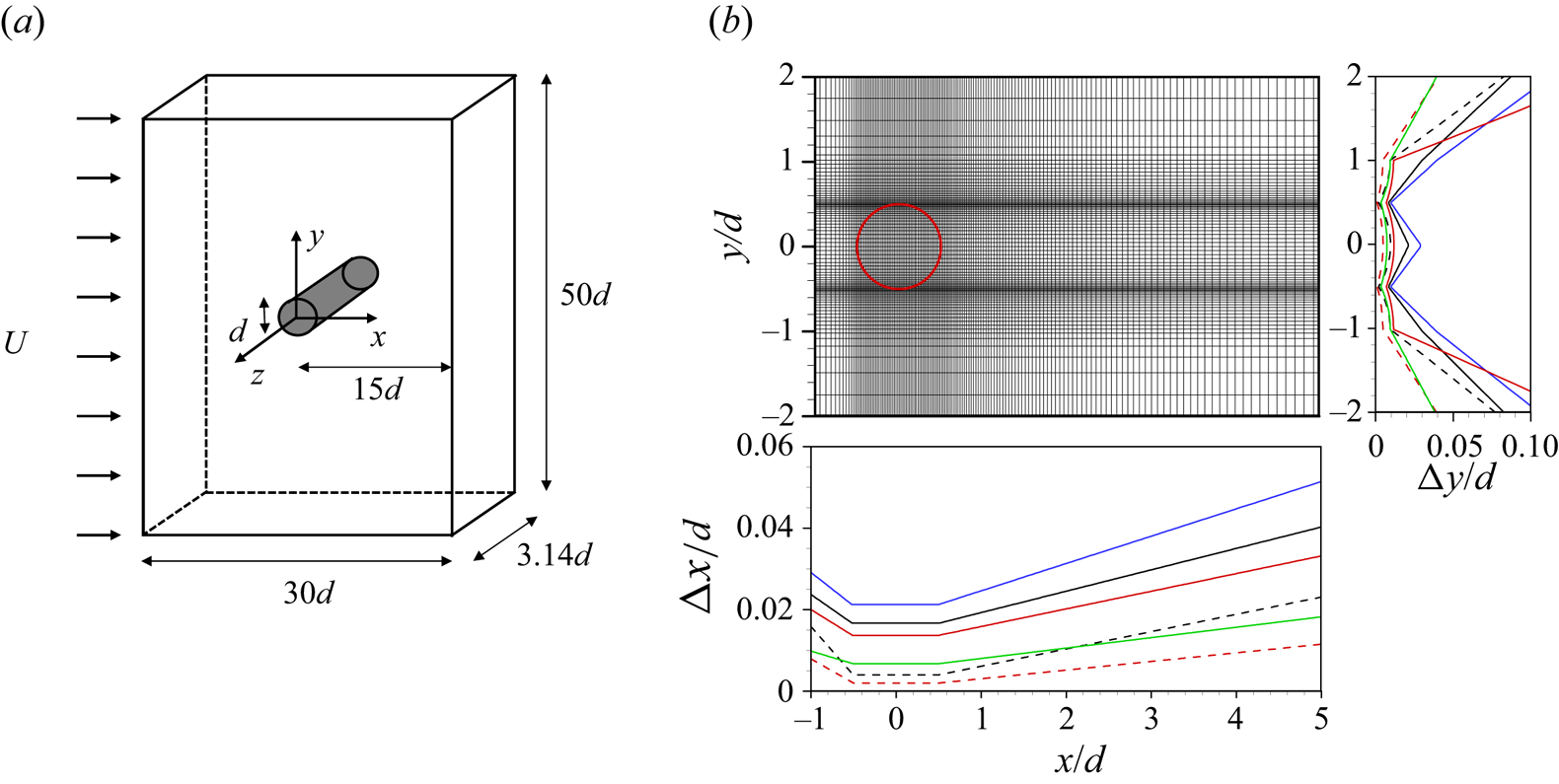
  $\tau _{ij}=0$) are solved using the second-order central difference scheme for all the spatial derivative terms on a staggered mesh, and a fractional step method with third-order Runge–Kutta and second-order Crank–Nicolson methods for the convection and diffusion terms, respectively. A computational domain and coordinate system are shown in figure 1(a), where the cylinder centre is located at $(x,y) = (0,0)$. The size of the computational domain is $L_x \times L_y \times L_z = 30d \times 50d \times 3.14d$. Note that this spanwise domain size has been adopted for DNS and LES by many previous studies (Beaudan & Moin Reference Beaudan and Moin1994; Mittal Reference Mittal1995; Breuer Reference Breuer1998; Kravchenko & Moin Reference Kravchenko and Moin1998; Ma, Karamanos & Karniadakis Reference Ma, Karamanos and Karniadakis2000; Franke & Frank Reference Franke and Frank2002; Dong et al. Reference Dong, Karniadakis, Ekmekci and Rockwell2006; Park et al. Reference Park, Lee, Lee and Choi2006; Parnaudeau et al. Reference Parnaudeau, Carlier, Heitz and Lamballais2008; Mani, Moin & Wang Reference Mani, Moin and Wang2009; Lee Reference Lee2010; Lehmkuhl et al. Reference Lehmkuhl, Rodríguez, Borrell and Oliva2013; Li et al. Reference Li, Yang, Zhang, He, Deng and Shen2020) and provides fully three-dimensional vortical structures in the wake (see, for example, figure 11). Moreover, the spanwise energy spectra fall off more than three decades at high spanwise wavenumbers (not shown here). A Dirichlet condition is used at the inlet, and a convective boundary condition, $\partial u_i / \partial t + c \partial u_i / \partial x = 0$, is used at the exit, where $c$ is the plane-averaged streamwise velocity at the exit. The Neumann condition ( $\partial u / \partial y = \partial w / \partial y = 0, v = 0$) is used at the far-field boundary, and the periodic condition is imposed in the spanwise direction. A no-slip boundary condition on the cylinder surface is satisfied with an immersed boundary method (Kim et al. Reference Kim, Kim and Choi2001). The number of grid points for DNS is $N_x\times N_y\times N_z=1025\times 501\times 128$. The grids are uniformly distributed in $z$ direction ( $\Delta z = 0.02453d$) and non-uniformly distributed in $x$ and $y$ directions, respectively, and they are densely allocated near the cylinder surface and separating shear layer region (figure 1b): e.g. the smallest grid sizes are $\Delta x_{min} = 0.004d$ and $\Delta y_{min} = 0.002d$, respectively.
Computational domain, coordinate system and grid distributions for DNS and LES: (a) computational domain and coordinate system; (b) grid distributions near the circular cylinder. In (b), ‐‐‐‐ (black), DNS3900; ‐‐‐‐ (red), DNS5000; —— (black), LES3900; —— (blue), LES3900c; —— (red), LES3900f and LES5000; —— (green), LES10000.
The data from the present DNS are validated by comparing them with those from the previous experiment (Parnaudeau et al. Reference Parnaudeau, Carlier, Heitz and Lamballais2008) and DNS (Ma et al. Reference Ma, Karamanos and Karniadakis2000). Figure 2 shows the transverse profiles of the mean streamwise velocity and r.m.s. streamwise velocity fluctuations at three streamwise locations in the wake ( $x/d=1.06$, $1.54$ and $2.02$), respectively. As shown, the present results are in excellent agreements with those of previous experiment and DNS, indicating that the choices of grids and computational domain for DNS are appropriate.
Turbulence statistics from DNS ( $Re_d = 3900$): (a) mean streamwise velocity; (b) r.m.s. streamwise velocity fluctuations. —— (red), Present DNS; $\bullet$, experiment (Parnaudeau et al. Reference Parnaudeau, Carlier, Heitz and Lamballais2008); —— (blue), DNS (Ma et al. Reference Ma, Karamanos and Karniadakis2000). Here, the bracket $\langle {\cdot } \rangle$ denotes the averaging over the spanwise direction and in time.

To estimate the prediction capabilities of the FCNN-based SGS models at untrained Reynolds numbers, another DNS is performed at  $Re_d=5000$. The computational domain size and boundary conditions are the same as those of $Re_d=3900$, as described previously. We consider three different grid distributions for the convergence of solution: $(N_x, N_y, N_z) = (2049, 1001, 128)$, $(2049, 1001, 192)$ and $(3073, 1281, 128)$, respectively. The second simulation has 1.5 times as many grid points in the spanwise direction as the first, and the third simulation uses about 1.5 times and 1.3 times as many grid points in $x$ and $y$ directions as the first, respectively (see table 1). The results from these three simulations at $Re_d=5000$ are compared with those from previous experiment and DNS in table 1 and figure 3. As shown, the results from three simulations are very similar among themselves, demonstrating the grid convergence of the present DNS. Although the mean streamwise velocity and r.m.s. streamwise velocity fluctuations along the centreline from the DNSs and experiment show some differences at $x/d < 2$ (within recirculation zone), they overall agree very well with those from the previous experiments (Norberg Reference Norberg1993, Reference Norberg1994, Reference Norberg1998), validating the accuracy of the present DNS.
Flow quantities at  $Re_d=5000$ from present DNSs, together with those from previous experiments and DNS. Here, $L_r$ is the mean recirculation length measured from the base point of the cylinder, $\langle C_{p_b} \rangle$ is the mean base pressure coefficient, $U_{min}$ is the maximum mean negative velocity along the centreline and $\langle C_D \rangle$ is the mean drag coefficient.
 $^a$Norberg (Reference Norberg1993). $^b$Norberg (Reference Norberg1994). $^c$Norberg (Reference Norberg1998). $^d$Aljure et al. (Reference Aljure, Lehmkhul, Rodríguez and Oliva2017).
Turbulence statistics from present DNSs ( $Re_d=5000$): (a) mean streamwise velocity along the centreline; (b) r.m.s. streamwise velocity fluctuations along the centreline; (c) mean streamwise velocity in the wake; (d) r.m.s. streamwise velocity fluctuations in the wake. Present DNSs (—— (red), $N_x\times N_y\times N_z = 2049 \times 1001 \times 128$; $\bullet$ (red), $2049 \times 1001 \times 192$; + (red), $3073 \times 1281 \times 128$); $\bullet$ (black), experiment (Norberg Reference Norberg1998); —— (blue), DNS (Aljure et al. Reference Aljure, Lehmkhul, Rodríguez and Oliva2017).

LESs of turbulent flow over a circular cylinder are performed at  $Re_d = 3900$, $5000$ and 10 000, respectively, with the FCNN-based SGS models developed during the present study and DSM. Numerical methods for solving the filtered continuity and Navier–Stokes equations ((2.1) and (2.2)) are the same as those of DNS. The second-order finite difference method applied to all the spatial derivative terms on a staggered mesh conserves kinetic energy as well as continuity and momentum, and does not exhibit numerical dissipation. These features make the scheme suitable for use in LES, and various complex flows have been successfully simulated using it (Mittal & Moin Reference Mittal and Moin1997). During simulation, kinetic energy is dissipated by viscous and SGS dissipation. LES without SGS dissipation can be stable when viscous dissipation alone is sufficient to maintain stability, but provides an inaccurate result. However, it becomes unstable on very coarse grids due to lack of dissipation. For DSM, a box filter of $\tilde {\varDelta }_z=2\bar {\varDelta }_z$ is used as the test filter, where $\bar {\varDelta }_z$ is the grid size in the homogeneous direction ( $z$). The domain size for LES is the same as that for DNS, but the number of grid points for LES at $Re_d = 3900$ is $N_x\times N_y\times N_z = 449\times 271\times 64$ (same number of grid points used in Lee Reference Lee2010) whose resolution is the same as that of training data. We also conduct LESs with coarser and finer grid resolutions at $Re_d = 3900$, respectively. For $Re_d = 5000$ and 10 000, we use finer grid resolutions (see table 3 later in this paper). The present computations are performed at the computational time steps of $\Delta t U/d = 0.004$, $0.003$ and $0.0025$ for $Re_d = 3900$, $5000$ and 10 000, respectively. After reaching a statistically equilibrium state, the turbulence statistics at these Reynolds numbers are obtained by averaging over $T U/d = 200$, $150$ and $125$, respectively.
2.2. Training data
As shown in Park & Choi (Reference Park and Choi2021), an FCNN trained with two databases obtained from two different grid sets predicted turbulent channel flow in LES better than an FCNN trained with a database obtained from one grid set, when LES is performed with a grid set different from those used for training. In the present study, we do not pursue the same approach as done in Park & Choi (Reference Park and Choi2021). We rather construct a database obtained with a grid set, apply a test filter having a wider filter width to it to create another database having coarser grid resolution, and train an FCNN with these two databases. Using this approach, one can certainly reduce the effort of constructing databases for training. As shown later (§ 4.2), this approach successfully predicts the flow over a circular cylinder even if the grid distribution is different from that used for training. In Appendix D, we also show the result for turbulent channel flow.
Let us apply two filters ( $\bar {G}$ and $\tilde {G}$, called grid and test filters, respectively) to a flow variable ( $f$) obtained by DNS, and calculate two filtered DNS (fDNS) variables ( $\bar {f}$ and $\tilde {f}$) as follows:
 \begin{gather} \bar{f}(x)=\int f(x')\bar{G}(x,x')\,{{\rm d}x}', \end{gather}
 \begin{gather}\tilde{f}(x)=\int f(x')\tilde{G}(x,x')\,{{\rm d}x}', \end{gather}
where  $G(x,x')$ and $\tilde {G}(x,x')$ are box filter kernels, a type of filter applicable to flow over a complex geometry. With the box filter applied in all the ( $x, y, z$) directions, the grid-filtered flow variable $\bar {f}$ is obtained as
 \begin{equation} \bar{f}(x,y,z,t)=\frac{1}{\bar{\varDelta}_x\bar{\varDelta}_y\bar{\varDelta}_z} \int_{{-}0.5\bar{\varDelta}_z}^{0.5\bar{\varDelta}_z} \int_{{-}0.5\bar{\varDelta}_y}^{0.5\bar{\varDelta}_y} \int_{{-}0.5\bar{\varDelta}_x}^{0.5\bar{\varDelta}_x} f(x+x', y+y', z+z', t) \,{{\rm d}x}' \,{{\rm d}y}' \,{\rm d}z', \end{equation}
where  $\bar {\varDelta }_{i}$ (the grid size of LES) is the filter size in $i$ direction. A one-sided box filter is used near the cylinder surface. The test-filtered flow variable $\tilde {\bar {f}}$ is obtained by applying the box filter (applied only in the spanwise direction) to the grid-filtered variable $\bar {f}$ as
 \begin{equation} \tilde{\bar{f}}(x,y,z,t)=\frac{1}{\tilde{\varDelta}_z} \int_{{-}0.5\tilde{\varDelta}_z}^{0.5\tilde{\varDelta}_z} \bar{f}(x, y, z+z', t)\,{\rm d}z', \end{equation}
where  $\tilde {\varDelta }_z ({>}\bar{\Delta}_z)$ is the size of test filter in $z$ direction. With the operations of (2.5) and (2.6), training data (i.e. grid- and test-fDNS data) are obtained. The training data are extracted from 25 instantaneous fDNS fields during approximately 20 vortex shedding cycles ( $TU/d \approx 100$; see figure 4a). Adding more instantaneous fDNS fields does not improve the prediction performance (see Appendix A for the details). From each instantaneous flow field, the fDNS data on $(x,y)$ planes at four different spanwise locations (only $278 \times 158$ grid points per plane within a dashed box in figure 4b) are taken as the training data to filter out highly correlated data. Thus, the total number of training data is $N_{tot} = 25 \times N_{xy} \times 4 = 4\,078\,400$, where $N_{xy} (=40\,784)$ is the number of grid points within the dashed box except for those inside a circular cylinder. The region close to the cylinder surface denoted as the dashed box ( $-1 \leq x/d \leq 6$ and $-1.5 \leq y/d \leq 1.5$) contains laminar and turbulent flows, and the representative flow phenomena such as the boundary layer development, flow separation, shear layer roll-up and turbulent wake. We also increase the size of the dashed box to $-1 \leq x/d \leq 8$ and $-2 \leq y/d \leq 2$, but a posteriori test provides only few changes in the LES results (see Appendix A for the details).
Spatiotemporal extraction of the training data: (a) time histories of the drag and lift coefficients (DNS); (b) contours of the instantaneous SGS shear stress  $\tau _{xy}$. In (b), the dashed box denotes the $(x,y)$ plane where training data are extracted.

3. FCNN training
3.1. Input and output variables
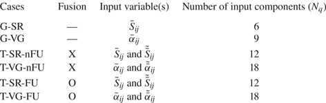
The present FCNNs (denoted as NNs hereafter) use four different input variables to predict the six components of the SGS stress tensor  $\tau _{ij}$, as listed in table 2. The grid-filtered variables are used as inputs for all NNs, whereas the test-filtered variables are used as inputs only for the cases of T-SR and T-VG. The input variables for the cases of G-SR and G-VG are the six components of the SR tensor ( $\bar {S}_{ij}=0.5({\partial \bar {u}_i}/{\partial x_j}+{\partial \bar {u}_j}/{\partial x_i})$) and nine components of the VG tensor ( $\bar {\alpha }_{ij}={\partial \bar {u}_i}/{\partial x_j}$) at each input grid point, respectively, and the output variable is the six components of $\tau _{ij}$ at the same grid point. The choice of these input variables comes from the previous NN-based LES of turbulent channel flow by Park & Choi (Reference Park and Choi2021), in which the SGS models with the inputs of $\bar {S}_{ij}$ and $\bar {\alpha }_{ij}$ were used and provided good prediction performances.
Model architectures and input variables for NNs.
For the cases of T-SR and T-VG, both the grid- and test-filtered variables are used as the input variables. The use of test-filtered variables or similar as an input to NN is not the first time. Xie et al. (Reference Xie, Wang, Li, Wan and Chen2020a) used the first-order derivatives of the grid- and test-filtered velocity and temperature at multiple grid points as inputs for compressible isotropic turbulence, and showed that their predictions of the velocity and temperature spectra were better than those by the DMM. Park & Choi (Reference Park and Choi2021) trained an NN with input variables from fDNS datasets obtained from two different filter widths, and showed that its prediction for turbulent channel flow was better than that from single fDNS dataset when an actual LES was performed with a grid resolution different from that used for training. Therefore, the addition of the test-filtered variables to the input should enhance the prediction capability of NN-based SGS models, especially when the grid resolution for LES is different from that used for training.
3.2. Neural network architectures
Most of the previous studies have adopted simple NN architectures having consecutive layers with multiple nodes (see, for example, Sarghini, de Felice & Santini Reference Sarghini, de Felice and Santini2003; Wollblad & Davidson Reference Wollblad and Davidson2008; Gamahara & Hattori Reference Gamahara and Hattori2017; Pal Reference Pal2019; Xie et al. Reference Xie, Wang, Li, Wan and Chen2020a,Reference Xie, Wang and Weinanb,Reference Xie, Yuan and Wangc; Yuan et al. Reference Yuan, Xie and Wang2020; Park & Choi Reference Park and Choi2021; Stoffer et al. Reference Stoffer, van Leeuwen, Podareanu, Codreanu, Veerman, Janssens, Hartogensis and van Heerwaarden2021; Subel et al. Reference Subel, Chattopadhyay, Guan and Hassanzadeh2021; Wang et al. Reference Wang, Yuan, Xie and Wang2021; Kang et al. Reference Kang, Jeon and You2023), as shown in figure 5(a). Park & Choi (Reference Park and Choi2021) used an NN with two hidden layers and 128 nodes per hidden layer by setting  $\bar {S}_{ij}$ or $\bar {\alpha }_{ij}$ as the input and $\tau _{ij}$ as the output, respectively, and showed its better performance than that of DSM for turbulent channel flow. However, when the grid resolution of LES was different from that of training data, the trained SGS model could not accurately predict turbulence statistics. This problem was overcome by training an SGS model with data obtained from multiple filter widths, but its performance can be degraded when the grid sizes used for LES are out of the range of training grid sizes. We use the same NN architecture (denoted as nFU architecture), and test for the present flow over a circular cylinder with grid resolutions different from the training one, resulting in similar degradation of the prediction performance (see § 4.2.2). We also increase the numbers of the hidden layers and nodes to 3 and 256, respectively, but these increases do not improve the prediction performances (see Appendix B for the details).
Schematic diagrams of the present NNs: (a) NN with two hidden layers (denoted as nFU architecture); (b) NN with two and one hidden layers before and after fusion (subtraction), respectively (denoted as FU architecture). Here,  $\bar {\boldsymbol {q}}$ and $\tilde {\bar {\boldsymbol {q}}}$ are the grid- and test-filtered inputs, respectively, $N_q$ is the number of input components (see table 2), and $\boldsymbol {s}$ is the output.

Karpathy et al. (Reference Karpathy, Toderici, Shetty, Leung, Sukthankar and Fei-Fei2014) suggested three types of fusion (early fusion, late fusion and slow fusion) to classify a video having spatiotemporal features. In that study, with shared CNN parameters, spatial features from multiple contiguous frames in time were extracted, and then the extracted features were combined by fusion. Analogous to the video classification, one may construct an NN architecture by combining extracted features from inputs with different grid resolutions by fusion. Motivated by this approach, we build a new NN architecture (denoted as FU architecture; figure 5b) by introducing additional test-filtered variables and fusing information from two separate single-frame networks. Among the three types of fusion, we adopt late fusion to consider not only the grid- and test-filtered input variables but also their difference. The present FU architecture consists of two and one hidden layers before and after fusion, respectively, and 64 nodes per hidden layer (see § 3.3). This fusion process is also motivated by the dynamic procedure of DSM (Germano et al. Reference Germano, Piomelli, Moin and Cabot1991; Lilly Reference Lilly1992). In DSM, the SGS stresses at the grid and test filter levels,  $\tau _{ij}$ and $T_{ij}$, are parameterised with the same functional form, and the resolved turbulent stress, $\mathcal {L}_{ij} = T_{ij} - \tilde {\tau }_{ij}$, is calculated explicitly. The resolved turbulent stress represents the contribution to the Reynolds stress from the length scales between the grid and test filter widths. Therefore, we expect that fusion in the FU architecture should be able to properly treat the resolved turbulent stress from the grid- and test-filtered variables, and thus enable to produce more accurate SGS stresses.
3.3. Training details
In the nFU architecture (no fusion), the output of the  $m$th layer, $\boldsymbol {h}^{(m)}$, is given as
 \begin{equation} \left. \begin{array}{l@{}}
h_i^{(1)}= \overline{q_i} \quad (i=1,2,\ldots,N_q);\\ h_j^{(2)}=\max\left[0,\gamma_j^{(2)}
\left.\left(\displaystyle\sum_{i=1}^{N_q}
W_{ij}^{(1)(2)}h_i^{(1)}+b_j^{(2)}-
\mu_j^{(2)}\right)\right/{\sigma_j^{(2)}+\beta_j^{(2)}}\right]
\\ \qquad\qquad(j=1,2,\ldots,128); \\
h_k^{(3)}=\max\left[0,\gamma_k^{(3)}\left.\left(\displaystyle\sum_{j=1}^{128}
W_{jk}^{(2)(3)}h_j^{(2)}+b_k^{(3)}-\mu_k^{(3)}
\right)\right/{\sigma_k^{(3)}+\beta_k^{(3)}}\right]
\\ \qquad\qquad(k=1,2,\ldots,128);\\
h_l^{(4)}=s_l=
\displaystyle\sum_{k=1}^{128}W_{kl}^{(3)(4)}h_k^{(3)}+b_l^{(4)}
\quad(l=1,2,\ldots,6), \end{array}\right\}
\end{equation}
\begin{equation} \left. \begin{array}{l@{}}
h_i^{(1)}= \overline{q_i} \quad (i=1,2,\ldots,N_q);\\ h_j^{(2)}=\max\left[0,\gamma_j^{(2)}
\left.\left(\displaystyle\sum_{i=1}^{N_q}
W_{ij}^{(1)(2)}h_i^{(1)}+b_j^{(2)}-
\mu_j^{(2)}\right)\right/{\sigma_j^{(2)}+\beta_j^{(2)}}\right]
\\ \qquad\qquad(j=1,2,\ldots,128); \\
h_k^{(3)}=\max\left[0,\gamma_k^{(3)}\left.\left(\displaystyle\sum_{j=1}^{128}
W_{jk}^{(2)(3)}h_j^{(2)}+b_k^{(3)}-\mu_k^{(3)}
\right)\right/{\sigma_k^{(3)}+\beta_k^{(3)}}\right]
\\ \qquad\qquad(k=1,2,\ldots,128);\\
h_l^{(4)}=s_l=
\displaystyle\sum_{k=1}^{128}W_{kl}^{(3)(4)}h_k^{(3)}+b_l^{(4)}
\quad(l=1,2,\ldots,6), \end{array}\right\}
\end{equation}
where  $\bar {\boldsymbol {q}}$ is the grid-filtered input, $N_q$ is the number of the inputs, $\boldsymbol {W}^{(m)(m+1)}$ is the weight matrix between $m$th and $(m+1)$th layers, $\boldsymbol {b}^{(m)}$ is the bias of the $m$th layer, $\boldsymbol {s}$ is the output and $\boldsymbol{\mu}^{(m)}$, $\boldsymbol {\sigma }^{(m)}$, $\boldsymbol {\gamma }^{(m)}$ and $\boldsymbol {\beta }^{(m)}$ are the parameters for a batch normalisation (Ioffe & Szegedy Reference Ioffe and Szegedy2015). A rectified linear unit (ReLu; Nair & Hinton Reference Nair and Hinton2010) is used as an activation function, and mean-squared error (MSE) is used as a loss function defined as
 \begin{equation} L=\frac{1}{2N_{xy}}\frac{1}{6}\displaystyle\sum_{l=1}^{6}\sum_{n=1}^{N_{xy}} \left(s_{l,n}^{\textrm{{fDNS}}}-s_{l,n} \right)^2, \end{equation}
where  $\boldsymbol {s}^{\textrm {{fDNS}}}$ is the SGS stress tensor obtained from fDNS data, and $N_{xy} (=40\,784$; see § 2.2) is the size of the batch.
Similarly, in the FU architecture (with fusion), the output of the  $m$th layer, $\boldsymbol {h}^{(m)}$, is as follows:
 \begin{equation} \left. \begin{array}{l} h_{1i}^{(1)}=\overline{q_i} \quad (i=1,2,\ldots,N_q/2);\\[3pt] h_{2i}^{(1)}=\widetilde{\overline{q_i}} \quad (i=1,2,\ldots,N_q/2);\\[3pt] h_{1j}^{(2)}=\max\left[0,\gamma_{1j}^{(2)}\left.\left(\displaystyle\sum_{i=1}^{N_q/2} W_{1ij}^{(1)(2)}h_{1i}^{(1)}+b_{1j}^{(2)}-\mu_{1j}^{(2)}\right)\right/ {\sigma_{1j}^{(2)}+\beta_{1j}^{(2)}}\right] \\[4pt] \qquad\qquad (j=1,2,\ldots,64);\\[9pt] h_{2j}^{(2)}=\max\left[0,\gamma_{2j}^{(2)}\left.\left(\displaystyle\sum_{i=1}^{N_q/2} W_{2ij}^{(1)(2)} h_{2i}^{(1)}+b_{2j}^{(2)}-\mu_{2j}^{(2)}\right)\right/{\sigma_{2j}^{(2)}+\beta_{2j}^{(2)}}\right]\\[3pt] \qquad\qquad (j=1,2,\ldots,64);\\[9pt] h_{1k}^{(3)}=\max\left[0,\gamma_{1k}^{(3)}\left.\left(\displaystyle\sum_{j=1}^{64} W_{1jk}^{(2)(3)} h_{1j}^{(2)}+b_{1k}^{(3)}-\mu_{1k}^{(3)}\right)\right/{\sigma_{1k}^{(3)}+\beta_{1k}^{(3)}}\right]\\[3pt] \qquad\qquad (k=1,2,\ldots,64);\\[4pt] h_{2k}^{(3)}=\max\left[0,\gamma_{2k}^{(3)}\left.\left(\displaystyle\sum_{j=1}^{64} W_{2jk}^{(2)(3)} h_{2j}^{(2)}+b_{2k}^{(3)}-\mu_{2k}^{(3)}\right)\right/{\sigma_{2k}^{(3)}+\beta_{2k}^{(3)}}\right]\\[3pt] \qquad \qquad (k=1,2,\ldots,64);\\[9pt] h_k^{(4)}=h_{1k}^{(3)}-h_{2k}^{(3)} \quad (k=1,2,\ldots,64);\\[9pt] h_l^{(5)}=s_l=\displaystyle\sum_{k=1}^{64}W_{kl}^{(4)(5)}h_k^{(4)}+b_{l}^{(5)}\quad (l=1,2,\ldots,6),\\ \end{array}\right\} \end{equation}
where  $\bar {\boldsymbol {q}}$ and $\tilde {\bar {\boldsymbol {q}}}$ are the grid- and test-filtered inputs, respectively, $\boldsymbol {h}^{(4)}$ is from fusion (Karpathy et al. Reference Karpathy, Toderici, Shetty, Leung, Sukthankar and Fei-Fei2014), and other parameters are the same as those in the nFU architecture. A stochastic gradient descent with a learning rate of 0.01 is used to optimise the trainable parameters, and the weight and bias are initialised by using Xavier (Glorot & Bengio Reference Glorot and Bengio2010) and zero initialisations, respectively. Training and validation data are extracted from 25 and 7 instantaneous fields, respectively (approximately 75 % of instantaneous fields for training and 25 % for validation). With these databases, the NNs are trained, and training is stopped to avoid overfitting if the validation loss increases. Both nFU and FU architectures are trained by using the Python open-source library, TensorFlow.
While training the NNs, the input and output variables are normalised by the free-stream velocity  $U$ and cylinder diameter $d$. In turbulent channel flow, Park & Choi (Reference Park and Choi2021) used the input and output variables in wall units, and showed that the SGS model has an excellent prediction performance not only at the trained Reynolds number but also at a higher Reynolds number when the grid resolutions in wall units are the same. However, for the present flow, the wall unit is not proper for normalisation because it contains turbulent wake behind the cylinder surface. We also consider the normalisation of flow variables with the mean and r.m.s. values, such as $\tau _{ij}^{*}(x,y,z,t)=(\tau _{ij}(x,y,z,t)-\tau _{ij}^{mean}(x,y))/\tau _{ij}^{rms}(x,y)$, to scale the input and output variables with zero mean and unit variance. Although this normalisation may be good for training the architecture, it requires a priori knowledge about the mean and r.m.s. values for untrained Reynolds number flow. Thus, we normalise the input and output variables with $U$ and $d$.
$d$.
4. Results
In § 4.1, we perform a priori tests at  $Re_d=3900$ and 5000 with the nFU and FU architectures that are trained with the fDNS data at $Re_d=3900$. The SGS shear stress, SGS dissipation and backward SGS dissipation obtained by the trained architectures are compared with those of fDNS and DSM. In § 4.2.1, a posteriori tests (i.e. actual LESs) are conducted at $Re_d = 3900$ with the same grid resolution as that of the trained fDNS data. These LES results are compared with those of fDNS and from LESs with DSM and without SGS model, respectively. In § 4.2.2, we perform LESs at $Re_d=3900$ with grid resolutions different from that of the trained fDNS data, and discuss the results. Finally, in § 4.2.3, LESs are carried out at $Re_d=5000$ and 10 000, and their results are compared with those of fDNS and previous experiment.
4.1. A priori tests
A priori tests at  $Re_d=3900$ and 5000 are conducted with the nFU and FU architectures trained at $Re_d=3900$. We do not conduct a priori test for $Re_d=10\,000$, because the fDNS data at this Reynolds number are not available at hand. Figure 6 shows the profiles of the mean SGS shear stress $\langle \tau _{xy}\rangle$, mean SGS dissipation $\langle \epsilon _{SGS}\rangle$ and mean backward SGS dissipation $\langle \epsilon ^-_{SGS}\rangle$ (backscatter) at $x/d = 1.06$, $1.54$ and 2.02 for $Re_d = 3900$ and 5000, respectively, where $\epsilon _{SGS}=-\tau _{ij}\bar {S}_{ij}$ and $\langle \epsilon ^-_{SGS}\rangle =\frac {1}{2}\langle \epsilon _{SGS}-|\epsilon _{SGS}|\rangle$. Also shown in figure 6 are those of fDNS and from DSM.
Statistics of the SGS variables at three streamwise locations in the wake from a priori tests ( $Re_d=3900$ (left) and 5000 (right)): (a) mean SGS shear stress $\langle\tau_{xy}\rangle$; (b) mean SGS dissipation $\langle\epsilon_{SGS}\rangle$; (c) mean backscatter $\langle\epsilon^-_{SGS}\rangle$. $\bullet$, fDNS; —— (blue), G-SR; ‐‐‐‐ (blue), G-VG; —— (green), T-SR-nFU; ‐‐‐‐ (green), T-VG-nFU; —— (red), T-SR-FU; ‐‐‐‐ (red), T-VG-FU; $+$, DSM.

At  $x/d=1.06$, G-SR and G-VG, and T-SR-FU and T-VG-FU, respectively, show similar predictions of $\langle \tau _{xy}\rangle$ and $\langle \epsilon _{SGS}\rangle$. However, the SGS shear stresses from T-SR-nFU and T-VG-nFU have negative and positive peaks in the lower and upper shear layer regions for $Re_d = 3900$, respectively, which is opposite to that of fDNS data. A similar behaviour is observed for the SGS dissipation. The backscatter profiles ( $\langle \epsilon ^-_{SGS}\rangle$) from G-SR, G-VG, T-SR-nFU and T-VG-nFU contain high peaks in the upper and lower shear layer regions unlike that of fDNS data, but those from T-SR-FU and T-VG-FU are underpredicted but similar to that of fDNS. On the other hand, at $x/d=1.54$ and 2.02, G-SR, T-SR-nFU and T-SR-FU (input of $\bar {S}_{ij}$), and G-VG, T-VG-nFU and T-VG-FU (input of $\bar {\alpha }_{ij}$) show similar performances, respectively, regardless of using fusion. The predictions from all the architectures are better than that from DSM (note that the backscatter from DSM is zero). The architectures with the input of $\bar {\alpha }_{ij}$ predict these statistics better than those with the input of $\bar {S}_{ij}$. However, as is well known from the studies of the traditional and NN-based SGS modelling (Park et al. Reference Park, Lee, Lee and Choi2006; Gamahara & Hattori Reference Gamahara and Hattori2017; Beck et al. Reference Beck, Flad and Munz2019; Park & Choi Reference Park and Choi2021), a better prediction in a priori test does not guarantee a better performance in a posteriori test (i.e. actual LES).
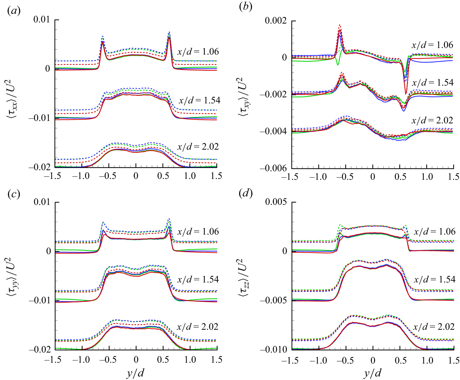
As discussed in Duraisamy (Reference Duraisamy2021), one of the reasons for this inconsistency between a priori and a posteriori tests is that errors are accumulated over time and, thus, resolved scales are corrupted. Hence, we take another a priori test to assess the robustness of the NN-based SGS models. The robustness is one of the indices that can represent the sensitivity of the NNs, defined as the degree to which a system or component can function correctly in the presence of invalid inputs or stressful environmental conditions (IEEE 1990). Thus, we add noise to the present inputs ( $\bar {S}_{ij}$ and $\tilde {\bar {S}}_{ij}$) and observe how outputs ( $\tau _{ij}$) are changed for the present NN-based SGS models. Let us define $\bar {\sigma }_{ij}$ and $\tilde {\bar {\sigma }}_{ij}$ as the standard deviations of the inputs ( $\bar {S}_{ij}$ and $\tilde {\bar {S}}_{ij}$) in the training databases, respectively. Then, the random inputs are added as follows (Ferri, Hernández-Orallo & Modroiu Reference Ferri, Hernández-Orallo and Modroiu2009; Fabra-Boluda et al. Reference Fabra-Boluda, Ferri, Martínez-Plumed and Ramírez-Quintana2022):
 \begin{equation} \left.\begin{gathered} \bar{S}'_{ij} = \bar{S}_{ij} + N(0, \bar{\sigma}^2_{ij}),\\ \tilde{\bar{S}}'_{ij} = \tilde{\bar{S}}_{ij} + N(0, \tilde{\bar{\sigma}}^2_{ij}), \end{gathered}\right\} \end{equation}
where  $N(0, \sigma ^2)$ is the normal distribution with zero mean and standard deviation of $\sigma$. We consider G-SR, T-SR-nFU and T-SR-FU for assessing their robustness, and results are shown in figure 7. The changes in the normal and shear SGS stresses ( $\tau _{xx}$, $\tau _{yy}$ and $\tau _{xy}$) are bigger for G-SR and T-SR-nFU than those for T-SR-FU, whereas the changes in $\tau _{zz}$ are relatively insensitive to the models except the shear layer region at $x/d = 1.06$ for T-SR-nFU. This result indicates that T-SR-FU is the most robust among these models. Therefore, we expect better performance from a posteriori test with T-SR-FU (see the following).
Robustness of the NN-based SGS models under the inputs without and with noise (equation 4.1) ( $Re_d=3900$): (a) $\langle\tau_{xx}\rangle$; (b) $\langle\tau_{xy}\rangle$; (c) $\langle\tau_{yy}\rangle$; (d) $\langle\tau_{zz}\rangle$. —— (blue), G-SR without noise; ‐‐‐‐ (blue), G-SR with noise; —— (green), T-SR-nFU without noise; ‐‐‐‐ (green), T-SR-nFU with noise; —— (red), T-SR-FU without noise; ‐‐‐‐ (red), T-SR-FU with noise.
4.2. A posteriori tests
A posteriori tests (actual LESs) are conducted for flow over a circular cylinder at  $Re_d=3900$, 5000 and 10 000 with the NN-based SGS models trained at $Re_d = 3900$. The computational domain size is fixed to be $30d \times 50d \times 3.14d$ for all cases. Table 3 summarises the computational parameters for LESs and flow parameters obtained from LESs with various SGS models, together with those of DNS, DSM and no SGS model. Note that, in LES with DSM, the model coefficient of the eddy viscosity is obtained by averaging over $z$ direction (Germano et al. Reference Germano, Piomelli, Moin and Cabot1991; Lilly Reference Lilly1992; Mittal & Moin Reference Mittal and Moin1997; Breuer Reference Breuer1998; Kravchenko & Moin Reference Kravchenko and Moin2000; Mani et al. Reference Mani, Moin and Wang2009). The grid resolution for the cases of LES3900 is the same as that of fDNS used in training SGS models, and those of LES3900c and LES3900f are coarser and finer than that of LES3900, respectively. In cases of LES5000 and LES10000, the grid resolutions are finer than that of LES3900. For $Re_d = 5000$, the numbers of grid points used for DNS and fDNS are $2049 \times 1001 \times 128$ and $545 \times 301 \times 64$, respectively, and the grid resolution for the cases of LES5000 is the same as that of fDNS. More on the grid-resolution study for a posteriori tests at $Re_d=3900$, 5000 and 10 000 is given in Appendix C.
Computational parameters for LESs and simulation results. Here,  $L_r$ is the mean recirculation length measured from the base point of the cylinder, $\langle C_{p_b} \rangle$ is the mean base pressure coefficient, $U_{min}$ is the maximum mean negative velocity along the centreline and $\langle C_D \rangle$ is the mean drag coefficient.
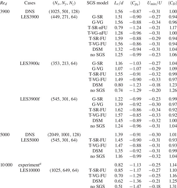
 $^a$Dong et al. (Reference Dong, Karniadakis, Ekmekci and Rockwell2006).
4.2.1. LES with the grid resolution same as that of training data ( $Re_d = 3900$)

As listed in table 3, for LES3900, the statistics from G-SR and G-VG and T-SR-FU and T-VG-FU are in good agreements with those of DNS, whereas T-SR-nFU and T-VG-nFU do not predict these statistics very well. In particular, G-SR, G-VG, T-SR-FU and T-VG-FU predict the recirculation length and base pressure coefficient more accurately than DSM does. The profiles of the mean streamwise velocity and r.m.s. streamwise velocity fluctuations at three streamwise locations in the wake from LES3900 are shown in figure 8, together with those of fDNS, DSM and no SGS model. As shown, the results from G-SR, G-VG, T-SR-FU and T-VG-FU are in excellent agreements with those of fDNS and are better than those of DSM, whereas T-SR-nFU and T-VG-nFU show poor predictions (T-SR-nFU is even worse than no SGS model). Figure 9 shows the contours of the instantaneous vorticity magnitude at a spanwise location from the present SGS models, fDNS, DSM and no SGS model, respectively. At  $Re_d = 3900$, the upper and lower shear layers are elongated downstream and very few vortical structures exist very near the base surface (see the case of fDNS in this figure). However, the contours from no SGS model are significantly distorted in the shear layer and near-wake contains full of small scales because of lack of turbulent dissipation. The cases of T-SR-nFU and T-VG-nFU show somewhat similar (but with lower vorticity magnitudes) behaviours to that of no SGS model. That is, the shear layer transition starts earlier by weak SGS dissipation that was observed in a priori test (figure 6). Therefore, when the grid resolution of a posteriori test is the same as that of training data, the grid- and test-filtered inputs with fusion as well as the grid-filtered input alone successfully predict the statistics, while the grid- and test-filtered inputs without fusion do not accurately predict the turbulence statistics. Note that this result is consistent with the a priori result of $\tau _{xy}$ near the shear layer from T-SR(VG)-nFU. Hence, the grid-filtered input alone is sufficient to produce successful predictions when the trained NN is applied to a a posteriori test using the same grids and, thus, additional test-filtered input to the same NN (such as T-SR-nFU and T-VG-nFU) degrades the prediction performance through lower correlations among nodes. On the other hand, when the test-filtered input is provided to a separate NN from that of the grid-filtered input, the combined NNs (such as T-SR-FU and T-VG-FU) avoid this problem and perform quite well.
Flow statistics from LES3900 (a posteriori test): (a) mean streamwise velocity; (b) r.m.s. streamwise velocity fluctuations.  $\bullet$, fDNS; —— (blue), G-SR; ‐‐‐‐ (blue), G-VG; —— (green), T-SR-nFU; ‐‐‐‐ (green), T-VG-nFU; —— (red), T-SR-FU; ‐‐‐‐ (red), T-VG-FU; +, DSM; $\circ$, no SGS model.

Contours of the instantaneous vorticity magnitude in the near-wake behind the cylinder ( $Re_d = 3900$). The contour levels are from $|\omega |d/U= 0$ to 30 by increments of 3. An inset for the case of T-SR-FU is the result of applying a hybrid scheme ( $\textrm {QUICK} + \textrm {CD}2$; Yun et al. Reference Yun, Kim and Choi2006) to the convection terms of the Navier–Stokes equations.

Note in figure 9 that spurious oscillations appear near the front surface due to the dispersive nature of second-order central difference scheme (CD2). To avoid these oscillations, one should provide much more grids in this laminar accelerating flow region. To see if these oscillations propagate downstream, a hybrid scheme (QUICK scheme at a laminar accelerating flow region ( $x/d < -0.25$) and CD2 elsewhere; Yun, Kim & Choi Reference Yun, Kim and Choi2006) is applied to the convection terms for the case of T-SR-FU, and its result is given as an inset in the result of T-SR-FU in figure 9. As shown, the flow structures from CD2 alone and from this hybrid scheme are very similar to each other except for those oscillations, indicating that they do not propagate downstream at this relatively low Reynolds number. However, for a much higher Reynolds number, a hybrid scheme may have to be used to avoid the propagation of these spurious oscillations into downstream.
4.2.2. LES with a grid resolution different from that of training data ($Re_d = 3900$)

In this section, we provide results from LES with a grid resolution different from that of training data. Due to the poor performances of T-SR-nFU and T-VG-nFU, other four NN-based SGS models are investigated. Two different grid resolutions (LES3900c and LES3900f) are considered as listed in table 3. LES3900c and LES3900f have coarser and finer grid resolutions on  $(x, y)$ planes, respectively, and have the same grid resolution in $z$ direction as that of LES3900 (more on the grid-resolution study is given in Appendix C, and computational costs for estimating the SGS stresses from G-SR and T-SR-FU are compared with that from DSM in Appendix E). For LES3900c, the prediction performances of G-SR and G-VG are significantly degraded especially for the recirculation length and base pressure coefficient. On the other hand, T-SR-FU and T-VG-FU predict these variables quite reasonably, maintaining their prediction capabilities even with coarser grid resolution used. Note that DSM with this coarse resolution predicts much smaller recirculation length, lower base pressure coefficient and higher drag coefficient. For LES3900f, the predictions with DSM are in excellent agreements with those of DNS, but those with G-SR and G-VG become closer to those of DNS but still not better than those with the same grid resolution as that of training data. It is noteworthy that the prediction performances of T-SR-FU and T-VG-FU do not become worse even when the resolution used is different from that of training data.
Figure 10 shows the profiles of the mean streamwise velocity and r.m.s. streamwise velocity fluctuations from four NN-based SGS models with coarser and finer grid resolutions (LES3900c and LES3900f, respectively) than that of training data, together with those of fDNS, DSM and no SGS model. For LES3900c, the use of fusion with grid- and test-filtered input variables (T-SR-FU and T-VG-FU) predicts  $\langle \bar {u}\rangle$ and ${\bar {u}}_{rms}$ quite accurately, whereas the grid-filtered input variables alone (G-SR and G-VG) do not accurately predict them (note, however, that the predictions are still better than those of DSM with this coarser grid resolution). When the grid resolution is finer (LES3900f) than that of training data, both T-SR-FU and T-VG-FU and DSM accurately predict these flow variables, whereas the predictions of G-SR and G-VG are not good. From the results given in table 3 and figure 10, it is clear that the grid- and test-filtered inputs are better than the grid-filtered input alone and fusion connecting these two different filtered inputs significantly increases the prediction performance, when the grid resolution used is different from that of training data. The present results clearly indicate that, by constructing multiple filtered datasets with different filter sizes and using them to train an NN with fusion, one can expect a successful NN-based LES, even if the grid resolution is different from the resolutions used to construct the NN. A similar conclusion was also made in Park & Choi (Reference Park and Choi2021). Note also that this result is consistent with that from the robustness of G-SR and T-SR-FU in § 4.1.
Flow statistics from LES3900c and LES3900f (coarser and finer grid resolutions than that of training data, respectively; a posteriori test): (a) mean streamwise velocity (LES3900c); (b) r.m.s. streamwise velocity fluctuations (LES3900c); (c) mean streamwise velocity (LES3900f); (d) r.m.s. streamwise velocity fluctuations (LES3900f).  $\bullet$, fDNS; —— (blue), G-SR; ‐‐‐‐ (blue), G-VG; —— (red), T-SR-FU; ‐‐‐‐ (red), T-VG-FU; $+$, DSM; $\circ$, no SGS model.

Sirignano et al. (Reference Sirignano, MacArt and Freund2020) evaluated the discretisation errors in LES from finite-difference schemes by comparing finite-differenced spatial derivatives of the filtered velocity on the DNS and LES grids, respectively. We follow this approach for estimating the magnitudes of discretisation errors in LES from the second-order finite difference scheme used in the present study, and provide the results in table 4. In this table,  $\langle \vert \delta \bar {\alpha }_{ij} \vert \rangle / \langle \vert \bar {\alpha }_{ij} \vert _{{\tiny DNS}} \rangle$ is the relative magnitude of discretisation error of calculating $\bar {\alpha }_{ij}$ in LES, and $\delta \bar {\alpha }_{ij}$ is obtained as
 \begin{equation} \delta \bar{\alpha}_{ij} = \bar{\alpha}_{ij}\vert_{{\tiny LES}} - \bar{\alpha}_{ij}\vert_{{\tiny DNS}},\\ \end{equation}
where
 \begin{equation} \left.\begin{gathered}
\bar{\alpha}_{ij} \vert_{{\tiny LES}} = \frac{\bar{u}_i
\left(x_j+\dfrac{1}{2}\Delta x_j \vert_{{\tiny LES}}\right) -
\bar{u}_i\left(x_j-\dfrac{1}{2}\Delta x_j \vert_{{\tiny
LES}}\right)}{\Delta x_j\vert_{{\tiny LES}}},\\ \bar{\alpha}_{ij}
\vert_{{\tiny DNS}} = \frac{\bar{u}_i
\left(x_j+\dfrac{1}{2}\Delta x_j \vert_{{\tiny DNS}}\right) -
\bar{u}_i\left(x_j-\dfrac{1}{2}\Delta x_j \vert_{{\tiny
DNS}}\right)}{\Delta x_j\vert_{{\tiny DNS}}},
\end{gathered}\right\}
\end{equation}
\begin{equation} \left.\begin{gathered}
\bar{\alpha}_{ij} \vert_{{\tiny LES}} = \frac{\bar{u}_i
\left(x_j+\dfrac{1}{2}\Delta x_j \vert_{{\tiny LES}}\right) -
\bar{u}_i\left(x_j-\dfrac{1}{2}\Delta x_j \vert_{{\tiny
LES}}\right)}{\Delta x_j\vert_{{\tiny LES}}},\\ \bar{\alpha}_{ij}
\vert_{{\tiny DNS}} = \frac{\bar{u}_i
\left(x_j+\dfrac{1}{2}\Delta x_j \vert_{{\tiny DNS}}\right) -
\bar{u}_i\left(x_j-\dfrac{1}{2}\Delta x_j \vert_{{\tiny
DNS}}\right)}{\Delta x_j\vert_{{\tiny DNS}}},
\end{gathered}\right\}
\end{equation} $\langle {\cdot } \rangle$ is the average in time and over the training zone shown in figure 4(b), and $\Delta x_j \vert _{{\tiny LES}}$ and $\Delta x_j \vert _{{\tiny DNS}}$ are the grid spacings in LES and DNS, respectively. Table 4 indicates that, for all the cases considered, $\langle \vert \delta \bar {\alpha }_{ij} \vert \rangle$ (difference between $\bar {\alpha }_{ij}$ on the DNS and LES grids) is about half the average magnitude of the VG evaluated on the DNS grids, indicating that the finite-difference errors in LES is not so significant, and the NN-based models trained may not suffer form the finite difference errors (see also Sirignano et al. (Reference Sirignano, MacArt and Freund2020) for further discussion).
Averaged relative magnitudes of finite-differencing errors, evaluated for filter sizes of  $\varDelta (\textrm {LES})/\varDelta (\textrm {DNS})=2$ (for $Re_d = 3900$, the size of LES grids in each direction is about two times that of DNS grids; see table 3). The information on LES3900cc (Gcc-64) and LES390ccc (Gccc-64) are given in table 5.

Numbers of grid points used for a posteriori test at  $Re_d = 3900$. Note that the grid distributions of G-64, Gf-64 and Gc-64 in this table are the same as those of LES3900, LES3900f and LES3900c in table 3, respectively.
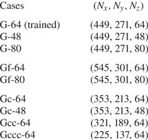
4.2.3. LES at higher Reynolds numbers ($Re_d = 5000$ and 10 000)

In this section, we perform LESs at  $Re_d = 5000$ and 10 000, which are higher than that of training data ( $Re_d = 3900$). The grid resolutions at $Re_d=5000$ and 10 000 are the same as and finer than that of LES3900f, respectively, as listed in table 3. These Reynolds numbers are selected as untrained cases, because the flows at these Reynolds numbers are quite different from the trained Reynolds number flow. In the shear layer transition regime ( $1000 < Re_d < 200\,000$), the Strouhal number, base pressure coefficient and recirculation length decrease, and the Reynolds stress increases, as the Reynolds number increases (Williamson Reference Williamson1996). These trends can be also observed in table 3. In this regime, with increasing Reynolds number, the onset of shear layer transition occurs earlier, with which the shear-layer vortices evolve earlier and the alternating Kármán vortices exist closer to the base of the cylinder (Dong et al. Reference Dong, Karniadakis, Ekmekci and Rockwell2006). These flow characteristics can be observed in figure 11, where the instantaneous vortical structures identified by the iso-surfaces of $\lambda _2=-50U^2/d^2$ (Jeong & Hussain Reference Jeong and Hussain1995) are shown together with the contours of the instantaneous pressure at $Re_d = 3900$ and 10 000, respectively. Therefore, it will be interesting to see how the NN-based SGS models trained at $Re_d = 3900$ perform at higher Reynolds numbers.
Instantaneous vortical structures coloured with the contours of the instantaneous pressure from T-SR-FU: (a)  $Re_d=3900$ (LES3900); (b) $Re_d=10\,000$ (LES10000).

Figure 12 shows the results from T-SR-FU and T-VG-FU at  $Re_d=5000$ (LES5000), together with those of fDNS, DSM and no SGS model. The grid resolution of LES5000 is the same as that of LES3900f. Similar to the results from LES3900f, T-SR-FU, T-VG-FU and DSM have excellent prediction performances. The predicted flow parameters in table 3 are also in good agreements with those of DNS.
Flow statistics from LES5000 (a posteriori test): (a) mean streamwise velocity; (b) r.m.s. streamwise velocity fluctuations.  $\bullet$, fDNS; —— (red), T-SR-FU; ‐‐‐‐ (red), T-VG-FU; $+$, DSM; $\circ$, no SGS model.

Figure 13 shows the profiles of the mean streamwise velocity and r.m.s. streamwise velocity fluctuations from LES10000, together with those of an experiment (Dong et al. Reference Dong, Karniadakis, Ekmekci and Rockwell2006), DSM and no SGS model. As shown, both T-SR-FU and T-VG-FU accurately predict those statistics (even slightly better than DSM), even though the flow at  $Re_d=10\,000$ is untrained and the transitional phenomena in the separating shear layer is notably altered. Moreover, T-SR-FU, which uses the SR as the input variable, shows slightly better predictions than T-VG-FU at this Reynolds number. The results provided in this subsection clearly indicate that both the grid- and test-filtered input variables with fusion increase the prediction capability even for untrained Reynolds number flows.
Flow statistics from LES10000 (a posteriori test): (a) mean streamwise velocity; (b) r.m.s. streamwise velocity fluctuations.  $\bullet$, experiment (Dong et al. Reference Dong, Karniadakis, Ekmekci and Rockwell2006); —— (red), T-SR-FU; ‐‐‐‐ (red), T-VG-FU; $+$, DSM; $\circ$, no SGS model.

Lastly, one may suggest combining DNS databases at  $Re = 3900$ and 5000 to widen input ranges of $\bar {\alpha }_{ij}$ and $\bar {S}_{ij}$ and improve the prediction capability. This approach should work for higher-Reynolds-number flows. Nevertheless, in the present study, we show that the present approach with a database at $Re=3900$ alone can predict the flows at higher Reynolds numbers.
5. Conclusions
Recently, many studies have been performed to develop NN-based SGS models for LES. However, most of them have focused on simple turbulent flows such as isotropic turbulence and turbulent channel flow, and an application to complex flow is very limited. Since NN-based SGS models should be eventually applied to any complex flows, it is important to develop such models and test them for representative complex flows. Therefore, in the present study, we chose a circular cylinder as a representative complex flow. We believe that the present study may be one of the first attempts to develop and apply NN-based SGS models to a complex flow.
In the present study, FCNNs were constructed to develop SGS models that predicted the SGS stresses for flow over a circular cylinder, and a priori and a posteriori tests were conducted to estimate their prediction performances. To obtain SGS models, we proposed a new FCNN architecture that used both grid- and test-filtered variables as inputs and fusion connecting these two different inputs, and compared its prediction performance with that of an FCNN architecture that had only the grid-filtered variable as input. As the input variable, the SR or VG tensor at a single grid point was considered. Hence, we constructed six different FCNN-based SGS models: G-SR and G-VG (grid-filtered SR and VG as the input variables, respectively), T-SR-nFU and T-VG-nFU (grid- and test-filtered SR and VG as the input variables, respectively, without fusion) and T-SR-FU and T-VG-FU (grid- and test-filtered SR and VG as the input variables, respectively, with fusion).
For training database, fDNS data were obtained by applying the box filter to the DNS data at  $Re_d=3900$. The training data were extracted from 25 instantaneous fDNS fields during approximately 20 vortex shedding cycles, and the fDNS data from $(x,y)$ planes at four different spanwise locations were used for the training data. The FCNN architectures were trained with these training data to generate six SGS models, and a priori and a posteriori tests were conducted for the comparison of their prediction performances.
In a priori tests, the FCNN-based SGS models had better predictions of the SGS stress, SGS dissipation and backscatter than the DSM. However, the results of T-SR-nFU and T-VG-nFU showed the distributions of SGS shear stress and dissipation opposite to those of fDNS in the shear layer regions near the cylinder, and thus high peaks of backscatter were observed there. Due to the lack of dissipation in these regions, a posteriori tests showed early evolution of the shear layer instability and non-physical small-scale vortices in the near-wake region, resulting in inaccurate predictions of turbulence statistics. On the other hand, G-SR, G-VG, T-SR-FU and T-VG-FU showed better performances than DSM. These four SGS models were applied to LESs with two different grid resolutions which were coarser and finer than that of the training data. With untrained grid resolutions, T-SR-FU and T-VG-FU still showed good prediction performances, but G-SR and G-VG did not, indicating that both the grid- and test-filtered variables with fusion increased the prediction performance when the grid resolution was different from that of the training data. Finally, we applied T-SR-FU and T-VG-FU trained at  $Re = 3900$ to LESs at higher Reynolds numbers of $Re_d=5000$ and 10 000, and also obtained quite accurate turbulence statistics.
Since the present idea of combining the grid- and test-filtered input variables with fusion for constructing an FCNN architecture has not been applied to any simple flow, we apply G-SR and T-SR-FU to LES of turbulent channel flow at  $Re_\tau = 178$. As shown in Appendix D, adding the test-filtered variable as an additional input together with fusion increases the prediction accuracy for turbulent channel flow. Therefore, the present FCNN architecture with the grid- and test-filtered input variables and fusion may be applicable to other complex flows.
Lastly, the present NN-based SGS models cannot overcome a well-known limitation of traditional SGS models: inconsistency between a priori and a posteriori tests. To overcome this inconsistency, Sirignano et al. (Reference Sirignano, MacArt and Freund2020) developed an NN-based SGS model by solving adjoint partial differential equations for isotropic turbulence to match the mean filtered velocity of LES with fDNS data. In addition, Kim et al. (Reference Kim, Kim, Kim and Lee2022) developed SGS models based on deep RL for turbulent channel flow to maximise the statistical accuracy such as the mean viscous and Reynolds stresses. In contrast to the isotropic turbulence and turbulent channel flow, it should be very difficult to determine a target to match for flow over/inside a complex geometry because it is a priori unknown for those flows. On the other hand, the present NN-based SGS model may have scalability to general flows by accumulating more databases from various turbulent flows and combining those databases into one NN architecture.
Funding
This work is supported by the National Research Foundation through the Ministry of Science and ICT (number 2022R1A2B5B02001586). The computing resources are provided by the KISTI Super Computing Center (number KSC-2021-CRE-0292).
Declaration of interests
The authors report no conflict of interest.
Appendix A. Effects of the size of training data in a priori and a posteriori tests
At present, the data from 25 instantaneous fDNS fields ( $N_t = 25$) during approximately 20 vortex shedding cycles and $(x,y)$ planes at four spanwise locations ( $N_s=4$) per instantaneous field are taken as the training data. Figures 14(a) and 14(b) show the variations of the mean SGS shear stress with the changes in $N_t(=13, 25\ \textrm {and}\ 50)$ and $N_s(=2, 4\ \textrm {and}\ 8)$, respectively. As shown in this figure, the effect of varying $N_t$ and $N_s$ is very small, indicating that $N_t=25$ and $N_s=4$ are sufficient for training purpose.
Effect of the number of training data on the mean SGS shear stress (a priori test;  $Re_d = 3900$): (a) $N_t=25$ (——, black), $N_t=13$ (——, blue) and $N_t=50$ (——, red) with $N_s=4$; (b) $N_s=4$ (——, black), $N_s=2$ (——, blue) and $N_s=8$ (——, red) with $N_t=25$. $\bullet$, fDNS.

In addition, in figure 4(b), the domain size for extracting training data is  $-1 \leq x/d \leq 6$ and $-1.5 \leq y/d \leq 1.5$. We change this domain size to smaller and larger ones, respectively, and their results are given in figure 15. As shown, the present domain size is sufficient to accurately predict the mean velocity and r.m.s. velocity fluctuations, but the smaller one is too small to carry all the important velocity field information.
Effect of the domain size of extracting training data on the mean streamwise velocity and r.m.s. streamwise velocity fluctuations (a posteriori test;  $Re_d = 3900$): (a) mean streamwise velocity; (b) r.m.s. streamwise velocity fluctuations. $\bullet$, fDNS; —— (black), present domain ( $-1 \le x/d \le 6, -1.5 \le y/d \le 1.5$); —— (blue), smaller domain ( $-1 \le x/d \le 4, -1 \le y/d \le 1$); —— (red), larger domain ( $-1 \le x/d \le 8, -2 \le y/d \le 2$).

Appendix B. Effects of the numbers of the hidden layers and nodes on the flow statistics from a posteriori test
Figure 16 shows the effects of the numbers of the hidden layers ( $N_{hl}$) and nodes ( $N_{nd}$) in G-SR on the mean streamwise velocity and r.m.s. streamwise velocity fluctuations from a posteriori test. We test for the cases of $N_{hl}=1$ to 3 and $N_{nd}=64$ to 256, respectively. As shown in this figure, one hidden layer ( $N_{hl}=1$) or 64 nodes ( $N_{nd} = 64$) are not enough to accurately predict the mean and r.m.s. magnitudes of the streamwise velocity, and at least two hidden layers ( $N_{hl}=2$) and 128 nodes ( $N_{nd}=128$) are required for successful predictions. Larger $N_{hl}$ and $N_{nd}$ do not improve the predictions, as shown in this figure. We also tested the effects of $N_{hl}$ and $N_{nd}$ in T-SR-FU. Again, two hidden layers before fusion and 64 nodes per hidden layer were sufficient for an accurate prediction (not shown in this paper).
Effects of the numbers of the hidden layers ( $N_{hl}$) and nodes ( $N_{nd}$) in G-SR on the flow statistics (a posteriori test; $Re_d=3900$): (a) mean streamwise velocity; (b) r.m.s. streamwise velocity fluctuations. $\bullet$, fDNS; —— (black), $(N_{hl},N_{nd})=(2,128)$; —— (red), $(N_{hl},N_{nd})=(1,128)$; ‐‐‐‐ (red), $(N_{hl},N_{nd})=(3,128)$; —— (blue), $(N_{hl},N_{nd})=(2,64)$; ‐‐‐‐ (blue), $(N_{hl},N_{nd})=(2,256)$.

Appendix C. Grid-resolution study for a posteriori tests at $Re_d=3900$, 5000 and 10 000

In this appendix, we conduct a grid-resolution study for a posteriori test using T-SR-FU at  $Re_d = 3900$. The numbers of grid points tested are given in table 5. The case of G-64 uses the grid distribution used for training T-SR-FU (same as that of LES3900), and the cases of G-48 and G-80 use 48 and 80 grid points in $z$ direction, respectively, while maintaining the same grids in $x$ and $y$ directions. The grids of Gf-64 and Gc-64 are the same as those of LES3900f and LES3900c, respectively, and the cases of Gf-80 and Gc-48 use 80 and 48 grid points in $z$ direction, respectively, and the same grid points in $x$ and $y$ directions as those of Gf-64 and Gc-64. Lastly, the cases of Gcc-64 and Gccc-64 use less grid points in $x$ and $y$ directions than those of Gc-64.
The results from nine different grid distributions for  $Re_d=3900$ are shown in figure 17. As shown in this figure, the results from G-48, G-64 and G-80 using T-SR-FU (presented in $y/d \leq 0$) are quite similar among themselves and agree well with those of fDNS, indicating that $N_z=64$ is sufficient to produce grid-independent results. Note, however, that the results from DSM (G-64) show non-negligible deviations from those of fDNS. With coarser resolution in $x$ and $y$ directions denoted as Gc-64 (presented in $y/d \geq 0)$, DSM (Gc-64) provides quite different solutions from those of fDNS (Gc-64), but the solutions of T-SR-FU are quite accurate. Additional decrease in the spanwise resolution does not noticeably degrade the solution from T-SR-FU (Gc-48). With finer resolutions in $x$ and $y$ directions (Gf-64) and in $z$ direction (Gf-80), the solutions of T-SR-FU and DSM agree well with those of fDNS (Gf-64). LESs using T-SR-FU with even coarser grids (Gcc-64 and Gccc-64) diverge (LESs with DSM and no SGS also diverge with these grids), but provide solutions when the SGS stresses are clipped to be zero wherever backscatter occurs, as done in previous studies (Zhou et al. Reference Zhou, He, Wang and Jin2019; Park & Choi Reference Park and Choi2021). The solution from Gcc-64 with ad hoc clipping is quite similar to that from Gc-64, whereas that from Gccc-64 is not good.
Turbulence statistics in the wake from different grid distributions ( $Re_d = 3900$): (a) mean streamwise velocity; (b) r.m.s. streamwise velocity fluctuations. Here, the results for (G-**) are plotted at $y/d \le 0$, and those for (Gc-**) and (Gf-**) are plotted at $y/d \ge 0$. $\bullet$ (black), fDNS (G-64); $\bullet$ (blue), fDNS (Gc-64); $\bullet$ (red), fDNS (Gf-64); —— (black), T-SR-FU (G-64); ‐‐‐‐ (black), T-SR-FU (G-48); ‐ $\,\cdot\, $‐ $\,\cdot\, $‐ $\,\cdot $ (black), T-SR-FU (G-80); —— (blue), T-SR-FU (Gc-64); —— (green), T-SR-FU (Gcc-64, with ad hoc clipping); —— (cyan), T-SR-FU (Gccc-64, with ad hoc clipping); ‐‐‐‐ (blue), T-SR-FU (Gc-48); —— (red), T-SR-FU (Gf-64); ‐‐‐‐ (red), T-SR-FU (Gf-80); $+$ (black), DSM (G-64); $+$ (blue), DSM (Gc-64); $+$ (red), DSM (Gf-64). LESs with Gcc-64 and Gccc-64 without ad hoc clipping diverged.

In addition, coarser grid resolutions than LES5000 and LES10000 (table 3) are tested at  $Re_d = 5000$ and 10 000, respectively. The grid distribution of LES5000 is the same as that of Gf-64, and we further reduce the resolution to G-64 and Gc-64 for $Re_d = 5000$. For $Re_d=10\,000$, we start from LES10000 and reduce the resolution to Gf-64 and G-64, respectively. The results with these coarser grid resolutions are shown in figure 18. As shown, the predictions from G-64 and Gc-64 for $Re_d = 5000$ and from Gf-64 and G-64 for $Re_d=10\,000$ are not as good as those from LES5000 and LES10000, respectively, indicating that the present grid distributions of LES5000 and LES10000 are marginal in accurately predicting the second-order statistics at these Reynolds numbers.
Turbulence statistics in the wake from coarser grids ( $Re_d=5000$ and 10000): (a) mean streamwise velocity; (b) r.m.s. streamwise velocity fluctuations. Here, the results for $Re_d = 5000$ and 10000 are plotted in $y/d \le 0$ and $y/d \ge 0$, respectively. $\bullet$, fDNS (LES5000 $(=\textrm{Gf-64})$ and LES10000); —— (black), T-SR-FU (LES5000 $(=\textrm{Gf-64})$ and LES10000); —— (blue), T-SR-FU (G-64 for $Re_d=5000$ and Gf-64 for $Re_d=10000$); —— (red), T-SR-FU (Gc-64 for $Re_d=5000$ and G-64 for $Re_d=10000$); $+$ (black), DSM (LES5000 $(=\textrm{Gf-64})$ and LES10000). $+$ (blue), DSM (G-64 for $Re_d=5000$ and Gf-64 for $Re_d=10000$); $+$ (red), DSM (Gc-64 for $Re_d=5000$ and G-64 for $Re_d=10000$).

Appendix D. LES of turbulent channel flow with grid- and test-filtered inputs and fusion
In this appendix, we train an FCNN for turbulent channel flow with the grid- and test-filtered SR tensors in wall units as the input and fusion. The Reynolds number considered is  $Re_\tau = u_\tau \delta / \nu = 178$, where $u_\tau$ is the wall-shear velocity and $\delta$ is the channel half height. The domain size and number of grid points for DNS are $2{\rm \pi} \delta \times 2 \delta \times {\rm \pi}\delta$ and $96 \times 97 \times 96$ in the streamwise ( $x$), wall-normal ( $y$) and spanwise ( $z$) directions, respectively. The training data are obtained for the grids of $16 \times 97 \times 16$ by filtering the DNS data. Numerical details are the same as those in Park & Choi (Reference Park and Choi2021).
LESs are performed at  $Re_\tau =178$ for two different SGS models (G-SR and T-SR-FU) with the grid resolutions same ( $16\times 49\times 16$; LES178) as and coarser ( $12\times 49\times 12$; LES178c) than that of training data ( $16\times 49\times 16$). Park & Choi (Reference Park and Choi2021) showed that an FCNN-based SGS model (i.e. G-SR) does not perform well when the grid resolution in wall units is different from that of training data, and this limitation is overcome by training an FCNN with the datasets having two filters whose sizes are bigger and smaller than the grid size in LES. This strategy is quite similar to the idea of T-SR-FU suggested in the present study, in that T-SR-FU is trained with a test-filtered flow variable as well as the grid-filtered one. Hence, we compare the result from LES (LES178c) using G-SR trained with two separate fDNS datasets of $16 \times 49 \times 16$ and $8 \times 49 \times 8$ with that of T-SR-FU.
Figure 19 shows the mean velocity and Reynolds stresses of turbulent channel flow at  $Re_\tau =178$ from two different SGS models (G-SR and T-SR-FU) with the grid resolutions same ( $16\times 49\times 16$) as and coarser ( $12\times 49\times 12$) than that of training data ( $16\times 49\times 16$). With the same grid resolution (LES178), the predictions from T-SR-FU and G-SR are very similar to each other and agree well with fDNS data. With a coarser grid resolution (LES178c), the prediction of G-SR is not accurate and is similar to those of DSM. On the other hand, T-SR-FU predicts better than G-SR and DSM, and the predicted flow variables are very similar to those of G-SR trained with two different fDNS datasets suggested by Park & Choi (Reference Park and Choi2021). Therefore, the FCNN architecture with the grid- and test-filtered inputs and fusion performs well for turbulent channel flow, as it worked well for flow over a circular cylinder.
LESs of turbulent channel flow at  $Re_{\tau}=178$ with grids of $16\times49\times16$ (LES178, left) and $12\times49\times12$ (LES178c, right): (a) mean streamwise velocity; (b) r.m.s. velocity fluctuations; (c) Reynolds shear stress. The training data (fDNS) have the grids of $16\times49\times16$ from DNS with $96\times97\times96$. $\bullet$, fDNS; —— (blue), G-SR; —— (red), T-SR-FU; $+$, DSM; $\circ$, no SGS model. In the right column of this figure, the results from LES ( $12 \times 49 \times 12$) using G-SR trained with two datasets of fDNS data ( $16 \times 49 \times 16$ and $8 \times 49 \times 8$, respectively) are given with $\vartriangle$ (Park & Choi Reference Park and Choi2021). Here, $\langle\cdot\rangle$ denotes the averaging over the streamwise and spanwise directions and in time.

Appendix E. Computational cost
The amounts of CPU time required for estimating the SGS stresses and advancing one computational timestep for NNs (G-SR and T-SR-FU) and DSM are given in table 6. All simulations are performed using 18 CPU cores (Inter(R) Core(TM) i9-9980X CPU @ 3.00 GHz), and the amounts of CPU time are obtained by averaging over 10 computational timesteps. With the same grid resolution (LES3900), the amounts of CPU time required for obtaining the SGS stresses by G-SR and T-SR-FU are approximately 10 and 6.5 times that by DSM, respectively, whereas those required for advancing one computational timestep by G-SR and T-SR-FU are about 2.5 and 2 times that by DSM, respectively. Therefore, NN-based SGS models are slower in terms of CPU time than DSM, when the same grid resolution is taken.
Amounts of CPU time (seconds) required for estimating the SGS stresses and advancing one computational timestep, respectively.
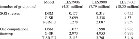
However, as shown in figure 10, the results from LES3900c (coarser resolution) with T-SR-FU are very similar to those from LES3900f (finer resolution) with DSM, indicating that one may reduce the number of grid points with T-SR-FU while keeping the same accuracy (note that the number of grid points of LES3900f is about twice that of LES3900c). The amount of CPU time for LES3900f with DSM is 2.986 seconds for advancing one computational timestep, but it is 2.113 seconds for LES3900c with T-SR-FU. This result suggests that the present NNs may not significantly increase overall CPU time by providing better accuracy with fewer grid points.


 Open access