





1. Introduction
Inspired by the efficiency of swimming animals such as dolphins (Kramer Reference Kramer1961; Babenko Reference Babenko2021) due to their flexible anisotropic skin, compliant surfaces have been extensively investigated for their potential to provide fluid dynamic benefits in aqueous flows, such as delaying laminar to turbulent transition and reducing turbulent drag (Riley et al. Reference Riley, Hak and Metcalfe1988; Gad-el Landahl Reference Landahl1962; Hak Reference Gad-el Hak2002). More recently, viscoelastic coatings over rigid walls were demonstrated to mitigate boundary-layer separation, shock oscillations and the skin friction coefficient in high-speed aerodynamics with air as the flowing medium (Pham, Gianikos & Narayanaswamy Reference Pham, Gianikos and Narayanaswamy2018; Walz & Narayanaswamy Reference Walz and Narayanaswamy2023; Chakravarty & Narayanaswamy Reference Chakravarty and Narayanaswamy2024).
Although the aforementioned studies were performed on stable viscoelastic surfaces, stability analysis of incompressible laminar flows over viscoelastic surfaces (Yeo Reference Yeo1988, Reference Yeo1990, Reference Yeo1992; Pfister, Fabbiane & Marquet Reference Pfister, Fabbiane and Marquet2022) revealed that the eigenspectrum of the coupled problem consists of two distinct families that resemble the individual flow and the solid eigenspectrum. An amplification of the modes of the former type gives rise to Tollmien–Schlichting instabilities that exist for laminar flows over rigid surfaces, albeit modified by the surface compliance. The latter gives rise to flow-induced structural instabilities over the viscoelastic surface that are, in turn, broadly classified into travelling wave flutter (TWF) and static divergence (SD) instabilities based on their amplification mechanism and structure. The TWF modes appear as low-amplitude, faster-moving convective instabilities travelling at material shear speeds in mildly damped viscoelastic coatings (Gad-el Hak Reference Gad-el Hak1986; Greidanus et al. Reference Greidanus, Delfos, Picken and Westerweel2022). In contrast, SD waves appear as slow-moving large-amplitude waves and typically occur over highly damped coatings (Gad-El-Hak, Blackwelder & Riley Reference Gad-El-Hak, Blackwelder and Riley1984; Carpenter & Garrad Reference Carpenter and Garrad1986).
The destabilisation of the viscoelastic coatings during the onset of TWF is driven by the irreversible energy transfer from the flow into the wall. Through stability calculations (Carpenter & Morris Reference Carpenter and Morris1990; Tsigklifis & Lucey Reference Tsigklifis and Lucey2017), it has been shown that viscoelastic surface deformations tend to modify the phase relationships between flow wall-normal velocity and pressure beneath the critical layer (wall-normal location where the local mean flow speed matches the viscoelastic surface wave speed), resulting in energy gain by the wall through pressure work. Recent numerical simulations showed that the pressure phase shift across the critical layer is driven by unsteady flow separation events which originate at wall deformation troughs (Esteghamatian, Katz & Zaki Reference Esteghamatian, Katz and Zaki2022). Moreover, both Rosti & Brandt (Reference Rosti and Brandt2017) and Esteghamatian et al. (Reference Esteghamatian, Katz and Zaki2022) showed that the large unstable deformations induce similar near-wall flow structures to rough walls. Experimental evidence (Zhang et al. Reference Zhang, Wang, Blake and Katz2017; Wang, Koley & Katz Reference Wang, Koley and Katz2020; Lu et al. Reference Lu, Xiang, Zaki and Katz2024) has shown that the deformation wave structure depends mainly on the viscoelastic coating properties rather than the flow itself. The linear stability analysis of Yeo, Zhao & Khoo (Reference Yeo, Zhao and Khoo2001) used a turbulent mean flow over viscoelastic surfaces and reproduced the surface wave characteristics observed in experiments (Gad-El-Hak et al. Reference Gad-El-Hak, Blackwelder and Riley1984; Carpenter & Garrad Reference Carpenter and Garrad1986). They also showed that the surface destabilisation mechanisms are similar for both laminar and turbulent flows, although the instabilities are triggered at much lower free-stream speeds in turbulent flows.
It is noteworthy that past research with flow/viscoelastic surface interactions were performed in aqueous media whose density matched the compliant materials. Therefore, the flow inertial forces were large enough to destabilise the viscoelastic surface even at very low speeds ( $O$
(1) ms−1). The non-dimensional wall compliance
$O$
(1) ms−1). The non-dimensional wall compliance $R = \rho _\infty U^2_\infty /E'$
, defined as the ratio of flow dynamic pressure to material Young’s modulus, where
$R = \rho _\infty U^2_\infty /E'$
, defined as the ratio of flow dynamic pressure to material Young’s modulus, where $\rho$
and
$\rho$
and $U$
are fluid density and velocity respectively. The wall compliance
$U$
are fluid density and velocity respectively. The wall compliance $R$
has been extensively used to delineate the boundaries of flow-induced surface instability onset; typically, the instabilities occur for
$R$
has been extensively used to delineate the boundaries of flow-induced surface instability onset; typically, the instabilities occur for $R\gt 1$
. For gaseous flows, the material density is significantly higher,
$R\gt 1$
. For gaseous flows, the material density is significantly higher, $O(10^3)$
, than that of the flow medium. As a result, for low subsonic speeds, the relative compliance is quite low for the surface to respond strongly to wall pressure fluctuations. This limitation can be potentially offset in high-speed flows where the inertial forces are large enough (
$O(10^3)$
, than that of the flow medium. As a result, for low subsonic speeds, the relative compliance is quite low for the surface to respond strongly to wall pressure fluctuations. This limitation can be potentially offset in high-speed flows where the inertial forces are large enough ( $R \sim \,1$
) owing to the high flow speeds to trigger observable flow/viscoelastic surface interactions, leading to surface instabilities; as such, no prior works have investigated TWF in supersonic flows.
$R \sim \,1$
) owing to the high flow speeds to trigger observable flow/viscoelastic surface interactions, leading to surface instabilities; as such, no prior works have investigated TWF in supersonic flows.
In this work, for the first time, TWF instabilities are experimentally demonstrated over isotropic viscoelastic surfaces placed beneath a supersonic turbulent boundary layer. Activating and controlling such instabilities can engender new interactions between the flow and solid surface which can create pathways for flow control. Elucidating the key physics that governs the outcome of the flow/surface interactions on the TWF characteristics and developing predictive capabilities of the wave features form other key contributions of this work. The central question that is explored is how parameters like high flow velocities, Mach number, variable density and coating thickness influence the instability onset and surface wave features. To answer this question, a comprehensive study of the impact of different driving parameters on the instability characteristics was made using linear stability analysis.
2. Methodology
2.1. Experimental set-up
Experiments were performed in a variable Mach number supersonic wind tunnel at North Carolina State University. Extensive details of the facility can be found in earlier publications made using this facility (Walz & Narayanaswamy Reference Walz and Narayanaswamy2023). This is a blow down wind tunnel whose test section measures 150 $\times$
150
$\times$
150 $\times$
650 mm. The tunnel test time was 10 s, which corresponded to stable free-stream pressure conditions (
$\times$
650 mm. The tunnel test time was 10 s, which corresponded to stable free-stream pressure conditions ( ${\lt} 3\,\%$
overall variation). The free-stream Mach numbers (
${\lt} 3\,\%$
overall variation). The free-stream Mach numbers ( $M_\infty$
) used in this study were primarily
$M_\infty$
) used in this study were primarily $M_\infty = 2.5$
with a few tests run at
$M_\infty = 2.5$
with a few tests run at $M_\infty = 3.0$
. The free-stream Mach number was determined to be within
$M_\infty = 3.0$
. The free-stream Mach number was determined to be within $ 0.02$
deviation between static to stagnation pressure ratios and Pitot to static pressure ratios. The stagnation pressure was varied between 380 and 930 kPa to span stable and unstable viscoelastic surfaces. Separate wall temperatures measurements were made before and after a 10 s test run. These were done using calibrated infrared cameras (Fluke Inc.). At the end of 10 s the wall temperature decreased to 295 K (note that the recovery temperature is 285 K). This causes an overall 1.6 percent uncertainty in the fluid density at the wall.
$ 0.02$
deviation between static to stagnation pressure ratios and Pitot to static pressure ratios. The stagnation pressure was varied between 380 and 930 kPa to span stable and unstable viscoelastic surfaces. Separate wall temperatures measurements were made before and after a 10 s test run. These were done using calibrated infrared cameras (Fluke Inc.). At the end of 10 s the wall temperature decreased to 295 K (note that the recovery temperature is 285 K). This causes an overall 1.6 percent uncertainty in the fluid density at the wall.
The uncertainty in the stagnation pressure is $1.4\,\text{kPa}$
, which is a combined effect of the proportional integral derivative controller that controls the valve opening to the stagnation chamber and sensor uncertainty. This results in 0.3 % uncertainty in determining
$1.4\,\text{kPa}$
, which is a combined effect of the proportional integral derivative controller that controls the valve opening to the stagnation chamber and sensor uncertainty. This results in 0.3 % uncertainty in determining $R$
for case A (lowest stagnation pressure setting) and 0.22 % uncertainty for case E (highest stagnation pressure setting) of table 2.
$R$
for case A (lowest stagnation pressure setting) and 0.22 % uncertainty for case E (highest stagnation pressure setting) of table 2.
The test article was an aluminium flat plate (381 $\times$
117 mm) that formed a part of the wind tunnel sidewall. A hollow cavity of 250
$\times$
117 mm) that formed a part of the wind tunnel sidewall. A hollow cavity of 250 $\times$
60 mm (
$\times$
60 mm ( $\approx$
20
$\approx$
20 $\delta$ $\times$
5
$\times$
5 $\delta$
) was scoured in the middle of the aluminium plate. Two bottom plates of dimensions (150 mm
$\delta$
) was scoured in the middle of the aluminium plate. Two bottom plates of dimensions (150 mm $\times$
60 mm) and (100
$\times$
60 mm) and (100 $\times$
60 mm) were fitted into the cavity. The plates were free to move in the wall-normal direction such that the cavity depth could be varied between 0 (rigid surface) and 12 mm. In this study, the downstream part (100 mm) was kept fixed at 0 mm to form a rigid surface. The upstream part (150 mm) was used to make non-zero cavity depths. The viscoelastic coating filled the cavity volume to generate a seamless transition of the flow over the viscoelastic surface. EcoFlex series 00-10 shore hardness rubber was used as the viscoelastic material. This was a two-part liquid pour rubber that naturally adhered to the aluminium base during the curing process. After the rubber was poured into the recess, the model was placed in a vacuum oven to go through multiple cycles of a degassing process before curing, to remove any trapped air bubbles within or on the implant surface. The storage modulus and loss tangent of the material were measured using a TA Instruments Dynamic Mechanical Analyzer (DMA 850). The zero frequency properties are
$\times$
60 mm) were fitted into the cavity. The plates were free to move in the wall-normal direction such that the cavity depth could be varied between 0 (rigid surface) and 12 mm. In this study, the downstream part (100 mm) was kept fixed at 0 mm to form a rigid surface. The upstream part (150 mm) was used to make non-zero cavity depths. The viscoelastic coating filled the cavity volume to generate a seamless transition of the flow over the viscoelastic surface. EcoFlex series 00-10 shore hardness rubber was used as the viscoelastic material. This was a two-part liquid pour rubber that naturally adhered to the aluminium base during the curing process. After the rubber was poured into the recess, the model was placed in a vacuum oven to go through multiple cycles of a degassing process before curing, to remove any trapped air bubbles within or on the implant surface. The storage modulus and loss tangent of the material were measured using a TA Instruments Dynamic Mechanical Analyzer (DMA 850). The zero frequency properties are $E'$
= 0.05 MPa,
$E'$
= 0.05 MPa, $E'' = 0.003$
MPa and the loss tangent
$E'' = 0.003$
MPa and the loss tangent $\phi = 0.06$
. The loss tangent is defined as
$\phi = 0.06$
. The loss tangent is defined as $\tan \phi = E''/E'$
. The frequency-dependent modulus values are shown in figure 1. It can be seen that both the storage and loss moduli increase with the forcing frequency. There is a sharp drop in both the storage and loss moduli at 1 Hz
$\tan \phi = E''/E'$
. The frequency-dependent modulus values are shown in figure 1. It can be seen that both the storage and loss moduli increase with the forcing frequency. There is a sharp drop in both the storage and loss moduli at 1 Hz $\lt f\lt$
2 Hz which is most likely a fixture or frame resonance artefact. Due to the frequency-dependent modulus values with data up to
$\lt f\lt$
2 Hz which is most likely a fixture or frame resonance artefact. Due to the frequency-dependent modulus values with data up to $30$
Hz, there is an ambiguity in the material constants that should be used in linear stability analysis, hence quantitative comparison between linear stability analysis and experiments is not performed.
$30$
Hz, there is an ambiguity in the material constants that should be used in linear stability analysis, hence quantitative comparison between linear stability analysis and experiments is not performed.
Storage ( $E'$
$E'$
 ) and loss ( $E''$
$E''$
 ) moduli as a function of frequency.

Figure 1. Long description
A two line graph showing storage and loss moduli as a function of frequency. The x-axis represents frequency in Hertz, ranging from 10^-2 to 10^2. The y-axis represents the moduli in megapascals, ranging from 10^-3 to 10^-1. The red line represents the storage modulus, which remains relatively constant around 10^-1 megapascals across the frequency range. The blue line represents the loss modulus, which starts around 10^-3 megapascals, increases to around 10^-2 megapascals, and then shows a significant dip before rising again. All values are approximated.
2.2. Measurement tools
Stereoscopic digital image correlation (Stereo-DIC) was performed to obtain two-dimensional surface displacement fields. For these campaigns, the translucent viscoelastic rubber was mixed with white silicone paint prior to curing, which made the surface opaque and enhanced the contrast for improved measurement quality. The surface speckle pattern was made by spraying with black India ink. The speckle pattern had good contrast, isotropy, features on average of approximately 5 pixels and covered a little more than 50 % of the surface. A spanwise centred 50 $\times$
50 mm region at the trailing edge of the viscoelastic implant formed the field of view (FOV). Two high-speed cameras (Photron Inc. Model: Nova S16) fitted with a Nikon 135 mm
$\times$
50 mm region at the trailing edge of the viscoelastic implant formed the field of view (FOV). Two high-speed cameras (Photron Inc. Model: Nova S16) fitted with a Nikon 135 mm $f/2D$
lens acquired the images. Extension rings (35 mm offset) were used to focus at small subject distances and the cameras were set at
$f/2D$
lens acquired the images. Extension rings (35 mm offset) were used to focus at small subject distances and the cameras were set at $20^\circ$
half-angle. The images were acquired at full resolution (1024
$20^\circ$
half-angle. The images were acquired at full resolution (1024 $\times$
1024 pixels), which provided an in-plane resolution of approximately 50 μm pixel−1. The acquired images were processed with the open source planar DIC tool Ncorr (Blaber, Adair & Antoniou Reference Blaber, Adair and Antoniou2015) and stereo reconstruction toolbox DuoDIC (Solav & Silverstein Reference Solav and Silverstein2022) to obtain the out-of-plane wall displacements. A subset size of 16 pixels was used, with a step size of 8 pixels to resolve fine-scale features. The speckle pattern was made to ensure that approximately 3–4 features were present within each subset.
$\times$
1024 pixels), which provided an in-plane resolution of approximately 50 μm pixel−1. The acquired images were processed with the open source planar DIC tool Ncorr (Blaber, Adair & Antoniou Reference Blaber, Adair and Antoniou2015) and stereo reconstruction toolbox DuoDIC (Solav & Silverstein Reference Solav and Silverstein2022) to obtain the out-of-plane wall displacements. A subset size of 16 pixels was used, with a step size of 8 pixels to resolve fine-scale features. The speckle pattern was made to ensure that approximately 3–4 features were present within each subset.
Complementary wall shear stress measurements were performed using direct shear CS-0310 wall shear stress sensors to provide more confidence to the boundary-layer fit. The data were acquired at 100 KHz and were low pass filtered at 40 KHz, which prevented any aliasing effect from higher-frequency nonlinear features in the sensor response as well as from the flow. The mean shear stress data were also within $\pm 5\,\%$
of oil film interferometry based mean shear measurements (not presented here for brevity). Moreover, the equilibrium fit parameters for the mean boundary-layer profile from both particle image velocimetry (PIV) and Pitot-based methods also report the wall shear stress to be within
$\pm 5\,\%$
of oil film interferometry based mean shear measurements (not presented here for brevity). Moreover, the equilibrium fit parameters for the mean boundary-layer profile from both particle image velocimetry (PIV) and Pitot-based methods also report the wall shear stress to be within $\pm 2\,\%$
of the measured value.
$\pm 2\,\%$
of the measured value.
Additionally, mean boundary-layer velocity measurements required for stability analysis were performed only over rigid metal surface by replacing the viscoelastic coating with a metal insert. The measurements were fit to a canonical turbulent boundary-layer profile using a least squares fit, as discussed in Appendix A. Figure 2 shows a schematic of the test article and locations of different measurements performed in this study. The boundary-layer profile measurements were performed within FOV of the stereo-DIC measurements, while wall shear stress measurements were performed 10 mm downstream of the FOV. During the mean velocity and wall shear measurements, the viscoelastic coating was removed and the recessed upstream plate was fixed at 0 mm to form a rigid wall.
Schematic of test article with locations for different measurements and speckle pattern for DIC.

Figure 2. Long description
The diagram illustrates a rectangular test article with dimensions of 15 centimeters by 6 centimeters. Within this rectangle, there is a smaller square area of 5 centimeters by 5 centimeters, which contains a 2 centimeters by 2 centimeters section. The diagram indicates the positions of a wall shear stress sensor and a pitot tube tip within this smaller square. Additionally, the right side of the image shows a speckle pattern used for DIC.
2.3. Linear stability analysis
We start with a compressible boundary layer with streamwise, wall-normal and spanwise directions as $x$
,
$x$
, $y$
and
$y$
and $z$
, or 1, 2 and 3, respectively. The compressible Navier–Stokes equations are compactly written in the form
$z$
, or 1, 2 and 3, respectively. The compressible Navier–Stokes equations are compactly written in the form
 \begin{equation} \frac {\partial {\boldsymbol{q}}_{\!f}}{\partial t} = N({\boldsymbol{q}}_{\!f}). \end{equation}
Here, $\boldsymbol{q}_{\!f} = [u_{\!f},v_{\!f},w_{\!f},\rho _{\!f},\theta ]^{\text{T}} \in {\mathbb{R}}^{5n_{\!f}}$
are the state variables of the fluid, and
$\boldsymbol{q}_{\!f} = [u_{\!f},v_{\!f},w_{\!f},\rho _{\!f},\theta ]^{\text{T}} \in {\mathbb{R}}^{5n_{\!f}}$
are the state variables of the fluid, and $n_{\!f}$
is the size of the discretised domain. The variables
$n_{\!f}$
is the size of the discretised domain. The variables $u_{\!f},v_{\!f},w_{\!f}$
represent the streamwise, wall-normal and spanwise velocities, respectively,
$u_{\!f},v_{\!f},w_{\!f}$
represent the streamwise, wall-normal and spanwise velocities, respectively, $\rho _{\!f}$
represents density and
$\rho _{\!f}$
represents density and $\theta$
represents temperature. All quantities are normalised by their free-stream values and length is normalised by the boundary-layer thickness
$\theta$
represents temperature. All quantities are normalised by their free-stream values and length is normalised by the boundary-layer thickness $\delta$
. The non-dimensional mean pressure is therefore constant and unity across the boundary layer. The non-dimensional equation of state therefore becomes
$\delta$
. The non-dimensional mean pressure is therefore constant and unity across the boundary layer. The non-dimensional equation of state therefore becomes
 \begin{align} p' = \bar {\theta }\rho ' + \bar {\rho }\theta ', \quad \bar {\rho }\bar {\theta } = 1. \end{align}
The Reynolds number is given by $Re_\delta = \rho _\infty U_\infty \delta /\mu _\infty$
, where
$Re_\delta = \rho _\infty U_\infty \delta /\mu _\infty$
, where $\delta$
is the boundary layer thickness. The wall is assumed to be at the adiabatic wall temperature. Using the parallel flow assumption, the state variables are decomposed into statistically stationary mean and fluctuating components, given by
$\delta$
is the boundary layer thickness. The wall is assumed to be at the adiabatic wall temperature. Using the parallel flow assumption, the state variables are decomposed into statistically stationary mean and fluctuating components, given by
 \begin{equation} \boldsymbol{q}_{\!f}(x,y,z,t) = \bar {\boldsymbol{q}}_{\!f}(y)+\boldsymbol{q}^{\prime }_{\!f}(x,y,z,t). \end{equation}
Here, $ \bar {\boldsymbol{q}}_{\!f}(y) = [\bar {u}_{\!f},0,0,\bar {\rho }_{\!f},\bar {\theta }_{\!f}]^T$
is the mean compressible turbulent boundary-layer profile. The fluctuations can be Fourier transformed in the homogeneous directions and written as
$ \bar {\boldsymbol{q}}_{\!f}(y) = [\bar {u}_{\!f},0,0,\bar {\rho }_{\!f},\bar {\theta }_{\!f}]^T$
is the mean compressible turbulent boundary-layer profile. The fluctuations can be Fourier transformed in the homogeneous directions and written as
 \begin{align} \boldsymbol{q}^{\prime }_{\!f}(x,y,z,t) = \int _{-\infty }^{\infty } \int _{-\infty }^{\infty } \int _{-\infty }^{\infty } \hat {\boldsymbol{q}}_{\!f}(y)e^{i(k_xx+k_zz-\omega t)} \text{d}k_x \text{d}k_z \text{d}\omega. \end{align}
Here, ( $k_x, k_z$
) are the wavenumbers in the streamwise and spanwise directions, and
$k_x, k_z$
) are the wavenumbers in the streamwise and spanwise directions, and $\omega$
is the circular frequency. Working with the Fourier transformed equations and ignoring the nonlinear terms, (2.1) can now be written in the eigenvalue form as
$\omega$
is the circular frequency. Working with the Fourier transformed equations and ignoring the nonlinear terms, (2.1) can now be written in the eigenvalue form as
 \begin{equation} I\omega \hat {\boldsymbol{q}}_{\!f} = A \hat {\boldsymbol{q}}_{\!f}, \end{equation}
Here, $A$
is the linearized Navier Stokes operator and
$A$
is the linearized Navier Stokes operator and $I$
is an identity matrix. According to the temporal stability ansatz, we allow the frequency to be complex (
$I$
is an identity matrix. According to the temporal stability ansatz, we allow the frequency to be complex ( $\omega = \omega _r+i\omega _i$
), such that
$\omega = \omega _r+i\omega _i$
), such that $\omega _i\gt 0$
denotes the onset of instability.
$\omega _i\gt 0$
denotes the onset of instability.
2.3.1. Compliant-wall effects
In order to describe the dynamics of the viscoelastic compliant coating, the following non-dimensional parameters are used:
 \begin{align} E = E^*/\rho _\infty U^2_\infty , \quad \mu _s = \mu ^*_s/\rho _\infty U_\infty \delta , \quad \rho _s = \rho ^*_s/\rho _\infty , \quad h = h^*/\delta. \end{align}
Here, $E^*$
is the Young’s modulus,
$E^*$
is the Young’s modulus, $\mu ^*_s$
is the solid viscosity,
$\mu ^*_s$
is the solid viscosity, $\rho ^*_s$
is the solid density and
$\rho ^*_s$
is the solid density and $h^*$
is the thickness of the coating. All solid parameters are also normalised by free-stream fluid quantities, and the boundary-layer thickness
$h^*$
is the thickness of the coating. All solid parameters are also normalised by free-stream fluid quantities, and the boundary-layer thickness $\delta$
is used as the length scale. All dimensional quantities are subsequently expressed using the asterisk
$\delta$
is used as the length scale. All dimensional quantities are subsequently expressed using the asterisk $^*$
. The dynamics of the incompressible solid is given by
$^*$
. The dynamics of the incompressible solid is given by
 \begin{equation} \rho _s \frac {\partial ^2\xi _i}{\partial t^2}= \frac {\partial \sigma ^s_{\textit{ij}}}{\partial x_{\!j}}, \quad \frac {\partial \xi _i}{\partial x_i} = 0. \end{equation}
Here, $\boldsymbol{s} = [\xi _1, \xi _2, \xi _3]^T \in \mathbb{R}^{3n_s}$
is the infinitesimal solid displacement, and
$\boldsymbol{s} = [\xi _1, \xi _2, \xi _3]^T \in \mathbb{R}^{3n_s}$
is the infinitesimal solid displacement, and $\sigma ^s_{\textit{ij}}$
is the infinitesimal solid stress tensor. Using the Kelvin–Voigt viscoelastic model, the stress tensor
$\sigma ^s_{\textit{ij}}$
is the infinitesimal solid stress tensor. Using the Kelvin–Voigt viscoelastic model, the stress tensor $\sigma ^s_{\textit{ij}}$
is given by
$\sigma ^s_{\textit{ij}}$
is given by
 \begin{align} \sigma ^s_{\textit{ij}} = -p_s\delta _{\textit{ij}} + G\big (\epsilon _{\textit{ij}} + \epsilon _{\textit{ji}}\big) + \mu _s\big (\dot {\epsilon }_{\textit{ij}} + \dot {\epsilon }_{\textit{ji}}\big). \end{align}
Here, $p_s$
is the solid pressure which is used to satisfy the incompressibility constraint,
$p_s$
is the solid pressure which is used to satisfy the incompressibility constraint, $G = E/3$
is the material shear modulus,
$G = E/3$
is the material shear modulus, $\epsilon _{\textit{ij}}$
is the strain and
$\epsilon _{\textit{ij}}$
is the strain and $\dot {\epsilon }_{\textit{ij}}$
is the strain rate. Both
$\dot {\epsilon }_{\textit{ij}}$
is the strain rate. Both $p_s$
and
$p_s$
and $G$
are normalised using the free-stream dynamic pressure. Since we are looking at modes of the type
$G$
are normalised using the free-stream dynamic pressure. Since we are looking at modes of the type $\hat {\phi }(y)e^{i(k_x x + k_z z - \omega t)}$
, (2.8) can be re-written using the complex shear modulus
$\hat {\phi }(y)e^{i(k_x x + k_z z - \omega t)}$
, (2.8) can be re-written using the complex shear modulus
 \begin{align} \sigma ^s_{\textit{ij}} = -p_s\delta _{\textit{ij}} + (G - i\omega \mu _s)\left (\epsilon _{\textit{ij}}+ \epsilon _{\textit{ji}}\right )\! . \end{align}
The viscoelastic coating extended from $y=0$
to
$y=0$
to $y = -h$
in the wall-normal direction, and infinitely in the other two directions. The coating was free to deform at the top (
$y = -h$
in the wall-normal direction, and infinitely in the other two directions. The coating was free to deform at the top ( $y=0$
) but clamped at the bottom
$y=0$
) but clamped at the bottom $\xi (-h) = 0$
. It must be noted that we have ignored the mean deformation terms that are present when using the neo-Hookean model due its sub-micron values observed in the experiments. To couple the governing fluid and solid equations, velocity and stress continuity is satisfied at the interface. The modified no-slip conditions at the interface
$\xi (-h) = 0$
. It must be noted that we have ignored the mean deformation terms that are present when using the neo-Hookean model due its sub-micron values observed in the experiments. To couple the governing fluid and solid equations, velocity and stress continuity is satisfied at the interface. The modified no-slip conditions at the interface $(y = 0)$
are given by
$(y = 0)$
are given by
 \begin{align} \begin{split} -i\omega \hat {\xi }_1 = \hat {u}_{\!f}+\hat {\xi }_2 \frac {\partial \bar {u}_{\!f}}{\partial y}, \quad -i\omega \hat {\xi }_2 = \hat {v}_{\!f}, \quad -i\omega \hat {\xi }_3 = \hat {w}_{\!f}. \end{split} \end{align}
The continuity of stresses at $y=0$
for a two-dimensional case is given as
$y=0$
for a two-dimensional case is given as
 \begin{align} \begin{split} &\hat {\sigma }^s_{12}: ({G} - i\omega \mu _s)\left (\frac {\partial \hat {\xi }_1}{\partial x_2}+\frac {\partial \hat {\xi }_2}{\partial x_1}\right ) = {\hat {\sigma }^f_{12}}, \\[3pt] &\hat {\sigma }^f_{12} = \frac {1}{Re_\delta }\left [\bar {\mu }_{\!f}\left (\frac {\partial \hat {u}^f_1}{\partial x_2}+\frac {\partial \hat {u}^f_2}{\partial x_1}+{\hat {\xi _2}\frac {\partial ^2\bar {u}^f_1}{\partial x_2^2}}\right ) + \frac {\text{d}\bar {\mu }_{\!f}}{\text{d}\theta }\frac {\text{d}\bar {u}^f_1}{dy}\hat {\theta }\right ]\!, \\[3pt] &\hat {\sigma }^s_{22}: -\hat {p}_s + 2(G - i\omega {\mu }_s)\frac {\partial \hat {\xi }_2}{\partial x_2} = \hat {\sigma }^f_{22}, \\[3pt] &\hat {\sigma }^f_{22} = -\frac {1}{\gamma M^2_\infty }\hat {p}_{\!f} + \frac {1}{Re_\delta }\left [ 2\bar {\mu }_{\!f}\frac {\partial \hat {u}^f_2}{\partial x_2} + \bar {\lambda }\left ( \frac {\partial \hat {u}^f_1}{\partial x_1} + \frac {\partial \hat {u}^f_2}{\partial x_2}\right ) \right ]\!. \end{split} \end{align}
Sutherland’s law was used to relate the mean fluid viscosity $\bar {\mu }_{\!f}$
to the mean temperature.
$\bar {\mu }_{\!f}$
to the mean temperature.
In the free stream, the velocity and temperature perturbations are set to zero. The temperature perturbations at the solid surface are also set to zero. For state variables with homogeneous boundary conditions, the corresponding rows and columns are removed to avoid singular matrices. Since the interface expressions (2.10, 2.11) contain the eigenvalue $\omega$
, the corresponding rows are simply replaced by the interface equations. After assembling (2.5–2.11), the resulting fluid-structural operator can be written as a quadratic eigenvalue problem
$\omega$
, the corresponding rows are simply replaced by the interface equations. After assembling (2.5–2.11), the resulting fluid-structural operator can be written as a quadratic eigenvalue problem
 \begin{equation} \big (K+D\omega + M\omega ^2\big ) \left (\begin{array}{c} \hat {\boldsymbol{q}}_{\!f} \\[5pt] \hat {\boldsymbol{q}}_s \end{array}\right )= 0. \end{equation}
Here, $\hat {\boldsymbol{q}}_s = [\hat {\xi }_1, \hat {\xi }_2, \hat {\xi }_3]^T$
are the state variables of the solid. Using the companion matrix method, this can be recast into a generalised eigenvalue problem given by
$\hat {\boldsymbol{q}}_s = [\hat {\xi }_1, \hat {\xi }_2, \hat {\xi }_3]^T$
are the state variables of the solid. Using the companion matrix method, this can be recast into a generalised eigenvalue problem given by
 \begin{align} (A + B\omega )\left (\begin{array}{c} \hat {\boldsymbol{q}}_{\!f} \\[5pt] \hat {\boldsymbol{q}}_s \\[5pt] \omega \hat {\boldsymbol{q}}_s \\ \end{array}\right )= 0. \end{align}
The matrices $A$
and
$A$
and $B$
are of the form
$B$
are of the form
 \begin{align} A = \begin{bmatrix} K & 0\\[3pt] 0 & I \end{bmatrix}, \quad B = \begin{bmatrix} D & M\\[3pt] -I & 0 \end{bmatrix}\!. \end{align}
The fluid domain was discretised into $n_{\!f} =$
401 points in the wall-normal
$n_{\!f} =$
401 points in the wall-normal $(y)$
direction using Chebyshev collocation points. A grid transformation was used to maintain near-wall resolution, given by
$(y)$
direction using Chebyshev collocation points. A grid transformation was used to maintain near-wall resolution, given by $y = ay_c/(b-y_c)$
(Schmid, Henningson & Jankowski Reference Schmid, Henningson and Jankowski2002), where
$y = ay_c/(b-y_c)$
(Schmid, Henningson & Jankowski Reference Schmid, Henningson and Jankowski2002), where $-1\leqslant y_c \leqslant 1$
represents the Chebyshev points, and the domain size was kept at
$-1\leqslant y_c \leqslant 1$
represents the Chebyshev points, and the domain size was kept at $5 \delta$
. For the compliant wall,
$5 \delta$
. For the compliant wall, $n_s =$
51 Chebyshev points were used to discretise the wall from
$n_s =$
51 Chebyshev points were used to discretise the wall from $y = 0$
to
$y = 0$
to $y = -h$
.
$y = -h$
.
Flow parameters for case B.

Table 1. Long description
The table presents flow parameters for case B, detailing six variables across one case. The variables include free stream velocity in meters per second, boundary layer thickness in millimeters, air density in kilograms per cubic meter, friction velocity in meters per second, skin friction coefficient, and Reynolds number. The table has one row and six columns. Row 1: Case B, U infinity 588 meters per second, delta sub 99 12 millimeters, rho infinity 0.72 kilograms per cubic meter, u tau 21.2 meters per second, C sub f 0.0012, Re tau 4650.
Details of all experimental cases.

Table 2. Long description
The table presents a comparison of various experimental cases, detailing parameters such as height in millimeters, wall compliance, density ratios, Mach number, and diameter in millimeters. The table consists of six rows and seven columns. The columns are labeled as Case, h* (mm), R, rho_infinity/rho_s*, rho_w/rho_s*, M_infinity, and d_y (mm). Each row provides specific values for these parameters across different cases labeled A through F. Notable trends include variations in density ratios and Mach numbers across the cases, with specific values for each parameter provided for detailed analysis.
Since a turbulent mean flow is considered, the perturbation Reynolds stresses need to be included in the flow equations. This is done by using the Boussinesq hypothesis, and the Johnson–King eddy viscosity model (Johnson & King Reference Johnson and King1985) is used. The turbulent viscosity $\mu _t$
is given by
$\mu _t$
is given by
 \begin{align} \begin{split} &\mu _t=\kappa {\mu } y^* D\!\left (M_\tau \right )\!, \\[5pt] &D\!\left (M_\tau \right )=\left [1-\exp \left (\frac {-y^*}{A^{+}+f\left (M_\tau \right )}\right )\right ]^2 \!, \\[5pt] & A^{+}=17, \kappa =0.41, \text{ and } f\!\left (M_\tau \right )=19.3 M_\tau. \end{split} \end{align}
Here, $M_\tau =u_{\tau , w} / a_w$
, where
$M_\tau =u_{\tau , w} / a_w$
, where $a_w$
is the speed of sound at the wall. The semi-local coordinate
$a_w$
is the speed of sound at the wall. The semi-local coordinate $y^*$
is given by
$y^*$
is given by $y^* = y Re_\tau \sqrt {\bar {\rho }/\bar {\rho }_w}\bar {\mu }_w/\bar {\mu }$
. The Reynolds stress perturbations are given by
$y^* = y Re_\tau \sqrt {\bar {\rho }/\bar {\rho }_w}\bar {\mu }_w/\bar {\mu }$
. The Reynolds stress perturbations are given by
 \begin{align} -\bar {\rho }\overline {u'_1 u'_2} = \bar {\mu }_t\left (\frac {\partial u'_1}{\partial x_2} + \frac {\partial u'_2}{\partial x_1}\right ) + \mu '_t \frac {\partial \bar {U}}{\partial x_2}. \end{align}
Equation (2.16) is added to the $x$
and
$x$
and $y$
momentum equations along with the other viscous terms. The turbulent viscosity perturbations are given by
$y$
momentum equations along with the other viscous terms. The turbulent viscosity perturbations are given by $\mu '_t = ({\text{d}\bar {\mu }_t}/{\text{d}\bar {\theta }})\theta '$
, and they occur due to the dependence of
$\mu '_t = ({\text{d}\bar {\mu }_t}/{\text{d}\bar {\theta }})\theta '$
, and they occur due to the dependence of $\mu _t$
on
$\mu _t$
on $\mu$
. It must be noted that, since
$\mu$
. It must be noted that, since $\mu _t$
and
$\mu _t$
and $\mu '_t$
are zero at
$\mu '_t$
are zero at $y=0$
, the Reynolds stress terms do not directly force the viscoelastic surface at the first order.
$y=0$
, the Reynolds stress terms do not directly force the viscoelastic surface at the first order.
Supersonic boundary-layer mean profiles were generated for every flow configuration studied. The detailed method is discussed in Appendix A.
3. Results
3.1. Experiments
Overall, five sets of wind tunnel runs were conducted, capturing variations in the Reynolds and Mach numbers, as well as different viscoelastic coating thicknesses. Salient details from each run are shown in table 2, and flow parameters from case B are shown in table 1. Here, $d_y$
represents the root mean square deformation magnitudes and
$d_y$
represents the root mean square deformation magnitudes and $h \text{(mm)}$
denotes the viscoelastic coating thickness. For cases
$h \text{(mm)}$
denotes the viscoelastic coating thickness. For cases $\textrm{A}{-}\textrm{C}$
, the Mach number and coating thickness were held constant, and the stagnation pressure of the wind tunnel was increased gradually. This increased the free-stream static pressure and therefore the free-stream dynamic pressure (note
$\textrm{A}{-}\textrm{C}$
, the Mach number and coating thickness were held constant, and the stagnation pressure of the wind tunnel was increased gradually. This increased the free-stream static pressure and therefore the free-stream dynamic pressure (note $q_\infty = 1/2 \rho _\infty u_\infty ^2 = 1/2 \gamma p_\infty M_\infty ^2$
), which increased the wall compliance
$q_\infty = 1/2 \rho _\infty u_\infty ^2 = 1/2 \gamma p_\infty M_\infty ^2$
), which increased the wall compliance $R$
, as shown in table 2. For case
$R$
, as shown in table 2. For case $D$
, the Mach number was increased to
$D$
, the Mach number was increased to $M_\infty = 3$
, while the free-stream density and Reynolds number were kept similar to case
$M_\infty = 3$
, while the free-stream density and Reynolds number were kept similar to case $B$
. Between cases
$B$
. Between cases $\textrm{B}$
and
$\textrm{B}$
and $D$
, only
$D$
, only $M_\infty$
and wall compliance
$M_\infty$
and wall compliance $R$
were varied. This served the purpose of studying how the critical compliance for onset of instability
$R$
were varied. This served the purpose of studying how the critical compliance for onset of instability $R_{\textit{onset}}$
may change due to variations in
$R_{\textit{onset}}$
may change due to variations in $M_\infty$
. For case
$M_\infty$
. For case $E$
, the Mach number was maintained at
$E$
, the Mach number was maintained at $M_\infty = 2.5$
and the coating thickness was decreased to
$M_\infty = 2.5$
and the coating thickness was decreased to $1.8$
mm. Using case
$1.8$
mm. Using case $E$
, we aim to study how instability wave characteristics and
$E$
, we aim to study how instability wave characteristics and $R_{\textit{onset}}$
may change with coating thickness.
$R_{\textit{onset}}$
may change with coating thickness.
During a given test run, the stagnation temperature and pressure and static pressure at the wall provide the measurements of $\rho _\infty$
and
$\rho _\infty$
and $U_\infty$
, which were used to get the compliance values. The onset of surface instability was determined by analysing the surface deformation fields visually and using power spectra to detect coherent wave structures on the surface. The wind tunnel stagnation pressure decreased by
$U_\infty$
, which were used to get the compliance values. The onset of surface instability was determined by analysing the surface deformation fields visually and using power spectra to detect coherent wave structures on the surface. The wind tunnel stagnation pressure decreased by $2\,\%{-} 3\,\%$
over the course of a test run. This gives approximately 2 %–3 % uncertainty in the values of
$2\,\%{-} 3\,\%$
over the course of a test run. This gives approximately 2 %–3 % uncertainty in the values of $R$
, which is much smaller than the range of variations explored in table 2.
$R$
, which is much smaller than the range of variations explored in table 2.
3.1.1. Critical parameters of instability onset
Figure 3(a–c) shows a series of instantaneous wall-normal deformation fields of the viscoelastic surface at different wall compliance ( $R$
) ratios to portray the onset of surface instability for a
$R$
) ratios to portray the onset of surface instability for a $M_\infty = 2.5$
flow, where
$M_\infty = 2.5$
flow, where $M_\infty$
is the free-stream Mach number. The free-stream dynamic pressure (and compliance
$M_\infty$
is the free-stream Mach number. The free-stream dynamic pressure (and compliance $R$
) at a given Mach number was increased by only increasing the free-stream pressure while the free-stream Mach number remained constant. Figure 3(a) (case A) shows the absence of any coherent wavelike undulations on the surface for the lowest
$R$
) at a given Mach number was increased by only increasing the free-stream pressure while the free-stream Mach number remained constant. Figure 3(a) (case A) shows the absence of any coherent wavelike undulations on the surface for the lowest $R$
, which evidences a stable surface at this dynamic pressure. As the dynamic pressure (and
$R$
, which evidences a stable surface at this dynamic pressure. As the dynamic pressure (and $R$
) was increased, spanwise coherent patches of undulations occur on the surface, as shown in figure 3(b) (case B). Increasing the flow dynamic pressure further causes the undulations to become fully spanwise coherent along with an increase in the deformation magnitude (figure 3(c), case C), and the surface is completely destabilised at this flow configuration.
$R$
) was increased, spanwise coherent patches of undulations occur on the surface, as shown in figure 3(b) (case B). Increasing the flow dynamic pressure further causes the undulations to become fully spanwise coherent along with an increase in the deformation magnitude (figure 3(c), case C), and the surface is completely destabilised at this flow configuration.
Transition from stable to unstable response at $M_\infty = 2.5$
by increasing stagnation pressure; (a)
$M_\infty = 2.5$
by increasing stagnation pressure; (a) $R = 4.5$
, (b)
$R = 4.5$
, (b) $R = 5.3$
, (c)
$R = 5.3$
, (c) $R = 6$
and (d)
$R = 6$
and (d) $R = 6$
,
$R = 6$
, $M_\infty = 3$
. The thickness of the viscoelastic implant was 5 mm for all cases.
$M_\infty = 3$
. The thickness of the viscoelastic implant was 5 mm for all cases.

Figure 3. Long description
A heat map showing the transition from stable to unstable response by increasing stagnation pressure. The heat map consists of four subplots labeled (a), (b), (c), and (d). Each subplot represents different conditions of the response. The x-axis is labeled ‘X (mm)’ and ranges from 100 to 150 millimeters, while the y-axis is labeled ‘Z (mm)’ and ranges from -20 to 20 millimeters. The color scale at the top of each subplot indicates the displacement in the y-direction (d_y) in millimeters, with blue representing negative values and red representing positive values. Subplot (a) has a color scale ranging from -0.02 to 0.02 millimeters, subplot (b) ranges from -0.06 to 0.06 millimeters, subplot (c) ranges from -0.4 to 0.2 millimeters, and subplot (d) ranges from -0.03 to 0.03 millimeters. The heat maps show varying patterns of displacement, with subplot (a) displaying a more scattered distribution, subplot (b) showing more defined streaks, subplot (c) exhibiting prominent wave-like patterns, and subplot (d) presenting a mix of scattered and streaked patterns. The thickness of the viscoelastic implant was 5 millimeters for all cases.
Now, while keeping the viscoelastic coating parameters fixed, the free-stream Mach number, $M_\infty$
, was increased to 3.0. The flow parameters for all the cases in figure 3 are listed in table 2. Figure 3(d) shows an instantaneous image of surface deformation at
$M_\infty$
, was increased to 3.0. The flow parameters for all the cases in figure 3 are listed in table 2. Figure 3(d) shows an instantaneous image of surface deformation at $R = 6$
, (case D). Comparing figures 3(d) and 3(b), it is seen that the surface is stable at
$R = 6$
, (case D). Comparing figures 3(d) and 3(b), it is seen that the surface is stable at $R = 6$
at Mach 3 while it was already unstable at a lower wall compliance
$R = 6$
at Mach 3 while it was already unstable at a lower wall compliance $R = 5.3$
at Mach 2.5. In fact, instabilities are triggered at
$R = 5.3$
at Mach 2.5. In fact, instabilities are triggered at $R \approx 6.2$
at
$R \approx 6.2$
at $M_\infty = 3$
, which is substantially higher than the onset limit of
$M_\infty = 3$
, which is substantially higher than the onset limit of $R \approx 5$
at
$R \approx 5$
at $M_\infty = 2.5$
. The free-stream speed increased by 7 % from
$M_\infty = 2.5$
. The free-stream speed increased by 7 % from $M_\infty = 2.5$
to
$M_\infty = 2.5$
to $M_\infty = 3$
. Comparing between case B (figure 3
b) and case D (figure 3
d), the free-stream densities are found to be similar, while the flow density at the wall is lower by 19 % for case D at
$M_\infty = 3$
. Comparing between case B (figure 3
b) and case D (figure 3
d), the free-stream densities are found to be similar, while the flow density at the wall is lower by 19 % for case D at $M_\infty = 3$
.
$M_\infty = 3$
.
The above discussion provides two major pointers on the flow parameters that govern the onset of instability. First, there was only a minor change in the free-stream speed between the two different Mach numbers that exhibited a substantial change in the $R_{\textit{onset}}$
. Therefore, the free-stream velocity and dynamic pressure are not the singular parameters that govern the onset, as was the case for incompressible flows. Secondly, the flow parameters corresponding to figures 3(a), 3(b) and 3(d) suggest the free-stream Mach number
$R_{\textit{onset}}$
. Therefore, the free-stream velocity and dynamic pressure are not the singular parameters that govern the onset, as was the case for incompressible flows. Secondly, the flow parameters corresponding to figures 3(a), 3(b) and 3(d) suggest the free-stream Mach number $M_\infty$
also plays an important role in destabilising the viscoelastic surface at high speeds.
$M_\infty$
also plays an important role in destabilising the viscoelastic surface at high speeds.
3.2. Linear stability analysis
Local stability analysis was used to understand the parametric trends and wave characteristics observed in the experiments, as well as to shed light on the driving mechanisms of these instabilities. Using the temporal stability ansatz in (2.4), an unstable eigenmode is identified by a positive imaginary part of its associated eigenvalue. The stability margins and wave characteristics of the principal modes of the combined fluid–structure system with respect to key non-dimensional parameters of the flow and solid are presented.
The effect of wall parameters on the least stable fluid-elastic mode is first studied. The reference case for the parametric study closely corresponds to case C in table 2, with the parameters $E^*/\rho _\infty U^2_\infty = 1/R = 0.6, h^*/\delta = 0.5, \rho ^*_s/\rho _\infty = 1000,{} \mu ^*_s/\rho _\infty U_\infty \delta = 0.8, M_\infty = 2.5 \text{ and } Re_\tau = 5000$
. For the stability calculations, a higher range of Young’s modulus is used, which corresponds to its measured values at higher frequencies (
$E^*/\rho _\infty U^2_\infty = 1/R = 0.6, h^*/\delta = 0.5, \rho ^*_s/\rho _\infty = 1000,{} \mu ^*_s/\rho _\infty U_\infty \delta = 0.8, M_\infty = 2.5 \text{ and } Re_\tau = 5000$
. For the stability calculations, a higher range of Young’s modulus is used, which corresponds to its measured values at higher frequencies ( $E^* = 0.2$
MPa; figure 1). This is due to the fact that the frequencies of the dominant travelling waves were measured to be in the range 900–2500 Hz across all cases. With increasing frequency, the measured value is expected to increase further and plateau. In all the cases studied subsequently, the non-dimensional coating viscosity was fixed at
$E^* = 0.2$
MPa; figure 1). This is due to the fact that the frequencies of the dominant travelling waves were measured to be in the range 900–2500 Hz across all cases. With increasing frequency, the measured value is expected to increase further and plateau. In all the cases studied subsequently, the non-dimensional coating viscosity was fixed at $\mu ^*_s = 5.5$
. In figure 4, the non-dimensional temporal growth rates are shown against the streamwise wavenumber (
$\mu ^*_s = 5.5$
. In figure 4, the non-dimensional temporal growth rates are shown against the streamwise wavenumber ( $k_x$
) for different individual parametric studies. The temporal growth rates are non-dimensionalised by the flow variables, whereas the wavenumber is non-dimensionalised by the viscoelastic coating thickness (
$k_x$
) for different individual parametric studies. The temporal growth rates are non-dimensionalised by the flow variables, whereas the wavenumber is non-dimensionalised by the viscoelastic coating thickness ( $h$
). The growth rates for the reference case is shown in red. Figure 4 (a–c) corresponds to variations only in the parameters of the solid, whereas figure 4(d) corresponds to variations in the Mach number.
$h$
). The growth rates for the reference case is shown in red. Figure 4 (a–c) corresponds to variations only in the parameters of the solid, whereas figure 4(d) corresponds to variations in the Mach number.
Parametric variation of instability growth rate across: (a) material Young’s modulus, (b) coating thickness, (c) material density, (d) Mach number.

Figure 4. Long description
The image contains four line graphs labeled (a) through (d), each depicting the parametric variation of instability growth rate across different variables. Graph (a) shows the variation with material Young’s modulus, with two lines representing different values of E divided by rho infinity U infinity squared. Graph (b) illustrates the variation with coating thickness, with two lines for different values of h. Graph (c) presents the variation with material density, with two lines for different values of rho s divided by rho infinity. Graph (d) shows the variation with Mach number, with two lines for different values of M infinity. Each graph has the x-axis labeled as kxh and the y-axis labeled as omega i. The lines in each graph represent different conditions or parameters, showing how the instability growth rate changes with the respective variable.
The effect of the viscoelastic material elastic modulus ( $E$
) is studied in figure 4(a). The reference case consists of unstable wavenumbers that range from
$E$
) is studied in figure 4(a). The reference case consists of unstable wavenumbers that range from $k_xh = 1 \text{ to } k_xh = 3.5$
. It can be seen that increasing the modulus of elasticity results in a notable decrease in the growth rates across all the wavenumbers. This is because the increase in
$k_xh = 1 \text{ to } k_xh = 3.5$
. It can be seen that increasing the modulus of elasticity results in a notable decrease in the growth rates across all the wavenumbers. This is because the increase in $E$
results in smaller deformations and an increase in the characteristic shear wave speed of the coating (
$E$
results in smaller deformations and an increase in the characteristic shear wave speed of the coating ( $C_t = \sqrt {E/3\rho _s}$
); the latter in turn elevates the critical layer away from the surface, and mitigates the energy transfer from fluid to solid. Decrease in deformations and elevation in critical layer height both delay the onset of instability. For both the cases studied, the maximum growth rate occurs at a streamwise wavenumber,
$C_t = \sqrt {E/3\rho _s}$
); the latter in turn elevates the critical layer away from the surface, and mitigates the energy transfer from fluid to solid. Decrease in deformations and elevation in critical layer height both delay the onset of instability. For both the cases studied, the maximum growth rate occurs at a streamwise wavenumber, $k_x h \approx 2$
, which closely corresponds to
$k_x h \approx 2$
, which closely corresponds to $\lambda = 3h$
.
$\lambda = 3h$
.
Next, the effect of viscoelastic coating thickness is studied in figure 4(b) that compares the coating thickness of $h = 0.4$
with the reference
$h = 0.4$
with the reference $h = 0.5$
. The decrease in coating thickness results in a strong reduction in temporal growth rates; all wavenumbers for
$h = 0.5$
. The decrease in coating thickness results in a strong reduction in temporal growth rates; all wavenumbers for $h = 0.4$
thickness are found to be stable. This effect is discussed in more detail later. Finally, the effect of viscoelastic material density
$h = 0.4$
thickness are found to be stable. This effect is discussed in more detail later. Finally, the effect of viscoelastic material density $\rho _s$
is studied. The growth rates are shown in figure 4(c) by comparing
$\rho _s$
is studied. The growth rates are shown in figure 4(c) by comparing $\rho _s = 1500$
with a reference
$\rho _s = 1500$
with a reference $\rho _s = 1000$
. Note that this parametric case does not have a clear experimental equivalent, since only a single viscoelastic material was used in the experimental study. Moreover, in the wind tunnel experiments the free-stream density cannot be individually varied while keeping all other non-dimensional parameters constant. Figure 4(c) shows that increasing
$\rho _s = 1000$
. Note that this parametric case does not have a clear experimental equivalent, since only a single viscoelastic material was used in the experimental study. Moreover, in the wind tunnel experiments the free-stream density cannot be individually varied while keeping all other non-dimensional parameters constant. Figure 4(c) shows that increasing $\rho _s$
results in slightly larger amplification rates. However, the change in growth rates is not as strong as was observed in figures 4(a) and 4(b). The observed increase in growth rates is counterintuitive, since it is known that, when one-way coupling is present, increasing
$\rho _s$
results in slightly larger amplification rates. However, the change in growth rates is not as strong as was observed in figures 4(a) and 4(b). The observed increase in growth rates is counterintuitive, since it is known that, when one-way coupling is present, increasing $\rho _s$
results in smaller deformations (Benschop et al. Reference Benschop, Greidanus, Delfos, Westerweel and Breugem2019). In this case, however, since
$\rho _s$
results in smaller deformations (Benschop et al. Reference Benschop, Greidanus, Delfos, Westerweel and Breugem2019). In this case, however, since $C_t = \sqrt {E/3\rho _s}$
, increasing the viscoelastic material density decreases the shear wave speed, which may result in the critical layer moving closer to the surface, resulting in larger energy transfer and amplification rates (Tsigklifis & Lucey Reference Tsigklifis and Lucey2017). The effect of the free-stream Mach number
$C_t = \sqrt {E/3\rho _s}$
, increasing the viscoelastic material density decreases the shear wave speed, which may result in the critical layer moving closer to the surface, resulting in larger energy transfer and amplification rates (Tsigklifis & Lucey Reference Tsigklifis and Lucey2017). The effect of the free-stream Mach number $M_\infty$
is considered next, which corresponds to case D from table 2; the compliance parameter
$M_\infty$
is considered next, which corresponds to case D from table 2; the compliance parameter $R$
in case C is repeated in case D. Figure 4(d) shows the variation in growth rates with the free-stream Mach number, while the non-dimensional structural parameters remained fixed. It is seen that increasing the Mach number results in reduced amplification. In all of the above cases, it is consistently observed that peak amplification occurs for waves with
$R$
in case C is repeated in case D. Figure 4(d) shows the variation in growth rates with the free-stream Mach number, while the non-dimensional structural parameters remained fixed. It is seen that increasing the Mach number results in reduced amplification. In all of the above cases, it is consistently observed that peak amplification occurs for waves with $ 1.5/h \lt k_x\lt 3/h$
.
$ 1.5/h \lt k_x\lt 3/h$
.
(a) Leading singular value from SPOD across different frequencies, (b) SPOD mode shapes corresponding to distinctive peaks.

Figure 5. Long description
The image contains two graphs: a line graph and four heat maps. The line graph on the left shows the leading singular value from SPOD across different frequencies for two different heights, represented by red and blue lines. The x-axis is labeled with the dimensionless frequency, and the y-axis is labeled with the singular value in square millimeters per Hertz. The red line represents a height of 1.8 millimeters, and the blue line represents a height of 5 millimeters. The graph highlights four distinctive peaks labeled A, B, C, and D. The four heat maps on the right show the SPOD mode shapes corresponding to these peaks. Each heat map is labeled with the corresponding peak letter and displays the spatial distribution of the mode shapes in the X-Z plane. The heat maps use a color gradient to represent the amplitude of the modes, with red indicating higher amplitudes and blue indicating lower amplitudes. The heat maps provide a visual representation of the spatial structure of the instabilities at different frequencies.
4. Discussion
4.1. Energetic modes of surface waves
To examine the validity of the above results in terms of the wave features, surface wall-normal deformation fields of the TWF over viscoelastic coatings were obtained at two different coating thicknesses ( $5$
mm or
$5$
mm or $h = 0.4$
and
$h = 0.4$
and $1.8$
mm or
$1.8$
mm or $h = 0.15$
), which correspond to cases
$h = 0.15$
), which correspond to cases $\textrm{C}$
and
$\textrm{C}$
and $E$
in table 2. Spectral proper orthogonal decomposition (SPOD) was used to extract the dominant advective features on the viscoelastic surface. Figure 5(a) shows the leading singular value across frequencies for implants of different thicknesses. The frequency is non-dimensionalised by the characteristic coating frequency based on the shear speed
$E$
in table 2. Spectral proper orthogonal decomposition (SPOD) was used to extract the dominant advective features on the viscoelastic surface. Figure 5(a) shows the leading singular value across frequencies for implants of different thicknesses. The frequency is non-dimensionalised by the characteristic coating frequency based on the shear speed $C_t$
and thickness
$C_t$
and thickness $h$
. The dominant features in both cases are marked
$h$
. The dominant features in both cases are marked $A{-}D$
. The
$A{-}D$
. The $5$
mm implant exhibits significantly stronger peaks compared with the
$5$
mm implant exhibits significantly stronger peaks compared with the $1.8$
mm implant, exhibiting higher energy overall. The dominant modes in both implants collapse well with the non-dimensional frequency. The mode shapes corresponding to these peaks are shown in figure 5(b). The feature marked
$1.8$
mm implant, exhibiting higher energy overall. The dominant modes in both implants collapse well with the non-dimensional frequency. The mode shapes corresponding to these peaks are shown in figure 5(b). The feature marked $A$
represents the first instability mode for the
$A$
represents the first instability mode for the $5$
mm coating, whereas feature
$5$
mm coating, whereas feature $C$
is the first mode for the
$C$
is the first mode for the $1.8$
mm coating. A weaker second mode
$1.8$
mm coating. A weaker second mode $B$
is also observed in the
$B$
is also observed in the $5$
mm implant at higher frequency, which has a shorter wavelength compared with
$5$
mm implant at higher frequency, which has a shorter wavelength compared with $A$
. It is also noted that the second mode becomes unstable further downstream of the first mode, which conveys that it has a weaker growth rate. In the case of the
$A$
. It is also noted that the second mode becomes unstable further downstream of the first mode, which conveys that it has a weaker growth rate. In the case of the $1.8$
mm implant, a very weak second peak is observed (feature
$1.8$
mm implant, a very weak second peak is observed (feature $D$
), which resembles a second mode wave. The wave characteristics obtained from the unsteady deformation measurements are shown in table 3. In order to obtain
$D$
), which resembles a second mode wave. The wave characteristics obtained from the unsteady deformation measurements are shown in table 3. In order to obtain $\lambda _x/h$
, Fourier Transform was used in the spatial direction for the dominant SPOD mode, and the spectrum was spanwise averaged. The wave speed
$\lambda _x/h$
, Fourier Transform was used in the spatial direction for the dominant SPOD mode, and the spectrum was spanwise averaged. The wave speed $c$
was obtained using
$c$
was obtained using $c = \omega /k_x$
. To obtain
$c = \omega /k_x$
. To obtain $d^+_y$
, the viscous length scale
$d^+_y$
, the viscous length scale $\delta _v$
is required, which is given by
$\delta _v$
is required, which is given by $\nu _w/u_\tau$
(obtained using Sutherland’s law for
$\nu _w/u_\tau$
(obtained using Sutherland’s law for $\mu _w$
and the measured wall shear stress for
$\mu _w$
and the measured wall shear stress for $u_\tau$
).
$u_\tau$
).
Wave characteristics of unstable waves for two different coatings.

Table 3. Long description
The table presents a comparison of wave characteristics for two different coatings, labeled as Case C and Case E. It includes measurements such as h* in millimeters, d_y in millimeters, R_onset, λ_x/h, c/C_i, and d_y+. Case C has an h* of 5 millimeters, d_y of 0.4 millimeters, R_onset of 5.3, λ_x/h of 2, c/C_i of 1.12, and d_y+ of 200. Case E has an h* of 1.8 millimeters, d_y of 0.08 millimeters, R_onset of 6.9, λ_x/h of 2.2, c/C_i of 1.28, and d_y+ of 50. The table highlights the differences in wave characteristics between the two coatings, with Case C showing higher values in most parameters compared to Case E.
It is observed that increasing the viscoelastic layer thickness results in larger deformations ( $d_y$
), earlier onset of instability (onset at smaller compliance
$d_y$
), earlier onset of instability (onset at smaller compliance $R$
) and slightly smaller normalised wavelengths (
$R$
) and slightly smaller normalised wavelengths ( $\lambda / h$
). The set of modes
$\lambda / h$
). The set of modes $(A-D)$
are overlaid on the dispersion curves of the least stable fluid-elastic modes in figure 6 obtained from linear stability analysis of case C. It can be observed that the dominant instability modes
$(A-D)$
are overlaid on the dispersion curves of the least stable fluid-elastic modes in figure 6 obtained from linear stability analysis of case C. It can be observed that the dominant instability modes $A$
and
$A$
and $C$
for the
$C$
for the $5$
and
$5$
and $1.8$
mm case belong to the first branch (most unstable), whereas the higher modes
$1.8$
mm case belong to the first branch (most unstable), whereas the higher modes $B$
and
$B$
and $D$
belongs to the second branch.
$D$
belongs to the second branch.
Dispersion curves for two least stable fluid-structural modes for case C.

Figure 6. Long description
A line graph showing dispersion curves for two least stable fluid-structural modes. The x-axis represents the dimensionless wavenumber kxh ranging from 1 to 8. The y-axis represents the dimensionless phase speed c/Ct ranging from 1 to 4. Two curves are plotted: one in red labeled Mode 1 and another in blue labeled Mode 2. The red curve for Mode 1 starts at a higher phase speed and decreases more steeply compared to the blue curve for Mode 2. Black squares are plotted along the curves, indicating specific data points. All values are approximated.
4.2. Spanwise modes
In figure 3(c) the unstable waves also exhibit spanwise peaks superimposed onto the streamwise travelling waves. Moreover, in figure 3(b), which shows a visualisation of the early growth of these waves, the instability exhibits a dominant spanwise component. Hence, it is of interest to explore whether unstable modes with non-zero spanwise wavenumber $(k_z\gt 0)$
can be observed using linear stability analysis. For this purpose, we again focus on the baseline case (case C) from table 2. Figure 7(a) shows the non-dimensional temporal growth rates for different spanwise wavenumbers
$(k_z\gt 0)$
can be observed using linear stability analysis. For this purpose, we again focus on the baseline case (case C) from table 2. Figure 7(a) shows the non-dimensional temporal growth rates for different spanwise wavenumbers $k_z$
. Curves are shown for instabilities with three different streamwise wavenumbers
$k_z$
. Curves are shown for instabilities with three different streamwise wavenumbers $k_x$
. It is observed that the largest growth occurs for modes with non-zero
$k_x$
. It is observed that the largest growth occurs for modes with non-zero $k_z$
. For all three cases, the growth rates increase slowly from
$k_z$
. For all three cases, the growth rates increase slowly from $k_z = 0$
until the peak
$k_z = 0$
until the peak $k_z$
and decrease sharply beyond the peak. Moreover, we also notice that, for a given
$k_z$
and decrease sharply beyond the peak. Moreover, we also notice that, for a given $k_x$
, the largest amplification is observed for three-dimensional modes where
$k_x$
, the largest amplification is observed for three-dimensional modes where $k_z = k_x$
. This is quite different compared with aqueous flows (Yeo et al. Reference Yeo, Zhao and Khoo2001), where oblique modes (
$k_z = k_x$
. This is quite different compared with aqueous flows (Yeo et al. Reference Yeo, Zhao and Khoo2001), where oblique modes ( $k_z\gt 0$
) were found to be more stable. However, recent experimental studies by Wang et al. (Reference Wang, Koley and Katz2020) and Greidanus et al. (Reference Greidanus, Delfos, Picken and Westerweel2022) have also found unstable travelling waves with spanwise undulations in aqueous flows.
$k_z\gt 0$
) were found to be more stable. However, recent experimental studies by Wang et al. (Reference Wang, Koley and Katz2020) and Greidanus et al. (Reference Greidanus, Delfos, Picken and Westerweel2022) have also found unstable travelling waves with spanwise undulations in aqueous flows.
(a) Temporal growth rates for spanwise periodic modes corresponding to different streamwise wavenumbers. (b) Temporal growth rates for two least stable modes.

Figure 7. Long description
The image contains two line graphs labeled (a) and (b). Graph (a) shows temporal growth rates for spanwise periodic modes corresponding to different streamwise wavenumbers. The x-axis represents the product of the spanwise wavenumber and a characteristic length scale, while the y-axis represents the temporal growth rate. Three lines in red, blue, and green represent different streamwise wavenumbers. Graph (b) shows temporal growth rates for two least stable modes, with the x-axis representing the product of the streamwise wavenumber and a characteristic length scale, and the y-axis representing the temporal growth rate. Two lines in red and blue represent the two modes. The graphs illustrate how different modes and wavenumbers affect the temporal growth rates in fluid dynamics.
4.3. Higher modes and nonlinear interactions
As noted earlier, figure 5 reveals additional higher-order travelling wave modes, which prompted us to analyse the temporal growth rates of the two least stable modes for the baseline case. Figure 7(b) presents the temporal growth rates for the surface instability with $k_z = 0$
. Although the first mode has already been shown to be unstable (figure 4), the second mode remains linearly stable for the flow/structural parameters used, which contradicts the observed instability of the second mode in the experiments. This hints that, along with modal mechanisms, nonlinear interactions might also influence the amplification of these modes, which can drive an earlier onset of instability than is predicted through linear stability analysis. While the viscoelastic material model studied here is assumed to be linear in the limit of small deformations, large deformations of the first instability mode can induce a cascade of nonlinear interactions which can be strong enough to force higher harmonics. The bispectral mode decomposition (BSMD) is used to study nonlinear triadic interactions between modes at different frequencies
$k_z = 0$
. Although the first mode has already been shown to be unstable (figure 4), the second mode remains linearly stable for the flow/structural parameters used, which contradicts the observed instability of the second mode in the experiments. This hints that, along with modal mechanisms, nonlinear interactions might also influence the amplification of these modes, which can drive an earlier onset of instability than is predicted through linear stability analysis. While the viscoelastic material model studied here is assumed to be linear in the limit of small deformations, large deformations of the first instability mode can induce a cascade of nonlinear interactions which can be strong enough to force higher harmonics. The bispectral mode decomposition (BSMD) is used to study nonlinear triadic interactions between modes at different frequencies $(f_1,f_2,f_3)$
such that
$(f_1,f_2,f_3)$
such that $f_1 \pm f_2 \pm f_3 = 0$
. The bispectral density between two different frequency components is given by
$f_1 \pm f_2 \pm f_3 = 0$
. The bispectral density between two different frequency components is given by
 \begin{align} b\!\left (f_k, f_l\right )=E\!\left [\int _{\varOmega } \hat {\boldsymbol{q}}_k^* \circ \hat {\boldsymbol{q}}_l^* \circ \hat {\boldsymbol{q}}_{k+l} \mathrm{\,d} \boldsymbol{x}\right ]=E\! \left [\hat {\boldsymbol{q}}_{k \circ l}^H \mathcal{W} \hat {\boldsymbol{q}}_{k+l}\right ]\! . \end{align}
Here, $\hat {\boldsymbol{q}}_{k \circ l} = \boldsymbol{q}(x,f_k) \circ \boldsymbol{q}(x,f_l)$
(
$\hat {\boldsymbol{q}}_{k \circ l} = \boldsymbol{q}(x,f_k) \circ \boldsymbol{q}(x,f_l)$
( $\circ$
being the Hadamard product),
$\circ$
being the Hadamard product), $\hat {\boldsymbol{q}}_{k + l} = \boldsymbol{q}(x,f_k + f_l)$
and
$\hat {\boldsymbol{q}}_{k + l} = \boldsymbol{q}(x,f_k + f_l)$
and $\mathcal{W}$
is a diagonal matrix composed of quadrature weights to perform the integration over the domain
$\mathcal{W}$
is a diagonal matrix composed of quadrature weights to perform the integration over the domain $\varOmega$
. Using the algorithm for BSMD by Schmidt (Reference Schmidt2020), we obtain the optimal cross-frequency fields
$\varOmega$
. Using the algorithm for BSMD by Schmidt (Reference Schmidt2020), we obtain the optimal cross-frequency fields $\varPhi ^{[1]}_{k \circ l}$
, bispectral modes
$\varPhi ^{[1]}_{k \circ l}$
, bispectral modes $\varPhi ^{[1]}_{k + l}$
and the mode bispectrum
$\varPhi ^{[1]}_{k + l}$
and the mode bispectrum $\lambda _1(f_k,f_l)$
, which are given by
$\lambda _1(f_k,f_l)$
, which are given by
 \begin{align} \lambda _1\!\left (f_k, f_l\right )=E\!\left [\varPhi _{k \circ l}^{[1] H} \mathbf{W} \varPhi _{k+l}^{[1]}\right ]\! . \end{align}
The local peaks in the mode bispectrum magnitude field $|\lambda _1(f_k,f_l)|$
provide information about dominant triadic interactions. The mode bispectrum magnitude for case C is shown in figure 8. Multiple peaks are observed which are numerically marked. Peaks 1 and 2 denote the interaction of
$|\lambda _1(f_k,f_l)|$
provide information about dominant triadic interactions. The mode bispectrum magnitude for case C is shown in figure 8. Multiple peaks are observed which are numerically marked. Peaks 1 and 2 denote the interaction of $f_1 = 900$
Hz (first mode) and
$f_1 = 900$
Hz (first mode) and $f_1 = 1800$
Hz (second mode) with the zero frequency mean state, and these do not lead to any new interactions. Peak 3 denotes the interaction of the first mode with itself, generating
$f_1 = 1800$
Hz (second mode) with the zero frequency mean state, and these do not lead to any new interactions. Peak 3 denotes the interaction of the first mode with itself, generating $f_3 = 2f_1 = 1800$
Hz, which is the second mode. Peak 4 represents the self-interaction of
$f_3 = 2f_1 = 1800$
Hz, which is the second mode. Peak 4 represents the self-interaction of $f_1 = 900$
Hz and its complex conjugate
$f_1 = 900$
Hz and its complex conjugate $f_2 = -900$
Hz, generating a zero frequency mode, which creates a mean field distortion. Peak 5 is also a similar mean field distortion produced by the second mode, and is significantly weaker than the distortion produced by the first mode in feature 4. Finally, peak 6 denotes the difference interaction between second and first modes to generate the first mode. Thus, it can be concluded that significant nonlinear effects are present for case C, which also explains the growth of the second mode due to nonlinear interaction of the first mode with itself. Due to larger deformations, the intensity of nonlinear coupling between modes increases with thickness
$f_2 = -900$
Hz, generating a zero frequency mode, which creates a mean field distortion. Peak 5 is also a similar mean field distortion produced by the second mode, and is significantly weaker than the distortion produced by the first mode in feature 4. Finally, peak 6 denotes the difference interaction between second and first modes to generate the first mode. Thus, it can be concluded that significant nonlinear effects are present for case C, which also explains the growth of the second mode due to nonlinear interaction of the first mode with itself. Due to larger deformations, the intensity of nonlinear coupling between modes increases with thickness $h$
, which facilitates the growth of higher modes.
$h$
, which facilitates the growth of higher modes.
Mode bispectrum magnitude for case C.

Figure 8. Long description
A heat map displays mode bispectrum magnitude for case C. The heat map features a grid layout with axes labeled f1 and f2, representing frequency values. The color scale ranges from blue to red, indicating varying magnitudes of the mode bispectrum. Red areas signify higher values, while blue areas indicate lower values. The heat map shows distinct regions of high intensity, marked by numbers 1 through 6, suggesting dominant triadic interactions at these points. The overall pattern reveals a diagonal gradient with clusters of high-intensity regions.
4.4. Driving mechanisms
Viscoelastic surface instabilities have been classically understood using an energy balance approach at the fluid–solid interface (Landahl Reference Landahl1962; Duncan, Waxman & Tulin Reference Duncan, Waxman and Tulin1985; Carpenter & Morris Reference Carpenter and Morris1990; Tsigklifis & Lucey Reference Tsigklifis and Lucey2017; Esteghamatian et al. Reference Esteghamatian, Katz and Zaki2022). Energy transfer to the viscoelastic coating occurs at the fluid–solid interface by the action of fluid stresses on the surface deformations. For high $Re$
flows, the work done by surface pressure dominates over the effect of viscous stresses. When the energy gained at the interface exceeds the total dissipation by viscoelastic damping, the onset of TWF is imminent. To provide an analytical support for this discussion, the power transferred to the solid averaged over a cycle can be expressed as
$Re$
flows, the work done by surface pressure dominates over the effect of viscous stresses. When the energy gained at the interface exceeds the total dissipation by viscoelastic damping, the onset of TWF is imminent. To provide an analytical support for this discussion, the power transferred to the solid averaged over a cycle can be expressed as $P_{\textit{in}} : -\langle p_w,v_w \rangle = - \text{real}(p^*_w v_w)$
. Evidently, the
$P_{\textit{in}} : -\langle p_w,v_w \rangle = - \text{real}(p^*_w v_w)$
. Evidently, the $p_w$
and
$p_w$
and $v_w$
must be in anti-phase with each other (i.e.
$v_w$
must be in anti-phase with each other (i.e. $P_{\textit{in}}\gt 0$
) at the surface for the compliant surface to gain energy from the flow. On the other hand, energy is lost from the coating due to internal dissipative stresses. The average dissipative energy loss over one cycle can be given by
$P_{\textit{in}}\gt 0$
) at the surface for the compliant surface to gain energy from the flow. On the other hand, energy is lost from the coating due to internal dissipative stresses. The average dissipative energy loss over one cycle can be given by
 \begin{align} D_w = \int _{-h}^0\langle \sigma ^v_{\textit{ij}}\dot {\epsilon }_{\textit{ij}}\rangle dy. \end{align}
The rate of energy change for the coating can then be expressed using the real part of the energy balance expression (Carpenter & Morris Reference Carpenter and Morris1990)
 \begin{align} 2\omega _i(E_s +E_k) = -\langle p_w v_w\rangle - \big (\omega _r^2 - \omega ^2_i\big )\int _{-h}^0 \mu _s \langle \epsilon _{\textit{ij}} \epsilon _{\textit{ij}}\rangle\,\text{d}y . \end{align}
Here, $E_k$
and
$E_k$
and $E_s$
are the kinetic and strain energy of the viscoelastic coating,
$E_s$
are the kinetic and strain energy of the viscoelastic coating, $\epsilon _{\textit{ij}}$
is the strain tensor and
$\epsilon _{\textit{ij}}$
is the strain tensor and $\sigma ^v_{\textit{ij}}$
is the viscous stress tensor which depends on the damping
$\sigma ^v_{\textit{ij}}$
is the viscous stress tensor which depends on the damping $\mu _s$
and strain rate
$\mu _s$
and strain rate $\dot {\epsilon }_{\textit{ij}}$
. Although work done by viscous fluid stresses also contribute to the energy budget, their influence is marginal at high
$\dot {\epsilon }_{\textit{ij}}$
. Although work done by viscous fluid stresses also contribute to the energy budget, their influence is marginal at high $Re$
, as shown in table 4.
$Re$
, as shown in table 4.
Most unstable eigenvalue for complete and reduced stress formulations.

Figure 9(a) plots the normalised pressure/wall-normal velocity correlation at the viscoelastic coating surface for the least stable eigenmode of case B. The dashed vertical line marks the critical layer where the surface wave speed matches the local mean flow velocity. It can be observed that the relative phase between the $v$
and
$v$
and $p$
modes undergoes a strong shift from in phase to anti-phase at the critical layer. Below the critical layer
$p$
modes undergoes a strong shift from in phase to anti-phase at the critical layer. Below the critical layer $p$
and
$p$
and $v$
are in anti-phase with each other (
$v$
are in anti-phase with each other ( $P_{\textit{in}}\gt 0$
), resulting in energy gain by the viscoelastic surface from the flow. These observations were also made in earlier works with incompressible flows (Carpenter & Morris Reference Carpenter and Morris1990; Luhar, Sharma & McKeon Reference Luhar, Sharma and McKeon2015; Tsigklifis & Lucey Reference Tsigklifis and Lucey2017). Figure 9(b) shows the energy gain and loss (
$P_{\textit{in}}\gt 0$
), resulting in energy gain by the viscoelastic surface from the flow. These observations were also made in earlier works with incompressible flows (Carpenter & Morris Reference Carpenter and Morris1990; Luhar, Sharma & McKeon Reference Luhar, Sharma and McKeon2015; Tsigklifis & Lucey Reference Tsigklifis and Lucey2017). Figure 9(b) shows the energy gain and loss ( $D_w$
) terms across a range of coating thicknesses for the leading eigenmode at
$D_w$
) terms across a range of coating thicknesses for the leading eigenmode at $(k_x h = 2, k_z = 0)$
and figure 9(c) shows the real (red) and imaginary (blue) parts of the leading eigenvalue corresponding to figure 9(b). All the terms have been made dimensionless with respect to corresponding flow variables. It can be seen from figure 9(b) that, while both
$(k_x h = 2, k_z = 0)$
and figure 9(c) shows the real (red) and imaginary (blue) parts of the leading eigenvalue corresponding to figure 9(b). All the terms have been made dimensionless with respect to corresponding flow variables. It can be seen from figure 9(b) that, while both $P_{\textit{in}}$
and
$P_{\textit{in}}$
and $D_w$
decrease with thickness,
$D_w$
decrease with thickness, $D_w$
decreases more steeply until
$D_w$
decreases more steeply until $P_w$
and
$P_w$
and $D_w$
are balanced at
$D_w$
are balanced at $h = 0.5$
, which also corresponds to the neutral point for this configuration, as shown in figure 9(c). Increasing the coating thickness beyond this value results in a higher
$h = 0.5$
, which also corresponds to the neutral point for this configuration, as shown in figure 9(c). Increasing the coating thickness beyond this value results in a higher $P_{\textit{in}}$
compared with the loss, resulting in surface instability growth. Since the
$P_{\textit{in}}$
compared with the loss, resulting in surface instability growth. Since the $D_w$
depends quadratically on the strain
$D_w$
depends quadratically on the strain $\epsilon _{\textit{ij}}$
and
$\epsilon _{\textit{ij}}$
and $\omega _r$
, both of which decrease with increasing thickness, the strong reduction in
$\omega _r$
, both of which decrease with increasing thickness, the strong reduction in $D_w$
also follows. The surface deformation fields for coating thicknesses
$D_w$
also follows. The surface deformation fields for coating thicknesses $h^*$
= 3 mm (
$h^*$
= 3 mm ( $h$
= 0.25, case F) and
$h$
= 0.25, case F) and $h^*$
= 5 mm (
$h^*$
= 5 mm ( $h$
= 0.4, case B) obtained at identical flow conditions, shown in figure 9(d), indeed demonstrate the emergence of surface instability near the coating thickness limit predicted in figure 9(b).
$h$
= 0.4, case B) obtained at identical flow conditions, shown in figure 9(d), indeed demonstrate the emergence of surface instability near the coating thickness limit predicted in figure 9(b).
(a) Normalised pressure–wall-normal velocity correlation for an unstable viscoelastic coating. (b) Cycle-averaged energy gain and dissipation rate for the viscoelastic coating. (c) Temporal growth rate $(\omega _i$
 ) and frequency $(\omega _r$
 ) for the least stable two-dimensional fluid-structural mode for $k_x h = 2$
across different coating thicknesses. (d) Measured surface deformation field for viscoelastic coating thicknesses demonstrating the onset of instability in a thicker coating.
$k_x h = 2$
across different coating thicknesses. (d) Measured surface deformation field for viscoelastic coating thicknesses demonstrating the onset of instability in a thicker coating.

Figure 9. Long description
The image contains four graphs analyzing viscoelastic coatings. The first graph shows the normalized pressure-wall-normal velocity correlation for an unstable viscoelastic coating, with the y-axis representing the real part of the correlation and the x-axis representing the wall-normal coordinate. The second graph compares the cycle-averaged energy gain and dissipation rate for the viscoelastic coating, with the y-axis showing power and the x-axis showing coating thickness. The third graph illustrates the temporal growth rate and frequency for the least stable two-dimensional fluid-structural mode across different coating thicknesses, with the y-axes representing growth rate and frequency and the x-axis representing coating thickness. The fourth graph displays measured surface deformation fields for viscoelastic coating thicknesses, demonstrating the onset of instability in a thicker coating, with the x-axis and z-axis representing spatial coordinates and color indicating deformation magnitude. All values are approximated.
To study the effect of flow compressibility on the transfer of energy to the viscoelastic surface, the unstable eigenmodes modes obtained from linear stability analysis were decomposed into their respective solenoidal ( ${\boldsymbol{u_s}}$
) and dilatational (
${\boldsymbol{u_s}}$
) and dilatational ( ${\boldsymbol{u_d}}$
) components. For incompressible flows, velocity fields are purely solenoidal due to the incompressibility constraint; in contrast, increased thermodynamic and pressure fluctuations produce non-zero dilatational velocity components in compressible flows (Smits & Dussauge Reference Smits and Dussauge2006; Bae, Dawson & McKeon Reference Bae, Dawson and McKeon2020; Madhusudanan & McKeon Reference Madhusudanan and McKeon2022). The concept of relative Mach number
${\boldsymbol{u_d}}$
) components. For incompressible flows, velocity fields are purely solenoidal due to the incompressibility constraint; in contrast, increased thermodynamic and pressure fluctuations produce non-zero dilatational velocity components in compressible flows (Smits & Dussauge Reference Smits and Dussauge2006; Bae, Dawson & McKeon Reference Bae, Dawson and McKeon2020; Madhusudanan & McKeon Reference Madhusudanan and McKeon2022). The concept of relative Mach number $\bar {M}(y)$
has been introduced by Mack (Reference Mack1984), and
$\bar {M}(y)$
has been introduced by Mack (Reference Mack1984), and $\bar {M}(y)$
is expressed as
$\bar {M}(y)$
is expressed as
 \begin{equation} \overline {M}(y)=\frac {M_\infty \left (k_x \bar {U}(y)-\omega \right )}{\sqrt {\left (k_x^2+k_z^2\right ) \bar {\theta }(y)}}, \end{equation}
where $\bar {M}(y)$
can be interpreted as the local Mach number of the mean flow
$\bar {M}(y)$
can be interpreted as the local Mach number of the mean flow $[\bar {U}(y), 0, 0, \bar {\rho } (y), \bar {\theta }(y)]^T$
component along the wave vector (
$[\bar {U}(y), 0, 0, \bar {\rho } (y), \bar {\theta }(y)]^T$
component along the wave vector ( $k_x, k_z$
) relative to the mode speed
$k_x, k_z$
) relative to the mode speed $c = \omega /k_x$
. In the context of this work, we will focus on the relative free-stream Mach number
$c = \omega /k_x$
. In the context of this work, we will focus on the relative free-stream Mach number $\bar {M}(y\rightarrow \infty )$
. Modes with
$\bar {M}(y\rightarrow \infty )$
. Modes with $\bar {M}(\infty ) \lt 1$
are subsonic modes whereas those with
$\bar {M}(\infty ) \lt 1$
are subsonic modes whereas those with $\bar {M}(\infty ) \gt 1$
are supersonic modes. Whereas the dilatational mechanisms are inactive for the relatively subsonic modes, both solenoidal and dilatational mechanisms may be active for the relatively supersonic modes (Madhusudanan & McKeon Reference Madhusudanan and McKeon2022). The modes of interest in the current study consist of extremely low wave speeds relative to free stream (
$\bar {M}(\infty ) \gt 1$
are supersonic modes. Whereas the dilatational mechanisms are inactive for the relatively subsonic modes, both solenoidal and dilatational mechanisms may be active for the relatively supersonic modes (Madhusudanan & McKeon Reference Madhusudanan and McKeon2022). The modes of interest in the current study consist of extremely low wave speeds relative to free stream ( $c\approx 0.02 \bar {U}_\infty$
) and, therefore,
$c\approx 0.02 \bar {U}_\infty$
) and, therefore, $\bar {U}(\infty ) - c \approx \bar {U}(\infty )$
, which means that these modes are supersonic with respect to free stream. Figure 10(a) shows the wall-normal profiles of the most amplified streamwise (
$\bar {U}(\infty ) - c \approx \bar {U}(\infty )$
, which means that these modes are supersonic with respect to free stream. Figure 10(a) shows the wall-normal profiles of the most amplified streamwise ( $u$
) and wall-normal (
$u$
) and wall-normal ( $v$
) velocity modes for rigid and viscoelastic surface. At
$v$
) velocity modes for rigid and viscoelastic surface. At $y = 0$
, both
$y = 0$
, both $u$
and
$u$
and $v$
components for the rigid surface become zero due to the imposed no-slip condition. For the viscoelastic surface, the magnitude of
$v$
components for the rigid surface become zero due to the imposed no-slip condition. For the viscoelastic surface, the magnitude of $u$
peaks at the wall, whereas magnitude of
$u$
peaks at the wall, whereas magnitude of $v$
also remains larger than its rigid counterpart in the vicinity of
$v$
also remains larger than its rigid counterpart in the vicinity of $y = 0$
. Further from the wall, all the modes in both cases showcase an oscillatory behaviour, which is a characteristic of supersonic modes (Madhusudanan & McKeon Reference Madhusudanan and McKeon2022). Although the mode amplitudes are similar between the rigid and compliant modes, the viscoelastic surface modes show reduced oscillations compared with the rigid case.
$y = 0$
. Further from the wall, all the modes in both cases showcase an oscillatory behaviour, which is a characteristic of supersonic modes (Madhusudanan & McKeon Reference Madhusudanan and McKeon2022). Although the mode amplitudes are similar between the rigid and compliant modes, the viscoelastic surface modes show reduced oscillations compared with the rigid case.
Comparison of normalised mode shapes between rigid and compliant wall. (a) Undecomposed components. (b) Solenoidal components. (c) Zoomed in view of the solenoidal components, indicating the increase in $v_s^c$
below the critical layer. (d) Dilatational components.
$v_s^c$
below the critical layer. (d) Dilatational components.

Figure 10. Long description
The image contains four line graphs comparing normalized mode shapes between rigid and compliant walls. Graph (a) shows undecomposed components with four lines representing different variables: u_r, u_c, v_r, and v_c. Graph (b) displays solenoidal components with lines labeled u_s_r, u_s_c, v_s_r, and v_s_c. Graph (c) provides a zoomed-in view of the solenoidal components, highlighting the increase below the critical layer. Graph (d) illustrates dilatational components with lines labeled u_d_r, u_d_c, v_d_r, and v_d_c. Each graph has distinct axes: graph (a) and (d) use y/δ on the x-axis, while graph (b) and (c) use y+ on the x-axis. The y-axis for all graphs represents the magnitude of the variables. The graphs show how different components of the mode shapes vary across the rigid and compliant walls, indicating the effects of surface compliance on flow instabilities.
Figures 10(b) and 10(c) presents overall and zoomed in profiles of the solenoidal components of the most amplified velocity modes ( $u_s, v_s$
). Comparing figure 10(a–c) for the viscoelastic surface shows that the increase in velocity magnitudes near the surface and below the critical layer is entirely due to the increase in the magnitude of the solenoidal components. Further away from the wall, the amplitudes of the solenoidal modes are reduced to zero by
$u_s, v_s$
). Comparing figure 10(a–c) for the viscoelastic surface shows that the increase in velocity magnitudes near the surface and below the critical layer is entirely due to the increase in the magnitude of the solenoidal components. Further away from the wall, the amplitudes of the solenoidal modes are reduced to zero by $y^+ = 100$
. It should be mentioned that the large increase in
$y^+ = 100$
. It should be mentioned that the large increase in $u$
magnitudes for the viscoelastic surface near
$u$
magnitudes for the viscoelastic surface near $y = 0$
is caused by the large mean velocity gradient term
$y = 0$
is caused by the large mean velocity gradient term $\hat {\xi }_2 ({\partial \bar {u}_{\!f}}/{\partial y})$
that arises from the first-order accurate continuity conditions imposed at the interface. Since canonical turbulent boundary-layer mean profiles are used for the calculations, the mean velocity gradient at the surface is large. Recent numerical simulations by Esteghamatian et al. (Reference Esteghamatian, Katz and Zaki2022) have shown a marked decrease in the mean velocity gradient over a viscoelastic surface due to the associated wavy roughness effect. Hence, using actual mean profiles over a viscoelastic surface should provide more accurate mode shapes.
$\hat {\xi }_2 ({\partial \bar {u}_{\!f}}/{\partial y})$
that arises from the first-order accurate continuity conditions imposed at the interface. Since canonical turbulent boundary-layer mean profiles are used for the calculations, the mean velocity gradient at the surface is large. Recent numerical simulations by Esteghamatian et al. (Reference Esteghamatian, Katz and Zaki2022) have shown a marked decrease in the mean velocity gradient over a viscoelastic surface due to the associated wavy roughness effect. Hence, using actual mean profiles over a viscoelastic surface should provide more accurate mode shapes.
Figure 10(d) shows the dilatational components of the velocity modes ( $u_d$
and
$u_d$
and $v_d$
). Comparison of figures 10(a) and 10(d) reveals that the oscillations in
$v_d$
). Comparison of figures 10(a) and 10(d) reveals that the oscillations in $u$
and
$u$
and $v$
above
$v$
above $y^+\approx 20$
are entirely due to the dilatational component. Comparison of
$y^+\approx 20$
are entirely due to the dilatational component. Comparison of $u_d$
and
$u_d$
and $v_d$
near
$v_d$
near $y = 0$
reveals that there are no significant differences in the mean amplitude between the rigid wall and viscoelastic surface, although the intensity of oscillations are reduced for the viscoelastic surface.
$y = 0$
reveals that there are no significant differences in the mean amplitude between the rigid wall and viscoelastic surface, although the intensity of oscillations are reduced for the viscoelastic surface.
From the above discussions, it is evident that the viscoelastic surface majorly affects the near-wall solenoidal velocity amplitudes. Noting that similar response mode shapes were obtained in incompressible aqueous flow investigations (Carpenter & Morris Reference Carpenter and Morris1990; Luhar, Sharma & McKeon Reference Luhar, Sharma and McKeon2014), it is expected that the mechanisms for surface destabilisation in compressible flows are similar to incompressible flows.
4.5. Limitations of linear stability analysis
The objective of the stability analysis is to capture qualitative parametric trends, owing to fundamental limitations in experimentally determining the exact onset of linear instabilities from visualisations. As a result, the neutral stability curve provides a conservative bound of the parameters at which the surface instabilities may onset compared with experiments.
We emphasise that the qualitative trends were indeed well captured with the stability analysis and it, as expected, provides a conservative estimate of the onset of instability, compared with experimental imagery. In addition to the measurement limitations, the nonlinear frequency dependence on modulus can potentially lead to material stiffening, which can delay the onset of instability observed in experiments. Secondly, the streamwise extent of the viscoelastic patch used in this study is 150 mm, which may not be enough to observe the onset of instability for modes with smaller amplification rates which grow over a longer streamwise extent. This could provide a less conservative estimate for the onset $R$
observed in experiments. Third, the stability analysis assumes a periodic domain in the spanwise direction, while the experimental domain is confined in the spanwise direction. The confinement can lead to a delayed onset in the experiments compared with the analytical model. Finally, it was shown in the global stability analysis of Tsigklifis & Lucey (Reference Tsigklifis and Lucey2017) that local analysis provides a more conservative estimate of the onset compared with a global analysis, which is more complete for such convectively unstable flows. Due to these limitations, the choice of
$R$
observed in experiments. Third, the stability analysis assumes a periodic domain in the spanwise direction, while the experimental domain is confined in the spanwise direction. The confinement can lead to a delayed onset in the experiments compared with the analytical model. Finally, it was shown in the global stability analysis of Tsigklifis & Lucey (Reference Tsigklifis and Lucey2017) that local analysis provides a more conservative estimate of the onset compared with a global analysis, which is more complete for such convectively unstable flows. Due to these limitations, the choice of $E'$
is made to ensure a consistent quantitative match between local stability analysis and experiments. Due to the nature of the experimental configuration, accurate comparison would require a three-dimensional global analysis, which is beyond the scope of the current work.
$E'$
is made to ensure a consistent quantitative match between local stability analysis and experiments. Due to the nature of the experimental configuration, accurate comparison would require a three-dimensional global analysis, which is beyond the scope of the current work.
Interestingly, the wave speed $c$
of the observed unstable waves are close to the material shear speed calculated using the zero frequency modulus value
$c$
of the observed unstable waves are close to the material shear speed calculated using the zero frequency modulus value ${C_t}_{ |\omega = 0}$
. This is a standard definition for material shear speed used in textbooks. Note that even if we used the storage modulus of E’ = 0.2 MPa, which was used in the linear stability calculations, the resulting
${C_t}_{ |\omega = 0}$
. This is a standard definition for material shear speed used in textbooks. Note that even if we used the storage modulus of E’ = 0.2 MPa, which was used in the linear stability calculations, the resulting $C_t$
would still be only a factor of two different from measurements, which is well within the same order of magnitude and does not violate or negate any findings of this work.
$C_t$
would still be only a factor of two different from measurements, which is well within the same order of magnitude and does not violate or negate any findings of this work.
5. Conclusion
This study provides the experimental evidence of TWF instabilities of isotropic viscoelastic coatings beneath supersonic turbulent boundary layers and demonstrates how these instabilities depend on Mach number, flow density and coating properties. For constant density incompressible flows, the flow dynamic pressure becomes the sole parameter that controls the transition to flutter. The results obtained here show that instability onset in compressible turbulent boundary layers cannot be characterised solely by dynamic pressure, and that Mach number and flow density strongly affect the critical compliance for instability onset, with higher Mach numbers and lower density ratios ( $\rho ^*_s/\rho _\infty$
) generally stabilising the surface when other non-dimensional solid parameters and Reynolds number are held constant.
$\rho ^*_s/\rho _\infty$
) generally stabilising the surface when other non-dimensional solid parameters and Reynolds number are held constant.
Linear stability analysis indicates that the most amplified modes have streamwise wavelengths which scale with the coating thickness ( $\lambda _x \approx 3h$
) and the waves travel at a phase speeds close to the material shear wave speed
$\lambda _x \approx 3h$
) and the waves travel at a phase speeds close to the material shear wave speed $C_t = \sqrt {E/3\rho _s}$
. Thus, the frequency of the dominant TWF mode can be conveniently predicted based on the knowledge of material properties and thickness of the coating. It was found that an increase in the density ratio
$C_t = \sqrt {E/3\rho _s}$
. Thus, the frequency of the dominant TWF mode can be conveniently predicted based on the knowledge of material properties and thickness of the coating. It was found that an increase in the density ratio $\rho ^*_s/\rho _\infty$
can enhance amplification by reducing the shear wave speed and drawing the critical layer closer to the wall. At the same time, increasing the coating thickness lowers the strain rate within the solid and thereby the viscous dissipation, so that thicker coatings become unstable at lower wall compliance; these trends are consistent with SPOD-extracted surface waves and their dispersion characteristics. The combined SPOD and BSMD reveal energetically dominant TWF modes accompanied by higher harmonics that are sustained through nonlinear triadic interactions, explaining the appearance of higher-order branches that were apparently linearly stable. An energy-budget analysis further shows that the dominant transfer mechanism remains pressure work at the interface, mediated by a phase shift across the critical layer that is primarily associated with near-wall solenoidal motions, indicating that the fundamental destabilisation pathway closely parallels that in incompressible compliant-wall flows, despite strong compressibility.
$\rho ^*_s/\rho _\infty$
can enhance amplification by reducing the shear wave speed and drawing the critical layer closer to the wall. At the same time, increasing the coating thickness lowers the strain rate within the solid and thereby the viscous dissipation, so that thicker coatings become unstable at lower wall compliance; these trends are consistent with SPOD-extracted surface waves and their dispersion characteristics. The combined SPOD and BSMD reveal energetically dominant TWF modes accompanied by higher harmonics that are sustained through nonlinear triadic interactions, explaining the appearance of higher-order branches that were apparently linearly stable. An energy-budget analysis further shows that the dominant transfer mechanism remains pressure work at the interface, mediated by a phase shift across the critical layer that is primarily associated with near-wall solenoidal motions, indicating that the fundamental destabilisation pathway closely parallels that in incompressible compliant-wall flows, despite strong compressibility.
Together, these results deliver a predictive framework for tuning viscoelastic coatings into or out of flutter regimes in high-speed conditions by systematic variation of the wall compliance, coating thickness, material density and Mach number. The demonstrated ability to excite and characterise controlled travelling surface waves in supersonic turbulent boundary layers represents a key step toward practical compliant surfaces for drag reduction and for manipulating shock–boundary-layer interaction in high-speed aerodynamic applications.
Acknowledgements
The authors would like to thank Dr B. O’Connor and Dr A. Al Shafe for helping us mechanically characterise the viscoelastic material used in the experiments.
Funding
The authors acknowledge the partial support from an ONR grant N00014-21-1-2005 with Drs D. Gonzalez and L. Myers to conduct this research.
Declaration of interests
The authors report no conflicts of interest.
Appendix A. Boundary-layer characterisation
In order to verify if the boundary layer is indeed turbulent, and to obtain mean profiles necessary for linearised analysis, the boundary-layer velocity profile was obtained at $M_\infty = 2.5$
for case B (table 1). Two independent measurement techniques were employed that mutually evaluated the velocity profile measurements. The first method employed a Pitot probe scan across the boundary layer, which boasts superior accuracy close to the wall. Wall static pressure was measured at the wind tunnel sidewall, and the Rayleigh Pitot equation was used to obtain the velocity profiles from the Pitot pressure profiles. Note that this method assumes a constant static pressure across the boundary layer, which is a standard assumption for thin boundary layers. To evaluate this assumption for the present unit, direct velocity measurements within the boundary layer were obtained using the PIV technique, which does not require a constant static pressure assumption. Figure 11(a) compares the boundary-layer profiles obtained from these two techniques spanning
$M_\infty = 2.5$
for case B (table 1). Two independent measurement techniques were employed that mutually evaluated the velocity profile measurements. The first method employed a Pitot probe scan across the boundary layer, which boasts superior accuracy close to the wall. Wall static pressure was measured at the wind tunnel sidewall, and the Rayleigh Pitot equation was used to obtain the velocity profiles from the Pitot pressure profiles. Note that this method assumes a constant static pressure across the boundary layer, which is a standard assumption for thin boundary layers. To evaluate this assumption for the present unit, direct velocity measurements within the boundary layer were obtained using the PIV technique, which does not require a constant static pressure assumption. Figure 11(a) compares the boundary-layer profiles obtained from these two techniques spanning $y \approx 1\,\text{mm}$
to well into the free stream (
$y \approx 1\,\text{mm}$
to well into the free stream ( $y \approx 20\,\text{mm}$
). An equilibrium boundary-layer fit was also added to the data to evaluate the data conformance to canonical turbulent boundary layers. It can be observed that both the methods provide velocities within maximum discrepancy of
$y \approx 20\,\text{mm}$
). An equilibrium boundary-layer fit was also added to the data to evaluate the data conformance to canonical turbulent boundary layers. It can be observed that both the methods provide velocities within maximum discrepancy of $\approx 12\,\text{ms}^{-1} \,(u/u_\infty \approx 0.02)$
, which corresponds to the estimated measurement error from the PIV technique. The close agreement of the boundary-layer profiles between the two techniques and with the equilibrium fit reiterates the adherence of this unit to a thin canonical turbulent boundary layer.
$\approx 12\,\text{ms}^{-1} \,(u/u_\infty \approx 0.02)$
, which corresponds to the estimated measurement error from the PIV technique. The close agreement of the boundary-layer profiles between the two techniques and with the equilibrium fit reiterates the adherence of this unit to a thin canonical turbulent boundary layer.
The boundary-layer profile is rescaled by the viscous variables to calculate the friction velocity and friction Reynolds number. The composite law given by (A1) relates the Van Driest transformed velocity $u^+_{vd}$
to the wall distance in viscous units (
$u^+_{vd}$
to the wall distance in viscous units ( $y^+$
). This equation is valid from the log layer up to the free stream. In (A1),
$y^+$
). This equation is valid from the log layer up to the free stream. In (A1), $u^+_{vd}$
is the Van Driest equivalent velocity,
$u^+_{vd}$
is the Van Driest equivalent velocity, $\kappa = 0.41$
and
$\kappa = 0.41$
and $C = 5.1$
are the log law constants,
$C = 5.1$
are the log law constants, $T_w$
is the wall temperature, which was measured to be between 295 and 300
$T_w$
is the wall temperature, which was measured to be between 295 and 300 $K$
across the experimental runtime, and
$K$
across the experimental runtime, and $r = \textit{Pr}^{1/3}$
is the recovery factor. Equation (A1) was used to calculate the friction velocity
$r = \textit{Pr}^{1/3}$
is the recovery factor. Equation (A1) was used to calculate the friction velocity $u_\tau$
and the wake parameter
$u_\tau$
and the wake parameter $\varPi$
by performing a least squares fit using the experimental data. Figure 11(b) presents the comparison between the experimental data and the composite fit; owing to its non-validity in the free stream and to provide a greater clarity on the data fit versus experiments, the free-stream velocity plateau is truncated in figure 11(b). It can be seen that a very good fit has been obtained up to
$\varPi$
by performing a least squares fit using the experimental data. Figure 11(b) presents the comparison between the experimental data and the composite fit; owing to its non-validity in the free stream and to provide a greater clarity on the data fit versus experiments, the free-stream velocity plateau is truncated in figure 11(b). It can be seen that a very good fit has been obtained up to $y^+ = 500$
, below which the measurements deviate significantly due interference associated with the closeness of the Pitot tube to the wall. Moreover, additional wall shear stress measurements were performed in the vicinity of the Pitot tube station and compared with the wall shear stress obtained from the least squares fit. The resulting error in the least squares fit shear stress was within 3 % of the measured value. The best fit wake parameter
$y^+ = 500$
, below which the measurements deviate significantly due interference associated with the closeness of the Pitot tube to the wall. Moreover, additional wall shear stress measurements were performed in the vicinity of the Pitot tube station and compared with the wall shear stress obtained from the least squares fit. The resulting error in the least squares fit shear stress was within 3 % of the measured value. The best fit wake parameter $\varPi$
was obtained to be 0.52, which is well in range for values reported for zero pressure gradient turbulent boundary layers.
$\varPi$
was obtained to be 0.52, which is well in range for values reported for zero pressure gradient turbulent boundary layers.
(a) Boundary-layer profiles obtained from direct velocity measurements (PIV technique) and using Pitot probes, along with the equilibrium fit for the PIV-based velocity, and (b) corresponding profile with viscous variables’ scaling.

Figure 11. Long description
The image contains two graphs. The first graph on the left shows boundary-layer profiles obtained from direct velocity measurements using the PIV technique and Pitot probes, along with an equilibrium fit for the PIV-based velocity. The x-axis represents the normalized velocity (u/u∞), and the y-axis represents the distance from the wall (y in millimeters). The second graph on the right shows the corresponding profile with viscous variables’ scaling. The x-axis represents the dimensionless wall distance (y+), and the y-axis represents the dimensionless velocity (u+). The red line indicates the fitted profile, while the black dots represent Pitot measurements. The dashed line represents the logarithmic law of the wall (u+ = (1/κ) log(y+) + C). The graphs illustrate the relationship between velocity profiles and viscous scaling in fluid dynamics.
For cases $\textrm{A}{-}\textrm{E}$
, boundary-layer profile measurements were not performed, but
$\textrm{A}{-}\textrm{E}$
, boundary-layer profile measurements were not performed, but $C_{\!f}$
was measured, and the mean boundary-layer profile was constructed using an open source code based on Kumar & Larsson (Reference Kumar and Larsson2022) and Manzoor Hasan et al. (Reference Manzoor Hasan, Larsson, Pirozzoli and Pecnik2024). The code requires
$C_{\!f}$
was measured, and the mean boundary-layer profile was constructed using an open source code based on Kumar & Larsson (Reference Kumar and Larsson2022) and Manzoor Hasan et al. (Reference Manzoor Hasan, Larsson, Pirozzoli and Pecnik2024). The code requires $Re_\theta$
and
$Re_\theta$
and $M_\infty$
as inputs. While
$M_\infty$
as inputs. While $M_\infty$
is obtained exactly from stagnation and static pressure measurements, the
$M_\infty$
is obtained exactly from stagnation and static pressure measurements, the $Re_\theta$
value obtained from an experimental fit (figure 11
b) was used as a starting guess and the solver was run until the computed
$Re_\theta$
value obtained from an experimental fit (figure 11
b) was used as a starting guess and the solver was run until the computed $C_{\!f}$
matched the experimental values obtained from shear stress sensor
$C_{\!f}$
matched the experimental values obtained from shear stress sensor
 \begin{align} &u_{v d}^{+}=\frac {1}{\kappa } \log \! \left (\frac {u_\tau y}{v_w}\right )+C+\frac {2 \varPi }{\kappa } \sin ^2 \! \left (\frac {\pi }{2} \frac {y}{\delta _c}\right )\!, \nonumber\\ &u_{v d}^{+} = u^*/u_\tau , \quad u^*=\frac {u_{\infty }}{b} \sin ^{-1}\! \left (\frac {2 b^2\left (u / u_\infty \right )-a}{\sqrt {a^2+4 b^2}}\right )\!, \nonumber \\&a = \left (1+r \frac {\gamma -1}{2} M_\infty ^2\right ) \frac {T_\infty }{T_w}-1, \quad b^2=r \frac {\gamma -1}{2} M_\infty ^2 \! \left (\frac {T_\infty }{T_w}\right )\!. \end{align}
Appendix B. Validation for linear stability analysis
Table 4 shows the effect of the inclusion of different interfacial stress terms on the most unstable temporal eigenvalue. In the complete model, all the terms in (2.11) and (2.16) are included. For reduced (I), the Reynolds stress terms ( 2.16) were excluded, and for reduced (II), all the viscous stress terms were also excluded. It can be seen that both the viscous and Reynolds stresses have little effect on the leading eigenvalue. The viscous effects are negligible due to the high Reynolds number in the experiments $Re_\delta \approx O(10^5)$
. Moreover, since the critical layer is very close to the surface (figure 9
a), and the leading eigenmode is also compactly supported close to the surface, the effect of Reynolds stresses on the interaction is negligible. The linear stability solver was validated by comparing the leading eigenvalues (unstable) for the laminar compressible boundary layer of Malik (Reference Malik1990), and the results were in good agreement, as shown in table 5. Here,
$Re_\delta \approx O(10^5)$
. Moreover, since the critical layer is very close to the surface (figure 9
a), and the leading eigenmode is also compactly supported close to the surface, the effect of Reynolds stresses on the interaction is negligible. The linear stability solver was validated by comparing the leading eigenvalues (unstable) for the laminar compressible boundary layer of Malik (Reference Malik1990), and the results were in good agreement, as shown in table 5. Here, $T_{ad}$
is the adiabatic wall temperature.
$T_{ad}$
is the adiabatic wall temperature.
Most unstable temporal eigenvalues for compressible laminar boundary layer.

Table 5. Long description
The table presents data on the most unstable temporal eigenvalues for a compressible laminar boundary layer, focusing on the effects of different interfacial stress terms. It includes columns for Mach number, Reynolds number, wall-to-adiabatic wall temperature ratio, parameters kx and kz, and eigenvalues in two different formats. The table has five rows, each representing different conditions or models. Row 1: Mach number 0.5, Reynolds number 2000, temperature ratio 1, kx 0.1, kz 0, eigenvalue 0.02908 + 0.002244i (Malik), eigenvalue 0.02908 + 0.002234i. Row 2: Mach number 2.5, Reynolds number 3000, temperature ratio 1, kx 0.06, kz 0.1, eigenvalue 0.03673 + 0.0005847i (Malik), eigenvalue 0.03677 + 0.0006126i. Row 3: Mach number 10.0, Reynolds number 1000, temperature ratio 1, kx 0.12, kz 0, eigenvalue 0.1159 + 0.0001529i (Malik), eigenvalue 0.1158 + 0.0001790i.
In figure 5, it can be seen that the leading disturbance modes undergo spatial growth in the streamwise direction. Hence it could be argued that spatial stability analysis might be more suited for the problem. However, since the objective of the work is to qualitatively identify the onset of instability for different governing parameters, Gaster’s transformation (Schmid et al. (Reference Schmid, Henningson and Jankowski2002)) can be used near the neutral curve to determine the relation between spatial and temporal growth rates. Near the neutral point corresponding to governing parameters $P_0$
, Gaster’s relation gives
$P_0$
, Gaster’s relation gives
 \begin{align} \text{d}\omega |_{k_0} = \left .\left (-\frac {\partial \omega }{\partial k}\right )\right |_{P_0} \text{d}k|_{\omega _0},\quad \frac {\partial \omega }{\partial k} = c_g. \end{align}
Here, $c_g$
is the group velocity. Using the ansatz in (2.4),
$c_g$
is the group velocity. Using the ansatz in (2.4), $\text{d}\omega \gt 0$
denotes the onset of temporal instability and
$\text{d}\omega \gt 0$
denotes the onset of temporal instability and $\text{d}k\lt 0$
results in spatial instability at the neutral curve. Thus, for
$\text{d}k\lt 0$
results in spatial instability at the neutral curve. Thus, for $c_g\gt 0$
, spatial amplification follows temporal amplification. Figure 12(a) shows
$c_g\gt 0$
, spatial amplification follows temporal amplification. Figure 12(a) shows $\omega _r$
as a function of
$\omega _r$
as a function of $k_r$
at the neutral stability curve. Since
$k_r$
at the neutral stability curve. Since $\omega _r$
increases almost linearly with
$\omega _r$
increases almost linearly with $k_r$
, the group velocity
$k_r$
, the group velocity $c_g\gt 0$
, confirming that spatial and temporal growth are synonymous. Figure 12 (b–d) shows the spatial growth rates for cases corresponding to figures 4(a), 4(c) and 4(d). The spatial growth rates were obtained directly from a separate spatial instability analysis. All curves show qualitative behaviour similar to that of the corresponding temporal growth plots.
$c_g\gt 0$
, confirming that spatial and temporal growth are synonymous. Figure 12 (b–d) shows the spatial growth rates for cases corresponding to figures 4(a), 4(c) and 4(d). The spatial growth rates were obtained directly from a separate spatial instability analysis. All curves show qualitative behaviour similar to that of the corresponding temporal growth plots.
(a) Relation between $\omega _r$
and
$\omega _r$
and $k_r$
at the neutral curve. Spatial amplification rates for variations in (b) Young’s modulus, (c) coating material density, (d) Mach number.
$k_r$
at the neutral curve. Spatial amplification rates for variations in (b) Young’s modulus, (c) coating material density, (d) Mach number.

Figure 12. Long description
The image contains four line graphs labeled (a) through (d), each illustrating different relationships involving spatial amplification rates in viscoelastic surfaces. Graph (a) shows the relation between omega h over C1 P0 and kxh P0, indicating a positive correlation. Graph (b) presents the spatial amplification rates for variations in Young’s modulus, with two lines representing different energy levels, E equals 0.6 and E equals 0.75, showing a parabolic trend. Graph (c) displays the spatial amplification rates for variations in coating material density, with two lines for densities 1000 and 1500, also showing a parabolic trend. Graph (d) illustrates the spatial amplification rates for variations in Mach number, with two lines for Mach numbers 2.5 and 3, again showing a parabolic trend. Each graph has kxh on the x-axis and k1 delta on the y-axis, with the lines indicating how changes in the respective parameters affect the spatial amplification rates. All values are approximated.
Appendix C. Spectral proper orthogonal decomposition
Approximately 5000 samples were used for each case to perform SPOD using the method outlined by Schmidt & Colonius (Reference Schmidt and Colonius2020). The data were divided into 15 bins with $50\,\%$
overlap. The first four leading singular values of case C are shown as a function of frequency in figure 13. It can be seen that all the leading singular values share similar peaks close to 1000 and 2000 Hz, and the magnitudes of these values are very close to each other. This means all the SPOD modes represent the same dominant coherent structures, which are the travelling waves in this case, but they might differ slightly in phase or spanwise structure. The modes corresponding to the four leading singular values at the dominant frequency
$50\,\%$
overlap. The first four leading singular values of case C are shown as a function of frequency in figure 13. It can be seen that all the leading singular values share similar peaks close to 1000 and 2000 Hz, and the magnitudes of these values are very close to each other. This means all the SPOD modes represent the same dominant coherent structures, which are the travelling waves in this case, but they might differ slightly in phase or spanwise structure. The modes corresponding to the four leading singular values at the dominant frequency $(900$
Hz) is shown in figure 13. All four modes exhibit similar streamwise wavelengths. However, only the first mode shows fully coherence in the spanwise direction. Compared with the first mode, the other modes differ slightly in spanwise coherence and possess slightly oblique directional organisation. Since we show in figure 7 that three-dimensional modes (
$(900$
Hz) is shown in figure 13. All four modes exhibit similar streamwise wavelengths. However, only the first mode shows fully coherence in the spanwise direction. Compared with the first mode, the other modes differ slightly in spanwise coherence and possess slightly oblique directional organisation. Since we show in figure 7 that three-dimensional modes ( $k_z \neq 0$
) modes are also unstable, the presence of unstable waves with spanwise undulations is expected.
$k_z \neq 0$
) modes are also unstable, the presence of unstable waves with spanwise undulations is expected.
(a) Singular values for four leading SPOD modes. (b) Mode shapes corresponding to peak at $f = 900$
Hz.
$f = 900$
Hz.

Figure 13. Long description
The image contains two main parts. Part (a) is a line graph displaying singular values for four leading SPOD modes. The x-axis represents frequency in Hertz, ranging from 10 to 1000, while the y-axis represents the singular values in square millimeters per Hertz, ranging from 10 to 10000. Four lines, each in a different color, represent the singular values for the four modes. Part (b) consists of four heat maps showing mode shapes corresponding to a peak at a specific frequency. Each heat map is labeled with a number from 1 to 4 and shows variations in the X and Z directions, with color gradients indicating different intensities. The heat maps are arranged in a 2x2 grid.
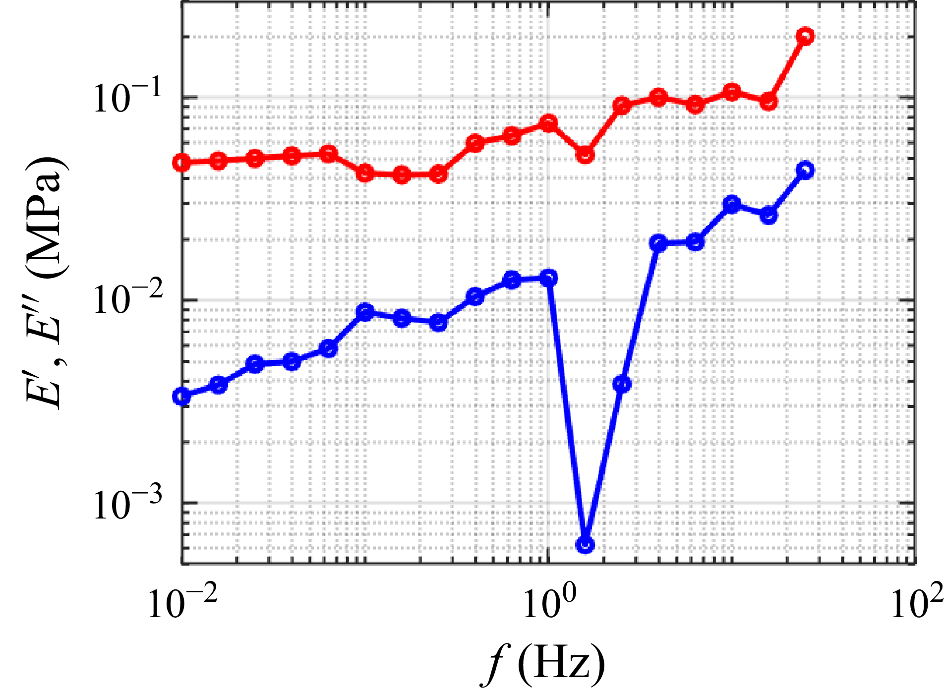
 E′
E′ E″
E″

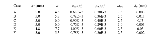

 M∞=2.5
 R=4.5
R=4.5 R=5.3
R=5.3 R=6
R=6 R=6
R=6 M∞=3
M∞=3


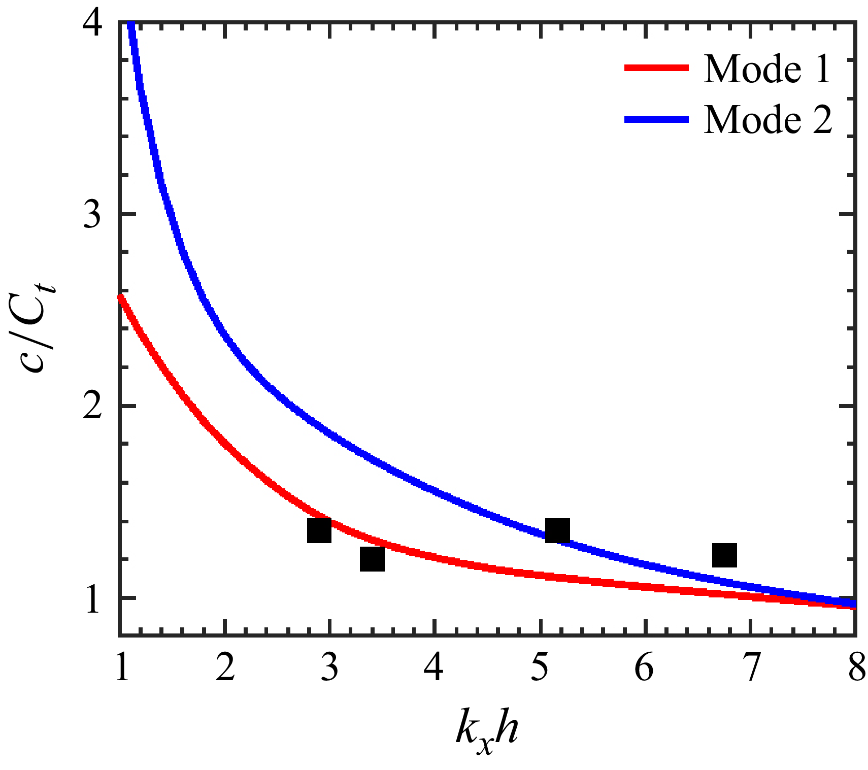


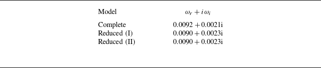

 (ωi
(ωi (ωr
(ωr kxh=2
kxh=2
 vsc
vsc
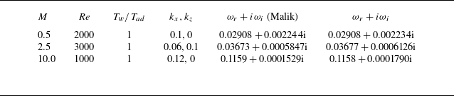

 ωr
ωr kr
kr
 f=900
f=900
 Open access

