


1. Introduction
Wind energy is a crucial renewable energy source for decarbonizing the electricity grid. Investments are focusing on massive off-shore clusters made of increasingly large wind turbines (IRENA 2019). In this context, the wind farm interaction with the atmospheric boundary layer (ABL) has emerged as an increasingly important aspect to account for and model in order to yield accurate power predictions. Its existence uncovered new phenomena that conventional models either fail to capture, such as the wind deceleration upstream of a turbine cluster (Bleeg et al. Reference Bleeg, Purcell, Ruisi and Traiger2018), or model only partially, such as farm-scale wake effects (Nygaard et al. Reference Nygaard, Poulsen, Svensson and Grønnegaard Pedersen2022). The latter are produced by the interacting turbine wakes that merge eventually to form an extended region of reduced momentum downstream of the wind farm. This process, characterized by complex flow dynamics, cannot be described solely by a simple combination of individual wake deficits, but is rather affected by the intricate interplay of additional physical phenomena. First, vertical momentum flux is increased because of the added shear stress created by the wind turbines (Allaerts & Meyers Reference Allaerts and Meyers2017). Second, the wind farm can be seen as a step change in equivalent roughness (Calaf, Meneveau & Meyers Reference Calaf, Meneveau and Meyers2010; Chamorro & Porté-Agel Reference Chamorro and Porté-Agel2011), which leads to the formation of internal boundary layers (IBLs) that grow from the wind farm start and exit (Elliott Reference Elliott1958; Pendergrass & Arya Reference Pendergrass and Arya1984; Savelyev & Taylor Reference Savelyev and Taylor2005). Downstream, it is expected that wake evolution is affected by boundary layer internal stability and enhanced vertical momentum fluxes produced by the augmented shear stress. These are all topics of growing interest for the scientific community as more wind farms are constructed near pre-existing ones (Nygaard et al. Reference Nygaard, Steen, Poulsen and Pedersen2020; Stieren & Stevens Reference Stieren and Stevens2021).
While conventional wake models (Jensen Reference Jensen1983; Ainslie Reference Ainslie1988; Bastankhah & Porté-Agel Reference Bastankhah and Porté-Agel2014; Niayifar & Porté-Agel Reference Niayifar and Porté-Agel2016) look at only the turbine scale, efforts to include some of the large-scale physics have been attempted by Pedersen et al. (Reference Pedersen, Svensson, Poulsen and Nygaard2022) with the introduction of the so-called turbulence-optimized park model. On the other hand, a new class of models has emerged, adopting a ‘coupled’ approach wherein conventional turbine-scale wake models are coupled suitably with additional sub-models aimed at capturing the meso-scale physics that is otherwise absent. This concept, introduced initially by Frandsen et al. (Reference Frandsen, Barthelmie, Pryor, Rathmann, Larsen, Højstrup and Thøgersen2006), was later refined by Stevens, Gayme & Meneveau (Reference Stevens, Gayme and Meneveau2015) as the coupled wake boundary layer model, in which the original top-down model of Calaf et al. (Reference Calaf, Meneveau and Meyers2010) was coupled with a wake model to enhance wind farm power predictions. The top-down model, obtained by balancing horizontally averaged momentum across the wind farm layer, provides an increased equivalent roughness length inside the wind farm, and postulates two equilibrium layers characterized by different values of friction velocities. Although its original formulation assumed a fully developed regime and infinitely large wind farms, the top-down model has been extended later by Meneveau (Reference Meneveau2012) to the wind farm entrance region, where an IBL grows due to the step change in equivalent roughness produced by the wind farm. This updated model was then used by Shapiro et al. (Reference Shapiro, Starke, Meneveau and Gayme2019), and later by Starke et al. (Reference Starke, Meneveau, King and Gayme2021), in their area-localized coupled model. Specifically, both studies apply the top-down model to arbitrary wind farm geometries. While technically the model's derivation justifies its application solely to infinite arrays in the fully developed regime, the authors contend that by considering results as locally averaged and ensuring a wind farm of sufficient size for this horizontal filtering to be meaningful, the top-down parametrization can be extended effectively to arbitrary layouts.
The coupling idea has also been used by Nishino & Dunstan (Reference Nishino and Dunstan2020) to develop a two-scale momentum theory linking conventional momentum theory with the large-scale momentum balance above the wind farm layer. This was later extended by Kirby, Dunstan & Nishino (Reference Kirby, Dunstan and Nishino2023) to predict the power of large wind farms using the unperturbed shear stress profile as input. Finally, Stipa et al. (Reference Stipa, Ajay, Allaerts and Brinkerhoff2023a) introduced recently the multi-scale coupled model to capture global blockage and other free atmosphere stability effects on wind farm performance.
Focusing on the meso-scale side of the problem, it is clear that an accurate parametrization of the shear stress profile evolution within and past the wind farm is crucial to enhance predictions of momentum availability at the large scale. This would allow a more physics-based approach to model the turbulent mixing enhancement produced by wind farms within the coupled class of models. In the present study, we focus our attention on conventionally neutral boundary layers (CNBLs), where a stable free atmosphere characterized by a lapse rate  $\gamma$ and a strong inversion layer with temperature jump $\Delta \theta$ overtops a neutrally stratified layer in which turbulence develops capped by the inversion layer (Zilitinkevich et al. Reference Zilitinkevich, Tyuryakov, Troitskaya and Mareev2012). The wind profile of a CNBL differs from that of a truly neutral boundary layer where stratification is fully absent, in that a deviation from the standard law of the wall and the formation of a super-geostrophic jet have been observed (Kelly, Cersosimo & Berg Reference Kelly, Cersosimo and Berg2019; Liu, Gadde & Stevens Reference Liu, Gadde and Stevens2021).
On the other hand, the influence of internal ABL stability on the shear stress profile has been studied by Nieuwstadt (Reference Nieuwstadt1983), who concluded that the vertical profile of shear stress magnitude approaches the classic linear shape
 \begin{equation} \tau/u^{*2} = 1 - z/H \end{equation}
(where  $H$ is the boundary layer height) for neutral or fully convective conditions, while in stable cases, it exhibits an upward concavity that increases with stability. In particular, Nieuwstadt (Reference Nieuwstadt1984) modelled the stable, nocturnal boundary layer as
 \begin{equation} \tau/u^{*2} = (1 - z/H)^{3/2}. \end{equation}
In CNBLs, only the free atmosphere is thermally stratified, so turbulence develops mainly as in neutral conditions except close to the inversion layer, where buoyancy effects become important. As a consequence, as testified by the large-eddy simulations (LES) conducted by Allaerts & Meyers (Reference Allaerts and Meyers2017), Abkar & Porté-Agel (Reference Abkar and Porté-Agel2013) and Liu et al. (Reference Liu, Gadde and Stevens2021), the shear stress profile is almost linear in its lower part, and transitions smoothly to zero with a mild concavity close to  $H$. Finally, when a wind farm is present within the boundary layer, the shear stress profile retains its self-similarity above the wind farm layer if non-dimensionalized with the friction velocity that characterizes the layer above the wind turbines, referred to as $u^*_{hi}$ (Calaf et al. Reference Calaf, Meneveau and Meyers2010; Kirby et al. Reference Kirby, Dunstan and Nishino2023).
Building on the top-down model of Meneveau (Reference Meneveau2012), we propose here a simple analytical model for the horizontal shear stress components  $\tau _{xz}$ and $\tau _{yz}$ around a large finite-size turbine array. The model is validated against data from LES, and captures the evolution of the horizontal shear stress components in three different flow regions, namely the developing region of the wind farm IBL, the fully developed region (if present), and the wind farm wake.
The present paper is organized as follows. The proposed shear stress model is described in § 2, while § 3 validates the model against LES data presented in Stipa et al. (Reference Stipa, Ajay, Allaerts and Brinkerhoff2023a). Conclusions are finally drawn in § 4, together with notes on future work and the limitations of the present study.
2. Methodology
We assume that the background state existing without the wind farm corresponds to a CNBL of height  $H$, i.e. with neutral stratification below a capping inversion layer centred at $H$. Furthermore, we define $h_{hub}$ and $D$ as the average hub height and turbine diameter within the cluster, while $z_0$ is the unperturbed equivalent roughness height in the absence of any turbine. For simplicity, we assume that the wind is aligned with the $x$ coordinate, while $y$ corresponds to the spanwise direction. Wind farm entrance effects are modelled by considering an IBL of height $\delta _f$ that grows from the start of the wind farm (Chamorro & Porté-Agel Reference Chamorro and Porté-Agel2011; Meneveau Reference Meneveau2012) due to the change in roughness produced by the cluster. In addition, a second IBL, characterized by a height $\delta _w$, grows from the wind farm exit due to the roughness transitioning back to $z_0$. Finally, similarly to Starke et al. (Reference Starke, Meneveau, King and Gayme2021), we assume that the conditions at a given point exclusively depend on the upstream averaged planform wind farm thrust coefficient $c_{ft}$. This in turn depends on the rotor diameter, turbine $C_T$ and spacings $S_x$ and $S_y$, as detailed in § 2.1.
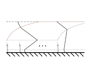
We subdivide the boundary layer structure into four vertically stacked layers, shown in figure 1(a). The ‘low-stress layer’ spans from  $z_0$ to $h_{hub} - D/2$; the ‘wind farm layer’ spans from $h_{hub} - D/2$ to $\delta _w$; the ‘high-stress layer’ spans from $\delta _w$ to $\delta _f$; and the ‘background stress layer’ spans from $\delta _f$ to $H$. The vertical shear stress magnitude profile is assumed to be piecewise linear and continuous at each layer interface. This is a reasonable assumption for truly or conventionally neutral boundary layers, but may be revised in the future for internally stable ABLs where the background shear stress profile depicts an upward concavity (Nieuwstadt Reference Nieuwstadt1984). Analytical expressions within each layer are derived by exploiting the theory developed by Frandsen et al. (Reference Frandsen, Barthelmie, Pryor, Rathmann, Larsen, Højstrup and Thøgersen2006) and later refined by Calaf et al. (Reference Calaf, Meneveau and Meyers2010). Specifically, these authors introduced a relation for the increased wind farm equivalent roughness height $z_{0,{hi}}$, and postulated the existence of constant stress layers below and above the wind turbines, characterized by friction velocities $u^*_{lo}$ and $u^*_{hi}$, respectively. The horizontal shear stress components $\tau _{xz}$ and $\tau _{yz}$ are obtained from the modelled profile of shear stress magnitude by assuming that the shear stress angle profile is unperturbed by the wind farm. Extension of such theory to the wind farm wake is done by assuming an exponential return of $u^*_{lo}$ and $u^*_{hi}$ to the unperturbed friction velocity $u^*$, resulting in a decay of the vertical shear stress profile to its unperturbed shape far downstream. A qualitative sketch of the model is given in figure 1. Note that the height of the wake boundary layer $\delta _w$ is constant and equal to $h_{hub}+D/2$ throughout the wind farm (figure 1a), while the wind farm boundary layer height $\delta _f$ is constant in the wind farm wake. In particular, if a fully developed regime is reached inside the wind farm, then $\delta _f$ coincides with the unperturbed boundary layer height $H$; otherwise, it is set to the value of $\delta _f$ obtained at the wind farm exit.
(a) Sketch of the proposed shear stress profile model inside the wind farm. (b) Qualitative evolution of the vertical profile of shear stress magnitude inside and downwind of the wind farm. Note that  $\delta _w$ is constant and equal to $h_{hub} + D/2$ inside the wind farm.

In our study, we consider  $H$ as constant, neglecting its potential growth from turbulent entrainment at the boundary layer's top and fluctuations caused by atmospheric gravity waves. While, notably, turbulent entrainment affects $H$ if infinite wind farms are considered (Abkar & Porté-Agel Reference Abkar and Porté-Agel2013; Porté-Agel, Bastankhah & Shamsoddin Reference Porté-Agel, Bastankhah and Shamsoddin2020), its resulting growth rate leads to only marginal changes in $H$ over the transit time of a flow particle through a wind farm of finite length. In this case, the more substantial contribution comes from interface waves within the inversion layer and atmospheric gravity waves in the free atmosphere. These waves induce both positive and negative displacements across the wind farm's length, potentially influencing pressure and velocity below the inversion and thereby impacting wind farm power dynamics (Lanzilao & Meyers Reference Lanzilao and Meyers2023; Stipa et al. Reference Stipa, Ajay, Allaerts and Brinkerhoff2023a). Despite its influence on velocity, the inversion displacement caused by gravity waves remains minor compared to the unperturbed $H$, prompting its exclusion from our proposed parametrization.
Overall, the developed model has four free parameters, namely the two friction velocities  $u^*_{lo}$ and $u^*_{hi}$, together with the heights of the two IBLs generated by the step change in roughness, $\delta _f$ and $\delta _w$, growing from the wind farm entrance and exit, respectively. Parametrization of these quantities in the wind farm and the wake regions is described in §§ 2.1 and 2.2.
2.1. Wind farm parametrization
Due to the presence of the wind turbines, the approaching flow experiences a sudden change in equivalent roughness length, which transitions from  $z_0$ to $z_{0,{hi}}$. As a result, an IBL characterized by a height $\delta _f$ grows with increasing distance $x$ from the wind farm entrance. At the same time, friction velocities $u^*_{lo}$ and $u^*_{hi}$ adjust to their fully developed values, obtained when $\delta _f=H$. Different expressions have been proposed for $\delta _f$, obtained using both velocity and shear stress metrics. For instance, Shir (Reference Shir1972) and Allaerts & Meyers (Reference Allaerts and Meyers2017), observed that shear stress adapts faster than velocity to a sudden increase in roughness. In the present study, the IBL height is identified as the vertical location where the relative difference between the actual and unperturbed shear stress magnitude vanishes, and it is modelled following Pendergrass & Arya (Reference Pendergrass and Arya1984), who expressed $\delta _f$ as
 \begin{equation} \delta_f = \text{min}\left[H,z_{tt} + 0.32 z_{0,{hi}} \left(\frac{d_f}{z_{0,{hi}}}\right)^{0.8}\right], \end{equation}
where  $z_{tt}$ is the average top-tip height, and $d_f$ is the distance from the wind farm start. The increased equivalent roughness height is given by
 \begin{align} z_{0,{hi}} = h_{hub} \left(1 + \frac{D}{2h_{hub}}\right)^\beta \exp \left[-\left(\frac{\widetilde{c_{ft}}}{2\kappa^2}+\left[\ln\left(\frac{h_{hub}}{z_0} \left(1-\frac{D}{2h_{hub}}\right)^\beta\right)\right]^{{-}2}\right)^{{-}1/2}\right], \end{align}
where  $\beta =\nu ^*_w/(1+\nu ^*_w)$ is evaluated using $\nu ^*_w \approx 28\sqrt {0.5\widetilde {c_{ft}}}$ (see Calaf et al. (Reference Calaf, Meneveau and Meyers2010) for details). Note that $\delta _f$, $z_{0,{hi}}$, $\beta$ and $\nu ^*_w$ are all functions of position $\boldsymbol {x}$, but such dependency has been dropped for ease of notation. The parameter $\widetilde {c_{ft}}$ (also a function of position) can be evaluated by averaging the wind farm thrust coefficient per unit area $c_{ft}$ upwind with respect to location $\boldsymbol {x}$ and along a streamline through the point of interest, assumed in the present study to be rectilinear. Following Starke et al. (Reference Starke, Meneveau, King and Gayme2021), we argue that such an averaging procedure better represents the fact that the IBL height at any $x$ depends on the thrust coefficient per unit area experienced up to that point rather than on its local value. In order to perform the averaging operation, $c_{ft}$ is defined at every cell of a two-dimensional Cartesian sampling grid as
 \begin{equation} c_{ft}^{ij} = {\rm \pi}C_T\,\frac{D^2}{4S_x^{ij}S_y^{ij}} , \end{equation}
where  $C_T$ is the thrust coefficient of the closest turbine, while $S_x^{ij}$ and $S_y^{ij}$ are the streamwise and spanwise turbine spacings at a given cell. Their values are obtained as follows. First, for each turbine, we define $x$ and $y$ stripes characterized by a two diameters width, whose axis of symmetry passes through the turbine base location. Then streamwise and spanwise spacings $S_x$ and $S_y$ associated with the wind turbine of interest are found by looking for its closest rotor belonging to the $x$ and $y$ stripes, respectively (figure 2a). To transfer such information to the sampling grid, we first find the wind turbine closest to each grid cell, then set $S_x^{ij}$ and $S_y^{ij}$ to the values associated with the closest turbine. In doing so, if the closest turbine lies outside of the grid cell, then $S_x^{ij}$ and $S_y^{ij}$ are set to infinity, so that $c_{ft}^{ij}$ approaches zero (no wind turbines are in the cell). The grid spacings along $x$ and $y$ are set to the maximum between $S_x$ and $S_y$ among all turbines in the cluster. This approach resembles that of Starke et al. (Reference Starke, Meneveau, King and Gayme2021), who used a Voronoi tessellation that assigns a triangular grid cell to each wind turbine, but leaves the wind farm wake uncovered by the tessellation. Since in our approach we are interested in not only the shear stress within the wind farm but also its downstream evolution, a Cartesian grid is the simplest and most natural choice to achieve this objective.
(a) Sketch of the turbine spacing evaluation algorithm. In yellow and green are the stripes to select those turbines that should be used for computing streamwise and spanwise spacing, respectively. (b) Sketch of the ray-casting procedure to evaluate  $\widetilde {c_{ft}}^{ij}$ at the cell of interest from the $c_{ft}$ field defined on the sampling grid. This procedure is also used to infer the start and ending coordinates of the wind farm.

Once  $c_{ft}^{ij}$ is known, the upwind-averaged $\widetilde {c_{ft}}^{ij}$ can be evaluated by casting a ray directed upwind from the cell centre of interest (figure 2b), and averaging $c_{ft}^{ij}$ on the ray. In this regard, three cases are possible. If the query point is upwind of the wind farm, then $\widetilde {c_{ft}}^{ij}$ is set to zero. If the query point is inside the wind farm, then $\widetilde {c_{ft}}^{ij}$ is set to the average $c_{ft}$ on the ray from the wind farm start up to the query point. Finally, if the point lies within the wind farm wake, then $\widetilde {c_{ft}}$ is set to the average $c_{ft}$ on a ray spanning the whole wind farm. In the latter case, the resulting $\widetilde {c_{ft}}$ corresponds to the value at the wind farm exit, used to compute $u^*_{lo}$ and $u^*_{hi}$ at the same location. Then an exponential decay will be applied to model a partial return of $u^*_{lo}$ and $u^*_{hi}$ to their equilibrium values (this is explained in more detail in § 2.2). To detect the point location with respect to the wind farm, we use the $c_{ft}$ field itself. In fact, as it goes from zero to a positive value, query points will be inside the wind farm until $c_{ft}$ goes back to zero. Conversely, after the latter condition is verified, points will be located in the wake. The same argument can be used to infer the distance of any given point $\boldsymbol {x}$ from the wind farm start or exit. Note that the above algorithm treats each ray – or streamwise stripe of cells – as if it were infinite in the spanwise direction, so that there is no mutual interaction between adjacent strips. Starke et al. (Reference Starke, Meneveau, King and Gayme2021) made the same approximation, which is justified in our case by the fact that the proposed model already filters the actual shear stress profiles by smoothing the thrust coefficient per unit area over the Cartesian cells.
Once  $z_{0,{hi}}$ and $\delta _f$ are known at any grid cell, friction velocities $u^*_{lo}$ and $u^*_{hi}$ can be evaluated as
 \begin{gather} u^*_{hi} = u^*\,\frac{\ln\left(\dfrac{\delta_f}{z_0}\right)}{\ln\left(\dfrac{\delta_f}{z_{0,{hi}}}\right)}, \end{gather}
 \begin{gather}u^*_{lo} = u^*_{hi}\,\frac{\ln\left[\dfrac{h_{ref}}{z_{0,{hi}}}\left(1+\dfrac{D}{2h_{ref}}\right)^\beta\right]}{ \ln\left[\dfrac{h_{ref}}{z_0}\left(1-\dfrac{D}{2h_{ref}}\right)^\beta\right]}. \end{gather}
Finally, after having introduced  $\tau _{w,lo} = u^{\ast 2}_{lo}$, $\tau _{w,hi} = u^{\ast 2}_{hi}$ and $\tau _{{w},\infty } = u^{\ast 2}$, the vertical profile of shear stress magnitude can be fully defined at every cell in each layer as
 \begin{equation} \tau_{lsl} = \tau_{w,lo}\left(1-\frac{h}{H}\right), \quad h \leq z_{bt}\quad(\mbox{low-stress layer}),\end{equation}
 \begin{align} \tau_{wfl} &=\frac{h-z_{tb}}{z_{tt}-z_{tb}}\left[\tau_{w,lo}\left(\frac{z_{tb}}{H}-1\right) + \tau_{w,hi}\left(1-\frac{z_{tt}}{\delta_f}\right)+\tau_{{w},\infty}\left(\frac{z_{tt}}{\delta_f}-\frac{z_{tt}}{H}\right) \right]\nonumber\\ &\quad + \tau_{w,lo}\left(1-\frac{z_{tb}}{H}\right), \quad z_{bt} < h \leq \delta_w\quad(\mbox{wind farm layer}), \end{align}
 \begin{gather} \tau_{hsl} = \frac{h}{\delta_f}\left[\tau_{{w},\infty}\left(1-\frac{\delta_f}{H}\right)-\tau_{w,hi}\right] + \tau_{w,hi},\quad \delta_w < h \leq \delta_f\quad(\mbox{high-stress layer}),\end{gather}
 \begin{gather} \tau_{bsl} = \tau_{{w},\infty}\left(1-\frac{h}{H}\right),\quad \delta_f < h \leq H\quad(\mbox{background stress layer}),\end{gather}
where  $z_{bt}$ and $z_{tt}$ are the turbine bottom-tip and top-tip heights, respectively. The resulting profile, depicted in figure 1(a), is piecewise linear and continuous at the layer heights. Note that the background stress layer is present only in the developing region of the wind farm IBL, while it disappears once $\delta _f=H$. Conversely, the high-stress layer is non-existent at the wind farm start where $\delta _f=z_{tt}$.
2.2. Wake parametrization
At the wind farm exit, another discontinuity in roughness height is encountered from  $z_{0,{hi}}$ to $z_0$. As a consequence, a second IBL will start growing, while $u^*_{lo}$ and $u^*_{hi}$ will return slowly to the unperturbed friction velocity $u^*$ as
 \begin{gather} u^*_{hi} = [1-\exp({-}d_w/L)]u^* + \exp({-}d_w/L)u^*_{hi,e}, \end{gather}
 \begin{gather}u^*_{lo} = [1-\exp({-}d_w/L)]u^* + \exp({-}d_w/L)u^*_{lo,e}, \end{gather}
where  $d_w$ is the distance from the wind farm exit of the query point, $u^*_{hi,e}$ and $u^*_{lo,e}$ are the friction velocities obtained at the wind farm exit, and $L$ is a length scale related to the turbulence decay. In the present study, we fix $L$ to $5$ km, which is expected to hold for neutral CNBLs and a background roughness close to the value reported in table 1. This provided the highest agreement with our LES results.
Input parameters for the wind farm simulations.

For instance, Cañadillas et al. (Reference Cañadillas2020) developed an analytical model to predict velocity in the wake and used the time scale
 \begin{equation} T = \frac{\varPhi(\xi)\,D^2}{\kappa u^* z_{hub}} , \end{equation}
where  $\varPhi (\xi )$ is the non-dimensional wind shear, a function of the Monin–Obukhov similarity parameter $\xi$ inside the boundary layer (Stull Reference Stull1988). One interesting aspect that can be observed is that the time scale for velocity recovery does not depend on the wind farm length. Moreover, as pointed out by Cañadillas et al. (Reference Cañadillas2020), shear stress and velocity are tightly related in the wind farm wake, so the same finding can be expected for the recovery of shear stress. Specifically, while it is true that the wind farm length determines how much shear stress can evolve before leaving the cluster, its recovery is expected to depend only on general wind turbine characteristics, internal ABL stability and equivalent roughness height. However, as mentioned by Allaerts & Meyers (Reference Allaerts and Meyers2017), shear stress adapts faster than velocity to changes in equivalent roughness. This can be observed also in Bastankhah et al. (Reference Bastankhah, Mohammadi, Lees, Diaz, Buxton and Ivanell2023) and may lead to a slightly different recovery time scale between these two quantities. Therefore, although in general we expect $L$ to have a similar functional relationship with (2.12) – of course, after multiplying by a suitable mean advection velocity – this requires further investigation and has not been addressed in the present paper. Downstream of the wind farm, the IBL growth is approximated as
 \begin{equation} \delta_w = \text{min}\left[H,z_{tt} + 0.32 z_0 \left(\frac{d_w}{z_0}\right)^{0.8}\right], \end{equation}
again following Pendergrass & Arya (Reference Pendergrass and Arya1984). Its effect is to raise the top of the wind farm layer until it reaches the unperturbed boundary layer height  $H$. In order to compute the shear stress, (2.6)–(2.9) still hold upon substituting $z_{tt}$ with $\delta _w$, as the wind farm layer does not have a constant thickness downstream of the cluster (see figure 1b).
3. Results
In this section, we validate the proposed model for the vertical shear stress profile against LES conducted with TOSCA (Toolbox fOr Stratified Convective Atmospheres). TOSCA solves the incompressible Navier–Stokes equations, formulated in generalized curvilinear coordinates, exploiting the finite-volume method. Details about the code and its validation are provided in Stipa et al. (Reference Stipa, Ajay, Allaerts and Brinkerhoff2023b). The two LES cases differ only in the prescribed capping inversion strength, and correspond to the subcritical and supercritical conditions presented in Stipa et al. (Reference Stipa, Ajay, Allaerts and Brinkerhoff2023a). Our choice to vary the inversion strength is justified by results from Lanzilao & Meyers (Reference Lanzilao and Meyers2023), where  $\Delta \theta$ emerges as the main parameter influencing wind farm flows under stratified free atmosphere, together with the lapse rate $\gamma$ and inversion height $H$. The wind farm consists of 100 NREL 5 MW wind turbines (Jonkman et al. Reference Jonkman, Butterfield, Musial and Scott2009), organized in 20 rows and 5 columns. Streamwise and spanwise turbine spacings are set to $630$ m and $600$ m, respectively. To prescribe a realistic turbulent inflow condition to the wind farm, we use the hybrid offline/concurrent precursor technique described in Stipa et al. (Reference Stipa, Ajay, Allaerts and Brinkerhoff2023b). The offline precursor has been carried out for $100\ 000$ s, while the successor phase of the analysis lasted for $20\ 000$ s. Statistics are gathered for the last $15\ 000$ s of simulation. Input parameters for the ABL are reported in table 1, where $\theta _0$ and $\Delta h$ are the ground potential temperature and inversion width, respectively, that are used together with $\Delta \theta$, $\gamma$ and $H$ to initialize the background potential temperature profile with the model proposed by Rampanelli & Zardi (Reference Rampanelli and Zardi2004). The parameter $u_{ref}$ is the average wind at $h_{ref}$ (chosen as the wind turbine hub height), while $z_0$ is the equivalent roughness length. Further details on the simulation set-up are given in Stipa et al. (Reference Stipa, Ajay, Allaerts and Brinkerhoff2023a).
Regarding the shear stress model, we calculate the unperturbed shear stress angle profile from the LES, but this can also be evaluated using e.g. the model proposed by Nieuwstadt (Reference Nieuwstadt1983). Moreover, wind turbine  $C_T$ resulting from the LES is fairly constant throughout the wind farm as all turbines operate below rated conditions. Hence for the shear stress model we assume $C_T=0.85$ for all turbines in the present study, which results in a constant $c_{ft}$ field equal to $0.028$ throughout the wind farm. We highlight that the procedure presented in § 2.1 to compute the $c_{ft}$ field does not impose any restriction on the wind farm geometry, except that the wind farm has to be large enough to produce perturbations in shear stress when this is averaged around the location of interest. Figure 3 shows the $c_{ft}$ field corresponding to the wind farm object of the present study. Specifically, this is finite in both the spanwise and streamwise directions.
Contour of the  $c_{ft}$ field resulting from applying the algorithm presented in § 2.1. Red circles identify the wind turbine locations.

Figure 4 compares profiles of  $\tau _{xz}$ and $\tau _{yz}$ from the two LES. Data have been spanwise-averaged from $y=0$ to $y=3000$, corresponding to the wind farm spanwise envelope. Surprisingly, the variation in inversion strength between the two cases does not impact the shear stress profile evolution within or beyond the wind farm. This suggests that also free atmosphere stratification aloft, typically weaker than the stability found in the inversion layer, might not affect the shear stress disturbances caused by the wind farm. In light of these observations, while stability within the inversion and in the free atmosphere have large implications in the wind speed dynamics (Allaerts & Meyers Reference Allaerts and Meyers2017; Lanzilao & Meyers Reference Lanzilao and Meyers2023; Stipa et al. Reference Stipa, Ajay, Allaerts and Brinkerhoff2023a), we argue that the physics of shear stress perturbations seems mainly confined to the boundary layer flow, thus justifying the absence of a free atmosphere parametrization in the proposed model. Conversely, internal ABL stability is expected to play an important role, and this is a subject for further investigation. Looking at figure 4, it can be seen how the peak in $\tau _{xz}$ is located at $z_{tt}$ inside the wind farm, while it shifts upwards in the wind farm wake, where the shear stress returns slowly to its equilibrium value. Finally, the growth of $\delta _f$ is clearly visible, as the height at which the local profile differs from the free-stream increases with downstream distance from the wind farm entrance.
Comparison of shear stress profiles between the two LES for different locations inside the wind farm (identified by the row number) and in the wind farm wake (identified by the distance in diameters from the wind farm exit). Red indicates  $\Delta \theta =7.312$; blue indicates $\Delta \theta =4.895$; horizontal dotted lines indicate top and bottom turbine tip heights.

Figure 5 compares profiles of  $\tau _{xz}$ and $\tau _{yz}$ resulting from the proposed model against their LES predictions from the two simulations. Also in this case, LES data have been averaged along the spanwise direction from $y=0$ to $y=3000$. For reference, we also show in each plot the free-stream shear stress magnitude profile $\tau _\infty$, evaluated from LES. It can be noticed how the model predictions agree well with the LES results, both inside and downstream of the wind farm for the two simulated cases. Moreover, the assumption that the wind farm does not perturb the initial shear stress angle profile significantly is verified, as both profiles of $\tau _{xz}$ and $\tau _{yz}$ predicted by the model are in strong agreement with the LES data, especially in the fully developed region. Here, the maximum value of $\tau _{xz}$ is around three times $\tau _{{w},\infty }$, meaning that vertical momentum fluxes are strongly enhanced by the presence of the wind farm. In the developing region, especially where $\delta _f$ approaches $H$, the shear stress profile evaluated from the LES exhibits an upward concavity close to $H$, slightly disagreeing with the piecewise linear approximation. This effect could be due to non-negligible thermal and non-equilibrium effects that may affect the shear stress profile near $H$ in the region where the flow transitions to a fully developed regime. Nevertheless, the piecewise linear assumption describes satisfactorily the features of the shear stress profile in all regions on the flow, with the highest agreement found in the wind farm wake and in the fully developed region.
Comparison between the proposed model and LES results for different locations inside the wind farm (identified by the row number) and in the wind farm wake (identified by the distance in diameters from the wind farm exit) for (a)  $\Delta \theta =7.312$ and (b) $\Delta \theta =4.895$. Horizontal dotted lines indicate top and bottom turbine tip heights.

In order to assess the accuracy of the methodology used to compute  $u^*_{lo}$, $u^*_{hi}$, $\delta _f$ and $\delta _w$, we performed a least squares fit of the shear stress magnitude profile obtained from the LES with its piecewise linear shape assumed in the proposed model. In particular, we left $u^*_{lo}$, $u^*_{hi}$, $\delta _f$ and $\delta _w$ free to be determined by the least squares fit operation. Results for the $\Delta \theta =7.312$ case are shown in figure 6, where we report $u^*_{lo}$, $u^*_{hi}$, $\delta _f$ and $\delta _w$ evaluated using both the least squares fit and the equations reported in § 2. The same analysis for the $\Delta \theta =4.895$ case points to similar conclusions, hence it is not reported. Referring to figure 6, while very good agreement can be found in the friction velocities $u^*_{lo}$ and $u^*_{hi}$, the least squares fit predicts a slower growth of the wind farm IBL than (2.1). This can be confirmed also by looking at the developing region in figure 5, i.e. from row 1 to row 8. Conversely, good agreement is found when analytical predictions of $\delta _f$ are compared against data obtained from LES by using the following criterion. At each streamwise location, we first look for the height where the difference between the actual and unperturbed stress is less than 5 % of $u^{\ast 2}$. Then $\delta _f$ is extrapolated as the height where such difference is zero. Such a criterion, depicted in red in figure 6, predicts a faster growth of $\delta _f$ if compared with the least squares fit. A possible reason is that within the developing region, the shear stress profile in the high-stress layer is not strictly linear but instead features the upward concavity mentioned above. As a consequence, minimizing the least squares error within the whole layer or adopting the proposed criterion locally yields differences in the shear stress slope, reflected in slightly distinct $\delta _f$ predictions. Conversely, the analytical growth of the wake IBL given by (2.13) follows closely the least squares fit obtained in the wind farm wake, supporting our choice to model the upward shift of the wind farm layer top. This allows the model to capture the upward displacement of the shear stress peak located initially at $z_{tt}$ at the wind farm exit.
Comparisons between values of (a)  $u^*_{hi}$ and $u^*_{lo}$, and (b) $\delta _f$ and $\delta _w$, obtained using the formula of Pendergrass & Arya (Reference Pendergrass and Arya1984) and as a result of fitting LES results with the assumed shear stress model shape in a least squares sense (LES fit). The red line in (b) corresponds to $\delta _f$ evaluated from LES data using the criterion explained in the text (LES).

Finally, figure 7 compares different analytical formulations for the IBL growth (see Savelyev & Taylor (Reference Savelyev and Taylor2005) for a review) against LES data already shown in figure 6. Also in this case, we show only data from the case characterized by  $\Delta \theta =7.312$. All studies approximate $\delta$ as
 \begin{equation} \frac{\delta}{z_{0,D}} = \frac{\delta(0)}{z_{0,D}} + A\left(\frac{x}{z_{0,D}}\right)^{0.8} , \end{equation}
where  $z_{0,D}$ is the roughness height downstream of the discontinuity. In particular, it can be noticed how, for both $\delta _f$ and $\delta _w$, the formulas of Elliott (Reference Elliott1958) and Meneveau (Reference Meneveau2012) predict a faster IBL growth than what is observed in our numerical simulations, as they assume $A=0.75+0.03\ln (z_{0,D}/z_{0,U})$ and $A=1.0$, respectively, where $z_{0,U}$ is the roughness height upwind of the discontinuity. For this reason, we used the analytical formulation of Pendergrass & Arya (Reference Pendergrass and Arya1984), who estimated $A=0.32$. The same observation was also made by Allaerts & Meyers (Reference Allaerts and Meyers2017), who estimated $\delta _f$ as $\delta _f(0)+0.57x^{0.74}$. For instance, this result agrees well with the wind farm IBL predicted by fitting the LES data with the shear stress model shape, suggesting that further research may be needed to fully understand wind farm IBL growth.
Comparison of (a) wind farm IBL  $\delta _f$ and (b) wake IBL $\delta _w$ obtained using different analytical formulas and as calculated by fitting LES data with the assumed shape for the vertical profile of shear stress magnitude (LES fit). For $\delta _f$, results obtained with the criterion explained in the text (LES) and from the Allaerts & Meyers (Reference Allaerts and Meyers2017) formula are also shown.

4. Conclusions
In the present study, we introduced an analytical model to predict the vertical profiles of shear stress magnitude for the flow around a finite-size wind farm in a conventionally neutral boundary layer. The model has been validated against LES results, and proved to capture accurately the growth of the wind farm IBL, the shear stress profile in the developing and fully developed region, as well as the return to equilibrium of the shear stress components in the wind farm wake, where the growth of a second IBL is observed. The suite of LES cases revealed that the shear stress is not influenced by the strength of the inversion layer, suggesting that its shape and evolution may not be influenced by free atmosphere stratification. Moreover, the assumption that the vertical profile of shear stress angle is negligibly perturbed by the wind farm is well verified if stress components obtained from the LES are compared against the shear stress magnitude from the model, projected with the unperturbed angle profile resulting from the LES. The model features four free parameters, namely the height of the two IBLs within and downstream of the wind farm,  $\delta _f$ and $\delta _w$, respectively, and the friction velocities $u^*_{lo}$ and $u^*_{hi}$ in the layers of constant stress postulated by Calaf et al. (Reference Calaf, Meneveau and Meyers2010), below and above the wind turbines, respectively. While $u^*_{lo}$ and $u^*_{hi}$ are found analytically using the top-down model (Meneveau Reference Meneveau2012), $\delta _f$ and $\delta _w$ are evaluated using the formula proposed by Pendergrass & Arya (Reference Pendergrass and Arya1984), which predicts a slower IBL growth than the expression from Meneveau (Reference Meneveau2012). Ultimately, these four parameters define the vertical profile of shear stress magnitude, whose shape is postulated. To assess the accuracy of the top-down model, we fitted the shear stress profiles obtained from LES with the shape assumed by the model, and similar values for $u^*_{lo}$, $u^*_{hi}$, $\delta _f$ and $\delta _w$ have been found.
Further research is needed to assess the dependency of the length scale  $L$ used to control the turbulence decay in the wind farm wake, in particular studying its dependence on boundary layer internal stability. In the latter case, the assumed piecewise shape of the shear stress profile should also be verified. Moreover, to assess the accuracy of the model with different levels of background shear stress, we plan to extend the suite of validation to different values of equivalent roughness length.
Overall, we believe that the developed shear stress model provides an important advancement in modelling the increase in shear stress within large finite-size wind farms, enabling a better understanding of its effects by providing a simple yet comprehensive formulation to model vertical momentum fluxes at a given height within the boundary layer.
Funding
The present study is supported by UL Renewables and the Natural Science and Engineering Research Council of Canada (NSERC) through Alliance grant no. 556326. Computational resources provided by the Digital Research Alliance of Canada (www.alliancecan.ca) and Advanced Research Computing at the University of British Columbia (www.arc.ubc.ca) are gratefully acknowledged.
Declaration of interests
The authors report no conflict of interest.


 Open access