


1. Introduction
Gravity-driven flows of one fluid over another can involve complex interactions between the two fluids, which can lead to a rich dynamic behaviour. Such flows occur in a wide range of natural and human-made systems, as in lava flow over less viscous lava (Balmforth et al. Reference Balmforth, Burbidge, Craster, Salzig and Shen2000; Griffiths Reference Griffiths2000), spreading of the lithosphere over the mid-mantle boundary (Lister & Kerr Reference Lister and Kerr1989; Dauck et al. Reference Dauck, Box, Gell, Neufeld and Lister2019), ice flow over an ocean (Kivelson et al. Reference Kivelson, Khurana, Russell, Volwerk, Walker and Zimmer2000; DeConto & Pollard Reference DeConto and Pollard2016) and over bedrock covered with sediment and water (Fowler Reference Fowler1987; Stokes et al. Reference Stokes, Clark, Lian and Tulaczyk2007), flows in porous media (Woods & Mason Reference Woods and Mason2000), and droplet motion on liquid-infused surfaces (Keiser et al. Reference Keiser, Keiser, Clanet and Quéré2017).
The flow of GCs in a circular geometry has been studied with a range of boundary conditions. In the absence of a lubricating layer, a common boundary condition along the base of a sole GC is no slip. Such GCs of Newtonian fluids that are discharged at constant flux follow a similarity solution, in which the front position at time  $t$ is proportional to $t^{1/2}$ (Huppert Reference Huppert1982). Similar GCs of power-law (PL) fluids having exponent $n$, where $n=1$ represents a Newtonian fluid and $n>1$ represents a strain-rate softening fluid, also have similarity solutions, in which the front propagation is proportional to $t^{(2n+2)/(5n+3)}$ (Sayag & Worster Reference Sayag and Worster2013).
At the other extreme, the presence of a lower fluid layer can significantly reduce friction at the base of the top fluid, which results in extensionally-dominated GCs. This is the case, for example, for ice shelves, which deform over the relatively inviscid oceans with weak friction along their interface. The late-time front evolution of such axisymmetric GCs of Newtonian fluids is proportional to  $t$ (Pegler & Worster Reference Pegler and Worster2012). However, when the top fluid is strain-rate softening, an initially axisymmetric front can destabilise and develop fingering patterns that consist of tongues separated by rifts (Sayag & Worster Reference Sayag and Worster2019).
In the more general case, friction along the boundaries of the GCs can vary spatiotemporally as their stress field evolves. For example, the interface of an ice sheet with its underlying bed rock can include distributed melt water and sediments, which impose non-uniform and time-dependent friction along the ice base, and evolve spatiotemporally under the stresses imposed by the ice layer (Fowler Reference Fowler1981; Schoof & Hewitt Reference Schoof and Hewitt2013). Consequently, the coupled ice–lubricant system may evolve various flow patterns, such as ice streams (Stokes et al. Reference Stokes, Clark, Lian and Tulaczyk2007) and glacier surges (Fowler Reference Fowler1987). Such systems have been modelled as two coupled GCs of Newtonian fluids spreading one on top of the other (Kowal & Worster Reference Kowal and Worster2015). The early stage of these flows follows a self-similar evolution, in which the fronts of the two fluids evolve like  $t^{1/2}$, as in non-lubricated (no-slip) GCs, and they can have a radially non-monotonic thickness. However, experiments showed that, at a later stage, these coupled flows became unstable and developed fingering patterns and non-axisymmetric flow (Kowal & Worster Reference Kowal and Worster2015). It has been suggested that such instabilities appear when the jump in hydrostatic pressure gradient across the lubrication front is negative (Kowal & Worster Reference Kowal and Worster2019).
Despite the wide range of natural lubricated GCs that involve non-Newtonian fluids, the radial flow of a non-Newtonian fluid over a lubricated layer of a Newtonian fluid has not been explored thus far. In this study, we begin to explore such flows by experimentally investigating the flow of a strain-rate softening fluid that is lubricated by a Newtonian fluid, in a similar setting as in Kowal & Worster (Reference Kowal and Worster2015). We focus on flows that are axisymmetric to the leading order, and explore the case where the flux and viscosity of the lubricating fluid are much smaller than those of the non-Newtonian top fluid. We trace the evolution of the two fronts, and the spatiotemporal evolution of the light transmitted through the two fluids, from which we resolve the thickness distribution of the top-layer, non-Newtonian fluid. We then contrast our findings with the present theories of non-lubricated and lubricated GCs.
2. Experimental set-up
The experimental apparatus (figure 1a,b) included a flat, optically-transparent square glass sheet of  $1\times 1$ m $^2$ and a thickness of 10 mm, supported by an aluminum frame parallel to the ground with an alignment accuracy of 50 micron m $^{-1}$. A rectangular plane mirror was placed underneath the glass sheet at an angle of 45 $^\circ$ to the horizontal for imaging. The centre of the glass sheet had a 5 mm diameter nozzle that was connected to a syringe pump (NE4000) that delivered, at constant flux $Q_\ell$, the Newtonian lubricating fluid of viscosity $\mu _\ell$ and density $\rho _\ell$.
(a) Our experimental apparatus for lubricated GCs. (b) Close-up of the flow region (dash-line rectangle in (a)). (c) Viscosity measurements as a function of strain rate ( $\bullet$, $\circ$) of 1 % (blue) and 2 % (red) of xanthan solutions and the regression to power-law functions ( $\cdot \cdot \cdot\ \cdot$). Inset shows two sets of typical viscosity measurements for each fluid concentration, in which the strain rate varies between 0.001 and 0.007 s $^{-1}$ in steps of 0.002 ${\rm s}^{-1}$, and at each step, the viscosity is measured continuously until an equilibrium value is reached.

The non-Newtonian fluid of viscosity  $\mu$ and density $\rho$ was driven at constant flux $Q$ by gravity from a beaker that was supported by an $xyz$-translation stage through an 8 mm diameter aluminum tube, whose outlet was 15 mm over the glass surface (figure 1a,b). We kept the flux constant by keeping a constant fluid level in the beaker using a peristaltic pump that supplied fluid from a reservoir. A $1\times 1$ m $^2$ white light-sheet and a diffuser were positioned parallel to the glass surface and approximately 50 mm over it to illuminate the flow uniformly. A time-lapsed image sequence was captured throughout each experiment using a Nikon D5500 camera that was facing the 45 $^\circ$ mirror.
2.1. Preparation and properties of the experimental fluids
The non-Newtonian fluid we used was an aqueous solution of food-grade xanthan gum (Jungbunzlauer) of 1 % and 2 % concentration (per weight). To prepare uniformly-dissolved and air-bubble-free solutions, we followed the following procedure: first, we generated a smooth vortex (Eurostat-200) in a beaker containing deionised water. Then, we poured the xanthan-gum powder into the centre of the vortex within less than 60 s, to ensure uniform dispersion of the powder and prevent aggregates before the viscosity of the solution soared. After 90 min of mixing, we added 0.3 g of lemon-yellow colour per 5000 g of solution, and stirred for an additional 30 min. Finally, we stored the solution in a 4  $^\circ$C refrigerator for 24 h to remove residual air bubbles. The densities of the solutions were $1.0035\pm 0.0005$ and $1.007\pm 0.0005$ g cm $^{-3}$ for the 1 % and 2 % concentrations, respectively.
The rheology of xanthan gum solutions of such concentrations has been studied extensively in various flow configurations, and we have described it in detail in Sayag & Worster (Reference Sayag and Worster2019). In general, such xanthan solutions are viscoelastic. However, in flows such as those we consider here, the role of elastic deformation is significantly smaller compared with viscous deformation (e.g. Sayag & Worster Reference Sayag and Worster2013, Reference Sayag and Worster2019), as implied from the small Deborah number that we estimate in § 4. Therefore, here we focus on the viscous deformation of our xanthan solutions, which is known to be consistent with a PL fluid of both shear and extensional thinning for a wide range of strain rates, with an approximately similar exponent (Martín-Alfonso et al. Reference Martín-Alfonso, Cuadri, Berta and Stading2018).
We used TA DHR-3 and ARES rheometers to measure the dependence of the shear viscosity  $\mu$ of our xanthan solutions on the shear rate $\dot {\epsilon }$. The setup consisted of a steady shear flow within a 2 $^\circ$ cone-and-plate geometry (40 mm (DHR-3) and 50 mm (ARES)) and a solvent trap to minimise dehydration. The rate of shear was varied in discrete increasing steps, and the duration of the viscosity measurements at each step was sufficiently long to ascertain that a steady value was reached within a $1\,\%$ standard deviation (STD) (figure 1c, inset). We observed that the viscosity equilibration time was shorter when the shear-rate difference between two consecutive steps was smaller, and when the imposed shear rate was larger. At very low shear rates, the equilibration time was substantial but, at shear rates larger than 0.01 ${\rm s}^{-1}$, the equilibration time was negligible. Fitting our measured viscosity to the power-law relation
 \begin{equation} \mu=k \dot{\epsilon}^{{1/ n}-1}, \end{equation}
while keeping the consistency  $k$ and the exponent $n$ as free parameters, we find that
where each uncertainty represents one STD in the measured quantity (figure 1c).
For a Newtonian lubricating fluid of larger density and lower viscosity, we dissolved glucose in distilled water ( $\approx$38 % glucose in weight) to obtain a solution of density $\rho _\ell =1.164\pm 0.0005$ g cm $^{-3}$ and of dynamic viscosity $\mu _\ell =9.1\pm 0.12$ mPa s at $20\,^\circ$C. We dyed the lubricating fluid in blue ( $0.5\,\%$ per weight) to achieve a high contrast of the evolving fluid–fluid interface and to more easily resolve the evolving thickness of the non-Newtonian fluid layer, as discussed in § 3.2.
2.2. Experimental procedure and preliminary experiments
Two preparation procedures had a major impact on the reproducibility of our experiments. The first was the concentric alignment of the two outlet nozzles of the discharged fluids to an accuracy of  $\pm$100 $\mathrm {\mu }$m. This was done using an acrylic cylindrical adapter that had a circular cavity at one base, concentric with a circular protrusion at the opposite base, which respectively were fitted to the outer diameter of the tube delivering the non-Newtonian fluid and to the inner diameter of the nozzle in the glass surface that delivered the lubricating fluid. The adapter was initially placed over the glass substrate with its protrusion connected to the lower nozzle. Then the $xyz$-stage was lowered ( $z$ direction) so that the feeding tube of the non-Newtonian fluid approached the adapter, and was tuned horizontally ( $x$-
$x$- $y$ directions) to fit the tube into the cavity in the adapter. The calibration was completed when the two nozzles were simultaneously connected to the adapter, at which point the stage was lifted ( $z$ direction) and the adapter was removed. The second procedure concerns the impact of the wetting conditions over the glass surface on the shape of the lubricating-fluid front. In the absence of the non-Newtonian fluid, the axisymmetry of the lubricating-fluid front was sensitive to the wetting conditions of the glass surface. We reduced this sensitivity to the level that the axisymmetric shape of the lubricating-fluid front persisted, by forming uniform wetting conditions over the glass surface using a coating of soap solution (3.3 % liquid dish soap in deionised water) that was allowed to dehydrate prior to the initiation of our experiments. To verify that the soap coating had no impact on the non-Newtonian GC, we compared the front evolution of a non-lubricated GCs with and without a soap coating, and found no measurable difference for xanthan concentrations of either 1 % or 2 % (figure 2a). A possible cause for the difference in sensitivity to the wetting conditions between the two fluids is the large ( $\approx$16) Bond number of the non-Newtonian fluid and the relatively small ( $\approx$0.03) Bond number of the lubricating Newtonian fluid. We elaborate on this in § 4.
(a) The non-lubricated GC experiments were performed on glass (GLS) or acrylic (ACR) substrates with a pre-coat of soap solution (s) or without one (ns). (b) The lubricated GC experiments in the  $\mathscr{M}-\mathscr {Q}$ state space. (c) The lubricated GC experiments. All experiments were performed at 22 $^\circ$C.

We conducted 15 lubricated GC experiments (figure 2b,c) in the following procedure. Initially, we released the non-Newtonian fluid axisymmetrically in a constant flux. When the evolving GC reached a radius of 10–20 cm ( $t=t_L$), we initiated the axisymmetric discharge of the lubricating fluid underneath the non-Newtonian fluid (figure 3a, see supplementary movies 1–4 available at https://doi.org/10.1017/jfm.2021.240).
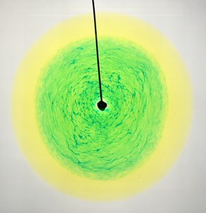
(a) Time series of snapshots from experiment no. 7, showing the xanthan solution (yellow) lubricated by a glucose solution (appears green) that started  $t_L=754$ s later. (b) A snapshot from experiment no. 3, showing (using polar coordinates $(r,{\theta })$) the measured front $r_L({\theta })$ of the lubricating fluid (—–, blue) and $r_N({\theta })$ of the non-Newtonian fluid (—–, purple), and the corresponding fitted circles in (—–, cyan) and (—–, orange), respectively. (c) Evolution of the average (fitted) front radii $r_N$ ( $\triangledown$, yellow) and the corresponding regression STD (- - -, yellow) of experiment no. 3 compared with the theoretical prediction of a non-lubricated GC of a PL fluid (Sayag & Worster Reference Sayag and Worster2013) with identical fluid parameters (– - – -, red). Similarly, for the lubricating fluid front, we show the average front radii $r_L$ ( $\triangledown$, dark green) and STD (- - -, green) compared with predictions for non-lubricated Newtonian GC (Huppert Reference Huppert1982) (– - – -, teal) and lubricated purely Newtonian GC (Kowal & Worster Reference Kowal and Worster2015) with exponent $\beta =0.52$ and coefficient $\xi _L^*=0.27$ (– - – -, dark green). The centres of the fitted circles $O_N,O_L$ ( $+$) remain very close to the centre of the nozzle (shown in more detail in panel d). (d) STDs of the front measurements (- - -) and the centres of the fitted circles $O_N,O_L$ ( $+$) normalised by the instantaneous average fronts $r_N,r_L$.

3. Experimental analysis
We classify the lubricated GC experiments using the four dimensionless numbers
 \begin{align} \mathscr{Q}\equiv \frac{Q_{\ell}}{Q},\quad \mathscr{D}\equiv \frac{\rho_\ell-\rho}{\rho},\quad n,\quad \mathscr{M}\equiv\frac{\mu}{\mu_\ell}=\frac{\rho g}{\mu_\ell} \left(\frac{k}{\rho g}\right)^{{8n}/{(5n+3)}}\left(\frac{t_L^{4}}{Q}\right)^{{(n-1)}/{(5n+3)}}, \end{align}
which represent respectively the sources flux ratio, the reduced density ratio, the PL fluid exponent, and the viscosity ratio. The non-Newtonian fluid viscosity in the latter ratio is based on (2.1) and on the solution of non-lubricated GCs of PL fluids with a small depth-to-radius aspect ratio (Sayag & Worster Reference Sayag and Worster2013). Specifically, the leading-order shear rate in these GCs,  $\dot {\epsilon }=|1/2{\partial } u/{\partial } z|$, where $u$ is the radial velocity and $z$ is the depth coordinate, is scaled with the thickness and radius like $\dot {\epsilon }\sim (\rho g/k)^nH^{2n}/R^n$, where $H$ and $R$ are the depth and radial scales, respectively. These spatial scales have a power-law evolution in time that is determined by a similarity solution (Sayag & Worster Reference Sayag and Worster2013), which we evaluate at the lubricating fluid discharge time $t_L$ to obtain the viscosity scale in (3.1d). In the experiments that we analyse, the lubrication flux was much smaller than the flux of the PL fluid ( $\mathscr {Q}\lesssim 0.06$). The viscosity ratio varied over almost one order of magnitude ( $4700\lesssim \mathscr {M}\lesssim 43\,000$), particularly owing to the wide range of $t_L$ and $Q$ (figure 2c) and owing to the fluid exponent $n>1$, as represented by the last factor in the definition (3.1d) of $\mathscr {M}$. The 1 % and 2 % polymer concentrations led to a small variation in $n$ (figure 1c) and to similar density ratios of $\mathscr {D}_{1\,\%}=0.156$ and $\mathscr {D}_{2\,\%}=0.152$, respectively.
To explore the significance of the interaction between the two fluids, we analyse in the sections that follow the image sequence taken in each experiment to trace the evolution of the two fluid fronts (§ 3.1) and thicknesses (§ 3.2), and we compare the resulting measurements to existing theories of lubricated and non-lubricated flows.
3.1. The front evolution of the lubricating and non-Newtonian fluids
Tracing the position of the fronts of the non-Newtonian fluid  $r_N(t,{\theta })$ and of the lubricating fluid $r_L(t,{\theta })$, where $\theta$ is the angular coordinate, we calculate the average radius of each instantaneous front by fitting a circle (figure 3b). We find that the regression STD can be reduced when using the centres of the fitted circles $O_N$ and $O_L$ as free parameters in addition to the radii (figure 3c,d). This means that the deviation of the front from an axisymmetric shape has two contributions: the centres $O_N, O_L$ that represent translation of the geometric centre of the circular front, and the regression STD of the radii that represent the non-axisymmetric displacement of the fronts with respect to the translated circles. We find that STD $_L, O_L\lesssim 5$ and STD $_N, O_N\lesssim 2$ cm, which implies that the lubricating fluid became more non-axisymmetric and had larger variations in its geometric centre than the non-Newtonian fluid. However, the ratios STD $_i/r_i$ and $O_i/r_i$, where the subscript $i$ represents the two fronts $N \& L$, remain confined (less than $\approx$5 %) and even decay (figure 3d), which implies that the evolution of the fluid fronts remained axisymmetric to the leading order.
To appreciate the resulting evolution of the fronts, we contrast them with existing theories of non-lubricated GCs of PL (Sayag & Worster Reference Sayag and Worster2013) and Newtonian (Huppert Reference Huppert1982) fluids, and lubricated GCs of purely Newtonian fluids (Kowal & Worster Reference Kowal and Worster2015), in which the solutions for the fronts are respectively
 \begin{gather} r_{N}^{\textrm{SW13}}=\xi_{N} b_N t^{({2n+2})/({5n+3})},\quad b_N=\left[{2^{1-n}}Q^{2n+1}\left({\rho g}/{k}\right)^{n}/({n+2})\right]^{1/(5n+3)}, \end{gather}
 \begin{gather}r_{L}^{\textrm{H82}}=\xi_{L} b_L t^{1/2},\quad b_L=\left(Q_\ell^{3}({\rho_\ell-\rho})g/{3\mu_\ell} \right)^{1/8}, \end{gather}
 \begin{gather}r_{L}^{\textrm{KW15}}=\xi_L^*b_L^*t^{\beta},\quad b_L^*=\left(\mathscr{MQ}Q^3{\rho g}/{\mu}\right)^{1/8}= \left(\mathscr{Q}Q^3{\rho g}/{\mu_\ell}\right)^{1/8}, \end{gather}
where for constant flux,  $\xi _N=\xi _L\approx 0.71$ were determined theoretically (Huppert Reference Huppert1982; Sayag & Worster Reference Sayag and Worster2013), and $\xi _L^*\approx 0.27\pm 0.02$, $\beta =0.52\pm 0.02$ were estimated experimentally for the purely Newtonian case in the range $1/\mathscr {M}\ll \mathscr {Q}\ll 1$, which is consistent with the range we consider, though in the late-time limit ( $t/t_L\gg 1$), the exponent $\beta$ is expected to converge to the theoretical value $1/2$ (Kowal & Worster Reference Kowal and Worster2015). We note that these similarity solutions are valid when the thin-film approximation is satisfied, i.e. when $r_i/h_i\gtrsim 10$, where $h_i$ is the characteristic thickness of each fluid layer. We estimate each of these ratios by assuming that the instantaneous fluid volume in each layer is distributed as a disc of radius $r_i$ and thickness $h_i$. Therefore, the thin-film condition becomes $r_N/h={\rm \pi} r_N^3/Qt\gtrsim 10$ for the top fluid, and similarly, $r_L/h_\ell ={\rm \pi} r_L^3/Q_\ell (t-t_L)\gtrsim 10$ for the lubricating fluid.
Results of the comparison to non-lubricated GCs and to purely Newtonian lubricated GCs indicate growing discrepancies between our measured position of the fronts with the existing theories (figure 3c), particularly during the lubricated stage of the flow. Despite the differences, we find that in all the experiments (figure 2c), both fronts follow a power-law time evolution (figure 4). To quantitatively examine the evolution of the fronts, we first consider the front  $r_N$ of the non-Newtonian fluid separately during the non-lubricated interval ( $t/t_L<1$, figure 4a,b), and during the lubricated interval ( $t/t_L\ge 1$, figure 4c). During the initial non-lubricated interval, we expect the front to evolve consistently with (3.2a) as soon as the lubrication-approximation condition is satisfied. Fitting a power-law function of the form (3.2a) for the measured $r_N$ of the 1 % solutions, we find an exponent that corresponds to $n_{1\,\%}=3.2\pm 0.7$ and an intercept that corresponds to $k_{1\,\%}=6.2\pm 0.9$ Pa s $^{1/n}$, which are in close agreement with the independently measured fluid parameters in (2.2). We note that the apparent larger difference in the value of $n_{1\,\%}$ with (2.2) arises from the form of the time exponent $(2n+2)/(5n+3)$, which tends to map small exponent differences to large differences in $n$. More precisely, the exponents corresponding to the rheometer and the GC measurements of the 1 % solutions are respectively $0.424$ and $0.444$, which reflects a very close agreement with the theory (figure 4a). The difference may have originated from the finite equilibration time of the viscosity, as we elaborate in § 4. Similarly, for the 2 % solutions, we find that $n_{2\,\%}=2.1\pm 0.5$ and $k_{2\,\%}=18.1\pm 7.2$ Pa s $^{1/n}$. Here the exponents corresponding to the rheometer and the GC measurements are respectively $0.42$ and $0.46\pm 0.01$, which reflects a larger difference than the 1 % case (figure 4b). Moreover, in this case, the measured $n_{2\,\%}$ is smaller than $n_{1\,\%}$ in contrast with the expected growth of $n$ with concentration that was implied in the rheometer measurement (2.2), which suggests that other effects may be present in addition to finite equilibrium time of the viscosity. Our preliminary experiments (figures 2a and 4a,b) indicate no measurable sensitivity to the substrate wetting conditions or the substrate material (glass or acrylic). Therefore, we propose that wall slip may arise at high polymer concentrations, as we elaborate in § 4.
Evolution of the fluid fronts, measurements and theory. (a,b) Measurements of the front  $r_N(t)$ (markers) during the non-lubricated interval ( $t/t_L<1$) normalised by the flux, for the 1 % (a) and 2 % (b) concentrations. Regression to the experimental measurements ( $\cdots$, black) is compared with the theoretical prediction (3.2a) with the fluid parameters measured by the rheometer in § 2.1 (- - -, grey). (c) The measured front $r_N(t)$ during the lubricated interval ( $t>t_L$), normalised by $r_N(t=t_L)$ and by the inverse of the time exponent in (3.2a) with the fluid exponents measured by the rheometer in § 2.1. The normalised front of a non-lubricated GC (3.2a) is shown (- - -, grey), and is compared with regression to the experimental measurements ( $\cdots$, black). Inset zoomed-in image of the earlier stage that includes the non-lubricated interval. (d) The measured front $r_L(t)$ (markers) normalised with the coefficient $b_L^*$ (3.2c). Regression to the experimental measurements ( $\cdots$, black) is compared with the theoretical prediction (3.2c) of purely Newtonian lubricating GCs (- - -, grey). The markers when the thin-film criterion is first satisfied have black edges. The STD error bars are too small to be presented.

During the lubricated interval ( $t/t_L\ge 1$), we measure a faster propagation of $r_N$ than a non-lubricated GC (figure 4c), which implies a significant impact of lubrication. The response of $r_N$ to the lubrication fluid initialises with a transient acceleration ( $1.5\lesssim t/t_L\lesssim 5$) with respect to the non-lubricated solution, then during $5\lesssim t/t_L$, the front has a power-law evolution with a similar exponent as that predicted for non-lubricated GCs, but with a larger intercept. Specifically, we find that the time exponent based on the GC experiments is $1.01\pm 0.04$ times the theoretical value $(2n+2)/(5n+3)$ of non-lubricated GCs (3.2a), with the fluid exponents $n$ predicted by the rheological measurements (2.2). Therefore, during the developed lubricated stage, the front of the PL fluid $r_N$ propagates faster than that of a corresponding non-lubricated GC, but with the same time exponent within the measurement uncertainty.
The flow of the lubricating fluid was affected by both the normal and shear stresses applied by the surrounding non-Newtonian fluid. Nevertheless, we find that the evolution of  $r_L$ is power law in time with an exponent $0.5\pm 0.02$ (figure 4d), which is identical to, within the measurement uncertainty, the $1/2$ exponent predicted for Newtonian GCs (Huppert Reference Huppert1982; Kowal & Worster Reference Kowal and Worster2015). However, the intercept $b_L^*$ of the purely Newtonian lubricated theory (3.2c) that we use to normalise the experimental data does not lead to a full collapse of the data (figure 4d). Therefore, the intercept in the present case may have a different dependence on the flow parameters and in particular, may depend on the properties of the non-Newtonian fluid. We also note that for all the experiments (figure 2c)
 \begin{equation} b_L/b_L^*=\left(\tfrac{1}{3}\mathscr{D}\mathscr{Q}^2\right)^{1/8}<1, \end{equation}
which implies that the interaction with the top fluid layer in the purely Newtonian case leads to faster propagation of the lower-layer front  $r_L$. This appears to be also the response in the present non-Newtonian case, as can be appreciated in figure 3(c).
3.2. The thickness evolution of the lubricated power-law fluid
Mass conservation implies that the thickness of lubricated GCs should be smaller than that of non-lubricated GCs to account for the former's faster front propagation. To investigate this, we measured the fluid thickness field from the light intensity extracted from the set of images of the propagating GC in the method described below.
When a monochromatic light of intensity  $I_0$ propagates through a fluid layer, the intensity of the transmitted light $I$ drops exponentially with the fluid thickness $h$ according to the Beer–Lambert–Bouguer law (e.g. Bouguer Reference Bouguer1729)
 \begin{equation} h={-}\frac{1}{a_c}\ln(I/I_0), \end{equation}
where  $a_c$ is the attenuation coefficient, which we consider as depth independent. We calculate $a_c$ using the measured normalised intensity $I/I_0$ of a non-lubricated GC together with the known solution for the thickness of a non-lubricated GC of PL fluid
 \begin{equation} h=c_0(Q,\rho,n)t^{(n-1)/(5n+3)}\psi(r/r_N), \end{equation}
where  $c_0$ is a known constant and $\psi$ is the dimensionless solution to a nonlinear differential equation that we solve numerically (Sayag & Worster Reference Sayag and Worster2013). Specifically, we trace the transmitted light intensity along a radius during the non-lubricated phase of the flow, when only the PL fluid is present (figure 5a) to get the evolution of the normalised light intensity along that radius $I(r,t)/I_0$, which consists of red, green and blue (RGB) components defined by the camera's RGB sensor (figure 5b,c). The yellow dye of the PL fluid absorbs mostly the blue range of wavelengths, as defined by the response spectra of the camera's blue-channel sensor, and hardly attenuates the red and green range of wavelengths (see appendix). Therefore, we expect a growing attenuation of the blue component of the normalised intensity with the non-Newtonian fluid thickness (figure 5d). Consequently, fitting the normalised transmission of the blue component of $I(r,t/t_L<1)/I_0$ to (3.4), where (3.5) is substituted for the thickness (figure 6a), we obtain the blue light attenuation coefficient $a_{c={\rm blue}}\approx 0.054\pm 0.0007~$mm $^{-1}$.
Tracing the light intensity transmitted through the evolving flow. (a) Time series (vertical axis) of snapshots in true colour of the rectangular region along a radius (red region, inset), showing the initial non-lubricated phase ( $t/t_L<1$) in which only the non-Newtonian fluid (yellow) is present, and the lubricated phase ( $t/t_L>1$) in which the lubricated fluid (appears green) GC develops as well. (b) The light intensity captured by the camera's blue channel of the image in (a), normalised by the source intensity $I_0$, reveals the thickness distribution of the non-Newtonian fluid at the top layer. (c) The same as in (b) but showing the camera's red channel, which emphasises the distribution of the lubricating fluid. (d) The instantaneous, normalised intensities of the camera's red, green and blue channels along one radius just before the discharge of the lubrication fluid ( $t/t_L=1$, bottom), and some time after ( $t/t_L=3.8$, top).

(a) Computation of the blue-light attenuation coefficient  $a_{c=\mbox {blue}}$ by the regression of selected blue-channel intensity snapshots along a radius during the non-lubricated interval ( $t/t_L<1$) to the known thickness solution (—–, blue) of a non-lubricated GC of PL fluid (Sayag & Worster Reference Sayag and Worster2013). (b) The thickness field of the top fluid layer resolved from the transmitted light intensity, which shows the thickness along a radius at four different times during the non-lubricated phase (i) and during the lubricated phase (ii–iv) (experiment no. 1, —–, orange), compared with the corresponding solution (Sayag & Worster Reference Sayag and Worster2013) for the thickness of a non-lubricated GC of PL fluid (—–, blue). Vertical grid lines mark the measured $r_N$ (- - -, orange) and $r_L$ (- - -, green). (c) A snapshot from an experiment with a higher flux ratio ( $\mathscr {Q}\approx 0.2,\mathscr {M}\approx 7500$), which shows the breaking of axisymmetry and the emergence of radial streams.

Having  $a_{c={\rm blue}}$ also allows us to trace the thickness of the PL fluid where it is over a layer of the lubrication fluid. This can be done even though the light is transmitted through two layers of different fluids because the lubrication fluid is dyed in blue that absorbs mostly in the green–red range and transmits over 96 % of the light intensity in the blue range (see appendix). Therefore, nearly all of the blue-light absorption occurs in the yellow top layer, which implies that we can infer the thickness of the PL fluid throughout the flow using (3.4) with the same coefficient $a_{c={\rm blue}}$.
Results of the conversion of light intensity to thickness (figure 6b) show that during the lubricated phase of the flow ( $t/t_L>1$), the thickness of the top layer dropped over time with respect to that of the corresponding non-lubricated GC of a similar fluid, as we expect, and became nearly uniform along the entire lubricated part (figure 6b ${({ii}\text {--}{iv})}$).
The thickness of the lubricating layer can be resolved from the red component of the transmitted light, which was absorbed mostly by the blue-dyed lubricating fluid and hardly by the yellow-dyed PL fluid (figure 5c,d and appendix). One possible method to convert the intensity measurements to fluid thickness is by using a priori measurements of known fluid thicknesses (e.g. Vernay, Ramos & Ligoure Reference Vernay, Ramos and Ligoure2015). Here we estimate the average thickness of the lubricating film using mass conservation and the known position of the axisymmetric front  $r_L$. Assuming that the lubricating fluid has a uniform thickness $h_\ell$, conservation of mass implies that $h_\ell =Q_\ell (t-t_L)/\rho _\ell {\rm \pi}r_L^2$. Using the parameters of experiment no. 1 (figure 2c) and the measured $r_L(t)$, we find that at $t/t_L=1.2$ ( $r_L=8.05$ cm) $h_\ell \approx 0.437$ mm (figure 6b ${{ii}}$), and at $t/t_L=3.71$ ( $r_L=30.21$ cm) $h_\ell \approx 0.434$ mm (figure 6b ${{iv}}$). This implies that the thickness of the lubricating-fluid layer in the experiment was approximately 25 times thinner than that of the PL fluid layer during most of the flow. Therefore, the thickness profiles of the non-Newtonian fluid in figure 6(b) represent quite accurately the free surface of the GC.
4. Discussion
We assumed that the dominant deformation mechanism of our xanthan solutions in the flow experiments was viscous. To confirm this, we estimate the Debora number  ${\it De}=\lambda /T$, where $\lambda \approx 0.1$ s is the elastic relaxation time for 1 % solutions (Stokes et al. Reference Stokes, Macakova, Chojnicka-Paszun, de Kruif and de Jongh2011) and $T={\rm \pi} r^2 h\rho /Q$ is the characteristic timescale of the flow. Having $h\approx 1$ cm, $Q/\rho \approx 0.5\text {--}5$ cm $^3$ s $^{-1}$, and using $r_N(t_L)\approx 10\text {--}20$ cm for the radius (figure 2c), the smallest timescale we obtain is $T\approx 60$ s, which results in $\textit{De}\approx 0.0017$ at most and implies that elastic deformation is negligible. The radius where elasticity may have been important ( $\textit{De}\approx 1$) is $r\approx 4$ mm, which is the radius of the nozzle. The relaxation time of the 2 % solutions is larger than $\lambda$, but even if it is tenfold larger, $\textit{De}$ will still be low.
The viscous-PL deformation (2.1) that we assume when analysing the GC experiments is based on the viscosity measurements presented in § 2.1. The finite shear-rate dependent, viscosity equilibration time that we observed in these measurements (figure 1c) could potentially imply that the viscosity field in the GC did not have sufficient time to attain the equilibrium value in some regions of the flow. Consequently, the use of (2.1) to represent an instantaneous adjustment of the viscosity to an applied shear rate in the GC may not be strictly valid. However, the good agreement between the theory and experiments in determining the front  $r_N$ during the non-lubricated flow stage (e.g. figure 4a,b and Sayag & Worster Reference Sayag and Worster2013) suggests that the flow was indeed close to quasi-equilibrium, possibly because the strain-rate field in the GC experiments evolved continuously, in contrast with its step-like variation in the viscosity measurements. Consequently, throughout the flow, the instantaneous viscosity field in the GC remained close to the equilibrium values measured in § 2.1 (figure 1c). Nevertheless, the small discrepancy that we measure in the initial non-lubricated stage of the GC flow between the measured front $r_N$ and the theoretical predictions (figure 4a,b) could result from the instantaneous viscosity being further away from equilibrium in some regions of the flow. As the viscosity measurements imply (§ 2.1), the difference between the instantaneous and equilibrium viscosities could peak where the strain rate is smallest. Using the characteristic timescale $T$, we find that the characteristic strain rate in the GC experiments, $T^{-1}$, ranged between $20/{\rm \pi}$ s $^{-1}$ near the nozzle ( $r=0.5$ cm, $Q/\rho =5$ cm $^3$ s $^{-1}$) and $0.0016$ s $^{-1}$ at $r=10$ cm ( $Q/\rho =0.5$ cm $^3$ s $^{-1}$) and $0.0004$ s $^{-1}$ at $r=20$ cm ( $Q/\rho =0.5$ cm $^3$ s $^{-1}$). Therefore, we expect that a discrepancy between the equilibrium viscosity and the instantaneous GC viscosity grows with the radius and inversely with the flux.
Our analysis suggests that the discrepancy between the theoretical predictions (Sayag & Worster Reference Sayag and Worster2013) and the measured front propagation during the non-lubricated interval is larger in the 2 % than in the 1 % concentrations. This discrepancy may be partially explained by the viscosity finite equilibrium time that we discussed previously. Another contribution to this discrepancy may arise from the larger extent of polymer entanglements in the 2 % solution relative to the 1 % solution (the storage modulus of the former is  $\sim 3$ times larger than that of the latter, Martín-Alfonso et al. Reference Martín-Alfonso, Cuadri, Berta and Stading2018). Consequently, one process that could lead to a faster propagation and be more substantial in the 2 % solutions than the 1 % is wall slip at the fluid–solid interface, potentially through adhesive failure of the polymer chains at the solid surface or through cohesive failure owing to disantanglement of chains in the bulk from chains adsorbed at the wall (Brochard & Gennes Reference Brochard and Gennes1992). Such mechanisms would invalidate the theoretically-assumed no-slip condition.
Although we did not calculate the thickness distribution of the lubricating fluid, the true-colour images and the transmitted red-light intensity suggest that it has a complex spatiotemporal structure. In particular, the thickness is non-monotonic, and contains spikes of 50 % reduction in the transmission that appear to propagate downstream with the flow (figure 5c,d). This structure may arise from the roughness of the non-Newtonian fluid free surface, which may imply the presence of a yield stress. Alternatively, an instability of the fluid–fluid interface could lead to the growth of finite-amplitude thickness spikes. Having calculated the thicknesses of the lubricating and PL fluids, we can propose a possible explanation for the observed difference between the sensitivity of the two fluids to the wetting conditions on the substrate, even though both were aqueous solutions. The largest impact of the wetting conditions on the flow was through capillary forces near the fluid front, where the curvature of the interface of the fluid was largest. The significance of this force should be evaluated with respect to the driving gravitational force through the Bond number  $Bo=(\ell /\lambda _c)^2$, where $\ell$ is a characteristic length scale of the flow, and $\lambda _c=\sqrt {\gamma /\rho g}$ is the capillary length of a fluid with density $\rho$ with respect to the air and surface tension coefficient $\gamma$. For both fluids, $\lambda _c\approx 2.5$ mm, because their densities and surface tension coefficients differ by less than 10 %. However, the characteristic scale $\ell$, which most appropriately in this case is represented by the fluid thickness, is equivalent to $h_\ell \approx 0.43$ mm for the lubricating layer and approximately to 10 mm for the polymer solution. Therefore, $Bo\approx 16$ for the non-Newtonian fluid implies negligible capillary forces, whereas $Bo\approx 0.03$ for the Newtonian lubricating fluid implies a more significant role for capillary forces. This could explain why a coating of soap solution had a significant impact on the front of the lubricating fluid and a negligible impact on the front of the non-Newtonian fluid.
The transition to the lubricated interval coincides with the growth of a non-axisymmetric component of the fronts and translation of the GCs geometric centre. However, as the GC evolved, these quantities appeared to become confined and attenuated (figure 3d), which implies that the flow remained axisymmetric to the leading order. This apparent stability may be associated with the substantially lower lubrication flux compared with the flux of the top non-Newtonian fluid. Our hypothesis is reinforced by preliminary experiments with larger  $\mathscr {Q}$, which demonstrate the breakdown of axisymmetry and the development of finger-like patterns in both the lubricating and top fluids (figure 6c). In particular, the non-Newtonian fluid propagated as a stream over each of the apparent fingers in the lubricating fluid, which carried most of the flux, while in the non-lubricated regions located in between the streams, the non-Newtonian fluid was nearly stagnant. Therefore, we expect maximal horizontal shear rates along the margins of the stream and correspondingly minimal viscosity. Such a mechanism, which is absent in the purely Newtonian case (Kowal & Worster Reference Kowal and Worster2019), may be important to sustaining the stream pattern. The formation of these patterns, which are reminiscent to ice streams, will be the subject of our future theoretical and experimental work.
5. Conclusions
Lubricated GCs are controlled by complex interactions between two fluid layers. The lower lubricating layer modifies the friction between the substrate and the top layer, which in turn applies stresses that affect the distribution of the lubricating layer. The resulting flow can vary dramatically from non-lubricated GCs and from purely Newtonian lubricated GCs.
In our experiments at a lower flux ratio ( $\mathscr {Q}<0.06$) than in previous studies, we find that the two fronts follow a power-law evolution with different exponents that are similar to their corresponding non-lubricated GCs. Nevertheless, the fronts propagate faster than those of non-lubricated GCs. Specifically, following a transient acceleration during the initial lubricated stage, the front $r_N$ of the non-Newtonian fluid evolves with the same exponent $(2n+2)/(5n+3)$ as a non-lubricated PL fluid, but with a larger intercept. The larger intercept implies that a lubricated GC of such a non-Newtonian fluid propagates faster than a non-lubricated GC of a similar fluid. Compared with the Newtonian case that has an exponent $1/2$, strain-rate softening fluids ( $n>1$) have a smaller exponent, which implies that, asymptotically in time, the front of a strain-rate softening fluid propagates slower than that of a purely Newtonian lubricated GC and that consequently, the thickness of the non-Newtonian fluid is larger. The front $r_L$ of the lower lubricating fluid evolves with the same exponent $1/2$ as purely Newtonian GCs, but with a larger intercept that appears sensitive to the properties of the overlaying non-Newtonian fluid. Our measurements of the transmitted light intensity allow us to compute the radial distribution of the thickness of the non-Newtonian fluid layer. We find that, in the lubricated region, the thickness is nearly uniform, in contrast with the monotonically declining thickness of non-lubricated GCs (Sayag & Worster Reference Sayag and Worster2013), but consistently with the theoretical prediction for the case of Newtonian lubricated GC (Kowal & Worster Reference Kowal and Worster2015). Similar measurements of the lubricating fluid reveal a nonmonotonic thickness distribution with localised spikes, which is not observed in the case of purely Newtonian lubricated GCs.
Despite these complex thickness distributions, the fronts of the two fluids remain axisymmetric throughout the flow, with a weak non-axisymmetric component that relaxes with time or remaines confined. However, preliminary experiments with  $\mathscr {Q}>0.06$ reveal strong symmetry breaking of the circular fronts and a transition to a stream-like flow, which implies that for a sufficiently large $\mathscr {Q}$, the axisymmetric fronts can become unstable.
The experiments and analyses we present may provide new insights into the rich phenomenology in potentially similar dynamical systems such as ice-sheet systems coupled with hydrological networks. Future research will focus on theoretical analysis of the lubricated flow considered here, by modeling a GC of a PL fluid propagating over a GC of a Newtonian fluid and investigating the resulting axisymmetric flow when the volumes of the two fluids grow in a power law with time. Further research will explore the breaking of circular symmetry and the emergence of radial streams.
Supplementary movies
Supplementary movies are available at https://doi.org/10.1017/jfm.2021.240.
Acknowledgements
We thank D. Bokobza, S. Kabalo and V. Melnichak for their assistance in setting up the experimental apparatus, and to Jungbunzlauer for the xanthan gum.
Funding
This research was supported by the GERMAN–ISRAELI FOUNDATION (grant No. I240430182015).
Declaration of interests
The authors report no conflict of interest.
Appendix. Spectral distribution of the light absorbed by and transmitted through the experimental fluids
We used the light intensity captured by the red–green–blue (RGB) sensor of a Nikon D5500 camera to resolve the thickness of the fluid layers. To measure the spectral distribution of the light source and of the light absorbed by and transmitted through the PL and Newtonian fluids in the flow experiments, we used an AVANTES spectrometer (wavelength range 200–1100 nm). The spectral measurements were performed by positioning the edge of the sensing optical fibre at the same position of the camera that was documenting the flow experiments. Therefore, the light we measured went through the same optical path as in the flow experiments, which included transmission through the glass surface and reflection from the  $45^\circ$ mirror (figure 1a). To measure the spectrum of the fluids, we placed each fluid in a Petri dish and placed it over the glass substrate. The thickness of the non-Newtonian polymer solution (dyed yellow) in one dish was 8 mm and the thickness of the Newtonian glucose solution (dyed blue) in the other dish was 2 mm. The rest of the glass surface was covered with optically opaque fabric, so that only light transmitted through the examined Petri dish reached the spectrometer sensor.
We find that the light sheet that was used as a source in the flow experiments provided a continuous incident spectrum from violet  $\approx$425 nm to red $\approx$700 nm (figure 7a). The blue glucose solution absorbed mostly in the green–red wavelength range (500–700 nm), and the yellow polymer solution absorbed in the blue–violet range ( $\lesssim$500 nm) (figure 7a). To evaluate the spectral response of each of the three channels of the camera's RGB sensor to the light signal, we use the spectral response of a Nikon D5000 camera (Bongiorno et al. Reference Bongiorno, Bryson, Dansereau and Williams2013), which has a similar sensor as the D5500 that we used (figure 7b). The spectral response of the three-channeled RGB sensor to the light transmitted through our yellow PL fluid (figure 7c) is substantial in the blue channel and very weak in the green and red channels, which indicates that the light intensity measured by the blue channel provides a leading-order measurement for the yellow-fluid thickness. Similarly, the spectral response of the camera sensor to the light transmitted through our blue solution (figure 7d) is substantial in the red and green channels and very weak in the blue channel, which indicates that the light intensity measured by the red and green channels provide a leading-order measurement for the blue-fluid thickness. Therefore, light that was transmitted through both fluid layers will have a nearly identical blue-channel spectral distribution as that of a single layer of yellow fluid, which implies that the blue channel provides a measure for the PL fluid thickness throughout the flow.
Spectral distributions of the absorbed and transmitted light through the experimental fluids. (a) The spectral distribution of the light-sheet source (—–, black), and the resulting absorption spectrum of the blue lubricating fluid (—–, gold) and of the yellow polymer fluid (—–, blue). (b) Spectral response of the camera's red, blue and green (RGB) channels (Nikon D5000). (c) Spectral distributions of the source incident light on the camera's RGB sensor  $I_R$ (—–, red), $I_G$ (—–, green) and $I_B$ (—–, blue), compared with the distribution of light transmitted through an 8 mm thick layer of the yellow polymer fluid on the camera's RGB sensor $T_R$ (—–, orange), $T_G$ (—–, light green) and $T_B$ (—–, cyan). (d) Same distribution as in (c), but comparing the light source with the transmitted light through a 2 mm thick layer of the blue lubricating fluid.


 Open access