


1. Introduction
Thermoacoustic instabilities are a major design challenge when developing new gas turbine engines, or when operating existing systems in new regimes and using different fuel compositions. The presence of such instabilities can severely limit the operating range and fuel flexibility of combustion systems, and tools to predict potential thermoacoustic instabilities are essential to obtaining the desired flexibility. A common approach to predicting the thermoacoustic stability of a combustion system is to use acoustic models (Dowling Reference Dowling1997; Dowling & Stow Reference Dowling and Stow2003; Stow & Dowling Reference Stow and Dowling2004; Nicoud et al. Reference Nicoud, Benoit, Sensiau and Poinsot2007; Noiray, Bothien & Schuermans Reference Noiray, Bothien and Schuermans2011; Mensah & Moeck Reference Mensah and Moeck2015; Laera et al. Reference Laera, Schuller, Prieur, Durox, Camporeale and Candel2017a,Reference Laera, Yang, Li and Morgansb), where the nonlinear combustion is accounted for using a flame describing function (FDF) (Dowling Reference Dowling1997). The quality of stability predictions depends on the applicability of the FDF, which is the only link between the combustion process and acoustic mode in such models. There are several approaches to determining the FDF of a system, including simple analytical models (Dowling Reference Dowling1997, Reference Dowling1999; Schuller, Durox & Candel Reference Schuller, Durox and Candel2003; Noiray et al. Reference Noiray, Bothien and Schuermans2011), high fidelity simulations (Krediet et al. Reference Krediet, Beck, Krebs, Schimek, Paschereit and Kok2012; Han & Morgans Reference Han and Morgans2015) and experiments (Kunze, Hirsch & Sattelmayer Reference Kunze, Hirsch and Sattelmayer2004; Balachandran et al. Reference Balachandran, Ayoola, Kaminski, Dowling and Mastorakos2005; Palies et al. Reference Palies, Durox, Schuller and Candel2010; Boudy et al. Reference Boudy, Durox, Schuller, Jomaas and Candel2011; De Rosa et al. Reference De Rosa, Peluso, Quay and Santavicca2016; Nygård & Worth Reference Nygård and Worth2021). A widely used approach in all cases is to study an isolated flame subjected to longitudinal acoustic perturbations.
Real gas turbines, on the other hand, often feature an array of flames, commonly in an annular or a can-annular configuration such as in: Seume et al. (Reference Seume, Vortmeyer, Krause, Hermann, Hantschk, Zangl, Gleis, Vortmeyer and Orthmann1988), Krebs et al. (Reference Krebs, Flohr, Prade and Hoffmann2002), Schuermans, Paschereit & Monkewitz (Reference Schuermans, Paschereit and Monkewitz2006) and Ghirardo et al. (Reference Ghirardo, Gant, Boudy and Bothien2021a). These configurations can also exhibit azimuthal, or transverse, thermoacoustic instabilities as well, as the length scales of the azimuthal and longitudinal dimensions are of a similar order (Poinsot Reference Poinsot2017). Including the potential for significant flame–flame interaction in annular designs, the applicability of a FDF obtained based on a longitudinally excited isolated flame is not necessarily known. There have been some attempts to consider the impact of simultaneous transverse and longitudinal forcing of a single flame in the linear regime (Saurabh, Moeck & Paschereit Reference Saurabh, Moeck and Paschereit2017; Saurabh & Paschereit Reference Saurabh and Paschereit2019), and a modified transfer function accounting for both types of forcing was introduced by O'Connor & Acharya (Reference O'Connor and Acharya2013).
The azimuthal acoustic mode is often a degenerate mode, where the mode can be spinning in either direction, standing or something in between. The mode can be uniquely described by the amplitude  $A$, the nature angle $\chi$, the orientation of the anti-nodal line $n\theta _{0}$ and the temporal phase $\varphi$ when using the recently introduced quaternion expression from Ghirardo & Bothien (Reference Ghirardo and Bothien2018). These four parameters fully define the mode state, and the nature angle describes whether the mode is standing ( $\chi = 0$), spinning in the anti-clockwise (ACW) or clockwise (CW) direction ( $\chi ={\rm \pi} /4$ and $\chi =-{\rm \pi} /4$ respectively) or something in between ( ${\left | \chi \right |} \in {\left (0, {\rm \pi}/4\right )}$). At different locations in the geometry the relation between the azimuthal velocity and the induced axial velocity can differ (Saurabh et al. Reference Saurabh, Moeck and Paschereit2017). Due to a lack of experimental evidence, until very recently, most models assume the heat release rate response of each flame in such a configuration is dependent only on the local pressure, or velocity, fluctuations (Dowling Reference Dowling1997; Dowling & Stow Reference Dowling and Stow2003; Stow & Dowling Reference Stow and Dowling2004; Nicoud et al. Reference Nicoud, Benoit, Sensiau and Poinsot2007; Noiray et al. Reference Noiray, Bothien and Schuermans2011; Wolf et al. Reference Wolf, Staffelbach, Gicquel, Müller and Poinsot2012; Silva et al. Reference Silva, Nicoud, Schuller, Durox and Candel2013; Bauerheim et al. Reference Bauerheim, Parmentier, Salas, Nicoud and Poinsot2014; Mensah & Moeck Reference Mensah and Moeck2015; Laera et al. Reference Laera, Yang, Li and Morgans2017b,Reference Laera, Schuller, Prieur, Durox, Camporeale and Candela; Yang, Laera & Morgans Reference Yang, Laera and Morgans2019). Early signs that this was not necessarily always the case were observed by Nygård et al. (Reference Nygård, Mazur, Dawson and Worth2019), and later shown more explicitly in Nygård, Ghirardo & Worth (Reference Nygård, Ghirardo and Worth2021). In the latter publication, the azimuthal flame describing function (AFDF) was introduced, which is a multiple-input single-output function where the amplitude of each of the two spinning components are the inputs. This dependence of the flame on the two spinning components was conjectured to only be possible due to breaking the mirror symmetry of the system, which happens with co-swirling flames (Nygård et al. Reference Nygård, Ghirardo and Worth2021).
The linear stability of a system can be modelled using a Helmholtz solver for the chosen geometry (Wolf et al. Reference Wolf, Staffelbach, Gicquel, Müller and Poinsot2012; Silva et al. Reference Silva, Nicoud, Schuller, Durox and Candel2013; Bauerheim et al. Reference Bauerheim, Parmentier, Salas, Nicoud and Poinsot2014; Mensah & Moeck Reference Mensah and Moeck2015; Laera et al. Reference Laera, Schuller, Prieur, Durox, Camporeale and Candel2017a; Yang et al. Reference Yang, Laera and Morgans2019), focusing on identifying the mode shapes and frequency of the different modes. One approach to modelling the acoustic modal dynamics in an annular combustor is the Galerkin-based approach, where the flames can be considered point sources (Noiray et al. Reference Noiray, Bothien and Schuermans2011; Ghirardo & Juniper Reference Ghirardo and Juniper2013; Ghirardo & Gant Reference Ghirardo and Gant2019; Faure-Beaulieu & Noiray Reference Faure-Beaulieu and Noiray2020; Ghirardo & Gant Reference Ghirardo and Gant2021). This approach has yielded significant results, such as demonstrating for some conditions the preference for exciting different mode natures, and the observation that noise pushes the mode nature towards standing (Ghirardo & Gant Reference Ghirardo and Gant2019; Faure-Beaulieu & Noiray Reference Faure-Beaulieu and Noiray2020; Ghirardo & Gant Reference Ghirardo and Gant2021). This was all performed assuming the flames only respond to the local pressure. However, in Ghirardo et al. (Reference Ghirardo, Nygård, Cuquel and Worth2021b), the AFDF was used, resulting in a preference for one of the spinning directions, in agreement with experimental results. Recently, Humbert et al. (Reference Humbert, Orchini, Paschereit and Noiray2022b) studied the effect of varying the response of different ‘flames’ by adjusting the gain and time delay in a novel annular configuration with electroacoustic feedback. When the mirror symmetry was preserved, the nature angle distribution was observed to be symmetric. However, as soon as the mirror symmetry was broken by using three unique describing functions for the different flames, a preference for one spinning direction was observed. Humbert et al. (Reference Humbert, Moeck, Paschereit and Orchini2022a) later broke the mirror symmetry by azimuthally offsetting the speakers relative the centre of the injector, mimicking asymmetric, but identical, flames. Again, the mode was observed to prefer one spinning direction, with the preferred side depending on the side of the offset. This supports the symmetry arguments made in Nygård et al. (Reference Nygård, Ghirardo and Worth2021), and warrants the inclusion of such effects in modelling efforts. Using a function with multiple inputs, such as the AFDF, allows asymmetry effects to be included in the system.
In the current paper, the AFDF, which is a multiple-input single-output framework originally constructed using an orthogonal decomposition, is incorporated into the model of Ghirardo & Gant (Reference Ghirardo and Gant2019, Reference Ghirardo and Gant2021) based on the quaternion description of the acoustics. This allows for a direct assessment of the symmetry breaking on the equations describing the evolution of the state space variables, as the degree of asymmetry is shown to be adjustable by a single parameter. With no asymmetry the response is the same as using a conventional FDF, which is compared with a case where the asymmetry is similar to the one observed in Nygård et al. (Reference Nygård, Ghirardo and Worth2021). In this work, the  $A$–
$A$– $2\chi$ plane, where the amplitude $A$ and the nature angle $\chi$ vary, is studied for a range of different gain and noise values, yielding insight into how the solutions depend on different parameter combinations. The model is also used to compare time series simulations with experimental observations of the annular combustor used in Nygård et al. (Reference Nygård, Ghirardo and Worth2021).
2. Model derivation
The model of Ghirardo & Gant (Reference Ghirardo and Gant2021) is based on the following ansatz of the acoustic pressure field (Ghirardo & Bothien Reference Ghirardo and Bothien2018):
 \begin{align} p{\left(\theta, t\right)} = A\cos{\left({n{\left(\theta - \theta_{0}\right)}}\right)}\cos{\left(\chi\right)}\cos{\left({\omega t + \varphi}\right)} + A\sin{\left({n{\left(\theta - \theta_{0}\right)}}\right)}\sin{\left(\chi\right)}\sin{\left({\omega t + \varphi}\right)}. \end{align}
The acoustic mode is determined by four real valued state space variables: the amplitude  $A$; the orientation angle $n\theta _{0}$; the nature angle $\chi$ ( $\chi \in \lbrack -{\rm \pi} /4, {\rm \pi}/4\rbrack$); and the temporal phase $\varphi$. The nature angle quantifies whether the mode is standing ( $\chi = 0$), or spinning in either the ACW ( $\chi = {\rm \pi}/4$) or CW ( $\chi = -{\rm \pi} /4$) direction. All other nature angle values correspond to a mode with both a standing and a spinning component. The expression in (2.1) is equivalent to (Ghirardo & Bothien Reference Ghirardo and Bothien2018)
 \begin{align} 2p{\left(\theta, t\right)} = A\exp({-{\mathrm{i}} n{\left(\theta - \theta_{0}\right)}})\exp({-{\mathrm{k}}\chi})\exp(\kern0.7pt {{\mathrm{j}}{\left(\omega t + \varphi\right)}}) + \operatorname{\text{q.c.}} = \hat{p}\exp(\kern0.7pt {{\mathrm{j}}\omega t}) + \operatorname{\text{q.c.}}, \end{align}
where  ${\mathrm {i}}$, ${\mathrm {j}}$ and ${\mathrm {k}}$ are the three imaginary units of the quaternion numbers, which are not commutative, and $\operatorname {\text {q.c.}}$ is the quaternion conjugate of the preceding term. Then, according to the conventional FDF framework, the heat release rate at position $\theta$ is expressed as
 \begin{equation} 2q{\left(\theta, t\right)} = A\exp({-{\mathrm{i}} n{\left(\theta - \theta_{0}\right)}})\exp({-{\mathrm{k}}\chi})\exp(\kern0.7pt {{\mathrm{j}}{\left(\omega t + \varphi\right)}}) {\hat{Q}_{\theta,{conv}}} + \operatorname{\text{q.c.}}, \end{equation}
where the conventional FDF  ${\hat {Q}_{\theta,{conv}}}$ can have a real and a ${\mathrm {j}}$-imaginary component in general. This simply states that the heat release rate is proportional to the local pressure fluctuations with a potential phase response due to the ${\mathrm {j}}$-component.
Ghirardo & Gant (Reference Ghirardo and Gant2021) showed that the fluctuating mass and momentum conservation equations yield the following governing equation for the state space variables when expressing the pressure and heat release rate through the above expressions:
 \begin{align} &{\left(\ln
A\right)}^{\prime} + {\left(n\theta_{0}^{\prime} +
\varphi^{\prime}\sin{\left(2\chi\right)}\right)}{\mathrm{i}}
+ \varphi^{\prime}\cos{\left(2\chi\right)}{\mathrm{j}} -
\chi^{\prime}{\mathrm{k}} \nonumber\\ &\quad =
{\left(-\frac{\omega}{2} +
\frac{\omega_{0}^{2}}{2\omega}\right)}\exp({-{\mathrm{k}}\chi}){\mathrm{j}}\exp({{\mathrm{k}}\chi})
+ \frac{\sigma}{\sqrt{2}A}\mu_{z}\nonumber\\ &\qquad +
\frac{1}{2}\frac{1}{2{\rm \pi}}\int_{0}^{2{\rm \pi}}
\left(\exp({2{\mathrm{i}}{n{\left(\theta -
\theta_{0}\right)}}})\exp({{\mathrm{k}}\chi}) +
\exp({-{\mathrm{k}}\chi})\right)
{\hat{Q}_{\theta,{conv}}}{\left(A, \chi, \theta,
\theta_{0}\right)}
\mathrm{d}\theta\exp({{\mathrm{k}}\chi})\nonumber\\ &\qquad
+ \frac{\sigma^{2}}{4A^{2}}{\left(1 +
\tan{\left(2\chi\right)}{\mathrm{k}}\right)},
\end{align}
\begin{align} &{\left(\ln
A\right)}^{\prime} + {\left(n\theta_{0}^{\prime} +
\varphi^{\prime}\sin{\left(2\chi\right)}\right)}{\mathrm{i}}
+ \varphi^{\prime}\cos{\left(2\chi\right)}{\mathrm{j}} -
\chi^{\prime}{\mathrm{k}} \nonumber\\ &\quad =
{\left(-\frac{\omega}{2} +
\frac{\omega_{0}^{2}}{2\omega}\right)}\exp({-{\mathrm{k}}\chi}){\mathrm{j}}\exp({{\mathrm{k}}\chi})
+ \frac{\sigma}{\sqrt{2}A}\mu_{z}\nonumber\\ &\qquad +
\frac{1}{2}\frac{1}{2{\rm \pi}}\int_{0}^{2{\rm \pi}}
\left(\exp({2{\mathrm{i}}{n{\left(\theta -
\theta_{0}\right)}}})\exp({{\mathrm{k}}\chi}) +
\exp({-{\mathrm{k}}\chi})\right)
{\hat{Q}_{\theta,{conv}}}{\left(A, \chi, \theta,
\theta_{0}\right)}
\mathrm{d}\theta\exp({{\mathrm{k}}\chi})\nonumber\\ &\qquad
+ \frac{\sigma^{2}}{4A^{2}}{\left(1 +
\tan{\left(2\chi\right)}{\mathrm{k}}\right)},
\end{align}
where primes denote time derivatives. Up to this point, the equation holds for arbitrary describing functions, and  ${\hat {Q}_{\theta,{conv}}}$ will be discussed in the next section. The left-hand side contains all the time derivatives of the state space variables $A$,
$A$,  $n\theta _{0}$, $\varphi$ and $\chi$, which are assumed to change much slower than the fast oscillations at frequency $f = \omega / 2{\rm \pi}$. A comprehensive explanation of the terms is presented in Ghirardo & Gant (Reference Ghirardo and Gant2021), but a brief summary is recalled in the following. The first term on the right-hand side is a frequency shift term between the oscillation frequency $\omega$ and the azimuthal frequency $\omega _{0}$ determined by the geometry and operating conditions, which can influence the orientation $n\theta _{0}$ and the temporal phase $\varphi$. The integral term describes the effect of the heat release rate, and contains the describing function ${\hat {Q}_{\theta,{conv}}}$. The two remaining terms are related to the stochastic white background noise of intensity $\sigma$. The last term is the deterministic effect of the noise and the term on the first line of the equation is proportional to the stochastic variable $\mu _{z}$. An important implication of the $\tan {\left (2\chi \right )}$ term is that the fixed points of the system are pushed away from the purely spinning solutions in the presence of noise ( $\sigma > 0$) (Ghirardo & Gant Reference Ghirardo and Gant2021).
2.1. Flame model
In the original formulation, (2.4), the describing function  ${\hat {Q}_{\theta,{conv}}}$ has a nature angle dependence in general, but there was not any evidence to suggest the exact form of this dependence. The first discussion of a nature angle dependence was presented in Ghirardo et al. (Reference Ghirardo, Nygård, Cuquel and Worth2021b), based on experimental evidence suggesting the heat release rate response to the two spinning directions in an annular combustor with co-swirling flames is different. However, due to the very limited experimental evidence at the time, the functional form of the nature angle was based on an educated guess. This changed with the introduction of the AFDF in Nygård et al. (Reference Nygård, Ghirardo and Worth2021), which is based on more experimental evidence. In the AFDF framework, the heat release rate response is modelled as two components, each linked to the corresponding spinning component of the acoustic mode through a separate gain and phase in general, as observed to be the case in Nygård et al. (Reference Nygård, Ghirardo and Worth2021). An important implication of this is that the nature angles of the acoustic mode and the heat release rate mode are not necessarily the same, which requires a specialisation of the entire integral term in (2.4) when replacing the conventional describing function.
Starting with the pressure distribution, the AFDF framework was developed using an orthogonal description with two counter-propagating wave components
 \begin{align} 2p{\left(\theta, t\right)} = \frac{1}{\sqrt{2}}{\lbrack A_{-}\exp({-{\mathrm{i}}{n{\left(\theta - \theta_{0}\right)}}}) + A_+ \exp({{\mathrm{i}}{n{\left(\theta - \theta_{0}\right)}}})\rbrack}\exp({{\mathrm{i}}{\left({\omega t + \varphi}\right)}}) + \operatorname{\text{c.c.}}, \end{align}
where  ${\mathrm {i}}$ is the imaginary unit of complex numbers. The amplitudes $A_{\pm }$, describing the magnitude of the ACW ( $-$) and CW ( $+$) spinning components, are chosen to be real valued, and $\operatorname {\text {c.c.}}$ is the complex conjugate of the previous term. The normalisation factor $1/\sqrt {2}$ is chosen such that, in the case of a spinning mode $\chi =\pm {\rm \pi}/4$, the amplitude $A$ in (2.1) is $A = A_{\mp }$ with $A_{\pm } = 0$. The state space parameters $n\theta _{0}$ and $\varphi$ are shared between (2.1) and (2.5), and the amplitude $A$ and nature angle $\chi$ are related to the amplitudes $A_{\pm }$ through (Ghirardo & Bothien Reference Ghirardo and Bothien2018)
 \begin{gather} A_{-} = \frac{A}{\sqrt{2}}{\left(\cos\chi + \sin\chi\right)}, \end{gather}
 \begin{gather}A_+{=} \frac{A}{\sqrt{2}}{\left(\cos\chi - \sin\chi\right)}. \end{gather}
 Assuming the annular geometry has  $M$ acoustically compact flames in the azimuthal direction $\theta$, which can be treated as point sources, the total heat release rate can be expressed as
 \begin{equation} q{\left(\theta, t\right)} = 2{\rm \pi}\sum_{m=0}^{M-1}q_{m}{\left(t\right)}\delta{\left(\theta - \theta_{m}\right)}, \end{equation}
where  $q_{m}$ is the heat release rate response of flame $m$ located at $\theta _{m} = 2{\rm \pi} m/M$ and $\delta$ is the Dirac delta distribution. When the response is approximately in the linear regime, $q_{m}$ is given by a similar expression to (2.5) (Nygård et al. Reference Nygård, Ghirardo and Worth2021)
 \begin{align} 2q_{m}{\left(t\right)} = \frac{1}{\sqrt{2}}{\lbrack \hat{q}_{-}\exp({-{\mathrm{i}}{n{\left(\theta_{m} - \theta_{0}\right)}}}) + \hat{q}_+\exp({{\mathrm{i}}{n{\left(\theta_{m} - \theta_{0}\right)}}})\rbrack} \exp({{\mathrm{i}}{\left(\omega t + \varphi\right)}}) + \operatorname{\text{c.c.}}, \end{align}
where  $\hat {q}_{\pm } = q_{\pm }\exp ({{\mathrm {i}}\phi _{\pm }})$ are the complex valued amplitudes of two counter-spinning components of heat release rate oscillations at frequency $\omega$ and azimuthal order $n$. The magnitude $q_{\pm }$ describes the amplitude and $\phi _{\pm }$ is the phase relative to the corresponding pressure mode component in (2.5). The AFDF links the spinning heat release rate component amplitudes $\hat {q}_{\pm }$ to the corresponding acoustic mode component through (Nygård et al. Reference Nygård, Ghirardo and Worth2021)
 \begin{equation} {\text{FDF}^{{\pm}}}{\left(\hat{u}_{{\pm}}\right)} = \frac{\hat{q}_{{\pm}}{\left({\left| \hat{u}_{{\pm}}\right|}\right)} / \bar{Q}}{\hat{u}_{{\pm}} / U_{bulk}}, \end{equation}
where  $\bar {Q}$ is the mean heat release rate and $U_{bulk}$ is the axial bulk velocity. There is no explicit frequency dependence in the above expression as the annular geometry determines the acoustic wavelength of the azimuthal pressure mode, which fixes the frequency for a given operating condition. The acoustic mode components are quantified through the azimuthal axial velocity components $\hat {u}_{\pm }$, which are the axial velocities in the burners induced by the azimuthal acoustic field in the combustion chamber. However, it can be shown that the AFDF in (2.9) can be described in terms of the acoustic pressure amplitudes $A_{\pm }$ instead, with a constant complex valued scaling factor $\hat {C}$, which is system specific (the axial velocities in the injectors can be calculated by multiplying the local acoustic pressure value by the admittance of the whole upstream system for azimuthal forcing separately for each spinning component and then summed), separating the two definitions
 \begin{equation} {\text{FDF}^{{\pm}}}{\left(A_{{\pm}}\right)} = \hat{C}{Q^{{\pm}}}{\left(A_{{\pm}}\right)}\exp({{\mathrm{i}}\phi_{{\pm}}{\left(A_{{\pm}}\right)}}) = \hat{C}\frac{\hat{q}_{{\pm}}{\left(A_{{\pm}}\right)}}{A_{{\pm}}}. \end{equation}
Here,  ${Q^{\pm }}$ is a real valued gain, and $\phi _{\pm }$ is the real valued phase between the azimuthal heat release rate component with complex valued amplitude $\hat {q}_{\pm }$ and the corresponding azimuthal pressure component. Figure 1 presents the data obtained in Nygård et al. (Reference Nygård, Ghirardo and Worth2021) using the alternative description in (2.10).
Azimuthal flame describing function expressed in terms of pressure component amplitudes based on the data in Nygård et al. (Reference Nygård, Ghirardo and Worth2021). The heat release rate fluctuation amplitude  $\hat {q}_{\pm }$ is normalised by the temporal mean heat release rate. The ACW ${\left ({\left | \hat {q}_{-}\right |}\right )}$ component of the AFDF is observed to have a higher heat release rate amplitude than the CW ${\left ({\left | \hat {q}_+\right |}\right )}$ component for a given amplitude $A_{\pm }$.

Using (2.10) to insert for  $\hat {q}_{\pm }$ in (2.8) yields the following expression for $q_{m}$:
 \begin{align} 2q_{m}{\left(t\right)} &=
\frac{1}{\sqrt{2}}{\lbrack A_+{Q^+}{(A_+)}
\exp({{\mathrm{i}}{n{(\theta_{m} - \theta_{0, q})}}}) +
A_{-}{Q^{-}}{(A_{-})}\exp({-{\mathrm{i}}{n{(\theta_{m} - \theta_{0, q})}}})\rbrack}\nonumber\\
&\quad \times \exp({{\mathrm{i}}{(\omega t +
\varphi_{q})}}) + \operatorname{\text{c.c.}},\end{align}
\begin{align} 2q_{m}{\left(t\right)} &=
\frac{1}{\sqrt{2}}{\lbrack A_+{Q^+}{(A_+)}
\exp({{\mathrm{i}}{n{(\theta_{m} - \theta_{0, q})}}}) +
A_{-}{Q^{-}}{(A_{-})}\exp({-{\mathrm{i}}{n{(\theta_{m} - \theta_{0, q})}}})\rbrack}\nonumber\\
&\quad \times \exp({{\mathrm{i}}{(\omega t +
\varphi_{q})}}) + \operatorname{\text{c.c.}},\end{align}
where all the variables are real valued and the following definitions have been introduced:
 $$\begin{gather} n\theta_{0, q} = n\theta_{0, q}{\left(A_+, A_{-}\right)} = n\theta_{0} + {\Delta\phi_{q}}{\left(A_+, A_{-}\right)}, \end{gather}$$
 $$\begin{gather}\varphi_{q} = \varphi_{q}{\left(A_+, A_{-}\right)} = \varphi + \bar{\phi}_{q}{\left(A_+, A_{-}\right)}, \end{gather}$$
 $$\begin{gather}2{\Delta\phi_{q}} = 2{\Delta\phi_{q}}{\left(A_+, A_{-}\right)} = \phi_+{\left(A_+\right)} - \phi_{-}{\left(A_{-}\right)}, \end{gather}$$
 $$\begin{gather}2\bar{\phi}_{q} = 2\bar{\phi}_{q}{\left(A_+, A_{-}\right)} = \phi_+{\left(A_+\right)} + \phi_{-}{\left(A_{-}\right)}. \end{gather}$$
Since (2.11) is of the same form as the pressure distribution in (2.5), the heat release rate mode can also be expressed as
 \begin{align} q_{m}{(t)} &=
A{Q}{(A, \chi)}\lbrack
\cos{({n{(\theta_{m} - \theta_{0,
q})}})}\cos{(\chi_{q})}\cos{(\omega
t + \varphi_{q})}\nonumber\\ &\quad
+\sin{({n{(\theta_{m} - \theta_{0,
q})}})}\sin{(\chi_{q})}\sin{(\omega
t + \varphi_{q})}\rbrack,
\end{align}
\begin{align} q_{m}{(t)} &=
A{Q}{(A, \chi)}\lbrack
\cos{({n{(\theta_{m} - \theta_{0,
q})}})}\cos{(\chi_{q})}\cos{(\omega
t + \varphi_{q})}\nonumber\\ &\quad
+\sin{({n{(\theta_{m} - \theta_{0,
q})}})}\sin{(\chi_{q})}\sin{(\omega
t + \varphi_{q})}\rbrack,
\end{align}
where  ${Q}$ is the describing function of flame $m$ in the quaternion framework. Relating the orthogonal (2.11) and the quaternion ansatz (2.13), similar to (2.6), the following expressions for ${Q}$ and $\chi _{q}$ are obtained:
 \begin{gather} {Q}{\left(A, \chi\right)} = {Q^{st}} \sqrt{1 + \frac{R^{2} - 1}{R^{2} + 1}\sin{\left(2\chi\right)}}, \end{gather}
 \begin{gather}\chi_{q}{\left(A, \chi\right)} = \arctan{\left(\frac{{\left(R - 1\right)}\cos\chi + {\left(R + 1\right)}\sin\chi}{{\left(R + 1\right)}\cos\chi + {\left(R - 1\right)}\sin\chi}\right)}, \end{gather}
where the following shorthand notations were introduced:
 \begin{gather} {Q^{st}}{(A, \chi)} = \sqrt{\tfrac{1}{2}{({\lbrack {Q^{-}}{left(A, \chi)}\rbrack}^{2} + {\lbrack {Q^+}{(A, \chi)}\rbrack}^{2})}}, \end{gather}
 \begin{gather}R{\left(A, \chi\right)} = \frac{{Q^{-}}{\left(A, \chi\right)}}{{Q^+}{\left(A, \chi\right)}}. \end{gather}
It is observed that, for a standing mode  $\chi = 0$, (2.14a) yields ${Q} = {Q^{st}}$. Hence, ${Q^{st}}$ is the heat release rate gain to a standing acoustic pressure mode. The parameter $R$ is the ratio between the slopes in figure 1, which corresponds to the gain ratio between the ACW component and the CW component of the AFDF. For non-swirling flames, the flames are expected to have the same response to the ACW and CW components ( $R = 1$) due to the mirror symmetry (Nygård et al. Reference Nygård, Ghirardo and Worth2021), simplifying the equations back to the conventional case where ${Q}{\left (A, \chi \right )} = {Q^{st}}$ and $\chi _{q} = \chi$. The expressions in (2.14) are equivalent to corresponding conventional FDF expressions when $R = 1$, as the describing function amplitude becomes independent of the nature angle and the heat release rate nature angle is equal to the acoustic nature angle.
2.1.1. Nonlinear flame saturation with two inputs
Thermoacoustic instabilities are bounded in amplitude, most often because the heat release rate response diminishes at large amplitudes (Dowling Reference Dowling1997). Usually, this is accounted for by introducing a saturation on the gain  ${\hat {Q}_{\theta,{conv}}}$ in (2.3) as a function of amplitude $A$. Expressing the heat release rate of a single flame in the linear regime as
 \begin{equation} \frac{\hat{q}}{\bar{Q}} = {\text{FTF}}\frac{\hat{p}}{\bar{p}}, \end{equation}
the nonlinear equivalent is often expressed as
 \begin{equation} \frac{\hat{q}}{\bar{Q}} = F{\left({\left| \frac{\hat{p}}{\bar{p}}\right|}\right)}\exp\left({{\mathrm{i}}\Delta\varphi{\left({\left| \frac{\hat{p}}{\bar{p}}\right|}\right)}}\right){\text{FTF}}\frac{\hat{p}}{\bar{p}}, \end{equation}
where  $\bar {Q}$ is the mean heat release rate and $\bar {p}$ is the mean pressure. In (2.17), the nonlinear saturation depends on the local amplitude of acoustic pressure. The gain of the transfer function is modified by the inclusion of $F$, and an amplitude-dependent phase is introduced through the $\Delta \varphi$ term. The following constraints ensure (2.17) is equivalent to (2.16) in the low amplitude limit:
 \begin{equation} \lim_{{\left| {\hat{p}}/{\bar{p}}\right|}\rightarrow 0} F{\left({\left| \frac{\hat{p}}{\bar{p}}\right|}\right)} = 1, \quad \lim_{{\left| {\hat{p}}/{\bar{p}}\right|}\rightarrow 0} \Delta\varphi{\left({\left| \frac{\hat{p}}{\bar{p}}\right|}\right)} = 0. \end{equation}
Applying the same principle to the AFDF, which has two inputs, will not work as the heat release rate fluctuations at the pressure node are not necessarily zero, as illustrated by data obtained from Nygård et al. (Reference Nygård, Ghirardo and Worth2021) in figure 2(a). Therefore, the heat release rate response would never saturate at the pressure node, it would instead scale linearly with the amplitude  $A$ of the acoustic mode, as shown in figure 2(b).
(a) The normalised heat release rate mode envelope for an approximately standing mode shows the local heat release rate amplitudes are non-zero at pressure nodes. The resulting heat release rate envelope after applying a conventional saturation model, which is based on the local pressure or local acoustic velocity amplitude, for increasing acoustic amplitudes A is shown in (b). As A increases, the output keeps increasing at the nodes because the acoustic pressure is identically zero at that location. The grey shaded area represents the shape of the acoustic pressure mode envelope.

To ensure that all the flames saturate, the nonlinear saturation is proposed to depend on the local heat release rate amplitude  $A_{q}$. The saturation of (2.14a) becomes
 \begin{equation} {Q}{\left(A_{q}\right)} = {\left({Q^{st}}\sqrt{1 + \frac{R^{2}-1}{R^{2}+1}\sin{\left(2\chi\right)}}\right)}F{\left(A_{q}\right)}, \end{equation}
and the phase difference  $\Delta \varphi$ from (2.17) is included by allowing a mode dependence for $\bar {\phi }_{q}$ and ${\Delta \phi _{q}}$ in (2.12). The local linear heat release rate amplitude is defined as
 \begin{align}
\frac{A_{q}{\left(\theta\right)}}{A} &= \sqrt{1 +
\frac{R^{2}-1}{R^{2}+1}\sin{\left(2\chi\right)}}\nonumber\\
&\quad\times \sqrt{\cos^{2}{\lbrack
{n{(\theta - \theta_{0, q})}}\rbrack}\cos^{2}{(\chi_{q})} +
\sin^{2}{\lbrack {n{(\theta - \theta_{0, q})}}\rbrack}\sin^{2}{(\chi_{q})}}, \end{align}
\begin{align}
\frac{A_{q}{\left(\theta\right)}}{A} &= \sqrt{1 +
\frac{R^{2}-1}{R^{2}+1}\sin{\left(2\chi\right)}}\nonumber\\
&\quad\times \sqrt{\cos^{2}{\lbrack
{n{(\theta - \theta_{0, q})}}\rbrack}\cos^{2}{(\chi_{q})} +
\sin^{2}{\lbrack {n{(\theta - \theta_{0, q})}}\rbrack}\sin^{2}{(\chi_{q})}}, \end{align}
which is the fluctuation amplitude of the heat release rate expression in (2.13) normalised by  ${Q^{st}}$. This choice ensures that even the flames in the pressure node saturate to a finite level, as illustrated in figure 3(b). The structure of (2.19) limits the applicability to flames whose gain does not increase as a function of the forcing amplitude, which is the most typical case. The functional form of the saturation function $F$ is chosen to be (Ghirardo et al. Reference Ghirardo, Gant, Boudy and Bothien2021a)
 \begin{equation} F{\left(A_{q}\right)} = \frac{2}{1 + \sqrt{1 + {\lbrack \kappa A_{q}{(A, \chi, \theta, \theta_{0})}\rbrack}^{2}}}, \end{equation}
where  $\kappa$ is a nonlinear saturation constant. The form in (2.21) will only be used in the numerical results, and the theoretical results in § 2.2 are independent of the functional form of $F$. The monotonically non-decreasing function in (2.21) is chosen as it yields a smooth saturation of the heat release rate approaching a constant level at high amplitudes, as illustrated in figure 3(a). Other functions, such as the one used by Dowling (Reference Dowling1997) or the cubic polynomial used by Noiray et al. (Reference Noiray, Bothien and Schuermans2011), can also be considered, but they do not have a smooth saturation or a finite heat release rate amplitude as the pressure amplitude approaches infinity, respectively.
Normalised heat release rate for a single flame (a) and for all flames subjected to a standing acoustic mode (grey shaded area) according to (2.19) and (b) using the saturation function  $F$ in (2.21). The heat release rates saturate smoothly, approaching the same finite limit. Using the local heat release rate amplitude $A_{q}$ is shown to saturate the response for all flames, even when located at a pressure node.

The actual experimental quantitative validation of a specific saturation function among the ones discussed above would require experimental data from a forced experiment in a higher amplitude range than the current experimental set-up allows. However, this does not diminish the conclusions in this section. A sensitivity analysis of the exact expression used in (2.21) was performed (Appendix C in supplementary material available at https://doi.org/10.1017/jfm.2023.921), comparing it with saturation functions used by Dowling (Reference Dowling1997), Noiray et al. (Reference Noiray, Bothien and Schuermans2011) and Ghirardo et al. (Reference Ghirardo, Nygård, Cuquel and Worth2021b). The other saturation functions were found to yield qualitatively the same results as discussed later in this work.
2.1.2. Alternative nonlinear saturation with two inputs
The AFDF also allows  ${Q^{\pm }}$ to depend on the corresponding spinning acoustic mode amplitudes $A_{\pm }$. It could therefore be reasonable to assume, instead of (2.19), that ${Q^+}$ and ${Q^{-}}$ would approach zero as $A_+$ and $A_{-}$ grow sufficiently large, respectively. For example, it could be assumed that each component is inversely proportional to the corresponding acoustic amplitude in the high amplitude limit
 \begin{equation} {Q^{{\pm}}}{\left(A_{{\pm}}\right)} \propto \frac{1}{A_{{\pm}}}. \end{equation}
However, assuming this is the only saturation mechanism leads to several unphysical effects. For example, the heat release rate of all the burners would saturate by the same percentage independent of being located at a node or an anti-node, which is not physical. Another unphysical feature of the assumption in (2.22) is that the heat release rate nature angle  $\chi _{q}$ becomes independent of the acoustic nature angle $\chi$, except for perfectly spinning modes ${\left | \chi \right |} = {\rm \pi}/4$. The expression for $\chi _{q}$ in this limit in the open interval ${\left (-{\rm \pi} /4, {\rm \pi}/4\right )}$ is
 \begin{equation} \lim_{\substack{A\rightarrow\infty\\ {\left| \chi\right|} < {\rm \pi}/4}} \chi_{q} = \arctan{\left(\frac{R_{0} - 1}{R_{0} + 1}\right)}, \end{equation}
where  $R_{0}$ is the value of $R$ in the low amplitude limit. Combined with the apparent linearity of the heat release rate components in figure 1, the ratio $R = {Q^{-}} / {Q^+}$ of AFDF components is assumed to be independent of the individual acoustic amplitudes $A_{\pm }$ in this work.
2.2. The effect of the AFDF on the governing equation
To implement the AFDF in the model of Ghirardo & Gant (Reference Ghirardo and Gant2021), the first step is to replace (2.3) by
 \begin{equation} 2q{(\theta,
t)} = A\exp({-{\mathrm{i}} {n{(\theta -
\theta_{0, q})}}})\exp({-{\mathrm{k}}\chi_{q}})\exp
(\kern0.7pt {{\mathrm{j}}{(\omega t + \varphi_{q})}}) {Q_{\theta}} +
\operatorname{\text{q.c.}},
\end{equation}
\begin{equation} 2q{(\theta,
t)} = A\exp({-{\mathrm{i}} {n{(\theta -
\theta_{0, q})}}})\exp({-{\mathrm{k}}\chi_{q}})\exp
(\kern0.7pt {{\mathrm{j}}{(\omega t + \varphi_{q})}}) {Q_{\theta}} +
\operatorname{\text{q.c.}},
\end{equation}
where the following shorthand notation is introduced:
 \begin{equation} {Q_{\theta}} = 2{\rm \pi}\sum_{m=0}^{M-1}{Q}\delta{\left(\theta - \theta_{m}\right)}. \end{equation}
This is equivalent to (2.7) after inserting the expression for  $q_{m}$ in (2.13). Additionally, the lump parameter $M\alpha$ describing the acoustic damping of the system included in ${\hat {Q}_{\theta,{conv}}}$ in (2.4) (Ghirardo & Gant Reference Ghirardo and Gant2021) is extracted from the describing function. It is then possible to show (Appendix A) that the governing equation from (2.4) becomes

independent of the functional form of the saturation function  $F$ in (2.19). The main modifications to (2.4) are the use of the AFDF for the describing function expression ${Q_{\theta }}$, and the state space parameters $n\theta _{0}$ and $\chi$ have become $n\theta _{0,q}$ and $\chi _{q}$ inside the integral term (highlighted in blue). Additionally, there are two extra terms due to the phase difference and mean phase of the two components of the AFDF (highlighted in red) that were introduced in (2.12c) and (2.12d).
2.2.1. Fourier series representation of heat release rate source term
To get a better understanding of the effect of the new terms in (2.26), it is convenient to express the heat release rate of each flame in terms of a Fourier series (Ghirardo et al. Reference Ghirardo, Gant, Boudy and Bothien2021a)
 \begin{equation} {Q} =
\sum_{r=0}^{M/2}N^{{(r)}}\cos{(r{\lbrack \theta_{m} - \theta^{{(r)}} - \theta_{0,
q}\rbrack})}, \end{equation}
\begin{equation} {Q} =
\sum_{r=0}^{M/2}N^{{(r)}}\cos{(r{\lbrack \theta_{m} - \theta^{{(r)}} - \theta_{0,
q}\rbrack})}, \end{equation}
where the Fourier series coefficients  $N^{{\left (r\right )}}$ are defined as
 \begin{gather} N^{{\left(r\right)}} = {(2 - \delta_{r,0} - \delta_{r,M/2})}\frac{1}{M}\sum_{m=0}^{M-1}\cos{(r{\lbrack \theta_{m} - \theta^{{(r)}} - \theta_{0, q}\rbrack})}{Q}, \end{gather}
 \begin{gather}0 = {(2 - \delta_{r,0} - \delta_{r,M/2})}\frac{1}{M}\sum_{m=0}^{M-1}\sin{(r{\lbrack \theta_{m} - \theta^{{(r)}} - \theta_{0, q}\rbrack})}{Q}. \end{gather}
Note the use of  $\theta _{0, q} = \theta _{0} + {\Delta \phi _{q}}$ in this definition, compared with the $\theta _{0}$ used in the definition by Ghirardo et al. (Reference Ghirardo, Gant, Boudy and Bothien2021a). Following the derivation of Ghirardo et al. (Reference Ghirardo, Gant, Boudy and Bothien2021a), it can be shown that twice the heat release rate integral can be expressed as

where we observe that not all  $N^{(r)}$ $r = 0, 1, \ldots, M/2$ play a role, but just $N^{(0)}$ and $N^{(2n)}$. As expected, this is the same expression as the one in Ghirardo et al. (Reference Ghirardo, Gant, Boudy and Bothien2021a, (A11)) when $\chi = \chi _{q}$ and $\bar {\phi }_{q} = {\Delta \phi _{q}} = 0$ except for the $M\alpha$ term, which is included separately in (2.26) here.
To highlight the effect of the above modification to the heat release rate integral, the quaternion valued equation in (2.26) can be expressed as four real valued equations. Figure 1 suggests that the phase difference  ${\Delta \phi _{q}}$ between the two components is relatively low at realistic amplitudes for self-excited thermoacoustic instabilities. The same applies for the mean phase $\bar {\phi }_{q}$, and therefore ${\Delta \phi _{q}}$ and $\bar {\phi }_{q}$ are set to zero to simplify the discussion of the main effect of the nature angle difference $\Delta \chi = \chi _{q} - \chi$. Inserting for the assumptions yields the following four real valued equations:


with the assumption of  $\omega = \omega _{0}$ for simplicity and $\mu _{0,1,2,3}$ are the individual stochastic components of $\mu _{z}$ in (2.26). The black terms are the same as the ones originally derived by Ghirardo & Gant (Reference Ghirardo and Gant2021) and Ghirardo et al. (Reference Ghirardo, Gant, Boudy and Bothien2021a), and the coloured terms are the new additions and modifications. In the original equation given by (2.4), the zeroth Fourier component $N^{{\left (0\right )}}$ was only present in the time derivative of the amplitude. However, in (2.30) the term has been redistributed to also be a source term for the nature angle of the acoustic mode in (
). This redistribution is achieved through the introduction of  $\cos {\left (\Delta \chi \right )}$ in (
) and the  $\sin {\left (\Delta \chi \right )}$ term in (
), making the degree of redistribution dependent on the acoustic mode through (2.14b). Additionally, the nature angle difference  $\Delta \chi$ slightly modifies how the $2n$ Fourier coefficient is distributed as a source term through the addition of $\Delta \chi$ in $\sin {\left (2\chi + \Delta \chi \right )}$ and $\cos {\left (2\chi + \Delta \chi \right )}$. As expected, the original equations, as presented in Ghirardo et al. (Reference Ghirardo, Gant, Boudy and Bothien2021a), are retrieved for $\Delta \chi = 0$.
While the mean phase  $\bar {\phi }_{q}$ and phase difference ${\Delta \phi _{q}}$ were assumed to be zero for simplicity, the main effect of including a non-zero value is a further redistribution of the Fourier components to all the equations, as shown in Appendix B for completeness. While this is interesting in itself, the small phase differences in figure 1 suggests that the redistribution would be relatively small. To simplify the discussion, the assumption of ${\Delta \phi _{q}} = \bar {\phi }_{q} = 0$ is kept for the rest of this work to highlight the direct influence of the nature angle difference between the heat release rate mode and the acoustic mode, also based on the experimental evidence that this is the case. Additionally, in the following, the numerical values are given for the non-dimensional variables as defined in table 1.
Definition of the non-dimensional parameters used in § 3, where  $A_{0}$ is an arbitrary amplitude reference and $\omega _{0}$ is the peak angular frequency of oscillation of the instability. The effects of changing the damping factor ${\tilde {\alpha }}$, the gain ${{\tilde {Q}}^{st}}$ and the noise ${\tilde {\sigma }}$ are explored in §§ 3.1, 3.2 and 3.3, respectively. In each section, a comparison is made between the new model ( $R=1.6$) and the conventional model ( $R=1$).

The baseline gain value  ${{\tilde {Q}}^{st}} = 0.16 / {\rm \pi}$ is the same as the one used in Ghirardo et al. (Reference Ghirardo, Nygård, Cuquel and Worth2021b), which was chosen by selecting a growth rate on the high end of common values discussed in Ghirardo, Juniper & Bothien (Reference Ghirardo, Juniper and Bothien2018) in the absence of growth rate data. A ${\tilde {\kappa }}$ value of ${\tilde {\kappa }} = 6$ was chosen to yield a similar fixed point amplitude to Ghirardo et al. (Reference Ghirardo, Nygård, Cuquel and Worth2021b) when using a conventional FDF ${\left (R=1\right )}$. The baseline noise level ${\tilde {\sigma }} = 0.06$ was chosen based on the width of the nature angle distribution, and how close the predominantly spinning modes are to perfect spinning $\chi = \pm {\rm \pi}/4$. The effect of different noise levels is explored in § 3.3. Similarly, § 3.1 explores the effect of different damping values ${\tilde {\alpha }}$, and these findings were used to determine the baseline damping value of ${\tilde {\alpha }} = 0.2{{\tilde {Q}}^{st}}$. This was assigned based on the lack of an observation of a predominantly CW spinning mode in the experimental data presented in § 3.2.
3. Features of the simplified model
The two equations most affected by the nature angle difference  $\Delta \chi$ are (2.30a) and (2.30d), which describe the time derivative of the amplitude $A$ and of the nature angle $\chi$, respectively. The quaternion state space parameters $A$,
$A$,  $n\theta _{0}$ and $\chi$ can be used to describe a given mode as a point on a Poincaré sphere where $A$ is the radius, $n\theta _0$ is the longitude and $2\chi$ is the latitude (Ghirardo & Bothien Reference Ghirardo and Bothien2018). The time derivatives of $A$ and $\chi$ can therefore be conveniently illustrated as a vector field for a given cut
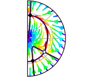
  $n\theta$ of the sphere, as shown in figure 4. Each point in the half-plane represents a unique acoustic mode, and the vector field shows which path the system state will follow as a function of time in the absence of the stochastic contribution of the noise $\sigma$. The solid black lines signify where either of the derivatives are zero, with the zero amplitude derivative $A^{\prime } = 0$ always forming a closed path from $\chi =-{\rm \pi} /4$ to $\chi ={\rm \pi} /4$.
Vector field in the vertical direction ( $n\theta = 0$) for both the conventional FDF ( $R = 1$) and the AFDF ( $R = 1.6$) with ( ${\tilde {\sigma }} = 0.06$) and without ( ${\tilde {\sigma }} = 0$) noise: (a) $R = 1$, ${\tilde {\sigma }} = 0$; (b) $R = 1.6$, ${\tilde {\sigma }} = 0$; (c) $R = 1$, ${\tilde {\sigma }} = 0.06$; (d) $R=1.6$, ${\tilde {\sigma }} = 0.06$. The gain is ${{\tilde {Q}}^{st}} = 0.16 / {\rm \pi}$ and the damping parameter is ${\tilde {\alpha }} = 0.05{{\tilde {Q}}^{st}}$. The solid lines mark $A^{\prime } = 0$ (continuous line from $2\chi =-{\rm \pi} /2$ to $2\chi ={\rm \pi} /2$) and $\chi ^{\prime } = 0$, making the intersections the fixed point locations. Attractors are marked by filled circles and repellors are marked by open circles.

The case in figure 4(a), using the conventional FDF ( $R = 1$) and in the absence of noise ( ${\tilde {\sigma }} = 0$), has three fixed points where both derivatives are zero, one at the standing mode ( $\chi = 0$) and one at each of the spinning modes ( $\chi = \pm {\rm \pi}/4$). The standing solution is an unstable fixed point (open circle marker), while the spinning solutions are stable (filled circle markers), as expected (Schuermans et al. Reference Schuermans, Paschereit and Monkewitz2006; Noiray et al. Reference Noiray, Bothien and Schuermans2011; Ghirardo & Juniper Reference Ghirardo and Juniper2013). In figure 4(b), the same case is shown for $R = 1.6$, which is similar to the value observed in the data in figure 1, illustrating that the change from $R = 1$ to $R = 1.6$ has a distinct effect on the vector field. While the spinning solutions are retained, the unstable fixed point has moved from a purely standing mode to a mixed mode with a CW spinning component ( $\chi < 0$). This increases the basin of attraction of the ACW mode at the expense of the basin of attraction of the CW mode.
Adding noise  ${\tilde {\sigma }} \neq 0$ to the conventional FDF case of $R=1$, the stable spinning solutions $\chi = \pm {\rm \pi}/4$ have been shown to be pushed symmetrically towards standing solutions $\chi ~=~0$ (Ghirardo & Gant Reference Ghirardo and Gant2019; Faure-Beaulieu & Noiray Reference Faure-Beaulieu and Noiray2020; Ghirardo & Gant Reference Ghirardo and Gant2021), as illustrated in figure 4. Figure 4(d) shows that introducing the same noise intensity to the $R=1.6$ case also results in the spinning solutions being pushed away from the vertical axis, but it is not symmetric in this case.
3.1. The effect of damping
The location and number of fixed points are dependent on the parameters of the system, such as the gain  ${{\tilde {Q}}^{st}}$, the damping factor ${\tilde {\alpha }}$ and the noise intensity ${\tilde {\sigma }}$. This is illustrated in figure 5 by varying ${\tilde {\alpha }}$ while keeping ${\tilde {{Q^{st}}}}$ and ${\tilde {\sigma }}$ constant. The size of the loop created by ${\tilde {A}}^{\prime } = 0$ is reduced with an increasing damping factor ${\tilde {\alpha }}$, as the effective gain is reduced. Eventually the curve describing ${\tilde {A}}^{\prime } = 0$ only intersects the $\chi ^{\prime } = 0$ curve once. When this occurs, the initially CW spinning and standing solutions are no longer solutions of the deterministic part of (2.30). This is consistent with the lack of experimental observations of the CW mode at certain operating conditions, including the conditions and set-up where the $R=1.6$ value was obtained (Nygård et al. Reference Nygård, Ghirardo and Worth2021).
Vector field in the vertical direction ( $n\theta = 0$) for an azimuthal flame describing function with $R=1.6$ for different damping values: (a) ${\tilde {\alpha }} = 0.04{{\tilde {Q}}^{st}}$; (b) ${\tilde {\alpha }} = 0.07{{\tilde {Q}}^{st}}$; (c) ${\tilde {\alpha }} = 0.10{{\tilde {Q}}^{st}}$; and (d) ${\tilde {\alpha }} = 0.20{{\tilde {Q}}^{st}}$. The gain and the noise level are ${{\tilde {Q}}^{st}} = 0.16/{\rm \pi}$ and ${\tilde {\sigma }} = 0.06$, respectively. Attractors are marked by filled circles and repellors are marked by open circles. The standing mode and CW spinning solutions are observed to disappear through a saddle node bifurcation as the damping factor ${\tilde {\alpha }}$ is increased.

How the fixed points of the system move, and disappear, as a function of the damping is shown in figure 6 for both  $R=1$ (conventional FDF) and $R=1.6$. Starting with $R=1$ in figure 6(a), the fixed points are observed to move along the lines of $\chi ^{\prime } = 0$ in figure 4. For sufficiently high damping ${\tilde {\alpha }}$, the three fixed points undergo a supercritical pitchfork bifurcation, and a stable standing mode is the only remaining solution. The AFDF with $R = 1.6$ in figure 6(b) has three initial fixed points, a highly spinning stable fixed point for both the ACW and CW direction and an unstable fixed point for mixed modes with a CW component ( $\chi < 0$). As the damping factor ${\tilde {\alpha }}$ is increased, the two fixed points in the southern half-plane meet and annihilate, which is known as a saddle node bifurcation. The initially ACW solution survives, and approaches the standing mode solution for sufficiently high damping ${\tilde {\alpha }}$. In summary, replacing the single-input single-output conventional FDF with the multiple-input single-output AFDF results in different bifurcation behaviour for the system.
Fixed point locations in the vertical plane  $n\theta _{0} = 0$ for a range of different damping values $\alpha$ for (a) the conventional FDF ${\left (R = 1\right )}$ and (b) the AFDF ${\left (R=1.6\right )}$. The gain and noise intensity for both cases are ${{\tilde {Q}}^{st}} = 0.16/{\rm \pi}$ and ${\tilde {\sigma }} = 0.06$, respectively. The conventional FDF results in a supercritical pitchfork bifurcation at sufficiently high damping values ${\tilde {\alpha }}$, while the AFDF case undergoes a saddle node bifurcation for the two fixed points in the southern half.

3.2. Comparison with experiments
A reference case was obtained by operating the atmospheric annular combustor used in Nygård et al. (Reference Nygård, Ghirardo and Worth2021) at an equivalence ratio of  $0.85$ to promote a self-excited thermoacoustic instability. The same 12 injector configuration with swirling flames was used, with the exception of replacing the forcing array with a stainless steel tube to form the outer wall and the new operating condition. Figure 7(a) shows the amplitude $A$ of the acoustic mode for ten repeat cases. Before each run, the combustion chamber is allowed to cool down to approximately 310 K at a reference position on the outer wall, ensuring consistent initial thermal conditions. As the combustion chamber heats up, the mean amplitude is observed to decrease. This coincides with an increasing frequency of the self-excited oscillations, as shown in figure 7(b). The increase in frequency leads to a decrease in the gain ${{\tilde {Q}}^{st}}$, as illustrated for a similar flame in a single injector configuration (Nygård & Worth Reference Nygård and Worth2021), which is consistent with a decrease in amplitude. In combination with the constant fuel and air mixture, the choice is made to simulate the system by decreasing gain values ${{\tilde {Q}}^{st}}$ while keeping the combustion noise ${\tilde {\sigma }}$ and acoustic damping factor ${\tilde {\alpha }}$ constant. In the case where all the flames have the same response, this change of the effective gain ${\left ({{\tilde {Q}}^{st}} - {\tilde {\alpha }}\right )}$ has a similar effect on the amplitude (2.30a) as increasing the damping ${\tilde {\alpha }}$.
Pressure fluctuation amplitude  $A$ (a) and time-dependent frequency spectrum (b) over the whole time series based on the upper measurement location. The instantaneous pressure amplitude is in the background of (a), with the moving mean over ${10}\ {\rm s}$ shown as solid lines. Similarly, the moving mean of the mean frequency is shown as the solid line in (b). The amplitude is observed to steadily decrease in a repeatable manner as the combustor heats up. At the same time, the excitation frequency increases with the increasing temperature.

The time series in figure 7(a) are split into four non-overlapping segments of 10 s each to obtain sections of different mean amplitude. Figure 8(a) shows the joint probability density function of the acoustic amplitude  $A$ and the acoustic nature angle $\chi$ for each segment. Initially, the mode is spinning in the ACW direction and has a relatively large amplitude. Later, as the amplitude decreases, the mode is approximately a standing mode solution. This will be shown to agree with theory for increasing non-dimensional noise in § 3.3, with fixed point paths presented in figure 10. Figure 8(b) shows a simulation using the proposed model with decreasing values of ${{\tilde {Q}}^{st}}$ with the previously used baseline parameter values ${\tilde {\sigma }} = 0.06$, ${\tilde {\alpha }} = 0.032 / {\rm \pi}$ and $R=1.6$. The simulation is run for 170 000 oscillation cycles for each gain value ${Q^{st}}$ to approximately match the number of oscillation cycles observed in the experimental data. All of the simulations are initialised with a standing mode of unit amplitude ${\tilde {A}}$. The simulated mode is observed to be a predominantly ACW mode at relatively high amplitudes for the highest gain value ${Q^{st}} = 5\alpha$, with a similar distribution to the experiment. This can be reproduced by the model in this paper, taking into account the fact that the flames respond more strongly to ACW modes with $R=1.6$. Existing models in the literature ${\left (R=1\right )}$ predict ACW and CW states to be equally dominant, in contrast with the experimental results. This is illustrated in figure 8(c), where all the simulations were started as a standing mode. Likewise, as the gain is reduced, the mode moves closer to the standing mode solution. In both the experiment and the simulation it should be noted that the distribution becomes slightly wider in the angular direction due to the increased non-dimensional noise ${\tilde {\sigma }} / {\tilde {A}}$. This suggests the model is able to capture the general features of the experiment well, even after just manually testing a limited number of parameter combinations.
Joint probability density function for different levels of acoustic perturbations at a fixed operating condition (a) and corresponding simulations using the proposed model (b) and a conventional model (c). The experiment is divided into four non-overlapping time intervals of  ${10}\ {\rm s}$, shown from left to right. The simulations use ${\tilde {\alpha }} = 0.032 / {\rm \pi}$, ${\tilde {\sigma }}=0.06$, ${\tilde {\kappa }} = 6$ and ${{\tilde {Q}}^{st}} = {\left \lbrack 5{\tilde {\alpha }},3.75{\tilde {\alpha }},2.5{\tilde {\alpha }},1.25{\tilde {\alpha }}\right \rbrack }$. Each plot in (b,c) is based on 170 000 oscillation cycles. The proposed model is observed to move towards the standing mode solution ( $\chi = 0$) from the ACW solution, matching the experiments, while both the ACW and CW spinning solutions are observed using a conventional model. There is some slight asymmetry in the results of (c) with respect to the axis at $\chi = 0$ because the underlying distribution is bimodal and the simulation is finite. (a) Experiment, (b) Simulation using the proposed model, $R = 1.6$ and (c) Simulation with conventional models, $R = 1$.

3.3. The effect of noise
When studying the effect of damping or a reduction in gain, in the two previous sections, the non-dimensional noise level  ${\tilde {\sigma }} / {\tilde {A}}$ did increase due to the decrease in the amplitude ${\tilde {A}}$. However, it is also of interest to study the effect of noise for a fixed effective gain, where the noise can grow infinitely large. This effect on the vector field in the vertical direction is shown for a few values of ${\tilde {\sigma }}$ in figure 9. The lowest noise intensity in figure 9(a) yields three solutions, one ACW mode and two closely spaced modes in the southern half-plane. As the noise intensity is increased, the two latter modes are no longer solutions of the system. However, the ACW solution moves to lower nature angles, approaching the standing mode ( $\chi =0$).
Vector field in the vertical direction ( $n\theta = 0$) for an azimuthal flame describing function with $R=1.6$ at different noise levels: (a) ${\tilde {\sigma }}=0.01$; (b) ${\tilde {\sigma }} = 0.06$; (c) ${\tilde {\sigma }} = 0.36$; and (d) ${\tilde {\sigma }}=2.16$. The gain and damping factors are ${{\tilde {Q}}^{st}} = 0.16/{\rm \pi}$ and ${\tilde {\alpha }} = 0.2{{\tilde {Q}}^{st}}$, respectively. Except for the lowest noise level ${\tilde {\sigma }}=0.01$ in (a), the only fixed point is an attractor in the northern half-plane highlighted by the filled circle.

Figure 10(a) shows that the spinning solutions are pushed symmetrically towards the standing solution along the horizontal axis, as expected (Ghirardo & Gant Reference Ghirardo and Gant2019; Faure-Beaulieu & Noiray Reference Faure-Beaulieu and Noiray2020; Ghirardo & Gant Reference Ghirardo and Gant2021). The same illustration is presented for the case of an AFDF with  $R = 1.6$ in figure 10(b). Similarly to the effect in figure 6(b), the two solutions in the southern half meet and annihilate through a saddle node bifurcation, highlighted by the circular marker. The solution starting as a purely ACW spinning mode in the low intensity limit approaches the approximately standing solution, albeit at a much slower rate than in the conventional case due to the $N^{{\left (0\right )}}$ term in (2.30d). For both $R=1$ and for $R=1.6$ in figure 10 the amplitude ${\tilde {A}}$ becomes proportional to the noise intensity ${\tilde {\sigma }}$ at sufficiently high noise intensities. This can also be inferred directly from the equations in (2.30) by letting ${\tilde {\sigma }}$ approach infinity.
Fixed point locations in the vertical plane  $n\theta _{0} = 0$ for a range of different noise intensities ${\tilde {\sigma }}$ for (a) the conventional FDF ${\left (R=1\right )}$ and (b) the AFDF ${\left (R=1.6\right )}$. The gain and damping are ${{\tilde {Q}}^{st}} = 0.16/{\rm \pi}$ and ${\tilde {\alpha }} = 0.2 {{\tilde {Q}}^{st}}$, respectively, for both cases. At sufficiently high noise intensities, the solution approaches the standing mode for both cases, albeit at a slower rate for the $R=1.6$ case in (b). In both cases the fixed points initially closest to the spinning solutions are attractors (solid line) while the third fixed point is a repellor (dashed line).

4. Conclusion
The current study successfully implemented the multiple-input single-output AFDF in a quaternion valued low-order model of an annular combustion chamber. To achieve this, the AFDF was reformulated from the orthogonal spinning mode decomposition to a quaternion-based expression with amplitude, orientation angle, nature angle and temporal phase as state space parameters. The heat release rate mode and of the acoustic mode parameters are linked through explicit expressions, meaning only one set of parameters needs to be solved for. The different response of the flames to acoustic waves of opposite spinning directions is described by the gain ratio  $R$ between the two components of the AFDF. The conventional model using the single-input single-output FDF is recovered in the special case $R=1$.
Conventional FDF models often saturate the response as a function of the local acoustic field amplitude. Since the AFDF does not assume the heat release rate and acoustic modes have the same nature angle, a new amplitude reference for saturation was required to avoid unconstrained growth of the heat release rate at pressure node locations at large acoustic amplitudes. The new amplitude reference was proposed to be the linear heat release rate amplitude  $A_{q}$. One specific nonlinear saturation function is applied to it, without full experimental validation because of the absence of experimental data at sufficiently high amplitudes to evaluate this. However, a sensitivity analysis demonstrated that the results are qualitatively transferable to other choices of the saturation functions, especially if they are monotonic.
One of the main features of the AFDF is the difference in nature angle  $\Delta \chi$ between the heat release rate mode and the acoustic mode. For the conventional FDF case, the mean heat release rate term only affects the equation for the amplitude $A$, but $\Delta \chi \neq 0$ for the AFDF case results in a contribution from the mean heat release rate to the equation for the nature angle $\chi$ as well. This redistribution has a significant effect on the vector fields in the $A$–
$A$– $2\chi$-plane. For certain parameter combinations there are three solutions, two strongly spinning stable solutions in opposite directions and a third unstable solution in between, similar to the case for the conventional FDF. However, the initially CW spinning (for $R > 1$) solution and the unstable solution can meet and disappear through a saddle node bifurcation. This can for example happen when the acoustic damping of the system is increased, or when the noise level is increased, matching experimental evidence that a CW mode is never observed at certain operating conditions. The standing mode is retained as the only solution in the infinite noise limit for both the FDF and the AFDF case.
Experiments at a fixed fuel and air flow showed that, as the linear gain decreases as a function of increasing frequency, the mode is pushed away from the purely spinning state and the amplitude decreases, as expected from the model. It is shown to qualitatively model the experimental results well, showing the same main features.
Supplementary material
Supplementary material is available at https://doi.org/10.1017/jfm.2023.921. The numerical implementation of the model is available under MIT license at https://doi.org/10.5281/zenodo.10071467 (Nygård Reference Nygård2023).
Funding
The authors would like to acknowledge financial support from the Norwegian Research Council, project no. 299946.
Declaration of interests
The authors report no conflict of interest.
Appendix A. Heat release rate integral
The model presented in Ghirardo & Gant (Reference Ghirardo and Gant2021) without the effect of the stochastic noise can be expressed as
 \begin{equation} r^{\prime} + r{\mathrm{j}}\varphi^{\prime} = {\left(-\frac{\omega}{2} + \frac{\omega_{0}^{2}}{2\omega}\right)}r{\mathrm{j}} + \frac{1}{2}\frac{1}{2{\rm \pi}/\omega}\int_{0}^{2{\rm \pi}/\omega} \mathcal{F} \exp({-{\mathrm{j}}{\left({\omega t + \varphi}\right)}})\,\mathrm{d}t, \end{equation}
where the following notational shorthands have been introduced:
 \begin{gather} r = A\exp({{\mathrm{i}} n\theta_{0}})\exp({-{\mathrm{k}} \chi}), \end{gather}
 \begin{gather}r^{\prime} = A^{\prime}\exp({{\mathrm{i}} n\theta_{0}})\exp({{\mathrm{k}} \chi}) + A{\mathrm{i}} n\theta_{0}^{\prime} \exp({{\mathrm{i}} n\theta_{0}})\exp({{\mathrm{k}} \chi}) - A\exp({{\mathrm{i}} n\theta_{0}}) \exp({{\mathrm{k}} \chi}){\mathrm{k}}\chi^{\prime}, \end{gather}
 \begin{gather}\mathcal{F} = \frac{2}{\rm \pi}\int_{0}^{2{\rm \pi}}\exp({{\mathrm{i}} n\theta})q\,\mathrm{d}\theta. \end{gather}
Since the equation is quaternion valued, the terms do not commute in general, and care has to be taken when rearranging terms. Following the derivation of Ghirardo & Gant (Reference Ghirardo and Gant2021), (A1) is multiplied by  $\exp ({-{\mathrm {i}} n\theta _{0}})$ on the left and by $\exp ({{\mathrm {k}}\chi })$ on the right to obtain
 \begin{align} \exp({-{\mathrm{i}}
n\theta_{0}})&{(r^{\prime} + \exp({-{\mathrm{i}} n\theta_{0}})
r{\mathrm{j}}\varphi^{\prime})}\exp({{\mathrm{k}}\chi})
\nonumber\\ &= \exp({-{\mathrm{i}}
n\theta_{0}}){\left(-\frac{\omega}{2} +
\frac{\omega_{0}^{2}}{2\omega}\right)}r{\mathrm{j}}
\exp({{\mathrm{k}}\chi}) \nonumber\\ &\quad+
\exp({-{\mathrm{i}} n\theta_{0}})
\frac{1}{2}\frac{1}{2{\rm \pi}/\omega}\int_{0}^{2{\rm \pi}/\omega}
\mathcal{F} \exp({-{\mathrm{j}}{\left({\omega t +
\varphi}\right)}})\,\mathrm{d}t\exp({{\mathrm{k}}\chi}).
\end{align}
\begin{align} \exp({-{\mathrm{i}}
n\theta_{0}})&{(r^{\prime} + \exp({-{\mathrm{i}} n\theta_{0}})
r{\mathrm{j}}\varphi^{\prime})}\exp({{\mathrm{k}}\chi})
\nonumber\\ &= \exp({-{\mathrm{i}}
n\theta_{0}}){\left(-\frac{\omega}{2} +
\frac{\omega_{0}^{2}}{2\omega}\right)}r{\mathrm{j}}
\exp({{\mathrm{k}}\chi}) \nonumber\\ &\quad+
\exp({-{\mathrm{i}} n\theta_{0}})
\frac{1}{2}\frac{1}{2{\rm \pi}/\omega}\int_{0}^{2{\rm \pi}/\omega}
\mathcal{F} \exp({-{\mathrm{j}}{\left({\omega t +
\varphi}\right)}})\,\mathrm{d}t\exp({{\mathrm{k}}\chi}).
\end{align}
The only term of interest for the implementation of the AFDF into the model is the last term on the right-hand side:
 \begin{equation} \mathscr{I} = \exp({-{\mathrm{i}} n\theta_{0}})\frac{1}{2}\frac{1}{2{\rm \pi}/\omega}\int_{0}^{2{\rm \pi}/\omega} \frac{1}{\rm \pi}\int_{0}^{2{\rm \pi}}\exp({{\mathrm{i}} n\theta})2q\,\mathrm{d}\theta\exp({-{\mathrm{j}}{\left({\omega t + \varphi}\right)}})\,\mathrm{d}t\exp({{\mathrm{k}}\chi}). \end{equation}
The order of integration can be switched for this expression, yielding
 \begin{equation} \mathscr{I} = \frac{1}{2{\rm \pi}}\int_{0}^{2{\rm \pi}}\exp({{\mathrm{i}} {n{\left(\theta - \theta_{0}\right)}}})\frac{1}{2{\rm \pi}/\omega}\int_{0}^{2{\rm \pi}/\omega}2q\exp({-{\mathrm{j}}{\left({\omega t + \varphi}\right)}})\, \mathrm{d}t\,\mathrm{d}\theta\exp({{\mathrm{k}}\chi}). \end{equation}
The inner integral
 \begin{equation} \mathcal{I} = \frac{1}{2{\rm \pi}/\omega}\int_{0}^{2{\rm \pi}/\omega}2q\exp({-{\mathrm{j}}{\left({\omega t + \varphi}\right)}})\,\mathrm{d}t, \end{equation}
can be computed analytically, as the slowly varying state space variables are assumed to be constant in time over the acoustic period  $2{\rm \pi} / \omega$. The real valued heat release rate $q$ is given by (2.24), which can be written as
 \begin{equation} 2q = \hat{Q}{{\rm e}^{{\mathrm{j}}\omega t}} + \text{q.c.} = \hat{Q}{{\rm e}^{{\mathrm{j}}\omega t}} + {{\rm e}^{-{\mathrm{j}}\omega t}}\hat{Q}^{{\ast}}, \end{equation}
where  $\hat {Q}$ is a shorthand for the slowly varying terms in the original expression. Inserting into the inner integral yields
 \begin{align}
\mathcal{I} & = \frac{1}{2{\rm \pi}/\omega}\int_{0}^{2{\rm \pi}/\omega}{\lbrack
\hat{Q}\exp(\kern0.7pt {{\mathrm{j}}\omega t}) +
\exp({-{\mathrm{j}}\omega
t})\hat{Q}^{{\ast}}\rbrack}\exp({-{\mathrm{j}}{({\omega
t + \varphi})}})\,\mathrm{d}t, \nonumber\\
& = \frac{1}{2{\rm \pi}/\omega}\int_{0}^{2{\rm \pi}/\omega}{\lbrack
\hat{Q}\exp({-{\mathrm{j}}\varphi}) +
\exp({-{\mathrm{j}}{({\omega t +
\varphi})}})\exp(\kern0.7pt
{{\mathrm{j}}\varphi})\hat{Q}^{{\ast}}
\exp({-{\mathrm{j}}{({\omega t +
\varphi})}})\rbrack}\mathrm{d}t, \nonumber\\ &
=
\frac{1}{2{\rm \pi}/\omega}\int_{0}^{2{\rm \pi}/\omega}{\lbrack
\hat{Q}\exp({-{\mathrm{j}}\varphi}) +
\exp({-{\mathrm{j}}{\left({\omega t +
\varphi}\right)}}){(\hat{Q}\exp({-{\mathrm{j}}\varphi}))}^{{\ast}}
\exp({-{\mathrm{j}}{({\omega t +
\varphi})}})\rbrack}\mathrm{d}t, \nonumber\\ &
= \frac{{(\hat{Q}\exp({-{\mathrm{j}}\varphi}))}
-
{\mathrm{j}}{(\hat{Q}\exp({-{\mathrm{j}}\varphi}))}{\mathrm{j}}}{2},
\end{align}
\begin{align}
\mathcal{I} & = \frac{1}{2{\rm \pi}/\omega}\int_{0}^{2{\rm \pi}/\omega}{\lbrack
\hat{Q}\exp(\kern0.7pt {{\mathrm{j}}\omega t}) +
\exp({-{\mathrm{j}}\omega
t})\hat{Q}^{{\ast}}\rbrack}\exp({-{\mathrm{j}}{({\omega
t + \varphi})}})\,\mathrm{d}t, \nonumber\\
& = \frac{1}{2{\rm \pi}/\omega}\int_{0}^{2{\rm \pi}/\omega}{\lbrack
\hat{Q}\exp({-{\mathrm{j}}\varphi}) +
\exp({-{\mathrm{j}}{({\omega t +
\varphi})}})\exp(\kern0.7pt
{{\mathrm{j}}\varphi})\hat{Q}^{{\ast}}
\exp({-{\mathrm{j}}{({\omega t +
\varphi})}})\rbrack}\mathrm{d}t, \nonumber\\ &
=
\frac{1}{2{\rm \pi}/\omega}\int_{0}^{2{\rm \pi}/\omega}{\lbrack
\hat{Q}\exp({-{\mathrm{j}}\varphi}) +
\exp({-{\mathrm{j}}{\left({\omega t +
\varphi}\right)}}){(\hat{Q}\exp({-{\mathrm{j}}\varphi}))}^{{\ast}}
\exp({-{\mathrm{j}}{({\omega t +
\varphi})}})\rbrack}\mathrm{d}t, \nonumber\\ &
= \frac{{(\hat{Q}\exp({-{\mathrm{j}}\varphi}))}
-
{\mathrm{j}}{(\hat{Q}\exp({-{\mathrm{j}}\varphi}))}{\mathrm{j}}}{2},
\end{align}
where the last step used an integral relation shown by Ghirardo & Gant (Reference Ghirardo and Gant2021) to hold for any function, such as  $\hat {Q}{{\rm e}^{-{\mathrm {j}}\varphi }}$, which is independent of the integration variable.
Finally, inserting for  $\widehat {{Q_{\theta }}}$ into the expression for $\mathcal {I}$ yields
 \begin{align} \mathcal{I} &=
\frac{A}{2}{\lbrack
\exp({{\mathrm{i}}{n{(\theta - \theta_{0,
q})}}})\exp({{\mathrm{k}}\chi_{q}{(A,
\chi)}}) + \exp({-{\mathrm{i}}{n{(\theta - \theta_{0, q})}}})\exp({-{\mathrm{k}}\chi_{q}{(A,
\chi)}})\rbrack}\nonumber\\ &\quad
\times{Q_{\theta}}{(A, \chi, \theta,
\theta_{0})}\exp(\kern0.7pt
{{\mathrm{j}}\bar{\phi}_{q}{(A,\chi)}}),
\end{align}
\begin{align} \mathcal{I} &=
\frac{A}{2}{\lbrack
\exp({{\mathrm{i}}{n{(\theta - \theta_{0,
q})}}})\exp({{\mathrm{k}}\chi_{q}{(A,
\chi)}}) + \exp({-{\mathrm{i}}{n{(\theta - \theta_{0, q})}}})\exp({-{\mathrm{k}}\chi_{q}{(A,
\chi)}})\rbrack}\nonumber\\ &\quad
\times{Q_{\theta}}{(A, \chi, \theta,
\theta_{0})}\exp(\kern0.7pt
{{\mathrm{j}}\bar{\phi}_{q}{(A,\chi)}}),
\end{align}
where the explicit mode dependence of  $\theta _{0, q}$ has been temporarily dropped for notational convenience. This expression can then be used to obtain the source term $\mathscr {I}$ from the heat release rate fluctuations
 \begin{align} \mathscr{I} &=
\frac{A}{2}\frac{1}{2{\rm \pi}}\int_{0}^{2{\rm \pi}}
(\exp({2{\mathrm{i}}{n{(\theta -
\theta_{0})}}})
\exp({-{\mathrm{i}}{\Delta\phi_{q}}{(A,
\chi)}})\exp({{\mathrm{k}}\chi_{q}{(A,
\chi)}}) \nonumber\\ &\quad
+\exp({{\mathrm{i}}{\Delta\phi_{q}}{(A,
\chi)}})\exp({-{\mathrm{k}}\chi_{q}{(A,
\chi)}})) {Q_{\theta}}{(A, \chi, \theta, \theta_{0})} \exp(\kern0.7pt
{{\mathrm{j}}\bar{\phi}_{q}{(A,\chi)}})
\,\mathrm{d}\theta\exp({{\mathrm{k}}\chi}).
\end{align}
\begin{align} \mathscr{I} &=
\frac{A}{2}\frac{1}{2{\rm \pi}}\int_{0}^{2{\rm \pi}}
(\exp({2{\mathrm{i}}{n{(\theta -
\theta_{0})}}})
\exp({-{\mathrm{i}}{\Delta\phi_{q}}{(A,
\chi)}})\exp({{\mathrm{k}}\chi_{q}{(A,
\chi)}}) \nonumber\\ &\quad
+\exp({{\mathrm{i}}{\Delta\phi_{q}}{(A,
\chi)}})\exp({-{\mathrm{k}}\chi_{q}{(A,
\chi)}})) {Q_{\theta}}{(A, \chi, \theta, \theta_{0})} \exp(\kern0.7pt
{{\mathrm{j}}\bar{\phi}_{q}{(A,\chi)}})
\,\mathrm{d}\theta\exp({{\mathrm{k}}\chi}).
\end{align}
The above expression is the same as the one obtained by Ghirardo & Gant (Reference Ghirardo and Gant2021) for the conventional FDF except for the introduction of the heat release rate mode nature angle  $\chi _{q}$ instead of the nature angle $\chi$ of the acoustic pressure mode and the introduction of the phase difference $\Delta \phi _{q}$. Additionally, the functional form of the describing function ${Q_{\theta }}$ has an explicit nature angle dependence (which was also possible to account for in the original derivation Ghirardo & Gant Reference Ghirardo and Gant2021).
Appendix B. Full governing equation
The main governing equation in (2.30) without the simplifying assumption  $\bar {\phi }_{q} = {\Delta \phi _{q}} = 0$ can be obtained from (2.26) and (2.29)
 \begin{align}
\frac{A^{\prime}}{A} &=
\frac{M}{2}N^{{(0)}}{\lbrack
{\cos{({\Delta\phi_{q}})}}{\cos{(\chi_{q})}}{\cos{(\bar{\phi}_{q})}}
- {\sin{({\Delta\phi_{q}})}}{\sin{(\chi_{q})}}{\sin{(\bar{\phi}_{q})}}\rbrack}{\cos{(\chi)}}\nonumber\\
&\quad +\frac{M}{2}N^{{(0)}}{\lbrack
{\cos{({\Delta\phi_{q}})}}{\sin{(\chi_{q})}}{\cos{(\bar{\phi}_{q})}}
- {\sin{({\Delta\phi_{q}})}}{\cos{(\chi_{q})}}{\sin{(\bar{\phi}_{q})}}\rbrack}{\sin{\left(\chi\right)}}\nonumber\\
&\quad +\frac{M}{4}N^{{(2n)}}[{\cos{(2n\theta^{{(2n)}} + {\Delta\phi_{q}})}}
{\cos{(\chi_{q})}}{\cos{(\bar{\phi}_{q})}} \nonumber\\ &\quad + {\sin{(2n\theta^{{(2n)}} +
{\Delta\phi_{q}})}}{\sin{(\chi_{q})}}{\sin{(\bar{\phi}_{q})}}]{\cos{\left(\chi\right)}}\nonumber\\
&\quad -\frac{M}{4}N^{{(2n)}}[{\cos{(2n\theta^{{(2n)}} + {\Delta\phi_{q}})}}{\sin{(\chi_{q})}}{\cos{(\bar{\phi}_{q})}}\nonumber\\
&\quad + \,{\sin{(2n\theta^{{(2n)}} + {\Delta\phi_{q}})}}{\cos{(\chi_{q})}}{\sin{(\bar{\phi}_{q})}}]{\sin{(\chi)}}\nonumber\\
&\quad -\frac{M}{2}\alpha + \frac{\sigma^{2}}{4A^{2}} + \frac{\sigma}{\sqrt{2}A}\mu_{0}\end{align}
\begin{align}
\frac{A^{\prime}}{A} &=
\frac{M}{2}N^{{(0)}}{\lbrack
{\cos{({\Delta\phi_{q}})}}{\cos{(\chi_{q})}}{\cos{(\bar{\phi}_{q})}}
- {\sin{({\Delta\phi_{q}})}}{\sin{(\chi_{q})}}{\sin{(\bar{\phi}_{q})}}\rbrack}{\cos{(\chi)}}\nonumber\\
&\quad +\frac{M}{2}N^{{(0)}}{\lbrack
{\cos{({\Delta\phi_{q}})}}{\sin{(\chi_{q})}}{\cos{(\bar{\phi}_{q})}}
- {\sin{({\Delta\phi_{q}})}}{\cos{(\chi_{q})}}{\sin{(\bar{\phi}_{q})}}\rbrack}{\sin{\left(\chi\right)}}\nonumber\\
&\quad +\frac{M}{4}N^{{(2n)}}[{\cos{(2n\theta^{{(2n)}} + {\Delta\phi_{q}})}}
{\cos{(\chi_{q})}}{\cos{(\bar{\phi}_{q})}} \nonumber\\ &\quad + {\sin{(2n\theta^{{(2n)}} +
{\Delta\phi_{q}})}}{\sin{(\chi_{q})}}{\sin{(\bar{\phi}_{q})}}]{\cos{\left(\chi\right)}}\nonumber\\
&\quad -\frac{M}{4}N^{{(2n)}}[{\cos{(2n\theta^{{(2n)}} + {\Delta\phi_{q}})}}{\sin{(\chi_{q})}}{\cos{(\bar{\phi}_{q})}}\nonumber\\
&\quad + \,{\sin{(2n\theta^{{(2n)}} + {\Delta\phi_{q}})}}{\cos{(\chi_{q})}}{\sin{(\bar{\phi}_{q})}}]{\sin{(\chi)}}\nonumber\\
&\quad -\frac{M}{2}\alpha + \frac{\sigma^{2}}{4A^{2}} + \frac{\sigma}{\sqrt{2}A}\mu_{0}\end{align}
 \begin{align} & n\theta^{\prime} +
\varphi^{\prime}\sin{(2\chi)} \nonumber\\
&\quad = \frac{\sigma}{\sqrt{2}A}\mu_{1}+ \frac{M}{2}N^{{(0)}}
{\lbrack{\sin{({\Delta\phi_{q}})}}{\sin{(\chi_{q})}}{\cos{(\bar{\phi}_{q})}}
+ {\cos{({\Delta\phi_{q}})}}{\cos{(\chi_{q})}}{\sin{(\bar{\phi}_{q})}}\rbrack}{\sin{(\chi)}}\nonumber\\
&\qquad + \frac{M}{2}N^{{(0)}}{\lbrack {\sin{({\Delta\phi_{q}})}}{\cos{(\chi_{q})}}{\cos{(\bar{\phi}_{q})}}
+ {\sin{({\Delta\phi_{q}})}}{\cos{(\chi_{q})}}{\sin{(\bar{\phi}_{q})}}\rbrack}{\cos{(\chi)}}\nonumber\\
&\qquad - \frac{M}{4}N^{{(2n)}}[{\sin{(2n\theta^{{(2n)}}
+ {\Delta\phi_{q}})}}{\sin{(\chi_{q})}}{\cos{(\bar{\phi}_{q})}} \nonumber\\ &\qquad -{\cos{(2n\theta^{{(2n)}} +
{\Delta\phi_{q}})}}{\cos{(\chi_{q})}}{\sin{(\bar{\phi}_{q})}}]{\sin{(\chi)}}\nonumber\\
&\qquad + \frac{M}{4}N^{{(2n)}}[{\sin{(2n\theta^{{(2n)}} +
{\Delta\phi_{q}})}}{\cos{(\chi_{q})}}{\cos{(\bar{\phi}_{q})}} \nonumber\\ &\qquad -\,
{\sin{(2n\theta^{{(2n)}} + {\Delta\phi_{q}})}}{\cos{(\chi_{q})}}{\sin{(\bar{\phi}_{q})}}]{\cos{(\chi)}}
\end{align}
\begin{align} & n\theta^{\prime} +
\varphi^{\prime}\sin{(2\chi)} \nonumber\\
&\quad = \frac{\sigma}{\sqrt{2}A}\mu_{1}+ \frac{M}{2}N^{{(0)}}
{\lbrack{\sin{({\Delta\phi_{q}})}}{\sin{(\chi_{q})}}{\cos{(\bar{\phi}_{q})}}
+ {\cos{({\Delta\phi_{q}})}}{\cos{(\chi_{q})}}{\sin{(\bar{\phi}_{q})}}\rbrack}{\sin{(\chi)}}\nonumber\\
&\qquad + \frac{M}{2}N^{{(0)}}{\lbrack {\sin{({\Delta\phi_{q}})}}{\cos{(\chi_{q})}}{\cos{(\bar{\phi}_{q})}}
+ {\sin{({\Delta\phi_{q}})}}{\cos{(\chi_{q})}}{\sin{(\bar{\phi}_{q})}}\rbrack}{\cos{(\chi)}}\nonumber\\
&\qquad - \frac{M}{4}N^{{(2n)}}[{\sin{(2n\theta^{{(2n)}}
+ {\Delta\phi_{q}})}}{\sin{(\chi_{q})}}{\cos{(\bar{\phi}_{q})}} \nonumber\\ &\qquad -{\cos{(2n\theta^{{(2n)}} +
{\Delta\phi_{q}})}}{\cos{(\chi_{q})}}{\sin{(\bar{\phi}_{q})}}]{\sin{(\chi)}}\nonumber\\
&\qquad + \frac{M}{4}N^{{(2n)}}[{\sin{(2n\theta^{{(2n)}} +
{\Delta\phi_{q}})}}{\cos{(\chi_{q})}}{\cos{(\bar{\phi}_{q})}} \nonumber\\ &\qquad -\,
{\sin{(2n\theta^{{(2n)}} + {\Delta\phi_{q}})}}{\cos{(\chi_{q})}}{\sin{(\bar{\phi}_{q})}}]{\cos{(\chi)}}
\end{align}
 \begin{align} &
\varphi^{\prime}\cos{(2\chi)}\nonumber\\ &\quad =
\frac{\sigma}{\sqrt{2}A}\mu_{2} +
\frac{M}{2}N^{{(0)}}{\lbrack
{\sin{({\Delta\phi_{q}})}}{\sin{(\chi_{q})}}{\cos{(\bar{\phi}_{q})}}
+
{\cos{({\Delta\phi_{q}})}}{\cos{(\chi_{q})}}{\sin{(\bar{\phi}_{q})}}\rbrack}{\cos{(\chi)}}\nonumber\\
&\qquad - \frac{M}{2}N^{{(0)}}{\lbrack
{\sin{({\Delta\phi_{q}})}}{\cos{(\chi_{q})}}{\cos{(\bar{\phi}_{q})}}
+
{\sin{({\Delta\phi_{q}})}}{\cos{(\chi_{q})}}{\sin{(\bar{\phi}_{q})}}\rbrack}{\sin{(\chi)}}\nonumber\\
&\qquad - \frac{M}{4}N^{{(2n)}}[{\sin{(2n\theta^{{(2n)}} +
{\Delta\phi_{q}})}}{\sin{(\chi_{q})}}{\cos{(\bar{\phi}_{q})}} \nonumber\\ &\qquad -\, {\cos{(2n\theta^{{(2n)}} +
{\Delta\phi_{q}})}}{\cos{(\chi_{q})}}{\sin{(\bar{\phi}_{q})}}]{\cos{(\chi)}}\nonumber\\
&\qquad - \frac{M}{4}N^{{(2n)}}[{\sin{(2n\theta^{{(2n)}} +
{\Delta\phi_{q}})}}{\cos{(\chi_{q})}}{\cos{(\bar{\phi}_{q})}} \nonumber\\ &\qquad -\, {\sin{(2n\theta^{{(2n)}} +
{\Delta\phi_{q}})}}{\cos{(\chi_{q})}}{\sin{(\bar{\phi}_{q})}}]{\sin{(\chi)}}
\end{align}
\begin{align} &
\varphi^{\prime}\cos{(2\chi)}\nonumber\\ &\quad =
\frac{\sigma}{\sqrt{2}A}\mu_{2} +
\frac{M}{2}N^{{(0)}}{\lbrack
{\sin{({\Delta\phi_{q}})}}{\sin{(\chi_{q})}}{\cos{(\bar{\phi}_{q})}}
+
{\cos{({\Delta\phi_{q}})}}{\cos{(\chi_{q})}}{\sin{(\bar{\phi}_{q})}}\rbrack}{\cos{(\chi)}}\nonumber\\
&\qquad - \frac{M}{2}N^{{(0)}}{\lbrack
{\sin{({\Delta\phi_{q}})}}{\cos{(\chi_{q})}}{\cos{(\bar{\phi}_{q})}}
+
{\sin{({\Delta\phi_{q}})}}{\cos{(\chi_{q})}}{\sin{(\bar{\phi}_{q})}}\rbrack}{\sin{(\chi)}}\nonumber\\
&\qquad - \frac{M}{4}N^{{(2n)}}[{\sin{(2n\theta^{{(2n)}} +
{\Delta\phi_{q}})}}{\sin{(\chi_{q})}}{\cos{(\bar{\phi}_{q})}} \nonumber\\ &\qquad -\, {\cos{(2n\theta^{{(2n)}} +
{\Delta\phi_{q}})}}{\cos{(\chi_{q})}}{\sin{(\bar{\phi}_{q})}}]{\cos{(\chi)}}\nonumber\\
&\qquad - \frac{M}{4}N^{{(2n)}}[{\sin{(2n\theta^{{(2n)}} +
{\Delta\phi_{q}})}}{\cos{(\chi_{q})}}{\cos{(\bar{\phi}_{q})}} \nonumber\\ &\qquad -\, {\sin{(2n\theta^{{(2n)}} +
{\Delta\phi_{q}})}}{\cos{(\chi_{q})}}{\sin{(\bar{\phi}_{q})}}]{\sin{(\chi)}}
\end{align}
 \begin{align} - \chi^{\prime} &=
\frac{\sigma^{2}}{4A^{2}}\tan{(2\chi)} +
\frac{\sigma}{\sqrt{2}A}\mu_{3}\nonumber\\ &\quad +
\frac{M}{2}N^{{(0)}}{\lbrack
{\cos{({\Delta\phi_{q}})}}{\cos{(\chi_{q})}}{\cos{(\bar{\phi}_{q})}}
-
{\sin{({\Delta\phi_{q}})}}{\sin{(\chi_{q})}}{\sin{(\bar{\phi}_{q})}}\rbrack}{\sin{(\chi)}}\nonumber\\
&\quad + \frac{M}{2}N^{{(0)}}{\lbrack
{\sin{({\Delta\phi_{q}})}}{\cos{(\chi_{q})}}{\sin{(\bar{\phi}_{q})}}
-
{\sin{({\Delta\phi_{q}})}}{\cos{(\chi_{q})}}{\cos{(\bar{\phi}_{q})}}\rbrack}{\cos{(\chi)}}\nonumber\\
&\quad + \frac{M}{4}N^{{(2n)}}[{\cos{(2n\theta^{{(2n)}} +
{\Delta\phi_{q}})}}{\cos{(\chi_{q})}}{\cos{(\bar{\phi}_{q})}}
\nonumber\\ &\quad +\, {\sin{(2n\theta^{{(2n)}} +
{\Delta\phi_{q}})}}{\sin{(\chi_{q})}}{\sin{(\bar{\phi}_{q})}}]{\sin{(\chi)}}\nonumber\\
&\quad + \frac{M}{4}N^{{(2n)}}[{\sin{(2n\theta^{{(2n)}} +
{\Delta\phi_{q}})}}{\cos{(\chi_{q})}}{\sin{(\bar{\phi}_{q})}}
\nonumber\\ &\quad + \,{\sin{(2n\theta^{{(2n)}} +
{\Delta\phi_{q}})}}{\cos{(\chi_{q})}}{\cos{(\bar{\phi}_{q})}}]{\cos{(\chi)}}.
\end{align}
\begin{align} - \chi^{\prime} &=
\frac{\sigma^{2}}{4A^{2}}\tan{(2\chi)} +
\frac{\sigma}{\sqrt{2}A}\mu_{3}\nonumber\\ &\quad +
\frac{M}{2}N^{{(0)}}{\lbrack
{\cos{({\Delta\phi_{q}})}}{\cos{(\chi_{q})}}{\cos{(\bar{\phi}_{q})}}
-
{\sin{({\Delta\phi_{q}})}}{\sin{(\chi_{q})}}{\sin{(\bar{\phi}_{q})}}\rbrack}{\sin{(\chi)}}\nonumber\\
&\quad + \frac{M}{2}N^{{(0)}}{\lbrack
{\sin{({\Delta\phi_{q}})}}{\cos{(\chi_{q})}}{\sin{(\bar{\phi}_{q})}}
-
{\sin{({\Delta\phi_{q}})}}{\cos{(\chi_{q})}}{\cos{(\bar{\phi}_{q})}}\rbrack}{\cos{(\chi)}}\nonumber\\
&\quad + \frac{M}{4}N^{{(2n)}}[{\cos{(2n\theta^{{(2n)}} +
{\Delta\phi_{q}})}}{\cos{(\chi_{q})}}{\cos{(\bar{\phi}_{q})}}
\nonumber\\ &\quad +\, {\sin{(2n\theta^{{(2n)}} +
{\Delta\phi_{q}})}}{\sin{(\chi_{q})}}{\sin{(\bar{\phi}_{q})}}]{\sin{(\chi)}}\nonumber\\
&\quad + \frac{M}{4}N^{{(2n)}}[{\sin{(2n\theta^{{(2n)}} +
{\Delta\phi_{q}})}}{\cos{(\chi_{q})}}{\sin{(\bar{\phi}_{q})}}
\nonumber\\ &\quad + \,{\sin{(2n\theta^{{(2n)}} +
{\Delta\phi_{q}})}}{\cos{(\chi_{q})}}{\cos{(\bar{\phi}_{q})}}]{\cos{(\chi)}}.
\end{align}


 Open access