2.1. Governing equations

We used the inclined layer convection (ILC) extension module of the MPI-parallel pseudo-spectral code Channelflow 2.0 (Reetz Reference Reetz2019; Gibson et al. Reference Gibson, Reetz, Azimi, Ferraro, Kreilos, Schrobsdorff, Farano, Yesil, Schütz and Culpo2021) to carry out DNS of the non-dimensionalized Oberbeck–Boussinesq equations

(2.1a)$$\begin{gather} \dfrac{\partial \boldsymbol{u}}{\partial t} + (\boldsymbol{u} \boldsymbol{\cdot}\boldsymbol{\nabla}) \boldsymbol{u} ={-}\boldsymbol{\nabla} p + \sqrt{\frac{Pr}{Ra}}\,\nabla^2 \boldsymbol{u} + \mathcal{T}\boldsymbol{e}_z, \end{gather}$$

(2.1b)$$\begin{gather}\dfrac{\partial \mathcal{T}}{\partial t} + (\boldsymbol{u}\boldsymbol{\cdot}\boldsymbol{\nabla}) \mathcal{T} = \frac{1}{\sqrt{Pr\,Ra}}\,\nabla^2 \mathcal{T}, \end{gather}$$

(2.1c)$$\begin{gather}\boldsymbol{\nabla}\boldsymbol{\cdot}\boldsymbol{u}= 0, \end{gather}$$

in a vertical channel as depicted in figure 1. In (2.1), $\boldsymbol {u} = [u, v, w](x,y,z,t)$ and $\mathcal {T}=\mathcal {T}(x,y,z,t)$ stand for total velocity and temperature, respectively. The constant buoyancy term has been omitted from (2.1a); correspondingly, the pressure $p=p(x,y,z,t)$ is relative to the hydrostatic pressure. Bold symbols denote vector quantities, and $\boldsymbol {e}_z$ is the vertical unit vector. The equations have been non-dimensionalized with respect to the temperature difference $\Delta \vartheta$ and the distance $W$ between the walls, and the free-fall time unit $(W/g\alpha \,\Delta \vartheta )^{1/2}$, where $\alpha$ is the thermal expansion coefficient, and $g$ is the gravitational acceleration. Two independent dimensionless parameters appear: Rayleigh number $Ra = g \alpha \,\Delta \vartheta \, W^3/(\nu \kappa )$ and Prandtl number $Pr = \nu /\kappa$, where $\nu$ is the kinematic viscosity, and $\kappa$ is the thermal diffusivity.

Periodic boundary conditions are imposed in the $y$ and $z$ directions with spatial periods $L_y$ and $L_z$, respectively. The walls are no-slip and have prescribed temperatures

(2.2a,b)\begin{equation} \boldsymbol{u}(x={\pm} 0.5) = 0,\quad \mathcal{T}(x=\pm0.5)=\pm0.5. \end{equation}

A supplementary integral constraint on either the pressure gradient or the mean flux must be set in the periodic directions. In order to match the simulations of Gao et al. (Reference Gao, Sergent, Podvin, Xin, Le Quéré and Tuckerman2013, Reference Gao, Podvin, Sergent and Xin2015, Reference Gao, Podvin, Sergent, Xin and Chergui2018), we impose a mean pressure gradient of zero in $y$ and in $z$. Equations (2.1) together with the boundary conditions admit the conductive solution sketched in figure 1(a):

(2.3a)$$\begin{gather} \boldsymbol{u}_0(x) = \frac{1}{6}\,\sqrt{\frac{Ra}{Pr}} \left(\frac{1}{4}\,x - x^3 \right) \boldsymbol{e}_z, \end{gather}$$

(2.3b)$$\begin{gather}\mathcal{T}_0(x) = x, \end{gather}$$

(2.3c)$$\begin{gather}p_0(x) = \varPi, \end{gather}$$

with arbitrary pressure constant $\varPi$.

2.2. Numerical methods

Channelflow-ILC adopts Chebychev–Fourier–Fourier (in $x$, $y$ and $z$) expansions for representing flow fields in space, and a finite differencing method for time integration (see detailed description in Appendix A of Reetz & Schneider Reference Reetz and Schneider2020). We have simulated the three-dimensional computational domain studied in Gao et al. (Reference Gao, Sergent, Podvin, Xin, Le Quéré and Tuckerman2013). This narrow domain $[L_x, L_y, L_z] = [1, 1, 10]$ is discretized by $[N_x, N_y, N_z] = [31, 32, 96]$ collocation points, resulting in a state space dimension $N=4 \times N_x \times N_y \times N_z \times (\frac {2}{3})^2$ of the order of $2\times 10^5$. The factor four stems from three components of velocity field and one in temperature field, and $(\frac {2}{3})^2$ is due to dealiasing in two Fourier directions (Canuto et al. Reference Canuto, Hussaini, Quarteroni and Zang2006). Although our resolution is slightly less than that reported in Gao et al. (Reference Gao, Sergent, Podvin, Xin, Le Quéré and Tuckerman2013), we find it to be sufficient, since the ratio of the $L_2$-norm of the last resolved mode to the first mode of the velocity and temperature fields is less than $10^{-6}$ in the $y$ and $z$ directions, and less than $10^{-9}$ in the $x$ direction, a criterion also employed by Gibson & Schneider (Reference Gibson and Schneider2016).

As an extension to the studies based on DNS observations (Gao et al. Reference Gao, Sergent, Podvin, Xin, Le Quéré and Tuckerman2013, Reference Gao, Podvin, Sergent and Xin2015, Reference Gao, Podvin, Sergent, Xin and Chergui2018), our objective is to construct the invariant solutions such as equilibria and periodic orbits underlying the complex spatio-temporal flow dynamics. For identifying linearly stable states, time-marching (DNS) appropriate initial conditions gives access to these solutions, which is how Gao et al. (Reference Gao, Sergent, Podvin, Xin, Le Quéré and Tuckerman2013, Reference Gao, Podvin, Sergent and Xin2015, Reference Gao, Podvin, Sergent, Xin and Chergui2018) proceeded. However, the root-finding technique is required for constructing unstable states. Invariant solutions are state vectors $\boldsymbol {x}^{*}(t)$ satisfying

(2.4)\begin{equation} \mathcal{G}(\boldsymbol{x}^{*})=\sigma\,\mathcal{F}^T(\boldsymbol{x}^{*}) - \boldsymbol{x}^{*} = 0, \end{equation}

where $\sigma$ is a symmetry operator, and $\mathcal {F}^T$ is the time-evolution operator integrating (2.1a)–(2.1c) from an initial state $\boldsymbol {x^*}$ over a finite time period $T$ (where $T$ is the period of a periodic solution, which is arbitrary for a steady solution). The shooting-based Newton–Raphson method in Channelflow-ILC uses a matrix-free Krylov method in which successive Krylov vectors are generated by time-marching initial conditions (Kelley Reference Kelley2003; Sánchez et al. Reference Sánchez, Net, García-Archilla and Simo2004). It is usually combined with a hookstep trust-region optimization based on the Krylov vectors, leading to a greatly increased radius of convergence (Viswanath Reference Viswanath2007, Reference Viswanath2009). Convergence is considered to be reached once the norm of the residual of (2.4) is sufficiently close to machine precision (of the order of $10^{-12}$). The converged solutions are subsequently continued parametrically along a range of Rayleigh numbers to form bifurcation diagrams (Sánchez et al. Reference Sánchez, Net, García-Archilla and Simo2004; Dijkstra et al. Reference Dijkstra2014) so as to understand their bifurcation structure.

The stability of each converged state is evaluated by using the Arnoldi algorithm (Arnoldi Reference Arnoldi1951; Antoulas Reference Antoulas2005) to determine its leading eigenvalues and eigenvectors for fixed points, or Floquet exponents and Floquet modes for periodic orbits. In a highly symmetric problem like this one, most eigenvalues are multiple, since symmetry operations applied to non-symmetric eigenvectors can yield other eigenvectors. For multiple eigenvalues, the Arnoldi algorithm returns an arbitrary set of linearly independent eigenvectors. We take linear combinations of these to construct those eigenvectors within the respective eigenspaces that are appropriate for our purposes.

2.3. Symmetries of the system

The vertical convection system is equivariant under $y$-reflection (2.5a), combined $x$- and $z$-reflection (2.5b), and translation in $y$ and $z$ (2.5c):

(2.5a)$$\begin{gather} {\rm \pi}_y[u,v,w,\mathcal{T}](x,y,z) \equiv [u,-v,w,\mathcal{T}](x, -y,z) , \end{gather}$$

(2.5b)$$\begin{gather}{\rm \pi}_{xz}[u,v,w,\mathcal{T}](x,y,z) \equiv [{-}u,v,-w,-\mathcal{T}]({-}x, y,-z) , \end{gather}$$

(2.5c)$$\begin{gather}\tau(\Delta y, \Delta z)[u,v,w,\mathcal{T}](x,y,z) \equiv [u,v,w,\mathcal{T}](x, y + \Delta y,z + \Delta z). \end{gather}$$

Since $y$ and $z$ are periodic directions, the centre of reflection $(y_0,z_0)$ is arbitrary, so reflections $y\rightarrow -y$ and $z\rightarrow -z$ in (2.5a) and (2.5b) should be more generally written as $y_0+y\rightarrow y_0-y$ and $z_0+z\rightarrow z_0-z$ for some $y_0$ and $z_0$. We will write these merely as ${\rm \pi} _y$ and ${\rm \pi} _{xz}$, while for visualizations we will choose whatever axis of reflection seems most appropriate for $y_0$ and $z_0$, usually $L_y/2$ and $L_z/2$.

The symmetry transformations (2.5) form the equivariance group of the system, which consists of all products of the generators $S_{VC} \equiv \langle {{\rm \pi} _y, {\rm \pi}_{xz}, \tau (\Delta y, \Delta z)} \rangle \sim [O(2)]_y \times [O(2)]_{xz}$. (Although symmetry groups cannot always be associated with only $y$ or $(x,z)$, we will do so occasionally when this is convenient and possible.) The groups that arise in this study are $Z_n$, the cyclic group of $n$ elements, $D_n$, the cyclic group of $n$ elements together with a non-commuting reflection, and $O(2)$, the group of all rotations (or equivalently translations in our periodic domain) together with a non-commuting reflection. We note that $D_1 =Z_2$ and $D_2=Z_2\times Z_2$. Aside from the conductive solution, which is invariant under the full group $S_{VC}$, other solutions may be invariant only under proper (smaller) subgroups of $S_{VC}$. Trajectories that begin in an invariant subspace remain so under exact arithmetic, but may depart due to instability. At times in this study, we have imposed reflection symmetries or periodicity over an interval shorter than $L_y$ or $L_z$ in order to restrict the dynamics to the desired invariant subspace or to expedite numerical continuation.

2.4. Numerical measurements and visualizations

We define the deviation from the conductive solution $\theta \equiv \mathcal {T} - \mathcal {T}_0$, which we will usually refer to merely as the temperature, and employ its $L_2$-norm

(2.6)\begin{equation} \| \theta \|_2 = \left(\frac{1}{L_y}\,\frac{1}{L_z}\int_{{-}0.5}^{0.5}\int_{0}^{L_y} \int_{0}^{L_z} \theta^2(x, y, z)\, {\rm d}\kern0.7pt x\,{\rm d}y\,{\rm d}z\right)^{{1}/{2}} \end{equation}

as an observable for plotting the bifurcation diagrams. For fixed points, a single curve representing $\| \theta \|_2$ as a function of the Rayleigh number is plotted. For periodic orbits, the maximum and minimum of $\| \theta \|_2$ along an orbit are plotted, resulting in two different curves representing one solution. Multiple solutions related by symmetry, in particular those resulting from pitchfork bifurcations, share the same value of $\| \theta \|_2$. In order to distinguish between symmetry-related flow fields, we use a local measurement $\theta _{local}$ based on the temperature at a single point. Here and in Zheng et al. (Reference Zheng, Tuckerman and Schneider2024), the bifurcation diagrams contain apparent intersections of curves indicating solution branches that are not related to bifurcations but result from projecting the high-dimensional flow fields onto a one-dimensional scalar quantity. Apparent intersections that are not labelled as bifurcations are of this spurious type.

In addition, we also calculate the thermal energy input ($I$) due to buoyancy forces, and the dissipation ($D$) due to viscosity, both averaged over the domain, for phase portrait visualizations. We refer readers to Reetz & Schneider (Reference Reetz and Schneider2020) for more details. In order to visualize instantaneous flow fields or eigenvectors, we plot their temperature fields $\theta$ on the $y$–$z$ plane on the midplane at $x=0$, and/or on the $x$–$z$ plane at $y=0.5$.

3.1. Two primary and one secondary circle pitchfork bifurcations

The conductive base flow becomes linearly unstable at $Ra=5826$, close to the threshold $Ra=5800$ reported by Gao et al. (Reference Gao, Sergent, Podvin, Xin, Le Quéré and Tuckerman2013), where it bifurcates to a two-dimensional state containing four co-rotating transverse convection rolls. Each roll has height (or wavelength) $\Delta z=L_z/4=10/4=2.5$, and we will use both decimal and fractional notation as seems appropriate. The critical wavelength and Rayleigh number for $Pr=0.71$ computed by Vest & Arpaci (Reference Vest and Arpaci1969) are $2.37$ and $5595$, respectively; since our wavelength is constrained by our imposed vertical periodicity to be a divisor of 10, the threshold in $Ra$ is necessarily higher.

The four-roll state, called FP1 in figure 2(a), is illustrated in figures 2(d) and 1(c), which show the temperature field $\theta$. We recall that we have defined $\theta$ to be the deviation from the conductive solution, which we show in figure 1(b); the full temperature field is shown in figure 1(d). Examination of figure 1 along with the corresponding velocity fields shows that the motion of the deviation fields is clockwise (figure 1c), but that when added to the base flow (figure 1b), the full motion in each roll (figure 1d) is anticlockwise: colder fluid on the left ($x=-0.5$) crosses the cavity towards the right and then rises, while warmer fluid on the right ($x=0.5$) crosses towards the left and then descends. This instability is driven by the shear in the vertical velocity, in contrast to the buoyancy-driven rolls that occur in Rayleigh–Bénard convection. Here, FP1 has reflection and translation symmetries $S_{FP_{1}} \equiv \langle {{\rm \pi} _y,{\rm \pi} _{xz}, \tau (\Delta y,2.5)}\rangle \sim [O(2)]_y \times [D_4]_{xz}$, where the translation symmetry in $L_z/4=2.5$ results from its four vertically stacked identical rolls in figure 2(d).

We have found another fixed point, FP2, containing three identical rolls, which is shown in figure 2( f). Fixed point FP2 bifurcates from the unstable conductive base flow at $Ra=6868.7$ and remains unstable over its entire range of existence. It is invariant under reflection and translation symmetries $S_{FP_{2}} \equiv \langle {{\rm \pi} _y,{\rm \pi} _{xz}, \tau (\Delta y,10/3)}\rangle \sim [O(2)]_y \times [D_3]_{xz}$. Fixed point FP1 is stable until $Ra=10\,166$, when it bifurcates to a state containing four three-dimensional (3-D) steady rolls, which we have called FP3. This state, observed by Gao et al. (Reference Gao, Sergent, Podvin, Xin, Le Quéré and Tuckerman2013) and shown in figure 2(e), is in turn stable until $Ra=11\,261$. Fixed point FP3 is invariant under $S_{FP_{3}} \equiv \langle {{\rm \pi} _y, {\rm \pi}_{xz}\tau (0.5,0), \tau (0,2.5)}\rangle \sim [D_1]_y \times [D_4]_{xz}$; symmetry $\tau (\Delta y,0)$ is broken at the circle pitchfork bifurcation point at $Ra = 10\,166$.

3.2. Fixed point FP4: connector between FP1 and FP2 states

Figures 2(a–c) show another equilibrium, which we have called FP4, bifurcating from FP1 at $Ra= 13\,383.9$, and intersecting FP2 at $Ra=11\,283$. Two sets of solutions, figures 2j,k, appear from the same FP1 state via simultaneous subcritical pitchfork bifurcations. We will call these half-branches; the reason for this and for their simultaneous bifurcation will become clear below.

We will need to consider another translation-symmetry-related version of FP1, shifted by a half-roll ($\Delta z=\pm 1.25$) from FP1, which we will call FP1$^\prime \equiv \tau (0, 1.25)$ FP1. Because the global quantity $\|\theta \|_2$ cannot distinguish between symmetry-related states, we represent FP4 in figure 3(a) by the local and normalized quantity

(3.1)\begin{equation} \theta_{local}(Ra)\equiv\left.\frac{\theta(Ra)}{|\theta(Ra=13383)|}\right\vert_{x=0,\,z=4.375} \in [{-}1,1]. \end{equation}

To emphasize the variation of $\theta _{local}$ as FP4 is traversed, for visualization, we suppress the variation along the FP1 and FP2 branches.

Figure 3. (a) Partial bifurcation diagram focusing on connector state using normalized local quantity $\theta _{local}$ defined in (3.1). Solid and dashed curves signify stable and unstable states, respectively. (b–e) Eigenmodes (b,c, left of dashed line and d,e, right of dashed line) and ( f–n) equilibria visualized on the $x$–$z$ plane. The two ends, ( j,k), of the connector branch FP4 are created at subcritical pitchfork bifurcations from four-roll branches FP1 and FP1$^\prime$, associated with eigenmodes (b) $e_3$ and (c) $e_4^\prime$, respectively. From ( j) to ( f), the rolls above and below $z=2.5$ merge, while from (k) to ( f), the roll at $z=7.5$ disappears; we call these the roll-merging and roll-disappearing half-branches of FP4, respectively. At ( f), the two half-branches meet three-roll branch FP2 in a transcritical bifurcation; eigenmodes (d) $e_5$ and (e) $-e_5$ lead to the roll-splitting and roll-creation portions of FP4, respectively. Solutions FP1 and FP2 have symmetry groups $[D_4]_{xz}$ and $[D_3]_{xz}$, respectively. The eigenmodes and the FP4 solutions all have the smaller symmetry group $[Z_2]_{xz}$ with no $z$-translation symmetry. (All have $[O_2]_y$.) Labels ( f,j,k) correspond to those used in the bifurcation diagrams in figures 2(a)–2(c). In (f–n), the same colour bar is used as in figures 2(d)–2( f).

The two endpoints of the FP4 branch, related by a half-roll shift of $\Delta z = 1.25$, are shown in figures 3( j) and 3(k). In the bifurcations from FP1 to FP4, the fourfold translational symmetry in $z$ is lost, but $(x,z)$ reflection symmetry is retained, leading to $S_{FP_4} \equiv \langle {{\rm \pi} _y, {\rm \pi}_{xz}, \tau (\Delta y, 0)} \rangle \sim [O(2)]_y \times [Z_2]_{xz}$. We have chosen the spatial phase such that the centres of symmetry of figures 3( j) and 3(k) are located at $z$ values that are multiples of $10/8=1.25$. During the numerical continuation of the FP4 branch, the phase in $z$ has been fixed by imposing two reflection symmetries.

3.2.1. Tour of FP4: two methods for eliminating one roll

We begin our tour of FP4 from figure 3( j), which displays one end of the FP4 branch, or equivalently, FP1. Going from figure 3( j) to figure 3(i), the between-roll boundary at $z=2.5$ becomes weaker. In contrast, at $z=7.5$ the roll boundary is strengthened, while the far edges of the two surrounding rolls are weakened. By figure 3(h), the two rolls formerly surrounding $z=2.5$ have merged into a single large roll. For this reason, we call ( j,i,h,g,f) in figure 3(a) the roll-merging half-branch. Starting from FP1$^\prime$ in figure 3(k), i.e. the opposite endpoint of the FP4 branch, the roll centred around $z=7.5$ weakens in figure 3(l) and has almost disappeared by the saddle–node bifurcation of figure 3(m). We call (k,l,m,n,f) in figure 3(a), the roll-disappearing half-branch.

At $Ra=11\,283$, figure 3( f) has three equally spaced rolls and belongs to branch FP2. This is why we choose to call this state the dividing point of branch FP4 into two half-branches. The meeting between FP2 and the two half-branches is a transcritical bifurcation that will be the topic of § 3.2.4. Both FP4 half-branches lead from four rolls to three rolls, but in different ways. In the pathway from figure 3( j) to figure 3( f), the space between two rolls blurs, and the two rolls merge. In the pathway from figure 3(k) to figure 3( f), one roll weakens and disappears. These two types of transitions can occur at any of the four roll centres and roll boundaries. Thus eight half-branches bifurcate simultaneously from any FP1 state: four roll-merging half-branches like figures 3( j)–3( f), and four roll-disappearing half-branches like figures 3(k)–3( f). These eight branches connect an FP1 state with its half-roll-shifted state FP1$^\prime$.

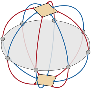
This scenario is schematized in figure 4. Each line of longitude (meridian) on the globe-like figure represents a branch connecting FP1 (top square) and FP1$^\prime$ (bottom square), like that shown in figure 3. The roll-merging half-branches are coloured in red and emerge from the corners of a square; the roll-disappearing half-branches in blue emerge from the sides of a square. The fact that four of each emerge at each of the squares corresponds to the fact that each of FP1 and FP1$^\prime$ contains four rolls and four inter-roll spaces that can undergo roll disappearance or roll merging. Each half-branch of one colour emanating from FP1 meets a half-branch of the opposite colour emanating from FP1$^\prime$ at the equator, which contains transcritical bifurcation points of different phases in $z$.

Figure 4. Schematic diagram of the set of FP4 branches associated with figure 3. The square on the top represents the pitchfork bifurcation point of FP1 (figure 3j), while the square on the bottom, rotated by $2{\rm \pi} /8$ with respect to the top one, represents that of FP1$^\prime$ (figure 3k). Four roll-merging half-branches, shown in red, emanate from four corners of each of the squares; and four roll-disappearing half-branches, shown in blue, emanate from four sides of each of the squares. These are the half-branches shown in figures 3( j,i,h,g,f) and 3(k,l,m,n,f), and also those obtained by $\tau (0,2.5)$, $\tau (0,5.0)$ and $\tau (0,7.5)$, in which the roll merging or disappearing occurs at other locations. Each roll-merging half-branch emanating from FP1 meets a roll-disappearing half-branch emanating from FP1$^\prime$, and vice versa, at the equator, on which are situated the transcritical bifurcation points with the FP2 branch, such as figure 3( f).

3.2.2. Eigenvectors of FP1 and FP1$^\prime$

Figures 3(b) and 3(c) show the unstable eigenmodes $e_3$ of FP1 and $e_4^\prime$ of FP1$^\prime$ at $Ra=13\,384$ that are responsible for the two simultaneous subcritical pitchfork bifurcations that create the two half-branches of FP4. We call these $e_3$ and $e_4^\prime$ because the FP1 (and FP1$^\prime$) branch at $Ra=13\,384$ has two larger positive eigenvalues resulting from the circle pitchfork bifurcation to FP3. Eigenvectors $e_3$ and $e_4^\prime$ have the same eigenvalue, $\lambda _{3,4}$. The Arnoldi method computes two linearly independent eigenmodes of the double eigenvalue $\lambda _{3,4}$; for $e_3$ we select the linear combination of these that most resembles the difference between FP4 and FP1 at the bifurcation point of figure 3( j). The eigenvectors of FP1$^\prime$ are related to those of FP1 by a translation $\tau (0,1.25)$. We select as $e_4^\prime$ the analogous combination of eigenmodes of FP1$^\prime$ that most resembles the difference between FP4 and FP1$^\prime$ at the bifurcation point of figure 3(k). Eigenmodes $e_3$ and $e_4^\prime$ differ qualitatively: $e_3$ has two narrow intense temperature extrema surrounded by wide diffuse patches of the opposite sign, while $e_4^\prime$ has two wide diffuse patches surrounded by narrow extrema. Each eigenmode has two centres of ${\rm \pi} _{xz}$ symmetry, at $z=2.5$ and $7.5$.

Examining the eigenvectors helps us to understand the progression from the fourfold translation-symmetric FP1 (and FP1$^\prime$) to FP4. The eigenvectors describe defects that, when added to FP1 (or FP1$^\prime$), lead to roll merging or roll disappearance. The red (hot) and blue (cold) diffuse patches of $e_3$ are in opposition to those of FP1 at the boundary between two rolls at $z=2.5$; compare figures 3(b) and 3( j). This implies that the between-roll boundary at $z=2.5$ becomes weaker along this half-branch. In contrast, at $z=7.5$, FP1 and $e_3$ have temperatures of the same sign, so this roll boundary is strengthened. Turning now to the pathway (k,l,m,n,f), this roll-disappearing half-branch is associated with eigenvector $e_4^\prime$ in figure 3(c). Eigenvector $e_4^\prime$ is very weak at $z=2.5$ and at $z=7.5$, around which rolls of FP1$^\prime$ are centred. However, the temperature of $e_4^\prime$ surrounding $z=2.5$ is such as to reinforce the roll at $z=2.5$ of FP1$^\prime$, whereas $e_4^\prime$ and FP1$^\prime$ display opposite temperatures surrounding $z=7.5$. The roll of FP1$^\prime$ at $z=7.5$ consequently disappears along this half-branch.

Eigenmodes of the Jacobian matrix describe the temporal dynamics near a fixed point $\bar {u}$, but we have used them above to describe the tangent along a branch (or half-branch) near a bifurcation. We now explain the justification for this. For a dynamical system ${\rm d}u/{\rm d}t=f(u,Ra)$, a curve of fixed points $\bar {u}(Ra)$ is defined via $0=f(\bar {u}(Ra),Ra)$. Differentiating in $Ra$ yields

(3.2)\begin{equation} 0=\frac{\partial f}{\partial Ra} + [{D}f]_{\bar{u}}\,\frac{{\rm d}\bar{u}}{{\rm d}Ra}, \end{equation}

where $[{D}f]_{\bar {u}}$ is the Jacobian evaluated at $\bar {u}$. Near a bifurcation, the Jacobian has an eigenvalue $\lambda _{bif}$ near zero so that multiplication by the inverse Jacobian projects onto the bifurcating eigenvector $e_{bif}$:

(3.3)\begin{equation} \frac{{\rm d}\bar{u}}{{\rm d}Ra}={-}[Df]_{\bar{u}}^{{-}1}\,\frac{\partial f}{\partial Ra} ={-}\sum_j \frac{1}{\lambda_j}\left\langle\frac{\partial f}{\partial Ra}, e_j\right\rangle e_j \approx{-}\frac{1}{\lambda_{bif}}\left\langle\frac{\partial f}{\partial Ra},e_{bif}\right\rangle e_{bif}, \end{equation}

where $\langle \cdot,\cdot \rangle$ is an inner product, and $(\lambda _j,e_j)$ are the eigenpairs of $[Df]_{\bar {u}}$, with $|1/\lambda _{bif}| \gg |1/\lambda _j|$ for the other eigenvalues of $[Df]_{\bar {u}}$. This leads to the expression

(3.4)\begin{equation} \bar{u}(Ra - \Delta Ra) \approx \bar{u}(Ra) - \Delta Ra\,\frac{{\rm d}\bar{u}}{{\rm d}Ra} \approx \bar{u}(Ra) +\frac{\Delta Ra}{\lambda_{bif}}\left\langle\frac{\partial f}{\partial Ra}, e_{bif}\right\rangle e_{bif} \end{equation}

for the evolution of a branch near a bifurcation.

3.2.3. Normal form of $D_4$ symmetry

The simultaneous occurrence of two pitchfork bifurcations described above is precisely the scenario seen in pattern formation on a square domain, which, like FP1 (and FP1$^\prime$), has the symmetry group $D_4$, generated by ${\rm \pi} _{xz}$ and $\tau (0,2.5)$. In the square, rolls can be oriented horizontally or vertically, and these are equivalent because they are related by a rotation by ${\rm \pi} /2$. The eigenvectors associated with vertical and horizontal rolls can also be combined to form diagonal eigenvectors. The nonlinear equations that are equivariant (compatible) with $D_4$ symmetry predict the existence of branches of diagonal states (Swift Reference Swift1985; Bergeon, Henry & Knobloch Reference Bergeon, Henry and Knobloch2001) that originate from eigenvectors that are equal superpositions of vertical and horizontal eigenmodes, as will be discussed below. The diagonal roll branches bifurcate simultaneously with the horizontal and vertical roll branches, but the nonlinear diagonal states are not related to the horizontal or vertical states by symmetry operations and are therefore not equivalent. Both types of branches have a reflection symmetry – vertical or horizontal in one case, and diagonal in the other case – so that their symmetry groups are $Z_2$.

This scenario for pattern formation on a square domain also exists for the FP1 branch, with the four co-rotating rolls playing the role of the four sides of a square, and the four inter-roll intervals playing the role of the corners. Instead of considering the FP4 branch with its endpoints FP1 and FP1$^\prime$ as we did in figure 3, we now consider a single phase of FP1 and its two bifurcations to roll-merging and roll-disappearing half-branches corresponding to its eigenvectors $e_3$ and $e_4$. Four bifurcating branches resembling figures 3( j)–3( f) result from eigenvector $e_3$ along with shifted and reflected versions, and four branches resembling figures 3(k)–3( f) result from $e_4$ along with shifted and reflected versions. The bifurcations occur at the same value of the Rayleigh number, but the branches are not equivalent, as seen in figures 2(a) and 3(a), for example, by the different locations of the saddle–node bifurcations emanating from FP1 and FP1$^\prime$.

We now give a more quantitative explanation of this scenario. Consider the dynamical system governing $(p,q)\in \mathcal {R}^2$:

(3.5a)$$\begin{gather} \dot{p} = (\mu - a p^2 - b q^2) p, \end{gather}$$

(3.5b)$$\begin{gather}\dot{q} = (\mu - b p^2 - a q^2) q, \end{gather}$$

with $\mu,a,b$ all real parameters. The bifurcation parameter is $\mu$, and $a,b$ are nonlinear coefficients that saturate the instability. System (3.5) is a projection of a larger system near a bifurcation onto the bifurcating eigenmodes. A normal form is the smallest system, in terms of both number of variables and polynomial order, that is able to reproduce the behaviour of the larger system near the bifurcation. The form of system (3.5) is dictated by the requirements that it be equivariant under (consistent with) change in sign of $p$ or $q$, and interchange of $p$ and $q$, which defines the group $D_4$.

The Jacobian of (3.5) is

(3.6)\begin{equation} \left[\begin{array}{cc} \mu -3ap^2 -bq^2 & -2bpq\\ -2bpq & \mu -bp^2 - 3aq^2 \end{array}\right]. \end{equation}

Evaluated at the trivial solution $(p,q)=(0,0)$, this becomes $\mu {\boldsymbol {I}}$, i.e. a double eigenvalue $\mu$. The non-trivial fixed points of system (3.5) are

(3.7a)$$\begin{gather} p ={\pm}\sqrt{\mu/a}, \quad q = 0, \end{gather}$$

(3.7b)$$\begin{gather}p = 0, \quad q={\pm}\sqrt{\mu/a}, \end{gather}$$

(3.7c)$$\begin{gather}p ={\pm}\sqrt{\mu/(a+b)}, \quad q ={\pm}\sqrt{\mu/(a+b)}, \end{gather}$$

(3.7d)$$\begin{gather}p ={\pm}\sqrt{\mu/(a+b)}, \quad q ={\mp}\sqrt{\mu/(a+b)}. \end{gather}$$

Thus (3.5) has eight non-trivial solutions, two each of types (3.7a), (3.7b), (3.7c) and (3.7d). Although solutions (3.7a) and (3.7b) are related to one another by the symmetry $(p,q) \rightarrow (-q,p)$, as are solutions (3.7c) and (3.7d), solutions (3.7c) and (3.7d) are not related to solutions (3.7a) and (3.7b) by interchanging $p$ and $q$, or by changing their signs.

The scenario by which FP1 gives rise to FP4 is analogous to system (3.5) and (3.7), with FP1 playing the role of the trivial solution $p=q=0$. The assumption of normal form theory is that FP4 solutions can be approximated as superpositions of the base state FP1 and its eigenvectors $e_3$ and $\tau (0,2.5)\,e_3$ at the bifurcation:

(3.8)\begin{equation} {\rm FP4} = {\rm FP1} + p(t)\,e_3 + q(t)\,\tau(0,2.5)\,e_3, \end{equation}

with $p(t)$ and $q(t)$ governed by the amplitude equations or normal form (3.5). The quantity $p$ measures the amplitude of eigenvector $e_3$ in figure 3(b), which gives rise to the half-branch in which two rolls merge at $z=2.5$. The phase-shifted $\tau (0,2.5)\,e_3$, whose amplitude is measured by $q$, gives rise to a different half-branch in which roll merging occurs at $z=5.0$. Figures 5(a,b) show these eigenvectors, while figure 5(c) shows their normalized sum. Further shifts, $\tau (0,5)\,e_3 = -e_3$ and $\tau (0,7.5)\,e_3 = -\tau (0,2.5)\,e_3$, correspond to $-p$ and $-q$, respectively.

Figure 5. (a) Eigenmode $e_3$ of FP1, with the same phase as in figure 3(b). (b) Quarter-domain-translated version of (a): $\tau (0,2.5)\,e_3$. (c) Superposition $(e_3+\tau(0,0.25)e_3)/\sqrt{2}$. (d) Superposition $(e_3-\tau (0,0.25) e_3)/\sqrt{2}$. Note that $(e_3+\tau (0,2.5)\,e_3)/\sqrt {2} = e_4= \tau (0,-3.75)\,e_4^\prime$ (compare with figure 3c).

Turning now to the four roll-disappearing half-branches bifurcating from FP1, these are produced by eigenvectors $\tau (0, 2.5 n)\,e_4$ for $n=0,1,2,3$. The normalized sum of the roll-merging eigenvectors $(e_3 + \tau (0, 2.5)\,e_3)/\sqrt {2}$ turns out to be the roll-disappearing eigenvector $e_4$, analogously to the fact that the sum of a $p$ solution and a $q$ solution yields a $p+q$ solution. (Because these are eigenvectors, their amplitudes have no importance.) The sum of two neighbouring roll-disappearing eigenvectors (not shown) is a roll-merging eigenvector, analogously to the combinations $(p+q)+(p-q)\propto p$ and $(p+q)-(p-q)\propto q$. This confirms the correspondence between the normal form (3.5) and our hydrodynamic system with its four-roll branch FP1, its connector branch FP4, and its eigenvectors $e_3$ and $e_4$.

3.2.4. Transcritical bifurcation between FP4 and $D_3$-symmetric FP2

Figure 3(a) shows the intersection between FP4 and the three-roll branch FP2 at figure 3( f) in a transcritical bifurcation (TC). From the point of view of FP2, the FP4 roll-merging half-branch ( j,i,h,g,f) can be called a roll-splitting half-branch when traversed in the opposite order ( f,g,h,i,j). Similarly, the FP4 roll-disappearing half-branch (k,l,m,n,f) can be called a roll-creation half-branch when traversed in the order ( f,n,m,l,k). Because FP2 has threefold translation symmetry $\tau (0,10/3)$, any of the three rolls in figure 3( f) can be the site of a roll-splitting or a roll-creation event, so six FP4 half-branches, three of each type, emanate from FP2 at TC. These join pairwise at FP2: for example, in figure 3, the upper half-branch with roll splitting at $z=2.5$ (figures 3h,i) meets the lower half-branch in which roll creation occurs at $z=7.5$ (figures 3m,l). (We assume that the saddle–node bifurcations have no effect on this scenario.)

The bifurcation from FP2 to FP4 breaks threefold translation symmetry but retains reflection symmetry ${\rm \pi} _{xz}$. This can be seen in figure 3(h), for example, where the roll centred at $z=2.5$ is stretched, while the other two rolls remain of the same size and related to one another by reflection in $z=2.5$. For figure 3(m), the reasoning is the same, but is applied to the inter-roll space at $z=7.5$.

We now turn to the eigenmodes of FP2 and FP4 close to TC. To the right of figure 3( f), figure 3(d) displays the eigenmode $e_5$ of FP2 at $Ra\gtrsim 11\,283$, leading to FP4. As previously, the name $e_5$ is used because FP2 has four eigenvalues with larger real parts. By a slight abuse of notation, we use $-e_5$ to denote the direction in which FP2 is approached from FP4 for $Ra\lesssim 11\,283$, and visualize it in figure 3(e). We obtain $\pm e_5$ by subtracting the temperature fields of FP2 from FP4 states to the right and left of point ( f) in figure 3(a), as well as from the Arnoldi method. Using (3.4) again, we can superpose FP2 in figure 3( f) with eigenvector $e_5$ in figure 3(d) to yield FP4 in figures 3(g) and 3(h), since $e_5$ opposes the roll in FP4 centred at $z=2.5$, leading to an expanded roll and eventually to roll splitting. Similarly, we can superpose figure 3( f) with eigenvector $-e_5$ in figure 3(e) to yield FP4 in figures 3(n) and 3(m). Since $-e_5$ opposes the rolls on either side of $z=7.5$ in FP4, this inter-roll space expands, eventually making room for roll creation.

As FP2 has threefold translation symmetry, $e_5$ of FP2 can be shifted by $\pm 10/3$ in $z$, yielding a triple of eigenvectors only two of which are linearly independent, since $\tau (0,10/3)\,e_5 + \tau (0,-10/3)\,e_5 = -e_5$. These share the same eigenvalue $\lambda _{5,6}$, depicted in figure 6(a). Along branch FP4, these eigenvectors are modified, so that they are no longer related by $\tau (0,\pm 10/3)$ and hence have different eigenvalues, shown as $\lambda _5$ and $\lambda _6$ in figure 6(b). Eigenvectors $e_5$ and $e_6$ of FP4 at $Ra=11\,292.2$, shown in figures 6(d) and 6(e), are symmetric and anti-symmetric, respectively, with respect to $xz$-reflection symmetry about $z=2.5$ and $z=7.5$.

Figure 6. (a,b) Evolution of eigenvalues relevant to transcritical bifurcation ${\rm FP2}\leftrightarrow {\rm FP}4$ at $Ra=11\,283$: (a) bifurcating double eigenvalue $\lambda _{5,6}$ of FP2; (b) two eigenvalues of FP4, $\lambda _5$ (whose sign is reversed with respect to $\lambda _{5,6}$ of FP2) and $\lambda _6$, where $|\lambda _6| \approx 3\,|\lambda _5|$. (c) Base state FP4 for eigenmodes $e_5$ and $e_6$ in (d,e). (d,e) Eigenmodes $e_5$ and $e_6$ of FP4 associated with $\lambda _5$ and $\lambda _6$ at $Ra=11\,292.2$ (red circles in b). Eigenmode $e_5$ is $xz$-reflection symmetric about $z=2.5$ (and $z=7.5$), and is related to a change in amplitude along the branch, while $e_6$ is anti-$xz$-reflection symmetric about $z=2.5$ (and $z=7.5$), and is related to a change in phase perpendicular to the branch. In (c), the same colour bar is used as in figures 2 and 3.

3.2.5. $D_3$ symmetry

We now consider the equations governing bifurcation in the presence of $D_3$ symmetry. In this case, we will consider not the normal form, but a related system, i.e. the universal unfolding of the degenerate case of the normal form, because these are the equations that best describe our results. See Gambaudo (Reference Gambaudo1985), Golubitsky et al. (Reference Golubitsky, Stewart and Schaeffer1988) and Dawes (Reference Dawes2005) for details. These equations are

(3.9a)$$\begin{gather} \dot{p} ={-}\mu p + b(p^2-q^2) - ap(p^2+q^2), \end{gather}$$

(3.9b)$$\begin{gather}\dot{q} ={-}\mu q - 2bpq - aq(p^2+q^2), \end{gather}$$

with $a, b$ real parameters, $\mu$ the bifurcation parameter, and $(p,q)$ the amplitudes of eigenmodes of the FP2 branch. As stated in § 3.2.3, the correspondence of (3.9) with our high-dimensional hydrodynamic system consists of approximating FP4 by a superposition of FP2 with its eigenvectors $e_5$ and $\tau (0, 10/3)\,e_5$ at the bifurcation point, whose amplitudes are represented here by $p$ and $q$:

(3.10)\begin{equation} {\rm FP4} = {\rm FP2} + p(t)\,e_5 + q(t)\,\tau(0, 10/3)\,e_5. \end{equation}

Let us begin by studying steady solutions with $q=0$:

(3.11a)$$\begin{gather} p= 0, \end{gather}$$

(3.11b)$$\begin{gather}\mu - bp + ap^2 = 0 \Rightarrow p =\left[b \pm \sqrt{b^2 - 4\mu a}\right]/(2a). \end{gather}$$

These are shown in figure 7(a). The trivial solution $p=0$ corresponds to the FP2 branch. Two sets of solutions corresponding to FP4 are created at $\mu =b^2/(4a)$; this is a saddle–node bifurcation. The set of solutions closer to zero intersects the trivial FP2-type branch $p=0$ in a transcritical bifurcation at $\mu =0$. These two bifurcations are marked as SN and TC in the parabola in figure 7(a). The saddle–node and transcritical bifurcations are also seen in the hydrodynamic case and are labelled by (g,f) in the bifurcation diagram of figure 3.

Figure 7. (a) Parabola in the $\mu \unicode{x2013}p$ plane representing the FP4-like solutions of $\mu - bp + ap^2=0$ (with $a,b$ positive) of (3.9). The thicker horizontal axis ($p=0$) represents the FP2 branch. The saddle–node SN at $\mu =b^2/(4a)$ and transcritical bifurcation TC at $\mu =0$ are marked by dots. The region surrounded by the grey square corresponds to the meeting point of two types of half-branches (red and blue) and to the double-cone schematic in (b). (b) Three-dimensional schematic figure in the $p\unicode{x2013}q\unicode{x2013}\mu$ plane illustrating the solutions near TC. Each cone contains three FP4 solutions of each type (red or blue), with angular (phase) separation $2{\rm \pi} /3$. These all intersect the $\mu$ axis representing FP2 at $\mu =0$ in a transcritical bifurcation. The solid thicker line (red on the left cone, blue on the right) represents the path of figure 3, while the five dashed lines correspond to paths that would be observed with a $\Delta z=\pm 10/3$ shift in $z$ or a reversal of the path direction, or both.

The Jacobian of (3.9) is

(3.12)\begin{equation} \left[\begin{array}{@{}cc@{}} -\mu + 2bp - 3ap^2 - aq^2 & -2bq -2apq\\ -2bq -2apq & -\mu - 2bp - 3aq^2 - ap^2 \end{array}\right]. \end{equation}

Evaluated at $(p,q)=(0,0)$ corresponding to FP2, this becomes $-\mu {\boldsymbol {I}}$, i.e. one double eigenvalue $-\mu$. Evaluated at the $q=0$, $\mu - bp+ ap^2=0$ solution corresponding to FP4, we obtain

(3.13)\begin{equation} \left[\begin{array}{@{}cc@{}} -\mu + 2bp - 3(bp-\mu) & 0 \\ 0 & -\mu - 2bp +(\mu-bp) \end{array}\right] = \left[\begin{array}{@{}cc@{}} 2\mu - bp & 0 \\ 0 & -3bp \end{array}\right]. \end{equation}

Since $ap^2$ can be neglected near TC, the FP4-type solutions (3.11b) take the form $p\approx \mu /b$. (In accordance with the previous nomenclature, these are two half-branches, one for $\mu >0$, and the other for $\mu <0$.) The Jacobian becomes

(3.14)\begin{equation} \left[\begin{array}{@{}cc@{}} 2\mu - \mu & 0 \\ 0 & -3\mu \end{array}\right] = \left[\begin{array}{@{}rc@{}} \mu & 0 \\ 0 & -3\mu \end{array}\right]. \end{equation}

Thus the FP4 states emanating from TC each have two eigenvalues of opposite signs, which are approximately $\mu$ (in the $p$ direction connecting FP2 and FP4) and $-3\mu$ (in the $q$ direction, perpendicular to $p$). This is precisely the behaviour seen in figures 6(a) and 6(b). Indeed, if we define $-\mu$ to be the eigenvalue of FP2 in figure 6(a), then we find that the eigenvalues of FP4 in figure 6(b) are approximately $\mu$ and $-3\mu$.

Dropping now the requirement that $q=0$, two more solutions to (3.9) of FP4-type exist, related to the $q=0$ solution by rotation by $\pm 2{\rm \pi} /3$ in the $p\unicode{x2013}q$ plane:

(3.15)\begin{equation} \left(\begin{array}{@{}c@{}} p \\ q \end{array}\right) \rightarrow \left(\begin{array}{@{}rr@{}} \cos(2{\rm \pi}/3) & \pm \sin(2{\rm \pi}/3) \\ \mp \sin(2{\rm \pi}/3) & \cos(2{\rm \pi}/3) \end{array}\right) \left(\begin{array}{@{}c@{}} p\\q \end{array}\right). \end{equation}

Each can be assigned an amplitude $\sqrt {p^2+q^2} \approx \mu /b$ and a phase $\tan ^{-1}(q/p)$. The phase can in turn be mapped to a vertical location in $[0,L_z)$ of a defect in one of the three rolls or inter-roll spaces. Such a defect is a precursor to roll splitting or roll creation, respectively, as one leaves TC along one of the half-branches. The eigenvalues of the other two FP4 solutions are again $\mu$ and $-3\mu$. The eigenvector associated with $\mu$ resembles the defect itself; i.e. it corresponds to a change in its amplitude. The eigenvector associated with $-3\mu$ corresponds to a change in phase, i.e. a tendency for the defect to translate in $z$. Like all eigenvectors, this tendency is local to TC, and nonlinear trajectories deviate from the phase-translation path before any phase change is actually achieved.

A schematic illustration of these solutions and the transcritical bifurcation is shown in figure 7(b). Roll-splitting and roll-creation half-branches are shown in red and blue, respectively. Three of each type of half-branch exist on each cone. The thick red and blue half-branches comprise the branch followed in figure 3 from FP1 to FP1$^\prime$, along which roll merging and then roll creation occur. Another two half-branches comprise a branch from FP1 to FP1$^\prime$ along which roll disappearance and then roll splitting occur. The other four branches have starting or ending points that are shifted by $\Delta z\pm 10/3$ from FP1 or FP1$^\prime$. These six branches are all included in figure 7(b) in order to give a full picture of the transcritical bifurcation; their depiction is not necessary for the understanding of the single path of figure 3.

3.3. Wider perspectives

In the previous subsections, we have extensively discussed the $D_4$ and $D_3$ bifurcation scenarios separately. We now take a wider perspective, discussing various aspects of the interaction between the $D_4$ and $D_3$ bifurcations.

The double-cone visualization of figure 7 may seem incompatible with the globe-like visualization of figure 4. In fact, each figure is local, and the two visualizations have only two branches in common. Each branch belongs simultaneously to a sphere and to a double cone. Four of the branches traversing TC through the double cone are not present in figure 4; two more spheres would be required to contain them. Similarly, more double cones would be required to contain all the meridians of the globe. A total of $2 \times 3 \times 8 = 48\text { half-branches} = 24\text { branches}$ are necessary to close the system, i.e. to include all branches that emanate from all bifurcations encountered by branches created at FP1. (Other phase changes in $z$ lead to a continuous infinity of branches.) It is not possible (or we have not been able) to depict the entire scenario in a single diagram. However, we again emphasize that figure 3 can be understood without recourse to this large number of other symmetry-related branches.

We have depicted FP4 as connecting two versions of FP1 related by a shift $\Delta z=1.25$, while passing continuously through a transcritical bifurcation at FP2. However, there exists another construction of this scenario: the transcritical bifurcation could be broken apart in such a way that rather than traversing FP2 smoothly, FP4 enters the transcritical bifurcation at FP2 but then exits at FP2$^\prime \equiv \tau (1.25,0)$ FP2. In figure 3, the second row would contain not a repeated version of figure 3( f), but instead a shifted version of it. Figures 3(n,m,l,k) would then also be shifted, with the result that figure 3(k) would be identical to figure 3( j) instead of being a shifted version of it. In the schematic figure 7, the left cone and right cone would each be reflected in such a way as to separate the two vertices and to join the two bases. In the schematic figure 4, the equator would be cut open, while the north pole and a rotated south pole would be joined. In summary, the FP4 branches start and end in states with a shift $\Delta z=1.25$ between them, but this can happen either by connecting FP1 and FP1$^\prime$ while passing continuously through FP2, as discussed in §§ 3.2.1–3.2.5, or alternatively, by connecting FP2 and FP2$^\prime$ while passing continuously through FP1. Yet another alternative point of view is to double the FP4 branch, passing continuously through FP1, FP2, FP1$^\prime$, FP2$^{\prime }$, FP1 without any phase jumps.

Dangelmayr (Reference Dangelmayr1986) determined the normal form for the occurrence of bifurcations to periodic patterns of two different wavenumbers, and its unfolding. The equations for the $D_3$–$D_4$ mode interaction predict a number of the features that we observe for our branch FP4 connecting the four-roll and three-roll branches FP1 and FP2, such as the existence of two qualitatively different connecting branches (like our roll-disappearing and roll-merging branches), a nearby saddle–node bifurcation on one of them (like that of figure 3g), and a Hopf bifurcation giving rise to temporally periodic solutions (such as the PO1 branch to be discussed in § 4.2). Some of the features of our scenario are not present in the normal form, in particular the subcriticality of the bifurcations from FP1 to FP4 and the possibly related two additional saddle–node bifurcations of FP4. Another feature that is not mentioned in Dangelmayr (Reference Dangelmayr1986) is the involvement of the two $L_z/8$ phase-shifted versions of FP1. The normal form predicts the stable and unstable eigenvalues of the solution branches, such as those discussed in the next subsection.

3.4. Stability

We start by discussing the stability of the FP4 state, which changes multiple times along its branch. Bifurcating subcritically from FP1, the upper (roll-merging) branch of FP4 is initially unstable and inherits the four unstable eigendirections of FP1 at $Ra=13\,383.9$ (two of which are the $y$-dependent modes that give rise to FP3). Three of these four positive eigenvalues are successively stabilized along the upper branch by undergoing tertiary bifurcations to quaternary states that are not discussed in this work. The last positive eigenvalue is stabilized after undergoing a saddle–node bifurcation at $Ra=8255$. This stability is short-lived, however, ending when FP4 undergoes a Hopf bifurcation at $Ra=9980$ to a periodic orbit to be discussed in the next section. The FP4 branch undergoes two more saddle–node bifurcations, at $Ra=11\,437$ and then at $Ra=10\,020$, before it finally terminates on FP1$^\prime$, a translated version of the FP1 branch that also has four unstable eigendirections. The connector branch FP4 is thus stable over the interval $8255< Ra<9980$, along with the four-roll branch FP1. However, it is not surprising that the FP4 branch was overlooked by Gao et al. (Reference Gao, Sergent, Podvin, Xin, Le Quéré and Tuckerman2013), since it is unstable over most of its range of existence, and its bifurcation occurs from a point at which FP1 is unstable.

As mentioned in § 3.1, in domain $[L_x, L_y, L_z] = [1, 1, 10]$, branch FP1 is stable at onset, while FP2 is unstable. Both FP1 and FP2 exist in domain $[1, 0, 10]$ as well. After the bifurcation to FP1, the conductive state acquires two unstable $y$-independent eigenmodes. These are inherited by FP2 at onset, and so FP2 is also unstable when computed in domain $[1, 0, 10]$. Concerning the stability of FP1, since the bifurcation to FP3 breaks $y$-translation symmetry, it does not occur in domain $[1,0,10]$, and FP1 remains stable until the bifurcation to FP4 (in § 3.2) at $Ra=13\,383.9$. Regarding FP4, its range of stability does not change if computed in domain $[1,0,10]$, since the unstable part of the FP4 branch always has at least one unstable $y$-independent eigenmode. Due to their fourfold symmetry, FP1 and FP3 can exist in domain $[1, 1, 2.5]$, in which their existence and stability ranges are the same as in $[1, 1, 10]$. These ranges are summarized and compared in table 1 below. Since every zero-crossing of an eigenvalue or of its real part is accompanied by a bifurcation, there necessarily exist many more branches that we have not computed, for example along the FP4 branch.

Table 1. Summary of bifurcation sequence and comparison with the literature, including all fixed points (FP) and periodic orbits (PO) mentioned in this paper. All of the states exist in domain $[L_x, L_y, L_z] = [1, 1, 10]$, while only some exist in smaller domains $[1, 1, 2.5]$ and $[1, 0, 10]$. For each of the three domains, we summarize the ranges of existence and stability for all states that we have computed. States existing in two domains may be stable in the smaller domain but unstable in the larger domain. When upper limits are listed as 14 000 or 13 300, these numbers are not the end of the branch, but where we stopped the numerical continuation. The Rayleigh number ranges given in the last column correspond to those reported by Gao et al. (Reference Gao, Sergent, Podvin, Xin, Le Quéré and Tuckerman2013, Reference Gao, Podvin, Sergent and Xin2015) and do not necessarily strictly correspond to existence or stability ranges. Ranges not reported are indicated by ‘—’.

4.1. Period-doubling cascade: PO3–PO6

Periodic orbit PO3 arises from FP3 in a supercritical Hopf bifurcation at $Ra=11\,261$, at which all of the spatial symmetries of FP3 are preserved. This is depicted in the upper left inset of figure 8(a), where the two red branches bifurcating from the FP3 branch correspond to the maximum and minimum of $\| \theta \|_2$ along PO3. Orbit PO3 was observed by Gao et al. (Reference Gao, Sergent, Podvin, Xin, Le Quéré and Tuckerman2013, Reference Gao, Podvin, Sergent and Xin2015), and the threshold that they reported is $Ra=11\,270$. Comparing the vorticity isosurfaces of FP3 at $Ra = 11\,000$ and PO3 at $Ra = 11\,500$, Gao et al. (Reference Gao, Sergent, Podvin, Xin, Le Quéré and Tuckerman2013) show in their figures 10 and 13 that PO3 conserves most of the spatial structure of FP3, with the addition of strands connecting the rolls that appear and disappear periodically.

Orbit PO3 undergoes a period-doubling bifurcation leading to PO4 at $Ra = 12\,066$, with further period-doubling bifurcations leading to PO5 and PO6 at $Ra=12\,257$ and 12 306 (very similar to the thresholds $Ra=12\,068$, 12 258 and 12 306 found by Gao et al. Reference Gao, Podvin, Sergent and Xin2015). The temperature norms $\| \theta \|_2$ of PO3–PO6 are all close, as is typical for period-doubling cascades. The periods of these limit cycles are shown in figure 8(b), where period-doubling bifurcation points are indicated by stars. We were able to continue all of PO3–PO6 until at least $Ra=13\,300$. The dynamics of PO4–PO6 are very similar to those of PO3, so we do not show visualizations of them. Orbits PO3–PO6 inherit the fourfold symmetry $[D_4]_{xz}$ of FP3, hence their spatial and temporal variations all take place within a single roll. These states and the transitions between them are the only phenomena that we report that are not related to competition between three and four rolls.

We refer readers to Gao et al. (Reference Gao, Podvin, Sergent and Xin2015) for their measurements of the convergence to the Feigenbaum number characterizing the accumulation of period-doubling bifurcations until chaos. Indeed, Gao et al. (Reference Gao, Sergent, Podvin, Xin, Le Quéré and Tuckerman2013) observed that the flow in $[L_x, L_y, L_z] = [1, 1, 10]$ becomes irregular following subharmonic oscillations at $Ra=12\,200$. Gao et al. (Reference Gao, Podvin, Sergent and Xin2015) estimated that a chaotic regime is reached at approximately $Ra = 12\,320$ (in $[L_x, L_y, L_z] = [1, 1, 2.5]$), and our DNS results confirm this. Gao et al. (Reference Gao, Podvin, Sergent and Xin2015) also discovered and reported five other periodic windows in their table II, each corresponding to another period-doubling cascade leading to chaotic behaviour. Although we have converged and continued these periodic windows, we omit them from the bifurcation diagram to avoid its becoming even more crowded.

Domain size has a major effect on the stability of PO3–PO6. When computed in a domain of the size of one wavelength $[1, 1, 2.5]$, PO3 is stable until it is succeeded by PO4, but in the domain $[1, 1, 10]$, it becomes unstable at $Ra\approx 11\,700$ by undergoing a large-wavelength instability which breaks the fourfold symmetry. Since this is prior to the period-doubling bifurcation, PO4, PO5, PO6 and the subsequent states resulting from the period-doubling cascade are also unstable in $[1, 1, 10]$. The stability properties that we have chosen to indicate in figure 8(a) for PO3–PO6 are those for the domain $[1, 1, 2.5]$. We have summarized the range of existence and stability of PO3–PO6 in both three-dimensional domains in table 1. Because FP3 is a three-dimensional state, PO3–PO6 do not exist in the two-dimensional domain $[1, 0, 10]$.

4.2. Wavelength-changing periodic orbits: PO1 and PO2

For $Ra>12\,200$ in domain $[1, 1, 10]$, Gao et al. (Reference Gao, Sergent, Podvin, Xin, Le Quéré and Tuckerman2013) observed that numerical simulations started from a random initial condition settled down to three rolls, while four rolls were found intermittently. They also observed hysteresis in a simulation at $Ra=12\,000$, initiated from an instantaneous three-roll flow field at $Ra = 12\,200$, which finally settled down to a periodic orbit with three rolls. We have carried out DNS at nearly the same parameter values, illustrated in figure 9(a), which show long intervals of two types of time-periodic behaviour, which we call PO1 and PO2. The simulation is started from a random initial condition. The initial chaotic behaviour for $t \lesssim 250$ is succeeded by the weakly unstable PO1 ($300 \lesssim t \lesssim 650$). Afterwards, PO2 is visited ($1000 \lesssim t \lesssim 1600$) before a transition via subcritical period-doubling to a fully chaotic state ($t \gtrsim 1800$), which then persists without relaminarization. A phase portrait of these DNS is shown in figure 9(b), where instantaneous flow fields are represented by grey dots in the $D/I\unicode{x2013}I$ plane, where $D$ is the dissipation due to viscosity, and $I$ is the thermal energy input due to buoyancy. It can be seen that the two periodic orbits, with relatively low input/dissipation, are surrounded by the fully chaotic dynamics in this projection.

Figure 9. The DNS at $Ra=12\,200$. (a) Time series initialized by random initial conditions. The trajectory passes through two unstable time-periodic flows emphasized in the inset, PO1 ($300< t<650$) with period $T=27.6$, and PO2 ($1000< t<1600$) with period $T=34.5$. (b) Projection of the instantaneous flow fields, separated by $\Delta t=1$, of the chaotic dynamics and of the two periodic orbits onto the thermal energy input ($I$) and the viscous dissipation over energy input ($D/I$). (c–e) Flow structures of PO1 visualized via the temperature field on the $y$–$z$ plane (at $x=0$) and $x$–$z$ plane (at $y=0.5$). During the cycle, the longest of the three rolls lengthens and begins to fragment, and then recovers. The flow structures of PO2 are shown in figure 11.

Continuing PO1 backwards in Rayleigh number, we find that PO1 is created via a supercritical reflection-symmetry-breaking Hopf bifurcation from FP4 at $Ra=9980$, where FP4 is stable, so that PO1 is stable at onset. The complex conjugate neutral eigenvector pair of FP4 is anti-$xz$-reflection symmetric, so PO1 has the spatial symmetry group $S_{PO_1} \equiv \langle {{\rm \pi} _y, \tau (\Delta y,0)} \rangle \sim [O(2)]_y$, and the spatio-temporal symmetry

(4.1)\begin{equation} (u,v,w,\theta)(x,y,z_0+z,t+T/2) = ({-}u,v,-w,-\theta)({-}x,y,z_0-z,t), \end{equation}

where here, $z_0 \approx 4$ and $T/2 \approx 14$; compare figures 9(d) and 9(e), as well as figure 10(a).

Figure 10. Temperature profile $\theta _{local}$ at fixed $x, y$ and along $z\in [0,10]$ for two instants of (a) PO1, period $T=27.6$, and (b) PO2, period $T=34.5$, at $Ra=12\,200$. The time interval between two instants for both PO1 and PO2 is approximately half of the corresponding period. For PO1 in (a), the same $x$ and $y$ locations are used, while for PO2 in (b), the $y$-locations at which the measurements are taken differ by $L_y/2$. The instantaneous temperature fields at $t=12$ and $t=26$ for PO1 as well as at $t=6$ and $t=23$ for PO2 are shown in figures 9 and 11.

Orbit PO1 arises from FP4 at a Rayleigh number at which it has three unequal rolls; its temporal dynamics consists of periodic lengthening and near-fragmentation of the longest roll. Figure 10 shows temperature profiles in $z$ for PO1 (and PO2) at fixed $x$ and $y$ locations, and at two instants separated in time by approximately a half-period. In these profiles, two successive zero-crossings ($\theta _{local}(z)=0$) correspond to one roll. Figure 10(a) shows a close, but unsuccessful approach to roll creation in PO1 at $z\approx 3$ ($t=12$) and then again at $z\approx 5$ ($t=26$).

Orbit PO1 loses stability in a supercritical pitchfork bifurcation at $Ra=12\,013$ (emphasized in the upper right inset of figure 8a), leading to the creation of PO2, in which $y$-translation symmetry is broken, but $y$-reflection symmetry is retained: $S_{PO_2} \equiv \langle {{\rm \pi} _y} \rangle \sim [Z_2]_y$. Unlike PO1, in PO2 the central roll succeeds in splitting, as can be seen in figures 11(b) and 11(h), as well as by the zero-crossings in figure 10(b), but only temporarily (figures 11(b,e,h,k). Orbit PO2 has the spatio-temporal symmetry

(4.2)\begin{equation} (u,v,w,\theta)(x,y,z_0+z,t+T/2) = ({-}u,v,-w,-\theta)({-}x,y+0.5,z_0-z,t), \end{equation}

where $z_0 \approx 4$ and $T/2 \approx 17$. (The wavy structure of PO2 leads to the requirement that a half-domain shift in $y$ be included in (4.2). The combination of $\tau (0.5,0)$ and ${\rm \pi} _{xz}$ relates the red upward-facing ‘tongues’ centred at $y=0.5$ to the blue downward-facing ‘tongues’ centred at $y=0$.)

Figure 11. Three-dimensional periodic orbit PO2 at $Ra=12\,200$ (with period $T=34.5$) via two complementary visualizations of the temperature field: (a–f) $y$–$z$ plane at $x=0$, and (g–l) $x$–$z$ plane at $y=0.5$.

Orbit PO2 undergoes a saddle–node bifurcation at $Ra=12\,832$, and we followed this PO2 branch until $Ra=12\,804$, shortly after the saddle–node bifurcation. Also, PO2 undergoes a secondary Hopf bifurcation (also called a Neimark–Sacker or torus bifurcation) at $Ra=12\,082$, at which a complex conjugate pair of eigenvalues crosses the real axis, which generally leads to a torus that we will not discuss in the present work. Thus PO2 is stable only over a very small range of Rayleigh number ($12\,013 < Ra < 12\,082$), as can be seen in the upper right inset of figure 8(a). It is therefore not surprising that PO2 was not observed by Gao et al. (Reference Gao, Sergent, Podvin, Xin, Le Quéré and Tuckerman2013). The period of PO1 remains nearly constant over a wide range of $Ra$, while that of PO2 increases with $Ra$ and then stays almost constant.

Orbits PO1 and PO2 capture the oscillatory dynamics of convection rolls. Orbit PO1 has three non-uniform rolls of fluctuating size and intensity (figures 9c–e). Although some rolls stretch and become quite weak, they never actually split anywhere along the branch. For PO2, the number of rolls varies between three (figures 11(a,c,d,f) along with figures 11(g,i,j,l)) and four (figures 11(b,e) along with figures 11(h,k)). We suggest that the intermittency and hysteresis observed by Gao et al. (Reference Gao, Sergent, Podvin, Xin, Le Quéré and Tuckerman2013) are a manifestation of visits to the coexisting unstable periodic orbits PO1 and PO2.

Since PO1 is $y$-independent, it can also exist in domain $[L_x, L_y, L_z] = [1, 0, 10]$. While the existence ranges of PO1 in domains $[1, 0, 10]$ and $[1, 1, 10]$ are the same, their stabilities differ: in $[1, 0, 10]$, the bifurcation to $y$-dependent PO2 does not occur, so PO1 remains linearly stable at least until $Ra=14\,000$, the upper limit at which we stopped the continuation. Gao et al. (Reference Gao, Sergent, Podvin, Xin, Le Quéré and Tuckerman2013) also observed this oscillating three-roll flow in the two-dimensional domain $[1, 0, 10]$, for $13\,500< Ra<15\,300$. Orbits PO1 and PO2 cannot exist in domain $[1,1,2.5]$, and PO2 cannot exist in domain $[1,0,10]$. The existence and stability intervals that we have computed for all of these flows are stated and compared with those of Gao et al. (Reference Gao, Sergent, Podvin, Xin, Le Quéré and Tuckerman2013, Reference Gao, Podvin, Sergent and Xin2015) in table 1.