


1. Introduction
Thermal convection influenced by rotation has been extensively studied to understand key aspects of fluid dynamics in many geophysical and astrophysical contexts (e.g. Chandrasekhar Reference Chandrasekhar1961; Glatzmaier Reference Glatzmaier2013; Zhang & Liao Reference Zhang and Liao2017; Ecke & Shishkina Reference Ecke and Shishkina2023). These include the circulation patterns within planetary atmospheres (e.g. Mitchell et al. Reference Mitchell, Scott, Seviour, Thomson, Waugh, Teanby and Ball2021) and the motions in the interiors of planets (e.g. Heimpel, Aurnou & Wicht Reference Heimpel, Aurnou and Wicht2005; Aurnou et al. Reference Aurnou, Calkins, Cheng, Julien, King, Nieves, Soderlund and Stellmach2015) and stars (e.g. Miesch Reference Miesch2005). Rotating convection has been studied in the linear regime, where the onset may be steady or oscillatory, and in the nonlinear regime, where motions may be laminar or turbulent, and has been investigated in different geometries, such as planar, spherical and cylindrical domains, thus making it a rich subject. Our focus here is on plane-layer, steady, Boussinesq, linear convection in a rapidly rotating system.
Mechanical and thermal boundary conditions play an important role in our ability to apply simplified models to real-world scenarios (e.g. Sakuraba & Roberts Reference Sakuraba and Roberts2009; Long et al. Reference Long, Mound, Davies and Tobias2020). In studies of convection, two limiting cases for thermal boundary conditions are frequently examined: (i) ‘perfectly conducting’ or fixed-temperature boundary conditions, where the temperature remains constant along the bounding surfaces; and (ii) ‘perfectly insulating’ or fixed-flux boundary conditions, where (for uniform thermal conductivity) the normal derivative of temperature is fixed at the boundaries. Thermal boundary conditions relevant to geophysical and astrophysical contexts often fall within the spectrum between these fixed-flux and fixed-temperature extremes. Comprehending the dynamics at these two extremes is therefore crucial to advancing our understanding of geophysical and astrophysical systems.
Rotating Rayleigh–Bénard convection (RRBC) is the study of thermal convection in a horizontal fluid layer heated from below while the entire system is rotated about the vertical axis, thereby combining buoyancy-driven and rotational effects. For Boussinesq, linear RRBC under rapid rotation, the case with impermeable, stress-free and fixed-temperature boundaries is notable as it can be solved analytically (e.g. Chandrasekhar Reference Chandrasekhar1961). The case with fixed-flux boundaries presents greater complexity as the eigenfunctions are no longer simple trigonometric functions. However, since under the constraint of rapid rotation the balance between Coriolis, buoyancy and viscous terms leads to a very small preferred horizontal length scale, the solution in the bulk of the fluid is independent of the choice of boundary conditions. Thus different mechanical and thermal boundary conditions can be explored through perturbative methods; this enables analytical progress beyond the impermeable, stress-free and fixed-temperature case. Exploiting this property, we derive asymptotic solutions for the linear onset of steady, Boussinesq RRBC under rapid rotation with impermeable, stress-free, fixed-flux boundary conditions.
In the absence of rotation, the most readily destabilised mode of linear Rayleigh–Bénard convection with impermeable, stress-free, fixed-temperature boundaries has a finite wavenumber (Chandrasekhar Reference Chandrasekhar1961). In contrast, for fixed-flux boundary conditions, the wavenumber of the most readily destabilised mode is zero, imposing large aspect ratio cells at onset (Hurle, Jakeman & Pike Reference Hurle, Jakeman and Pike1967). Chapman & Proctor (Reference Chapman and Proctor1980) considered the evolution of long but finite wavelength perturbations in the nonlinear regime, showing that steady solutions favour the growth of the longest possible wavelength in large domains. These wide cells continue to dominate at high Rayleigh number (Hewitt, Mckenzie & Weiss Reference Hewitt, McKenzie and Weiss1980), where the Rayleigh number $ Ra$
is a dimensionless measure of the thermal driving. Johnston & Doering (Reference Johnston and Doering2009) showed using two-dimensional numerical simulations that the heat transport of the fixed-temperature and fixed-flux systems converge at
$ Ra$
is a dimensionless measure of the thermal driving. Johnston & Doering (Reference Johnston and Doering2009) showed using two-dimensional numerical simulations that the heat transport of the fixed-temperature and fixed-flux systems converge at $ Ra\approx 5\times 10^6$
for
$ Ra\approx 5\times 10^6$
for $ Pr=1$
, where the Prandtl number
$ Pr=1$
, where the Prandtl number $ Pr$
is the ratio of thermal diffusivity to kinematic viscosity, and the flow becomes turbulent. For three-dimensional simulations, the heat transport for both cases also become equal, but at a higher value of
$ Pr$
is the ratio of thermal diffusivity to kinematic viscosity, and the flow becomes turbulent. For three-dimensional simulations, the heat transport for both cases also become equal, but at a higher value of $ Ra$
(Stevens, Lohse & Verzicco Reference Stevens, Lohse and Verzicco2011).
$ Ra$
(Stevens, Lohse & Verzicco Reference Stevens, Lohse and Verzicco2011).
The onset of linear RRBC with impermeable, stress-free and fixed-flux boundaries has been studied by Dowling (Reference Dowling1988), who determined the rotational strength required for the critical wavenumber $k^c$
to become non-zero. For
$k^c$
to become non-zero. For $0 \leqslant \textit{Ta} \lt 97.4$
, where
$0 \leqslant \textit{Ta} \lt 97.4$
, where $ \textit{Ta}$
is the Taylor number, a non-dimensional measure of the rotation rate, the onset of convection is steady with
$ \textit{Ta}$
is the Taylor number, a non-dimensional measure of the rotation rate, the onset of convection is steady with $k^c = 0$
. For
$k^c = 0$
. For $97.4 \lt \textit{Ta} \lt 180.15$
, either stationary convection with
$97.4 \lt \textit{Ta} \lt 180.15$
, either stationary convection with $k^c = 0$
or overstability with
$k^c = 0$
or overstability with $k^c\neq 0$
occurs at onset, depending on
$k^c\neq 0$
occurs at onset, depending on $ Pr$
. For
$ Pr$
. For $ \textit{Ta} \gt 180.15$
, the system can favour steady or oscillatory convection, both with
$ \textit{Ta} \gt 180.15$
, the system can favour steady or oscillatory convection, both with $k^c \gt 0$
. Takehiro et al. (Reference Takehiro, Ishiwatari, Nakajima and Hayashi2002) investigated both the weakly rotating and rapidly rotating linear systems with stress-free and fixed-flux boundary conditions at the onset of convection. Using a modal truncation approach, they demonstrated that as
$k^c \gt 0$
. Takehiro et al. (Reference Takehiro, Ishiwatari, Nakajima and Hayashi2002) investigated both the weakly rotating and rapidly rotating linear systems with stress-free and fixed-flux boundary conditions at the onset of convection. Using a modal truncation approach, they demonstrated that as $ \textit{Ta} \to \infty$
, the critical Rayleigh number and wavenumber for both types of thermal boundary conditions converge.
$ \textit{Ta} \to \infty$
, the critical Rayleigh number and wavenumber for both types of thermal boundary conditions converge.
In a related problem, Niiler & Bisshopp (Reference Niiler and Bisshopp1965) exploited the property of rapidly rotating convection being independent of the choice of boundary conditions in the bulk of the fluid by perturbing the stress-free, fixed-temperature solution to determine the role of no-slip boundary conditions. Niiler & Bisshopp (Reference Niiler and Bisshopp1965) focused on linear steady modes. Their work was extended by Heard & Veronis (Reference Heard and Veronis1971), who considered both steady and oscillatory onset. The influence of the no-slip conditions is manifested through the formation of Ekman boundary layers at the top and bottom surfaces. The Ekman layer has thickness $ {\textit{Ta}}^{-1/4}$
, and adjusts the interior geostrophic flow to zero velocity at the bounding surfaces via Ekman suction. The Ekman layer also affects the temperature near the boundary. As a result, an additional diffusive boundary layer of thickness
$ {\textit{Ta}}^{-1/4}$
, and adjusts the interior geostrophic flow to zero velocity at the bounding surfaces via Ekman suction. The Ekman layer also affects the temperature near the boundary. As a result, an additional diffusive boundary layer of thickness $ {\textit{Ta}}^{-1/6}$
is needed to satisfy the fixed-temperature boundary condition, leading to a double boundary layer structure (Heard & Veronis Reference Heard and Veronis1971). Instead of following the classical approach of solving inner and outer solutions separately before matching, Heard & Veronis (Reference Heard and Veronis1971) constructed a uniformly valid composite expansion from the outset by incorporating multiple scales. This approach yields a system of equations that simultaneously involves both boundary layer and interior variables, making the solution valid across the entire domain. Similarly, satisfaction of the boundary conditions also requires contributions from all relevant scales to be satisfied.
$ {\textit{Ta}}^{-1/6}$
is needed to satisfy the fixed-temperature boundary condition, leading to a double boundary layer structure (Heard & Veronis Reference Heard and Veronis1971). Instead of following the classical approach of solving inner and outer solutions separately before matching, Heard & Veronis (Reference Heard and Veronis1971) constructed a uniformly valid composite expansion from the outset by incorporating multiple scales. This approach yields a system of equations that simultaneously involves both boundary layer and interior variables, making the solution valid across the entire domain. Similarly, satisfaction of the boundary conditions also requires contributions from all relevant scales to be satisfied.
More recently, Calkins et al. (Reference Calkins, Hale, Julien, Nieves, Driggs and Marti2015) pursued an asymptotic approach for small Rossby number (the ratio of inertial to Coriolis forces) to investigate the nonlinear regime for stress-free, fixed-flux RRBC under rapid rotation. From the outset, in a similar manner to that of Heard & Veronis (Reference Heard and Veronis1971), they constructed a uniformly valid composite expansion by incorporating multiple scales, with the velocity, temperature, vorticity and pressure decomposed into interior, middle and Ekman layer components. The composite expansion relies on the premise that the interior flow resembles that of the fixed-temperature system. Calkins et al. (Reference Calkins, Hale, Julien, Nieves, Driggs and Marti2015) derived the leading-order equations governing each of the interior, middle and Ekman layer regions. Focusing on stress-free mechanical boundaries, they show that the influence of the boundary layers on the interior is asymptotically weak, and therefore that, to leading order, the solutions for fixed-temperature boundaries and fixed-flux boundaries are equivalent within the rapidly rotating limit.
In this paper, we derive asymptotic solutions for the linear onset of steady, Boussinesq RRBC under rapid rotation ( $\textit{Ta}\gg 1$
) with impermeable, stress-free, fixed-flux boundary conditions. Our approach centres on deriving the governing equations and corresponding solutions for the departures from the fixed-temperature system. Combining these departures with analytical solutions for the problem with fixed-temperature boundaries yields asymptotic solutions for the fixed-flux system.
$\textit{Ta}\gg 1$
) with impermeable, stress-free, fixed-flux boundary conditions. Our approach centres on deriving the governing equations and corresponding solutions for the departures from the fixed-temperature system. Combining these departures with analytical solutions for the problem with fixed-temperature boundaries yields asymptotic solutions for the fixed-flux system.
The paper begins with a brief overview of the linear stability analysis of the RRBC system, presented in § 2. The governing equations for the differences between the solutions for the two different thermal boundary conditions are derived in § 3. Before deriving solutions mathematically, the structure of the solutions is evaluated numerically in § 4; the numerical results aid in determining the size of the small parameter used in the asymptotic expansions. An asymptotic expansion approach is conducted in § 5. The solutions to the fixed-flux system are constructed in § 6. Finally, concluding remarks are given in § 7.
2. Mathematical formulation
2.1. Governing equations
We consider a layer of Boussinesq fluid of infinite horizontal extent confined between two horizontal planes located at $z=0$
and
$z=0$
and $z=d$
, heated from below. The system rotates with uniform angular velocity
$z=d$
, heated from below. The system rotates with uniform angular velocity $\boldsymbol{\varOmega } = \varOmega \hat {\boldsymbol{z}}$
, where
$\boldsymbol{\varOmega } = \varOmega \hat {\boldsymbol{z}}$
, where $\hat {\boldsymbol{z}}$
is the unit vector in the vertical direction in the Cartesian coordinate system. The acceleration due to gravity is
$\hat {\boldsymbol{z}}$
is the unit vector in the vertical direction in the Cartesian coordinate system. The acceleration due to gravity is $\boldsymbol{g} = -g\hat {\boldsymbol{z}}$
. The fluid has constant kinematic viscosity
$\boldsymbol{g} = -g\hat {\boldsymbol{z}}$
. The fluid has constant kinematic viscosity $\nu$
, coefficient of thermal expansion
$\nu$
, coefficient of thermal expansion $\alpha$
, and thermal diffusivity
$\alpha$
, and thermal diffusivity $\kappa$
. The basic state is hydrostatic, with a linear temperature profile in
$\kappa$
. The basic state is hydrostatic, with a linear temperature profile in $z$
, with the lower boundary at temperature
$z$
, with the lower boundary at temperature $T_0$
, and the upper boundary at temperature
$T_0$
, and the upper boundary at temperature $T_0-\Delta T$
. We denote perturbations to the basic state in velocity, pressure and temperature by
$T_0-\Delta T$
. We denote perturbations to the basic state in velocity, pressure and temperature by $\boldsymbol{u} = (u, v, w)$
,
$\boldsymbol{u} = (u, v, w)$
, $P$
and
$P$
and $\theta$
, respectively. On adopting the standard scalings of length with
$\theta$
, respectively. On adopting the standard scalings of length with $d$
, time with
$d$
, time with $d^2/\kappa$
, temperature with
$d^2/\kappa$
, temperature with $\Delta T$
, and pressure with
$\Delta T$
, and pressure with $\rho _0(\kappa /d)^2$
, where
$\rho _0(\kappa /d)^2$
, where $\rho _0$
is the (constant) reference value of the fluid density, the non-dimensional equations governing linear perturbations from the basic state may be written as
$\rho _0$
is the (constant) reference value of the fluid density, the non-dimensional equations governing linear perturbations from the basic state may be written as
 \begin{align} \frac {\partial \boldsymbol{u}}{\partial t} + {\textit{Pr}}\, {\textit{Ta}}^{1/2}\,\hat {\boldsymbol{z}}\times \boldsymbol{u} &= -\boldsymbol{\nabla }P + {\textit{Ra}}\, {\textit{Pr}}\, \theta \hat {\boldsymbol{z}} + {\textit{Pr}}\, {\nabla} ^2{\boldsymbol{u}}, \end{align}
 \begin{align} \boldsymbol{\nabla }\boldsymbol{\cdot }\boldsymbol{u} &= 0, \end{align}
 \begin{align} \frac {\partial \theta }{\partial t} &= w + {\nabla} ^2 \theta . \end{align}
The three dimensionless parameters of the system – the Rayleigh number, Prandtl number and Taylor number – are defined respectively by
 \begin{equation} Ra = \frac {g\alpha \Delta T d^3}{\nu \kappa }, \quad Pr = \frac {\nu }{\kappa }, \quad \textit{Ta} = \frac {4\varOmega ^2 d^4}{\nu ^2}. \end{equation}
The Rayleigh number can equivalently be defined in terms of $\beta =\Delta T /d$
, the basic state temperature gradient (e.g. Calkins et al. Reference Calkins, Hale, Julien, Nieves, Driggs and Marti2015).
$\beta =\Delta T /d$
, the basic state temperature gradient (e.g. Calkins et al. Reference Calkins, Hale, Julien, Nieves, Driggs and Marti2015).
In analysing (2.1)–(2.3), it is convenient to work with the vertical velocity $w$
, the vertical vorticity
$w$
, the vertical vorticity $\zeta$
, and the temperature
$\zeta$
, and the temperature $\theta$
. The pressure and the horizontal velocity components are eliminated by the standard procedure of applying the operators
$\theta$
. The pressure and the horizontal velocity components are eliminated by the standard procedure of applying the operators $\hat {\boldsymbol{z}}\boldsymbol{\cdot }\boldsymbol{\nabla }\times{}$
and
$\hat {\boldsymbol{z}}\boldsymbol{\cdot }\boldsymbol{\nabla }\times{}$
and $\hat {\boldsymbol{z}}\boldsymbol{\cdot }\boldsymbol{\nabla }\times \boldsymbol{\nabla }\times{}$
to (2.1), giving
$\hat {\boldsymbol{z}}\boldsymbol{\cdot }\boldsymbol{\nabla }\times \boldsymbol{\nabla }\times{}$
to (2.1), giving
 \begin{align} \frac {\partial \zeta }{\partial t} - {\textit{Pr}}\, {\nabla} ^2\zeta &= {\textit{Pr}}\, {\textit{Ta}}^{1/2}\,\frac {\partial w}{\partial z}, \end{align}
 \begin{align} \frac {\partial }{\partial t}{\nabla} ^2w - {\textit{Pr}}\, {\nabla} ^4w &= - {\textit{Pr}}\, {\textit{Ta}}^{1/2}\,\frac {\partial \zeta }{\partial z} + {\textit{Ra}}\, {\textit{Pr}}\, {\nabla} ^2_H\theta , \end{align}
where the horizontal Laplacian is defined by ${\nabla} _H^2 = \partial _x^2 + \partial _y^2$
. Following the classical approach to the rotating convection problem (e.g. Chandrasekhar Reference Chandrasekhar1961), we seek solutions to (2.3), (2.5) and (2.6) of the form
${\nabla} _H^2 = \partial _x^2 + \partial _y^2$
. Following the classical approach to the rotating convection problem (e.g. Chandrasekhar Reference Chandrasekhar1961), we seek solutions to (2.3), (2.5) and (2.6) of the form
 \begin{equation} w = \hat {w}(z)\,f(x,y)\,{\rm e}^{s t}, \quad \theta = \hat {\theta }(z)\,f(x,y)\,{\rm e}^{s t}, \quad \zeta = \hat {\zeta }(z)\,f(x,y)\,{\rm e}^{s t}, \end{equation}
where $s = \sigma + {\rm i}\omega$
is the complex growth rate, with
$s = \sigma + {\rm i}\omega$
is the complex growth rate, with $\sigma , \omega \in \mathbb{R}$
, and where the planform function
$\sigma , \omega \in \mathbb{R}$
, and where the planform function $f(x, y)$
satisfies
$f(x, y)$
satisfies ${\nabla} ^2_H f = -k^2 f$
, where
${\nabla} ^2_H f = -k^2 f$
, where $k$
is the horizontal wavenumber.
$k$
is the horizontal wavenumber.
We will restrict ourselves to a regime in which steady modes of instability are preferred. This is guaranteed for sufficiently large $ Pr$
; an implicit expression for the critical value of
$ Pr$
; an implicit expression for the critical value of $ Pr$
above which steady modes are preferred, for arbitrary Taylor number, is given by Kloosterziel & Carnevale (Reference Kloosterziel and Carnevale2003) and Hughes, Proctor & Eltayeb (Reference Hughes, Proctor and Eltayeb2022). Furthermore, we consider marginally stable steady modes, which are characterised by having growth rate
$ Pr$
above which steady modes are preferred, for arbitrary Taylor number, is given by Kloosterziel & Carnevale (Reference Kloosterziel and Carnevale2003) and Hughes, Proctor & Eltayeb (Reference Hughes, Proctor and Eltayeb2022). Furthermore, we consider marginally stable steady modes, which are characterised by having growth rate $s=0$
. Substituting the ansatz (2.7) (with
$s=0$
. Substituting the ansatz (2.7) (with $s=0$
) into (2.3), (2.5) and (2.6), and dropping the hats, gives the system
$s=0$
) into (2.3), (2.5) and (2.6), and dropping the hats, gives the system
 \begin{align} \bigl (\mathcal{D}^2 - k^2\bigr )\theta &= -w, \\[-9pt] \nonumber \end{align}
 \begin{align} \bigl (\mathcal{D}^2 - k^2\bigr )\zeta &= - {\textit{Ta}}^{1/2}\,\mathcal{D} w, \\[-9pt] \nonumber \end{align}
 \begin{align} \bigl (\mathcal{D}^2 - k^2\bigr )^2w &= {\textit{Ta}}^{1/2}\,\mathcal{D}\zeta + k^2\,{\textit{Ra}}\,\theta , \end{align}
where $\mathcal{D} \equiv {\mathrm{d}}/{\mathrm{d}z}$
. The onset of steady convection is independent of
$\mathcal{D} \equiv {\mathrm{d}}/{\mathrm{d}z}$
. The onset of steady convection is independent of $ Pr$
.
$ Pr$
.
We impose impermeable and stress-free mechanical boundary conditions, expressed as
 \begin{equation} w = \mathcal{D}^2w = \mathcal{D}\zeta = 0 \quad \textrm {on} \ z = 0, 1. \end{equation}
This paper focuses on the two different thermal boundary conditions, namely fixed-temperature (FT) and fixed-flux (FF), defined respectively as
 \begin{equation} \theta = 0 \quad \textrm {on} \ z = 0, 1 \end{equation}
and
 \begin{equation} \mathcal{D}\theta = 0 \quad \textrm {on} \ z = 0, 1. \end{equation}
2.2. Linear stability analysis
Solutions to the FT system can be determined analytically (e.g. Chandrasekhar Reference Chandrasekhar1961). The most readily excited steady mode of instability is given by
 \begin{equation} w_t = \sin \pi z, \quad \theta _t = \frac {1}{\pi ^2 + k^2}\sin \pi z, \quad \zeta _t = \frac {\pi\, {\textit{Ta}}^{1/2}}{\pi ^2 + k^2}\cos \pi z, \end{equation}
where the subscript $t$
denotes solutions to the FT system. The Rayleigh number for marginal stability can be expressed as a function of the wavenumber and Taylor number as
$t$
denotes solutions to the FT system. The Rayleigh number for marginal stability can be expressed as a function of the wavenumber and Taylor number as
 \begin{equation} {\textit{Ra}}_t = \frac {\left (\pi ^2 + k^2 \right )^3}{k^2} + \frac {\pi ^2\, \textit{Ta}}{k^2}. \end{equation}
The critical Rayleigh number $ {\textit{Ra}}_t^c$
, defined as the threshold at which convection first sets in, and the associated critical wavenumber
$ {\textit{Ra}}_t^c$
, defined as the threshold at which convection first sets in, and the associated critical wavenumber $k_t^c$
of the most readily destabilised mode, are determined by minimising
$k_t^c$
of the most readily destabilised mode, are determined by minimising $ {\textit{Ra}}_t$
with respect to
$ {\textit{Ra}}_t$
with respect to $k$
. This procedure is ‘exact’, subject to the (numerical) solution of the cubic equation for the critical value of
$k$
. This procedure is ‘exact’, subject to the (numerical) solution of the cubic equation for the critical value of $ ({k_t^c})^2$
:
$ ({k_t^c})^2$
:
 \begin{equation} 2 \left ({k_t^c}\right )^6 + 3 \pi ^2 \left ({k_t^c}\right )^4 -\bigl(\pi ^6 + \pi ^2\, {\textit{Ta}}\bigr) =0. \end{equation}
In the asymptotic limit of very rapid rotation ( $ \textit{Ta} \to \infty$
), the critical values of
$ \textit{Ta} \to \infty$
), the critical values of $ {\textit{Ra}}_t$
and
$ {\textit{Ra}}_t$
and $k_t$
take the form
$k_t$
take the form
 \begin{equation} {\textit{Ra}}_t^c \sim 3\left (\frac {1}{2}\pi ^2\, \textit{Ta} \right )^{2/3}, \quad k_t^c \sim \left (\frac {1}{2}\pi ^2\, \textit{Ta} \right )^{1/6}. \end{equation}
Thus convection is inhibited as the rotation rate increases, while the horizontal scale of the critical mode decreases.

Figure 1. Eigenfunctions of (a) vertical velocity, (b) temperature and (c) vertical vorticity, for FT boundary conditions (dashed blue) and FF boundary conditions (solid red), with $ \textit{Ta}=10^{10}$
; the inset figures show a magnified view of the boundary layers within the boxed region near
$ \textit{Ta}=10^{10}$
; the inset figures show a magnified view of the boundary layers within the boxed region near $z=0$
. The eigenfunctions are normalised so that
$z=0$
. The eigenfunctions are normalised so that $\mathrm{max} (w) =1$
.
$\mathrm{max} (w) =1$
.
In contrast to the FT system, solutions to the FF system cannot be expressed in a straightforward analytical form. Nonetheless, (2.8)–(2.10) with boundary conditions (2.11) and (2.13) can be solved numerically. We use the MATLAB boundary value solver BVP5c, obtaining eigenfunctions $w_f$
,
$w_f$
, $\theta _f$
and
$\theta _f$
and $\zeta _f$
, as well as the critical values
$\zeta _f$
, as well as the critical values ${\textit{Ra}}^c_{\kern-1pt f}$
and
${\textit{Ra}}^c_{\kern-1pt f}$
and $k^c_{\kern-1pt f}$
across a range of Taylor numbers, where the subscript
$k^c_{\kern-1pt f}$
across a range of Taylor numbers, where the subscript $f$
denotes solutions to the FF system. The BVP5c solver, which is a finite difference method that implements the four-stage Lobatto IIIa formula (Shampine & Kierzenka Reference Shampine and Kierzenka2008), provides the option to incorporate a free parameter, making it a suitable choice for solving eigenvalue problems. Furthermore, the BVP5c solver is particularly suited to this problem, since it selects the appropriate number of mesh points to ensure that all fine-scale structures are resolved.
$f$
denotes solutions to the FF system. The BVP5c solver, which is a finite difference method that implements the four-stage Lobatto IIIa formula (Shampine & Kierzenka Reference Shampine and Kierzenka2008), provides the option to incorporate a free parameter, making it a suitable choice for solving eigenvalue problems. Furthermore, the BVP5c solver is particularly suited to this problem, since it selects the appropriate number of mesh points to ensure that all fine-scale structures are resolved.
Figure 1 shows $w$
,
$w$
, $\theta$
and
$\theta$
and $\zeta$
for both the FT and FF systems, with
$\zeta$
for both the FT and FF systems, with $ \textit{Ta}=10^{10}$
. The chosen Taylor number is sufficiently large to be within the rapidly rotating regime, while still allowing for the visualisation of most small-scale flow structures on the plot. It can be seen that on this global scale, the solutions are essentially identical within the bulk of the fluid, yet they diverge noticeably near the top and bottom boundaries for
$ \textit{Ta}=10^{10}$
. The chosen Taylor number is sufficiently large to be within the rapidly rotating regime, while still allowing for the visualisation of most small-scale flow structures on the plot. It can be seen that on this global scale, the solutions are essentially identical within the bulk of the fluid, yet they diverge noticeably near the top and bottom boundaries for $\theta$
and
$\theta$
and $\zeta$
. A closer examination of the region near the
$\zeta$
. A closer examination of the region near the $z=0$
boundary is depicted in the insets, illustrating the boundary layers occurring in this region for the FF system. The influence of the boundary layers is small but clearly visible in the insets in figures 1(b,c) but not in figure 1(a). (Looking ahead, the precise structure of the boundary layers will be made clearer in figure 3 in § 4.) At this stage, the crucial point to note is that the similarity of the solutions within the bulk of the fluid suggests that analytical headway may be made by expressing the FF system as a small departure from the FT system.
$z=0$
boundary is depicted in the insets, illustrating the boundary layers occurring in this region for the FF system. The influence of the boundary layers is small but clearly visible in the insets in figures 1(b,c) but not in figure 1(a). (Looking ahead, the precise structure of the boundary layers will be made clearer in figure 3 in § 4.) At this stage, the crucial point to note is that the similarity of the solutions within the bulk of the fluid suggests that analytical headway may be made by expressing the FF system as a small departure from the FT system.
Figure 2 presents the critical Rayleigh number and critical wavenumber versus Taylor number for both the FT and FF systems. The critical values are scaled via the asymptotic relations (2.17), valid as $ \textit{Ta} \to \infty$
. Accordingly, the scaled critical Rayleigh number and wavenumber are
$ \textit{Ta} \to \infty$
. Accordingly, the scaled critical Rayleigh number and wavenumber are $ Ra^c\, {\textit{Ta}}^{-2/3}$
and
$ Ra^c\, {\textit{Ta}}^{-2/3}$
and $k^c\, {\textit{Ta}}^{-1/6}$
, respectively. Figure 2 also incorporates the analytical findings of Dowling (Reference Dowling1988), who examined the opposite limit of the steady linear instability of a weakly rotating system, via a perturbation approach. Figure 2 shows that the critical values of the FF system converge towards those of the FT system as
$k^c\, {\textit{Ta}}^{-1/6}$
, respectively. Figure 2 also incorporates the analytical findings of Dowling (Reference Dowling1988), who examined the opposite limit of the steady linear instability of a weakly rotating system, via a perturbation approach. Figure 2 shows that the critical values of the FF system converge towards those of the FT system as $ \textit{Ta}\to \infty$
. To illustrate the convergence of critical values more precisely, their respective relative differences,
$ \textit{Ta}\to \infty$
. To illustrate the convergence of critical values more precisely, their respective relative differences, $| Ra^c_{\kern-1pt f}/ Ra^c_t - 1|$
and
$| Ra^c_{\kern-1pt f}/ Ra^c_t - 1|$
and $|k^c_{\kern-1pt f}/k^c_t - 1|$
, are presented in figure 2(c). The relative difference for both critical values tends towards zero as the Taylor number is increased, with scaling
$|k^c_{\kern-1pt f}/k^c_t - 1|$
, are presented in figure 2(c). The relative difference for both critical values tends towards zero as the Taylor number is increased, with scaling $ {\textit{Ta}}^{-1/2}$
.
$ {\textit{Ta}}^{-1/2}$
.

Figure 2. Numerically computed, asymptotically scaled critical (a) Rayleigh number and (b) wavenumber as functions of Taylor number for FT and FF boundary conditions. The dashed lines with open circles show the values calculated from the explicit formula of Dowling (Reference Dowling1988). (c) The relative difference, as a function of $ \textit{Ta}$
, of the critical Rayleigh number (solid) and wavenumber (dashed) between solutions with FT and FF boundary conditions. The relative difference for both critical values scales as
$ \textit{Ta}$
, of the critical Rayleigh number (solid) and wavenumber (dashed) between solutions with FT and FF boundary conditions. The relative difference for both critical values scales as $ {\textit{Ta}}^{-1/2}$
.
$ {\textit{Ta}}^{-1/2}$
.
3. Derivation of the ‘departure system’
We express solutions to the FF system as perturbations from the FT system as
 \begin{equation} w_f = w_t + W, \quad \theta _f = \theta _t + \varTheta , \quad \zeta _f = \zeta _t + Z, \quad {\textit{Ra}}_{\kern-1pt f} = {\textit{Ra}}_t + \mathcal{R}, \end{equation}
where $W$
,
$W$
, $\varTheta$
,
$\varTheta$
, $Z$
and
$Z$
and $\mathcal{R}$
represent the departures from the FT system. For a fixed Taylor number, we aim to find solutions for
$\mathcal{R}$
represent the departures from the FT system. For a fixed Taylor number, we aim to find solutions for $W$
,
$W$
, $\varTheta$
and
$\varTheta$
and $Z$
, as well as the corresponding marginal values of
$Z$
, as well as the corresponding marginal values of $\mathcal{R}$
as a function of
$\mathcal{R}$
as a function of $k$
.
$k$
.
We first consider the heat equation (2.8), which for both sets of thermal boundary conditions takes the form
 \begin{equation} \bigl (\mathcal{D}^2 - k^2\bigr )\theta _{\{f,t\}} + w_{\{f,t\}} = 0. \end{equation}
On subtracting the FT variant of (3.2) from its FF counterpart, and using (3.1), we obtain
 \begin{equation} \bigl (\mathcal{D}^2 - k^2\bigr )\varTheta + W = 0. \end{equation}
Repeating this process for (2.9) and (2.10) yields
 \begin{align} \bigl (\mathcal{D}^2 - k^2 \bigr )Z + {\textit{Ta}}^{1/2}\,\mathcal{D} W &= 0, \\[-28pt] \nonumber \end{align}
 \begin{align} \bigl (\mathcal{D}^2 - k^2 \bigr )^2W - {\textit{Ta}}^{1/2}\,\mathcal{D} Z - k^2\, {\textit{Ra}}_{\kern-1pt f}\, \varTheta - k^2({\textit{Ra}}_{\kern-1pt f} - {\textit{Ra}}_t)\theta _t &= 0. \\[0pt] \nonumber \end{align}
In seeking solutions for $\varTheta$
,
$\varTheta$
, $Z$
and
$Z$
and $W$
, it is convenient to exploit the Boussinesq symmetry of the problem, which allows us to solve (3.3), (3.4) and (3.5) on the domain
$W$
, it is convenient to exploit the Boussinesq symmetry of the problem, which allows us to solve (3.3), (3.4) and (3.5) on the domain $z=[0,1/2]$
, with appropriate symmetry conditions imposed at
$z=[0,1/2]$
, with appropriate symmetry conditions imposed at $z=1/2$
. The complete solutions on the interval
$z=1/2$
. The complete solutions on the interval $z=[0,1]$
are readily obtained from the symmetry relations
$z=[0,1]$
are readily obtained from the symmetry relations
 \begin{equation} \varTheta (z) = \varTheta (1-z), \quad W(z) = W(1-z), \quad Z(z) = -Z(1-z), \end{equation}
for $z\in [1/2,1]$
, as confirmed by figure 1. The symmetry conditions (3.6), together with the normalisation condition
$z\in [1/2,1]$
, as confirmed by figure 1. The symmetry conditions (3.6), together with the normalisation condition $w=1$
at
$w=1$
at $z=1/2$
, provide the mid-point boundary conditions
$z=1/2$
, provide the mid-point boundary conditions
 \begin{equation} W = Z = \mathcal{D} W = \mathcal{D}\varTheta = 0 \quad \textrm {at} \ z = 1/2. \end{equation}
Impermeable and stress-free mechanical boundary conditions on $z=0$
for the FT and FF systems, given by (2.11), imply that the departure solutions must satisfy
$z=0$
for the FT and FF systems, given by (2.11), imply that the departure solutions must satisfy
 \begin{equation} W = \mathcal{D}^2W = \mathcal{D} Z = 0 \quad \textrm {on} \ z = 0. \end{equation}
The thermal boundary condition at $z=0$
is given by
$z=0$
is given by
 \begin{equation} \mathcal{D}\varTheta (0) = \mathcal{D}\theta _f(0) - \mathcal{D}\theta _t(0) = -\frac {\pi }{\pi ^2 + k^2}, \end{equation}
where $\mathcal{D}\theta _f(0)$
is specified by the boundary condition in (2.13), and
$\mathcal{D}\theta _f(0)$
is specified by the boundary condition in (2.13), and $\mathcal{D}\theta _t(0)$
is obtained from the solution of the FT system, as given in (2.14). At this stage, (3.3)–(3.5), with boundary conditions (3.7)–(3.9), are still exact. Henceforth, solving the governing equations will involve some degree of approximation.
$\mathcal{D}\theta _t(0)$
is obtained from the solution of the FT system, as given in (2.14). At this stage, (3.3)–(3.5), with boundary conditions (3.7)–(3.9), are still exact. Henceforth, solving the governing equations will involve some degree of approximation.
Figure 2 shows that for large Taylor numbers, the critical values of $ Ra$
and
$ Ra$
and $k$
for the FT and FF problems agree at leading order. It is therefore helpful to express the marginal values sufficiently close to critical for both the FT and FF systems as
$k$
for the FT and FF problems agree at leading order. It is therefore helpful to express the marginal values sufficiently close to critical for both the FT and FF systems as $ {\textit{Ra}}_{\{f,t\}} = {\textit{Ta}}^{2/3}\,{\widetilde {\textit{Ra}}}_{\{f,t\}}$
and
$ {\textit{Ra}}_{\{f,t\}} = {\textit{Ta}}^{2/3}\,{\widetilde {\textit{Ra}}}_{\{f,t\}}$
and $k = {\textit{Ta}}^{1/6}\,{\widetilde {k}}$
. Note that variables denoted with a tilde represent scaled quantities throughout.
$k = {\textit{Ta}}^{1/6}\,{\widetilde {k}}$
. Note that variables denoted with a tilde represent scaled quantities throughout.
Since, guided by the numerical solutions, the marginal Rayleigh numbers (sufficiently close to critical) for the two thermal boundary conditions differ only at ${\mathcal{O}} ( {\textit{Ta}}^{-1/2} )$
(see figure 2), we may write
${\mathcal{O}} ( {\textit{Ta}}^{-1/2} )$
(see figure 2), we may write
 \begin{equation} {\widetilde {\textit{Ra}}}_{\kern-1pt f} = {\widetilde {\textit{Ra}}}_t + {\textit{Ta}}^{-1/2}\,{\widetilde {\mathcal{R}}}. \end{equation}
Substituting (3.10) into (3.5) yields
 \begin{equation} \big (\mathcal{D}^2 - {\textit{Ta}}^{1/3}\,{\widetilde {k}}^{\kern1.5pt 2} \big )^2W - {\textit{Ta}}^{1/2}\,\mathcal{D} Z - {\textit{Ta}}\, {\widetilde {k}}^{\kern1.5pt 2} \big ({\widetilde {\textit{Ra}}}_t + {\textit{Ta}}^{-1/2}{\widetilde {\mathcal{R}}}\big ) \varTheta - {\textit{Ta}}^{1/2}{\widetilde {k}}^{\kern1.5pt 2}{\widetilde {\mathcal{R}}} \theta _t = 0. \end{equation}
At leading order, the FT solutions (2.14) become
 \begin{equation} w_t= \sin \pi z, \quad \theta _t = \frac {1}{{\widetilde {k}}^{\kern1.5pt 2}} {\textit{Ta}}^{-1/3}\sin \pi z, \quad \zeta _t = \frac {\pi }{{\widetilde {k}}^{\kern1.5pt 2}} {\textit{Ta}}^{1/6}\cos \pi z. \end{equation}
Substituting from (3.12) into (3.3), (3.4) and (3.11), and retaining only the dominant $\varTheta$
term in (3.11), yields the governing equations for the departures from the FT system, expressed as
$\varTheta$
term in (3.11), yields the governing equations for the departures from the FT system, expressed as
 \begin{align} \big (\mathcal{D}^2 - {\textit{Ta}}^{1/3}\,{\widetilde {k}}^{\kern1.5pt 2}\big )\varTheta + W &= 0, \\[-9pt] \nonumber \end{align}
 \begin{align} \big (\mathcal{D}^2 - {\textit{Ta}}^{1/3}\,{\widetilde {k}}^{\kern1.5pt 2} \big )Z + {\textit{Ta}}^{1/2}\,\mathcal{D} W &= 0, \\[-9pt] \nonumber \end{align}
 \begin{align} \big (\mathcal{D}^2 - {\textit{Ta}}^{1/3}\,{\widetilde {k}}^{\kern1.5pt 2} \big )^2W - {\textit{Ta}}^{1/2}\,\mathcal{D} Z - {\textit{Ta}}\, {\widetilde {k}}^{\kern1.5pt 2}\,{\widetilde {\textit{Ra}}}_t\,\varTheta &= {\textit{Ta}}^{1/6}\,{\widetilde {\mathcal{R}}} \sin \pi z. \end{align}
Note that in (3.15), ${\widetilde {\textit{Ra}}}_t$
is known analytically as a function of the wavenumber
${\widetilde {\textit{Ra}}}_t$
is known analytically as a function of the wavenumber $\widetilde {k}$
, given by (2.15). It is also important to note that although the Taylor number dependence of
$\widetilde {k}$
, given by (2.15). It is also important to note that although the Taylor number dependence of $ {\textit{Ra}}_t$
and
$ {\textit{Ra}}_t$
and $k$
has been taken into account in (3.13)–(3.15) (in the scaled parameters
$k$
has been taken into account in (3.13)–(3.15) (in the scaled parameters ${\widetilde {\textit{Ra}}}_t$
and
${\widetilde {\textit{Ra}}}_t$
and $\widetilde {k}\kern1.5pt$
), we have not, at this stage, determined the Taylor number scalings for
$\widetilde {k}\kern1.5pt$
), we have not, at this stage, determined the Taylor number scalings for $\varTheta$
,
$\varTheta$
, $W$
and
$W$
and $Z$
.
$Z$
.
It is worth striking a note of caution here about any approximations made in which small terms are neglected, such as those in (3.12). The very essence of this paper is to determine the small differences between the FT and FF systems. As such, we must be careful to check for later consistency when, as in (3.12), our derivation proceeds by neglecting small terms of ${\mathcal{O}} ( {\textit{Ta}}^{-2/3} )$
in
${\mathcal{O}} ( {\textit{Ta}}^{-2/3} )$
in $\theta _t$
and
$\theta _t$
and ${\mathcal{O}} ( {\textit{Ta}}^{-1/6} )$
in
${\mathcal{O}} ( {\textit{Ta}}^{-1/6} )$
in $\zeta _t$
.
$\zeta _t$
.

Figure 3. Numerical solutions of (a) vertical velocity, (b) temperature, and (c) vertical vorticity of the difference between the FT and FF systems, with $ \textit{Ta}=10^{10}$
and
$ \textit{Ta}=10^{10}$
and ${\widetilde {k}} = 1.3038$
.
${\widetilde {k}} = 1.3038$
.
4. Guidance from the numerical solutions
Before tackling (3.13)–(3.15) via an asymptotic approach, which is the main goal of the paper and which we do in § 5, we examine the numerical solutions for the two sets of boundary conditions, thereby allowing us to obtain valuable insights into the structure and form of the differences between the FT and FF systems. Solutions for the departures from the FT solutions are determined simply from the difference between the numerical FF solutions and the exact FT solutions.
Figure 3 presents the numerically calculated solutions for $W$
,
$W$
, $\varTheta$
and
$\varTheta$
and $Z$
at
$Z$
at $ \textit{Ta}=10^{10}$
, with the wavenumber equal to the critical wavenumber for the FF system:
$ \textit{Ta}=10^{10}$
, with the wavenumber equal to the critical wavenumber for the FF system: ${\widetilde {k}} = 1.3038$
. On this scale it is clear, especially in figure 3(a), that the deviations span much of the domain, not just a region close to the boundary at
${\widetilde {k}} = 1.3038$
. On this scale it is clear, especially in figure 3(a), that the deviations span much of the domain, not just a region close to the boundary at $z=0$
. Three spatial scales are present in figure 3: a narrow boundary layer close to
$z=0$
. Three spatial scales are present in figure 3: a narrow boundary layer close to $z=0$
, seen in figure 3(a); an intermediate scale, seen in figure 3(b); and an interior scale (domain size), seen in figure 3(c). Figures 4(a–c) illustrate the balance of terms close to
$z=0$
, seen in figure 3(a); an intermediate scale, seen in figure 3(b); and an interior scale (domain size), seen in figure 3(c). Figures 4(a–c) illustrate the balance of terms close to $z=0$
for equations (3.13)–(3.15), with
$z=0$
for equations (3.13)–(3.15), with $ \textit{Ta}=10^{10}$
. Very close to the boundary (
$ \textit{Ta}=10^{10}$
. Very close to the boundary ( $0\leqslant z \lesssim 0.02$
), figure 4(c) shows a dominant balance in equation (3.15) between the viscous term
$0\leqslant z \lesssim 0.02$
), figure 4(c) shows a dominant balance in equation (3.15) between the viscous term $\mathcal{D}^4W$
, the Coriolis term
$\mathcal{D}^4W$
, the Coriolis term $- {\textit{Ta}}^{1/2}\,\mathcal{D} Z$
, and the buoyancy term
$- {\textit{Ta}}^{1/2}\,\mathcal{D} Z$
, and the buoyancy term $- {\textit{Ta}}\,{\widetilde {k}}^{\kern1.5pt 2}\,{\widetilde {\textit{Ra}}}_t\,\varTheta$
, with the buoyancy term varying only weakly with
$- {\textit{Ta}}\,{\widetilde {k}}^{\kern1.5pt 2}\,{\widetilde {\textit{Ra}}}_t\,\varTheta$
, with the buoyancy term varying only weakly with $z$
, indicating the existence of an Ekman boundary layer (e.g. Greenspan Reference Greenspan1968). In this very narrow region, figure 4(b) shows a dominant balance in the vorticity equation (3.14) between
$z$
, indicating the existence of an Ekman boundary layer (e.g. Greenspan Reference Greenspan1968). In this very narrow region, figure 4(b) shows a dominant balance in the vorticity equation (3.14) between $\mathcal{D}^2 Z$
and
$\mathcal{D}^2 Z$
and $ {\textit{Ta}}^{1/2}\,\mathcal{D} W$
. At larger (yet still small) values of
$ {\textit{Ta}}^{1/2}\,\mathcal{D} W$
. At larger (yet still small) values of $z$
(
$z$
( $0.02\lesssim z \lesssim 0.15$
), figure 4(a) shows a dominant balance in the heat equation (3.13) between
$0.02\lesssim z \lesssim 0.15$
), figure 4(a) shows a dominant balance in the heat equation (3.13) between $\mathcal{D}^2\varTheta$
and
$\mathcal{D}^2\varTheta$
and $- {\textit{Ta}}^{1/3}\,{\widetilde {k}}^{\kern1.5pt 2}\varTheta$
, thereby classifying it as a purely diffusive layer. In this region, figure 4(b) shows a dominant balance in the vorticity equation (3.14) between
$- {\textit{Ta}}^{1/3}\,{\widetilde {k}}^{\kern1.5pt 2}\varTheta$
, thereby classifying it as a purely diffusive layer. In this region, figure 4(b) shows a dominant balance in the vorticity equation (3.14) between $\mathcal{D}^2 Z$
and
$\mathcal{D}^2 Z$
and $- {\textit{Ta}}^{1/3}\,{\widetilde {k}}^{\kern1.5pt 2} Z$
, and figure 4(c) shows a dominant balance in (3.15) between the Coriolis term
$- {\textit{Ta}}^{1/3}\,{\widetilde {k}}^{\kern1.5pt 2} Z$
, and figure 4(c) shows a dominant balance in (3.15) between the Coriolis term $- {\textit{Ta}}^{1/2}\,\mathcal{D} Z$
and the buoyancy term
$- {\textit{Ta}}^{1/2}\,\mathcal{D} Z$
and the buoyancy term $- {\textit{Ta}}\,{\widetilde {k}}^{\kern1.5pt 2}\,{\widetilde {\textit{Ra}}}_t\,\varTheta$
. The balance of terms within the bulk of the domain (
$- {\textit{Ta}}\,{\widetilde {k}}^{\kern1.5pt 2}\,{\widetilde {\textit{Ra}}}_t\,\varTheta$
. The balance of terms within the bulk of the domain ( $0.15\lesssim z \leqslant 0.5$
) in (3.13)–(3.15) is depicted in figures 4(d–f). Departure solutions spread, beyond the boundary layers, into the bulk of the domain, although with a significantly smaller amplitude. It is instructive to compare the standard rotating Rayleigh–Bénard terms with the ‘additional’ term given by the right-hand side term in (3.15), identifiable by its
$0.15\lesssim z \leqslant 0.5$
) in (3.13)–(3.15) is depicted in figures 4(d–f). Departure solutions spread, beyond the boundary layers, into the bulk of the domain, although with a significantly smaller amplitude. It is instructive to compare the standard rotating Rayleigh–Bénard terms with the ‘additional’ term given by the right-hand side term in (3.15), identifiable by its $\sin \pi z$
dependence. In figure 4(c), this additional term, depicted by a dashed line, is insignificant. However, in the bulk of the fluid, it is of comparable magnitude to other terms, as shown by figure 4(f).
$\sin \pi z$
dependence. In figure 4(c), this additional term, depicted by a dashed line, is insignificant. However, in the bulk of the fluid, it is of comparable magnitude to other terms, as shown by figure 4(f).

Figure 4. Balance of terms (a–c) close to the boundary $z=0$
and (d–f) within the bulk (
$z=0$
and (d–f) within the bulk ( $0.15\lesssim z\lt 0.5$
), for (a,d) the heat equation (3.13), (b,e) the vorticity equation (3.14), and (c,f) equation (3.15), with
$0.15\lesssim z\lt 0.5$
), for (a,d) the heat equation (3.13), (b,e) the vorticity equation (3.14), and (c,f) equation (3.15), with $ \textit{Ta}=10^{10}$
and
$ \textit{Ta}=10^{10}$
and ${\widetilde {k}} = 1.3038$
. The legends given for (a), (b) and (c) also apply to (d), (e) and (f), respectively. Solid lines indicate standard rotating Rayleigh–Bénard terms. The dashed line depicts the ‘additional’ term, given by the final term in (3.15), identifiable by its multiplication with
${\widetilde {k}} = 1.3038$
. The legends given for (a), (b) and (c) also apply to (d), (e) and (f), respectively. Solid lines indicate standard rotating Rayleigh–Bénard terms. The dashed line depicts the ‘additional’ term, given by the final term in (3.15), identifiable by its multiplication with $\sin \pi z$
, to the standard rotating Rayleigh–Bénard terms.
$\sin \pi z$
, to the standard rotating Rayleigh–Bénard terms.
These numerical results suggest that there exist three distinct regions of importance: an Ekman boundary layer, a diffusive thermal boundary layer, and the bulk region outside the boundary layers. The thickness of the Ekman boundary layer, $\delta _E$
, is established by equating the magnitudes of the dominant terms in (3.14) very close to the boundary at
$\delta _E$
, is established by equating the magnitudes of the dominant terms in (3.14) very close to the boundary at $z=0$
, namely
$z=0$
, namely $\mathcal{D}^2Z$
and
$\mathcal{D}^2Z$
and $ {\textit{Ta}}^{1/2}\,\mathcal{D} W$
, and by making use of the fact that, also very close to the boundary, the
$ {\textit{Ta}}^{1/2}\,\mathcal{D} W$
, and by making use of the fact that, also very close to the boundary, the $\mathcal{D}^4W$
and
$\mathcal{D}^4W$
and $- {\textit{Ta}}^{1/2}\,\mathcal{D} Z$
terms in (3.15) are of comparable magnitude. Letting
$- {\textit{Ta}}^{1/2}\,\mathcal{D} Z$
terms in (3.15) are of comparable magnitude. Letting $\mathcal{D} \sim 1/\delta _E$
, the balance from each equation gives the scalings
$\mathcal{D} \sim 1/\delta _E$
, the balance from each equation gives the scalings
 \begin{equation} \frac {Z}{\delta _E^2} \sim {\textit{Ta}}^{1/2}\frac {W}{\delta _E} \quad \text{and} \quad \frac {W}{\delta ^4_E} \sim {\textit{Ta}}^{1/2}\frac {Z}{\delta _E}, \end{equation}
and hence
 \begin{equation} \delta _E = {\textit{Ta}}^{-1/4}, \end{equation}
corresponding to the scaling of a classical Ekman layer (Greenspan Reference Greenspan1968).
The thickness of the diffusive thermal boundary layer, $\delta _T$
, is established by equating the sizes of the dominant terms in the heat equation (3.13). Figure 4(a) indicates that the balance close to the boundary is between
$\delta _T$
, is established by equating the sizes of the dominant terms in the heat equation (3.13). Figure 4(a) indicates that the balance close to the boundary is between $\mathcal{D}^2\varTheta$
and
$\mathcal{D}^2\varTheta$
and $- {\textit{Ta}}^{1/3}\,{\widetilde {k}}^{\kern1.5pt 2}\varTheta$
. Letting
$- {\textit{Ta}}^{1/3}\,{\widetilde {k}}^{\kern1.5pt 2}\varTheta$
. Letting $\mathcal{D} \sim 1/\delta _T$
, this dominant balance leads to the scaling
$\mathcal{D} \sim 1/\delta _T$
, this dominant balance leads to the scaling
 \begin{equation} \frac {\varTheta }{\delta _T^2} \sim {\textit{Ta}}^{1/3}\,\varTheta , \end{equation}
and hence
 \begin{equation} \delta _T = {\textit{Ta}}^{-1/6}. \end{equation}
5. Asymptotic determination of the departure solutions
In this section, we will derive asymptotic solutions to the system (3.13)–(3.15), with boundary conditions (3.7)–(3.9). We begin by determining the inner solutions within the two boundary layers – Ekman and thermal. We then determine the outer solutions, valid within the bulk of the domain. Finally, we match the inner and outer solutions. It is helpful to introduce
 \begin{equation} {\varepsilon } = \frac {\delta _E}{\delta _T} = {\textit{Ta}}^{-1/12} \end{equation}
as the small parameter in the asymptotic analysis, since it allows both boundary layer scales to be captured in terms of integer powers of $\varepsilon$
.
$\varepsilon$
.
5.1. Inner solutions
To describe the boundary layer structure close to $z=0$
, which involves both an Ekman layer and a thermal layer, we introduce the stretched coordinates
$z=0$
, which involves both an Ekman layer and a thermal layer, we introduce the stretched coordinates $\mathcal{S}$
and
$\mathcal{S}$
and $\mathcal{Z}$
, defined by
$\mathcal{Z}$
, defined by
 \begin{equation} z = \delta _E {\mathcal{S}} = {\varepsilon }^3 {\mathcal{S}} \quad \text{and} \quad z = \delta _T {\mathcal{Z}} = {\varepsilon }^2 {\mathcal{Z}}. \end{equation}
In the heat equation (3.13), the relevant boundary layer length scale is $\delta _T = {\varepsilon }^2$
. In terms of the stretched coordinate
$\delta _T = {\varepsilon }^2$
. In terms of the stretched coordinate $\mathcal{Z}$
, (3.13) becomes
$\mathcal{Z}$
, (3.13) becomes
 \begin{equation} \frac {{\mathrm{d}}^2\varTheta }{{{\mathrm d}{\mathcal{Z}}}^2} - {\widetilde {k}}^{\kern1.5pt 2}\varTheta + {\varepsilon }^4W = 0. \end{equation}
Since we do not yet know the magnitudes of $\varTheta$
and
$\varTheta$
and $W$
, we cannot at this stage pin down the definitive dominant balance in (5.3). We proceed by neglecting the third term (
$W$
, we cannot at this stage pin down the definitive dominant balance in (5.3). We proceed by neglecting the third term ( $ {\mathcal{O}} ({\varepsilon }^4 W )$
), but must be aware to check the resulting solutions for self-consistency. Under these assumptions, (5.3) is approximated by
$ {\mathcal{O}} ({\varepsilon }^4 W )$
), but must be aware to check the resulting solutions for self-consistency. Under these assumptions, (5.3) is approximated by
 \begin{equation} \frac {{\mathrm{d}}^2\varTheta }{{{\mathrm d}{\mathcal{Z}}}^2} - {\widetilde {k}}^{\kern1.5pt 2}\varTheta = 0, \end{equation}
with general solution
 \begin{equation} \varTheta = A \exp{\left ( -{\widetilde {k}}{\mathcal{Z}} \right )} + B \exp{\left ({\widetilde {k}}{\mathcal{Z}} \right )}, \end{equation}
where $A$
and
$A$
and $B$
are constants. On moving out of the boundary layer (
$B$
are constants. On moving out of the boundary layer ( ${\mathcal{Z}} \to \infty$
), the inner solution must remain finite, thus
${\mathcal{Z}} \to \infty$
), the inner solution must remain finite, thus $B=0$
. For large Taylor numbers, the boundary condition (3.9) on
$B=0$
. For large Taylor numbers, the boundary condition (3.9) on $\varTheta$
at
$\varTheta$
at $z=0$
can be asymptotically expanded in powers of
$z=0$
can be asymptotically expanded in powers of ${\widetilde {k}}^{-2}$
, and is, to leading order, given by
${\widetilde {k}}^{-2}$
, and is, to leading order, given by
 \begin{equation} \frac {{\mathrm{d}}\varTheta }{{{\mathrm d}{\mathcal{Z}}}} (0) = -{\varepsilon }^6\frac {\pi }{{\widetilde {k}}^{\kern1.5pt 2}}. \end{equation}
Ensuring that $\varTheta$
, given by (5.5) (with
$\varTheta$
, given by (5.5) (with $B=0$
), satisfies the boundary condition (5.6), yields
$B=0$
), satisfies the boundary condition (5.6), yields $A = {\varepsilon }^6\pi /{\widetilde {k}}^{\kern1.5pt 3}$
. Hence the leading-order solution for
$A = {\varepsilon }^6\pi /{\widetilde {k}}^{\kern1.5pt 3}$
. Hence the leading-order solution for $\varTheta$
across the entire thermal boundary layer is given by
$\varTheta$
across the entire thermal boundary layer is given by
 \begin{equation} \varTheta = {\varepsilon }^6\frac {\pi }{{\widetilde {k}}^{\kern1.5pt 3}}\exp{\left ( -{\widetilde {k}}{\mathcal{Z}} \right )}. \end{equation}
We next determine the velocity within the boundary layer region. The relevant length scale is now the thickness of the Ekman layer, $\delta _E = {\varepsilon }^3$
, so we work in terms of the stretched coordinate
$\delta _E = {\varepsilon }^3$
, so we work in terms of the stretched coordinate $\mathcal{S}$
. Equations (3.14) and (3.15) become
$\mathcal{S}$
. Equations (3.14) and (3.15) become
 \begin{align} \left (\frac {{\mathrm{d}}^2}{{\mathrm{d}{\mathcal{S}}}^2} - {\varepsilon }^2{\widetilde {k}}^{\kern1.5pt 2} \right )Z + {\varepsilon }^{-3}\frac {{\mathrm{d}} W}{{\mathrm{d}{\mathcal{S}}}} &= 0, \end{align}
 \begin{align} \left (\frac {{\mathrm{d}}^2}{{\mathrm{d}{\mathcal{S}}}^2} - {\varepsilon }^{2}{\widetilde {k}}^{\kern1.5pt 2} \right )^2W - {\varepsilon }^{3}\frac {{\mathrm{d}} Z}{{\mathrm{d}{\mathcal{S}}}} &= {\widetilde {k}}^{\kern1.5pt 2}\, {\widetilde {\textit{Ra}}}_t\,\varTheta + {\varepsilon }^{10}{\widetilde {\mathcal{R}}}\sin \big(\pi {\varepsilon }^3{\mathcal{S}}\big). \end{align}
By differentiating (5.8) with respect to $\mathcal{S}$
and applying the operator
$\mathcal{S}$
and applying the operator $ ({\mathrm{d}}^2/{\mathrm{d}{\mathcal{S}}}^2 - {\varepsilon }^{2}{\widetilde {k}}^{\kern1.5pt 2} )$
to (5.9), the vorticity
$ ({\mathrm{d}}^2/{\mathrm{d}{\mathcal{S}}}^2 - {\varepsilon }^{2}{\widetilde {k}}^{\kern1.5pt 2} )$
to (5.9), the vorticity $Z$
can be eliminated between these two equations to give the following sixth-order equation for
$Z$
can be eliminated between these two equations to give the following sixth-order equation for $W$
:
$W$
:
 \begin{equation} \left (\frac {{\mathrm{d}}^2}{{\mathrm{d}{\mathcal{S}}}^2} - {\varepsilon }^{2}{\widetilde {k}}^{\kern1.5pt 2} \!\right )^3\! \! \!W + \frac {{\mathrm{d}}^2 W}{{\mathrm{d}{\mathcal{S}}}^2} = {\widetilde {k}}^{\kern1.5pt 2}\, {\widetilde {\textit{Ra}}}_t\!\left (\frac {{\mathrm{d}}^2}{{\mathrm{d}{\mathcal{S}}}^2} - {\varepsilon }^{2}{\widetilde {k}}^{\kern1.5pt 2} \!\right ) \!\varTheta + {\varepsilon }^{10}{\widetilde {\mathcal{R}}}\!\left (\frac {{\mathrm{d}}^2}{{\mathrm{d}{\mathcal{S}}}^2} - {\varepsilon }^{2}{\widetilde {k}}^{\kern1.5pt 2} \!\right ) \!\sin \big(\pi {\varepsilon }^3{\mathcal{S}}\big). \end{equation}
On substituting the inner solution of $\varTheta$
from (5.7), with
$\varTheta$
from (5.7), with $\mathcal{Z}$
replaced by
$\mathcal{Z}$
replaced by ${\varepsilon }{\mathcal{S}}$
, the first term on the right-hand side of (5.10) becomes zero, thereby removing any dependence on the inner solution for the temperature. Equation (5.10) then becomes
${\varepsilon }{\mathcal{S}}$
, the first term on the right-hand side of (5.10) becomes zero, thereby removing any dependence on the inner solution for the temperature. Equation (5.10) then becomes
 \begin{equation} \frac {{\mathrm{d}}^6W}{{\mathrm{d}{\mathcal{S}}}^{\kern1.5pt 6}} - 3{\varepsilon }^2 {\widetilde {k}}^{\kern1.5pt 2} \frac {{\mathrm{d}}^4W}{{\mathrm{d}{\mathcal{S}}}^{\kern1.5pt 4}} + 3{\varepsilon }^4 {\widetilde {k}}^4 \frac {{\mathrm{d}}^2W}{{\mathrm{d}{\mathcal{S}}}^2} - {\varepsilon }^6 {\widetilde {k}}^6 W + \frac {{\mathrm{d}}^2W}{{\mathrm{d}{\mathcal{S}}}^2} = -{\varepsilon }^{12}{\widetilde {\mathcal{R}}}\big (\pi ^2 {\varepsilon }^4 + {\widetilde {k}}^{\kern1.5pt 2} \big )\sin \big(\pi {\varepsilon }^3{\mathcal{S}}\big). \end{equation}
Proceeding under the assumption that $W \gt {\mathcal{O}} ({\varepsilon }^{12} )$
(which will be confirmed later), the leading-order terms of (5.11) give
$W \gt {\mathcal{O}} ({\varepsilon }^{12} )$
(which will be confirmed later), the leading-order terms of (5.11) give
 \begin{equation} \frac {{\mathrm{d}}^6W}{{\mathrm{d}{\mathcal{S}}}^{\kern1.5pt 6}} + \frac {{\mathrm{d}}^2W}{{\mathrm{d}{\mathcal{S}}}^2} = 0. \end{equation}
The solution that remains bounded as it exits the boundary layer (i.e. as ${\mathcal{S}} \to \infty$
) and that satisfies the boundary conditions (3.8) (i.e.
${\mathcal{S}} \to \infty$
) and that satisfies the boundary conditions (3.8) (i.e. $W = \mathcal{D}^2 W = 0$
on
$W = \mathcal{D}^2 W = 0$
on ${\mathcal{S}} = 0$
) is thus
${\mathcal{S}} = 0$
) is thus
 \begin{equation} W = A\left [1 - \exp \left (\frac {{-}{\mathcal{S}}}{\sqrt {2}}\right )\cos \left (\frac {{\mathcal{S}}}{\sqrt {2}}\right ) \right ]\!. \end{equation}
The inner solution for the vorticity $Z$
is obtained by substituting for
$Z$
is obtained by substituting for ${\mathrm{d}} W/{\mathrm{d}{\mathcal{S}}}$
from (5.13) into (5.8), resulting in
${\mathrm{d}} W/{\mathrm{d}{\mathcal{S}}}$
from (5.13) into (5.8), resulting in
 \begin{equation} \left (\frac {{\mathrm{d}}^2}{{\mathrm{d}{\mathcal{S}}}^2} - {\varepsilon }^{2}{\widetilde {k}}^{\kern1.5pt 2}\right )Z = - {\varepsilon }^{-3}\frac {A}{\sqrt {2}}\exp \left (\frac {-{\mathcal{S}}}{\sqrt {2}}\right )\left [\cos \left (\frac {{\mathcal{S}}}{\sqrt {2}}\right ) +\sin \left (\frac {{\mathcal{S}}}{\sqrt {2}}\right ) \right ]\!, \end{equation}
where all terms in (5.14) are needed to solve for $Z$
. The inner solution that remains bounded on leaving the boundary layer (
$Z$
. The inner solution that remains bounded on leaving the boundary layer ( ${\mathcal{S}}\to \infty$
) and that satisfies the boundary condition
${\mathcal{S}}\to \infty$
) and that satisfies the boundary condition $\mathcal{D} Z = 0$
on
$\mathcal{D} Z = 0$
on ${\mathcal{S}} = 0$
is therefore
${\mathcal{S}} = 0$
is therefore
 \begin{equation} Z = {\varepsilon }^{-4}\frac {A}{{\widetilde {k}}}\exp \big({-}{\varepsilon }{\widetilde {k}}{\mathcal{S}}\big) + {\varepsilon }^{-3}\frac {A}{\sqrt {2}}\exp \left (\frac {-{\mathcal{S}}}{\sqrt {2}}\right )\left [\sin \left (\frac {{\mathcal{S}}}{\sqrt {2}}\right ) - \cos \left (\frac {{\mathcal{S}}}{\sqrt {2}}\right ) \right ]\!. \end{equation}
Finally, the constant $A$
in the expressions for
$A$
in the expressions for $W$
and
$W$
and $Z$
from (5.13) and (5.15) is determined by substituting for the inner solutions from (5.7), (5.13) and (5.15) into (5.9), yielding
$Z$
from (5.13) and (5.15) is determined by substituting for the inner solutions from (5.7), (5.13) and (5.15) into (5.9), yielding
 \begin{equation} A = {\varepsilon }^6\frac {\pi\, {\widetilde {\textit{Ra}_t}}}{{\widetilde {k}}}. \end{equation}
Consequently, the boundary layer solutions for $W$
and
$W$
and $Z$
take the form
$Z$
take the form
 \begin{align} W &= {\varepsilon }^6\frac {\pi\, {\widetilde {\textit{Ra}_t}}}{{\widetilde {k}}}\left [1 - \exp \left (\frac {-{\mathcal{S}}}{\sqrt {2}}\right )\cos \left (\frac {{\mathcal{S}}}{\sqrt {2}}\right ) \right ]\!, \end{align}
 \begin{align} Z &= {\varepsilon }^{2}\frac {\pi\, {\widetilde {\textit{Ra}_t}}}{{\widetilde {k}}^{\kern1.5pt 2}}\exp \big(-{\varepsilon }{\widetilde {k}}{\mathcal{S}}\big) + {\varepsilon }^{3}\frac {\pi\, {\widetilde {\textit{Ra}_t}}}{\sqrt {2} \,{\widetilde {k}}}\exp \left (\frac {-{\mathcal{S}}}{\sqrt {2}}\right )\left [\sin \left (\frac {{\mathcal{S}}}{\sqrt {2}}\right ) - \cos \left (\frac {{\mathcal{S}}}{\sqrt {2}}\right ) \right ]\!. \end{align}
Note that although the second term in (5.18) is asymptotically smaller than the first, their derivatives are of the same magnitude – hence the inclusion of both terms is essential to satisfy the boundary condition $\mathcal{D} Z = 0$
on
$\mathcal{D} Z = 0$
on ${\mathcal{S}} = 0$
.
${\mathcal{S}} = 0$
.
Having determined the leading-order inner solutions for $\varTheta$
,
$\varTheta$
, $W$
and
$W$
and $Z$
, it can be shown that the assumptions made en route are indeed self-consistent. From (5.17) we know that
$Z$
, it can be shown that the assumptions made en route are indeed self-consistent. From (5.17) we know that $W = {\mathcal{O}} ({\varepsilon }^6 )$
. Therefore, the
$W = {\mathcal{O}} ({\varepsilon }^6 )$
. Therefore, the ${\varepsilon }^4W$
term in (5.3) is
${\varepsilon }^4W$
term in (5.3) is ${\mathcal{O}} ({\varepsilon }^{10} )$
, whereas the other terms in the equation are
${\mathcal{O}} ({\varepsilon }^{10} )$
, whereas the other terms in the equation are ${\mathcal{O}} ({\varepsilon }^6 )$
. Hence neglecting the
${\mathcal{O}} ({\varepsilon }^6 )$
. Hence neglecting the ${\varepsilon }^4W$
term in (5.3) is justified. Furthermore, in (5.11), we assumed that the magnitude of
${\varepsilon }^4W$
term in (5.3) is justified. Furthermore, in (5.11), we assumed that the magnitude of $W$
is greater than
$W$
is greater than ${\mathcal{O}} ({\varepsilon }^{12} )$
, which is also a valid assumption.
${\mathcal{O}} ({\varepsilon }^{12} )$
, which is also a valid assumption.
5.1.1. Summary of inner solutions
From (5.17), (5.7) and (5.18), the inner solutions – which satisfy the boundary conditions at $z=0$
and which remain finite on exiting the boundary layer – are expressed as
$z=0$
and which remain finite on exiting the boundary layer – are expressed as
 \begin{align} W_{\textit{in}} &= {\varepsilon }^6\frac {\pi\, {\widetilde {\textit{Ra}}}_t}{{\widetilde {k}}}\left [1 - \exp \left (\frac {-{\varepsilon }^{-3}z}{\sqrt {2}}\right )\cos \left (\frac {{\varepsilon }^{-3}z}{\sqrt {2}}\right )\right ]\!, \\[-28pt] \nonumber \end{align}
 \begin{align} \varTheta _{\textit{in}} &= {\varepsilon }^{6}\frac {\pi }{{\widetilde {k}}^{\kern1.5pt 3}}\exp \left (-{\varepsilon }^{-2}{\widetilde {k}} z\right )\!, \\[-28pt] \nonumber \end{align}
 \begin{align} Z_{\textit{in}} &= {\varepsilon }^2\frac {\pi\, {\widetilde {\textit{Ra}}}_t}{{\widetilde {k}}^{\kern1.5pt 2}}\exp \left (-{\varepsilon }^{-2}{\widetilde {k}} z\right ) + {\varepsilon }^3\frac {\pi\, {\widetilde {\textit{Ra}}}_t}{\sqrt {2}\kern1.5pt {\widetilde {k}}}\exp \left (\frac {-{\varepsilon }^{-3}z}{\sqrt {2}}\right )\left [\sin \left (\frac {{\varepsilon }^{-3}z}{\sqrt {2}}\right ) - \cos \left (\frac {{\varepsilon }^{-3}z}{\sqrt {2}}\right )\right ]\!. \\[-12pt] \nonumber \end{align}
It is important to note that the inner solutions are already fully determined, with no free parameters.
5.2. Outer solutions
We now turn to the evaluation of the outer solutions, which are valid in the bulk of the domain and satisfy the mid-point (symmetry) conditions (3.7). Since length scales in the bulk are ${\mathcal{O}} (1 )$
, the terms involving
${\mathcal{O}} (1 )$
, the terms involving $\mathcal{D}^2$
are negligible compared with
$\mathcal{D}^2$
are negligible compared with $ {\textit{Ta}}^{1/3}\,{\widetilde {k}}^{\kern1.5pt 2}$
in (3.13)–(3.15). This is confirmed by figures 4(d–f). Therefore, the dominant terms of (3.13)–(3.15) within the outer regions satisfy, respectively,
$ {\textit{Ta}}^{1/3}\,{\widetilde {k}}^{\kern1.5pt 2}$
in (3.13)–(3.15). This is confirmed by figures 4(d–f). Therefore, the dominant terms of (3.13)–(3.15) within the outer regions satisfy, respectively,
 \begin{align} \varTheta &= {\varepsilon }^{4}{\widetilde {k}}^{-2}W, \\[-28pt] \nonumber \end{align}
 \begin{align} Z &= {\varepsilon }^{-2}{\widetilde {k}}^{-2}\mathcal{D} W, \\[-28pt] \nonumber \end{align}
 \begin{align} {\varepsilon }^{4}{\widetilde {k}}^4 W - {\varepsilon }^{6}\mathcal{D} Z - {\widetilde {k}}^{\kern1.5pt 2}\,{\widetilde {\textit{Ra}}}_t\,\varTheta &= {\varepsilon }^{10} {\widetilde {\mathcal{R}}}\sin \pi z. \\[-12pt] \nonumber \end{align}
Since the derivative terms $\mathcal{D}^4$
and
$\mathcal{D}^4$
and $\mathcal{D}^2$
have been neglected in the simplification from (3.13)–(3.15) to (5.22)–(5.24), there is freedom to impose only two boundary conditions. By imposing the mid-point conditions on
$\mathcal{D}^2$
have been neglected in the simplification from (3.13)–(3.15) to (5.22)–(5.24), there is freedom to impose only two boundary conditions. By imposing the mid-point conditions on $W$
and
$W$
and $\mathcal{D} W$
– i.e.
$\mathcal{D} W$
– i.e. $W = \mathcal{D} W =0$
at
$W = \mathcal{D} W =0$
at $z=1/2$
– the ansatzes for
$z=1/2$
– the ansatzes for $\varTheta$
and
$\varTheta$
and $Z$
, (5.22) and (5.23), are (critically) self-consistent in that their mid-point conditions are also satisfied – i.e.
$Z$
, (5.22) and (5.23), are (critically) self-consistent in that their mid-point conditions are also satisfied – i.e. $\mathcal{D} \varTheta = Z =0$
at
$\mathcal{D} \varTheta = Z =0$
at $z=1/2$
.
$z=1/2$
.
On substituting for $\varTheta$
from (5.22) and for
$\varTheta$
from (5.22) and for $Z$
from (5.23), equation (5.24) becomes
$Z$
from (5.23), equation (5.24) becomes
 \begin{equation} \mathcal{D}^2 W + {\widetilde {k}}^{\kern1.5pt 2}\big ({\widetilde {\textit{Ra}}}_t - {\widetilde {k}}^4\big )W = -{\varepsilon }^6{\widetilde {k}}^{\kern1.5pt 2} {\widetilde {\mathcal{R}}}\sin \pi z. \end{equation}
The term ${\widetilde {k}}^{\kern1.5pt 2} ({\widetilde {\textit{Ra}}}_t - {\widetilde {k}}^4 )$
in (5.25) can be evaluated asymptotically via the relation (2.15) linking
${\widetilde {k}}^{\kern1.5pt 2} ({\widetilde {\textit{Ra}}}_t - {\widetilde {k}}^4 )$
in (5.25) can be evaluated asymptotically via the relation (2.15) linking ${\widetilde {\textit{Ra}}}_t$
and
${\widetilde {\textit{Ra}}}_t$
and $\widetilde {k}$
. When rewritten in terms of the scaled variables, equation (2.15) becomes
$\widetilde {k}$
. When rewritten in terms of the scaled variables, equation (2.15) becomes
 \begin{equation} {\widetilde {\textit{Ra}}}_t = \frac {\big ({\widetilde {k}}^{\kern1.5pt 2} + {\varepsilon }^4 \pi ^2\big )^3} {{\widetilde {k}}^{\kern1.5pt 2}} + \frac {\pi ^2}{{\widetilde {k}}^{\kern1.5pt 2}}. \end{equation}
To leading order, (5.26) reduces to
 \begin{equation} {\widetilde {k}}^{\kern1.5pt 2}\big ({\widetilde {\textit{Ra}}}_t - {\widetilde {k}}^4\big ) = \pi ^2. \end{equation}
On substituting for ${\widetilde {k}}^{\kern1.5pt 2}({\widetilde {\textit{Ra}}}_t - {\widetilde {k}}^4)$
from (5.27), (5.25) becomes
${\widetilde {k}}^{\kern1.5pt 2}({\widetilde {\textit{Ra}}}_t - {\widetilde {k}}^4)$
from (5.27), (5.25) becomes
 \begin{equation} \mathcal{D}^2 W + \pi ^2W = -{\varepsilon }^6{\widetilde {k}}^{\kern1.5pt 2} {\widetilde {\mathcal{R}}}\sin \pi z. \end{equation}
The solution of (5.28) satisfying the mid-point conditions $W(1/2) = \mathcal{D} W(1/2) = 0$
is thus given by
$W(1/2) = \mathcal{D} W(1/2) = 0$
is thus given by
 \begin{equation} W_{\textit{out}} = {\varepsilon }^6\frac {{\widetilde {k}}^{\kern1.5pt 2}}{4\pi } {\widetilde {\mathcal{R}}} \left (2z - 1\right )\cos \pi z. \end{equation}
The outer solutions for $\varTheta$
and
$\varTheta$
and $Z$
are then obtained by substituting (5.29) into (5.22) and (5.23), respectively, yielding
$Z$
are then obtained by substituting (5.29) into (5.22) and (5.23), respectively, yielding
 \begin{align} \varTheta _{\textit{out}} &= {\varepsilon }^{10}\frac {1}{4\pi } {\widetilde {\mathcal{R}}} \left (2z - 1\right )\cos \pi z, \end{align}
 \begin{align} Z_{\textit{out}} &= {\varepsilon }^4\frac {1}{4\pi } {\widetilde {\mathcal{R}}} \left [ 2\cos \pi z + \pi \left (1 - 2z\right )\sin \pi z \right ]\!. \end{align}
Note that the (scaled) departure of the Rayleigh number, $\widetilde {\mathcal{R}}$
, has not yet been determined.
$\widetilde {\mathcal{R}}$
, has not yet been determined.
5.3. Matching the inner and outer solutions
To complete the solution, and hence determine $\widetilde {\mathcal{R}}$
, we match the inner and outer solutions at the edge of the relevant boundary layer. We employ Prandtl’s matching technique, which stipulates that the inner limit of the outer solution must match the outer limit of the inner solution (e.g. Van Dyke Reference Van Dyke1964). For
$\widetilde {\mathcal{R}}$
, we match the inner and outer solutions at the edge of the relevant boundary layer. We employ Prandtl’s matching technique, which stipulates that the inner limit of the outer solution must match the outer limit of the inner solution (e.g. Van Dyke Reference Van Dyke1964). For $W$
, this requirement can be expressed as
$W$
, this requirement can be expressed as
 \begin{equation} \lim _{z\to 0} W_{\textit{out}} = \lim _{{\mathcal{S}}\to \infty } W_{\textit{in}}. \end{equation}
Applying the matching condition (5.32) to the inner and outer solutions given by (5.17) and (5.29) determines $\widetilde {\mathcal{R}}$
as a function of
$\widetilde {\mathcal{R}}$
as a function of $\widetilde {k}$
from the
$\widetilde {k}$
from the ${\mathcal{O}} ({\varepsilon }^6 )$
terms as
${\mathcal{O}} ({\varepsilon }^6 )$
terms as
 \begin{equation} {\widetilde {\mathcal{R}}} = -\frac {4\pi ^2\, {\widetilde {\textit{Ra}}}_t}{{\widetilde {k}}^{\kern1.5pt 3}}. \end{equation}
From (5.7), $\varTheta _{\textit{in}} = {\mathcal{O}} ({\varepsilon }^6 )$
, whereas from (5.30),
$\varTheta _{\textit{in}} = {\mathcal{O}} ({\varepsilon }^6 )$
, whereas from (5.30), $\varTheta _{\textit{out}} = {\mathcal{O}} ({\varepsilon }^{10} )$
. Since
$\varTheta _{\textit{out}} = {\mathcal{O}} ({\varepsilon }^{10} )$
. Since $\varTheta _{\textit{in}} \to 0$
as
$\varTheta _{\textit{in}} \to 0$
as ${\mathcal{Z}} \to \infty$
, matching at the largest order (
${\mathcal{Z}} \to \infty$
, matching at the largest order ( ${\mathcal{O}} ({\varepsilon }^6 )$
) is immediately satisfied. Matching of the leading-order vorticity
${\mathcal{O}} ({\varepsilon }^6 )$
) is immediately satisfied. Matching of the leading-order vorticity $Z$
is achieved similarly, since
$Z$
is achieved similarly, since $Z_{\textit{in}} = {\mathcal{O}} ({\varepsilon }^2 )$
with
$Z_{\textit{in}} = {\mathcal{O}} ({\varepsilon }^2 )$
with $Z_{\textit{in}} \to 0$
as
$Z_{\textit{in}} \to 0$
as ${\mathcal{Z}} \to \infty$
(from (5.21)), whereas
${\mathcal{Z}} \to \infty$
(from (5.21)), whereas $Z_{\textit{out}}={\mathcal{O}} ({\varepsilon }^4 )$
(from (5.31)).
$Z_{\textit{out}}={\mathcal{O}} ({\varepsilon }^4 )$
(from (5.31)).
5.4. Composite solutions
Combining the inner solutions (5.19)–(5.21) with the outer solutions (5.29)–(5.31) and substituting for $\widetilde {\mathcal{R}}$
from (5.33) yields the following composite solutions, valid across the entire domain:
$\widetilde {\mathcal{R}}$
from (5.33) yields the following composite solutions, valid across the entire domain:
 \begin{align} W &= {\varepsilon }^6\frac {\pi\, {\widetilde {\textit{Ra}}}_t}{{\widetilde {k}}} \left [\left (1 - 2z\right ) \cos \pi z -\exp \left (\frac {-{\varepsilon }^{-3}z}{\sqrt {2}}\right )\cos \left (\frac {{\varepsilon }^{-3}z}{\sqrt {2}}\right ) \right ]\!, \end{align}
 \begin{align} \varTheta &= {\varepsilon }^{6}\frac {\pi }{{\widetilde {k}}^{\kern1.5pt 3}}\left [\exp \left (-{\varepsilon }^{-2}{\widetilde {k}} z\right ) + {\varepsilon }^4\,{\widetilde {\textit{Ra}}}_t \left (1 - 2z\right )\cos \pi z \right ]\!, \end{align}
 \begin{align} Z &= {\varepsilon }^2\frac {\pi\, {\widetilde {\textit{Ra}}}_t}{{\widetilde {k}}^{\kern1.5pt 2}}\left [\exp \left (-{\varepsilon }^{-2}{\widetilde {k}} z\right ) + {\varepsilon }\frac {{\widetilde {k}}}{\sqrt {2}}\exp \left (\frac {-{\varepsilon }^{-3}z}{\sqrt {2}}\right )\left (\sin \left (\frac {{\varepsilon }^{-3}z}{\sqrt {2}}\right ) - \cos \left (\frac {{\varepsilon }^{-3}z}{\sqrt {2}}\right )\right ) \right . \nonumber \\ &\quad\left .{}+ {\varepsilon }^2\frac {1}{{\widetilde {k}}} \left (\pi (2z - 1)\sin \pi z - 2\cos \pi z \right ) \right ]\!. \end{align}

Figure 5. Dashed black lines show the numerical results, while red solid lines show the composite solutions for (a,d) $W$
, (b,e)
$W$
, (b,e) $\varTheta$
and (c,f)
$\varTheta$
and (c,f) $Z$
, as given by (5.34)–(5.36), where
$Z$
, as given by (5.34)–(5.36), where $\widetilde {k}$
and
$\widetilde {k}$
and ${\widetilde {\textit{Ra}}}_t$
are determined numerically, with
${\widetilde {\textit{Ra}}}_t$
are determined numerically, with $ \textit{Ta}=10^{10}$
and
$ \textit{Ta}=10^{10}$
and ${\widetilde {k}} = 1.3038$
. Solutions (a–c) are those close to the boundary
${\widetilde {k}} = 1.3038$
. Solutions (a–c) are those close to the boundary $z=0$
, and (d–f) are those within the bulk (
$z=0$
, and (d–f) are those within the bulk ( $0.15\lesssim z\lt 0.5$
).
$0.15\lesssim z\lt 0.5$
).
It should be noted that (5.35)–(5.36) contain only the leading-order inner and outer solutions. Thus for the temperature, for example, we have retained the ${\mathcal{O}} ({\varepsilon }^{10} )$
outer solution (the leading-order term), but have neglected the sub-dominant
${\mathcal{O}} ({\varepsilon }^{10} )$
outer solution (the leading-order term), but have neglected the sub-dominant ${\mathcal{O}} ({\varepsilon }^{10} )$
correction to the inner solution.
${\mathcal{O}} ({\varepsilon }^{10} )$
correction to the inner solution.
Figure 5 compares the asymptotic expressions (5.34)–(5.36) with the numerically determined results for $W$
,
$W$
, $\varTheta$
and
$\varTheta$
and $Z$
, close to the boundary
$Z$
, close to the boundary $z=0$
and within the bulk (
$z=0$
and within the bulk ( $0.15\lesssim z\lt 0.5$
), with
$0.15\lesssim z\lt 0.5$
), with $ \textit{Ta}=10^{10}$
and
$ \textit{Ta}=10^{10}$
and ${\widetilde {k}} = 1.3038$
, demonstrating the strong agreement between the composite solutions and the numerical results. This agreement is further validated in figure 6, which presents the maximum absolute error over the
${\widetilde {k}} = 1.3038$
, demonstrating the strong agreement between the composite solutions and the numerical results. This agreement is further validated in figure 6, which presents the maximum absolute error over the $z$
-domain between the numerical (subscript
$z$
-domain between the numerical (subscript $N$
) and asymptotic (subscript
$N$
) and asymptotic (subscript $A$
) solutions for
$A$
) solutions for $W$
,
$W$
, $\varTheta$
and
$\varTheta$
and $Z$
, evaluated across a range of Taylor numbers. Furthermore, from figure 6, we can deduce that the absolute errors in
$Z$
, evaluated across a range of Taylor numbers. Furthermore, from figure 6, we can deduce that the absolute errors in $W$
,
$W$
, $\varTheta$
and
$\varTheta$
and $Z$
scale as
$Z$
scale as $ {\textit{Ta}}^{-0.69}\approx {\varepsilon }^8$
,
$ {\textit{Ta}}^{-0.69}\approx {\varepsilon }^8$
, $ {\textit{Ta}}^{-0.86}\approx {\varepsilon }^{10}$
and
$ {\textit{Ta}}^{-0.86}\approx {\varepsilon }^{10}$
and $ {\textit{Ta}}^{-0.44}\approx {\varepsilon }^5$
, suggesting that the next terms in their respective expansions are
$ {\textit{Ta}}^{-0.44}\approx {\varepsilon }^5$
, suggesting that the next terms in their respective expansions are ${\mathcal{O}} ({\varepsilon }^8 )$
,
${\mathcal{O}} ({\varepsilon }^8 )$
, ${\mathcal{O}} ({\varepsilon }^{10} )$
and
${\mathcal{O}} ({\varepsilon }^{10} )$
and ${\mathcal{O}} ({\varepsilon }^5 )$
. We note that numerical solutions remain reliable up to
${\mathcal{O}} ({\varepsilon }^5 )$
. We note that numerical solutions remain reliable up to $ \textit{Ta} \approx 10^{11}$
. At higher
$ \textit{Ta} \approx 10^{11}$
. At higher $ \textit{Ta}$
, resolving small differences between the FT and FF systems becomes increasingly challenging. For example, when
$ \textit{Ta}$
, resolving small differences between the FT and FF systems becomes increasingly challenging. For example, when $ \textit{Ta}=10^{10}$
, the small parameter is
$ \textit{Ta}=10^{10}$
, the small parameter is ${\varepsilon } = 0.15$
, giving
${\varepsilon } = 0.15$
, giving ${\varepsilon }^{10} = 4.6\times 10^{-9}$
. Consequently, when computing FT and FF eigenfunctions, the accuracy of the numerical solutions must exceed ten significant figures.
${\varepsilon }^{10} = 4.6\times 10^{-9}$
. Consequently, when computing FT and FF eigenfunctions, the accuracy of the numerical solutions must exceed ten significant figures.

Figure 6. The maximum absolute error over the $z$
-domain between numerical (subscript
$z$
-domain between numerical (subscript $N$
) and asymptotic (subscript
$N$
) and asymptotic (subscript $A$
) solutions of (a)
$A$
) solutions of (a) $W$
, (b)
$W$
, (b) $\varTheta$
, (c)
$\varTheta$
, (c) $Z$
, evaluated across a range of Taylor numbers. The asymptotic solutions for
$Z$
, evaluated across a range of Taylor numbers. The asymptotic solutions for $W$
,
$W$
, $\varTheta$
and
$\varTheta$
and $Z$
are given by (5.34)–(5.36). The absolute error exhibits gradients of approximately
$Z$
are given by (5.34)–(5.36). The absolute error exhibits gradients of approximately $-0.69$
for
$-0.69$
for $W$
,
$W$
, $-0.86$
for
$-0.86$
for $\varTheta$
, and
$\varTheta$
, and $-0.44$
for
$-0.44$
for $Z$
.
$Z$
.
6. The fixed-flux (FF) solutions
The final step is to construct the solutions for the FF system using the relations given in (3.1). By combining the FT solutions with the solutions for the departures from expressions (5.34)–(5.36), and substituting for ${\widetilde {\textit{Ra}}}_t$
using (5.26), we obtain the FF solutions for the velocity, temperature and vorticity as
${\widetilde {\textit{Ra}}}_t$
using (5.26), we obtain the FF solutions for the velocity, temperature and vorticity as
 \begin{align} w_f &= w_t + {\varepsilon }^6\left (\pi {\widetilde {k}}^{\kern1.5pt 3} + \frac {\pi ^3}{{\widetilde {k}}^{\kern1.5pt 3}}\right ) \left [\left (1 - 2z\right )\cos \pi z -\exp \left (\frac {-{\varepsilon }^{-3}z}{\sqrt {2}}\right )\cos \left (\frac {{\varepsilon }^{-3}z}{\sqrt {2}}\right ) \right ]\!, \end{align}
 \begin{align} \theta _f &= \theta _t + {\varepsilon }^{6}\frac {\pi }{{\widetilde {k}}^{\kern1.5pt 3}}\exp \left (-{\varepsilon }^{-2}{\widetilde {k}} z\right ) + {\varepsilon }^{10}\left (\pi {\widetilde {k}} + \frac {\pi ^3} {{\widetilde {k}}^5}\right ) \left (1 - 2z\right )\cos \pi z, \end{align}
 \begin{align} \zeta _f &= \zeta _t + {\varepsilon }^2\left (\pi {\widetilde {k}}^{\kern1.5pt 2} + \frac {\pi ^3} {{\widetilde {k}}^4}\right ) \exp \left (-{\varepsilon }^{-2}{\widetilde {k}} z\right ) \nonumber \\&\quad + {\varepsilon }^3\frac {\pi }{\sqrt {2}}\left ({\widetilde {k}}^{\kern1.5pt 3} + \frac {\pi ^2} {{\widetilde {k}}^{\kern1.5pt 3}}\right )\exp \left (\frac {-{\varepsilon }^{-3}z}{\sqrt {2}}\right )\left [\sin \left (\frac {{\varepsilon }^{-3}z}{\sqrt {2}}\right ) - \cos \left (\frac {{\varepsilon }^{-3}z}{\sqrt {2}}\right )\right ] \nonumber \\&\quad + {\varepsilon }^4\left (\pi {\widetilde {k}} + \frac {\pi ^3} {{\widetilde {k}}^5}\right )\left [\pi (2z - 1)\sin \pi z - 2\cos \pi z \right ]\!, \end{align}
where, from (2.14), and using $ \textit{Ta}={\varepsilon }^{-12}$
,
$ \textit{Ta}={\varepsilon }^{-12}$
,
 \begin{equation} w_t = \sin \pi z, \quad \theta _t = \frac {1}{\pi ^2 + k^2}\sin \pi z, \quad \zeta _t = {\varepsilon }^{-6} \frac {\pi }{\pi ^2 + k^2}\cos \pi z. \end{equation}
To obtain an asymptotic ordering, we must also expand $\theta _t$
and
$\theta _t$
and $\zeta _t$
, giving
$\zeta _t$
, giving
 \begin{align} w_f &= \sin \pi z + {\varepsilon }^6\left (\!\pi {\widetilde {k}}^{\kern1.5pt 3} + \frac {\pi ^3}{{\widetilde {k}}^{\kern1.5pt 3}}\!\right ) \left [\!(1 - 2z )\cos \pi z -\exp \left (\!\frac {-{\varepsilon }^{-3}z}{\sqrt {2}}\!\right )\cos \left (\!\frac {{\varepsilon }^{-3}z}{\sqrt {2}}\!\right )\! \right ] { + \,{\mathcal{O}}\bigl ({\varepsilon }^8\bigr )}, \end{align}
 \begin{align} \theta _f &= {\varepsilon }^{4}\frac {1}{{\widetilde {k}}^{\kern1.5pt 2}}\sin \pi z + {\varepsilon }^{6}\frac {\pi }{{\widetilde {k}}^{\kern1.5pt 3}}\exp \left (-{\varepsilon }^{-2}{\widetilde {k}} z\right ) - {\varepsilon }^8\frac {\pi ^2}{{\widetilde {k}}^4}\sin \pi z \nonumber \\ &\quad+ {\varepsilon }^{10}\left (\pi {\widetilde {k}} + \frac {\pi ^3} {{\widetilde {k}}^5}\right ) \left (1 - 2z\right )\cos \pi z { +\, {\mathcal{O}} ({\varepsilon }^{10})}, \end{align}
 \begin{align} \zeta _f &= {\varepsilon }^{-2}\frac {\pi }{{\widetilde {k}}^{\kern1.5pt 2}}\cos \pi z + {\varepsilon }^2\left [\left (\pi {\widetilde {k}}^{\kern1.5pt 2} + \frac {\pi ^3} {{\widetilde {k}}^4}\right ) \exp \left (-{\varepsilon }^{-2}{\widetilde {k}} z\right ) - \frac {\pi ^3}{{\widetilde {k}}^4} \cos \pi z \right ] \nonumber \\ &\quad+ {\varepsilon }^3\frac {\pi }{\sqrt {2}}\left ({\widetilde {k}}^{\kern1.5pt 3} + \frac {\pi ^2} {{\widetilde {k}}^{\kern1.5pt 3}}\right )\exp \left (\frac {-{\varepsilon }^{-3}z}{\sqrt {2}}\right )\left [\sin \left (\frac {{\varepsilon }^{-3}z}{\sqrt {2}}\right ) - \cos \left (\frac {{\varepsilon }^{-3}z}{\sqrt {2}}\right )\right ] \nonumber \\ &\quad+ {\varepsilon }^4\left (\pi {\widetilde {k}} + \frac {\pi ^3} {{\widetilde {k}}^5}\right )\left [\pi (2z - 1)\sin \pi z - 2\cos \pi z \right ] {+\, {\mathcal{O}} ({\varepsilon }^5)}, \end{align}
where we have also included estimates of the error terms. The magnitudes of the error terms for $w_f$
and
$w_f$
and $\zeta _f$
are those suggested by the numerical results of figure 6; we have not carried out the formal asymptotic analysis to these higher orders. By contrast, in (6.6), the error in
$\zeta _f$
are those suggested by the numerical results of figure 6; we have not carried out the formal asymptotic analysis to these higher orders. By contrast, in (6.6), the error in $\theta _f$
is (strictly)
$\theta _f$
is (strictly) ${\mathcal{O}} ({\varepsilon }^{10} )$
, since although we have retained the (dominant)
${\mathcal{O}} ({\varepsilon }^{10} )$
, since although we have retained the (dominant) ${\mathcal{O}} ({\varepsilon }^{10} )$
outer solution, we have neglected the (sub-dominant)
${\mathcal{O}} ({\varepsilon }^{10} )$
outer solution, we have neglected the (sub-dominant) ${\mathcal{O}} ({\varepsilon }^{10} )$
correction to the inner solution, which would be necessary for satisfaction of the boundary condition (2.13) at
${\mathcal{O}} ({\varepsilon }^{10} )$
correction to the inner solution, which would be necessary for satisfaction of the boundary condition (2.13) at ${\mathcal{O}} ({\varepsilon }^{10} )$
.
${\mathcal{O}} ({\varepsilon }^{10} )$
.
The marginal Rayleigh number of the FF system is given by ${\widetilde {\textit{Ra}}}_{\kern-1pt f} = {\widetilde {\textit{Ra}}}_t + {\varepsilon }^6{\widetilde {\mathcal{R}}}$
. Substituting for
${\widetilde {\textit{Ra}}}_{\kern-1pt f} = {\widetilde {\textit{Ra}}}_t + {\varepsilon }^6{\widetilde {\mathcal{R}}}$
. Substituting for ${\widetilde {\textit{Ra}}}_t$
using (5.26), and for
${\widetilde {\textit{Ra}}}_t$
using (5.26), and for $\widetilde {\mathcal{R}}$
using (5.33), gives the following expression for
$\widetilde {\mathcal{R}}$
using (5.33), gives the following expression for ${\widetilde {\textit{Ra}}}_{\kern-1pt f}$
as a function of the wavenumber
${\widetilde {\textit{Ra}}}_{\kern-1pt f}$
as a function of the wavenumber $\widetilde {k}$
:
$\widetilde {k}$
:
 \begin{equation} {\widetilde {\textit{Ra}}}_{\kern-1pt f} = \left (\frac {\big ({\widetilde {k}}^{\kern1.5pt 2} + {\varepsilon }^4 \pi ^2\big )^3} {{\widetilde {k}}^{\kern1.5pt 2}} + \frac {\pi ^2}{{\widetilde {k}}^{\kern1.5pt 2}}\right )\left (1 - {\varepsilon }^6\frac {4 \pi ^2}{{\widetilde {k}}^{\kern1.5pt 3}}\right ). \end{equation}
The critical Rayleigh number ${\widetilde {\textit{Ra}}}_{\kern-1pt f}^c$
is determined by minimising (6.8) with respect to
${\widetilde {\textit{Ra}}}_{\kern-1pt f}^c$
is determined by minimising (6.8) with respect to $\widetilde {k}$
, which leads to the following equation for
$\widetilde {k}$
, which leads to the following equation for ${\widetilde {k}}_{\kern-1pt f}^c$
:
${\widetilde {k}}_{\kern-1pt f}^c$
:
 \begin{align} &2\left ({\widetilde {k}}_{\kern-1pt f}^c\right )^9 + 3\pi ^2{\varepsilon }^4 \left ({\widetilde {k}}_{\kern-1pt f}^c\right )^7 - 2\pi ^2{\varepsilon }^6\left ({\widetilde {k}}_{\kern-1pt f}^c\right )^6 + 6\pi ^4{\varepsilon }^{10}\left ({\widetilde {k}}_{\kern-1pt f}^c\right )^4 \nonumber \\&\quad- \pi ^2\big (1 + \pi ^4{\varepsilon }^{12}\big )\left ({\widetilde {k}}_{\kern-1pt f}^c\right )^3 + 18\pi ^6{\varepsilon }^{14}\left ({\widetilde {k}}_{\kern-1pt f}^c\right )^2 + 10\pi ^4{\varepsilon }^6 \big (1 + \pi ^4{\varepsilon }^{12}\big ) = 0. \end{align}
Since $\varepsilon$
occurs only in powers of
$\varepsilon$
occurs only in powers of ${\varepsilon }^2$
, the critical wavenumber may be expressed as
${\varepsilon }^2$
, the critical wavenumber may be expressed as
 \begin{equation} {\widetilde {k}}_{\kern-1pt f}^c = {\widetilde {k}}_0 + {\widetilde {k}}_2{\varepsilon }^2 + {\widetilde {k}}_4{\varepsilon }^4 + {\widetilde {k}}_6{\varepsilon }^6 + {\widetilde {k}}_8{\varepsilon }^8 + {\mathcal{O}} ({\varepsilon }^{10}). \end{equation}
Substituting the expansion (6.10) into (6.9), and equating terms at each order of $\varepsilon$
, gives
$\varepsilon$
, gives
 \begin{align} {\mathcal{O}}\left (1\right ): & \quad 2{\widetilde {k}}_0^{\kern1.5pt 6} - \pi ^2 = 0, \\[-9pt] \nonumber \end{align}
 \begin{align} {\mathcal{O}} ({\varepsilon }^2): & \quad 18{\widetilde {k}}_0^{\kern1.5pt 8} \kern1pt {\widetilde {k}}_2 - 3\pi ^2{\widetilde {k}}_0 \kern1pt {\widetilde {k}}_2 = 0, \\[-9pt] \nonumber \end{align}
 \begin{align} {\mathcal{O}} ({\varepsilon }^4): & \quad 6{\widetilde {k}}_0^{\kern1.5pt 6} \kern1pt {\widetilde {k}}_4 - \pi ^2 \kern1pt {\widetilde {k}}_4 + \pi ^2 \kern1pt {\widetilde {k}}_0^{\kern1.5pt 5} = 0, \\[-9pt] \nonumber \end{align}
 \begin{align} {\mathcal{O}} ({\varepsilon }^6): & \quad 18{\widetilde {k}}_0^{\kern1.5pt 8} \kern1pt {\widetilde {k}}_6 - 3\pi ^{\kern1.5pt 2}{\widetilde {k}}_0^{\kern1.5pt 2} \kern1pt{\widetilde {k}}_6 - 2\pi ^2{\widetilde {k}}_0^{\kern1.5pt 6} + 10\pi ^4 = 0, \\[-9pt] \nonumber \end{align}
 \begin{align} {\mathcal{O}} ({\varepsilon }^{\kern1.5pt 8}): & \quad 6{\widetilde {k}}_0^{\kern1.5pt 7} \kern1pt {\widetilde {k}}_8 - \pi ^2{\widetilde {k}}_0{\widetilde {k}}_8 + 24{\widetilde {k}}_0^{\kern1.5pt 6} \kern1pt {\widetilde {k}}_4^{\kern1.5pt 2} + 7\pi ^2{\widetilde {k}}_0^{\kern1.5pt 6} \kern1pt {\widetilde {k}}_4 - \pi ^2{\widetilde {k}}_4^{\kern1.5pt 2} = 0. \end{align}
Manipulation of (6.11a)–(6.11e) yields the following expression for the FF critical wavenumber:
 \begin{equation} {\widetilde {k}}_{\kern-1pt f}^c = \left (\frac {\pi ^2}{2}\right )^{1/6} - \frac {1}{2}\left (\frac {\pi ^2}{2}\right )^{5/6}{\varepsilon }^4 - 3\left (\frac {\pi ^2}{2}\right )^{2/3}{\varepsilon }^6 + \frac {3}{8}\left (\frac {\pi ^2}{2}\right )^{3/2}{\varepsilon }^8. \end{equation}
Substituting for ${\widetilde {k}}_{\kern-1pt f}^c$
using (6.12) into (6.8) then gives the following expression for the FF critical Rayleigh number:
${\widetilde {k}}_{\kern-1pt f}^c$
using (6.12) into (6.8) then gives the following expression for the FF critical Rayleigh number:
 \begin{equation} {\widetilde {\textit{Ra}}}_{\kern-1pt f}^c = 3\left (\frac {\pi ^2}{2}\right )^{2/3} + 6\left (\frac {\pi ^2}{2}\right )^{4/3}{\varepsilon }^4 - 24\left (\frac {\pi ^2}{2}\right )^{7/6}{\varepsilon }^6 + 9\left (\frac {\pi ^2}{2}\right )^2{\varepsilon }^8. \end{equation}
To distinguish which terms in the expansions of ${\widetilde {k}}_{\kern-1pt f}^c$
and
${\widetilde {k}}_{\kern-1pt f}^c$
and ${\widetilde {\textit{Ra}}}_{\kern-1pt f}^c$
originate from the FT system, and which are a result of the departures from the FT system to the FF system, we compare (6.9) with (2.16). From this, we see that the terms
${\widetilde {\textit{Ra}}}_{\kern-1pt f}^c$
originate from the FT system, and which are a result of the departures from the FT system to the FF system, we compare (6.9) with (2.16). From this, we see that the terms $2 ({\widetilde {k}}_{\kern-1pt f}^c )^9$
,
$2 ({\widetilde {k}}_{\kern-1pt f}^c )^9$
, $3\pi ^2{\varepsilon }^4 ({\widetilde {k}}_{\kern-1pt f}^c )^7$
and
$3\pi ^2{\varepsilon }^4 ({\widetilde {k}}_{\kern-1pt f}^c )^7$
and $- \pi ^2 (1 + \pi ^4{\varepsilon }^{12} ) ({\widetilde {k}}_{\kern-1pt f}^c )^3$
in (6.9) originate from the FT system, while the remaining terms arise from the FF system. Therefore, the terms in both
$- \pi ^2 (1 + \pi ^4{\varepsilon }^{12} ) ({\widetilde {k}}_{\kern-1pt f}^c )^3$
in (6.9) originate from the FT system, while the remaining terms arise from the FF system. Therefore, the terms in both ${\widetilde {k}}_{\kern-1pt f}^c$
and
${\widetilde {k}}_{\kern-1pt f}^c$
and ${\widetilde {\textit{Ra}}}_{\kern-1pt f}^c$
of
${\widetilde {\textit{Ra}}}_{\kern-1pt f}^c$
of ${\mathcal{O}} (1 )$
,
${\mathcal{O}} (1 )$
, ${\mathcal{O}} ({\varepsilon }^4 )$
and
${\mathcal{O}} ({\varepsilon }^4 )$
and ${\mathcal{O}} ({\varepsilon }^8 )$
stem from the FT system, whose expansion progresses in powers of
${\mathcal{O}} ({\varepsilon }^8 )$
stem from the FT system, whose expansion progresses in powers of ${\varepsilon }^4$
. In contrast, the terms of
${\varepsilon }^4$
. In contrast, the terms of ${\mathcal{O}} ({\varepsilon }^6 )$
represent a combination of contributions from both the FT and FF systems. In (6.11d), the first and second terms originate from the FT system, while the third and fourth terms result from the FF system. An explicit expansion of (6.9), using (6.10), reveals that the next-order corrections in the expansions of
${\mathcal{O}} ({\varepsilon }^6 )$
represent a combination of contributions from both the FT and FF systems. In (6.11d), the first and second terms originate from the FT system, while the third and fourth terms result from the FF system. An explicit expansion of (6.9), using (6.10), reveals that the next-order corrections in the expansions of ${\widetilde {k}}_{\kern-1pt f}^c$
and
${\widetilde {k}}_{\kern-1pt f}^c$
and ${\widetilde {\textit{Ra}}}_{\kern-1pt f}^c$
are
${\widetilde {\textit{Ra}}}_{\kern-1pt f}^c$
are ${\mathcal{O}} ({\varepsilon }^{10} )$
, with contributions arising from both systems.
${\mathcal{O}} ({\varepsilon }^{10} )$
, with contributions arising from both systems.
Figures 7(a,b) demonstrate the strong agreement between the asymptotic expressions (6.13) and (6.12) and the numerically determined values of the critical Rayleigh number ${\widetilde {\textit{Ra}}}_{\kern-1pt f}^c$
and critical wavenumber
${\widetilde {\textit{Ra}}}_{\kern-1pt f}^c$
and critical wavenumber ${\widetilde {k}}_{\kern-1pt f}^c$
of the FF system, respectively. Figures 7(c,d) illustrate the absolute error between the numerical and asymptotic critical values. As noted earlier, numerical validation is possible only up to
${\widetilde {k}}_{\kern-1pt f}^c$
of the FF system, respectively. Figures 7(c,d) illustrate the absolute error between the numerical and asymptotic critical values. As noted earlier, numerical validation is possible only up to $ \textit{Ta}\approx 10^{11}$
; beyond this, resolving small-scale structures becomes challenging, as shown in figure 7(d). The absolute errors for
$ \textit{Ta}\approx 10^{11}$
; beyond this, resolving small-scale structures becomes challenging, as shown in figure 7(d). The absolute errors for ${\widetilde {\textit{Ra}}}_{\kern-1pt f}^c$
and
${\widetilde {\textit{Ra}}}_{\kern-1pt f}^c$
and ${\widetilde {k}}_{\kern-1pt f}^c$
scale as
${\widetilde {k}}_{\kern-1pt f}^c$
scale as $ {\textit{Ta}}^{-0.81}\approx {\varepsilon }^{10}$
and
$ {\textit{Ta}}^{-0.81}\approx {\varepsilon }^{10}$
and $ {\textit{Ta}}^{-0.82}\approx {\varepsilon }^{10}$
, respectively, indicating that, as expected, the next term in their expansions is
$ {\textit{Ta}}^{-0.82}\approx {\varepsilon }^{10}$
, respectively, indicating that, as expected, the next term in their expansions is ${\mathcal{O}} ({\varepsilon }^{10} )$
.
${\mathcal{O}} ({\varepsilon }^{10} )$
.

Figure 7. Numerical (dashed black) and asymptotic (solid red) solutions of (a) the critical Rayleigh number and (b) the critical wavenumber of the FF system. Asymptotic solutions of the critical Rayleigh number and wavenumber are given by expressions (6.12) and (6.13), respectively. Also shown is the absolute error between the numerical (subscript $N$
) and asymptotic (subscript
$N$
) and asymptotic (subscript $A$
) solutions of the (c) critical Rayleigh number and (d) critical wavenumber of the FF system. The absolute errors for the critical Rayleigh number and wavenumber scale as
$A$
) solutions of the (c) critical Rayleigh number and (d) critical wavenumber of the FF system. The absolute errors for the critical Rayleigh number and wavenumber scale as $ {\textit{Ta}}^{-0.81}\approx {\varepsilon }^{10}$
and
$ {\textit{Ta}}^{-0.81}\approx {\varepsilon }^{10}$
and $ {\textit{Ta}}^{-0.82}\approx {\varepsilon }^{10}$
, respectively.
$ {\textit{Ta}}^{-0.82}\approx {\varepsilon }^{10}$
, respectively.
7. Discussion
We have demonstrated that for linear, rapidly rotating Rayleigh–Bénard convection with impermeable, stress-free boundaries, the FF system can be approximated by combining the FT system with a small departure from the FT system. This formulation hinges on the observation that to leading order, the interior solutions of the FF and FT systems are equivalent. At the boundaries of the FF system, an Ekman layer of thickness $ {\textit{Ta}}^{-1/4}$
develops, which in turn modifies the temperature profile near the bounding surfaces. To accommodate the FF boundary condition, an additional thermal boundary layer of thickness
$ {\textit{Ta}}^{-1/4}$
develops, which in turn modifies the temperature profile near the bounding surfaces. To accommodate the FF boundary condition, an additional thermal boundary layer of thickness $ {\textit{Ta}}^{-1/6}$
is required. Rather than directly solving for the full FF system, we have determined asymptotic solutions for the departures from the FT system. These departures over the domain
$ {\textit{Ta}}^{-1/6}$
is required. Rather than directly solving for the full FF system, we have determined asymptotic solutions for the departures from the FT system. These departures over the domain $z \in [0,1/2]$
are governed by (3.13)–(3.15) (with boundary conditions given by (3.7)–(3.9)), with solutions given by (5.34)–(5.36), while the difference in the marginal Rayleigh number for a given wavenumber
$z \in [0,1/2]$
are governed by (3.13)–(3.15) (with boundary conditions given by (3.7)–(3.9)), with solutions given by (5.34)–(5.36), while the difference in the marginal Rayleigh number for a given wavenumber $\widetilde {k}$
is provided by (5.33). Finally, these asymptotic departure solutions are combined with the FT system to obtain solutions for the FF system; the final asymptotic solutions are given by (6.5)–(6.7), with the corresponding critical values for the wavenumber and Rayleigh number provided in (6.12) and (6.13). The terms in (6.12) and (6.13) of
$\widetilde {k}$
is provided by (5.33). Finally, these asymptotic departure solutions are combined with the FT system to obtain solutions for the FF system; the final asymptotic solutions are given by (6.5)–(6.7), with the corresponding critical values for the wavenumber and Rayleigh number provided in (6.12) and (6.13). The terms in (6.12) and (6.13) of ${\mathcal{O}} (1 )$
,
${\mathcal{O}} (1 )$
, ${\mathcal{O}} ( {\textit{Ta}}^{-1/3} )$
and
${\mathcal{O}} ( {\textit{Ta}}^{-1/3} )$
and ${\mathcal{O}} ( {\textit{Ta}}^{-2/3} )$
originate from the FT system, whose expansion progresses in powers of
${\mathcal{O}} ( {\textit{Ta}}^{-2/3} )$
originate from the FT system, whose expansion progresses in powers of $ {\textit{Ta}}^{-1/3}$
. In contrast, the
$ {\textit{Ta}}^{-1/3}$
. In contrast, the ${\mathcal{O}} ( {\textit{Ta}}^{-1/2} )$
terms contain mixed contributions from both the FT and FF systems. The next terms in the expansions of
${\mathcal{O}} ( {\textit{Ta}}^{-1/2} )$
terms contain mixed contributions from both the FT and FF systems. The next terms in the expansions of ${\widetilde {k}}_{\kern-1pt f}^c$
and
${\widetilde {k}}_{\kern-1pt f}^c$
and ${\widetilde {\textit{Ra}}}_{\kern-1pt f}^c$
will appear at
${\widetilde {\textit{Ra}}}_{\kern-1pt f}^c$
will appear at ${\mathcal{O}} ( {\textit{Ta}}^{-5/6} )$
, and will also involve contributions from both systems. This is consistent with the numerical predictions. Further analysis would be required to determine explicitly the higher-order terms in the expansions of
${\mathcal{O}} ( {\textit{Ta}}^{-5/6} )$
, and will also involve contributions from both systems. This is consistent with the numerical predictions. Further analysis would be required to determine explicitly the higher-order terms in the expansions of ${\widetilde {\textit{Ra}}}_{\kern-1pt f}^c$
and
${\widetilde {\textit{Ra}}}_{\kern-1pt f}^c$
and ${\widetilde {k}}_{\kern-1pt f}^c$
.
${\widetilde {k}}_{\kern-1pt f}^c$
.
The asymptotic solutions are compared with numerical results obtained using MATLAB’s boundary value solver BVP5c. While capturing finer-scale structures at large Taylor numbers is numerically challenging, solutions can still be computed for sufficiently high Taylor numbers to verify the accuracy of the asymptotic theory conclusively. It is important to note that difficulties in verifying the asymptotic solution at high $ \textit{Ta}$
lie not with the asymptotic solution, but with obtaining accurate numerical solutions of the extremely small differences between the FT and FF systems. This highlights the value of the asymptotic approach: it provides reliable insights without recourse to numerical methods, which can become inaccurate or even fail in the rapidly rotating regime.
$ \textit{Ta}$
lie not with the asymptotic solution, but with obtaining accurate numerical solutions of the extremely small differences between the FT and FF systems. This highlights the value of the asymptotic approach: it provides reliable insights without recourse to numerical methods, which can become inaccurate or even fail in the rapidly rotating regime.
An important progression of the present work is to investigate how the different thermal boundary conditions influence the onset of oscillatory instabilities in the rapidly rotating regime, which occur for sufficiently small Prandtl number. The approach would be similar to that pursued here, although with the added complications of dealing with complex eigenfunctions and of also determining the departure in frequency. A further natural direction to pursue is to investigate the influence of other choices of boundary conditions. Heard & Veronis (Reference Heard and Veronis1971) considered different mechanical boundary conditions (stress-free and no-slip) for the FT system, and showed that the two small length scales that emerge are the same as in our problem, namely $\mathcal{S}$
and
$\mathcal{S}$
and $\mathcal{Z}$
defined in (5.2). However, the asymptotic expansions of the variables are markedly different; for example, in our problem, the departure between the velocities of the FT and FF systems is
$\mathcal{Z}$
defined in (5.2). However, the asymptotic expansions of the variables are markedly different; for example, in our problem, the departure between the velocities of the FT and FF systems is ${\mathcal{O}} ({\varepsilon }^6 )$
, whereas in the problem considered by Heard & Veronis (Reference Heard and Veronis1971), the departure between the velocities of the stress-free and no-slip systems is
${\mathcal{O}} ({\varepsilon }^6 )$
, whereas in the problem considered by Heard & Veronis (Reference Heard and Veronis1971), the departure between the velocities of the stress-free and no-slip systems is ${\mathcal{O}} ({\varepsilon } )$
. One could thus envisage addressing a general problem in which there are changes in both the mechanical and thermal boundary conditions. Although more complicated, we anticipate that in this case, one would find the same boundary layer structure involving the two small length scales
${\mathcal{O}} ({\varepsilon } )$
. One could thus envisage addressing a general problem in which there are changes in both the mechanical and thermal boundary conditions. Although more complicated, we anticipate that in this case, one would find the same boundary layer structure involving the two small length scales $\mathcal{S}$
and
$\mathcal{S}$
and $\mathcal{Z}$
. Furthermore, as noted in the Introduction, we have considered the extreme cases of FT and FF; however, the conditions that fall within these two limits are also of interest, particularly in geophysical applications (Clarté et al. Reference Clarté, Schaeffer, Labrosse and Vidal2021). To date, the influence of thermal Robin boundary conditions in a Cartesian geometry has been mainly studied in a non-rotating system (Sparrow, Goldstein & Jonsson Reference Sparrow, Goldstein and Jonsson1964) or a weakly rotating system (Falsaperla & Mulone Reference Falsaperla and Mulone2010). However, a recent study by Clarté et al. (Reference Clarté, Schaeffer, Labrosse and Vidal2021) has shown that at reasonably high rotation rates, convection in a spherical shell geometry is independent of the thermal boundary conditions.
$\mathcal{Z}$
. Furthermore, as noted in the Introduction, we have considered the extreme cases of FT and FF; however, the conditions that fall within these two limits are also of interest, particularly in geophysical applications (Clarté et al. Reference Clarté, Schaeffer, Labrosse and Vidal2021). To date, the influence of thermal Robin boundary conditions in a Cartesian geometry has been mainly studied in a non-rotating system (Sparrow, Goldstein & Jonsson Reference Sparrow, Goldstein and Jonsson1964) or a weakly rotating system (Falsaperla & Mulone Reference Falsaperla and Mulone2010). However, a recent study by Clarté et al. (Reference Clarté, Schaeffer, Labrosse and Vidal2021) has shown that at reasonably high rotation rates, convection in a spherical shell geometry is independent of the thermal boundary conditions.
A further extension of the present work is to go beyond the Cartesian model through the introduction of a spherical shell geometry, which would provide a more realistic physical representation, particularly in global geophysical and astrophysical contexts, where such geometries are essential. The configuration that we have considered is representative of the polar region of a spherical shell. It is well established that spherical shell geometries exhibit distinct dynamical behaviour inside and outside the tangent cylinder (e.g. Gastine & Aurnou Reference Gastine and Aurnou2023). Extending the analysis to a full spherical shell would therefore enable more accurate modelling of natural phenomena, though this is going to be challenging.
Acknowledgements
R.A.M.N. and D.W.H. would like to thank the Isaac Newton Institute for Mathematical Sciences, Cambridge, for support and hospitality during the programme ‘Anti-diffusive dynamics: from sub-cellular to astrophysical scales’, where work on this paper was undertaken. We thank the referees for their helpful comments.
Funding
R.A.M.N. was supported in this work by the EPSRC-funded CDT in Fluid Dynamics, University of Leeds, grant no. EP/S022732/1. The INI programme was supported by EPSRC grant no. EP/R014604/1. C.J.D. acknowledges support from the Natural Environment Research Council, grant no. NE/V010867/1.
Data availability statement
The data and code used in this study are publicly accessible via GitHub at https://github.com/nichollsr/RRBC_FF.git.
Declaration of interests
The authors report no conflict of interest.


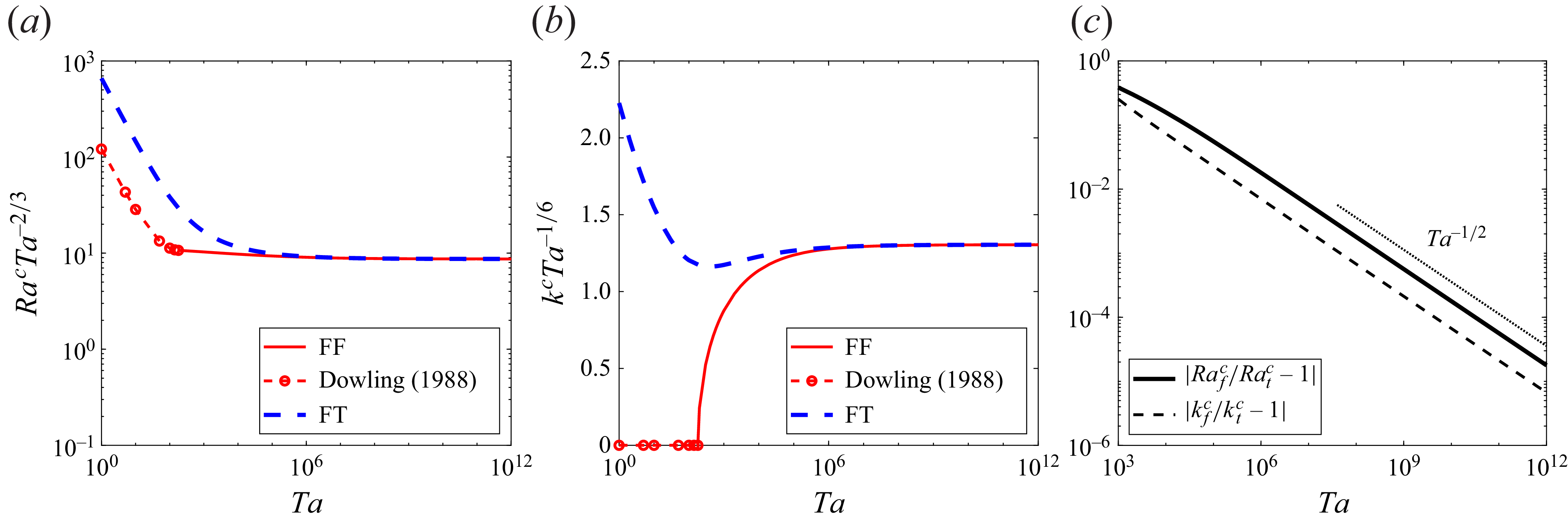


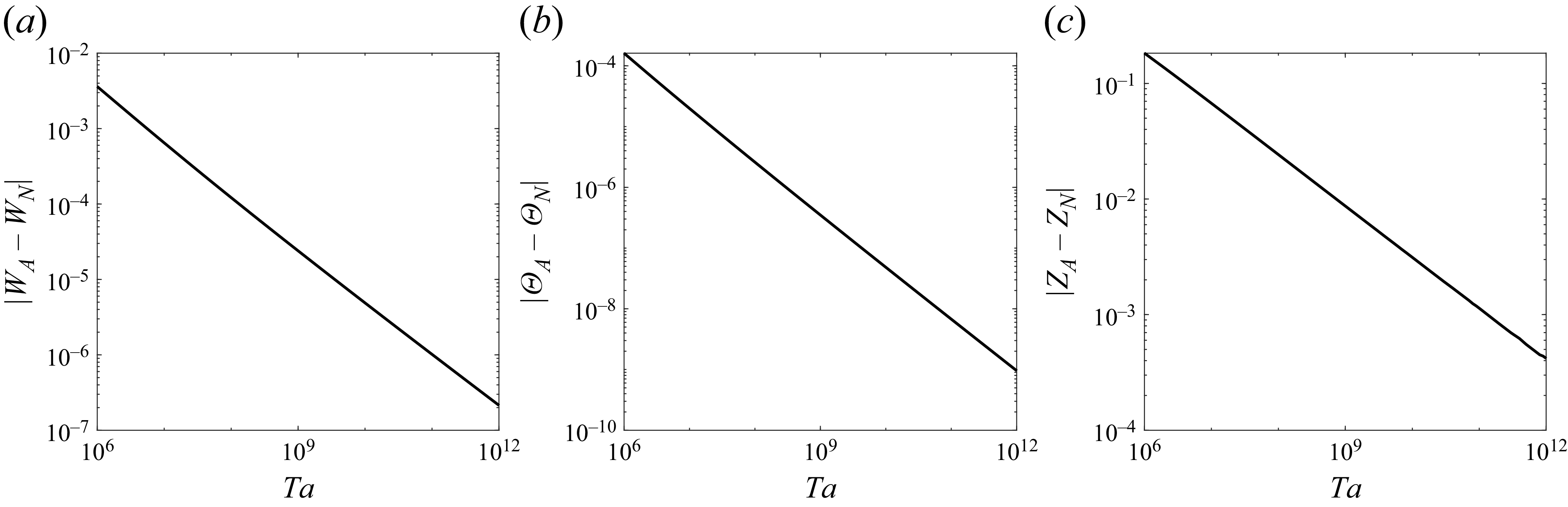


 Open access