Introduction

The Greenland ice sheet plays a crucial role in regulating global climate through its influence on the planetary albedo (Reference PatersonPaterson, 1994), and changes of the Greenland ice-sheet surface can have a distinct influence on the climatic conditions in Europe and worldwide (Reference Clark, Marshall, Clarke, Hostetler, Licciardi and TellerClark and others, 2001, Reference Clark, Pisias, Stocker and Weaver2002). Observing the Greenland ice sheet is therefore critical, but due to its vastness and remote location it is difficult to get a precise measure of changes in the ice sheet. To address this problem among others, the EuroClim project was initiated under the European Union’s Information Society Technology (IST) programme with the aim to produce a system to monitor climate change in Europe, including Greenland. The main goal of the project is to develop an advanced climate monitoring and prediction system for Europe, which will contribute to Europe’s ability to take the necessary measures to limit the consequences of climate change for human lives and society in general. The project has developed a distributed system where climate observations are collected by climate research institutes across Europe and integrated into a single database with a unified user interface. The project has also established a common methodology to acquire, process and store cryospheric data, and analyze long-term time series of data to estimate climatic trends. The system focuses on the European cryosphere, including the Arctic region, high mountain areas with seasonal snow and Greenland. The subsystem presented here utilizes the moderate-resolution imaging spectroradiometer (MODIS) sensor on the Terra satellite to monitor the Greenland ice sheet in a systematic way. The MODIS sensor produces a global dataset on a daily basis, with a resolution varying between 250m and 1 km, in 36 bands covering visible to thermal wavelengths. As part of the EuroClim project, we have monitored the extent of three different surface types, or facies, on the Greenland ice sheet on a monthly basis over the last 6 years, namely glacier ice, wet snow and dry snow. The percolation zone is here included in the wet snow category when the melting season begins following the standard characteristics for the accumulation zone (Reference BensonBenson, 1961; Reference PatersonPaterson, 1994). For each month the average, minimum and maximum extent of each facies have been derived. The results have been stored as monthly products available through the internet on the open EuroClim data distribution system (http://www.euroclim.net). Our emphasis has been to produce a widely available consistent dataset that can and will be produced routinely on a long-term basis for the purpose of monitoring climate change on the Greenland ice sheet. Here we report on the methodology and validation of the surface type derivation as well as the first 6 years of data from the Greenland ice sheet.

Methods

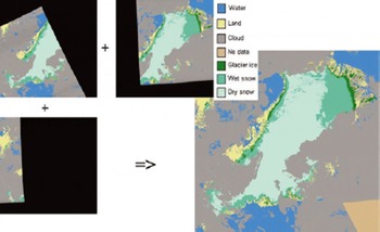
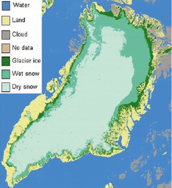
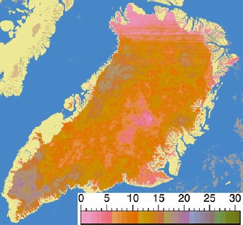
The algorithm products are created, following standards from the EuroClim project, as a sequence of products beginning with the classification and assembly of selected satellite images to produce a daily mosaic of the whole of Greenland (Fig. 1). Normalized indices of spectral bands are used and different threshold values are set up for each of the surface classes. Normalized indices are preferred because they help to compensate for changing physical parameters (e.g. illumination condition, surface slope). This is a general method and it is applied to all visible pixels on the satellite image (Reference Lillesand and KieferLillesand and Kiefer, 2000). All daily classification results within 1 month are reprojected to the EuroClim grid, where cloud-free ice-sheet pixels form the basis for the generation of monthly products. After 1 month, the most frequently occurring cloud-free class in a single pixel is chosen as the monthly class for that pixel. This allows the exclusion of pixels with cloud cover and provides the best estimate for each pixel during that month. This estimate varies in quality, and for every daily mosaic in which a pixel is classified as a cloud pixel the monthly classification result becomes less reliable. Figure 2 shows an example of a monthly glacier surface type (GST) product. The number of class occurrences is provided for each pixel. The proportion of days when a pixel is cloud-free serves as a measure of the reliability of the classification for each month (Fig. 3). The glacier melt area (GMA) product is derived directly from the GST classification results and it is the combined area of wet snow and glacier ice.

Fig. 1.

Example of a daily mosaic product. See text for more information.

Fig. 2.

Example of a monthly product generation. The glacier melt area (GMA) is the combined area of wet snow and glacier ice. See text for more information.

Fig. 3.

Number of observations plotted for each visible pixel within the ice-sheet mask. The number of observations is calculated for every monthly product in order to quantify the level of uncertainty for each product.

Algorithm and Product Description

The algorithm uses the MOD021KM data product to identify the different surface classes on the ice sheet. The data product contains calibrated and geolocated radiances for all 36 MODIS bands on a 1 km grid. The algorithm uses the visible and near-infrared reflectance and uses normalized thresholds to classify each pixel in the satellite image. The geolocation product MOD03 is used for masking land/water on a 1km resolution grid. The accuracy of the MODIS product MOD03 has been tested and found to be reliable within one to two pixels. This is satisfactory for the EuroClim purpose. The test has been carried out by direct comparison between measured global positioning system (GPS) positions of prominent features in South, West and East Greenland and the geocoded MODIS images. Cloudy pixels are identified with the MODIS cloud product MOD35_L2.

Because several reflectance bands in the MODIS range are used for the surface classification algorithm, the resolution of the product has been set to the common resolution of 1 km per pixel. Additional criteria are introduced in order to exploit the differences in spectral reflectance. Only cloud-free pixels, identified as land pixels, are used in the classification scheme. For the basic distinction between the ice/snow surface and bare land, the pixel is tested with the MODIS normalized snow difference index (NSDI) and a threshold for the band ratio between band 1 (620–670 nm) and band 7 (2105–2155 nm). The combination of these tests allows a more secure discrimination of ice/snow pixels, especially from non-glaciated surfaces where ice still shows higher reflectance values in band 1. The reflectance of snow and ice is sensitive to crystal size, and the sensitivity is largest at 1.0–1.3 μm (near-infrared) and smallest in the visible spectrum (Reference Nolin and DozierNolin and Dozier, 1993). The presence of liquid water in snow does not greatly affect the reflectance. During the melting season, meltwater will, however, change the crystal size and, by that, the reflectance (Reference Painter, Roberts, Green and DozierPainter and others, 1998).

Tests with false-color composites of the MODIS data were made in order to differentiate spectral variability in snow/ice facies in the visual and near-infrared parts of the spectrum. A clear difference is seen between snow and ice in these images, and the presence of melting can be detected due to its influence on the structure/size of snow and ice crystals. The algorithm was also tested on a number of MODIS scenes in areas where observations were available (Reference Podlech, Mayer and BøggildPodlech and others, 2004). The combination of the previously mentioned tests has shown that a threshold for normalized indices between the near-infrared band 5 (1230–1250 nm) and the visible band 10 (483–493 nm) gives good results for the distinction between different snow/ice facies.

In short, the following steps are followed for the classification of ice and snow surfaces: Information on clouds, water and ‘no data’ comes from the cloud mask (MOD35_L2). The ratio of band 1/band 7 < 0.0046, together with band 1 > 100, is used for an additional distinction between snow/ice and land. Bands 5 and 10 are used to derive normalized thresholds between dry snow, wet snow and ice,

(1)

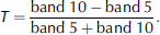
The thresholds were determined using the above-mentioned tests and methods. They are given as T(1) < 0.8 = dry snow, 0.8 < T(2) < 0.88 = wet snow, T(3) > 0.88 = glacier ice.

Validation

The validation of the threshold values for the different surface types was carried out using two complementary methods: visual comparison with satellite images from sensors (Advanced Thermal Emission and Reflection Radiometer (ASTER), QuikSCAT) and direct comparison with field observations. For the visual comparison, three validation periods were chosen: May–September 2002, May– September 2003 and May–September 2004. The visual comparison was carried out between high-resolution satellite images (ASTER), the raw MODIS MOD021KM data and the classification result. This visual comparison was carried out for a number of dates and areas along the perimeter of the Greenland ice sheet. This visual check worked very well for the ice–snow boundary, because it was easy to detect this boundary in the visible and shortwave infrared bands. The results from the visual comparison are illustrated in Table 1. The visual comparison is termed a ‘good comparison’ if most of the features on the ASTER image, raw MODIS image and classification results are similar so that glacier ice is, for example, observed in roughly the same places. An ‘acceptable’ comparison is derived when the same surface classes are seen but not necessarily in exactly the same places. A ‘not good’ comparison is derived when few or none of the surface classes match with the other satellite products.

Table 1.

Visual comparison between daily classification result, ASTER and QuikSCAT products. The total number is all the attempted visual comparisons for any given year. G: good comparison; AC: acceptable comparison; NG: bad comparison; NA: not available. The relative frequency is calculated between G/AC and NG data and reflects the success rate of the validation method

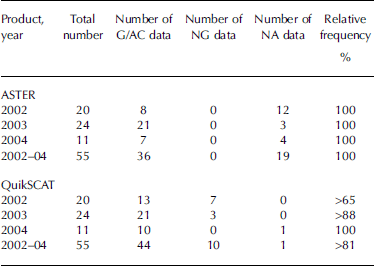
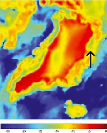
Table 1 also shows the results of visual comparison between QuikSCAT images and the classification results using the same notation as before. The SeaWinds scatterometer on QuikSCAT is an active microwave radar (Ku-band sensor) designed to measure electromagnetic backscatter from wind-roughened ocean surfaces. Backscattering of microwave signals from snow-/ice-covered surfaces depends on the roughness and electrical properties which, in turn, depend on the physical characteristics of the snow and ice cover. For example, liquid water dramatically changes the permittivity, and thus the microwave scattering signatures of snow (Reference Long and DrinkwaterLong and Drinkwater, 1999). The ground resolution of the QuikSCAT data is much less than the 1 km grid size used for the EuroClim products. The boundary between wet and dry snow can, however, be validated within five to seven EuroClim pixels by comparison of the classification results with the QuikSCAT products. A visual comparison has been carried out for several daily mosaic products during the validation periods as shown in Table 1 and Figures 4 and 5 for example. The dry snow is characterized by a low backscatter value, which can be seen in the center of the ice sheet. This is mainly due to the relatively small crystal size of dry snow allowing the microwaves to penetrate relatively deep into the snowpack where they are absorbed, hence the low backscatter. Backscatter increases when meltwater refreezes within the snowpack, causing crystal growth and the formation of ice lenses. Low backscattering values are also seen along the edges of the ice sheet (Fig. 4) where most of the melting occurs during the summer. Changes in the surface reflection due to melting may also result in a low backscatter value (Reference Long and DrinkwaterLong and Drinkwater, 1999). To illustrate the validation method, Figures 4 and 5 are used to detect similar features in the two products. See, for example, the large area around 79-fjorden in northeast Greenland, where both products yield roughly the same classification. The visual comparison with the QuikSCAT product must, however, be regarded with some reservation due to the difference between what the instruments measure. The active microwave radar penetrates into the surface of snow and will consequently contain information about subsurface layers as well (Reference Long and DrinkwaterLong and Drinkwater, 1999; Reference Nghiem, Steffen, Neumann and HuffNghiem and others, 2005). The GST, concerning the wet-snow/dry-snow boundary, can then only be compared to a certain degree with QuikSCAT products. For example, new snow in the wet snow zone can cover the surface for days. The daily product algorithm may then classify this new snow into the dry snow surface class, whereas the QuikSCAT instrument may still classify this into a wet snow surface class. This may also be a problem with respect to wet-snow/glacier-ice classification. The visual comparisons with both ASTER and QuikSCAT are summarized in Table 1. In total for all periods, ASTER yielded 36 successful classification results out of 36 (100%), and QuikSCAT yielded 44 successful classification results out of 54 (>81%).

Fig. 4.

Example of a QuikSCAT product for day of year 200 in 2003, which is used in the validation of the classification algorithm. The color bar is in dB. The low backscatter in the center of the ice sheet represents the dry snow, and the arrow points at the area around 79-fjorden where melting is present.

Fig. 5.

Example of a daily classification product for day of year 200 in 2003. This product is compared visually with the QuikSCAT product and ASTER image in order to validate the classification algorithm. The arrow points at the area around 79-fjorden where melting is present.

Direct comparison with field observations was carried out in areas where ground-truth data were available. Surface observations have been carried out in the areas of the Qagssimiut lobe, Nuuk and Tasiilaq. Typically, the measurements were carried out at the beginning (early May) or the end (mid-September) of the ablation season at different altitudes on the ice sheet. The observations plotted are near-surface temperature, albedo, incoming solar radiation, daily classification result and tilt of station (Fig. 6). The temperature provides a basis for determining whether the surface is melting or freezing at the observation site. Following the positive air temperatures during the summer, the dry-snow category changes into the wet-snow category as a result of snowmelt. When all the snow is melted, the category will change into glacier ice. Changes in the albedo also reflect changes on the surface, where high values correspond to snow and low values correspond to glacier ice and other surfaces with relatively high absorption. The tilt of the stations is also plotted, in order to provide confidence in the albedo measurements, since these become unreliable at a tilt of more than ±5˚. The incoming solar radiation reveals whether the sky is cloudy or clear.

Fig. 6.

Daily classification results compared with observations from an automatic weather station placed on the ice sheet near the town of Tasiilaq (65˚42.163′ N, 38˚51.926′W; 600ma.s.l.). See text for more information.

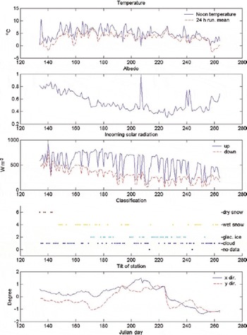
See Table 2 for a summary and Figure 6 for an example of the observation data. Inspection of the observations at the Nuuk station shows that the near-surface air temperature was almost invariably positive, supporting the classification results, which show no dry snow. As the albedo measurements are only reliable until day 200 due to the increasing tilt of the station, only the 38 daily classification results up to that point can be validated. Out of these, 6 points are ‘no data’ and must be excluded, leaving a total of 32 remaining classification results. Comparing the 21 clear-sky results with the albedo to determine whether the surface is ‘wet snow’ or ‘glacier ice’ yielded 16 instances correctly classified as ‘wet snow’ and 5 correctly classified as ‘glacier ice’, whereas one classification as ‘glacier ice’ should have been ‘wet snow’. There were no ‘dry snow’ classification results. This gives 20 out of 21 correct distinctions between surface classes (>95%). Out of the 11 results classified as ‘cloudy’, only two did not appear to be cloudy from comparisons with the reduction of incoming shortwave radiation due to clouds in the station data. Thus we arrive at a total of 29 successful classification results out of 32 (>90%). Note that the two erroneous classifications as ‘cloudy’ may actually be correct as the cloud conditions can change rapidly. A similar comparison of the daily classification results with the station data from the ice sheet near Tasiilaq yielded a correct distinction of surface type classes in 56 out of 67 cases (>83%). All 61 ‘cloudy’ classification results seemed correct, giving a total of 117 out of 128 correct classifications (>91%). For the comparison with the station data near Narssaq, there were 57 correct surface type distinctions out of 60 (95%), and a total of 117 out of 124 classification results when including the ‘cloudy’ results (>94%). The total for all sites is then 133 successful surface type classification results out of 148 (>89%). Including the cloud classification yields a total of 263 correct daily classifications out of 284 (>92%).

Table 2.

Daily classification results compared with observations from AWSs placed on the ice sheet, near the towns of Nuuk (64˚44.174⁰ N, 49˚29.555⁰W; 900ma.s.l.), Tasiilaq (65˚42.163⁰ N, 38˚51.926⁰W; 600ma.s.l.) and Narssaq (Sermilik) (61˚01.525⁰ N, 46˚52.270⁰W; 350ma.s.l.). The total relative frequency is a measure of the success of the validation method

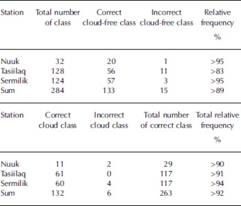
These field observations were used, together with satellite data, in the validation of the thresholds for the algorithm. For areas further to the north, only comparison with satellite data was used to test the classification algorithm. The visual comparison with satellite data and field observations worked well based on the majority (ASTER = 100% and Quik-SCAT = 81%) of ‘Good’ and ‘Acceptable’ visual comparisons and with the high numbers of successful classifications when compared to the observations (>92%).

Results

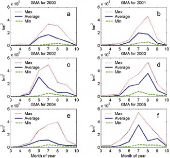
Daily classification results, such as those shown in Figure 1, are used to calculate a monthly glacier surface type classification result (GST product) (see Fig. 2). Non-ice-sheet areas are eliminated with an ice-sheet mask, to provide a standard basis for further processing and derived product calculations such as the glacier melt area (GMA product). The GMA product was calculated from every GST product and is shown in Figures 7 and 8. The three different graphs on each plot represent the maximum, average and minimum extent of the GMA, respectively. The maximum GMA is calculated using every cloud-free pixel from a satellite image, and if one pixel during that month has experienced one day of melting, i.e. the classification was wet snow or ice, the pixel gets that classification. The maximum GMA product thus contains information about brief melt events during the melting season. In the case of the minimum GMA, a pixel is classified as dry snow if it receives that classification at least once during a month. This will therefore reveal areas experiencing consistent melting during the summer period. For the average GMA, pixels are classified on the basis of the most frequently occurring cloud-free class during a month.

Fig. 7.

GMA products, March–October: (a) 2000; (b) 2001; (c) 2002; (d) 2003; (e) 2004; and (f) 2005.

Fig. 8.

GMA products for melt area against year, with separate curves for each month: (a) March; (b) April; (c) May; (d) June; (e) July; (f) August; (g) September; and (h) October. 0 is year 2000 and so on.

The results shown in Figures 7 and 8 show that a lot of variation is present during the 6 year period and that 2002, 2003 and 2005 experienced strong melting compared to the other years. The timing of melt onset and length of the melt season differ substantially between years. In some years the melting season evolves slowly, while in other years the melt area grows rapidly and decreases slowly. 2002 is an example of an intense onset of melting followed by a slow decrease. 2003 was a long melt season, which started relatively intensely, gradually increased until August and ended in October. It should also be noted that 2005 was unusual in many ways. Melting was already detected in March, gradually increased until July and declined thereafter. September 2005 yielded a larger melt area than August 2005, something that did not occur in other years. This may be due to a single large melt event or in general because there is a low-quality performance of the algorithm for the MODIS data in both August and September 2005. The low-quality performance of the classification results in many pixels with ‘no data’. Data from automatic weather stations in the southern part of Greenland show a similar trend between positive air-temperature data, albedo data and the classification product for 2003 and 2004. Reference Podlech, Mayer and BøggildPodlech and others (2004) used a positive degree-day model in order to estimate the ablation in the same area as the data shown in Figure 6. These data show a gradual increase in ablation from 2000 to 2002. In relation to this, the results in Figures 7 and ˚ also show an increase in melt area, which may be related to the surface mass balance of the ice sheet.

Reference Steffen, Nghiem, Huff and NeumannSteffen and others (2004) described the melt anomaly on the Greenland ice sheet in 2002 using active and passive microwave data (scanning multichannel microwave radiometer (SMMR), Special Sensor/Microwave/Imager (SSM/I), QuikScat). This strong melt anomaly in 2002 is also seen in Figure 7. Reference Steffen, Nghiem, Huff and NeumannSteffen and others (2004) describe 2003 as a long melt season, which is also seen in Figure 7. There is a good similarity between the EuroClim products and the products derived by Reference Steffen, Nghiem, Huff and NeumannSteffen and others (2004).

Discussion and Conclusions

A new cryospheric monitoring system for the Greenland ice sheet was created using daily images from the MODIS sensor. The quality of the products depends on the time of day, as the elevation of the sun above the horizon needs to be high in order to reduce any shadow effects from clouds and mountains. This gives a more reliable image when the classification starts. All data used are therefore from the middle of the day (1300–1700 h). This also gives a better representation of the melt areas because the effect of the sun is largest in the middle of the day. Changes of the ice-sheet margin are not taken into account, because the potential changes over one decade are not expected to exceed the dimension of one pixel. The energy balance of ice-sheet surfaces strongly depends on surface characteristics, where the albedo can change from about 0.8 for fresh snow to 0.4–0.6 for bare ice and even less for meltwater ponds (Reference PatersonPaterson, 1994). During the summer season, the surface of the Greenland ice sheet changes from a uniform dry snow surface to a highly variable surface, ranging from pure old ice at the margin to dry, highly reflective snow in the center of the ice sheet. As melting proceeds, more ice is exposed in the lower areas and superimposed ice is created in the lower part of the wet snow zone (Reference BensonBenson, 1961; Reference PatersonPaterson, 1994). The snowline divides the ice surface areas from the snow-covered areas, whereas the dry-snow line marks the upper limit of surface melting. The difference in spectral reflectance between superimposed ice and glacier ice is very small and difficult to detect. This makes it difficult to determine the equilibrium line, at least with optical sensors (Reference König, Winther and IsakssonKönig and others, 2001). The fieldwork activities show the progress of surface changes during the summer, and the classification results show consistent changes with respect to the derived surface classes. Reference Hall, Williams and CaseyHall and others (2006) have studied the surface temperature variability of the Greenland ice sheet using MODIS data over roughly the same period and they conclude that migration of ice-sheet facies to higher altitude reflects changes in the mass balance.

The 1 km resolution data used here work well for determining the different surface classes on the ice sheet.

Smaller features will, of course, not be represented correctly. The spectral fingerprint of all landscape parameters changes with the ground resolution, and some features may fall into the wrong category. It is therefore necessary to bear in mind that the relationship between the spatial resolution of the sensor, the spatial structure of the environment under investigation, and the nature of the information sought in any given image-processing operation always plays a role in digital image processing (Reference Lillesand and KieferLillesand and Kiefer, 2000). The uncertainties associated with the derived melt areas and distribution of the different surface types are assessed with the number of observations for each cloud-free pixel (Fig. 4). This makes it possible to judge how often a pixel was observed during a given month. This is also a measure of the reliability, both temporal and spatial, in relation to the variability of the product’s quality. The loss of data due to clouds is the primary source of uncertainties. However, the MODIS data also have advantages, such as high spatial resolution (1 km) and high spatial and temporal coverage. The rationale for a monthly product is the creation of a cloud-free image that describes the area where melting occurred on the ice sheet during 1 month.

The algorithm was validated with the use of scatterometer data from the QuikSCAT satellite. One could then argue that the above-mentioned results should be similar, but Quik-SCAT was only one tool used in the validation, and, as argued before, the results may differ due to the difference between the sensors. One of the strengths of the QuikSCAT data is the very consistent daily product with zero cloud-cover limitation, but the poor resolution is a major weakness of the products. The low resolution of QuikSCAT data compared with MODIS data sets a natural limit on the visual validation of the algorithm. The wet-/dry-snow and wet-snow/glacier-ice zones can only be interpreted within five to seven EuroClim pixels when compared. This may account for some of the discrepancies between EuroClim products and interpretations of the QuikSCAT data (Reference Steffen, Nghiem, Huff and NeumannSteffen and others, 2004; Reference Nghiem, Steffen, Neumann and HuffNghiem and others, 2005). Impurities in snow, such as continental dust and anthropogenic aerosols, may affect the reflectance. The impurities in the snow will reduce the reflectance in the visible part of the spectrum, where snow and ice are normally highly reflective (Reference Dozier and PainterDozier and Painter, 2004). This reduction in reflectivity could classify wet snow as glacier ice or even dry snow as wet snow if the reduction is large enough. However, this may not be very significant in the dry snow zone, but could have a larger effect close to the margin.

The classification algorithm and methodology used have the advantages of easy implementation, automatic processing and straightforward data classification, and the product validation showed that the products from the algorithm have potential as indicators of the impact of climate change and variability on the Greenland ice sheet. The MODIS products should be viewed as complementary to existing products, such as the Greenland temperature product by Reference Hall, Williams and CaseyHall and others (2006) and the Greenland melt area product by Reference Steffen, Nghiem, Huff and NeumannSteffen and others (2004). The potential users of the products may be researchers with a background in cryospheric research or European governments in relation to their environmental policy. The products are easy to use and have the potential to be used as input parameters and validation targets in climate models that include cryospheric processes in Greenland.

Over the last 5 years the EuroClim project has created a strong tool for cryospheric monitoring, and its products can be used by everyone interested in the cryosphere. The algorithm presented here covers the largest area in the EuroClim system and provides potential users with a consistent product in the further investigation of the Greenland ice sheet and the Arctic region. Future fieldwork activities planned in relation to a monitoring effort on the Greenland ice sheet will allow a further improvement in the field validation of the EuroClim product.