


INTRODUCTION
Tides and ocean swell produce ice-shelf flexure, and thus, can initiate break-up of ice in those ice shelves and encourage ice-shelf rift propagation (Holdsworth and Glynn, Reference Holdsworth and Glynn1978; Goodman and others, Reference Goodman, Wadhams and Squire1980; Wadhams, Reference Wadhams and Untersteiner1986; Squire and others, Reference Squire, Dugan, Wadhams, Rottier and Liu1995; Meylan and others, Reference Meylan, Squire and Fox1997; Bromirski and others, Reference Bromirski, Sergienko and MacAyeal2009). No strong correlation between rift propagation rate and ocean swell has been revealed so far (Bassis and others, Reference Bassis, Fricker, Coleman and Minster2008), and it is not clear to what degree the rift propagation can be triggered by tides and ocean swell. Nevertheless, the impact of tides and ocean swell is a significant fraction of the total force (Bassis and others, Reference Bassis, Fricker, Coleman and Minster2008) that produces ice calving in ice shelves (MacAyeal and others, Reference MacAyeal2006). Moreover, the resonant-like motion that can occur under suitable conditions of long-term swell forcing (sustained impact over many swell periods) can cause fracture in the ice-shelf (Holdsworth and Glynn, Reference Holdsworth and Glynn1978). Thus, insight into the process of vibration in ice shelves is important for understanding ice-sheet–ocean interactions and ice-shelf stability.
Models of ice-shelf flexure and vibrations have been proposed (e.g. Robin, Reference Robin1958; Holdsworth, Reference Holdsworth1977; Hughes, Reference Hughes1977; Holdsworth and Glynn, Reference Holdsworth and Glynn1978; Goodman and others, Reference Goodman, Wadhams and Squire1980; Lingle and others, Reference Lingle, Hughes and Kollmeyer1981; Stephenson, Reference Stephenson1984; Wadhams, Reference Wadhams and Untersteiner1986; Smith, Reference Smith1991; Vaughan, Reference Vaughan1995; Schmeltz and others, Reference Schmeltz, Rignot and MacAyeal2001; Turcotte and Schubert, Reference Turcotte and Schubert2002), based on elastic thin-plate/elastic-beam approximations. These models provide simulations of ice-shelf deformations, calculate the bending stresses due to the vibrations and assess possible effects of tides and ocean swell impacts on the calving process.
Further development of elastic-beam models for the description of ice-shelf flexure used visco-elastic rheological models. In particular, tidal flexures of an ice-shelf were obtained using the linear visco-elastic Burgers model (Reeh and others, Reference Reeh, Christensen, Mayer and Olesen2003; Walker and others, Reference Walker2013), and the non-linear 3-D visco-elastic full-Stokes model (Rosier and others, Reference Rosier, Gudmundsson and Green2014). An analytical approach, in which flexural motions of ice cover were described by the Timoshenko–Mindlin equation, was undertaken by Balmforth and Craster (Reference Balmforth and Craster1999), whereas Sergienko (Reference Sergienko2010) derived exact analytical solutions that describe ice-shelf deformation and stress induced by long ocean waves in an idealized ice/ocean geometry (in a non-resonant case).
Here, the modeling of forced vibrations of a buoyant, uniform, elastic ice tongue, floating in shallow water of variable depth, is developed. Simulations of ice-shelf flexure are performed by a full 3-D finite-difference elastic model. The model features a combination of boundary conditions applied to the ice plate, which are linear combinations of the typical form of boundary conditions with those developed in Konovalov (Reference Konovalov2015, Reference Konovalov2016). The main objective of this study is to obtain the amplitude spectra for the floating ice-shelf using the full finite-difference elastic model, focusing on the eigenvalue problem for ice-shelf vibrations in 3-D elastic models. In this study, the term ‘eigenvalue’ is employed in the same meaning as in a Sturm–Liouville Eigenvalue Problem (e.g. Tikhonov and Samarskii, Reference Tikhonov and Samarskii1963).
In nature, the probability of random wave events arriving at an ice-shelf with a specific (fixed) frequency is equal to zero (wave arrivals always display a range of frequencies which vary continuously with arrival time). There is, however, a non-zero probability that the random wave event will cover a range of frequency that contains specific frequencies to which the ice-shelf/ocean system is sensitive. The specific resonant frequencies for ice-shelf/ocean systems determined alone, without information about how the response of the ice-shelf/ocean system varies within a small range of frequency surrounding the resonance is thus not fully sufficient. By determining the width of ice-shelf/ocean resonance spectra surrounding the exact resonance frequency, the ‘compatibility’ of the system to be excited by random wave events is thus better determined.
FIELD EQUATIONS
Basic equations
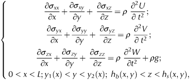
The 3-D elastic model is based on the well-known momentum equations (e.g. Landau and Lifshitz, Reference Landau and Lifshitz1986; Lamb, Reference Lamb1994):
 $$\left\{ {\matrix{ {\displaystyle{{\partial \sigma_{xx}} \over {\partial x}} + \displaystyle{{\partial \sigma_{xy}} \over {\partial y}} + \; \displaystyle{{\partial \sigma_{xz}} \over {\partial z}} = \rho \; \displaystyle{{\partial^2U} \over {\partial \; t^2}};\; \;} \cr {\displaystyle{{\partial \sigma_{yx}} \over {\partial x}} + \displaystyle{{\partial \sigma_{yy}} \over {\partial y}} + \; \displaystyle{{\partial \sigma_{yz}} \over {\partial z}} = \rho \; \displaystyle{{\partial^2V} \over {\partial \; t^2}};} \cr {\displaystyle{{\partial \sigma_{zx}} \over {\partial x}} + \displaystyle{{\partial \sigma_{zy}} \over {\partial y}} + \; \displaystyle{{\partial \sigma_{zz}} \over {\partial z}} = \rho \; \displaystyle{{\partial^2W} \over {\partial t^2}} + \rho g;} \cr {0 \lt x \lt L;y_1(x) \lt y \lt y_2(x);\; h_b(x,y) \lt z \lt h_s(x,y),} \cr}} \right.$$
where (XYZ) is a rectangular coordinate system with X axis along the central line, and Z axis is pointing vertically upward; U,V and W are two horizontal and one vertical ice displacements, respectively; σ is the stress tensor; and ρ is the ice density. The ice-shelf is of length L along the central line. The geometry of the ice-shelf is assumed to be given by lateral boundary functions y 1,2(x) at sides labeled 1 and 2 and functions for the surface and base elevation, h s,b(x, y), denoted by subscripts s and b, respectively. Thus, the domain on which Eqn (1) is solved is Ω = {0 < x < L, y 1(x) < y < y 2(x), h b(x, y) < z < h s(x, y)}.
Sub-ice water is assumed to be an incompressible inviscid fluid of uniform density. Another assumption is that the water depth in the cavity below the ice-shelf changes gradually in the horizontal directions. Thus, the ice front and other such features are not considered here. Moreover, the ice is considered to be a continuous solid elastic plate. Under these three assumptions, sub-ice water flow is independent of z in a vertical column. Manipulating the governing equations of the shallow sub-ice water layer yields the wave equation (Holdsworth and Glynn, Reference Holdsworth and Glynn1978):
 $$\displaystyle{{\partial ^2W_{\rm b}} \over {\partial \; t^2}} = \; \displaystyle{1 \over {\rho _{\rm w}}}\; \displaystyle{\partial \over {\partial \; x}}\; \left( {d_0\displaystyle{{\partial \; P{\rm^{\prime}}} \over {\partial \; x}}} \right)\; + \; \displaystyle{1 \over {\rho _{\rm w}}}\displaystyle{\partial \over {\partial \; y}}\left( {d_0\displaystyle{{\partial \; P{\rm^{\prime}}} \over {\partial \; y}}} \right),$$
where ρ w is the sea water density; d 0(x, y) is the depth of the sub-ice water layer; W b(x, y, t) is the vertical deflection of the ice-shelf base and W b(x, y, t) = W(x, y, h b(x, y), t); and P ′(x, y, t) is the deviation of the sub-ice water pressure from the hydrostatic value.
Boundary conditions
The boundary conditions are: (i) a stress-free ice surface; (ii) the normal stress exerted by seawater at the ice-shelf-free edges and at the ice-shelf base; and (iii) rigidly fixed edges at the grounding line of the ice-shelf.
In this model, the boundary conditions are considered in the form of the linear combination
 $$\alpha _1\; F_i(U,V,W) + \; \alpha _2\; {\rm \Phi} _i(U,V,W) = 0,\; \; i = 1,2,3,$$
where:
(i) F i(U, V, W) = 0 is the typical and a well-known form of the boundary conditions where, e.g. the condition on the ice-shelf surface is expressed as σ ik n k = 0 ( $\vec{n}$ is the unit vector normal to the surface);
(ii) Φi(U, V, W) = 0 is the approximation developed in Konovalov (Reference Konovalov2015, Reference Konovalov2016); and
(iii) the coefficients α 1 and α 2 satisfy the condition α 1 + α 2 = 1.

Thus, these boundary conditions (3) are the superposition of the typical boundary conditions and those developed in Konovalov (Reference Konovalov2015, Reference Konovalov2016). The boundary conditions formulated here are notable because they are ‘mixed’, i.e. they represent what is typically seen in the previous studies adjusted for the physical considerations presented in Konovalov (Reference Konovalov2015, Reference Konovalov2016).
Discretization of the model
The numerical solutions were obtained by a finite-difference method, which is based on the standard coordinate transformation
 $$x,y,z\; \to x,\; \;\eta = \displaystyle{{y-y_1} \over {y_2-y_1}},\; \;\xi = (h_{\rm s}-z)/H,$$
where H is the ice thickness (H = h s − h b). The coordinate transformation maps the ice domain Ω into the rectangular parallelepiped Π = {0 ≤ x ≤ L;0 ≤ η ≤ 1;0 ≤ ξ ≤ 1}, which presents simplification to the numerical discretization.
Equations for ice-shelf displacements
Constitutive relationships between stress tensor components and displacements correspond to Hook's law (e.g. Landau and Lifshitz, Reference Landau and Lifshitz1986; Lurie, Reference Lurie2005):
 $$\sigma _{ij} = \displaystyle{E \over {1 + \nu}} \left( {u_{ij} + \displaystyle{\nu \over {1-2\nu}} \; u_{ll}\delta_{ij}} \right),$$
where u ij are the strain components.
Substitution of these relationships into Eqn (1) gives final equations of the model:
 $$\left\{ \matrix{\displaystyle{{2(1-\nu )} \over {1-2\nu}} \displaystyle{{{\rm \partial}^2U} \over {{\rm \partial} x^2}} + \displaystyle{{{\rm \partial}^2U} \over {{\rm \partial} y^2}} + \displaystyle{{{\rm \partial}^2U} \over {{\rm \partial} z^2}} + \displaystyle{1 \over {1-2\nu}} \left( {\displaystyle{{{\rm \partial}^2V} \over {{\rm \partial} x{\rm \partial} y}} + \displaystyle{{{\rm \partial}^2W} \over {{\rm \partial} xdz}}} \right) = \displaystyle{{2(1 + \nu )} \over E}\rho \displaystyle{{{\rm \partial}^2U} \over {{\rm \partial} t^2}}; \hfill \cr \displaystyle{{{\rm \partial}^2V} \over {{\rm \partial} x^2}} + \displaystyle{{2(1-\nu )} \over {1-2\nu}} \displaystyle{{{\rm \partial}^2V} \over {{\rm \partial} y^2}} + \displaystyle{{{\rm \partial}^2V} \over {{\rm \partial} z^2}} + \displaystyle{1 \over {1-2\nu}} \left( {\displaystyle{{{\rm \partial}^2U} \over {{\rm \partial} y{\rm \partial} x}} + \displaystyle{{{\rm \partial}^2W} \over {{\rm \partial} ydz}}} \right) = \displaystyle{{2(1 + \nu )} \over E}\rho \displaystyle{{{\rm \partial}^2V} \over {{\rm \partial} t^2}}; \hfill \cr \displaystyle{{{\rm \partial}^2W} \over {{\rm \partial} x^2}} + \displaystyle{{{\rm \partial}^2W} \over {{\rm \partial} y^2}} + \displaystyle{{2(1-\nu )} \over {1-2\nu}} \displaystyle{{{\rm \partial}^2W} \over {{\rm \partial} z^2}} + \displaystyle{1 \over {1-2\nu}} \left( {\displaystyle{{{\rm \partial}^2U} \over {{\rm \partial} z{\rm \partial} x}} + \displaystyle{{{\rm \partial}^2V} \over {{\rm \partial} zdy}}} \right)-\displaystyle{{2(1 + \nu )} \over E}\rho g = \displaystyle{{2(1 + \nu )} \over E}\rho \displaystyle{{{\rm \partial}^2W} \over {{\rm \partial} t^2}}. \hfill} \right.$$
Ice-shelf harmonic vibrations: the eigenvalue problem
It is assumed that for harmonic vibrations, all variables are periodic in time, with the periodicity of the incident wave (of the forcing) given by the frequency ω, i.e.
 $$\tilde{\varsigma} (x,y,z,t) = \varsigma (x,y,z)\; e^{i\omega t},$$
where  $\tilde{\varsigma} = \{ U,V,W,\; \; \sigma _{ij}\} $, where we are interested in the real part of the variables expressed in a complex form.
This assumption also implies that the full solution of the linear partial differential Eqns (2) and (5) is a sum of the solution for the steady-state flexure of the ice-shelf and solution (6) for the time-dependent problem. In other words, solution (6) implies that the deformation due to the gravitational forcing can be separated from the vibration problem, i.e. the term ρg as well as the appropriate terms in the boundary conditions (3) are absent from the final equations formulated for the vibration problem, because a time-independent solution accounting for them applies and is not of interest in this study.
The separation of variables in Eqn (6) and its substitution into Eqns (2) and (5) yields the same equations, but with the operator ∂2/∂ t 2 replaced with the constant − ω 2, i.e. we obtain equation for  $\varsigma (x,y,z)$:
 $${\rm {\cal L}\;} \varsigma = -\omega ^2\varsigma, $$
where  ${\rm {\cal L}}$ is a linear partial differential operator.
The numerical solution of Eqn (7) at different values of ω yields the dependence of  $\varsigma $ on the frequency of the forcing ω. When the frequency of the forcing converges to the eigenfrequency of the system, we observe the typical rapid increase of deformation/stresses in the spectra in the form of the resonant peaks.
Note that here, the term ‘eigenvalue’ refers to the eigenfrequency (ω n) of the ice/water system or corresponding periodicity (T n = (2π/ω n)). As mentioned previously, the term ‘eigenvalue’ is employed in the same meaning like in a Sturm–Liouville Eigenvalue Problem (e.g. Tikhonov and Samarskii, Reference Tikhonov and Samarskii1963). Eigenvalues (where resonant peaks would be observed) are denoted by the letters ω n or T n with the subscript n (or other), which is an integer, because the array of the eigenvalues is a countable set.
Letters ω or T without the subscript denote the non-resonant values of frequency or periodicity of the ice/water system. They are defined by the frequency of the incident wave (of the forcing).
The eigenvalues can be derived from the equation D(ω) = 0, where D is the determinant of the matrix, which results from the discretization of Eqn (7) and of the corresponding boundary conditions. However, the probability of the appearance of the forcing at any specific frequency is practically zero. This can be seen when we consider only events within the frequency range (ω i − Δω, ω i + Δω). The probability of a forcing that is within the frequency range is non-zero:
 $$p\{ \omega \in (\omega _i-\Delta \omega, \; \; \omega _i + \Delta \omega )\} = \displaystyle{{2\Delta \omega} \over {\rm \Omega}}, $$
where Ω is the width of the range in omega space, which includes all possible frequencies of the forcing. Eqn (8) also assumes that the events have equal probabilities in different parts of Ω.
Thus, the probability of the resonant-like motion is higher when the value Δω, which is defined by the width of the resonant peak, is higher too. Therefore, the width of the resonant peaks is an important parameter, from a practical standpoint, because it defines the probability of the suitable resonant-like motion.
Computation of the spectra, such as provided below, thus provides important information about the width of resonant peaks within the likely range of forcing frequencies found in nature. By assessing the widths of such peaks, a better understanding of the probability that any one specific forcing event at a specific ω can be assessed.
NUMERICAL RESULTS
The numerical experiments with ice-shelf/tongue forced vibrations were carried out for a physically idealized ice-shelf with the geometry of a rectangular parallelepiped as described above. In the undeformed ice-shelf, the four edges had coordinates x = 0, x = L, y 1 = 0, y 2 = B, where L is the plate length along the X axis and B is the plate width along the Y axis (B = y 2 − y 1, see Eqn (1)). Furthermore, the ice-shelf thickness H = h s(x, y) − h b(x, y) was held constant in these experiments.
Experiment A
In Experiment A, the ice-shelf had two fixed edges (at x = 0, y 1 = 0) and two free edges (at x = L, y 2 = B) and the water layer was absent. This geometry represents the limiting case of an ice-shelf that is in vanishingly shallow water and which is only partially surrounded by land. In this experiment, the ice-shelf vibrations were generated by pressure that was uniformly distributed across the ice base and that periodically changed with time.
Under the given conditions, when two adjacent edges are fixed and two others are free, the analytical solution can be obtained by the thin-plate approximation (e.g. Landau and Lifshitz, Reference Landau and Lifshitz1986). In particular, the eigenfrequencies are expressed as
 $$\omega _{k,n} = \; \sqrt {\displaystyle{{E\; H^2} \over {12\rho \; (1-\nu ^2)}}} \; \; \pi ^2\; \left\{ {{\left( {\displaystyle{k \over L}} \right)}^2 + \; {\left( {\displaystyle{n \over B}} \right)}^2} \right\},\; \; k,n = 1,2 \ldots $$
Experiment A was undertaken for different values of the aspect ratio γ = H/L.
Figure 1 shows the amplitude spectra obtained in Experiment A. Here, ‘amplitude spectrum’ means the dependence of the deflection amplitude (taken to be the maximum value across the ice-shelf) on the frequency (of the incident wave/forcing). The deflection amplitude is normalized by the forcing amplitude. The amplitude spectra presented in Figure 1 were obtained for three values of the aspect ratio: (a) γ 1 = 5 · 10−2 (H = 100 m; Fig. 1a); (b) γ 2 = 2.5 · 10−2 (H = 50 m; Fig. 1b) and (c) γ 3 = 2.5 · 10−3 (H = 25 m; Fig. 1c); i.e. the changes in the aspect ratio were provided by the changing of ice thickness (H). Vertical lines in Figure 1 are aligned to the eigenfrequencies defined by Eqn (9). The amplitude spectra were obtained for different values of α 1 and α 2 from Eqn (3).
The amplitude spectra, maximal ice-shelf deflection vs periodicity of the forcing, obtained in Experiment A. Vertical lines correspond to the eigenfrequencies defined by Eqn (7). (a) Ice-plate dimensions are L = 2 km, B = 1 km, H = 100 m. Aspect ratio γ = 0.05. Сurves 1–4 are the amplitude spectra derived from the full model: 1 – α 1 = 1, α 2 = 0; 2 – α 1 = 0.8, α 2 = 0.2; 3 – α 1 = 0.6, α 2 = 0.4; 4 – α 1 = 0, α 2 = 1. (b) Ice-plate dimensions are L = 2 km, B = 1 km, H = 50 m. Aspect ratio γ = 0.025. The curve is the amplitude spectrum derived from the full model. (c) Ice-plate dimensions are L = 2 km, B = 1 km, H = 25 m. Aspect ratio γ = 0.0125. The curve is the amplitude spectrum derived from the full model. Young's modulus E = 9 GPa, Poisson's ratio ν = 0.33 (Schulson, Reference Schulson1999).
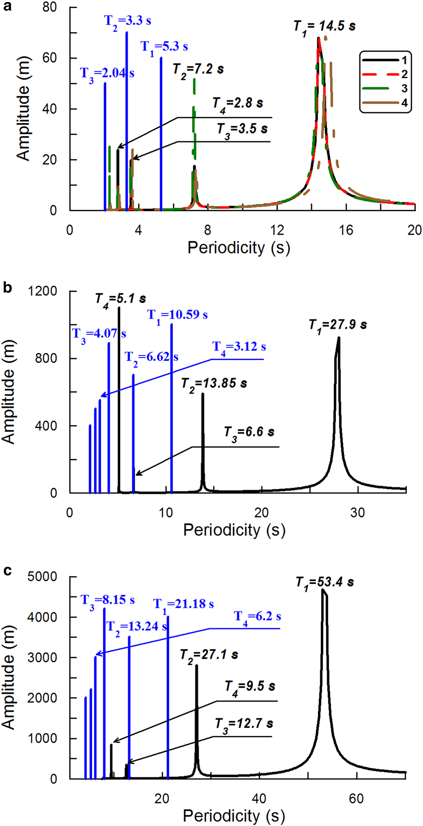
The eigenvalues derived by the full model and the ones obtained by Eqn (9) are different. However, as for both the exact solutions (9) and modeled spectra, the changes of the aspect ratio created similar changes in the spectra in agreement with the following ratio
 $$\displaystyle{{{(T_i)}_1} \over {{(T_i)}_2}} = \displaystyle{{\gamma _2} \over {\gamma _1}},$$
where (T i)k is the i-th eigenperiodicity that corresponds to the aspect ratio γ k. In particular, for the exact solutions the ratio (10) directly follows from Eqn (9), if the changes in the aspect ratio are provided by varying of ice thickness (H). This is because of the H 2 dependence of the parameters in the elastic flexure rigidity of the ice-shelf.
Experiment B
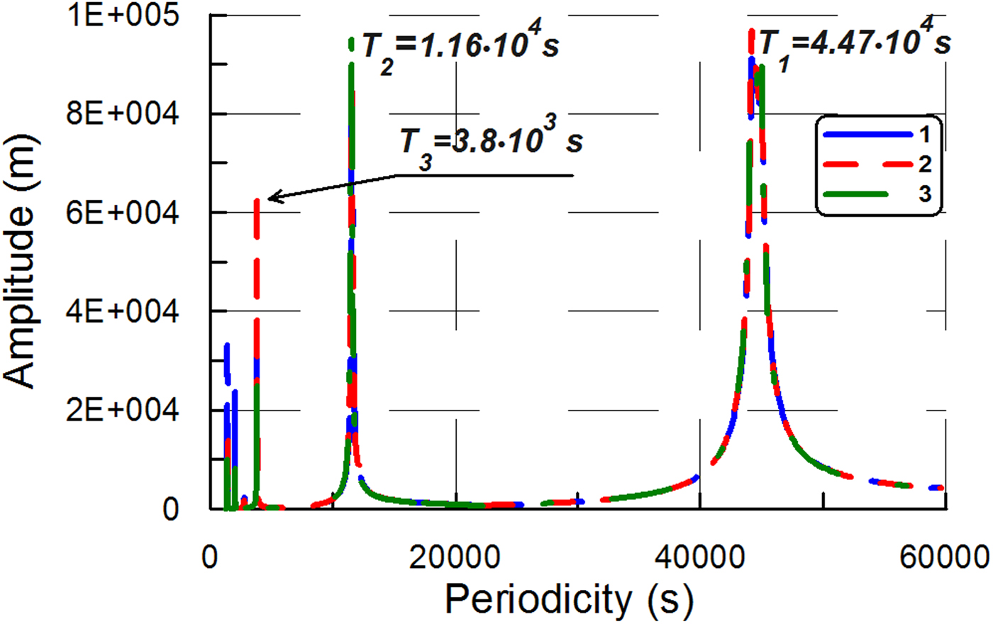
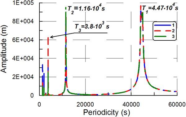
As in the previous experiment, in Experiment B the ice plate had two fixed edges (at x = 0, y 1 = 0) and two free edges (at x = L, y 2 = B), but the water layer was present and the layer depth was constant. The ice-plate dimensions were L = 20 km, B = 10 km, H = 100 m. The water-layer depth was d 0 = 100 m and the aspect ratio γ was equal to 5 · 10−3 ( $\gamma = \; \sqrt {((d_0H)/L^2)} $). Figure 2 shows the amplitude spectra obtained in Experiment B for different values of α 1 and α 2 from Eqn (3).
The amplitude spectra obtained in Experiment B. The ice-shelf dimensions are L = 20 km, B = 10 km, H = 100 m. Sub-ice water depth is equal to 100 m. Aspect ratio γ = 0.005. Сurves 1–3 are the amplitude spectra derived from the full model: 1 – α 1 = 1, α 2 = 0; 2 – α 1 = 0.9, α 2 = 0.1; 3 – α 1 = 0.8, α 2 = 0.2. Young's modulus E = 9 GPa, Poisson's ratio ν = 0.33 (Schulson, Reference Schulson1999).
Experiment C
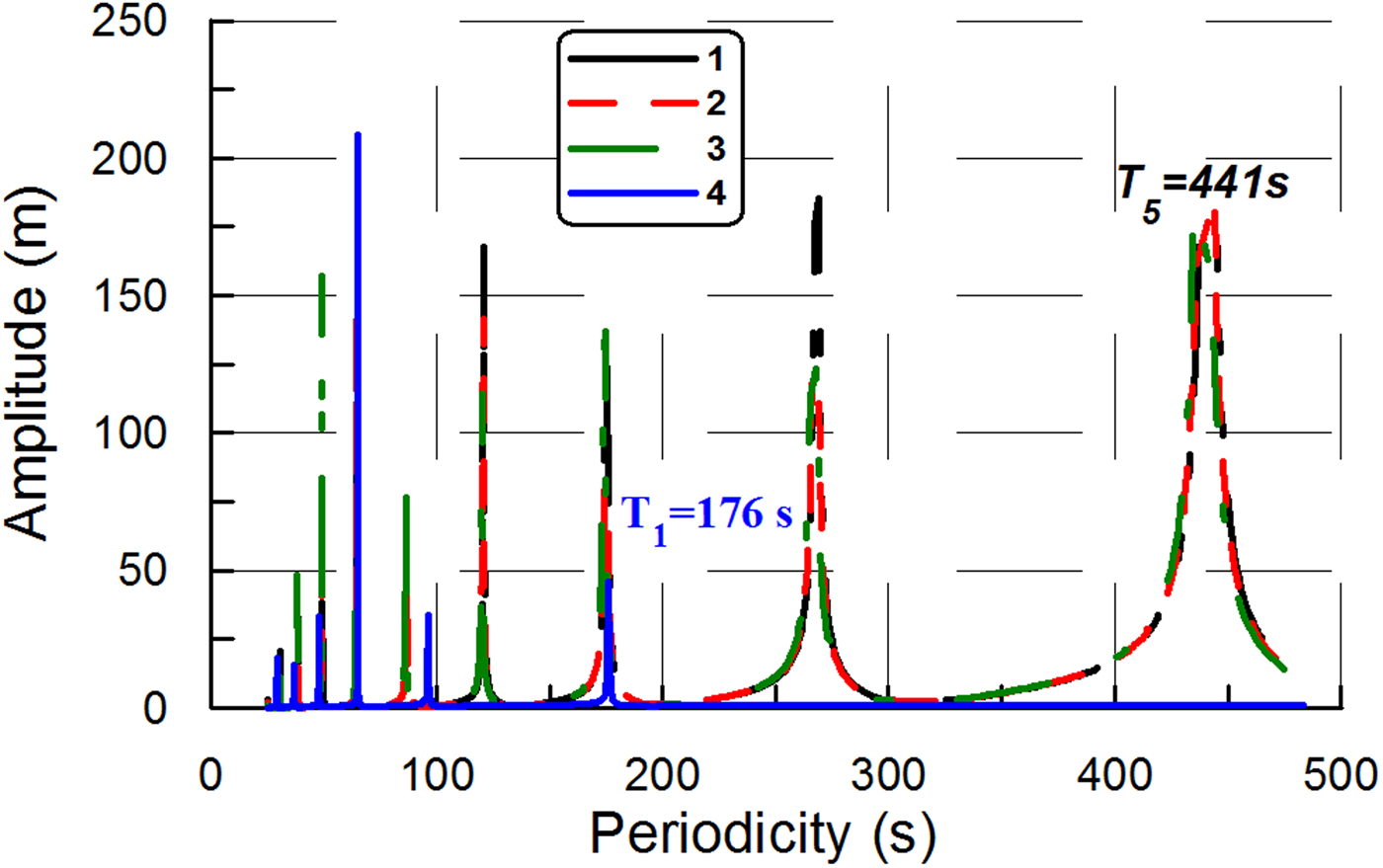
In Experiment C, the ice plate had only one fixed edge (at x = 0), while the other edges (at x = L, y 1 = 0, y 2 = B) were free. This is the special case of an ice-shelf that is also known as an ‘ice tongue’, which is unconfined by coastlines and simply flows across a single grounding line (e.g. Holdsworth and Glynn, Reference Holdsworth and Glynn1978). The water-layer depth was a constant value of 100 m. Ice tongue dimensions were L = 16 km, B = 800 m, H = 100 m. The aspect ratio γ was equal to 6.25 · 10−3 ( $\gamma = \; \sqrt {((d_0H)/L^2)} $). Figure 3 shows the amplitude spectra obtained in Experiment C for different values of α 1 and α 2 from Eqn (3). In fact, Figure 3 shows the part of the spectra, which begins with the resonant peak corresponding to eigenperiodicity T 5. The first eigenperiodicity T 1, derived from the modeled spectra, is ~2.03 · 104s. Moreover, Figure 3 shows the amplitude spectrum obtained in Experiment C with the Holdsworth and Glynn model (Holdsworth and Glynn, Reference Holdsworth and Glynn1978).
The amplitude spectra obtained in Experiment C. Ice tongue dimensions are L = 16 km, B = 800 m, H = 100 m. Sub-ice water depth is equal to 100 m. Aspect ratio γ ≈ 0.006. Сurves 1–3 are the amplitude spectra derived from the full model: 1 – α 1 = 1, α 2 = 0; 2 – α 1 = 0.8, α 2 = 0.2; 3 – α 1 = 0.6, α 2 = 0.4. Curve 4 is the amplitude spectrum obtained by the Holdsworth and Glynn model (Holdsworth and Glynn, Reference Holdsworth and Glynn1978). Young's modulus E = 9 GPa, Poisson's ratio ν = 0.33 (Schulson, Reference Schulson1999).
DISCUSSION
In Experiment A, the problem of free vibrations of the ice-shelf has the exact solution obtained in the thin-plate approximation (e.g. Landau and Lifshitz, Reference Landau and Lifshitz1986). In particular, the solution contains the plate eigenfrequencies that are expressed by Eqn (9). The expressions (9) show that the eigenfrequencies change proportionally to the ice-shelf thickness variations. These changes occur in agreement with the ratio (10).
The comparison of the eigenperiodicities obtained from Eqn (9) with the ones derived from the full model spectra shows the distinction of the ranges T belonging to (0, T 0] that contain all eigenvalues. In particular, the span of the range (0, T 0] in the full model is ~2.6 times higher than the span of the range obtained in the thin-plate approximation (Fig. 1). However, the spectra obtained by the full model also reveal the eigenvalues proportionality, which is described by the ratio (10).
Thus, Experiment A reveals the distinction between the thin-plate approximation and the full model. Moreover, this distinction stems from the equations that describe the elastic deformations of the plate, because the impact of the water layer is excluded in the Experiment A.
In Experiment B, the range that contains all eigenvalues of the full model is (0, 4.5 · 104s] (Fig. 2). In the Holdsworth and Glynn model (1978), the range is (0, 1138s]. These ranges contain both periodicities of ocean swell and infragravity waves, as well as the periodicities of tsunami waves. However, the interaction of the ice-shelf with the water layer yields a significant increase in the difference between the ranges computed by the full model and by the thin-plate approximation. In Experiment B, the span of the range (0, T 0] in the full model is ~40 times higher than the span of the range obtained in the thin-plate approximation.
In Experiment C, the range is (0, 2.03 · 104s] in the full model and the range is (0, 176 s] in the Holdsworth and Glynn model (1978) (Fig. 3). Thus, in the full model, the range includes periodicities of ocean swell, infragravity waves and tsunami waves. However, in the Holdsworth and Glynn model (1978), the range includes only periodicities of ocean swell and only part of periodicities of infragravity waves (50…176 s).
Thus, in Experiment C, the span of the range (0, T 0] in the full model is already ~115 times higher than the span obtained by the thin-plate approximation. This difference is ~3 times higher than the difference in Experiment B (115 and 40, respectively).
Essentially, fixing the lateral edge of the plate provides the decrease of the difference between the ranges in the thin-plate model (Holdsworth and Glynn, Reference Holdsworth and Glynn1978) and in the full model. However, this difference remains an order of magnitude larger than in Experiment A (40 and 2.6, respectively).
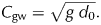
The velocity of long gravitational wave propagation is expressed as (e.g. Landau and Lifshitz, Reference Landau and Lifshitz1987)
 $$C_{{\rm gw}} = \sqrt {g\; d_0}. $$
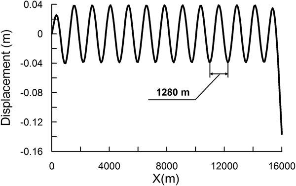
The assessment of the wavelength in the channel by Eqn (11) for d 0 = 100 m and T = 5 s gives the wavelength λ gw ≈ 156 m. However, the simulations show that for T = 5 s the wavelength in the channel bounded by the solid elastic plate (in Experiment C) is ~1280 m (Fig. 4).
Ice-shelf flexure along the central line obtained in Experiment C (α 1 = 1, α 2 = 0). Ice tongue dimensions are L = 16 km, B = 800 m, H = 100 m. Sub-ice water depth is equal to 100 m. The periodicity of the forcing is equal to 5 s.

For an explanation of this high value of the wavelength, we should account for the velocity of the shear wave propagation in the solid elastic plate. This velocity is defined as (e.g. Landau and Lifshitz, Reference Landau and Lifshitz1986)
 $$C_{\rm t} = \sqrt {\displaystyle{{E\;} \over {2\; \rho \; (1 + \nu )}}}. $$
Thus, we have C t ≈ 1928 m s−1, and this is significantly higher than the C gw = 31 m s−1 from Eqn (11). In particular, for T = 5 s the shear wavelength is λ t = C t T = 5784 m. Respectively, in Experiment C, the effective velocity of the wave propagation in the channel is about C eff = (λ/T) ≈ 256 m s−1 and C gw ≪ C eff ≪ C t. Thus, the condition, which allows to apply Eqn (2) ((d 0/λ) ≪ 1) is satisfied due to the rigidity of the ice-shelf even for relatively small values of the periodicity (T ≥ 2s).
It should be noted that the baseline amplitude provided by the model is the upper limit of the ice-shelf amplitude. This is because the viscosity of the fluid in the region below the ice-shelf is important and will ultimately limit resonant-like behavior. Moreover, the ice-shelf will ultimately begin to respond viscoelastically, and this too will limit resonant-like behavior (Reeh and others, Reference Reeh, Christensen, Mayer and Olesen2003; Walker and others, Reference Walker2013; Rosier and others, Reference Rosier, Gudmundsson and Green2014). With these two forms of dissipation (viscosity in the ocean and viscoelasticity in the ice-shelf), the real response of the system to forcing will be less than the baseline amplitude described by the modeled spectra.
CONCLUSIONS
The conclusions of the study presented here are summarized in the following list.
1) Essentially, the approximation of the boundary conditions employing the equations defined by Φi(U, V, W) in Eqn (3), i.e. when α 1 = 0, α 2 = 1, yields roughly the same spectrum as the case when α 1 = 1, α 2 = 0 (e.g. Fig. 1a). That is, the transition α 1 = 1, α 2 = 0 → α 1 = 0, α 2 = 1 does not excite complementary resonant peaks in the spectrum at a given range of periodicity T belonging to (t 1, T 0] (Fig. 1a). Essentially, we observe only the relatively small shift of the resonant peaks at a given range (t 1, T 0] (Fig. 1a).
2) Initially, the approximation given only by Φi(U, V, W) (α 1 = 0, α 2 = 1) was considered for achieving stability in the numerical solution. Thus, essentially, Φi(U, V, W) in Eqn (3) plays the role of the stabilizer. The approximation given only by Φi(U, V, W) suggests the integration of typical physical conditions into the basic momentum equations. In fact, the numerical experiments reveal that, despite a small difference between the output results (e.g. amplitude spectra and velocity profiles) and though the typical conditions are implied, they are not exactly satisfied in the model with α 1 = 0, α 2 = 1. For instance, if we have the condition σ xz = 0 at the ice front, then the shear stress will not equal zero at the front in the model with α 1 = 0, α 2 = 1. The approximation of the boundary conditions by Eqn (3) allows the basic/typical boundary conditions to be satisfied with a given accuracy (for instance, 90% at α 1 = 0.9, α 2 = 0.1), if the solution exists at a given α 1, α 2.
3) Despite the decrease of the aspect ratio in Experiment A, the superposition of the modeled spectra with the eigenfrequencies obtained from Eqn (9) was not observed. An explanation of the difference is suggested by considering the eigenvalues as the roots of the equation D(ω) = 0, in which D(ω) is the determinant of the matrix that resulted from discretization of the model. The determinant D(ω) is a polynomial expression and its roots depend on the number of equations in the model. Since the thin-plate approximation suggests a reduction of the number of equations in comparison with the full model (supposing that σ xz = σ yz = σ zz ≈ 0 in the plate), we can anticipate the decline of the set of roots, and therefore, the decrease of the array of eigenvalues in the thin-plate model. Thus, these results suggest that the future investigations of the problem should focus on the development and intercomparison of different full models.
4) The amplitude spectra determined using the approach derived in this study allow not only the specific resonant frequencies to be determined, but also the width of the resonant peaks that define ice-shelf/ocean response in a frequency ‘neighborhood’ surrounding each specific resonance frequency. Essentially, this width defines the probability of resonant-like amplitudes of the ice-shelf/ocean system's response to wave-forcing events, which typically span a wide neighborhood of frequencies that can contain the specific resonance frequency. The significance of the width is that, when it is larger, there is a higher probability of resonant-like motions to be excited from random wave events.
ACKNOWLEDGEMENTS
I thank the Scientific Editor (Douglas MacAyeal) and the reviewers of the journal for helpful discussion that allowed to improve this manuscript.



 Open access

