


1. Introduction
When a fluid-saturated porous layer undergoes bottom-up heating, it is prone to exhibit Rayleigh–Darcy convection (Horton & Rogers Reference Horton and Rogers1945; Lapwood Reference Lapwood1948; Graham & Steen Reference Graham and Steen1994). The main controlling parameter is the Rayleigh–Darcy number  $\textit {Ra}$, expressing the ratio of buoyancy to dissipative forces, and the resulting heat flux is characterized in terms of the Nusselt number, $\textit {Nu}$. The scaling of $\textit {Nu}$ with $\textit {Ra}$ in natural convection is traditionally described via power-law dependency, $\textit {Nu}\sim \textit {Ra}^{\alpha }$, although $\alpha$ may change as a result of the change in the structure of the convective flow. For instance, in Rayleigh–Bénard convection (He et al. Reference He, Funfschilling, Nobach, Bodenschatz and Ahlers2012; Lepot, Aumaître & Gallet Reference Lepot, Aumaître and Gallet2018; Zhu et al. Reference Zhu, Mathai, Stevens, Verzicco and Lohse2018; Wang, Zhou & Sun Reference Wang, Zhou and Sun2020), the general agreement is that $\alpha$ should gradually increase from about $1/3$ at moderate $\textit {Ra}$, to asymptotically approach a value of $1/2$, corresponding to the attainment of an ‘ultimate’ convection regime (Kraichnan Reference Kraichnan1962).
Classical theory suggests that the appropriate scaling in the ultimate regime of Rayleigh–Darcy convection should be linear (Malkus Reference Malkus1954; Howard Reference Howard1964). The main argument is that at high  $\textit {Ra}$, the interior part of the flow is perfectly mixed, and temperature gradients are confined to near-wall boundary layers whose thickness is $\delta \propto \textit {Ra}^{-1}$ (whereas in Rayleigh–Bénard convection $\delta \propto \textit {Ra}^{-1/3}$); hence $\textit {Nu} \propto \delta ^{-1} \propto \textit {Ra}$. Other more rigorous arguments have also been provided based on variational calculus, which show that linear scaling yields maximum heat transfer among all suitably energy-constrained flows (Otero et al. Reference Otero, Dontcheva, Johnston, Worthing, Kurganov, Petrova and Doering2004; Wen et al. Reference Wen, Dianati, Lunasin, Chini and Doering2012; Hassanzadeh, Chini & Doering Reference Hassanzadeh, Chini and Doering2014). This prediction is supported by existing numerical studies, mainly based on two-dimensional computations (Otero et al. Reference Otero, Dontcheva, Johnston, Worthing, Kurganov, Petrova and Doering2004; Hewitt, Neufeld & Lister Reference Hewitt, Neufeld and Lister2012; Wen et al. Reference Wen, Dianati, Lunasin, Chini and Doering2012; Wen, Corson & Chini Reference Wen, Corson and Chini2015; De Paoli, Zonta & Soldati Reference De Paoli, Zonta and Soldati2016) carried out in the range $\textit {Ra} \leqslant 10^5$. Three-dimensional simulations carried out in recent times up to $\textit {Ra}=2\times 10^4$ (Hewitt, Neufeld & Lister Reference Hewitt, Neufeld and Lister2014) also seem to support the establishment of a shifted linear variation of $\textit {Nu}$ with $\textit {Ra}$. However, given the limited range of $\textit {Ra}$ in which data are available, uncertainties remain regarding the actual establishment of the expected ultimate convection regime, and especially how it is reached starting from finite $\textit {Ra}$ (Hewitt Reference Hewitt2020).
The quest for the  $\textit {Nu}$ scaling in the high- $\textit {Ra}$ regime is crucial from a fundamental and also from an applied viewpoint, as the Rayleigh–Darcy model closely mimics flows in a number of geophysical applications, with special reference to geological $\textrm {CO}_2$ sequestration in deep saline aquifers (Hidalgo et al. Reference Hidalgo, Fe, Cueto-Felgueroso and Juanes2012; Huppert & Neufeld Reference Huppert and Neufeld2014; Riaz & Cinar Reference Riaz and Cinar2014; Emami-Meybodi et al. Reference Emami-Meybodi, Hassanzadeh, Green and Ennis-King2015; De Paoli Reference De Paoli2021). Real-life instances may exhibit $\textit {Ra}$ up to ${\sim }{ {O}}(10^5 \div 10^6)$, and small deviations from the expected ultimate linear scaling can produce large differences in the overall predicted transfer flux and in the corresponding cumulative time integral (Slim Reference Slim2014; De Paoli et al. Reference De Paoli, Zonta and Soldati2016; De Paoli, Zonta & Soldati Reference De Paoli, Zonta and Soldati2017). The goal of the present work is to investigate the high- $\textit {Ra}$ range of Rayleigh–Darcy convection, using a database of three-dimensional numerical simulations up to $\textit {Ra}=8\times 10^4$. Our aim is to extract reliable trends for the Nusselt number in a wide range of $\textit {Ra}$, and possibly to infer robust asymptotic estimates for the ultimate linear regime.
2. Methodology
We consider a fluid-saturated porous medium in a three-dimensional domain (see figure 1) with uniform porosity  $\phi$ and uniform permeability $\kappa$. The flow, which is incompressible and governed by the Darcy law, is characterized by an unstable density difference ( $\Delta \rho ^{*}$) induced by heating the flow from the bottom and cooling it from the top. Indicating by $x^*,z^*$ the horizontal directions, by $y^*$ the vertical direction (along which gravity acceleration $\boldsymbol {g}$ is directed) and by $\theta ^{*}$ the fluid temperature, the physical instance we consider corresponds to a fluid-saturated cubic volume with side length $h^{*}$ heated at the bottom, $\theta ^*(y^{*}=0)=\theta ^{*}_{max}$, and cooled at the top, $\theta ^*(y^{*}=h^{*})=\theta ^{*}_{min}$. The evolution of the temperature field is controlled by the advection–diffusion equation
 \begin{equation} \phi\frac{\partial \theta^{*}}{\partial t^{*}}+\boldsymbol{\nabla} \boldsymbol{\cdot}(\boldsymbol{u}^{*}\theta^{*}-\phi D \boldsymbol{\nabla}\theta^{*})=0 { ,} \end{equation}
where  $t^{*}$ is time, $\boldsymbol {u}^{*}=(u^{*},v^{*},w^{*})$ is the volume-averaged velocity field and $D$ is the thermal diffusivity, which is considered constant here. The superscript $^{*}$ is used to indicate dimensional variables. We assume that fluid density, $\rho ^{*}$, is a linear function of temperature,
 \begin{equation} \rho^{*}(\theta^{*})=\rho^{*}(\theta^{*}_{min})-\Delta\rho^{*}\frac{\theta^{*}-\theta^{*}_{min}}{\theta^{*}_{max}- \theta^{*}_{min}}{ ,} \end{equation}
with  $\Delta \rho ^{*}=\rho ^{*}(\theta ^{*}_{min})-\rho ^{*}(\theta ^{*}_{max})$. Assuming validity of the Boussinesq approximation (Landman & Schotting Reference Landman and Schotting2007; Zonta & Soldati Reference Zonta and Soldati2018), the flow field is fully described by the continuity and Darcy equations
 \begin{equation} \boldsymbol{\nabla}\boldsymbol{\cdot}\boldsymbol{u}^{*}=0,\quad \boldsymbol{u}^{*}=-\frac{\kappa}{\mu}\left(\boldsymbol{\nabla}P^{*}+\rho^{*}g \boldsymbol{j}\right) { ,} \end{equation}
with  $\mu$ the fluid viscosity (constant), $P^{*}$ the pressure and $\boldsymbol {j}$ the vertical unit vector. The walls are assumed to be impermeable and isothermal, and periodicity is assumed in the wall-parallel directions.
Sketch of the computational domain – a cube with side length  $h^*$ – used to study Rayleigh–Darcy convection. The flow is heated at the bottom, $\theta ^*(y^*=0)=\theta ^*_{{max}}$, and cooled at the top, $\theta ^*(y^*=h^*)=\theta ^*_{{min}}$, and boundaries in the $x^*$ and $z^*$ directions are assumed to be periodic. The gravity acceleration ( $\boldsymbol {g}$) points downwards. The temperature distribution $\theta ^*$ for the case $\textit {Ra}=1\times 10^4$ is also shown for illustrative purposes on the side boundaries and in a plane very close to the top boundary (i.e. at a distance of $50h^*/\textit {Ra}$ from the top boundary).

2.1. Dimensionless equations
Natural velocity and length scales for the system are the buoyancy velocity,  $V^{*}=g \Delta \rho ^{*} \kappa / \mu$, and the domain height, $h^{*}$, respectively. Using the set of dimensionless variables
 \begin{equation} \theta=\frac{\theta^{*}-\theta^{*}_{min}}{\theta^{*}_{max}-\theta^{*}_{min}} ,\quad t=\frac{t^{*}}{\phi h^{*}/V^{*}},\quad P=\frac{P^{*}}{\Delta \rho^{*}gh^{*}} , \end{equation}
and introducing the reduced pressure  $p^{*}$, we obtain the dimensionless form of the governing equations (2.1), (2.3a,b):
 \begin{gather} \frac{\partial \theta}{\partial t}+\boldsymbol{\nabla} \boldsymbol{\cdot} \left( {\boldsymbol{u}} \theta -\frac{1}{\textit{Ra}} \boldsymbol{\nabla} \theta\right)=0 ,\end{gather}
 \begin{gather} \boldsymbol{\nabla}\boldsymbol{\cdot}\boldsymbol{u}=0,\quad {\boldsymbol{u}}=-\left( \boldsymbol{\nabla} p -\theta \boldsymbol{j}\right) ,\end{gather}
where  $\textit {Ra}=g \Delta \rho ^{*} \kappa h^{*} / (\phi D \mu )=V^{*} h^{*} / (\phi D)$ is the Rayleigh–Darcy number. The wall boundary conditions for velocity and temperature then read as
 \begin{gather} v(y=0)=0,\quad \theta(y=0)=1, \end{gather}
 \begin{gather}v(y=1)=0,\quad \theta(y=1)=0. \end{gather}
 As previously mentioned, for the physical system investigated here, the buoyancy velocity  $V^{*}$ is a natural reference velocity scale (Fu, Cueto-Felgueroso & Juanes Reference Fu, Cueto-Felgueroso and Juanes2013; Wen et al. Reference Wen, Akhbari, Zhang and Hesse2018). At the same time, a possible reference length scale is the thickness of the porous layer, ${x}_{c}^{*}=h^*$ (convective scaling). However, an alternative choice for the reference length scale, which is perhaps more related to the physics of the phenomena under investigation, is ${x}_{d}^{*}=\phi D/V^{*}$ (diffusive–convective scaling). Note that ${x}^{*}_{d}$ represents the length over which advection and diffusion balance (Slim Reference Slim2014), and is independent of the physical domain thickness. When rescaled in the latter way, dimensions are bounded within the range ${x}^{*}/{x}_{d}^{*}\in [0,\textit {Ra}]$, and comparison between simulations at different $\textit {Ra}$ is easier. For this reason, lengths in this paper are rescaled with respect to $x_{d}^{*}$. Furthermore, introduction of this length scale also yields another interpretation of the Rayleigh–Darcy number, $\textit {Ra}={x}_{c}^{*}/{x}_{d}^{*}$, which may be regarded as the dimensionless height of the domain (Slim Reference Slim2014).
2.2. Computational details
The numerical simulations rely on the modified version of a second-order finite-difference incompressible flow solver, based on staggered arrangement of the flow variables (Orlandi Reference Orlandi2000), which has been extensively used for DNS of wall-bounded neutrally-buoyant and unstably-stratified turbulent flows (Pirozzoli Reference Pirozzoli2014; Pirozzoli et al. Reference Pirozzoli, Bernardini, Verzicco and Orlandi2017). The temperature transport equation is advanced in time by means of a hybrid third-order low-storage Runge–Kutta algorithm, whereby the convective terms are handled explicitly and the diffusive terms are handled implicitly, limited to the wall-normal direction. This approach guarantees that the total temperature variance is discretely preserved in the limit of inviscid flow. The pressure field in the forced Darcy equation is determined by solving the Poisson equation resulting from the divergence-free constraint,
 \begin{equation} \nabla^2 p = \frac{\partial \theta}{\partial y}, \end{equation}
with  $\partial p / \partial y = 0$ at walls to satisfy the impermeability condition, which is then fed into (2.6a,b). Fourier expansion along the horizontal periodic directions yields a system of tridiagonal equations in the wall-normal direction for each Fourier mode, which is then solved with standard highly efficient numerical techniques (Kim & Moin Reference Kim and Moin1985; Orlandi Reference Orlandi2000).
The mesh spacing in the wall-parallel directions was decided based on preliminary grid-resolution studies at low  $\textit {Ra}$ and inspection of the temperature spectra, to prevent any energy pile-up at the smallest resolved flow scales. Regarding the resolution in the wall-normal direction, we have followed the criterion that twenty points should be placed within the thermal boundary layer edge, identified through the peak location of the temperature variance, and grid points are clustered towards the walls using a hyperbolic tangent stretching function. Given the expected linear growth of the temperature gradients, the number of points in each coordinate direction was increased proportionally to $\textit {Ra}$. The time step is selected so that the CFL number is approximately unity for all the simulations herein reported. Preliminary calculations, carried out at $\textit {Ra} \leqslant 5\times 10^3$, have shown excellent agreement with the results of Hewitt et al. (Reference Hewitt, Neufeld and Lister2014).
3. Results
3.1. Heat transfer
We have carried out numerical simulations in the Rayleigh number range  $2.5\times 10^3<\textit {Ra}<8\times 10^4$. Note that, because of the time step restrictions, the simulation at $\textit {Ra}=8\times 10^4$ – using $6144\times 6144\times 2048$ grid points – is almost 4096 times more computationally expensive than the simulation at $\textit {Ra}=1\times 10^4$ – using $768\times 768\times 256$ grid points – hence the computational challenge is substantial. A summary of the main computational parameters is provided in table 1. The heat flux is quantified in terms of the Nusselt number $\textit {Nu}$, evaluated as the mean temperature gradient at the top and bottom boundaries,
 \begin{equation} \textit{Nu}=-\left \langle \frac{1}{2}\int_{0}^{1}\int_{0}^{1}\left.\frac{\partial \theta}{\partial y}\right\vert_{y=0}+\left.\frac{\partial \theta}{\partial y}\right\vert_{y=1} \,\text{d}x\,\text{d}z\right\rangle, \end{equation}
with angle brackets indicating time averaging.
Parameters of the main three-dimensional simulations performed in the present study. For each simulation, we report Rayleigh number  $\textit {Ra}$, grid resolution $N_{x}\times N_{z}\times N_{y}$, Nusselt number $\textit {Nu}$, and number of samples $N_{s}$ over which $\textit {Nu}$ is averaged (see appendix B for further details). Additional three-dimensional simulations (not listed here) have been performed at $\textit {Ra}=2.5\times 10^3, 5\times 10^3$.

In figure 2 we show the computed values of  $\textit {Nu}$ as a function of $\textit {Ra}$ (filled circles), compared with data available in the literature (open triangles, Hewitt et al. Reference Hewitt, Neufeld and Lister2014). Also shown in light grey is the high- $\textit {Ra}$ portion of the $(\textit {Ra},\textit {Nu})$ parameter space covered in previous three-dimensional numerical simulations. The dash-dot line in figure 2 corresponds to the prediction of Hewitt et al. (Reference Hewitt, Neufeld and Lister2014) based on fitting of lower- $\textit {Ra}$ data ( $\textit {Ra} \leqslant 2\times 10^4$), and amounting to a shifted linear variation, $\textit {Nu}=0.0096\textit {Ra} + 4.6$. As seen from figure 2, this fit overestimates our data by about $9\,\%$ at the highest $\textit {Ra}$; hence we believe that a different expression may be appropriate to more accurately characterize the trend towards the ultimate linear scaling.
Nusselt number as a function of the Rayleigh–Darcy number. Results obtained from the present numerical simulations are shown with filled circles, and the fitting curve,  $\textit {Nu}=0.0081\textit {Ra}+0.067 \textit {Ra}^{0.61}$, is shown as a black solid line. Results obtained in previous simulations by Hewitt et al. (Reference Hewitt, Neufeld and Lister2014) (open triangles) and the extrapolated shifted linear scaling (blue dash-dotted line) are shown for comparison. The high- $\textit {Ra}$ portion of the $(\textit {Ra},\textit {Nu})$ parameter space covered by previous investigations is rendered by the light grey rectangle.

In figure 3 we thus show the compensated Nusselt number  $\textit {Nu}/\textit {Ra}$, for a collection of current and previous numerical data obtained in three-dimensional (Hewitt et al. Reference Hewitt, Neufeld and Lister2014) and two-dimensional (Hewitt et al. Reference Hewitt, Neufeld and Lister2012; Wen et al. Reference Wen, Corson and Chini2015; De Paoli et al. Reference De Paoli, Zonta and Soldati2016) domains. According to the prediction of Hewitt et al. (Reference Hewitt, Neufeld and Lister2014), the asymptotic value $\textit {Nu}/\textit {Ra}=0.0096$ should be reached for $\textit {Ra} \gtrsim 10^5$. Our data (filled circles) for $\textit {Ra}>2\times 10^4$ fall well below that prediction, showing no clear evidence for inception of an ultimate regime. An improved prediction for the pre-asymptotic regime can be constructed by fitting the numerical data and relying on the compelling evidence that the asymptotic scaling should be linear (Hewitt Reference Hewitt2020). Data fitting then results in a functional representation of the type
 \begin{equation} \textit{Nu}/\textit{Ra}=0.0081+0.067\textit{Ra}^{-0.39} , \end{equation}
which amounts to linear dependence of  $\textit {Nu}$ over $\textit {Ra}$ augmented with a sublinear corrective term, shown as a black solid line in figure 3. Compared with previous estimates, this correlation yields good prediction of $\textit {Nu}$ over a much larger range of $\textit {Ra}$, starting at $\textit {Ra} \sim 2.5\times 10^3$, with error no larger than $1.5\,\%$. Extrapolation to higher $\textit {Ra}$ than reached in the present computational campaign would yield the asymptotic scaling
 \begin{equation} \textit{Nu} = 0.0081 \textit{Ra} , \end{equation}
in the ultimate regime. Based on our data, we expect that to have deviations of less than  $5\,\%$ from the ultimate regime, $\textit {Ra}$ in excess of $5\times 10^5$ is needed. At those huge Rayleigh numbers, which closely represent the case of geological $\textrm {CO}_{2}$ sequestration in deep saline aquifers, differences between the current prediction and previous predictions of Hewitt et al. (Reference Hewitt, Neufeld and Lister2014) would be as large as ${\sim }16\,\%$. These findings are contrasted in figure 3 with the case of two-dimensional flow, for which the data generally support $\textit {Nu} \approx 0.0069 \textit {Ra} + 2.75$, as suggested by Hewitt et al. (Reference Hewitt, Neufeld and Lister2012), and attainment of a linear trend at $\textit {Ra} \sim 3\times 10^4$. Hence, extrapolation of our results yields the prediction that in the ultimate regime the Nusselt number should be larger by about $18\,\%$ in the three-dimensional than in the two-dimensional case.
Compensated Nusselt number as a function of the Rayleigh–Darcy number,  $\textit {Ra}$. Results obtained from the present numerical simulations, which we have run in three-dimensional and two-dimensional domains, are shown by filled circles ( $\bullet$) and diamonds ( $\blacklozenge$), respectively. For comparison purposes, a collection of previous data obtained in both two-dimensional domains (Hewitt et al. Reference Hewitt, Neufeld and Lister2012; De Paoli et al. Reference De Paoli, Zonta and Soldati2016; Wen et al. Reference Wen, Corson and Chini2015) ( $\square$, $\triangledown$ and $\triangleright$, respectively) and three-dimensional domains (Hewitt et al. Reference Hewitt, Neufeld and Lister2014) ( $\triangle$) is also shown, with open symbols. The black solid line denotes the best fit of our three-dimensional data, as from (3.2), and the blue solid line the shifted linear scaling $\textit {Nu}/\textit {Ra}=0.096+4.6/\textit {Ra}$ predicted by Hewitt et al. (Reference Hewitt, Neufeld and Lister2014). The scaling law $\textit {Nu}/\textit {Ra}=0.0069+2.75/\textit {Ra}$ proposed by Hewitt et al. (Reference Hewitt, Neufeld and Lister2012) for the two-dimensional case is shown with a solid red line. The asymptotic predictions for each scaling law are reported as dashed lines.

3.2. Flow structure
It is reasonable to expect that the heat transfer behaviour just discussed is reflected in the behaviour of the flow structure. We characterize the flow structure focusing on its signature in the near-boundary region where the contribution of both diffusion-driven and buoyancy-driven mechanisms is important. An estimate of the location at which diffusion and buoyancy are both important is given by the temperature boundary layer thickness,  $\delta$, which, in Rayleigh–Darcy convection, is
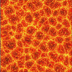
  $\delta \sim 30/\textit {Ra}$ (see Otero et al. (Reference Otero, Dontcheva, Johnston, Worthing, Kurganov, Petrova and Doering2004), Hewitt et al. (Reference Hewitt, Neufeld and Lister2012), and also appendix A of the present manuscript). Accordingly, in figure 4 we show the temperature distributions in a horizontal plane at $y=50/\textit {Ra}$ from the bottom boundary. Indication of the domain size in diffusive–convective units, $x^*_d$, for the simulations at lower $\textit {Ra}$ is given by the white boxes in panel (a). The complex flow pattern near the boundary, which appears to be still developing at $\textit {Ra}<2\times 10^4$, seems to attain a roughly self-similar structure at larger $\textit {Ra}$. Hence, in the following we will mostly refer to the $S_8$ simulation, since the flow features we wish to discuss are emphasized at that value of $\textit {Ra}$.
Temperature distribution in a plane close to the bottom boundary  $(x,y=50/\textit {Ra},z)$, for simulations $S_8$ (a), $S_4$ (b), $S_2$ (c) and $S_1$ (d). The domain size is also explicitly indicated in diffusive–convective units in each panel. Indication of the domain size – rescaled using the diffusive–convective length scale $x^*_d$ – for the simulations at lower $\textit {Ra}$ is given in panel (a) by the white boxes. The size of the superstructures, estimated as $\lambda _i=2{\rm \pi} \textit {Ra}/k_i$ with $k_i/\textit {Ra}$ defined as in figure 5, is also shown in each panel (black bars).

In figure 4 (and in particular in panel (a)) we clearly observe the presence of thin bright filaments which appear to be connected in a quasi-regular pattern of cells (Fu et al. Reference Fu, Cueto-Felgueroso and Juanes2013; Amooie, Soltanian & Moortgat Reference Amooie, Soltanian and Moortgat2018). These filaments correspond to regions where high-temperature fluid protrudes from the boundary, and are produced by tiny instabilities of the thermal boundary layer. Those are the three-dimensional counterpart of the protoplumes observed in previous two-dimensional studies (Hewitt et al. Reference Hewitt, Neufeld and Lister2012; Wen et al. Reference Wen, Corson and Chini2015; De Paoli et al. Reference De Paoli, Zonta and Soldati2016), and define the perimeter of rather homogeneous (dark) regions produced by downwelling motions (downwashes) of cold fluid towards the bottom boundary (see also the vertical slices shown in appendix A and comments therein). After impinging on the boundary, these downwashes spread horizontally and interact with the rising protoplumes, determining a dynamic pattern, in which some of the protoplumes eventually cluster into specific regions – thicker bright ridges (see figure 4a) – that define the boundaries of seemingly regular superstructures. These ‘supercells’, which encapsulate larger ensembles of smaller cells, have shape and dynamics recalling those of classical Rayleigh–Bénard turbulence (Stevens et al. Reference Stevens, Blass, Zhu, Verzicco and Lohse2018; Krug, Lohse & Stevens Reference Krug, Lohse and Stevens2020) or those of solar granules in the Sun's photosphere (Bahng & Schwarzschild Reference Bahng and Schwarzschild1961; Miesch Reference Miesch2005; Rieutord & Rincon Reference Rieutord and Rincon2010; Witze Reference Witze2020) (see also animations in the supplementary movies available at https://doi.org/10.1017/jfm.2020.1178 for a time-resolved rendering of the supercells). The size of the supercells  $\lambda _i$, as inferred from the analysis of the wavenumber spectra (see figure 5 and the corresponding discussion), can be appreciated in figure 4. Since at large $\textit {Ra}$ the size of the supercells, which is approximately one-tenth of the box side length for simulation $S_8$ – see figure 4(a) – does not seem to evolve once the simulation has reached the steady state, we are keen to attribute to them an important role in the overall heat transfer mechanisms. At the same time, an important role is played by the smaller cells enclosed by supercells. Previous qualitative observations show a complex network of structures composed of small cells hierarchically nesting into supercells. To determine the size of such supercells, we use the time-averaged wavenumber power spectrum of the temperature signal, $P(k)$, which we obtain by taking the two-dimensional Fourier transform of the temperature field in a horizontal plane located near the boundary (such as the one sketched in figure 4a).
Power spectra  $k_{r}P(k_{r})$ (solid lines and symbols) of temperature distribution near the boundary (sampled at the location $y=50/\textit {Ra}$, as in figure 4), shown as a function of the radial wavenumber $k_{r}=\sqrt {k_{x}^{2}+k_{z}^{2}}$, for all $\textit {Ra}$ considered here. Results of the $S_3$ simulation are omitted for ease of reading. In the inset of the figure we plot the power spectra of the temperature distribution at the centre (midplane) of the domain. Labels $k_i/\textit {Ra}$ and $k'_i/\textit {Ra}$ indicate the peaks of the spectra. The corresponding wavenumber is explicitly reported in the main panel.

In figure 5, we show  $k_rP(k_r)$ as a function of the normalized radial wavenumber $k_r/\textit {Ra}$, where $k_r=\sqrt {k_x^2+k_z^2}$, and $k_x$ and $k_z$ are the wavenumbers along $x$ and $z$, respectively. Results of the $S_3$ simulation are not shown, for better readability. For all considered values of $\textit {Ra}$, a sharp peak occurs at low wavenumbers, which clearly characterizes the size of the supercells. The wavenumber at which this peak occurs, labelled with $k_i/\textit {Ra}$ in figure 5 (where $i$ refers to the simulation number as in table 1, i.e. $i=1, 2, 4, 8$), decreases for increasing $\textit {Ra}$, thus indicating growth of the supercells with $\textit {Ra}$. Measurements of the temperature power spectrum at the midplane of the domain (inset of figure 5) is also characterized by the presence of sharp peaks (labelled as $k'_i/\textit {Ra}$), which in this case are due to large megaplumes developing in the interior part of the domain (Hewitt et al. Reference Hewitt, Neufeld and Lister2012; Hewitt, Neufeld & Lister Reference Hewitt, Neufeld and Lister2013; De Paoli et al. Reference De Paoli, Zonta and Soldati2016; Hewitt & Lister Reference Hewitt and Lister2017).
Direct comparison with the spectra near the boundary shows close coincidence of the spectral peaks, thus clearly indicating that supercells at the boundary are the footprint of the megaplumes that dominate the interior part of the flow. At larger  $k_{r}$, the spectrum near the boundary features a local minimum, followed by rapid increase. Such increase, which is not present in the spectrum at the domain centre, is naturally associated with the small-scale protoplumes populating the region near the boundary (see the small filaments in figure 4).
4. Conclusions
We have reported results of numerical simulation of Rayleigh–Darcy convection inside a cubic porous layer up to Rayleigh–Darcy number  $\textit {Ra}=8\times 10^4$. Exploiting the numerical dataset we show that the Nusselt number variation at sufficiently high $\textit {Ra}$ can be approximately expressed as $\textit {Nu}=0.0081\textit {Ra}+0.067\textit {Ra}^{0.61}$, with error bar no larger than $1.5\,\%$. Extrapolation of this prediction to the ultimate regime, which we expect to set in at $\textit {Ra} \gtrsim 5\times 10^5$, yields the asymptotic scaling $\textit {Nu}=0.0081\textit {Ra}$ – almost $16\,\%$ less than inferred in previous studies, and exceeding by about $18\,\%$ the Nusselt number found in two-dimensional simulations. We have further characterized the complex flow structure near the boundaries, which consists of small flow cells hierarchically nesting into supercells, and we have shown evidence that the supercells at the boundary are the footprint of megaplumes dominating the interior part of the flow. We believe that it would be possible to conduct direct investigations of the ultimate convective regime to check our extrapolations, by running a simulation at $\textit {Ra} \simeq 5\times 10^5$. However, we estimate a cost for this simulation of approximately 2 billion CPU hours, well beyond present-day capabilities.
Supplementary movies
Supplementary movies are available at https://doi.org/10.1017/jfm.2020.1178.
Acknowledgements
We are grateful to the CINECA supercomputing centre (under the grants ISCRA IsB20–3DSIMCON and PRACE Pra19-4938) and the Vienna Scientific Cluster (VSC) for generous allowance of computational resources. We also acknowledge Dr D. Hewitt and Dr B. Wen for providing data from Hewitt et al. (Reference Hewitt, Neufeld and Lister2012, Reference Hewitt, Neufeld and Lister2014) and Wen et al. (Reference Wen, Corson and Chini2015), respectively.
Funding
S.P. and F.Z. gratefully acknowledge financial support from the ERASMUS+ project 29415-EPP–1–2014–1–IT–EPPKA3–ECHE between TU Wien and La Sapienza University. The authors acknowledge financial support from the TU Wien University Library through its Open Access Funding Program.
Declaration of interests
The authors report no conflict of interest.
Appendix A. Structure of the flow in a vertical plane
In figure 6 we show the temperature distribution in a vertical  $(z,y)$ plane located at $x=1/2$. A close-up view of the temperature field near the boundary is also offered to exhibit the thickness of the thermal boundary layer, which, scaling as $\delta \sim 1/\textit {Ra}$, would otherwise be too small to be observed. Consistently with previous two- and three-dimensional studies (Hewitt et al. Reference Hewitt, Neufeld and Lister2012, Reference Hewitt, Neufeld and Lister2014; Wen et al. Reference Wen, Corson and Chini2015; De Paoli et al. Reference De Paoli, Zonta and Soldati2016), we observe that small fingers of light fluid emerge from the bottom boundary and move upwards, and correspondingly small fingers of heavy fluid emerge from the top boundary and move downwards. The small fingers then merge to form megaplumes (large columnar structures that dominate the core region of the flow) which, under the vigorous action of buoyancy, increase their vertical velocity and reach the opposite boundary. Upon impact with the boundary, the megaplumes are deflected and create the complex flow patterns analysed in detail in the main body of the present manuscript. As expected, the strength and persistence of the megaplumes increase with increasing $\textit {Ra}$.
Temperature distribution from the simulations  $S_1$ (a,b) and $S_8$ (c,d) in a vertical slice located at $x=1/2$. The dimensionless domain size in diffusive–convective units is indicated. A close-up view of the near-wall region, indicated with black squares in panels (a,c), is shown in panels (b,d).

Appendix B. Evaluation of the Nusselt number
To estimate the averaged Nusselt number, we first run each simulation (starting from a still fluid, plus random perturbations) until the initial transient is finished. From that time, labelled as  $t_{ss}$, the Nusselt number oscillates around a statistically steady value. In figure 7, we show the time evolution of the Nusselt number, $\textit {Nu}(t)$, over a specific time window after $t_{ss}$, for the main simulations herein performed. $\textit {Nu}(t)$ is observed to oscillate within $1\,\%$ to $3\,\%$ of the mean value (indicated by the dashed line). In particular, larger values of $\textit {Ra}$ correspond to lower relative amplitude of the fluctuations. The time-averaged Nusselt number (reported in table 1) is computed over a time window corresponding to 128, 64, 16, 8 and 4 dimensionless time units for $S_1$, $S_2$, $S_3$, $S_4$ and $S_8$, respectively. Naturally, the duration of the time window, $\Delta t=t-t_{ss}$, over which statistics are evaluated is less at the largest $\textit {Ra}$. However, it is important to point out that the Nusselt number is not only averaged in time, but also in space (along $x$ and $z$) over the entire wall surface, which increases the size of the ensemble over which statistics are evaluated. The effective number of samples, $N_{s}$, used to estimate the Nusselt number (and also reported in table 1) is here defined as $N_{s}=N_x\times N_z\times N_T$, where $N_T$ is the time interval (expressed in dimensionless convective units, i.e. turnover times) over which statistics are performed (starting from $t_{ss}$). Once the averaged value of the Nusselt number is estimated, we determine the best-fit scaling as in (3.2), yielding prediction error of no more than $1.5\,\%$, for $\textit {Ra} \geqslant 2.5 \times 10^3$.
Time evolution of instantaneous horizontally-averaged Nusselt number.  $\textit {Nu}$ is shown for simulations $S_1$ (a), $S_2$ (b), $S_3$ (c), $S_4$ (d) and $S_8$ (e). The behaviour of $\textit {Nu}(t)$ is reported for a portion of the simulation, after the steady state is achieved (the beginning of the steady-state regime is indicated by $t=t_{ss}$). We observe that $\textit {Nu}(t)$ (solid line) oscillates within $1\,\%$ to $3\,\%$ of the mean value (dashed line). For all simulations, $\textit {Nu}(t)$ is shown in the range corresponding to ${\pm }10\,\%$ of the time-averaged value. Since each point of the $\textit {Nu}(t)$ curve is the result of a space average (over the entire top and bottom wall), the larger $\textit {Ra}$ is, the larger the number of points over which the space average is evaluated, and so the lower the amplitude of the fluctuations.


 Open access