








1. Introduction
During the past decade, gas transfer across the air–water interface has received increasing interest because of its importance to the global greenhouse gas budget. At the air–water interface, heat and gas fluxes are dominated by molecular diffusion, which can be enhanced significantly by convective mixing. In nature, three sources of near-surface convective mixing can be identified. The first and most studied one is mixing by wind-shear-induced turbulence at the water surface. The second is turbulence generated at the bottom of a stream or by ocean currents that subsequently diffuses upwards to the surface where it enhances turbulent mixing. The third and least studied mechanism is due to a buoyant-convective instability, which is responsible for mixing during low-wind-speed conditions. In the ocean, free convection due to buoyant instabilities is often caused by vertical temperature and/or salinity gradients. This free convection induces near-surface turbulence, which enhances the exchange of heat and greenhouse gases (in particular carbon dioxide) between the atmosphere and the oceans.
Wind-shear-induced mixing has attracted significant attention because turbulence introduced immediately at the water surface is a very effective mechanism for promoting gas transfer. Especially larger wind speeds can induce significant wave growth and wave breaking, which further aid the mixing process (MacIntyre et al. Reference MacIntyre, Flynn, Jellison and Romero1999). Hence, in most cases the predictive estimation of heat and greenhouse gas fluxes only takes wind shear into account, which often results in an over- or under-prediction of the actual gas flux, especially in low-wind conditions (e.g. Nightingale et al. Reference Nightingale, Malin, Law, Watson, Liss, Liddicoat, Boutin and Upstill-Goddard2000; Crusius & Wanninkhof Reference Crusius and Wanninkhof2003; Smith et al. Reference Smith, Ho, Law, McGregor, Popinet and Schlosser2011).
Sheltered inland water bodies and equatorial ocean regions are examples of regions with low-wind-speed conditions that typically have large air–water $\text{CO}_{2}$
concentration gradients. These regions contribute significantly to the global
$\text{CO}_{2}$
concentration gradients. These regions contribute significantly to the global $\text{CO}_{2}$
budget (Feely et al.
Reference Feely, Boutin, Cosca, Dandonneau, Etcheto, Inoue, Ishii, Le Quere, Mackey and McPhaden2002), both as a major source of climatically important gases (in lakes and reservoirs: Cole et al.
Reference Cole, Prairie, Caraco, McDowell, Tranvik, Striegl, Duarte, Kortelainen, Downing and Middelburg2007; MacIntyre et al.
Reference MacIntyre, Jonsson, Jansson, Aberg, Turney and Miller2010) as well as a major sink for
$\text{CO}_{2}$
budget (Feely et al.
Reference Feely, Boutin, Cosca, Dandonneau, Etcheto, Inoue, Ishii, Le Quere, Mackey and McPhaden2002), both as a major source of climatically important gases (in lakes and reservoirs: Cole et al.
Reference Cole, Prairie, Caraco, McDowell, Tranvik, Striegl, Duarte, Kortelainen, Downing and Middelburg2007; MacIntyre et al.
Reference MacIntyre, Jonsson, Jansson, Aberg, Turney and Miller2010) as well as a major sink for $\text{CO}_{2}$
(in the equatorial ocean: Ishii et al.
Reference Ishii, Feely, Rodgers, Park, Wanninkhof, Sasano, Sugimoto, Cosca, Nakaoka and Telszewski2014). MacIntyre et al. (Reference MacIntyre, Jonsson, Jansson, Aberg, Turney and Miller2010) showed that for wind speeds lower than
$\text{CO}_{2}$
(in the equatorial ocean: Ishii et al.
Reference Ishii, Feely, Rodgers, Park, Wanninkhof, Sasano, Sugimoto, Cosca, Nakaoka and Telszewski2014). MacIntyre et al. (Reference MacIntyre, Jonsson, Jansson, Aberg, Turney and Miller2010) showed that for wind speeds lower than $5~\text{m}~\text{s}^{-1}$
the gas transfer velocity
$5~\text{m}~\text{s}^{-1}$
the gas transfer velocity $K_{L}$
is independent of wind speed and the buoyancy-driven flux dominates. In the ocean Soloviev & Klinger (Reference Soloviev, Klinger, Steele, Thorpe and Turekain2001) and Rutgersson, Smedman & Sahlee (Reference Rutgersson, Smedman and Sahlee2011) have reported that in low-wind-speed conditions buoyant convection due to surface cooling contributes significantly to the surface gas exchange.
$K_{L}$
is independent of wind speed and the buoyancy-driven flux dominates. In the ocean Soloviev & Klinger (Reference Soloviev, Klinger, Steele, Thorpe and Turekain2001) and Rutgersson, Smedman & Sahlee (Reference Rutgersson, Smedman and Sahlee2011) have reported that in low-wind-speed conditions buoyant convection due to surface cooling contributes significantly to the surface gas exchange.
Another important example of buoyant-convective mixing in nature is the absorption of oxygen into lakes or reservoirs driven by surface cooling. At night, the gas-saturated surface layer is cooled and becomes slightly heavier than the water underneath. Small fluctuations may trigger an instability, resulting in cold oxygen-saturated surface water plunging down and being replaced by warmer unsaturated fluid from below. This process results in the re-aeration of sheltered bodies of water, which is needed for biodegradation of organic wastes.
In order to improve current models used for the prediction of gas fluxes, there is a need for a detailed understanding of buoyant-convective mixing processes. To explore the effect of these processes requires an in-depth investigation of the interaction between the near-surface flow field and the interfacial mass flux, which – in contrast to the relatively abundant empirical quantification of the gas transfer velocity – is currently still lacking.
The gas flux across the air–water interface $j_{z}$
is defined by
$j_{z}$
is defined by
 $$\begin{eqnarray}\displaystyle j_{z}=K_{L}(C_{s}-C_{b}), & & \displaystyle\end{eqnarray}$$
where $K_{L}$
is the transfer velocity,
$K_{L}$
is the transfer velocity, $C_{s}$
is the saturated gas concentration at the interface and
$C_{s}$
is the saturated gas concentration at the interface and $C_{b}$
is the gas concentration in the bulk. The transfer velocity
$C_{b}$
is the gas concentration in the bulk. The transfer velocity $K_{L}$
is governed by the complex interaction of molecular diffusion and turbulent transport on either side of the surface and also depends on surface conditions as well as the chemical reactivity of the dissolved gas. At a constant temperature Henry’s law states that at equilibrium the solubility of an atmospheric gas in water increases linearly with its partial pressure in air,
$K_{L}$
is governed by the complex interaction of molecular diffusion and turbulent transport on either side of the surface and also depends on surface conditions as well as the chemical reactivity of the dissolved gas. At a constant temperature Henry’s law states that at equilibrium the solubility of an atmospheric gas in water increases linearly with its partial pressure in air, $p_{a}$
, so that
$p_{a}$
, so that $C_{s}=p_{a}/H$
, where
$C_{s}=p_{a}/H$
, where $H$
denotes Henry’s constant. (Note that the evaluation of
$H$
denotes Henry’s constant. (Note that the evaluation of $C_{s}$
is important in order to accurately determine
$C_{s}$
is important in order to accurately determine $j_{z}$
.) The partition coefficient of a gas between the atmosphere and water is defined by
$j_{z}$
.) The partition coefficient of a gas between the atmosphere and water is defined by $\mathscr{K}=C_{g}/C_{s}$
, where
$\mathscr{K}=C_{g}/C_{s}$
, where $C_{g}$
is the gas concentration in the air. (For an ideal gas,
$C_{g}$
is the gas concentration in the air. (For an ideal gas, $\mathscr{K}$
is related to
$\mathscr{K}$
is related to $H$
by
$H$
by $\mathscr{K}=H/RT$
, where
$\mathscr{K}=H/RT$
, where $R$
is the gas constant and
$R$
is the gas constant and $T$
is the temperature.) As shown by Liss (Reference Liss1973), the total transfer velocity
$T$
is the temperature.) As shown by Liss (Reference Liss1973), the total transfer velocity $K_{L}$
can be related to the individual gas transfer coefficients (
$K_{L}$
can be related to the individual gas transfer coefficients ( $k_{L}$
and
$k_{L}$
and $k_{g}$
for the liquid and gas phase, respectively) by
$k_{g}$
for the liquid and gas phase, respectively) by
 $$\begin{eqnarray}\frac{1}{K_{L}}=\frac{1}{k_{L}}+\frac{1}{\mathscr{K}k_{g}}.\end{eqnarray}$$
This ‘resistance-in-series model’ shows that the ratio $k_{L}/\mathscr{K}k_{g}$
determines whether the concentration boundary layer on the air or on the water side controls the gas transfer process (offers more resistance). With increasing solubility (which may be caused by a decreasing temperature) the control of the atmospheric gas transfer process will gradually shift to the air side. Environmentally important gases typically have a low (
$k_{L}/\mathscr{K}k_{g}$
determines whether the concentration boundary layer on the air or on the water side controls the gas transfer process (offers more resistance). With increasing solubility (which may be caused by a decreasing temperature) the control of the atmospheric gas transfer process will gradually shift to the air side. Environmentally important gases typically have a low ( $\text{O}_{2}$
, CO, NO) to moderate (
$\text{O}_{2}$
, CO, NO) to moderate ( $\text{CO}_{2}$
) solubility. Because of this and their significantly lower diffusivities in water than in air (hence
$\text{CO}_{2}$
) solubility. Because of this and their significantly lower diffusivities in water than in air (hence $k_{L}\ll k_{g}$
), for such gases
$k_{L}\ll k_{g}$
), for such gases $k_{L}/\mathscr{K}k_{g}$
is small and their transfer process at the air–water interface is concentrated in an extremely thin boundary layer (
$k_{L}/\mathscr{K}k_{g}$
is small and their transfer process at the air–water interface is concentrated in an extremely thin boundary layer ( $10{-}1000~{\rm\mu}\text{m}$
) on the liquid side (see Liss Reference Liss1973; Jähne & Haussecker Reference Jähne and Haussecker1998). It should be noted that
$10{-}1000~{\rm\mu}\text{m}$
) on the liquid side (see Liss Reference Liss1973; Jähne & Haussecker Reference Jähne and Haussecker1998). It should be noted that $\text{CO}_{2}$
is a chemically reactive gas in water and can be hydrated at the water surface, which chemically enhances the transfer velocity (see Wanninkhof & Knox Reference Wanninkhof and Knox1996).
$\text{CO}_{2}$
is a chemically reactive gas in water and can be hydrated at the water surface, which chemically enhances the transfer velocity (see Wanninkhof & Knox Reference Wanninkhof and Knox1996).
The small size of the concentration boundary layer on the liquid side makes it extremely difficult to carry out direct measurements of the diffusive ( $-D\,\partial C/\partial z$
) and turbulent (
$-D\,\partial C/\partial z$
) and turbulent ( $w^{\prime \prime }C^{\prime \prime }$
) vertical mass fluxes, where
$w^{\prime \prime }C^{\prime \prime }$
) vertical mass fluxes, where $C$
is the concentration of the solute,
$C$
is the concentration of the solute, $w$
is the velocity in the vertical (
$w$
is the velocity in the vertical ( $z$
) direction and
$z$
) direction and $D$
is the molecular diffusion coefficient (double primes denoting fluctuations with respect to statistical averages). Together, the diffusive and turbulent mass fluxes determine the total mass flux
$D$
is the molecular diffusion coefficient (double primes denoting fluctuations with respect to statistical averages). Together, the diffusive and turbulent mass fluxes determine the total mass flux $j_{z}$
in the vertical direction. The mass flux averaged over horizontal planes is a function of depth (
$j_{z}$
in the vertical direction. The mass flux averaged over horizontal planes is a function of depth ( $z$
) and time (
$z$
) and time ( $t$
), as given by
$t$
), as given by
 $$\begin{eqnarray}\displaystyle \langle \,j_{z}\rangle (z,t)=-\!\left[D\frac{\partial \langle C\rangle }{\partial z}-\langle w^{\prime \prime }C^{\prime \prime }\rangle \right]. & & \displaystyle\end{eqnarray}$$
Because it is difficult to perform measurements inside the tiny layer of gas-saturated fluid at the water surface, previous measurements focused mainly on measuring the overall transfer velocity $K_{L}$
. Equations (1.1) and (1.3) imply that to gain a fundamental understanding of the overall transfer velocity
$K_{L}$
. Equations (1.1) and (1.3) imply that to gain a fundamental understanding of the overall transfer velocity $K_{L}$
it is necessary to resolve both the diffusive and turbulent mass transfer terms.
$K_{L}$
it is necessary to resolve both the diffusive and turbulent mass transfer terms.
Numerous studies proposed empirical models which relate the transfer velocity $K_{L}$
to global parameters such as the bulk velocity of a stream, the bottom slope and friction (e.g. Tsivoglou & Wallace Reference Tsivoglou and Wallace1972; Chu & Jirka Reference Chu and Jirka2003). As mentioned above, for the case where buoyancy is likely to dominate,
$K_{L}$
to global parameters such as the bulk velocity of a stream, the bottom slope and friction (e.g. Tsivoglou & Wallace Reference Tsivoglou and Wallace1972; Chu & Jirka Reference Chu and Jirka2003). As mentioned above, for the case where buoyancy is likely to dominate, $K_{L}$
has been mostly related to wind shear alone (e.g Liss & Slater Reference Liss and Slater1974; Nightingale et al.
Reference Nightingale, Malin, Law, Watson, Liss, Liddicoat, Boutin and Upstill-Goddard2000; Crusius & Wanninkhof Reference Crusius and Wanninkhof2003). This has led to considerable inaccuracies in the estimation of
$K_{L}$
has been mostly related to wind shear alone (e.g Liss & Slater Reference Liss and Slater1974; Nightingale et al.
Reference Nightingale, Malin, Law, Watson, Liss, Liddicoat, Boutin and Upstill-Goddard2000; Crusius & Wanninkhof Reference Crusius and Wanninkhof2003). This has led to considerable inaccuracies in the estimation of $K_{L}$
, especially for wind speeds below
$K_{L}$
, especially for wind speeds below $5~\text{m}~\text{s}^{-1}$
.
$5~\text{m}~\text{s}^{-1}$
.
Furthermore, previous studies on buoyant-convective-induced flow were mainly concerned with the heat flux and flow patterns in a fluid layer confined by a heated plate at the bottom and a cooled plate at the top (Amati et al. Reference Amati, Koal, Massaioli, Sreenivasan and Verzicco2005; Verzicco & Sreenivasan Reference Verzicco and Sreenivasan2008; Schumacher Reference Schumacher2009), where no-slip boundary conditions apply. In many applications in nature such conditions do not apply, and as the current work is motivated by the interfacial mass transfer at a gas–liquid interface, a flat surface assumption with a free-slip boundary condition is far more appropriate to model the water surface.
While Rayleigh–Bénard convection between two solid boundaries has been studied quite extensively, buoyant convection induced by a cooled water surface has received much less attention. Spangenberg & Rowland (Reference Spangenberg and Rowland1961) were among the first who visualized the surface and vertical temperature patterns during evaporative cooling using the schlieren imaging technique. They observed that the cool surface water forms a net-like pattern when it collects along lines as it plunges down, forming vertical sheets. Similar observations were made by Katsaros et al. (Reference Katsaros, Liu, Businger and Tillman1977). The infrared images of Volino & Smith (Reference Volino and Smith1999), however, did not reveal any net-like pattern at the surface. Instead, they only observed regions with vortical structures, which could be explained by their relatively high Rayleigh number and/or the presence of surface contamination. Flack, Saylor & Smith (Reference Flack, Saylor and Smith2001), for instance, observed that surface contamination can significantly affect the surface temperature pattern. A detailed investigation on how the surface pattern in buoyancy-driven flow is affected by surface contamination, Rayleigh number or Schmidt number is still lacking.
Only a limited number of quantitative investigations of this problem have been performed. Deadorff, Willis & Lilly (Reference Deadorff, Willis and Lilly1969) measured the mean temperature profile of the bulk water and horizontal length scales, while Katsaros et al. (Reference Katsaros, Liu, Businger and Tillman1977) conducted temperature measurements within the boundary layer. The latter found that the boundary layer profile was highly nonlinear due to unsteadiness. Bukhari & Siddiqui (Reference Bukhari and Siddiqui2006) used particle image velocimetry (PIV) to measure the turbulent structure below the surface, while Volino & Smith (Reference Volino and Smith1999) performed simultaneous temperature and PIV measurements at several horizontal and vertical cross-sections of the fluid. They observed that the surface temperature did not always correlate well with the velocity field.
While all buoyant-convective flow investigations studied the evolution of flow structures, only a limited number related buoyant convection to gas exchange across the air–water interface. For instance, Eugster et al. (Reference Eugster, Kling, Jonas, McFadden, Wüest, MacIntyre and Chapin2003) and MacIntyre et al. (Reference MacIntyre, Jonsson, Jansson, Aberg, Turney and Miller2010) measured the CO $_{2}$
exchange rate between the atmosphere and a lake. Their quantification of the global
$_{2}$
exchange rate between the atmosphere and a lake. Their quantification of the global $K_{L}$
confirmed the importance of buoyancy-driven convective mixing in relation to interfacial gas transfer. Schladow et al. (Reference Schladow, Lee, Hürzeler and Kelly2002) performed gas transfer measurements in the laboratory using laser-induced fluorescence (LIF), where the buoyant-convective instability was triggered by surface cooling. The synoptic two-dimensional (2D) PIV-LIF measurements of Jirka, Herlina & Niepelt (Reference Jirka, Herlina and Niepelt2010) showed that the oxygen-rich fluid that is transported by cold plumes from the surface into the bulk does initially form mushroom-like structures, which eventually deform into an anchor-like shape. To further elucidate the actual dynamics of the falling plumes, three-dimensional (3D) visualizations are needed. Also, the accuracy of the laboratory measurements was insufficient to resolve the minute fluctuations in
$K_{L}$
confirmed the importance of buoyancy-driven convective mixing in relation to interfacial gas transfer. Schladow et al. (Reference Schladow, Lee, Hürzeler and Kelly2002) performed gas transfer measurements in the laboratory using laser-induced fluorescence (LIF), where the buoyant-convective instability was triggered by surface cooling. The synoptic two-dimensional (2D) PIV-LIF measurements of Jirka, Herlina & Niepelt (Reference Jirka, Herlina and Niepelt2010) showed that the oxygen-rich fluid that is transported by cold plumes from the surface into the bulk does initially form mushroom-like structures, which eventually deform into an anchor-like shape. To further elucidate the actual dynamics of the falling plumes, three-dimensional (3D) visualizations are needed. Also, the accuracy of the laboratory measurements was insufficient to resolve the minute fluctuations in $C^{\prime \prime }$
and
$C^{\prime \prime }$
and $w^{\prime \prime }$
, which is necessary to quantify directly the turbulent mass flux and to relate the near-surface turbulence to the mixing properties.
$w^{\prime \prime }$
, which is necessary to quantify directly the turbulent mass flux and to relate the near-surface turbulence to the mixing properties.
Direct numerical simulations (DNS) related to heat/mass transfer across the free surface of an open channel flow have been performed by various research groups (Nagaosa Reference Nagaosa1999; Yamamoto, Kunugi & Serizawa Reference Yamamoto, Kunugi and Serizawa2001). These simulations showed a correlation between the vortices ejected from the bottom region and the near-surface concentration field, and proved the usefulness of DNS in obtaining detailed statistics of the scalar fields. Other researchers, such as Kunugi & Satake (Reference Kunugi and Satake2002), simulated the gas transfer promoted by wind-shear-generated turbulence. They were able to establish a relationship between low-speed streaks and the transfer of $\text{CO}_{2}$
from the interface into the bulk region. Magnaudet & Calmet (Reference Magnaudet and Calmet2006) used large-eddy simulations (LES) to analyse the concentration and flow field in the near-surface region of an open channel flow at a high Reynolds number. They reported large-scale turbulent upwelling and downwelling motions. Because of the high Reynolds number and the relatively large size of the computational domain, the numerical resolution of the very thin diffusive sublayers was only marginal. Kermani & Shen (Reference Kermani and Shen2009) used DNS to study characteristics of interfacial mass transfer driven by free-surface turbulence. They focused on the quantification of the surface age related to the surface renewal models pioneered by Higbie’s penetration theory (Higbie Reference Higbie1935) and further elaborated by Danckwert’s random surface renewal model Danckwerts (Reference Danckwerts1951). These models assume that the turbulence in the bulk region of the fluid transports the low-gas-saturated fluid portion up to the surface where gas transfer takes place. Hasegawa & Kasagi (Reference Hasegawa and Kasagi2009) performed a hybrid DNS/LES numerical simulation of a coupled air–water turbulent flow and associated mass transfer to investigate the relation between the interfacial mass transfer and the surface divergence. Khakpour, Shen & Yue (Reference Khakpour, Shen and Yue2011) performed DNS with turbulent shear flow to study the effect of a surfactant-contaminated surface on the gas transfer process. It should be noted that, due to limitations in computing capacity, the above DNS studies were mostly conducted at low Schmidt numbers (
$\text{CO}_{2}$
from the interface into the bulk region. Magnaudet & Calmet (Reference Magnaudet and Calmet2006) used large-eddy simulations (LES) to analyse the concentration and flow field in the near-surface region of an open channel flow at a high Reynolds number. They reported large-scale turbulent upwelling and downwelling motions. Because of the high Reynolds number and the relatively large size of the computational domain, the numerical resolution of the very thin diffusive sublayers was only marginal. Kermani & Shen (Reference Kermani and Shen2009) used DNS to study characteristics of interfacial mass transfer driven by free-surface turbulence. They focused on the quantification of the surface age related to the surface renewal models pioneered by Higbie’s penetration theory (Higbie Reference Higbie1935) and further elaborated by Danckwert’s random surface renewal model Danckwerts (Reference Danckwerts1951). These models assume that the turbulence in the bulk region of the fluid transports the low-gas-saturated fluid portion up to the surface where gas transfer takes place. Hasegawa & Kasagi (Reference Hasegawa and Kasagi2009) performed a hybrid DNS/LES numerical simulation of a coupled air–water turbulent flow and associated mass transfer to investigate the relation between the interfacial mass transfer and the surface divergence. Khakpour, Shen & Yue (Reference Khakpour, Shen and Yue2011) performed DNS with turbulent shear flow to study the effect of a surfactant-contaminated surface on the gas transfer process. It should be noted that, due to limitations in computing capacity, the above DNS studies were mostly conducted at low Schmidt numbers ( ${<}10$
). Recently, Herlina & Wissink (Reference Herlina and Wissink2014) carried out a series of DNS to study the effect of bottom-shear-induced turbulence on interfacial gas transfer at realistic Schmidt numbers. To resolve the scalar flow field for Schmidt numbers up to
${<}10$
). Recently, Herlina & Wissink (Reference Herlina and Wissink2014) carried out a series of DNS to study the effect of bottom-shear-induced turbulence on interfacial gas transfer at realistic Schmidt numbers. To resolve the scalar flow field for Schmidt numbers up to $\mathit{Sc}=500$
, a dual-mesh strategy was implemented together with a fifth-order-accurate weighted essentially non-oscillatory (WENO) scheme for scalar convection (see Kubrak et al.
Reference Kubrak, Herlina, Greve and Wissink2013).
$\mathit{Sc}=500$
, a dual-mesh strategy was implemented together with a fifth-order-accurate weighted essentially non-oscillatory (WENO) scheme for scalar convection (see Kubrak et al.
Reference Kubrak, Herlina, Greve and Wissink2013).
This paper reports on the results obtained in a series of DNS calculations of interfacial gas transfer driven by buoyant convection. The heat and mass transfer at a Prandtl number of $\mathit{Pr}=6$
and Schmidt numbers up to
$\mathit{Pr}=6$
and Schmidt numbers up to $\mathit{Sc}=500$
, which are relevant for the transport of atmospheric gases in water, were calculated using a slightly adapted version of the code by Kubrak et al. (Reference Kubrak, Herlina, Greve and Wissink2013). The complex mass transfer process is elucidated by fully resolving the thin concentration boundary layer at the air–water interface as well as the thin filaments present in the deeper bulk region. This allowed us to carry out an in-depth investigation into the dynamics of the falling sheets and plumes that are responsible for the heat and mass transfer from the surface into the bulk. Also, the growth rate of the convection cells in time was investigated as well as the relation between the flow field, the temperature and the gas concentration. Finally, the dependence of the transfer velocity
$\mathit{Sc}=500$
, which are relevant for the transport of atmospheric gases in water, were calculated using a slightly adapted version of the code by Kubrak et al. (Reference Kubrak, Herlina, Greve and Wissink2013). The complex mass transfer process is elucidated by fully resolving the thin concentration boundary layer at the air–water interface as well as the thin filaments present in the deeper bulk region. This allowed us to carry out an in-depth investigation into the dynamics of the falling sheets and plumes that are responsible for the heat and mass transfer from the surface into the bulk. Also, the growth rate of the convection cells in time was investigated as well as the relation between the flow field, the temperature and the gas concentration. Finally, the dependence of the transfer velocity $K_{L}$
on the Schmidt number, Rayleigh number, typical surface information (e.g. the average size of the convection cells and the surface divergence) and typical bulk information (e.g. bulk integral length scale and root mean square (r.m.s.) of the velocity) was assessed.
$K_{L}$
on the Schmidt number, Rayleigh number, typical surface information (e.g. the average size of the convection cells and the surface divergence) and typical bulk information (e.g. bulk integral length scale and root mean square (r.m.s.) of the velocity) was assessed.
2. Computational aspects
2.1. Numerical method
The problem under consideration is the gas transfer across the air–water interface driven by buoyant convection caused by temperature differences between the water surface and the bulk. The initial temperature difference is assumed to be small; in our case $T_{b,0}-T_{s}$
was
$T_{b,0}-T_{s}$
was $2.2$
K, where
$2.2$
K, where $T_{b,0}$
and
$T_{b,0}$
and $T_{s}$
are the temperatures at the bulk and the surface, respectively. In this region the density is approximately a linear function of the temperature and the Boussinesq approximation is used to describe the effect of the small variations in density on the fluid flow.
$T_{s}$
are the temperatures at the bulk and the surface, respectively. In this region the density is approximately a linear function of the temperature and the Boussinesq approximation is used to describe the effect of the small variations in density on the fluid flow.
The fluid motion is governed by the non-dimensional Navier–Stokes equations. As in Balachandar (Reference Balachandar1992) the flow is driven by an unstable temperature gradient and the non-dimensionalization is carried out using a length scale $L$
and a velocity scale
$L$
and a velocity scale $U={\it\kappa}/L$
, where
$U={\it\kappa}/L$
, where ${\it\kappa}=0.146\times 10^{-6}~\text{m}^{2}~\text{s}^{-1}$
is the thermal diffusivity of water at
${\it\kappa}=0.146\times 10^{-6}~\text{m}^{2}~\text{s}^{-1}$
is the thermal diffusivity of water at $298.15$
K.
$298.15$
K.
Note that this study only concerns the initial development of the Rayleigh instability, hence the length scale is chosen to be fixed at a value of $L=0.00925$
m that is independent of the actual depth of the computational domain. The resulting continuity equation reads
$L=0.00925$
m that is independent of the actual depth of the computational domain. The resulting continuity equation reads
 $$\begin{eqnarray}\frac{\partial u_{i}}{\partial x_{i}}=0\end{eqnarray}$$
and the momentum equations are given by
 $$\begin{eqnarray}\displaystyle \frac{\partial u_{i}}{\partial t}+\frac{\partial u_{i}u_{j}}{\partial x_{j}}=-\frac{\partial p}{\partial x_{i}}+\mathit{Pr}\,\frac{\partial ^{2}u_{i}}{\partial x_{j}\partial x_{j}}-\left.\mathit{Ra}_{L}\right|_{t=0}\,\mathit{Pr}(1-T^{\ast }){\it\delta}_{i3}\quad (i=1,2,3), & & \displaystyle\end{eqnarray}$$
where $x_{1}=x$
,
$x_{1}=x$
, $x_{2}=y$
are the horizontal directions and
$x_{2}=y$
are the horizontal directions and $x_{3}=z$
is the vertical direction,
$x_{3}=z$
is the vertical direction, $u_{1}=u$
,
$u_{1}=u$
, $u_{2}=v$
and
$u_{2}=v$
and $u_{3}=w$
are the velocities in the
$u_{3}=w$
are the velocities in the $x$
,
$x$
, $y$
and
$y$
and $z$
directions, respectively,
$z$
directions, respectively, $p$
is the pressure and
$p$
is the pressure and $t$
denotes time. The last term on the right-hand side represents the buoyancy force in the
$t$
denotes time. The last term on the right-hand side represents the buoyancy force in the $z$
direction where
$z$
direction where ${\it\delta}_{i3}$
is the Kronecker delta,
${\it\delta}_{i3}$
is the Kronecker delta,
 $$\begin{eqnarray}T^{\ast }=\frac{T-T_{s}}{T_{b,0}-T_{s}}\end{eqnarray}$$
is the non-dimensional temperature, $\mathit{Pr}={\it\nu}/{\it\kappa}=6$
is the Prandtl number corresponding to the ratio of the momentum and the thermal diffusivities of water at
$\mathit{Pr}={\it\nu}/{\it\kappa}=6$
is the Prandtl number corresponding to the ratio of the momentum and the thermal diffusivities of water at $298.15$
K and
$298.15$
K and
 $$\begin{eqnarray}\mathit{Ra}_{L}=\frac{{\it\alpha}{\rm\Delta}TgL^{3}}{{\it\kappa}{\it\nu}}\end{eqnarray}$$
is the macroscale Rayleigh number, in which ${\it\alpha}$
is the thermal expansion factor in
${\it\alpha}$
is the thermal expansion factor in $\text{K}^{-1}$
,
$\text{K}^{-1}$
, $g=9.81~\text{m}~\text{s}^{-2}$
is the gravitational acceleration and
$g=9.81~\text{m}~\text{s}^{-2}$
is the gravitational acceleration and ${\rm\Delta}T=(T_{b}-T_{s})$
is the temperature difference between the bulk and the surface. Note that because of the adiabatic boundary conditions at the bottom,
${\rm\Delta}T=(T_{b}-T_{s})$
is the temperature difference between the bulk and the surface. Note that because of the adiabatic boundary conditions at the bottom, $T_{b}$
depends on time. In (2.2),
$T_{b}$
depends on time. In (2.2), $\left.\mathit{Ra}_{L}\right|_{t=0}$
is calculated using
$\left.\mathit{Ra}_{L}\right|_{t=0}$
is calculated using $T_{b}=T_{b,0}$
.
$T_{b}=T_{b,0}$
.
The non-dimensional transport equation of the temperature $T^{\ast }$
is given by
$T^{\ast }$
is given by
 $$\begin{eqnarray}\frac{\partial T^{\ast }}{\partial t}+\frac{\partial u_{j}T^{\ast }}{\partial x_{j}}=\frac{\partial ^{2}T^{\ast }}{\partial x_{j}\partial x_{j}}.\end{eqnarray}$$
Similarly, the passive scalar transport is governed by the dimensionless 3D convection–diffusion equation of the non-dimensional scalar concentration $C^{\ast }$
,
$C^{\ast }$
,
 $$\begin{eqnarray}\frac{\partial C^{\ast }}{\partial t}+\frac{\partial u_{j}C^{\ast }}{\partial x_{j}}=\frac{\mathit{Pr}}{\mathit{Sc}}\,\frac{\partial ^{2}C^{\ast }}{\partial x_{j}\partial x_{j}},\end{eqnarray}$$
where
 $$\begin{eqnarray}C^{\ast }=\frac{C-C_{b,0}}{C_{s}-C_{b,0}},\end{eqnarray}$$
with $C_{b,0}$
and
$C_{b,0}$
and $C_{s}$
defined analogously to
$C_{s}$
defined analogously to $T_{b,0}$
and
$T_{b,0}$
and $T_{s}$
, respectively. In the remainder of the paper,
$T_{s}$
, respectively. In the remainder of the paper, $T$
and
$T$
and $C$
rather than
$C$
rather than $T^{\ast }$
and
$T^{\ast }$
and $C^{\ast }$
will be used to refer to the non-dimensional temperature and scalar concentration, respectively. To improve clarity, time will be displayed in seconds. Unless mentioned otherwise,
$C^{\ast }$
will be used to refer to the non-dimensional temperature and scalar concentration, respectively. To improve clarity, time will be displayed in seconds. Unless mentioned otherwise, $T_{b}$
and
$T_{b}$
and $C_{b}$
will be evaluated at
$C_{b}$
will be evaluated at $d/2$
, where
$d/2$
, where $d$
is the domain depth.
$d$
is the domain depth.
For the simulations, the full set of governing equations mentioned above was solved using the code described in Kubrak et al. (Reference Kubrak, Herlina, Greve and Wissink2013). The solver was developed specifically with the aim to resolve the details of low-diffusivity scalar transport, which is governed by a very thin boundary layer at the air–water interface. For the scalar transport a fifth-order-accurate WENO scheme (Liu, Osher & Chan Reference Liu, Osher and Chan1994) for the convection was combined with a fourth-order-accurate central method for the diffusion in order to accurately capture high concentration gradients. For the time integration of the scalar a three-stage Runge–Kutta scheme was employed. To solve the incompressible 3D Navier–Stokes equations for the fluid flow, a central finite-difference approach with a fourth-order-accurate discretization of the diffusion and a fourth-order-accurate kinetic-energy-conserving discretization of the convection (Wissink Reference Wissink2004) was used. The spatial discretization was performed on a non-uniform mesh using a staggered variable arrangement, where the scalar concentrations, temperature and pressure were all defined in the middle of the grid cells. The time integration was performed using the second-order-accurate Adams–Bashforth method. The Poisson equation for the pressure, which is obtained after substituting the discretized momentum equation into the continuity equation, was solved using a conjugate gradient solver with a simple diagonal preconditioning.
As the scalar diffusivity is much smaller than the momentum diffusivity, significantly more grid points are needed to accurately resolve the evolution of the scalar. To deal with this in a computationally efficient manner, a dual-meshing strategy was employed in which the scalar concentration field was solved on a finer mesh than the velocity field.
2.2. Overview of simulations
The set-up of the numerical simulations was inspired by earlier experiments performed at Karlsruhe Institute of Technology (KIT) (Jirka et al.
Reference Jirka, Herlina and Niepelt2010). In the experiments, the water temperature was held fixed at $293.15$
K and oxygen was stripped out. The body of water was subsequently exposed to a cold gas at its surface, leading to a temperature difference between bulk and surface. As a result, a thin thermal boundary layer of cool water formed adjacent to the air–water interface, with an even thinner layer of gas-saturated water at the top. As the cool water is slightly heavier than the water in the bulk region below, small disturbances may trigger a Rayleigh instability by which the cold water (partially saturated with gas) from above will penetrate the bulk region below, thereby interchanging unsaturated water with saturated water. While the experiments were performed in a
$293.15$
K and oxygen was stripped out. The body of water was subsequently exposed to a cold gas at its surface, leading to a temperature difference between bulk and surface. As a result, a thin thermal boundary layer of cool water formed adjacent to the air–water interface, with an even thinner layer of gas-saturated water at the top. As the cool water is slightly heavier than the water in the bulk region below, small disturbances may trigger a Rayleigh instability by which the cold water (partially saturated with gas) from above will penetrate the bulk region below, thereby interchanging unsaturated water with saturated water. While the experiments were performed in a $50\times 50\times 65~\text{cm}^{3}$
tank with a water depth of
$50\times 50\times 65~\text{cm}^{3}$
tank with a water depth of $42$
cm, the computational domain in the simulations only covered part of the physical domain, as illustrated in figure 1. The domain and grid sizes used in the various simulations are given in table 1. The mesh is stretched in the
$42$
cm, the computational domain in the simulations only covered part of the physical domain, as illustrated in figure 1. The domain and grid sizes used in the various simulations are given in table 1. The mesh is stretched in the $z$
direction in order to obtain a finer resolution near the interface. The node distribution is given by
$z$
direction in order to obtain a finer resolution near the interface. The node distribution is given by
 $$\begin{eqnarray}\displaystyle z(k)=\left[1-\frac{\text{tanh}(z_{{\it\phi}})}{\text{tanh}(z_{1})}\right]z(0)+\left[\frac{\text{tanh}(z_{{\it\phi}})}{\text{tanh}(z_{1})}\right]z(n_{z}) & & \displaystyle\end{eqnarray}$$
for $k=1,\ldots ,n_{z}-1$
, with
$k=1,\ldots ,n_{z}-1$
, with
 $$\begin{eqnarray}\displaystyle & \displaystyle z_{1}={\it\sigma}/2, & \displaystyle\end{eqnarray}$$
 $$\begin{eqnarray}\displaystyle & \displaystyle z_{{\it\phi}}=\frac{kz_{1}}{n_{z}}, & \displaystyle\end{eqnarray}$$ $n_{z}$
is the number of nodes in the
$n_{z}$
is the number of nodes in the $z$
direction. The stretching is controlled by the parameter
$z$
direction. The stretching is controlled by the parameter ${\it\sigma}$
, which is set to
${\it\sigma}$
, which is set to ${\it\sigma}=3$
in all simulations.
${\it\sigma}=3$
in all simulations.
(a) Schematic of the computational domain. (b) Part of the experimental domain near the surface modelled using a reduced depth.

Overview of the simulations. In all simulations the Prandtl number was set to $\mathit{Pr}=6$
(typical for water at
$\mathit{Pr}=6$
(typical for water at $298.15$
K),
$298.15$
K), $f_{RS}$
is the refinement factor for the scalar mesh,
$f_{RS}$
is the refinement factor for the scalar mesh, ${\it\alpha}{\rm\Delta}T$
is the expansion factor and
${\it\alpha}{\rm\Delta}T$
is the expansion factor and $\mathit{Ra}_{L}|_{t=0}$
is the initial macroscale Rayleigh number. Note that the conclusions presented in this paper are based on results mostly from BC3.
$\mathit{Ra}_{L}|_{t=0}$
is the initial macroscale Rayleigh number. Note that the conclusions presented in this paper are based on results mostly from BC3.

As mentioned above, a dual-meshing strategy is employed in which the gas concentration field is solved on a finer mesh (dual grid) than the velocity and temperature fields. The boundary conditions used in the simulations are illustrated in figure 1(a). In the horizontal directions periodic boundary conditions were employed for all variables. For the velocity field, free-slip boundary conditions were used at the top and bottom of the computational domain. Hence, fluid is blocked from crossing the bottom boundary. The scalars ( $T$
and
$T$
and $C$
) at the top were fixed at
$C$
) at the top were fixed at $T=0$
and
$T=0$
and $C=1$
, respectively, while at the bottom a zero scalar flux was assumed. Expansion factors
$C=1$
, respectively, while at the bottom a zero scalar flux was assumed. Expansion factors ${\it\alpha}{\rm\Delta}T=0.000381$
and
${\it\alpha}{\rm\Delta}T=0.000381$
and $0.000572$
were employed. For water at
$0.000572$
were employed. For water at $298.15$
K this corresponds to temperature differences between the water surface and the bulk of
$298.15$
K this corresponds to temperature differences between the water surface and the bulk of ${\rm\Delta}T=1.48$
K and
${\rm\Delta}T=1.48$
K and $2.22$
K, respectively.
$2.22$
K, respectively.
Initially at $t=0$
the velocity field was set to zero. Below the top boundary, the concentration field was set to
$t=0$
the velocity field was set to zero. Below the top boundary, the concentration field was set to $C=0$
and the temperature field to
$C=0$
and the temperature field to $T=1$
. After allowing the thermal and concentration boundary layers to develop for
$T=1$
. After allowing the thermal and concentration boundary layers to develop for $t=9.6~\text{s}$
, small random disturbances (uniformly distributed between
$t=9.6~\text{s}$
, small random disturbances (uniformly distributed between $T/{\rm\Delta}T=0$
and
$T/{\rm\Delta}T=0$
and $0.020$
) were added to the temperature field to trigger the instability.
$0.020$
) were added to the temperature field to trigger the instability.
2.3. Grid refinement study
According to the Grötzbach criterion (Grötzbach Reference Grötzbach1983), a scalar is sufficiently resolved if the geometric mean of the grid size, $\overline{{\it\Delta}}=\sqrt[3]{{\rm\Delta}x\times {\rm\Delta}y\times {\rm\Delta}z}$
, is smaller than
$\overline{{\it\Delta}}=\sqrt[3]{{\rm\Delta}x\times {\rm\Delta}y\times {\rm\Delta}z}$
, is smaller than ${\rm\pi}L_{B}$
, where
${\rm\pi}L_{B}$
, where $L_{B}$
is the Batchelor scale defined by
$L_{B}$
is the Batchelor scale defined by
 $$\begin{eqnarray}L_{B}=({\it\nu}^{3}/{\it\epsilon})^{0.25}\mathit{Pr}^{-0.5}\quad \text{and}\quad L_{B}=({\it\nu}^{3}/{\it\epsilon})^{0.25}\mathit{Sc}^{-0.5},\end{eqnarray}$$
for the temperature and mass transport, respectively. It can be seen in table 2 that in all simulations the geometric mean of the grid size is less than ${\rm\pi}L_{B}$
, and near the air–water interface the vertical size of the grid cells is significantly smaller than the thermal and concentration boundary layer thicknesses, so that all employed meshes fulfill the Grötzbach criterion.
${\rm\pi}L_{B}$
, and near the air–water interface the vertical size of the grid cells is significantly smaller than the thermal and concentration boundary layer thicknesses, so that all employed meshes fulfill the Grötzbach criterion.
Comparison of the mean width and near-surface vertical grid spacings with the Batchelor scale and boundary layer thicknesses, where ${\rm\Delta}z$
and
${\rm\Delta}z$
and ${\rm\Delta}z_{R}$
are the vertical sizes at the surface of the base grid and the refined grid, respectively.
${\rm\Delta}z_{R}$
are the vertical sizes at the surface of the base grid and the refined grid, respectively.

To further ensure an accurate resolution of all near-surface details of the buoyant-convective instability down to the Batchelor scale, a rigorous grid refinement study for the base mesh was performed. To facilitate this study, in a separate simulation, similar to VR2 (see table 1), random disturbances were added to the temperature field at $t=9.6~\text{s}$
. This simulation was subsequently run for a further
$t=9.6~\text{s}$
. This simulation was subsequently run for a further $1.9~\text{s}$
after which the resulting perturbed temperature field was saved and used as the initial condition (starting the simulations at
$1.9~\text{s}$
after which the resulting perturbed temperature field was saved and used as the initial condition (starting the simulations at $t=11.5~\text{s}$
) for the temperature in VR1, VR2 and VR3. This procedure allows a direct comparison of instantaneous flow and temperature fields calculated on different meshes. VR1 has the coarsest mesh with
$t=11.5~\text{s}$
) for the temperature in VR1, VR2 and VR3. This procedure allows a direct comparison of instantaneous flow and temperature fields calculated on different meshes. VR1 has the coarsest mesh with $280\times 280\times 184$
points, the typical mesh used in VR2 is approximately
$280\times 280\times 184$
points, the typical mesh used in VR2 is approximately $1.4$
times finer in each direction, while the mesh used in VR3 is
$1.4$
times finer in each direction, while the mesh used in VR3 is $1.8$
times finer in each direction. Typical results obtained after
$1.8$
times finer in each direction. Typical results obtained after $t=48.1$
s are shown in figure 2. It can be seen that the profiles of both the temperature and the
$t=48.1$
s are shown in figure 2. It can be seen that the profiles of both the temperature and the $w$
velocity component at
$w$
velocity component at $z/L=3$
and
$z/L=3$
and $x/L=2.5$
are in excellent agreement. Similar observations were made for profiles extracted at other locations as well as for other velocity components. Hence, it can be concluded that the mesh used in VR2 is sufficiently fine to resolve the buoyancy-induced instability.
$x/L=2.5$
are in excellent agreement. Similar observations were made for profiles extracted at other locations as well as for other velocity components. Hence, it can be concluded that the mesh used in VR2 is sufficiently fine to resolve the buoyancy-induced instability.
Extracted temperature (a) and $w$
velocity component (b) profiles after
$w$
velocity component (b) profiles after $48.1~\text{s}$
at
$48.1~\text{s}$
at $z/L=3$
and
$z/L=3$
and $x/L=2.5$
obtained using different mesh sizes. Only every fourth data point is shown.
$x/L=2.5$
obtained using different mesh sizes. Only every fourth data point is shown.

Snapshot of concentration field ( $\mathit{Sc}=500$
) at
$\mathit{Sc}=500$
) at $t=52.9$
s and
$t=52.9$
s and $x/L=2.5$
resolved using scalar meshes with refinement factor (a)
$x/L=2.5$
resolved using scalar meshes with refinement factor (a) $f_{RS}=1$
and (b)
$f_{RS}=1$
and (b) $f_{RS}=3$
. For clarity the colour coding is truncated at
$f_{RS}=3$
. For clarity the colour coding is truncated at $C=0.5$
.
$C=0.5$
.

As the scalar diffusivity is much smaller than the momentum and thermal diffusivities, a refined mesh is used to be able to accurately resolve the scalar concentration for Schmidt numbers up to $\mathit{Sc}=500$
. To test which refinement factor is needed, a series of simulations (SR1, SR2, SR3) with the same
$\mathit{Sc}=500$
. To test which refinement factor is needed, a series of simulations (SR1, SR2, SR3) with the same $400\times 400\times 256$
base mesh and refinement factors of
$400\times 400\times 256$
base mesh and refinement factors of $f_{RS}=1,2,3$
were performed. In figure 3 a snapshot at
$f_{RS}=1,2,3$
were performed. In figure 3 a snapshot at $t=52.9~\text{s}$
of the scalar concentration (
$t=52.9~\text{s}$
of the scalar concentration ( $\mathit{Sc}=500$
), obtained in SR1 and SR3 at
$\mathit{Sc}=500$
), obtained in SR1 and SR3 at $x/L=2.5$
, is presented. The snapshot shows the ability of the employed code to resolve regions where steep gradients occur without introducing spurious oscillations, including in the deeper bulk region where the mesh size becomes relatively coarse (see figure 1). In figure 4 the cross-sectional profiles at
$x/L=2.5$
, is presented. The snapshot shows the ability of the employed code to resolve regions where steep gradients occur without introducing spurious oscillations, including in the deeper bulk region where the mesh size becomes relatively coarse (see figure 1). In figure 4 the cross-sectional profiles at $x/L=2.5,z/L=4.38$
obtained in SR1, SR2 and SR3 are compared. The resolution is significantly improved when increasing the scalar mesh refinement factor from
$x/L=2.5,z/L=4.38$
obtained in SR1, SR2 and SR3 are compared. The resolution is significantly improved when increasing the scalar mesh refinement factor from $1$
to
$1$
to $2$
, while an increment from
$2$
, while an increment from $2$
to
$2$
to $3$
yields only a slight further improvement. In the near-surface region, which is our actual area of interest, the results using
$3$
yields only a slight further improvement. In the near-surface region, which is our actual area of interest, the results using $f_{RS}=2$
and
$f_{RS}=2$
and $f_{RS}=3$
are nearly identical. Thus, a refinement factor
$f_{RS}=3$
are nearly identical. Thus, a refinement factor $f_{RS}\geqslant 2$
is deemed to be sufficient to accurately resolve the scalar transport.
$f_{RS}\geqslant 2$
is deemed to be sufficient to accurately resolve the scalar transport.
Extracted concentration profile ( $\mathit{Sc}=500$
) at
$\mathit{Sc}=500$
) at $t=52.9$
s,
$t=52.9$
s, $x/L=2.5$
,
$x/L=2.5$
, $0.5\leqslant y/L\leqslant 2.5$
and
$0.5\leqslant y/L\leqslant 2.5$
and $z/L=4.38$
from simulations with different scalar mesh refinement factors (SR1, SR2 and SR3).
$z/L=4.38$
from simulations with different scalar mesh refinement factors (SR1, SR2 and SR3).

3. Restriction on simulation time due to domain size
The simulations aim to elucidate the physics of gas transfer across the air–water interface driven by buoyant convection in deep calm bodies of water. To fully describe this phenomenon, the size of the computational domain would have to be large enough to allow all cold water plumes to move downwards until they naturally lose their negative buoyancy. Unfortunately, the current computational resources are insufficient to fully simulate this problem. Hence, it was decided to concentrate on the initial development of the Rayleigh instability and the early stages of transition, including the formation of convection cells and their influence on interfacial gas transfer. The maximum simulation time, during which the physics does not depend on the size of the computational domain, was determined by performing simulations using computational domains with a variety of sizes.
To determine the maximum simulation time during which bottom effects are negligible, two simulations were performed with different depth sizes (BC1 and BC2) using exactly the same disturbance to the initial temperature field at $t=9.6~\text{s}$
. As illustrated by the snapshots in figure 5(a,b), the surface temperature contours of simulations BC1 and BC2 up to
$t=9.6~\text{s}$
. As illustrated by the snapshots in figure 5(a,b), the surface temperature contours of simulations BC1 and BC2 up to $t=57.7~\text{s}$
were found to be identical even after the first plumes reached the bottom of the domain of simulation BC1 at
$t=57.7~\text{s}$
were found to be identical even after the first plumes reached the bottom of the domain of simulation BC1 at $t=48.1~\text{s}$
. When comparing figure 5(c,d), a very slight difference can be seen close to the bottom of BC1 in the snapshots at
$t=48.1~\text{s}$
. When comparing figure 5(c,d), a very slight difference can be seen close to the bottom of BC1 in the snapshots at $t=57.7~\text{s}$
showing temperature contours in the plane
$t=57.7~\text{s}$
showing temperature contours in the plane $x=2.5L$
from simulations BC1 and BC2. Higher up in the domain, however, the contours were found to be in very good agreement. Figure 6(a) shows that also the
$x=2.5L$
from simulations BC1 and BC2. Higher up in the domain, however, the contours were found to be in very good agreement. Figure 6(a) shows that also the $w_{peak}^{\prime }$
versus time profiles are identical up to
$w_{peak}^{\prime }$
versus time profiles are identical up to $t=57.7~\text{s}$
, where
$t=57.7~\text{s}$
, where $w_{peak}^{\prime }$
is the maximum of the vertical
$w_{peak}^{\prime }$
is the maximum of the vertical $\sqrt{\langle w^{\prime \prime 2}\rangle }$
profile, with
$\sqrt{\langle w^{\prime \prime 2}\rangle }$
profile, with $\langle \cdot \rangle$
denoting horizontal averaging. Hence, in the free-fall regime the vertical velocity in BC1 and BC2 does not depend on depth. This regime starts at
$\langle \cdot \rangle$
denoting horizontal averaging. Hence, in the free-fall regime the vertical velocity in BC1 and BC2 does not depend on depth. This regime starts at $t\approx 29.3~\text{s}$
and ends when the bottom effects begin to influence the flow dynamics. As illustrated in figure 6(b), the effect of the bottom on the total heat flux is felt first at
$t\approx 29.3~\text{s}$
and ends when the bottom effects begin to influence the flow dynamics. As illustrated in figure 6(b), the effect of the bottom on the total heat flux is felt first at $t=63.5~\text{s}$
, which is approximately
$t=63.5~\text{s}$
, which is approximately $15.4~\text{s}$
after the plumes reached the bottom of the shallower domain (BC1). The results also suggest that for deep calm water bodies the near-surface characteristics including the heat flux and the topology of the convection cells at the surface only depend on the buoyancy flux, not on depth.
$15.4~\text{s}$
after the plumes reached the bottom of the shallower domain (BC1). The results also suggest that for deep calm water bodies the near-surface characteristics including the heat flux and the topology of the convection cells at the surface only depend on the buoyancy flux, not on depth.
Evaluation of the effect of the domain size. Near the surface identical snapshots of the temperature fields in BC1 and BC2 are observed up to $t=57.7~\text{s}$
.
$t=57.7~\text{s}$
.

Evaluation of the effect of the domain size. BC1 and BC2 were started using exactly the same disturbance to the initial temperature field. Also shown are simulations BC3 and BC4, which have a larger horizontal domain and different initial disturbances to the temperature field. (a) Variation of the maximum vertical velocity fluctuation $w_{peak}^{\prime }$
with time. (b) Variation of the dimensional heat flux with time. The heat flux was computed based on the temperature gradient near the surface; see (4.5).
$w_{peak}^{\prime }$
with time. (b) Variation of the dimensional heat flux with time. The heat flux was computed based on the temperature gradient near the surface; see (4.5).

The results from the simulations with a larger horizontal domain (BC3 and BC4) are also included in figure 6. Because the initial disturbances added to the temperature field were not identical (though of the same level), these results do not show the same degree of agreement as in BC1 and BC2. By extrapolating these results, it is to be expected that, after the plumes reached the bottom and the fall velocity becomes constant, the convection cell size would continue to increase in size provided there are no horizontal restrictions.
As the focus in this paper is on gas transfer induced by a buoyant-convective instability in deep waters, the remainder of the paper will mainly focus on the near-surface fluid flow and the scalar transport process before bottom effects become noticeable. Unless mentioned differently, the results presented below are all taken from the largest simulation BC3.
Isosurface of temperature ( $\mathit{Pr}=6$
) field from simulation BC3 at
$\mathit{Pr}=6$
) field from simulation BC3 at $T=0.75$
(with
$T=0.75$
(with $T$
non-dimensionalized such that
$T$
non-dimensionalized such that $T=0$
is the coldest water at the surface and
$T=0$
is the coldest water at the surface and $T=1$
is the initial temperature of the warmer bulk water) coloured by the vertical velocity. (a)
$T=1$
is the initial temperature of the warmer bulk water) coloured by the vertical velocity. (a) $t=38.9$
s, (b)
$t=38.9$
s, (b) $t=42.8$
s, (c)
$t=42.8$
s, (c) $t=46.6$
s, (d)
$t=46.6$
s, (d) $t=58.2$
s, (e)
$t=58.2$
s, (e) $t=67.8$
s, (f)
$t=67.8$
s, (f) $t=87.0$
s.
$t=87.0$
s.

4. Results
4.1. Visualization of thermal structures
4.1.1. Three-dimensional structures
The sequence of snapshots in figure 7 shows isosurfaces of the temperature field from BC3. It illustrates the 3D transport process driven by a buoyant-convective instability that occurs due to surface cooling. At first, heat transfer is dominated entirely by molecular diffusion, leading to a thickening of the thermal (cooler) boundary layer (not shown here). In this unstably stratified configuration, small fluctuations added to the temperature field at $t=9.6~\text{s}$
trigger an instability that is characterized by the formation of thin falling ‘sheets’ of saturated cold water. To replenish the falling cold water, warmer water from the bulk starts to flow upwards, resulting in the formation of convection cells. In the interior of the cells, one or more sources of upwelling warm water exist. Once the warm water reaches the surface, it moves radially outwards approximately parallel to the surface. While flowing along the surface, the warm water is cooled and slowly becomes increasingly heavy until it starts falling down, usually in the form of vertical sheets (see also Spangenberg & Rowland Reference Spangenberg and Rowland1961) along the edges of the cells at a relatively high velocity, as can be seen by the colouring of the isosurface. At intersections of three or more convection cells, the added quantity of cold water increases the local sink speed, which results in the formation of mushroom-like plumes that are clearly visible in the snapshots at
$t=9.6~\text{s}$
trigger an instability that is characterized by the formation of thin falling ‘sheets’ of saturated cold water. To replenish the falling cold water, warmer water from the bulk starts to flow upwards, resulting in the formation of convection cells. In the interior of the cells, one or more sources of upwelling warm water exist. Once the warm water reaches the surface, it moves radially outwards approximately parallel to the surface. While flowing along the surface, the warm water is cooled and slowly becomes increasingly heavy until it starts falling down, usually in the form of vertical sheets (see also Spangenberg & Rowland Reference Spangenberg and Rowland1961) along the edges of the cells at a relatively high velocity, as can be seen by the colouring of the isosurface. At intersections of three or more convection cells, the added quantity of cold water increases the local sink speed, which results in the formation of mushroom-like plumes that are clearly visible in the snapshots at $t=38.9~\text{s}$
and
$t=38.9~\text{s}$
and $t=42.8~\text{s}$
. As the plumes sink, they tend to rotate about their axis, thereby distorting the mushroom-like shape and changing it into something resembling a blade. The rotational movement appears to enhance the stretching and downward movement of the blade-shaped plumes. The latter is reflected in figure 6(a), where
$t=42.8~\text{s}$
. As the plumes sink, they tend to rotate about their axis, thereby distorting the mushroom-like shape and changing it into something resembling a blade. The rotational movement appears to enhance the stretching and downward movement of the blade-shaped plumes. The latter is reflected in figure 6(a), where $w_{peak}^{\prime }$
(after a transient period of
$w_{peak}^{\prime }$
(after a transient period of $t\approx 43.3~\text{s}$
) does appear to increase somewhat in time as long as the bottom is not reached. As the convection cells grow, separate plumes merge into larger plumes and separate sheets into larger sheets.
$t\approx 43.3~\text{s}$
) does appear to increase somewhat in time as long as the bottom is not reached. As the convection cells grow, separate plumes merge into larger plumes and separate sheets into larger sheets.
Note that a sheet typically spans the joint edge of two convection cells, while a blade originates from a plume that forms at the intersection of three or more convection cells and typically has a much smaller width and larger penetration depth than a sheet.
4.1.2. Top structures: net-like pattern, size of convection cells
Snapshots of the non-dimensionalized temperature distribution just beneath the top boundary, at a distance of $z_{s}=0.0029L$
from the surface, are shown in figure 8. The convection cells discussed above are responsible for the formation of this typical net-like pattern at the surface. The snapshots show that the convection cells tend to grow in time, as illustrated by the fact that the average cell size at
$z_{s}=0.0029L$
from the surface, are shown in figure 8. The convection cells discussed above are responsible for the formation of this typical net-like pattern at the surface. The snapshots show that the convection cells tend to grow in time, as illustrated by the fact that the average cell size at $t=46.6~\text{s}$
is significantly smaller than at
$t=46.6~\text{s}$
is significantly smaller than at $t=87~\text{s}$
. The increased area of high surface temperature that can be seen inside many individual cells at
$t=87~\text{s}$
. The increased area of high surface temperature that can be seen inside many individual cells at $t=87~\text{s}$
indicates that the upwelling is stronger than at
$t=87~\text{s}$
indicates that the upwelling is stronger than at $t=46.6~\text{s}$
. This is indirectly confirmed by the isosurfaces shown in figure 7, where the downward-falling plumes are much more pronounced at
$t=46.6~\text{s}$
. This is indirectly confirmed by the isosurfaces shown in figure 7, where the downward-falling plumes are much more pronounced at $t=87~\text{s}$
than at
$t=87~\text{s}$
than at $t=46.6~\text{s}$
. As a result, a stronger upwelling motion would be needed to replenish the water at the surface.
$t=46.6~\text{s}$
. As a result, a stronger upwelling motion would be needed to replenish the water at the surface.
Top grid plane temperature distribution from simulation BC3, shown in a normalized form such that $T=0$
is the coldest water at the surface and
$T=0$
is the coldest water at the surface and $T=1$
is the initial temperature of the warmer bulk water. (a)
$T=1$
is the initial temperature of the warmer bulk water. (a) $t=38.9$
s, (b)
$t=38.9$
s, (b) $t=42.8$
s,(c)
$t=42.8$
s,(c) $t=46.6$
s, (d)
$t=46.6$
s, (d) $t=48.6$
s, (e)
$t=48.6$
s, (e) $t=53.4$
s, (f)
$t=53.4$
s, (f) $t=58.2$
s, (g)
$t=58.2$
s, (g) $t=63.0$
s, (h)
$t=63.0$
s, (h) $t=67.8$
s, (i)
$t=67.8$
s, (i) $t=77.4$
s, (j)
$t=77.4$
s, (j) $t=87.0$
s, (k)
$t=87.0$
s, (k) $t=96.6$
s, (l)
$t=96.6$
s, (l) $t=106.2$
s.
$t=106.2$
s.

Contours of the fluctuating temperature $T-\langle T\rangle$
in various
$T-\langle T\rangle$
in various $z$
planes from simulation BC3. (a)
$z$
planes from simulation BC3. (a) $t=46.6$
s, (b)
$t=46.6$
s, (b) $t=67.8$
s.
$t=67.8$
s.

The growth of the average convection cell size of the top structures estimated using (4.1). (a) Simulation BC3. (b) Detailed comparison of BC3 ( $\left.\mathit{Ra}_{L}\right|_{t=0}=34\,000$
) and BC5 (
$\left.\mathit{Ra}_{L}\right|_{t=0}=34\,000$
) and BC5 ( $\left.\mathit{Ra}_{L}\right|_{t=0}=23\,000$
).
$\left.\mathit{Ra}_{L}\right|_{t=0}=23\,000$
).

Snapshots at $t=46.6~\text{s}$
and
$t=46.6~\text{s}$
and $67.8~\text{s}$
of the fluctuating temperature
$67.8~\text{s}$
of the fluctuating temperature $T-\langle T\rangle$
in various
$T-\langle T\rangle$
in various $z$
planes are shown in figure 9. It can be seen that the same net-like pattern that is observed at the surface is also identifiable in the upper bulk to depths of
$z$
planes are shown in figure 9. It can be seen that the same net-like pattern that is observed at the surface is also identifiable in the upper bulk to depths of $z_{s}\approx 0.5L$
and
$z_{s}\approx 0.5L$
and $z_{s}\approx 0.8L$
at
$z_{s}\approx 0.8L$
at $t=46.6~\text{s}$
and
$t=46.6~\text{s}$
and $67.8~\text{s}$
, respectively. For larger depths, the convection cells lose their coherence because of the limited penetration depth of the sheets of falling cold water (for the smaller structures) and the interaction between the larger structures as they fall deeper into the bulk (cf. figure 8). The figure also shows the significant change in the temperature fluctuation intensity with depth. The intensity changes dramatically within a distance of
$67.8~\text{s}$
, respectively. For larger depths, the convection cells lose their coherence because of the limited penetration depth of the sheets of falling cold water (for the smaller structures) and the interaction between the larger structures as they fall deeper into the bulk (cf. figure 8). The figure also shows the significant change in the temperature fluctuation intensity with depth. The intensity changes dramatically within a distance of $0.1L$
from the surface. Further down, the intensity decreases again as the bulk becomes more mixed by the interacting falling plumes.
$0.1L$
from the surface. Further down, the intensity decreases again as the bulk becomes more mixed by the interacting falling plumes.
The existence of net-like patterns at the surface has been known for a long time – see e.g. the qualitative description in Spangenberg & Rowland (Reference Spangenberg and Rowland1961). The well-resolved time-accurate data produced in the present DNS allows a quantitative estimation of the average convection cell size at the surface ( $L_{C}$
). Here
$L_{C}$
). Here $L_{C}$
is estimated by twice the average integral length scale at the surface,
$L_{C}$
is estimated by twice the average integral length scale at the surface,
 $$\begin{eqnarray}L_{C}=2\sqrt{L_{x}L_{y}},\end{eqnarray}$$
where $\sqrt{L_{x}L_{y}}$
is the geometric mean of the integral length scales in the
$\sqrt{L_{x}L_{y}}$
is the geometric mean of the integral length scales in the $x$
and
$x$
and $y$
directions (
$y$
directions ( $L_{x}$
and
$L_{x}$
and $L_{y}$
) based on the
$L_{y}$
) based on the $u$
and
$u$
and $v$
velocities, respectively. Figure 10(a) depicts the average convection cell size
$v$
velocities, respectively. Figure 10(a) depicts the average convection cell size $L_{C}$
from BC3 estimated using (4.1). Also shown in the plot is the alternative estimation of the cell size
$L_{C}$
from BC3 estimated using (4.1). Also shown in the plot is the alternative estimation of the cell size $L_{CT}$
, which is calculated similarly to
$L_{CT}$
, which is calculated similarly to $L_{C}$
, after replacing the interfacial
$L_{C}$
, after replacing the interfacial $u$
and
$u$
and $v$
velocities by the temperature in the grid plane immediately below the surface. It should be noted that the structures found in the interfacial
$v$
velocities by the temperature in the grid plane immediately below the surface. It should be noted that the structures found in the interfacial $\partial w/\partial z$
contours and in the temperature contours seen in figure 8 are almost identical, indicating a strong correlation between the temperature and the near-surface vertical velocity (and, consequently, the horizontal velocities). Based on this, it is expected that
$\partial w/\partial z$
contours and in the temperature contours seen in figure 8 are almost identical, indicating a strong correlation between the temperature and the near-surface vertical velocity (and, consequently, the horizontal velocities). Based on this, it is expected that $L_{C}$
and
$L_{C}$
and $L_{CT}$
are of comparable size. This is confirmed by the fact that the estimation of both
$L_{CT}$
are of comparable size. This is confirmed by the fact that the estimation of both $L_{C}$
and
$L_{C}$
and $L_{CT}$
using (4.1) is found to correspond well with the mean size of the convection cells displayed in figure 8.
$L_{CT}$
using (4.1) is found to correspond well with the mean size of the convection cells displayed in figure 8.
Figure 10(a) shows that the horizontal integral length scales $L_{C}$
and
$L_{C}$
and $L_{CT}$
tend to grow in time, which is in agreement with observations made in figures 8 and 10, where sequences of clearly identifiable structures show a significant growth of the convection cell size in time. A comparison of the growth of the cell size obtained in BC3 and BC5 with Rayleigh numbers
$L_{CT}$
tend to grow in time, which is in agreement with observations made in figures 8 and 10, where sequences of clearly identifiable structures show a significant growth of the convection cell size in time. A comparison of the growth of the cell size obtained in BC3 and BC5 with Rayleigh numbers $\left.\mathit{Ra}_{L}\right|_{t=0}=34\,000$
and
$\left.\mathit{Ra}_{L}\right|_{t=0}=34\,000$
and $\left.\mathit{Ra}_{L}\right|_{t=0}=23\,000$
, respectively, is given in figure 10(b). In both cases, the cell size begins to increase rapidly approximately
$\left.\mathit{Ra}_{L}\right|_{t=0}=23\,000$
, respectively, is given in figure 10(b). In both cases, the cell size begins to increase rapidly approximately $7~\text{s}$
after the first plumes start to break away from the thermal boundary layer, which happens at
$7~\text{s}$
after the first plumes start to break away from the thermal boundary layer, which happens at $t\approx 29.3~\text{s}$
for BC3 and at
$t\approx 29.3~\text{s}$
for BC3 and at $t\approx 36.1~\text{s}$
for BC5. Furthermore, figure 10(a) shows that the integral length scale in BC3 keeps increasing, indicating a continued growth of the convection cells until the end of the simulation. It is expected that this growth will end only when one convection cell spans the entire computational domain.
$t\approx 36.1~\text{s}$
for BC5. Furthermore, figure 10(a) shows that the integral length scale in BC3 keeps increasing, indicating a continued growth of the convection cells until the end of the simulation. It is expected that this growth will end only when one convection cell spans the entire computational domain.
4.2. Correlation of $T$
and
$C$
$T$
and
$C$


Figure 11 contrasts the diffusivities of the temperature and the scalar $C_{\mathit{Sc}=500}$
by combining contours of
$C_{\mathit{Sc}=500}$
by combining contours of $T$
with isolines of
$T$
with isolines of $C_{\mathit{Sc}=500}$
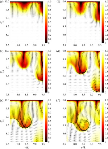
. A good correlation in the middle of the downward-falling sheets is obtained between the cold water from the surface and high scalar concentrations, which is maintained even in the head of the mushroom. As the difference in diffusivities of
$C_{\mathit{Sc}=500}$
. A good correlation in the middle of the downward-falling sheets is obtained between the cold water from the surface and high scalar concentrations, which is maintained even in the head of the mushroom. As the difference in diffusivities of $T$
and
$T$
and $C$
becomes less, areas of low
$C$
becomes less, areas of low $T$
and high
$T$
and high $C$
will tend to coincide more and more. This is illustrated in figure 12 by the almost perfect negative correlation between
$C$
will tend to coincide more and more. This is illustrated in figure 12 by the almost perfect negative correlation between $T$
and
$T$
and $C_{\mathit{Sc}=20}$
of
$C_{\mathit{Sc}=20}$
of ${\it\rho}(T,C_{\mathit{Sc}=20})\approx -0.92$
compared to values of
${\it\rho}(T,C_{\mathit{Sc}=20})\approx -0.92$
compared to values of ${\it\rho}(T,C_{\mathit{Sc}=500})$
between
${\it\rho}(T,C_{\mathit{Sc}=500})$
between $-0.455$
and
$-0.455$
and $-0.495$
.
$-0.495$
.
Simulation BC3. Correlation between temperature field and the $\mathit{Sc}=500$
scalar; the arrows illustrate the
$\mathit{Sc}=500$
scalar; the arrows illustrate the $(v,w)$
velocity field in the planes extracted at
$(v,w)$
velocity field in the planes extracted at $x/L=5$
. The isolines of
$x/L=5$
. The isolines of $C_{\mathit{Sc}=500}$
range from
$C_{\mathit{Sc}=500}$
range from $C=0.1$
to
$C=0.1$
to $0.6$
. (a)
$0.6$
. (a) $t=33.2$
s, (b)
$t=33.2$
s, (b) $t=35.1$
s, (c)
$t=35.1$
s, (c) $t=37.0$
s, (d)
$t=37.0$
s, (d) $t=38.9$
s, (e)
$t=38.9$
s, (e) $t=40.9$
s, (f)
$t=40.9$
s, (f) $t=42.8$
s.
$t=42.8$
s.
Simulation BC3. variation of the correlation of temperature and scalar concentration in time. (a) $\mathit{Sc}=20$
, (b)
$\mathit{Sc}=20$
, (b) $\mathit{Sc}=500$
.
$\mathit{Sc}=500$
.

It is interesting to study the evolution of the scalar distribution of $C_{\mathit{Sc}=500}$
in more detail. In an idealized situation, at the location where two equally strong convection cells meet, we would expect the formation of a symmetric 2D sheet of falling saturated water to form in the middle of the planar jet (corresponding to the coldest water). Because of the free-slip boundary conditions, the near-surface flow will be almost uniform. Hence, it is likely that, at the locations where convection cells meet, the relative scaling of the thermal and concentration boundary layer thicknesses (see figure 11) would be at least partially conserved in the falling sheets of cold water. Indeed, a relative scaling of
$C_{\mathit{Sc}=500}$
in more detail. In an idealized situation, at the location where two equally strong convection cells meet, we would expect the formation of a symmetric 2D sheet of falling saturated water to form in the middle of the planar jet (corresponding to the coldest water). Because of the free-slip boundary conditions, the near-surface flow will be almost uniform. Hence, it is likely that, at the locations where convection cells meet, the relative scaling of the thermal and concentration boundary layer thicknesses (see figure 11) would be at least partially conserved in the falling sheets of cold water. Indeed, a relative scaling of ${\it\delta}_{C}/{\it\delta}_{T}\approx (\mathit{Sc}/\mathit{Pr})^{-0.5}$
was retrieved in the centre of the falling sheets, where
${\it\delta}_{C}/{\it\delta}_{T}\approx (\mathit{Sc}/\mathit{Pr})^{-0.5}$
was retrieved in the centre of the falling sheets, where ${\it\delta}_{T}$
and
${\it\delta}_{T}$
and ${\it\delta}_{C}$
are the thicknesses of the thermal and concentration layers inside the sheets. This almost perfect conservation of the relative boundary layer thicknesses in the falling sheets implies that the almost uniform flow extends further down than just the near-surface region.
${\it\delta}_{C}$
are the thicknesses of the thermal and concentration layers inside the sheets. This almost perfect conservation of the relative boundary layer thicknesses in the falling sheets implies that the almost uniform flow extends further down than just the near-surface region.
4.3. Thermal boundary layer, Nusselt and Rayleigh numbers
Before the instability sets in, the colder temperature at the surface drives molecular diffusion and the thermal boundary layer thickness increases with time according to ${\it\delta}=({\rm\pi}{\it\kappa}t)^{1/2}$
, where
${\it\delta}=({\rm\pi}{\it\kappa}t)^{1/2}$
, where ${\it\kappa}$
is the thermal diffusivity (see e.g. Turner Reference Turner1979). Figure 13(a) shows the temporal variation of the thermal boundary layer thicknesses
${\it\kappa}$
is the thermal diffusivity (see e.g. Turner Reference Turner1979). Figure 13(a) shows the temporal variation of the thermal boundary layer thicknesses ${\it\delta}_{cf}$
and
${\it\delta}_{cf}$
and ${\it\delta}_{q}$
. The former is identified by the distance from the surface where the temperature fluctuation is maximum, while the latter is defined by
${\it\delta}_{q}$
. The former is identified by the distance from the surface where the temperature fluctuation is maximum, while the latter is defined by
 $$\begin{eqnarray}{\it\delta}_{q}=\frac{{\rm\Delta}T}{\left.\left(\partial T/\partial z\right)\right|_{i}},\end{eqnarray}$$
where subscript $i$
denotes the interface.
$i$
denotes the interface.
(a) Time history of thermal boundary layer thicknesses ( ${\it\delta}_{cf}$
and
${\it\delta}_{cf}$
and ${\it\delta}_{q}$
) and the resulting
${\it\delta}_{q}$
) and the resulting $\mathit{Ra}_{{\it\delta}}$
from BC3. (b) A detailed plot of the
$\mathit{Ra}_{{\it\delta}}$
from BC3. (b) A detailed plot of the ${\it\delta}_{q}$
evolution for BC3 and BC5. (c) Decrease of the temperature difference between the bulk and the surface and the corresponding
${\it\delta}_{q}$
evolution for BC3 and BC5. (c) Decrease of the temperature difference between the bulk and the surface and the corresponding $\mathit{Ra}_{L}$
with time.
$\mathit{Ra}_{L}$
with time.

The small disturbances added to the temperature field at $t=9.6~\text{s}$
were found to result in an almost instantaneous growth of the Rayleigh instability. This is proven by the fact that, immediately after the addition of the disturbances, organized fluid movements (although very small) at the top surface started to appear. Figure 13(a,b) illustrates that, at least up to
$t=9.6~\text{s}$
were found to result in an almost instantaneous growth of the Rayleigh instability. This is proven by the fact that, immediately after the addition of the disturbances, organized fluid movements (although very small) at the top surface started to appear. Figure 13(a,b) illustrates that, at least up to $t=27~\text{s}$
, diffusion dominates as the growth of the boundary layer thickness adheres to
$t=27~\text{s}$
, diffusion dominates as the growth of the boundary layer thickness adheres to ${\it\delta}=({\rm\pi}{\it\kappa}t)^{1/2}$
. At approximately
${\it\delta}=({\rm\pi}{\it\kappa}t)^{1/2}$
. At approximately $t=29.3~\text{s}$
the horizontally averaged boundary layer thickness reaches its maximum before starting to decrease abruptly. This instance matches the time when the cold fluid collected along the border of small cells first starts to plunge down in the form of thin vertical sheets and plumes. As in Howard (Reference Howard1964), the thermal boundary layer Rayleigh number
$t=29.3~\text{s}$
the horizontally averaged boundary layer thickness reaches its maximum before starting to decrease abruptly. This instance matches the time when the cold fluid collected along the border of small cells first starts to plunge down in the form of thin vertical sheets and plumes. As in Howard (Reference Howard1964), the thermal boundary layer Rayleigh number $\mathit{Ra}_{{\it\delta}}$
is defined by
$\mathit{Ra}_{{\it\delta}}$
is defined by
 $$\begin{eqnarray}\mathit{Ra}_{{\it\delta}}=\frac{{\it\alpha}{\rm\Delta}Tg{\it\delta}_{q}^{3}}{{\it\kappa}{\it\nu}}.\end{eqnarray}$$
Figure 13(b) shows a detailed plot of the thermal boundary layer evolution without and with disturbances for two different expansion factors, ${\it\alpha}{\rm\Delta}T=0.000572$
and
${\it\alpha}{\rm\Delta}T=0.000572$
and $0.000381$
, as used in BC3 and BC5, respectively. Based on the boundary layer thickness reached at the time when fluid elements first break away from the boundary layer in BC3 and BC5, critical
$0.000381$
, as used in BC3 and BC5, respectively. Based on the boundary layer thickness reached at the time when fluid elements first break away from the boundary layer in BC3 and BC5, critical $\mathit{Ra}_{{\it\delta}}$
values of approximately
$\mathit{Ra}_{{\it\delta}}$
values of approximately $2000$
and
$2000$
and $1800$
were found, respectively. The initial evolution of the thermal boundary layer thickness in all simulations with identical
$1800$
were found, respectively. The initial evolution of the thermal boundary layer thickness in all simulations with identical ${\it\alpha}{\rm\Delta}T$
and initial disturbance level was found to be the same. It should be noted that in our case
${\it\alpha}{\rm\Delta}T$
and initial disturbance level was found to be the same. It should be noted that in our case ${\rm\Delta}T$
is the temperature difference between the water surface and the bulk, while in Howard (Reference Howard1964)
${\rm\Delta}T$
is the temperature difference between the water surface and the bulk, while in Howard (Reference Howard1964) ${\rm\Delta}T$
is the temperature difference between the lower hot and upper cold surfaces. For the case of two rigid boundaries, Howard (Reference Howard1964) estimated a critical
${\rm\Delta}T$
is the temperature difference between the lower hot and upper cold surfaces. For the case of two rigid boundaries, Howard (Reference Howard1964) estimated a critical $\mathit{Ra}_{{\it\delta}}$
of the order of
$\mathit{Ra}_{{\it\delta}}$
of the order of $1000$
.
$1000$
.
In figure 13(a,b) it can also be seen that for BC3 immediately after $t=29.3~\text{s}$
both the mean boundary layer thickness and
$t=29.3~\text{s}$
both the mean boundary layer thickness and $\mathit{Ra}_{{\it\delta}}$
rapidly decrease and finally reach plateaus at approximately
$\mathit{Ra}_{{\it\delta}}$
rapidly decrease and finally reach plateaus at approximately $0.083L$
and
$0.083L$
and $18$
, respectively.
$18$
, respectively.
Figure 13(c) shows the temporal variation of ${\rm\Delta}T=\langle T_{b}\rangle -T_{s}$
, where
${\rm\Delta}T=\langle T_{b}\rangle -T_{s}$
, where $\langle \cdot \rangle$
denotes horizontal averaging, and the macroscale Rayleigh number
$\langle \cdot \rangle$
denotes horizontal averaging, and the macroscale Rayleigh number $\mathit{Ra}_{L}$
. The initial development of the instability and its affect on gas transfer across the air–water interface gives rise to time-dependent Rayleigh numbers and a time-dependent Nusselt number given by
$\mathit{Ra}_{L}$
. The initial development of the instability and its affect on gas transfer across the air–water interface gives rise to time-dependent Rayleigh numbers and a time-dependent Nusselt number given by
 $$\begin{eqnarray}\mathit{Nu}=\frac{H_{L}L}{{\it\kappa}},\end{eqnarray}$$
where $H_{L}=q/{\rm\Delta}T$
is the heat transfer coefficient and the dimensional heat flux
$H_{L}=q/{\rm\Delta}T$
is the heat transfer coefficient and the dimensional heat flux $q$
is defined by
$q$
is defined by
 $$\begin{eqnarray}q={\it\kappa}_{c}\left.\!\frac{\partial \langle T\rangle }{\partial z}\right|_{i}\frac{(T_{s}-T_{b,0})}{L},\end{eqnarray}$$
where ${\it\kappa}_{c}$
is the thermal conductivity. From the definitions above it follows that
${\it\kappa}_{c}$
is the thermal conductivity. From the definitions above it follows that
 $$\begin{eqnarray}\mathit{Nu}=(\mathit{Ra}_{L}/\mathit{Ra}_{{\it\delta}})^{1/3}\end{eqnarray}$$
(e.g. Howard Reference Howard1964). Figure 14 shows the relation between $\mathit{Nu}$
and
$\mathit{Nu}$
and $\mathit{Ra}_{{\it\delta}}$
. The data points are calculated using instantaneous horizontally averaged data. As the boundary layer thickness is correlated directly to the interfacial heat flux, the relation
$\mathit{Ra}_{{\it\delta}}$
. The data points are calculated using instantaneous horizontally averaged data. As the boundary layer thickness is correlated directly to the interfacial heat flux, the relation $\mathit{Nu}\propto \mathit{Ra}_{{\it\delta}}^{-1/3}$
holds for all times, including the diffusion-dominated regime at the beginning of the simulation and the regime where the effects of the limited depth become important at the end of the simulation. In the free-fall regime, after
$\mathit{Nu}\propto \mathit{Ra}_{{\it\delta}}^{-1/3}$
holds for all times, including the diffusion-dominated regime at the beginning of the simulation and the regime where the effects of the limited depth become important at the end of the simulation. In the free-fall regime, after $t\approx 41.3~\text{s}$
,
$t\approx 41.3~\text{s}$
, $\mathit{Ra}_{{\it\delta}}$
becomes virtually constant so that
$\mathit{Ra}_{{\it\delta}}$
becomes virtually constant so that
 $$\begin{eqnarray}\mathit{Nu}=c_{\mathit{Ra}}\mathit{Ra}_{L}^{1/3},\end{eqnarray}$$
with a value of $c_{\mathit{Ra}}$
in the region between
$c_{\mathit{Ra}}$
in the region between $0.35$
and
$0.35$
and $0.4$
(see figure 15
a). Some time after the free-fall regime, additional advective motions begin to affect the surface heat flux, resulting in a reduction in
$0.4$
(see figure 15
a). Some time after the free-fall regime, additional advective motions begin to affect the surface heat flux, resulting in a reduction in $c_{\mathit{Ra}}$
.
$c_{\mathit{Ra}}$
.
Nusselt number ( $\mathit{Nu}$
) versus boundary layer Rayleigh number (
$\mathit{Nu}$
) versus boundary layer Rayleigh number ( $\mathit{Ra}_{{\it\delta}}$
).
$\mathit{Ra}_{{\it\delta}}$
).

(a) Sensitivity of $c_{\mathit{Ra}}$
in
$c_{\mathit{Ra}}$
in $\mathit{Nu}=c_{\mathit{Ra}}\mathit{Ra}_{L}^{1/3}$
upon the selection of
$\mathit{Nu}=c_{\mathit{Ra}}\mathit{Ra}_{L}^{1/3}$
upon the selection of $z_{b}$
, which is the distance from the surface where
$z_{b}$
, which is the distance from the surface where $T_{b}$
is evaluated. (b) Evolution of the horizontally averaged temperature profile. (c) Plot of
$T_{b}$
is evaluated. (b) Evolution of the horizontally averaged temperature profile. (c) Plot of $\mathit{Nu}$
versus
$\mathit{Nu}$
versus $\mathit{Ra}_{L}$
(time averaged over
$\mathit{Ra}_{L}$
(time averaged over $t=41.3~\text{s}$
to
$t=41.3~\text{s}$
to $t=87~\text{s}$
).
$t=87~\text{s}$
).

Because the process is unsteady, the constant of proportionality $c_{\mathit{Ra}}$
in (4.7) was found to be sensitive to the distance from the surface,
$c_{\mathit{Ra}}$
in (4.7) was found to be sensitive to the distance from the surface, $z_{b}$
, where
$z_{b}$
, where $T_{b}$
was evaluated (figure 15
a,b for the case BC3). In the simulations with a domain depth
$T_{b}$
was evaluated (figure 15
a,b for the case BC3). In the simulations with a domain depth $d=10L$
(BC2 and BC3), for instance,
$d=10L$
(BC2 and BC3), for instance, $c_{\mathit{Ra}}$
slightly increased by
$c_{\mathit{Ra}}$
slightly increased by ${\approx}0.02$
when
${\approx}0.02$
when $z_{b}$
was decreased from
$z_{b}$
was decreased from $5L$
to
$5L$
to $2.5L$
. To allow a consistent comparison between simulations with different depths (figure 15
c), for this case it was decided to fix
$2.5L$
. To allow a consistent comparison between simulations with different depths (figure 15
c), for this case it was decided to fix $z_{b}$
to a value of
$z_{b}$
to a value of $2.5L$
, resulting in a constant of proportionality of
$2.5L$
, resulting in a constant of proportionality of $c_{\mathit{Ra}}=0.39$
. In the present simulations, temperature was only fixed at the top. To compare the present
$c_{\mathit{Ra}}=0.39$
. In the present simulations, temperature was only fixed at the top. To compare the present $c_{\mathit{Ra}}$
to the free-slip results of Herring (Reference Herring1963), who used fixed temperatures at top and bottom, the different definitions of
$c_{\mathit{Ra}}$
to the free-slip results of Herring (Reference Herring1963), who used fixed temperatures at top and bottom, the different definitions of ${\rm\Delta}T$
need to be taken into account. As Herring’s
${\rm\Delta}T$
need to be taken into account. As Herring’s ${\rm\Delta}T$
is twice as large, his
${\rm\Delta}T$
is twice as large, his $c_{\mathit{Ra}}$
needs to be pre-multiplied by
$c_{\mathit{Ra}}$
needs to be pre-multiplied by $2^{1/3}$
, giving a value of
$2^{1/3}$
, giving a value of ${\approx}0.39$
, which is identical to the value obtained here.
${\approx}0.39$
, which is identical to the value obtained here.
4.4. Vertical profiles
Figure 16 shows horizontally and time-averaged near-surface profiles of (a) the temperature $T$
and (b) the temperature fluctuation
$T$
and (b) the temperature fluctuation $T^{\prime }$
for various
$T^{\prime }$
for various $9.6$
s time intervals between
$9.6$
s time intervals between $t=41.3$
and
$t=41.3$
and $87~\text{s}$
. Note that the purpose of the time averaging over these short intervals is to slightly improve the statistics. When plotted against
$87~\text{s}$
. Note that the purpose of the time averaging over these short intervals is to slightly improve the statistics. When plotted against $z_{s}/{\it\delta}_{cf}$
, both the normalized mean temperature
$z_{s}/{\it\delta}_{cf}$
, both the normalized mean temperature $\langle T_{b}-T\rangle /\langle T_{b}-T_{s}\rangle$
and the normalized r.m.s. temperature
$\langle T_{b}-T\rangle /\langle T_{b}-T_{s}\rangle$
and the normalized r.m.s. temperature $T^{\prime }/\langle T_{b}-T_{s}\rangle$
profiles can be seen to collapse reasonably well. This illustrates that, in the quasi-steady state part of the free-fall regime, which is reached after a transient period (further detailed in § 4.5), the instantaneous horizontally averaged scalar profiles near the surface are approximately time-invariant (quasi-steady state). Furthermore, figure 16(a) shows that the horizontally averaged temperature eventually becomes quasi-depth-independent in the upper part of the bulk region.
$T^{\prime }/\langle T_{b}-T_{s}\rangle$
profiles can be seen to collapse reasonably well. This illustrates that, in the quasi-steady state part of the free-fall regime, which is reached after a transient period (further detailed in § 4.5), the instantaneous horizontally averaged scalar profiles near the surface are approximately time-invariant (quasi-steady state). Furthermore, figure 16(a) shows that the horizontally averaged temperature eventually becomes quasi-depth-independent in the upper part of the bulk region.
Simulation BC3. Normalized mean vertical profiles of (a) temperature and (b) temperature fluctuations.

Figure 17 shows the mean profiles of (a) the velocity fluctuations and (b) the scalar quantities $T$
and
$T$
and $C$
averaged over the entire free-fall period. The horizontal velocity fluctuations
$C$
averaged over the entire free-fall period. The horizontal velocity fluctuations $u^{\prime }$
and
$u^{\prime }$
and $v^{\prime }$
reach their maximum of
$v^{\prime }$
reach their maximum of $82\,\%$
of
$82\,\%$
of $w_{peak}^{\prime }$
at the surface where they affect the gas transfer to the unsaturated water flowing up from the bulk. For
$w_{peak}^{\prime }$
at the surface where they affect the gas transfer to the unsaturated water flowing up from the bulk. For $z_{s}>0.7L$
the horizontal fluctuations become almost constant. The vertical fluctuations reach their peak value at
$z_{s}>0.7L$
the horizontal fluctuations become almost constant. The vertical fluctuations reach their peak value at $z_{s}\approx 1.9L$
.
$z_{s}\approx 1.9L$
.
Simulation BC3. Mean vertical profiles averaged over the free-fall regime. (a) Velocity fluctuations: — ⋅ —, $u^{\prime }/w_{peak}^{\prime }$
; – – –,
$u^{\prime }/w_{peak}^{\prime }$
; – – –, $v^{\prime }/w_{peak}^{\prime }$
; ——,
$v^{\prime }/w_{peak}^{\prime }$
; ——, $w^{\prime }/w_{peak}^{\prime }$
. (b) Temperature and scalars: ——, temperature; – – –,
$w^{\prime }/w_{peak}^{\prime }$
. (b) Temperature and scalars: ——, temperature; – – –, $C_{\mathit{Sc}=20}$
; — ⋅ —,
$C_{\mathit{Sc}=20}$
; — ⋅ —, $C_{\mathit{Sc}=500}$
.
$C_{\mathit{Sc}=500}$
.

In figure 18(a) the normalized r.m.s. profiles of the temperature ( $\mathit{Pr}=6$
) and concentrations (
$\mathit{Pr}=6$
) and concentrations ( $\mathit{Sc}=20$
and
$\mathit{Sc}=20$
and $500$
) can be seen to agree reasonably well with a peak value of approximately
$500$
) can be seen to agree reasonably well with a peak value of approximately $0.25$
. The normalized diffusive and turbulent vertical mass fluxes shown in figure 18(b) were also found to collapse nicely. As expected, the turbulent vertical mass fluxes were observed to quickly increase with depth. Simultaneously, the diffusive mass flux reduced from its maximum value at the surface so that the sum of the two mass fluxes (in the region with quasi-steady horizontally averaged statistics) remained constant for all
$0.25$
. The normalized diffusive and turbulent vertical mass fluxes shown in figure 18(b) were also found to collapse nicely. As expected, the turbulent vertical mass fluxes were observed to quickly increase with depth. Simultaneously, the diffusive mass flux reduced from its maximum value at the surface so that the sum of the two mass fluxes (in the region with quasi-steady horizontally averaged statistics) remained constant for all $z_{s}$
in the upper bulk. At
$z_{s}$
in the upper bulk. At $z_{s}\approx 0.7{\it\delta}_{cf}$
the turbulent and diffusive mass fluxes were found to be equal, while for larger
$z_{s}\approx 0.7{\it\delta}_{cf}$
the turbulent and diffusive mass fluxes were found to be equal, while for larger $z_{s}$
the turbulent vertical mass flux dominated the total mass flux. Finally, for
$z_{s}$
the turbulent vertical mass flux dominated the total mass flux. Finally, for $z_{s}\geqslant 2{\it\delta}_{cf}$
the diffusive mass flux was found to be zero while the turbulent mass flux reached its maximum value of (
$z_{s}\geqslant 2{\it\delta}_{cf}$
the diffusive mass flux was found to be zero while the turbulent mass flux reached its maximum value of ( $D\partial \langle C\rangle /\partial z|_{i}$
) and fully dominated the total vertical mass flux. This result supports the usage of the eddy-correlation measurement technique (at the liquid side) in the bulk to determine the gas flux at the interface.
$D\partial \langle C\rangle /\partial z|_{i}$
) and fully dominated the total vertical mass flux. This result supports the usage of the eddy-correlation measurement technique (at the liquid side) in the bulk to determine the gas flux at the interface.
Simulation BC3. (a) Mean profiles of temperature and concentration fluctuations: ——, $T$
; – – –,
$T$
; – – –, $\mathit{Sc}=20$
; — ⋅ —,
$\mathit{Sc}=20$
; — ⋅ —, $\mathit{Sc}=500$
. (b) Mean profiles of diffusive fluxes (points:
$\mathit{Sc}=500$
. (b) Mean profiles of diffusive fluxes (points: $\boldsymbol{\cdot }\,$
,
$\boldsymbol{\cdot }\,$
, $T$
;
$T$
; $\times$
,
$\times$
, $\mathit{Sc}=20$
;
$\mathit{Sc}=20$
; $+$
,
$+$
, $\mathit{Sc}=500$
) and turbulent mass fluxes (lines: ——,
$\mathit{Sc}=500$
) and turbulent mass fluxes (lines: ——, $T$
; – – –,
$T$
; – – –, $\mathit{Sc}=20$
; — ⋅ —,
$\mathit{Sc}=20$
; — ⋅ —, $\mathit{Sc}=500$
) normalized with mass flux at the surface (
$\mathit{Sc}=500$
) normalized with mass flux at the surface ( $D\partial \langle C\rangle /\partial z|_{i}$
).
$D\partial \langle C\rangle /\partial z|_{i}$
).

Plots of (a) $K_{L}$
versus
$K_{L}$
versus $\mathit{Sc}$
(
$\mathit{Sc}$
( $\mathit{Pr}$
) and (b)
$\mathit{Pr}$
) and (b) ${\it\delta}_{cf}$
versus
${\it\delta}_{cf}$
versus $\mathit{Sc}$
(
$\mathit{Sc}$
( $\mathit{Pr}$
);
$\mathit{Pr}$
); $K_{L}$
and
$K_{L}$
and ${\it\delta}_{cf}$
time averaged from
${\it\delta}_{cf}$
time averaged from $t=41.3~\text{s}$
to
$t=41.3~\text{s}$
to $87~\text{s}$
.
$87~\text{s}$
.

4.5. Estimation of
$H_{L}$
and
$K_{L}$


In figure 6(b) the evolution of the temporal interfacial (dimensional) heat flux from BC3 was shown. With an initial temperature difference between the water surface and the bulk ( $T_{b,0}-T_{s}$
) of
$T_{b,0}-T_{s}$
) of $2.2~\text{K}$
, instantaneous peaks in the heat flux in excess of
$2.2~\text{K}$
, instantaneous peaks in the heat flux in excess of $1600~\text{W}~\text{m}^{-2}$
were observed. However, in time, the heat flux was found to slowly decrease (while the convection cell size increased). In BC5, where
$1600~\text{W}~\text{m}^{-2}$
were observed. However, in time, the heat flux was found to slowly decrease (while the convection cell size increased). In BC5, where $T_{b,0}-T_{s}$
was reduced to
$T_{b,0}-T_{s}$
was reduced to $1.48~\text{K}$
, the maximum instantaneous heat flux decreased to approximately
$1.48~\text{K}$
, the maximum instantaneous heat flux decreased to approximately $1000~\text{W}~\text{m}^{-2}$
. The reduction in the initial temperature difference from BC5 resulted in a thicker thermal boundary layer and hence a lower heat flux. The basic physical mechanism, however, is the same. Mainly because of the large initial temperature difference between the bulk and the water surface, in this study the heat fluxes were larger (though of similar order of magnitude) than most reported values observed in the oceans or lakes (e.g. Shay & Gregg Reference Shay and Gregg1984, Reference Shay and Gregg1986; MacIntyre, Romero & Kling Reference MacIntyre, Romero and Kling2002). It is clear that a one-to-one comparison between the heat fluxes obtained in the present simulations with the ones observed in nature is difficult. Apart from the additional uncertainties in nature, such as the presence of surface contamination that is known to reduce the interfacial mass transfer significantly, an accurate determination of the surface temperature in field and laboratory measurements is extremely difficult to achieve. In most experiments
$1000~\text{W}~\text{m}^{-2}$
. The reduction in the initial temperature difference from BC5 resulted in a thicker thermal boundary layer and hence a lower heat flux. The basic physical mechanism, however, is the same. Mainly because of the large initial temperature difference between the bulk and the water surface, in this study the heat fluxes were larger (though of similar order of magnitude) than most reported values observed in the oceans or lakes (e.g. Shay & Gregg Reference Shay and Gregg1984, Reference Shay and Gregg1986; MacIntyre, Romero & Kling Reference MacIntyre, Romero and Kling2002). It is clear that a one-to-one comparison between the heat fluxes obtained in the present simulations with the ones observed in nature is difficult. Apart from the additional uncertainties in nature, such as the presence of surface contamination that is known to reduce the interfacial mass transfer significantly, an accurate determination of the surface temperature in field and laboratory measurements is extremely difficult to achieve. In most experiments $T_{s}$
is assumed to be identical to the air temperature some distance above the water surface. In still air, however, the formation of a very thick thermal boundary layer on the air side will result in a significant reduction of the temperature difference between the water surface and the bulk in a matter of seconds. On the other hand, evaporation effects (not considered here, as the effects are confined to the surface, where we assume a constant temperature) may result in a surface temperature that is lower than the air temperature some distance above the interface. In the present simulations we were able to fully resolve the initial (transient) development of the Rayleigh instability with relatively large heat fluxes and steep gradients that occur in nature when the water surface is suddenly cooled.
$T_{s}$
is assumed to be identical to the air temperature some distance above the water surface. In still air, however, the formation of a very thick thermal boundary layer on the air side will result in a significant reduction of the temperature difference between the water surface and the bulk in a matter of seconds. On the other hand, evaporation effects (not considered here, as the effects are confined to the surface, where we assume a constant temperature) may result in a surface temperature that is lower than the air temperature some distance above the interface. In the present simulations we were able to fully resolve the initial (transient) development of the Rayleigh instability with relatively large heat fluxes and steep gradients that occur in nature when the water surface is suddenly cooled.
Figure 19 shows the horizontally and time-averaged gas transfer velocity and boundary layer thickness as a function of the Schmidt number. It can be seen that both $K_{L}$
and
$K_{L}$
and ${\it\delta}_{cf}$
perfectly scale with
${\it\delta}_{cf}$
perfectly scale with $\mathit{Sc}^{-0.5}$
. Time averaging was performed from
$\mathit{Sc}^{-0.5}$
. Time averaging was performed from $t=41.3~\text{s}$
to
$t=41.3~\text{s}$
to $t=87~\text{s}$
. For
$t=87~\text{s}$
. For $t\geqslant 87~\text{s}$
bottom effects became non-negligible, though the scaling of both
$t\geqslant 87~\text{s}$
bottom effects became non-negligible, though the scaling of both $K_{L}$
and
$K_{L}$
and ${\it\delta}_{cf}$
with
${\it\delta}_{cf}$
with $\mathit{Sc}^{-0.5}$
was found to persist. This is in agreement with the
$\mathit{Sc}^{-0.5}$
was found to persist. This is in agreement with the $K_{L}$
and
$K_{L}$
and ${\it\delta}$
scaling found in our previous DNS of grid-stirred turbulence-driven gas transfer (Herlina & Wissink Reference Herlina and Wissink2014) and is typical for cases with free-slip boundary conditions at the interface (perfectly clean water surface). Note that for contaminated surfaces the free-slip condition does not hold at the surface (see e.g. Khakpour et al.
Reference Khakpour, Shen and Yue2011).
${\it\delta}$
scaling found in our previous DNS of grid-stirred turbulence-driven gas transfer (Herlina & Wissink Reference Herlina and Wissink2014) and is typical for cases with free-slip boundary conditions at the interface (perfectly clean water surface). Note that for contaminated surfaces the free-slip condition does not hold at the surface (see e.g. Khakpour et al.
Reference Khakpour, Shen and Yue2011).
The Sherwood number, defined as
 $$\begin{eqnarray}\mathit{Sh}=\frac{K_{L}L}{D},\end{eqnarray}$$
is the non-dimensional transfer velocity and is analogous to the Nusselt number (4.4) used in heat transfer problems. Since $H_{L,\mathit{Pr}=6}=K_{L,\mathit{Sc}=6}$
and
$H_{L,\mathit{Pr}=6}=K_{L,\mathit{Sc}=6}$
and $K_{L}\propto \mathit{Sc}^{-0.5}$
, it immediately follows that
$K_{L}\propto \mathit{Sc}^{-0.5}$
, it immediately follows that
 $$\begin{eqnarray}\mathit{Sh}=\mathit{Nu}(\mathit{Sc}/\mathit{Pr})^{0.5}.\end{eqnarray}$$
Based on the time history shown in figures 6, 13(a,b) and 20, for BC3 it is now possible to identify three different regimes:
-
(1) Diffusive regime:
$0<t<29.3~\text{s}$
. This regime is dominated by diffusive growth of the thermal and concentration boundary layers (figure 13
a,b). It ends when the first thermal sheets and/or plumes separate from the boundary layer. Because the developing Rayleigh instability is still very weak, the surface fluctuations are very small (figure 20
a). -
(2) Free-fall regime:
$29.3~\text{s}<t<87~\text{s}$
. This regime follows the diffusive regime and ends when the near-surface fluid flow as well as the scalar transport become affected by the limited depth of the domain (figure 6). The free-fall regime can be further divided into: (i) a transient part (
$29.3~\text{s}<t<41.3~\text{s}$
) and (ii) a quasi-steady part (
$41.3~\text{s}<t<87~\text{s}$
). In the transient period, after the first plumes and/or sheets begin to fall, both
$u_{surf}^{\prime }$
and
$K_{L}$
rapidly increase. The value of
$K_{L}$
is largely independent of the convection cell size, which remains approximately constant (see figure 10). After
$t\approx 41.3~\text{s}$
the normalized horizontally averaged scalar profiles near the surface become approximately time-invariant, indicating a quasi-steady state (figure 16). Here, both
$u_{surf}^{\prime }$
and the cell size increase while
$K_{L}$
remains approximately constant. -
(3) Bottom-influenced regime:
$87~\text{s}<t<115~\text{s}$
. This regime begins when the secondary flow – induced by the plumes reaching the bottom of the domain – first affects the interfacial mass transfer. Here
$u_{surf}^{\prime }$
is found to become virtually constant while
$K_{L}$
decreases with increasing cell size.









An important aim of this study is to correlate surface information to the gas transfer velocity $K_{L}$
. As can be seen in figures 7 and 8, the near-surface flow in the present buoyancy-driven gas transfer simulations is fully dominated by large structures. Based on this observation, it can be concluded that the large-eddy model of Fortescue & Pearson (Reference Fortescue and Pearson1967) should be able to provide an accurate estimation of
$K_{L}$
. As can be seen in figures 7 and 8, the near-surface flow in the present buoyancy-driven gas transfer simulations is fully dominated by large structures. Based on this observation, it can be concluded that the large-eddy model of Fortescue & Pearson (Reference Fortescue and Pearson1967) should be able to provide an accurate estimation of $K_{L}$
. According to this model, the surface renewal rate
$K_{L}$
. According to this model, the surface renewal rate $r$
can be estimated using velocity (
$r$
can be estimated using velocity ( $U_{r}$
) and length (
$U_{r}$
) and length ( $L_{r}$
) scales that are typical for the larger structures in the flow, so that
$L_{r}$
) scales that are typical for the larger structures in the flow, so that $r=U_{r}/L_{r}$
. Buoyancy-driven flows exhibit a net-like structure of convection cells at the surface (see figure 8). The average diameter of these convection cells,
$r=U_{r}/L_{r}$
. Buoyancy-driven flows exhibit a net-like structure of convection cells at the surface (see figure 8). The average diameter of these convection cells, $L_{C}$
(see figure 10), estimated by (4.1), appears to be the appropriate choice for
$L_{C}$
(see figure 10), estimated by (4.1), appears to be the appropriate choice for $L_{r}$
. Near the interface the flow in the convection cells is almost horizontal so that
$L_{r}$
. Near the interface the flow in the convection cells is almost horizontal so that $U_{r}$
can be based on the velocity fluctuations
$U_{r}$
can be based on the velocity fluctuations $u_{surf}^{\prime }$
at the surface, defined by
$u_{surf}^{\prime }$
at the surface, defined by $u_{surf}^{\prime }=\sqrt{\overline{u^{\prime }}\overline{v^{\prime }}}$
(see figure 20
a). Hence, a renewal rate of
$u_{surf}^{\prime }=\sqrt{\overline{u^{\prime }}\overline{v^{\prime }}}$
(see figure 20
a). Hence, a renewal rate of $r=u_{surf}^{\prime }/L_{C}$
is obtained, and
$r=u_{surf}^{\prime }/L_{C}$
is obtained, and $K_{L}$
and
$K_{L}$
and $H_{L}$
can be predicted using
$H_{L}$
can be predicted using
 $$\begin{eqnarray}K_{L}=c_{K}\sqrt{Du_{surf}^{\prime }/L_{C}}\quad \text{and}\quad H_{L}=c_{H}\sqrt{{\it\kappa}u_{surf}^{\prime }/L_{C}},\end{eqnarray}$$
where $D$
and
$D$
and ${\it\kappa}$
are the scalar and thermal diffusivities, respectively.
${\it\kappa}$
are the scalar and thermal diffusivities, respectively.
Simulation BC3. (a) Horizontal surface velocity fluctuations. (b) Comparison of simulated $K_{L}$
and
$K_{L}$
and $H_{L}$
and the predictions from (4.10) with
$H_{L}$
and the predictions from (4.10) with $c_{HL}=c_{KL}=1.1$
(solid lines): ○,
$c_{HL}=c_{KL}=1.1$
(solid lines): ○, $\mathit{Pr}=6$
;
$\mathit{Pr}=6$
; $\times$
,
$\times$
, $\mathit{Sc}=20$
;
$\mathit{Sc}=20$
; $+$
,
$+$
, $\mathit{Sc}=500$
. (c) Comparison of simulated
$\mathit{Sc}=500$
. (c) Comparison of simulated $K_{L}$
and
$K_{L}$
and $H_{L}$
with
$H_{L}$
with $0.59\sqrt{D{\it\beta}^{\prime }}$
(solid lines).
$0.59\sqrt{D{\it\beta}^{\prime }}$
(solid lines).

In figure 20(b) the predictions given in (4.10) are plotted together with $K_{L}$
(for
$K_{L}$
(for $\mathit{Sc}=20$
and
$\mathit{Sc}=20$
and $500$
) and
$500$
) and $H_{L}$
. For
$H_{L}$
. For $t\geqslant 38.5~\text{s}$
a very good agreement between the aforementioned equations and both
$t\geqslant 38.5~\text{s}$
a very good agreement between the aforementioned equations and both $K_{L}$
and
$K_{L}$
and $H_{L}$
is obtained using a value of
$H_{L}$
is obtained using a value of $1.1$
for both
$1.1$
for both $c_{K}$
and
$c_{K}$
and $c_{H}$
. This good agreement is not only observed in the quasi-steady state part of the free-fall regime but also persists well after the plumes have reached the bottom of the domain and the unsteadiness introduced by the falling plumes starts to accumulate inside the computational domain. Only during the initial phase of the simulation, where diffusive mass transfer dominates the scaling of
$c_{H}$
. This good agreement is not only observed in the quasi-steady state part of the free-fall regime but also persists well after the plumes have reached the bottom of the domain and the unsteadiness introduced by the falling plumes starts to accumulate inside the computational domain. Only during the initial phase of the simulation, where diffusive mass transfer dominates the scaling of $K_{L}$
and
$K_{L}$
and $H_{L}$
, is (4.10) not applicable. Note that when replacing
$H_{L}$
, is (4.10) not applicable. Note that when replacing $L_{C}$
by
$L_{C}$
by $L_{CT}$
in (4.10) an approximation of
$L_{CT}$
in (4.10) an approximation of $K_{L}$
is obtained that is of equal quality for
$K_{L}$
is obtained that is of equal quality for $t\geqslant 50~\text{s}$
and slightly worse for
$t\geqslant 50~\text{s}$
and slightly worse for $t<50~\text{s}$
.
$t<50~\text{s}$
.
As proposed by McCready, Vassiliadou & Hanratty (Reference McCready, Vassiliadou and Hanratty1986), when very detailed surface information is available so that the surface divergence can be calculated, $K_{L}$
and
$K_{L}$
and $H_{L}$
can be estimated using
$H_{L}$
can be estimated using
 $$\begin{eqnarray}K_{L}\propto \sqrt{{\it\beta}^{\prime }D}\quad \text{and}\quad H_{L}\propto \sqrt{{\it\beta}^{\prime }{\it\kappa}},\end{eqnarray}$$
where ${\it\beta}^{\prime }$
is a measure of the surface divergence strength (see Turney & Banerjee Reference Turney and Banerjee2013) given by
${\it\beta}^{\prime }$
is a measure of the surface divergence strength (see Turney & Banerjee Reference Turney and Banerjee2013) given by
 $$\begin{eqnarray}{\it\beta}^{\prime }=\sqrt{\left\langle \left(\frac{\partial u}{\partial x}+\frac{\partial v}{\partial y}\right)^{2}\right\rangle }.\end{eqnarray}$$
In figure 20(c) a constant of proportionality of $c_{{\it\beta}}=0.59$
in (4.11) is shown to give very good approximations. Note that Turney & Banerjee (Reference Turney and Banerjee2013) recently found that surface divergence theory is not applicable when a portion of the near-surface motions holds small time scales. The time scales in the buoyancy-driven flow presented here, however, are sufficiently long for surface divergence theory to be applicable.
$c_{{\it\beta}}=0.59$
in (4.11) is shown to give very good approximations. Note that Turney & Banerjee (Reference Turney and Banerjee2013) recently found that surface divergence theory is not applicable when a portion of the near-surface motions holds small time scales. The time scales in the buoyancy-driven flow presented here, however, are sufficiently long for surface divergence theory to be applicable.
Figure 20(a) shows a comparison of $w_{peak}^{\prime }$
and
$w_{peak}^{\prime }$
and $u_{surf}^{\prime }$
against time. It can be seen that initially the qualitative behaviour of
$u_{surf}^{\prime }$
against time. It can be seen that initially the qualitative behaviour of $w_{peak}^{\prime }$
is very similar to that of
$w_{peak}^{\prime }$
is very similar to that of $K_{L}$
shown in figure 20(b,c). In the free-fall regime for
$K_{L}$
shown in figure 20(b,c). In the free-fall regime for $t\geqslant 48.1~\text{s}$
,
$t\geqslant 48.1~\text{s}$
, $w_{peak}^{\prime }$
begins to grow while
$w_{peak}^{\prime }$
begins to grow while $K_{L}$
reached a plateau. The reason for the very good initial agreement is that
$K_{L}$
reached a plateau. The reason for the very good initial agreement is that $w_{peak}^{\prime }$
is located near the surface so that
$w_{peak}^{\prime }$
is located near the surface so that $w_{peak}^{\prime }\approx w^{\prime }$
, which is strongly related to the r.m.s. of the surface divergence.
$w_{peak}^{\prime }\approx w^{\prime }$
, which is strongly related to the r.m.s. of the surface divergence.
By comparing figure 20(b) and (c) it can be seen that the quality of the estimation of $H_{L}$
and
$H_{L}$
and $K_{L}$
using (4.10) or (4.11) is similar for
$K_{L}$
using (4.10) or (4.11) is similar for $t\leqslant 87~\text{s}$
. For
$t\leqslant 87~\text{s}$
. For $t>87~\text{s}$
, when bottom effects start to become important, a slightly better estimation is obtained when using the surface divergence model (4.11).
$t>87~\text{s}$
, when bottom effects start to become important, a slightly better estimation is obtained when using the surface divergence model (4.11).
Figure 21(a,b) shows estimations of the transfer velocities in various simulations using (4.10) and (4.11), respectively. The plotted data are time-averaged over the quasi-steady part of the free-fall regime. Also displayed in figure 21(b) are results from experiments (McKenna & McGillis Reference McKenna and McGillis2004; Herlina & Jirka Reference Herlina and Jirka2008) and from the grid-stirred turbulence case of Herlina & Wissink (Reference Herlina and Wissink2014) where a $c_{{\it\beta}}$
value of 0.525 was found. In comparison, Magnaudet & Calmet (Reference Magnaudet and Calmet2006) obtained a
$c_{{\it\beta}}$
value of 0.525 was found. In comparison, Magnaudet & Calmet (Reference Magnaudet and Calmet2006) obtained a $c_{{\it\beta}}$
value of
$c_{{\it\beta}}$
value of $0.60$
for turbulent open channel flow, while Turney, Smith & Banerjee (Reference Turney, Smith and Banerjee2005) reported a
$0.60$
for turbulent open channel flow, while Turney, Smith & Banerjee (Reference Turney, Smith and Banerjee2005) reported a $c_{{\it\beta}}$
value of 0.5 in wind-driven gas transfer experiments (low and moderate wind speeds).
$c_{{\it\beta}}$
value of 0.5 in wind-driven gas transfer experiments (low and moderate wind speeds).
Estimations of $H_{L}$
and
$H_{L}$
and $K_{L}$
using data that were time-averaged over the quasi-steady part of the free-fall regime: (a) using (4.10), (b) using (4.11). The GS data points are from the numerical simulations by Herlina & Wissink (Reference Herlina and Wissink2014); the HJ and KG results are from experiments performed by Herlina & Jirka (Reference Herlina and Jirka2008) and McKenna & McGillis (Reference McKenna and McGillis2004), respectively.
$K_{L}$
using data that were time-averaged over the quasi-steady part of the free-fall regime: (a) using (4.10), (b) using (4.11). The GS data points are from the numerical simulations by Herlina & Wissink (Reference Herlina and Wissink2014); the HJ and KG results are from experiments performed by Herlina & Jirka (Reference Herlina and Jirka2008) and McKenna & McGillis (Reference McKenna and McGillis2004), respectively.

Coefficient of proportionality $c_{RT}$
in (4.13). Bulk flow properties evaluated at
$c_{RT}$
in (4.13). Bulk flow properties evaluated at $z_{s}=2.5L$
. The dashed line corresponds to
$z_{s}=2.5L$
. The dashed line corresponds to $c_{RT}=1.8$
.
$c_{RT}=1.8$
.

Above, we have shown that a very good time-accurate approximation of $K_{L}$
can be obtained using surface information. When no such information is available, it might be possible to use subsurface information instead, such as the vertical turbulent mass flux (see figure 18) or the velocity fluctuations combined with the integral length scale as detailed below. Analogously to the grid-stirred case of Herlina & Wissink (Reference Herlina and Wissink2014),
$K_{L}$
can be obtained using surface information. When no such information is available, it might be possible to use subsurface information instead, such as the vertical turbulent mass flux (see figure 18) or the velocity fluctuations combined with the integral length scale as detailed below. Analogously to the grid-stirred case of Herlina & Wissink (Reference Herlina and Wissink2014),
 $$\begin{eqnarray}K_{L}=c_{RT}u^{\prime }\mathit{Sc}^{-0.5}R_{T}^{-0.5}\end{eqnarray}$$
can be employed to estimate the transfer velocity, where the bulk turbulent Reynolds number is given by
 $$\begin{eqnarray}R_{T}=2L_{\infty }u^{\prime }/{\it\nu},\end{eqnarray}$$ $L_{\infty }$
is the integral length scale and
$L_{\infty }$
is the integral length scale and $u^{\prime }$
is the r.m.s. of the horizontal velocity fluctuations. Note that (4.13) is a variant of the large-eddy model of Fortescue & Pearson (Reference Fortescue and Pearson1967). To carry out a proper calculation of
$u^{\prime }$
is the r.m.s. of the horizontal velocity fluctuations. Note that (4.13) is a variant of the large-eddy model of Fortescue & Pearson (Reference Fortescue and Pearson1967). To carry out a proper calculation of $K_{L}$
using (4.13), bulk measurements need to be performed within the convective mixing layer. In the present simulations, a very low
$K_{L}$
using (4.13), bulk measurements need to be performed within the convective mixing layer. In the present simulations, a very low $R_{T}\leqslant 50$
was obtained. As illustrated in figure 22, a reasonable time accuracy was achieved using a coefficient of proportionality of
$R_{T}\leqslant 50$
was obtained. As illustrated in figure 22, a reasonable time accuracy was achieved using a coefficient of proportionality of $c_{RT}=1.8$
, which is comparable to the value of
$c_{RT}=1.8$
, which is comparable to the value of $1.6$
found in the grid-stirred case.
$1.6$
found in the grid-stirred case.
5. Conclusions
Large-scale DNS of mass transfer across a flat clean surface driven by buoyant convection have been carried out. The simulations are motivated by previous experiments performed at KIT (Jirka et al. Reference Jirka, Herlina and Niepelt2010). The aim of the DNS is to produce and analyse highly resolved data leading to a more in-depth and detailed understanding of the physical mechanisms that play a role in buoyancy-driven gas transfer across the air–water interface. DNS calculations allow a full control of all boundary conditions, including the temperature and possible contaminations of the water surface. In the experiments, however, such a detailed control or knowledge of surface boundary conditions is never achieved. For instance, in the experiments by Jirka et al. (Reference Jirka, Herlina and Niepelt2010), the exact surface temperature could not be measured. Furthermore, in still air the large difference in thermal diffusivities of air and water will result in the formation of a very thick thermal boundary layer on the air side of the interface. As a result, the initial temperature difference between the water surface and the bulk will significantly reduce in a matter of seconds. Evaporation, on the contrary, could result in an interfacial temperature that is lower than the air temperature above. Another problem faced by experimentalists is unwanted surface contamination that tends to inhibit the free movement of water particles along the water surface. The latter also reduces the vertical fluxes that drive the gas transfer across the air–water interface.
The simulations were performed using a code especially developed to perform highly accurate simulations of mass transfer at realistic (high) Schmidt and Prandtl numbers on a computationally feasible mesh while avoiding spurious oscillations of the scalar quantities (Kubrak et al.
Reference Kubrak, Herlina, Greve and Wissink2013). The purpose of the simulations was to investigate buoyancy-driven gas transfer across the air–water interface. The presented results are all transient and range from the onset of the Rayleigh instability until the limited depth of the domain begins to affect the gas flux at the surface. The Rayleigh instability was triggered by adding random disturbances to the temperature field at $t=9.6~\text{s}$
. The overall effect of the developing instability was found to be largely the same. In those cases where exactly the same disturbance field was employed (BC1 and BC2), it was possible to perform a one-to-one comparison of instantaneous flow, temperature and concentration fields. These fields were found to be identical until the plumes in the shallower simulation, BC1, reached the bottom of the computational domain at
$t=9.6~\text{s}$
. The overall effect of the developing instability was found to be largely the same. In those cases where exactly the same disturbance field was employed (BC1 and BC2), it was possible to perform a one-to-one comparison of instantaneous flow, temperature and concentration fields. These fields were found to be identical until the plumes in the shallower simulation, BC1, reached the bottom of the computational domain at $t\approx 48.1~\text{s}$
, while it took a further time lag of
$t\approx 48.1~\text{s}$
, while it took a further time lag of ${\rm\Delta}t=15.4~\text{s}$
before the surface heat flux was affected. Hence, to describe this evolving Rayleigh instability, depth-independent Rayleigh numbers were used, based on either the thermal boundary layer thickness or a fixed length scale
${\rm\Delta}t=15.4~\text{s}$
before the surface heat flux was affected. Hence, to describe this evolving Rayleigh instability, depth-independent Rayleigh numbers were used, based on either the thermal boundary layer thickness or a fixed length scale $L$
. For larger temperature differences between the surface and the bulk (corresponding to larger Rayleigh numbers), a faster-growing instability was obtained. Initially the thermal boundary layer thickness was fully determined by thermal diffusion. Eventually, the growing Rayleigh instability resulted in the vertical convective flux becoming strong enough to stop a further increase of the thermal boundary layer thickness. The critical boundary layer Rayleigh number,
$L$
. For larger temperature differences between the surface and the bulk (corresponding to larger Rayleigh numbers), a faster-growing instability was obtained. Initially the thermal boundary layer thickness was fully determined by thermal diffusion. Eventually, the growing Rayleigh instability resulted in the vertical convective flux becoming strong enough to stop a further increase of the thermal boundary layer thickness. The critical boundary layer Rayleigh number, $\mathit{Ra}_{{\it\delta}}$
, at maximum boundary layer thickness was found to be
$\mathit{Ra}_{{\it\delta}}$
, at maximum boundary layer thickness was found to be $\mathit{Ra}_{{\it\delta}}\approx 2000$
for the simulations with an expansion factor of
$\mathit{Ra}_{{\it\delta}}\approx 2000$
for the simulations with an expansion factor of ${\it\alpha}{\rm\Delta}T=0.572\times 10^{-3}$
and
${\it\alpha}{\rm\Delta}T=0.572\times 10^{-3}$
and $\mathit{Ra}_{{\it\delta}}\approx 1800$
for
$\mathit{Ra}_{{\it\delta}}\approx 1800$
for ${\it\alpha}{\rm\Delta}T=0.381\times 10^{-3}$
.
${\it\alpha}{\rm\Delta}T=0.381\times 10^{-3}$
.
The Rayleigh instability is seen to give rise to the formation of relatively small convection cells that tend to grow in time. At the water surface these cells are visible as a net-like structure. In the interior of the cells one or more upwellings of low-saturated warm fluid from the bulk can be found. This fluid subsequently flows radially outwards while it is cooled by the cold air and gets increasingly saturated with atmospheric gases. At the boundaries of the cells, the cooled, now heavier, fluid subsequently falls down, forming thin vertical sheets of cold fluid. In the centre plane of these sheets, where the fluid is coldest, the highest concentration of atmospheric gases was found. The scaling of the thermal boundary layer thickness ${\it\delta}_{T}=\sqrt{\mathit{Sc }/\mathit{Pr}}\,{\it\delta}_{C}$
with the concentration boundary layer thickness,
${\it\delta}_{T}=\sqrt{\mathit{Sc }/\mathit{Pr}}\,{\it\delta}_{C}$
with the concentration boundary layer thickness, ${\it\delta}_{C}$
, was found to be conserved in the sheets. The mushroom-like structures that are often reported in the literature were found to be formed at the intersection of three or more convection cells, leading to a local increase in the amount of cold fluid plunging down deep in the bulk at a relatively high velocity. Momentarily heat fluxes were obtained in excess of
${\it\delta}_{C}$
, was found to be conserved in the sheets. The mushroom-like structures that are often reported in the literature were found to be formed at the intersection of three or more convection cells, leading to a local increase in the amount of cold fluid plunging down deep in the bulk at a relatively high velocity. Momentarily heat fluxes were obtained in excess of $1600~\text{W}~\text{m}^{-2}$
. The above illustrates the effectiveness of buoyant-convective gas and heat transfer.
$1600~\text{W}~\text{m}^{-2}$
. The above illustrates the effectiveness of buoyant-convective gas and heat transfer.
The ratio of the gas transfer and the heat transfer velocities, $K_{L}/H_{L}$
, was found to be equal to
$K_{L}/H_{L}$
, was found to be equal to $(\mathit{Pr}/\mathit{Sc})^{0.5}$
. Hence, even when only information on
$(\mathit{Pr}/\mathit{Sc})^{0.5}$
. Hence, even when only information on $H_{L}$
is available, estimates of
$H_{L}$
is available, estimates of $K_{L}$
for Schmidt numbers between
$K_{L}$
for Schmidt numbers between $\mathit{Sc}=20$
up to (at least)
$\mathit{Sc}=20$
up to (at least) $\mathit{Sc}=500$
can be obtained.
$\mathit{Sc}=500$
can be obtained.
To model the renewal rate $r$
(Danckwerts Reference Danckwerts1951), it is possible to use the r.m.s. of the surface divergence
$r$
(Danckwerts Reference Danckwerts1951), it is possible to use the r.m.s. of the surface divergence ${\it\beta}^{\prime }$
as initially proposed by McCready et al. (Reference McCready, Vassiliadou and Hanratty1986). The best fit for
${\it\beta}^{\prime }$
as initially proposed by McCready et al. (Reference McCready, Vassiliadou and Hanratty1986). The best fit for $K_{L}\propto \sqrt{D{\it\beta}^{\prime }}$
was obtained using a constant of proportionality of
$K_{L}\propto \sqrt{D{\it\beta}^{\prime }}$
was obtained using a constant of proportionality of $0.59$
. Another accurate estimation of
$0.59$
. Another accurate estimation of $r$
was found using the geometric average of the r.m.s. of the velocities at the surface,
$r$
was found using the geometric average of the r.m.s. of the velocities at the surface, $u_{surf}^{\prime }=\sqrt{u^{\prime }v^{\prime }}$
, and the average size of the convection cells
$u_{surf}^{\prime }=\sqrt{u^{\prime }v^{\prime }}$
, and the average size of the convection cells $L_{C}$
, giving
$L_{C}$
, giving $K_{L}=1.1\sqrt{Du_{surf}^{\prime }/L_{C}}$
as a best fit. The average cell size
$K_{L}=1.1\sqrt{Du_{surf}^{\prime }/L_{C}}$
as a best fit. The average cell size $L_{C}$
was approximated by
$L_{C}$
was approximated by $2\sqrt{L_{x}L_{y}}$
, where
$2\sqrt{L_{x}L_{y}}$
, where $L_{x}$
and
$L_{x}$
and $L_{y}$
are the integral length scales based on
$L_{y}$
are the integral length scales based on $u$
in the
$u$
in the $x$
direction and
$x$
direction and $v$
in the
$v$
in the $y$
direction, respectively.
$y$
direction, respectively.
Above, the transfer velocity was estimated using information that is available at the water surface. The two estimations were found to have a very good time accuracy in and beyond the quasi-steady state part of the free-fall regime. When only subsurface information is available, the results showed that it is still possible to estimate $K_{L}$
with reasonable time accuracy. Such an estimation can be based, for instance, on the turbulent mass flux
$K_{L}$
with reasonable time accuracy. Such an estimation can be based, for instance, on the turbulent mass flux $\langle w^{\prime \prime }C^{\prime \prime }\rangle$
or on
$\langle w^{\prime \prime }C^{\prime \prime }\rangle$
or on $u^{\prime }$
and the integral length scale
$u^{\prime }$
and the integral length scale $L_{\infty }$
, where all quantities need to be evaluated somewhere inside the convective mixing region. The estimations will improve in time as the convective mixing layer becomes well developed.
$L_{\infty }$
, where all quantities need to be evaluated somewhere inside the convective mixing region. The estimations will improve in time as the convective mixing layer becomes well developed.
Acknowledgement
The authors would like to thank the German Research Foundation (DFG grant UH242/6-1) for funding this project, the steering committee of the Super Computing Facilities in Bavaria (HLRB) for granting computing time on SuperMUC at the Leibniz Computing Centre (LRZ) in Munich and the Steinbuch Centre for Computing (SCC) in Karlsruhe for providing computing time on the HP XC 3000. Additional funding by the Helmholtz Water Network is greatly appreciated. The anonymous referees are thanked for their constructive comments.


 Open access

