


1. Introduction
When set in motion, granular materials exhibit a range of intriguing behaviours that arise from complex interactions at the grain scale. One peculiar phenomenon is the upward curvature of the free surface of dense granular flows in certain configurations, such as open channels with frictional walls (Félix & Thomas Reference Félix and Thomas2004; Deboeuf et al. Reference Deboeuf, Lajeunesse, Dauchot and Andreotti2006; Takagi, McElwaine & Huppert Reference Takagi, McElwaine and Huppert2011; McElwaine, Takagi & Huppert Reference McElwaine, Takagi and Huppert2012), non-rectangular channel geometries (see experiments in figure 1 and § 6) and Couette cells (Dsouza & Nott Reference Dsouza and Nott2021; Cabrera & Polanía Reference Cabrera and Polanía2020). Grain-scale numerical simulations indicate that this surface deformation is accompanied by the existence of secondary counter-rotating vortices in the plane perpendicular to the main flow direction (Krishnaraj & Nott Reference Krishnaraj and Nott2016; Dsouza & Nott Reference Dsouza and Nott2021; Kim & Kamrin Reference Kim and Kamrin2023). These secondary flows have also been observed recently in experiments involving slow bulldozing of granular material using a conveyor belt (Einav et al. Reference Einav, Escobar, Baker, Guillard and Faug2024). Interestingly, both surface curvature and vortices are enhanced in flows of elongated particles, supporting the idea that these effects stem from mechanisms occurring at the grain scale (Wortel et al. Reference Wortel, Börzsönyi, Somfai, Wegner, Szabó, Stannarius and van Hecke2015; Fischer et al. Reference Fischer, Börzsönyi, Nasato, Pöschel and Stannarius2016; Mohammadi et al. Reference Mohammadi, Puzyrev, Trittel and Stannarius2022).
Dense flow of glass beads of diameter
 $d \in [125, 165] \mu$
m down an inclined channel with a parabolic cross-section in a laboratory experiment. (a–d) Snapshots of an experiment, featuring the empty channel, the propagating flow front and the steady uniform flow (see also movie 1 of the Supplementary material). The channel is coated with a rough brown sandpaper, and the laser line shows the topography. (e) Topography laser measurements for an inclination of 26
$d \in [125, 165] \mu$
m down an inclined channel with a parabolic cross-section in a laboratory experiment. (a–d) Snapshots of an experiment, featuring the empty channel, the propagating flow front and the steady uniform flow (see also movie 1 of the Supplementary material). The channel is coated with a rough brown sandpaper, and the laser line shows the topography. (e) Topography laser measurements for an inclination of 26
 $^{\circ }$
and a flux of 51 g s
$^{\circ }$
and a flux of 51 g s
 $^{-1}$
. The cross-section of the empty channel, corresponding to (a), is shown by the brown line. The surface of the steady-state granular flow, corresponding to (d), is shown by the red line and is curved upward compared with the flat black dashed line. See § 6 for additional details on the experiments.
$^{-1}$
. The cross-section of the empty channel, corresponding to (a), is shown by the brown line. The surface of the steady-state granular flow, corresponding to (d), is shown by the red line and is curved upward compared with the flat black dashed line. See § 6 for additional details on the experiments.

In dense granular flows, the surface curvature and secondary flows are generally attributed to a non-zero, negative, second-normal stress difference (between the gradient and the vorticity direction) resulting from an anisotropic distribution of the contacts at the grain scale (Nagy et al. Reference Nagy, Claudin, Börzsönyi and Somfai2020; Srivastava et al. Reference Srivastava, Silbert, Grest and Lechman2021). This is more generally related to the broken codirectionality and coaxiality between the stress and strain rate tensors, as observed in grain-scale simulations (e.g. Campbell Reference Campbell1989; Silbert et al. Reference Silbert, Ertaş, Grest, Halsey, Levine and Plimpton2001; Weinhart et al. Reference Weinhart, Hartkamp, Thornton and Luding2013; Srivastava et al. Reference Srivastava, Silbert, Grest and Lechman2021). Note, however, that both surface deformation and secondary vortices have also been reported in rapid chute flows. In that regime, they are usually attributed to fluctuations of the granular temperature, which also cause significant spatial variations in solids volume fraction (Forterre & Pouliquen Reference Forterre and Pouliquen2001; Börzsönyi et al. Reference Börzsönyi, Ecke and McElwaine2009; Brodu et al. Reference Brodu, Delannay, Valance and Richard2015).
Dense inertial granular flows are commonly described using the so-called
 $\mu (I)$
granular local rheology (GDR MiDi Reference MiDi2004; Jop, Forterre & Pouliquen Reference Jop, Forterre and Pouliquen2006). In this framework, the effective viscosity of the granular fluid depends on the local pressure due to the friction between the grains, but also on a dimensionless quantity, the inertial number
$\mu (I)$
granular local rheology (GDR MiDi Reference MiDi2004; Jop, Forterre & Pouliquen Reference Jop, Forterre and Pouliquen2006). In this framework, the effective viscosity of the granular fluid depends on the local pressure due to the friction between the grains, but also on a dimensionless quantity, the inertial number
 $I$
, which compares the time scale of macroscopic deformation with that of grain-scale rearrangements (GDR MiDi Reference MiDi2004). This constitutive law has been applied to a variety of flow configurations, including inclined channels, silo discharges and column collapses (e.g. Jop et al. Reference Jop, Forterre and Pouliquen2006; Lagrée et al. Reference Lagrée, Staron and Popinet2011; Staron, Lagrée & Popinet Reference Staron, Lagrée and Popinet2014; Martin et al. Reference Martin, Ionescu, Mangeney, Bouchut and Farin2017). However, the original
$I$
, which compares the time scale of macroscopic deformation with that of grain-scale rearrangements (GDR MiDi Reference MiDi2004). This constitutive law has been applied to a variety of flow configurations, including inclined channels, silo discharges and column collapses (e.g. Jop et al. Reference Jop, Forterre and Pouliquen2006; Lagrée et al. Reference Lagrée, Staron and Popinet2011; Staron, Lagrée & Popinet Reference Staron, Lagrée and Popinet2014; Martin et al. Reference Martin, Ionescu, Mangeney, Bouchut and Farin2017). However, the original
 $\mu (I)$
rheology has several limitations. First, it is mathematically ill-posed at both low and high values of
$\mu (I)$
rheology has several limitations. First, it is mathematically ill-posed at both low and high values of
 $I$
when combined with the canonical shape of the
$I$
when combined with the canonical shape of the
 $\mu (I)$
curve (Barker et al. Reference Barker, Schaeffer, Bohórquez and Gray2015). Partial regularisation, using a specific shape of the
$\mu (I)$
curve (Barker et al. Reference Barker, Schaeffer, Bohórquez and Gray2015). Partial regularisation, using a specific shape of the
 $\mu (I)$
curve, is then required to obtain grid-resolution convergent simulations below a critical inertial number (Barker et al. Reference Barker, Schaeffer, Shearer and Gray2017, Reference Barker, Rauter, Maguire, Johnson and Gray2021; Maguire et al. Reference Maguire, Barker, Rauter, Johnson and Gray2024; Lloyd et al. Reference Lloyd, Maguire, Mistry, Reynolds, Johnson and Gray2025). Second, the original form of this rheology cannot account for certain phenomena observed in experiments or grain-scale simulations. For instance, some flows can dilate and contract, motivating the development of compressible extensions in which the volume fraction
$\mu (I)$
curve, is then required to obtain grid-resolution convergent simulations below a critical inertial number (Barker et al. Reference Barker, Schaeffer, Shearer and Gray2017, Reference Barker, Rauter, Maguire, Johnson and Gray2021; Maguire et al. Reference Maguire, Barker, Rauter, Johnson and Gray2024; Lloyd et al. Reference Lloyd, Maguire, Mistry, Reynolds, Johnson and Gray2025). Second, the original form of this rheology cannot account for certain phenomena observed in experiments or grain-scale simulations. For instance, some flows can dilate and contract, motivating the development of compressible extensions in which the volume fraction
 $\varPhi$
also depends on the inertial number, in addition to the friction coefficient
$\varPhi$
also depends on the inertial number, in addition to the friction coefficient
 $\mu$
(GDR MiDi Reference MiDi2004; Pouliquen et al. Reference Pouliquen, Cassar, Jop, Forterre and Nicolas2006; Forterre & Pouliquen Reference Forterre and Pouliquen2008). However, such compressible
$\mu$
(GDR MiDi Reference MiDi2004; Pouliquen et al. Reference Pouliquen, Cassar, Jop, Forterre and Nicolas2006; Forterre & Pouliquen Reference Forterre and Pouliquen2008). However, such compressible
 $\mu (I)$
models are generally ill-posed unless formulated under specific frameworks (Barker et al. Reference Barker, Schaeffer, Shearer and Gray2017; Heyman et al. Reference Heyman, Delannay, Tabuteau and Valance2017; Schaeffer et al. Reference Schaeffer, Barker, Tsuji, Gremaud, Shearer and Gray2019). Moreover, some flows exhibit non-local effects responsible for the slow creeping motions observed in heap flows far from the free surface (Komatsu et al. Reference Komatsu, Inagaki, Nakagawa and Nasuno2001) or coexisting adjacent static and flowing regions (e.g. Edwards & Gray Reference Edwards and Gray2015; Rocha, Johnson & Gray Reference Rocha, Johnson and Gray2019), which lead to corresponding extensions of the
$\mu (I)$
models are generally ill-posed unless formulated under specific frameworks (Barker et al. Reference Barker, Schaeffer, Shearer and Gray2017; Heyman et al. Reference Heyman, Delannay, Tabuteau and Valance2017; Schaeffer et al. Reference Schaeffer, Barker, Tsuji, Gremaud, Shearer and Gray2019). Moreover, some flows exhibit non-local effects responsible for the slow creeping motions observed in heap flows far from the free surface (Komatsu et al. Reference Komatsu, Inagaki, Nakagawa and Nasuno2001) or coexisting adjacent static and flowing regions (e.g. Edwards & Gray Reference Edwards and Gray2015; Rocha, Johnson & Gray Reference Rocha, Johnson and Gray2019), which lead to corresponding extensions of the
 $\mu (I)$
rheology (Pouliquen & Forterre Reference Pouliquen and Forterre2009; Bouzid et al. Reference Bouzid, Izzet, Trulsson, Clément, Claudin and Andreotti2015; Kamrin Reference Kamrin2019).
$\mu (I)$
rheology (Pouliquen & Forterre Reference Pouliquen and Forterre2009; Bouzid et al. Reference Bouzid, Izzet, Trulsson, Clément, Claudin and Andreotti2015; Kamrin Reference Kamrin2019).
To account for broken codirectionality, broken coaxiality and the existence of normal stress differences, the
 $\mu (I)$
rheology can also be extended to a second-order formulation, similar to the general form of a second-order fluid, also known as the Rivlin–Ericksen fluid of second grade (Rivlin & Ericksen Reference Rivlin and Ericksen1997; McElwaine et al. Reference McElwaine, Takagi and Huppert2012; Srivastava et al. Reference Srivastava, Silbert, Grest and Lechman2021). Recently, this second-order rheology has also been extended to incorporate non-locality (Kim & Kamrin Reference Kim and Kamrin2023). Using the local version of this second-order rheology, McElwaine et al. (Reference McElwaine, Takagi and Huppert2012) linked the upward surface curvature to the cross-stream gradient of the streamwise velocity, induced by friction on static levees present on the sides. However, the lack of a closure describing the flow behaviour at the interface between flowing and static regions prevented a complete resolution of the problem. Recently, Kim & Kamrin (Reference Kim and Kamrin2023) numerically solved the continuum mass and momentum equations using this second-order rheology and successfully reproduced the secondary flows observed in fully discrete, grain-scale simulations, in which the momentum balance is solved for each particle using the discrete element method (DEM). However, rather than solving the complete free-boundary problem, they imposed spatial boundary conditions (including the free surface shape) directly extracted from the DEM simulations. Hence, a complete model of the entire flow structure in open channels remains elusive.
$\mu (I)$
rheology can also be extended to a second-order formulation, similar to the general form of a second-order fluid, also known as the Rivlin–Ericksen fluid of second grade (Rivlin & Ericksen Reference Rivlin and Ericksen1997; McElwaine et al. Reference McElwaine, Takagi and Huppert2012; Srivastava et al. Reference Srivastava, Silbert, Grest and Lechman2021). Recently, this second-order rheology has also been extended to incorporate non-locality (Kim & Kamrin Reference Kim and Kamrin2023). Using the local version of this second-order rheology, McElwaine et al. (Reference McElwaine, Takagi and Huppert2012) linked the upward surface curvature to the cross-stream gradient of the streamwise velocity, induced by friction on static levees present on the sides. However, the lack of a closure describing the flow behaviour at the interface between flowing and static regions prevented a complete resolution of the problem. Recently, Kim & Kamrin (Reference Kim and Kamrin2023) numerically solved the continuum mass and momentum equations using this second-order rheology and successfully reproduced the secondary flows observed in fully discrete, grain-scale simulations, in which the momentum balance is solved for each particle using the discrete element method (DEM). However, rather than solving the complete free-boundary problem, they imposed spatial boundary conditions (including the free surface shape) directly extracted from the DEM simulations. Hence, a complete model of the entire flow structure in open channels remains elusive.
Surface deformation and secondary flows are also observed in other types of non-Newtonian fluids, such as viscoelastic fluids or dense suspensions (e.g. Maklad & Poole Reference Maklad and Poole2021). Dense suspensions, in particular, share several features with dense granular flows due to the frictional interactions between the particles forming the suspension (Guazzelli & Pouliquen Reference Guazzelli and Pouliquen2018). In their case, the second-normal stress difference has been measured using standard rheometer geometries (Singh & Nott Reference Singh and Nott2003; Dbouk, Lobry & Lemaire Reference Dbouk, Lobry and Lemaire2013), but also using an alternative approach based on the measurement of the surface deformation in Weissenberg (rotating-rod) and tilted-trough geometries, in which confinement effects can be reduced and sensitivity improved (Boyer, Pouliquen & Guazzelli Reference Boyer, Pouliquen and Guazzelli2011; Couturier et al. Reference Couturier, Boyer, Pouliquen and Guazzelli2011; Dai et al. Reference Dai, Bertevas, Qi and Tanner2013). However, these approaches rely on a known relation between the normal stress difference and the surface deformation, which is currently lacking in the case of dense granular flows.
This paper starts by extending the approach of McElwaine et al. (Reference McElwaine, Takagi and Huppert2012) by considering a steady granular flow inside a tilted channel of general (but smooth) cross-section, and derives asymptotic solutions for the flow structure and surface deformation. These solutions are then compared with the results of DEM simulations, which they match quantitatively. Finally, laboratory experiments are performed, in which simple measurements of the surface deformation and the channel shape are used to infer measurements of the second-normal stress differences using the results of the mathematical model.
2. Governing equations and second-order granular rheology
2.1. System and governing equations
The system considered here is sketched in figure 2. It consists of a dense flow of particles, of diameter
 $d$
and intrinsic density
$d$
and intrinsic density
 $\rho_{\textit{p}}$
, down an inclined channel of arbitrary cross-section. Let
$\rho_{\textit{p}}$
, down an inclined channel of arbitrary cross-section. Let
 $\textit{Oxyz}$
be a Cartesian coordinate system with the
$\textit{Oxyz}$
be a Cartesian coordinate system with the
 $x$
-axis oriented down the slope, at an angle
$x$
-axis oriented down the slope, at an angle
 $\theta$
to the horizontal, and the
$\theta$
to the horizontal, and the
 $y$
-axis and
$y$
-axis and
 $z$
-axis oriented in the cross-slope and upward normal directions, respectively. The flow has velocity components in the three directions, i.e.
$z$
-axis oriented in the cross-slope and upward normal directions, respectively. The flow has velocity components in the three directions, i.e.
 $\boldsymbol{u} = (u, v, w)$
and a bulk density
$\boldsymbol{u} = (u, v, w)$
and a bulk density
 $\rho = \varPhi \rho_{\textit{p}}$
, where
$\rho = \varPhi \rho_{\textit{p}}$
, where
 $\varPhi$
is the solids volume fraction.
$\varPhi$
is the solids volume fraction.
Conceptual sketch corresponding to the laboratory experiment shown in figure 1 and movie 1 of the Supplementary material, showing the base shape, surface curvature and flow structure. The velocity
 $\boldsymbol{u} = (u, v, w)$
has a main component in the downslope direction
$\boldsymbol{u} = (u, v, w)$
has a main component in the downslope direction
 $x$
, and secondary flows
$x$
, and secondary flows
 $(v, w)$
in the cross-slope and normal directions. Note that the aspect ratio has been increased compared with the shallow flows considered here for the sake of clarity.
$(v, w)$
in the cross-slope and normal directions. Note that the aspect ratio has been increased compared with the shallow flows considered here for the sake of clarity.

The dynamics is then governed by the mass conservation equation,
 \begin{equation} \frac {\partial \rho }{\partial t} + {\boldsymbol{\nabla }} \boldsymbol{\cdot } \left (\rho \boldsymbol{u}\right ) = 0, \end{equation}
and the momentum balance equation,
 \begin{equation} \rho \frac {\partial \boldsymbol{u}}{\partial t} + \rho (\boldsymbol{u} \boldsymbol{\cdot } {\boldsymbol{\nabla }})\boldsymbol{u} = {\boldsymbol{\nabla }} \boldsymbol{\cdot } \boldsymbol{\sigma } + \rho \boldsymbol{g}, \end{equation}
where
 $\boldsymbol{\nabla }$
is the gradient operator, ‘
$\boldsymbol{\nabla }$
is the gradient operator, ‘
 $\boldsymbol{\cdot }$
’ the dot product,
$\boldsymbol{\cdot }$
’ the dot product,
 $\boldsymbol{\sigma }$
the Cauchy stress tensor and
$\boldsymbol{\sigma }$
the Cauchy stress tensor and
 $\boldsymbol{g} = g(\sin \theta , 0, -\cos \theta )$
the gravitational acceleration.
$\boldsymbol{g} = g(\sin \theta , 0, -\cos \theta )$
the gravitational acceleration.
2.2. The second-order granular rheology
To the authors’ knowledge, the only granular constitutive model to include the non-coaxiality and non-codirectionality between principal directions of stress and strain rate tensors, and therefore also accounting for both the first- and second-normal stress differences, is constructed as a series of Rivlin–Ericksen tensors (Rivlin & Ericksen Reference Rivlin and Ericksen1997; McElwaine et al. Reference McElwaine, Takagi and Huppert2012; Wu et al. Reference Wu, Aubry, Antaki and Massoudi2017; Srivastava et al. Reference Srivastava, Silbert, Grest and Lechman2021; Kim & Kamrin Reference Kim and Kamrin2023). Note that this rheology neglects any elastic effects and assumes that non-hydrostatic stresses emerge only from the flow and are then zero when the material is at rest (Srivastava et al. Reference Srivastava, Silbert, Grest and Lechman2021). The strain rate and spin rate tensors,
 $\unicode{x1D63F}$
and
$\unicode{x1D63F}$
and
 $\unicode{x1D652}$
, are defined from the velocity gradient
$\unicode{x1D652}$
, are defined from the velocity gradient
 ${\boldsymbol{\nabla \!}}\boldsymbol{u}$
as
${\boldsymbol{\nabla \!}}\boldsymbol{u}$
as
 \begin{equation} \unicode{x1D63F} = \dfrac {1}{2} ({\boldsymbol{\nabla \!}}\boldsymbol{u} + {\boldsymbol{\nabla \!}}\boldsymbol{u}^{T} ), \qquad \unicode{x1D652} = \dfrac {1}{2} ({\boldsymbol{\nabla \!}}\boldsymbol{u} - {\boldsymbol{\nabla \!}}\boldsymbol{u}^{T} ). \end{equation}
The second-order Cauchy stress tensor is then
 \begin{equation} \begin{aligned} \boldsymbol{\sigma } = \, & p \left (\!-\unicode{x1D644} + \frac {\mu _{1}}{\left \lVert \unicode{x1D63F}\right \rVert }\left [\unicode{x1D63F} - \frac {1}{3}\text {tr}(\unicode{x1D63F}\kern1pt )\unicode{x1D644} \right ] - \frac {\mu _{2}}{\left \lVert \unicode{x1D63F}\right \rVert ^{2}}\!\left [\unicode{x1D63F}^{{\kern1pt}2} - \frac {1}{3}\text {tr} (\unicode{x1D63F}^{{\kern1pt}2})\unicode{x1D644} \right ] - \frac {\mu _{3}}{\left \lVert \unicode{x1D63F}\right \rVert ^{2}} \kern2pt \mathring {\kern-2pt \unicode{x1D63F}}\right )\!, \end{aligned} \end{equation}
where
 $p \equiv -\text {tr} (\boldsymbol{\sigma } )/3$
is the pressure, since all but the unit tensor
$p \equiv -\text {tr} (\boldsymbol{\sigma } )/3$
is the pressure, since all but the unit tensor
 $\unicode{x1D644}$
are deviatoric,
$\unicode{x1D644}$
are deviatoric,
 $\left \lVert \unicode{x1D63F}\right \rVert$
is the second invariant of the strain-rate tensor,
$\left \lVert \unicode{x1D63F}\right \rVert$
is the second invariant of the strain-rate tensor,
 \begin{equation} \left \lVert \unicode{x1D63F}\right \rVert = \sqrt {\frac {1}{2}\text {tr} (\unicode{x1D63F}^{{\kern1pt}2})}, \end{equation}
and
 $\kern2pt \mathring { \kern-2pt D}$
is the Jaumann derivative,
$\kern2pt \mathring { \kern-2pt D}$
is the Jaumann derivative,
 \begin{equation} \kern2pt \mathring {\kern-2pt \unicode{x1D63F}} = \dot {\unicode{x1D63F}} - \unicode{x1D652}\unicode{x1D63F} + \unicode{x1D63F}\unicode{x1D652}, \end{equation}
where
 $\dot {\unicode{x1D63F}} = \partial \unicode{x1D63F}/ \partial t + (\boldsymbol{u} \boldsymbol{\cdot } {\boldsymbol{\nabla }} )\unicode{x1D63F}$
is the material derivative. In principle, the rheological coefficients
$\dot {\unicode{x1D63F}} = \partial \unicode{x1D63F}/ \partial t + (\boldsymbol{u} \boldsymbol{\cdot } {\boldsymbol{\nabla }} )\unicode{x1D63F}$
is the material derivative. In principle, the rheological coefficients
 $\mu _{1}$
,
$\mu _{1}$
,
 $\mu _{2}$
and
$\mu _{2}$
and
 $\mu _{3}$
may depend on any dimensionless parameters of the system, such as the volume fraction, the dimensionless granular temperature (Kim & Kamrin Reference Kim and Kamrin2020, Reference Kim and Kamrin2023), or the inertial number,
$\mu _{3}$
may depend on any dimensionless parameters of the system, such as the volume fraction, the dimensionless granular temperature (Kim & Kamrin Reference Kim and Kamrin2020, Reference Kim and Kamrin2023), or the inertial number,
 \begin{equation} I = \dfrac {\dot {\gamma } d}{\sqrt {p/\rho _{p}}}, \end{equation}
corresponding to a ratio of time scales at the particle scale,
 $d/\sqrt {p/\rho_{\textit{p}}}$
, and at the flow scale,
$d/\sqrt {p/\rho_{\textit{p}}}$
, and at the flow scale,
 $1/\dot {\gamma }$
. Here, the definition of the shear rate is
$1/\dot {\gamma }$
. Here, the definition of the shear rate is
 \begin{equation} \dot {\gamma } = 2\left \lVert \unicode{x1D63F}\right \rVert \!. \end{equation}
In practice, the rheological coefficients have been shown using DEM simulations to predominantly depend on the inertial number (GDR MiDi Reference MiDi2004; Srivastava et al. Reference Srivastava, Silbert, Grest and Lechman2021). Note that this is not the case for flows very close to rest (typically
 $I \lt 10^{-2}$
), where these coefficients also depend on the granular temperature/fluidity as non-locality needs to be taken into account (Kim & Kamrin Reference Kim and Kamrin2020, Reference Kim and Kamrin2023). However, the inertial number is assumed to be large enough for these effects to be negligible.
$I \lt 10^{-2}$
), where these coefficients also depend on the granular temperature/fluidity as non-locality needs to be taken into account (Kim & Kamrin Reference Kim and Kamrin2020, Reference Kim and Kamrin2023). However, the inertial number is assumed to be large enough for these effects to be negligible.
Although various functional forms can be used to represent
 $\mu _{1}(I)$
,
$\mu _{1}(I)$
,
 $\mu _{2}(I)$
and
$\mu _{2}(I)$
and
 $\mu _{3}(I)$
, the following derivations can be made without prescribing any specific form. This is because the inertial number is constant at leading order (see § 4.1) and the first-order cross-stream and normal velocities are not coupled to the first-order corrections to the inertial number (see § 4.2). In the classical
$\mu _{3}(I)$
, the following derivations can be made without prescribing any specific form. This is because the inertial number is constant at leading order (see § 4.1) and the first-order cross-stream and normal velocities are not coupled to the first-order corrections to the inertial number (see § 4.2). In the classical
 $\mu (I)$
rheology (Jop et al. Reference Jop, Forterre and Pouliquen2006), which is recovered by neglecting the second-order terms and compressibility (
$\mu (I)$
rheology (Jop et al. Reference Jop, Forterre and Pouliquen2006), which is recovered by neglecting the second-order terms and compressibility (
 $\text {tr} (\unicode{x1D63F} \kern1pt ) = 0$
), the Cauchy stress,
$\text {tr} (\unicode{x1D63F} \kern1pt ) = 0$
), the Cauchy stress,
 \begin{equation} \boldsymbol{\sigma } = p\!\left [-\unicode{x1D644} + \mu _{1}(I)\frac {\unicode{x1D63F}}{\left \lVert \unicode{x1D63F}\right \rVert } \right ]\!, \end{equation}
and the form of
 $\mu _{1}(I)$
determines the region of
$\mu _{1}(I)$
determines the region of
 $I$
over which the rheology is well-posed (Barker et al. Reference Barker, Schaeffer, Bohórquez and Gray2015, Reference Barker, Schaeffer, Shearer and Gray2017). The form of
$I$
over which the rheology is well-posed (Barker et al. Reference Barker, Schaeffer, Bohórquez and Gray2015, Reference Barker, Schaeffer, Shearer and Gray2017). The form of
 $\mu _{2}(I)$
and
$\mu _{2}(I)$
and
 $\mu _{3}(I)$
will influence the well-posedness of the second-order rheology (3.3), but whether the resulting equations are well-posed or ill-posed is as yet unknown. Analysis of well-posedness would be essential for studying time-dependent solutions of (3.3), but this lies beyond the scope of this study, which focuses on steady-state solutions, where ill-posedness is not an issue.
$\mu _{3}(I)$
will influence the well-posedness of the second-order rheology (3.3), but whether the resulting equations are well-posed or ill-posed is as yet unknown. Analysis of well-posedness would be essential for studying time-dependent solutions of (3.3), but this lies beyond the scope of this study, which focuses on steady-state solutions, where ill-posedness is not an issue.
The loss of coaxiality between stress and strain-rate included in the constitutive model (2.4) corresponds to the existence of normal stress differences: the diagonal components of the stress are no longer equal (in contrast to the first-order
 $\mu (I)$
rheology (2.9)). These effects are usually described by the canonical first- and second-normal stress differences, which are defined relative to the local coordinate system formed by the flow: flow direction, the velocity-gradient direction and the vorticity direction. The first normal stress difference is the stress difference between the flow and gradient directions, while the second is the difference between the gradient and vorticity directions. The local flow coordinate system generally depends on space and time; only under additional kinematic assumptions (see § 4) can they be identified with the Cartesian coordinate system
$\mu (I)$
rheology (2.9)). These effects are usually described by the canonical first- and second-normal stress differences, which are defined relative to the local coordinate system formed by the flow: flow direction, the velocity-gradient direction and the vorticity direction. The first normal stress difference is the stress difference between the flow and gradient directions, while the second is the difference between the gradient and vorticity directions. The local flow coordinate system generally depends on space and time; only under additional kinematic assumptions (see § 4) can they be identified with the Cartesian coordinate system
 $\textit{Oxyz}$
.
$\textit{Oxyz}$
.
2.3. Boundary conditions
The kinematic and dynamic boundary conditions at the flow surface
 $s$
are
$s$
are
 \begin{align} \frac {\partial s}{\partial t} + \boldsymbol{n} \boldsymbol{\cdot } \boldsymbol{u} & = 0, \quad z = s, {} \end{align}
 \begin{align} \boldsymbol{\sigma } \boldsymbol{\cdot } \boldsymbol{n} & = \boldsymbol{0}, \quad z = s, \end{align}
where
 $\boldsymbol{n}$
is a unit vector normal to the flow surface. Additionally, there is no slip at the base
$\boldsymbol{n}$
is a unit vector normal to the flow surface. Additionally, there is no slip at the base
 $b$
, such that
$b$
, such that
 \begin{equation} \boldsymbol{u} = \boldsymbol{0}, \quad z = b. \end{equation}
3. Assumptions and reduced problem
3.1. Governing equations
Motivated by the experiments shown in figure 1 and movie 1 of the Supplementary material, the system is assumed to be steady in time and invariant along the
 $x$
-axis, such that the flow velocity only depends on
$x$
-axis, such that the flow velocity only depends on
 $y$
and
$y$
and
 $z$
while the flow height
$z$
while the flow height
 $h$
and channel cross-section
$h$
and channel cross-section
 $b$
only depend on
$b$
only depend on
 $y$
. The solids volume fraction
$y$
. The solids volume fraction
 $\varPhi$
and the bulk flow density (
$\varPhi$
and the bulk flow density (
 $\rho = \varPhi \rho_{\textit{p}}$
) are also assumed to be constant and uniform (GDR MiDi Reference MiDi2004). Under those assumptions, the mass and momentum equations reduce to
$\rho = \varPhi \rho_{\textit{p}}$
) are also assumed to be constant and uniform (GDR MiDi Reference MiDi2004). Under those assumptions, the mass and momentum equations reduce to
 \begin{align} {\boldsymbol{\nabla }} \boldsymbol{\cdot } \boldsymbol{u} & = 0, \\[-9pt] \nonumber \end{align}
 \begin{align} \rho (\boldsymbol{u} \boldsymbol{\cdot } {\boldsymbol{\nabla }})\boldsymbol{u} & = {\boldsymbol{\nabla }} \boldsymbol{\cdot } \boldsymbol{\sigma } + \rho \boldsymbol{g}. \end{align}
The Cauchy stress tensor also simplifies to
 \begin{equation} \boldsymbol{\sigma } = p\! \left (\!-\unicode{x1D644} + \frac {\mu _{1}}{\left \lVert \unicode{x1D63F}\right \rVert }\unicode{x1D63F} - \frac {\mu _{2}}{\left \lVert \unicode{x1D63F}\right \rVert ^{2}}\left [\unicode{x1D63F}^{{\kern1pt}2} - \frac {1}{3}\text {tr} (\unicode{x1D63F}^{{\kern1pt}2})\unicode{x1D644} \right ] - \frac {\mu _{3}}{\left \lVert \unicode{x1D63F}\right \rVert ^{2}} [ (\boldsymbol{u} \boldsymbol{\cdot } {\boldsymbol{\nabla }}) \unicode{x1D63F} - \unicode{x1D652}\unicode{x1D63F} + \unicode{x1D63F}\unicode{x1D652} \kern1pt ]\right )\!, \end{equation}
as mass conservation implies that
 $\text {tr} (\unicode{x1D63F} \kern1pt ) = 0$
.
$\text {tr} (\unicode{x1D63F} \kern1pt ) = 0$
.
3.2. Boundary conditions
Under those assumptions, the boundary conditions at the flow surface (2.10) and (2.11) reduce to
 \begin{align} v s_{y} & = w, \ \ \, \quad z = s, \end{align}
 \begin{align} \sigma ^{xy} s_{y} & = \sigma ^{xz}, \quad z = s, \end{align}
 \begin{align} \sigma ^{yy} s_{y} & = \sigma ^{yz}, \quad z = s, \end{align}
 \begin{align} \sigma ^{zy} s_{y} & = \sigma ^{zz},\kern0.75pt \quad z = s. \end{align}
The subscript notation is used for derivatives in this paper, such that
 $\partial X/\partial y = X_{y}$
for the
$\partial X/\partial y = X_{y}$
for the
 $y$
coordinate, and similarly for the
$y$
coordinate, and similarly for the
 $z$
coordinate. Additionally, the flow depth is zero at the lateral edges,
$z$
coordinate. Additionally, the flow depth is zero at the lateral edges,
 \begin{equation} s = b, \quad y = \pm \frac {W}{2}, \end{equation}
where
 $W$
is the cross-stream horizontal extent of the flow. Finally, the conservation of the mass flux,
$W$
is the cross-stream horizontal extent of the flow. Finally, the conservation of the mass flux,
 \begin{equation} Q = \rho \int _{-W/2}^{W/2} \int _{b(y)}^{s(y)} u(y, z)\, \text {d}z\, \text {d}y, \end{equation}
will be used to make comparisons between the mathematical model, the experiments and the numerical simulations.
3.3. Scalings and dimensionless equations
Neglecting the normal stress differences, properties of downslope steady-state granular flows result from a balance between friction and gravity (e.g. GDR MiDi Reference MiDi2004), such that
 \begin{equation} \mu _{1}\mathcal{P} \sim \rho g \mathcal{H} \sin \theta , \end{equation}
where
 $\mathcal{H}$
and
$\mathcal{H}$
and
 $\mathcal{P}$
are the characteristic height and pressure scales. As the pressure is hydrostatic,
$\mathcal{P}$
are the characteristic height and pressure scales. As the pressure is hydrostatic,
 \begin{equation} \mathcal{P} \sim \rho g \mathcal{H} \cos \theta , \end{equation}
this leads to
 $\mu _{1}(\mathcal{I}) \sim \tan \theta$
, or equivalently to a characteristic inertial number,
$\mu _{1}(\mathcal{I}) \sim \tan \theta$
, or equivalently to a characteristic inertial number,
 \begin{equation} \mathcal{I} = \mu _{1}^{-1}(\tan \theta ). \end{equation}
The inertial number is then controlled by the slope, but also the friction law of the considered granular media.
As the shear rate is dominated by the vertical velocity gradient
 $\mathcal{U}/\mathcal{H}$
, (2.7) implies a Bagnold scaling for the velocity
$\mathcal{U}/\mathcal{H}$
, (2.7) implies a Bagnold scaling for the velocity
 \begin{equation} \mathcal{U} \sim \mathcal{I} \frac {\mathcal{H}^{3/2}}{d}\sqrt {\varPhi g \cos \theta }. \end{equation}
The characteristic vertical and horizontal length scales,
 $\mathcal{H}$
and
$\mathcal{H}$
and
 $\mathcal{W}$
, can be determined by rewriting dimensionally the edge condition (3.8) and the flux conservation (3.9) as
$\mathcal{W}$
, can be determined by rewriting dimensionally the edge condition (3.8) and the flux conservation (3.9) as
 \begin{align} \mathcal{H} & = b\left (\frac {\mathcal{W}}{2}\right )\!, \\[-10pt] \nonumber \end{align}
 \begin{align} Q & \sim \rho \mathcal{U} \mathcal{H} \mathcal{W}, \end{align}
which form, together with (3.13), a system of three equations with three unknowns,
 $\mathcal{U}$
,
$\mathcal{U}$
,
 $\mathcal{H}$
and
$\mathcal{H}$
and
 $\mathcal{W}$
.
$\mathcal{W}$
.
The characteristic scales defined by (3.11), (3.12), (3.13), (3.14) and (3.15) can then be computed by prescribing values for
 $d$
,
$d$
,
 $\rho_{\textit{p}}$
,
$\rho_{\textit{p}}$
,
 $\varPhi$
,
$\varPhi$
,
 $g$
,
$g$
,
 $\theta$
,
$\theta$
,
 $Q$
, the base shape
$Q$
, the base shape
 $b(y)$
and a friction law
$b(y)$
and a friction law
 $\mu _{1}(I)$
. Note that, instead of a friction law, it is also possible to specify a value of
$\mu _{1}(I)$
. Note that, instead of a friction law, it is also possible to specify a value of
 $\mathcal{I}$
and compute
$\mathcal{I}$
and compute
 $\mu _{1}$
from
$\mu _{1}$
from
 $\tan \theta$
.
$\tan \theta$
.
These scales suggest introducing dimensionless variables, indicated by the tilde, as
 \begin{align} (z, s, y, W) & = \mathcal{H} \left (\tilde {z}, \tilde {s}, \frac {\tilde {y}}{\varepsilon }, \frac {\tilde {W}}{\varepsilon }\right )\!, \end{align}
 \begin{align} \boldsymbol{u} & = \mathcal{U} \tilde {\boldsymbol{u}},\\[-10pt] \nonumber \end{align}
 \begin{align} (p, \boldsymbol{\sigma }) & = \mathcal{P} (\tilde {p}, \tilde {\boldsymbol{\sigma }}), \\[-10pt] \nonumber \end{align}
 \begin{align} I & = \mathcal{I} \tilde {I}, \end{align}
where
 $\varepsilon = \mathcal{H}/\mathcal{W}$
accounts for the spanwise shallowness of the flow. Note that the inertial number
$\varepsilon = \mathcal{H}/\mathcal{W}$
accounts for the spanwise shallowness of the flow. Note that the inertial number
 $I$
, although already dimensionless, is still scaled so that all leading-order quantities are of order
$I$
, although already dimensionless, is still scaled so that all leading-order quantities are of order
 $O(1)$
. The dimensionless momentum and mass balance equations then become
$O(1)$
. The dimensionless momentum and mass balance equations then become
 \begin{align} \varepsilon \tilde {v}_{\tilde {y}} + \tilde {w}_{\tilde {z}} & = 0, \end{align}
 \begin{align} {\textit {Fr}}^{2} (\varepsilon \tilde {v} \tilde {u}_{\tilde {y}} + \tilde {w} \tilde {u}_{\tilde {z}} ) & = \tilde {\sigma }^{xy}_{\tilde {y}} \varepsilon + \tilde {\sigma }^{xz}_{\tilde {z}} + \tan {\left (\theta \right )}, \end{align}
 \begin{align} {\textit {Fr}}^{2} (\varepsilon \tilde {v} \tilde {v}_{\tilde {y}} + \tilde {w} \tilde {v}_{\tilde {z}} ) & = \tilde {\sigma }^{yy}_{\tilde {y}} \varepsilon + \tilde {\sigma }^{yz}_{\tilde {z}}, \end{align}
 \begin{align} {\textit {Fr}}^{2} (\varepsilon \tilde {v} \tilde {w}_{\tilde {y}} + \tilde {w} \tilde {w}_{\tilde {z}}) & = \tilde {\sigma }^{zy}_{\tilde {y}} \varepsilon + \tilde {\sigma }^{zz}_{\tilde {z}} -1, \\[9pt] \nonumber \end{align}
where
 ${\textit {Fr}} = \mathcal{U}/\sqrt {g \mathcal{H} \cos \theta } = \mathcal{I} \mathcal{W} \sqrt {\varPhi } \varepsilon /d$
is the Froude number. The dimensionless velocity gradient is
${\textit {Fr}} = \mathcal{U}/\sqrt {g \mathcal{H} \cos \theta } = \mathcal{I} \mathcal{W} \sqrt {\varPhi } \varepsilon /d$
is the Froude number. The dimensionless velocity gradient is
 \begin{equation} \tilde {\boldsymbol{\nabla \!}}\tilde {\boldsymbol{u}} = \begin{bmatrix} 0 & \varepsilon \tilde {u}_{\tilde {y}} & \tilde {u}_{\tilde {z}} \\ 0 & \varepsilon \tilde {v}_{\tilde {y}} & \tilde {v}_{\tilde {z}} \\ 0 & \varepsilon \tilde {w}_{\tilde {y}} & \tilde {w}_{\tilde {z}} \\ \end{bmatrix}\!, \end{equation}
from which all subsequent quantities (e.g.
 $\tilde {\unicode{x1D63F}}$
,
$\tilde {\unicode{x1D63F}}$
,
 $\tilde {\boldsymbol{\sigma }}$
) can be computed. The dimensionless boundary conditions are
$\tilde {\boldsymbol{\sigma }}$
) can be computed. The dimensionless boundary conditions are
 \begin{align} \varepsilon \tilde {v}\tilde {s}_{\tilde {y}} & = \tilde {w}, \quad \kern7.8pt \tilde {z} = \tilde {s}, \end{align}
 \begin{align} \varepsilon \tilde {\sigma }^{xy} \tilde {s}_{\tilde {y}} & = \tilde {\sigma }^{xz}, \quad \tilde {z} = \tilde {s}, \end{align}
 \begin{align} \varepsilon \tilde {\sigma }^{yy} \tilde {s}_{\tilde {y}} & = \tilde {\sigma }^{yz}, \quad \tilde {z} = \tilde {s}, \end{align}
 \begin{align} \varepsilon \tilde {\sigma }^{zy} \tilde {s}_{\tilde {y}} & = \tilde {\sigma }^{zz}, \quad \tilde {z} = \tilde {s}, \end{align}
and the conservation of the total flux (3.9) becomes
 \begin{equation} \int _{-\tilde {W}/2}^{\tilde {W}/2} \int _{\tilde {b}(\tilde {y})}^{\tilde {s}(\tilde {y})} \tilde {u}(\tilde {y}, \tilde {z})\, \text {d}\tilde {z}\, \text {d}\tilde {y} = 1. \end{equation}
Finally, the inertial number is
 \begin{equation} \tilde {I} = \frac {\widetilde {\dot {\gamma }}}{\sqrt {\tilde {p}}} . \end{equation}
4. Asymptotic solution for a transverse shallow flow
Here, the flow is assumed to be transverse shallow, i.e. to have typical depth
 $\mathcal{H}$
much smaller than its width
$\mathcal{H}$
much smaller than its width
 $\mathcal{W}$
, such that
$\mathcal{W}$
, such that
 $\varepsilon = \mathcal{H}/\mathcal{W} \ll 1$
. First, under the shallow-flow assumption, the local flow basis can be taken as fixed: the dominant flow direction is
$\varepsilon = \mathcal{H}/\mathcal{W} \ll 1$
. First, under the shallow-flow assumption, the local flow basis can be taken as fixed: the dominant flow direction is
 $x$
, the dominant gradient direction is
$x$
, the dominant gradient direction is
 $z$
, and the dominant vorticity direction is then
$z$
, and the dominant vorticity direction is then
 $y$
. In this case, the scaled first normal stress difference (between flow and gradient direction) is
$y$
. In this case, the scaled first normal stress difference (between flow and gradient direction) is
 \begin{equation} N_{1} = \dfrac {\sigma ^{xx} - \sigma ^{zz}}{p} = \dfrac {\tilde {\sigma }^{xx} - \tilde {\sigma }^{zz}}{\tilde {p}}, \end{equation}
and the scaled second-normal stress difference (between gradient and vorticity direction) is
 \begin{equation} N_{2} = \dfrac {\sigma ^{zz} - \sigma ^{yy}}{p} = \dfrac {\tilde {\sigma }^{zz} - \tilde {\sigma }^{yy}}{\tilde {p}}. \end{equation}
Note that here, the normal stress differences are scaled by the local pressure to be consistent with the previous literature (e.g. Nagy et al. Reference Nagy, Claudin, Börzsönyi and Somfai2020; Srivastava et al. Reference Srivastava, Silbert, Grest and Lechman2021; Kim & Kamrin Reference Kim and Kamrin2023).
Second, the transverse shallowness of the flow is exploited to perform an asymptotic expansion of the system of equations. The flow is then assumed to be described by a streamwise base flow plus a small correction as
 \begin{equation} \tilde {\boldsymbol{u}} = \tilde {u}^{(0)} \boldsymbol{e}_{x} + \varepsilon\! \begin{bmatrix} \tilde {u}^{(1)} \\ \tilde {v}^{(1)} \\ \tilde {w}^{(1)} \\ \end{bmatrix} + \varepsilon ^{2}\! \begin{bmatrix} \tilde {u}^{(2)} \\ \tilde {v}^{(2)} \\ \tilde {w}^{(2)} \\ \end{bmatrix} + {O}(\varepsilon ^{3}) , \end{equation}
where the superscripts
 $^{(i)}$
denote quantities of order
$^{(i)}$
denote quantities of order
 $i$
, respectively. The leading order of the mass balance (3.20) implies directly that
$i$
, respectively. The leading order of the mass balance (3.20) implies directly that
 $\tilde {w}^{(1)} = 0$
. Similarly, other quantities can be expanded, including the rheological coefficients, as
$\tilde {w}^{(1)} = 0$
. Similarly, other quantities can be expanded, including the rheological coefficients, as
 \begin{align} (\tilde {\boldsymbol{\sigma }}, \tilde {p}, \tilde {I}) & = (\tilde {\boldsymbol{\sigma }}^{(0)}, \tilde {p}^{(0)}, \tilde {I}^{(0)})+ \varepsilon (\tilde {\boldsymbol{\sigma }}^{(1)}, \tilde {p}^{(1)}, \tilde {I}^{(1)}) + {O}(\varepsilon ^2), \end{align}
 \begin{align} (\tilde {s}, \tilde {W}) & = (\tilde {s}^{(0)}, \tilde {W}^{(0)}) + \varepsilon (\tilde {s}^{(1)}, \tilde {W}^{(1)}) + {O}(\varepsilon ^2), \end{align}
 \begin{align} (\mu _{1}, \mu _{2}, \mu _{3}) & = (\mu _{1}^{(0)} , \mu _{2}^{(0)} , \mu _{3}^{(0)})+ \varepsilon (\mu _{1}^{(1)}, \mu _{2}^{(1)}, \mu _{3}^{(1)}) + {O}(\varepsilon ^2), \end{align}
 \begin{align} (N_{1}, N_{2}) & = (N_{1}^{(0)} , N_{2}^{(0)})+ \varepsilon (N_{1}^{(1)}, N_{2}^{(1)}) + {O}(\varepsilon ^2). \end{align}
These are only expanded up to the linear order, as higher orders will not be involved in the expressions derived later.
4.1. Base state velocity field
Solutions for the base state are derived by keeping only the terms of order zero. The shear stress tensor reduces to
 \begin{equation} \tilde {\boldsymbol{\sigma }}^{(0)} = \begin{bmatrix} - A\! \tilde {p}^{(0)} & 0 & \mu _{1}^{(0)}\tilde {p}^{(0)} \\ 0 & - B\! \tilde {p}^{(0)} & 0 \\ \mu _{1}^{(0)}\tilde {p}^{(0)} & 0 & - C\! \tilde {p}^{(0)} \\ \end{bmatrix}\!, \end{equation}
where
 \begin{align} A & = 1 - \frac {1}{3} (6\mu _{3}^{(0)} - \mu _{2}^{(0)}), \end{align}
 \begin{align} B & = 1 - \frac {1}{3} ( 2\mu _{2}^{(0)}), \end{align}
 \begin{align} C & = 1 + \frac {1}{3} (6\mu _{3}^{(0)} + \mu _{2}^{(0)}). \end{align}
At the leading order, the scaled first- and second-normal stress differences are then
 \begin{align} N_{1}^{(0)} = \dfrac {\tilde {\sigma }^{xx (0)} - \tilde {\sigma }^{zz (0)}}{\tilde {p}^{(0)}} & = C - A = 4 \mu _{3}^{(0)}, \end{align}
 \begin{align} N_{2}^{(0)} = \dfrac {\tilde {\sigma }^{zz (0)} - \tilde {\sigma }^{yy (0)}}{\tilde {p}^{(0)}} & = B - C = - (\mu _{2}^{(0)} + 2 \mu _{3}^{(0)}). \end{align}
The mass balance equation and the
 $y$
momentum equation are trivially satisfied. The remaining
$y$
momentum equation are trivially satisfied. The remaining
 $x$
and
$x$
and
 $z$
momentum equations then reduce to
$z$
momentum equations then reduce to
 \begin{align} \mu _{1}^{(0)} \tilde {p}^{(0)}_{\tilde {z}} & = -\tan \theta , \end{align}
 \begin{align} -C\! \tilde {p}^{(0)}_{\tilde {z}} & = 1. \\[8pt] \nonumber \end{align}
As
 $\mu _{1}^{(0)}$
,
$\mu _{1}^{(0)}$
,
 $\mu _{2}^{(0)}$
and
$\mu _{2}^{(0)}$
and
 $\mu _{3}^{(0)}$
are functions of
$\mu _{3}^{(0)}$
are functions of
 $\tilde {I}^{(0)}$
, taking the ratio of (4.14) and (4.15) leads to an implicit equation for
$\tilde {I}^{(0)}$
, taking the ratio of (4.14) and (4.15) leads to an implicit equation for
 $\tilde {I}^{(0)}$
,
$\tilde {I}^{(0)}$
,
 \begin{equation} \frac {\mu _{1}^{(0)}}{C} = \mu _{1}^{(0)}\! \left [ 1 + \frac {1}{3} (6\mu _{3}^{(0)} + \mu _{2}^{(0)}) \right ]^{-1} = \tan \theta . \end{equation}
This shows that, at leading order, the inertial number is controlled by the slope
 $\theta$
and is constant across the whole flow, which is typical for dense granular flows on inclined planes (e.g. GDR MiDi Reference MiDi2004).
$\theta$
and is constant across the whole flow, which is typical for dense granular flows on inclined planes (e.g. GDR MiDi Reference MiDi2004).
Base streamwise velocity
 $\tilde {u}^{(0)}$
computed from (4.19) in the case of a parabolic channel. (a) Velocity in colourscale in the plane
$\tilde {u}^{(0)}$
computed from (4.19) in the case of a parabolic channel. (a) Velocity in colourscale in the plane
 $(\tilde {y}, \tilde {z})$
. The red and brown lines represent the flow surface and channel base, respectively. (b,c) Horizontal and normal velocity profiles, as annotated by the solid and dashed lines in (a). In (b), the red curve shows the streamwise velocity along the surface,
$(\tilde {y}, \tilde {z})$
. The red and brown lines represent the flow surface and channel base, respectively. (b,c) Horizontal and normal velocity profiles, as annotated by the solid and dashed lines in (a). In (b), the red curve shows the streamwise velocity along the surface,
 $\tilde {u}^{(0)}(\tilde {y}, \tilde {s}^{(0)})$
. Here,
$\tilde {u}^{(0)}(\tilde {y}, \tilde {s}^{(0)})$
. Here,
 $\tilde {I}^{(0)} = 1.01$
,
$\tilde {I}^{(0)} = 1.01$
,
 $\mu _{2} = 0.2$
,
$\mu _{2} = 0.2$
,
 $\mu _{3} = -0.02$
and
$\mu _{3} = -0.02$
and
 $\tilde {b} = 4 \tilde {y}^{2}$
.
$\tilde {b} = 4 \tilde {y}^{2}$
.

The shear rate, which simplifies here to
 $\tilde {u}^{(0)}_{\tilde {z}}$
, is then selected from its relationship with the pressure (3.30) as
$\tilde {u}^{(0)}_{\tilde {z}}$
, is then selected from its relationship with the pressure (3.30) as
 \begin{equation} \tilde {u}^{(0)}_{\tilde {z}} = \tilde {I}^{(0)} \sqrt {\tilde {p}^{(0)}}. \end{equation}
The pressure can be obtained from (4.15),
 \begin{equation} \tilde {p}^{(0)} = \frac {1}{C}(\tilde {s}^{(0)} - \tilde {z}), \end{equation}
taking into account the dynamic boundary condition in the
 $z$
-direction (3.28), which reduces to a vanishing pressure at the surface,
$z$
-direction (3.28), which reduces to a vanishing pressure at the surface,
 $\tilde {p}(\tilde {s}^{(0)}) = 0$
. By integrating vertically (4.17) and taking into account the no-slip condition at the bottom (2.12), a Bagnold velocity profile is recovered,
$\tilde {p}(\tilde {s}^{(0)}) = 0$
. By integrating vertically (4.17) and taking into account the no-slip condition at the bottom (2.12), a Bagnold velocity profile is recovered,
 \begin{equation} \tilde {u}^{(0)} = \frac {2}{3\sqrt {C}} \tilde {I}^{(0)} [ (\tilde {s}^{(0)} - \tilde {b} )^{\frac {3}{2}} - (\tilde {s}^{(0)} - \tilde {z} )^{\frac {3}{2}} ]. \end{equation}
At the leading order, the flow corresponds to a juxtaposition of non-interacting Bagnold velocity profiles, scaled by the cross-stream varying flow depth; that is, cross-slope stresses do not play a role (see figure 3). The normal stress differences contribute to decelerating the flow by modifying the vertical pressure distribution, since
 $C$
is larger than unity according to the typical values of
$C$
is larger than unity according to the typical values of
 $\mu _{2}$
and
$\mu _{2}$
and
 $\mu _{3}$
(or, respectively,
$\mu _{3}$
(or, respectively,
 $N_{1}$
and
$N_{1}$
and
 $N_{2}$
) found in DEM simulations (see Appendix B). In practice, based on these simulations,
$N_{2}$
) found in DEM simulations (see Appendix B). In practice, based on these simulations,
 $1 \lt C \lt 1.04$
such that this effect is unlikely to be measurable.
$1 \lt C \lt 1.04$
such that this effect is unlikely to be measurable.
To fully describe the base state, an equation describing the flow surface
 $s^{(0)}$
is required, which will come from looking at the equations at the next order.
$s^{(0)}$
is required, which will come from looking at the equations at the next order.
4.2. Linear correction and secondary flows
As the system of equations is now balanced at the leading order, only terms of order
 ${O}(\varepsilon )$
are kept. The relevant first-order corrections to the shear stress tensor are
${O}(\varepsilon )$
are kept. The relevant first-order corrections to the shear stress tensor are
 \begin{align} \tilde {\sigma }^{xz (1)} & = \mu _{1}^{(1)} \tilde {p}^{(0)} + \mu _{1}^{(0)}\tilde {p}^{(1)} , \end{align}
 \begin{align} \tilde {\sigma }^{yz (1)} & = \frac {\tilde {p}^{(0)}}{\tilde {u}^{(0)}_{\tilde {z}}} (N_{2}^{(0)} \tilde {u}_{\tilde {y}}^{(0)} + \mu _{1}^{(0)} \tilde {v}^{(1)} _{\tilde {z}} ), \end{align}
 \begin{align} \tilde {\sigma }^{zz (1)} & = (1 - C) \tilde {p}^{(0)} - C\! \tilde {p}^{(1)} , \end{align}
which lead to the momentum equations
 \begin{align} \tilde {\sigma }^{xy (0)}_{\tilde {y}} + \tilde {\sigma }^{xz (1)}_{\tilde {z}} & = [\mu _{1}^{(1)} \tilde {p}^{(0)} + \mu _{1}^{(0)}\tilde {p}^{(1)} ]_{\tilde {z}} = 0, \end{align}
 \begin{align} \tilde {\sigma }^{yy (0)}_{\tilde {y}} + \tilde {\sigma }^{yz (1)}_{\tilde {z}} & = -B\! \tilde {p}^{(0)}_{\tilde {y}} + \left [\frac {\tilde {p}^{(0)}}{\tilde {u}_{\tilde {z}}^{(0)}} (\mu _{1}^{(0)}\tilde {v}^{(1)} _{\tilde {z}} + N_{2}^{(0)}\tilde {u}_{\tilde {y}}^{(0)} )\right ]_{\tilde {z}} = 0, \end{align}
 \begin{align} \tilde {\sigma }^{zy (0)}_{\tilde {y}} + \tilde {\sigma }^{zz (1)}_{\tilde {z}} & = [C\! \tilde {p}^{(1)} + (1 - C)\tilde {p}^{(0)} ]_{\tilde {z}} = 0, \end{align}
and the mass balance equation
 \begin{equation} \tilde {v}^{(1)}_{\tilde {y}} + \tilde {w}^{(2)} _{\tilde {z}} = 0. \end{equation}
Noting that
 $\tilde {p}^{(0)}_{\tilde {y}} = \tilde {s}^{(0)}_{\tilde {y}}/C$
is independent of
$\tilde {p}^{(0)}_{\tilde {y}} = \tilde {s}^{(0)}_{\tilde {y}}/C$
is independent of
 $\tilde {z}$
and that the pressure vanishes at the surface, the
$\tilde {z}$
and that the pressure vanishes at the surface, the
 $y$
-momentum (4.24) can be integrated vertically from the surface to obtain
$y$
-momentum (4.24) can be integrated vertically from the surface to obtain
 \begin{equation} \tilde {v}^{(1)} _{\tilde {z}} = \frac {1}{\mu _{1}^{(0)}}\! \left [\frac {B}{C} \tilde {s}^{(0)}_{\tilde {y}} (\tilde {z} - \tilde {s}^{(0)}) \frac {\tilde {u}_{\tilde {z}}^{(0)}}{\tilde {p}^{(0)}} - N_{2}^{(0)}\tilde {u}_{\tilde {y}}^{(0)} \right ]\!. \end{equation}
This can be integrated vertically from the base, where the velocity vanishes, leading to
 \begin{equation} \tilde {v}^{(1)} = \frac {\tilde {I}^{(0)}}{ 3 \mu _{1}^{(0)} \sqrt {C}}\Big ( \!3 N_{2}^{(0)} \! \sqrt {\tilde {s}^{(0)} - \tilde {b}}(\tilde {z} - \tilde {b}) (\tilde {b}_{\tilde {y}} - \tilde {s}^{(0)}_{\tilde {y}} ) - 2 C \tilde {s}^{(0)}_{\tilde {y}} [ (\tilde {s}^{(0)} - \tilde {b} )^{\frac {3}{2}} - (\tilde {s}^{(0)} - \tilde {z} )^{\frac {3}{2}}] \!\Big ). \end{equation}
Combining this expression for the cross-stream velocity and the mass balance (4.26) gives an expression for the normal velocity
 \begin{equation} \tilde {w}^{(2)} = \frac {\tilde {I}^{(0)}}{\mu _{1}^{(0)}\sqrt {C(\tilde {s}^{(0)} - \tilde {b})}}\left (\frac {N_{2}^{(0)}}{4}\mathcal{A} + \frac {C}{15}\mathcal{B}\right )\!, \end{equation}
where
 \begin{equation} \begin{aligned} \mathcal{A} = \, & \tilde {b}[ \tilde {b}(\tilde {b}_{\tilde {y}} - \tilde {s}^{(0)}_{\tilde {y}})^{2} +2(\tilde {b} - \tilde {s}^{(0)})(\tilde {b}[\tilde {b}_{\tilde {y}\tilde {y}} - \tilde {s}^{(0)}_{\tilde {y}\tilde {y}}] +2 \tilde {b}_{\tilde {y}}[ \tilde {b}_{\tilde {y}} - \tilde {s}^{(0)}_{\tilde {y}}])] \\& + \tilde {z} [(\tilde {z} - 2 \tilde {b} )(\tilde {b}_{\tilde {y}} - \tilde {s}^{(0)}_{\tilde {y}})^{2} + 2(\tilde {b} - \tilde {s}^{(0)})(2 \tilde {b}_{\tilde {y}}[\tilde {s}^{(0)}_{\tilde {y}} - \tilde {b}_{\tilde {y}}] + [\tilde {z} - 2 \tilde {b} ][\tilde {b}_{\tilde {y}\tilde {y}} - \tilde {s}^{(0)}_{\tilde {y}\tilde {y}}])], \end{aligned} \end{equation}
and
 \begin{align} \mathcal{B} = \, & \sqrt {\tilde {s}^{(0)} - \tilde {b}} (4 \tilde {s}^{(0)}_{\tilde {y}\tilde {y}}[\tilde {s}^{(0)} - \tilde {z}]^{5/2} + 10 (\tilde {s}^{(0)}_{\tilde {y}})^{2}(\tilde {s}^{(0)} - \tilde {z})^{3/2} \nonumber \\& \qquad \qquad \qquad - 5 \tilde {z}\sqrt {\tilde {s}^{(0)} - \tilde {b}}[3 \tilde {b}_{\tilde {y}} \tilde {s}^{(0)}_{\tilde {y}} + 2 \tilde {s}^{(0)}_{\tilde {y}\tilde {y}}(\tilde {b} - \tilde {s}^{(0)}) - 3 (\tilde {s}^{(0)}_{\tilde {y}})^{2} ] ) \nonumber \\& - (\tilde {s}^{(0)} - \tilde {b})(2[\tilde {s}^{(0)} - \tilde {b}][\tilde {s}^{(0)}_{\tilde {y}\tilde {y}}(2 \tilde {s}^{(0)} + 3 \tilde {b} ) + 5 (\tilde {s}^{(0)}_{\tilde {y}})^{2}] + 15 \tilde {b} \tilde {s}^{(0)}_{\tilde {y}}[\tilde {s}^{(0)}_{\tilde {y}} - \tilde {b}_{\tilde {y}}]). \end{align}
The first non-zero corrections to the horizontal and normal velocities,
 $\tilde {v}^{(1)}$
and
$\tilde {v}^{(1)}$
and
 $\tilde {w}^{(2)}$
, only depend on the quantities at the leading order. Computing first-order corrections to quantities that are already non-zero at the leading order, such as the pressure or the streamwise velocity, is then left for future work.
$\tilde {w}^{(2)}$
, only depend on the quantities at the leading order. Computing first-order corrections to quantities that are already non-zero at the leading order, such as the pressure or the streamwise velocity, is then left for future work.
4.3. Flow surface deformation
At the linear order, the kinematic boundary condition (3.25) becomes
 \begin{equation} \tilde {v}^{(1)} \tilde {s}^{(0)}_{\tilde {y}} = \tilde {w}^{(2)}, \quad \tilde {z} = \tilde {s}^{(0)}. \end{equation}
Integrating the mass balance (4.26) and using Leibniz’s integral rule leads to
 \begin{equation} \frac {\partial }{\partial \tilde {y}}\left ( \int _{\tilde {b}}^{\tilde {s}^{(0)}}\! \tilde {v}^{(1)} \text {d}\tilde {y} \right ) - [\tilde {v}^{(1)} \tilde {s}^{(0)}_{\tilde {y}} - \tilde {w}^{(2)}]^{\tilde {s}^{(0)}}_{\tilde {b}} = 0. \end{equation}
Using the kinematic boundary condition (4.32) and no-slip boundary condition (2.12) simplifies the previous equation into
 \begin{equation} \frac {\partial }{\partial \tilde {y}}\left ( \int _{\tilde {b}}^{\tilde {s}^{(0)}}\! \tilde {v}^{(1)} \text {d}\tilde {y} \right ) = 0, \end{equation}
implying that the cross-stream flux is constant in the cross-stream direction. As there is no flux through the lateral edges, at
 $\tilde {y} = \pm \tilde {W}/2$
, the cross-stream flux is zero everywhere,
$\tilde {y} = \pm \tilde {W}/2$
, the cross-stream flux is zero everywhere,
 \begin{equation} \int _{\tilde {b}}^{\tilde {s}^{(0)}}\! \tilde {v}^{(1)} \text {d}\tilde {y} = 0. \end{equation}
Combining this with the expression of
 $\tilde {v}^{(1)}$
obtained previously, (4.28), leads to a linear relation between the surface and the bottom gradients, which can be integrated as
$\tilde {v}^{(1)}$
obtained previously, (4.28), leads to a linear relation between the surface and the bottom gradients, which can be integrated as
 \begin{equation} \tilde {s}^{(0)} = \dfrac {5 N_{2}^{(0)}}{5 N_{2}^{(0)} + 4 C} [\tilde {b} - \tilde {b}(0)] + \tilde {s}^{(0)}(0). \end{equation}
Finally, the problem can be closed by determining
 $\tilde {s}^{(0)}(0)$
and
$\tilde {s}^{(0)}(0)$
and
 $\tilde {W}^{(0)}$
from the mass flux conservation and the boundary condition at the lateral edges,
$\tilde {W}^{(0)}$
from the mass flux conservation and the boundary condition at the lateral edges,
 \begin{align} \int _{-\frac {\tilde {W}^{(0)}}{2}}^{\frac {\tilde {W}^{(0)}}{2}} \int _{\tilde {b}}^{\tilde {s}^{(0)}}\! \tilde {u}^{(0)} \text {d}\tilde {z} \text {d}\tilde {y} = 1, \end{align}
 \begin{align} \tilde {s}^{(0)} = \tilde {b}, \quad \tilde {y} = \pm \frac {\tilde {W}}{2}. \end{align}
Secondary flows induced by the second-normal stress difference in the case of a parabolic channel. (a) Cross-stream velocity
 $\tilde {v}^{(1)}$
using (4.28). (b) Normal velocity
$\tilde {v}^{(1)}$
using (4.28). (b) Normal velocity
 $\tilde {w}^{(2)}$
using (4.29). In both panels, the red and brown lines represent the flow surface and channel base, respectively. The black lines are streamlines, oriented anticlockwise (plain lines) and clockwise (dashed lines). Here,
$\tilde {w}^{(2)}$
using (4.29). In both panels, the red and brown lines represent the flow surface and channel base, respectively. The black lines are streamlines, oriented anticlockwise (plain lines) and clockwise (dashed lines). Here,
 $\tilde {I}^{(0)} = 1.01$
,
$\tilde {I}^{(0)} = 1.01$
,
 $\mu _{2} = 0.2$
,
$\mu _{2} = 0.2$
,
 $\mu _{3} = -0.02$
and
$\mu _{3} = -0.02$
and
 $\tilde {b} = 4 \tilde {y}^{2}$
.
$\tilde {b} = 4 \tilde {y}^{2}$
.

Hence, (4.28), (4.29) and (4.36) show that the free surface deformation and the secondary vortices occur in the system if both the base gradient
 $b_{{\kern-0.75pt}y}$
and the second-normal stress difference
$b_{{\kern-0.75pt}y}$
and the second-normal stress difference
 $N_{2}$
are non-zero. Note that, unlike the secondary vortices, the free surface deformation is a leading-order effect in the flow aspect ratio
$N_{2}$
are non-zero. Note that, unlike the secondary vortices, the free surface deformation is a leading-order effect in the flow aspect ratio
 $\varepsilon$
. The sign of
$\varepsilon$
. The sign of
 $N_{2}$
then determines if the surface deforms upward or downward. For granular material,
$N_{2}$
then determines if the surface deforms upward or downward. For granular material,
 $N_{2}$
is negative, leading to an upward deformation of the surface (see figures 3 and 4) in agreement with the experimental observations (see figure 1 and § 6), numerical simulations (see § 5) and previous studies (McElwaine et al. Reference McElwaine, Takagi and Huppert2012; Kim & Kamrin Reference Kim and Kamrin2023). Importantly, this also determines the direction of rotation of the vortices. The latter can be investigated by looking at the surface velocity from (4.28). It shows that, in the shallow limit, the vortices are always downwelling in the centre and going up on the sides if the surface is curving upward (figure 4), and inversely if the surface is curving downward.
$N_{2}$
is negative, leading to an upward deformation of the surface (see figures 3 and 4) in agreement with the experimental observations (see figure 1 and § 6), numerical simulations (see § 5) and previous studies (McElwaine et al. Reference McElwaine, Takagi and Huppert2012; Kim & Kamrin Reference Kim and Kamrin2023). Importantly, this also determines the direction of rotation of the vortices. The latter can be investigated by looking at the surface velocity from (4.28). It shows that, in the shallow limit, the vortices are always downwelling in the centre and going up on the sides if the surface is curving upward (figure 4), and inversely if the surface is curving downward.
Finally, the absolute value of
 $N_{2}$
determines the magnitude of the surface deformation and the strength of the vortices. According to DEM simulations available in the literature (Srivastava et al. Reference Srivastava, Silbert, Grest and Lechman2021; Kim & Kamrin Reference Kim and Kamrin2023), these effects are therefore expected to become stronger as the inertial number of the flow increases, for example, by increasing the channel inclination
$N_{2}$
determines the magnitude of the surface deformation and the strength of the vortices. According to DEM simulations available in the literature (Srivastava et al. Reference Srivastava, Silbert, Grest and Lechman2021; Kim & Kamrin Reference Kim and Kamrin2023), these effects are therefore expected to become stronger as the inertial number of the flow increases, for example, by increasing the channel inclination
 $\theta$
. This is observed in laboratory experiments, as shown and discussed in § 6.
$\theta$
. This is observed in laboratory experiments, as shown and discussed in § 6.
The dimensionless model derived in § 4 therefore allows a prediction of the surface deformation and flow structure upon specifying the base shape
 $\tilde {b}(\tilde {y})$
and the functions
$\tilde {b}(\tilde {y})$
and the functions
 $\mu _{1}(I)$
,
$\mu _{1}(I)$
,
 $\mu _{2}(I)$
and
$\mu _{2}(I)$
and
 $\mu _{3}(I)$
, from which
$\mu _{3}(I)$
, from which
 $\tilde {I}^{(0)}$
can be computed using (3.12) and (4.16). Note that, as the inertial number is constant across the whole flow, it is also possible to specify values for
$\tilde {I}^{(0)}$
can be computed using (3.12) and (4.16). Note that, as the inertial number is constant across the whole flow, it is also possible to specify values for
 $\tilde {I}^{(0)}$
,
$\tilde {I}^{(0)}$
,
 $\mu _{1}$
,
$\mu _{1}$
,
 $\mu _{2}$
and
$\mu _{2}$
and
 $\mu _{3}$
, providing those are consistent with the value of
$\mu _{3}$
, providing those are consistent with the value of
 $\theta$
(see (4.16)).
$\theta$
(see (4.16)).
5. Model validation against DEM simulations
Due to the opacity of granular materials, measuring internal velocity fields remains a challenge in laboratory experiments. To verify the continuum solution derived in § 4, grain-scale numerical simulations are carried out using a DEM from the open-source molecular dynamics code LAMMPS (Thompson et al. Reference Thompson2022).
5.1. Numerical set-up
The simulations consist of a three-dimensional dense flow of frictional spheres down an inclined rough parabolic channel. Details of the model, including contact forces and chosen parameters, are given in Appendix A. To achieve a proper comparison with the continuum modelling, the flow height in the centre is kept around
 $25$
d to minimise finite size effects while keeping computation time reasonable. Additionally, the flow is kept shallow by having
$25$
d to minimise finite size effects while keeping computation time reasonable. Additionally, the flow is kept shallow by having
 $\mathcal{H}/\mathcal{W} \simeq 0.09$
. A typical DEM simulation is shown in movie 2 of the Supplementary material.
$\mathcal{H}/\mathcal{W} \simeq 0.09$
. A typical DEM simulation is shown in movie 2 of the Supplementary material.
The DEM simulations provide instantaneous information about the grain velocities and mechanical stresses, which are turned into averaged continuum fields following the method described in Appendix A. In particular, this gives access to the velocity and pressure, but also to the spatial distribution of the inertial number, rheological coefficients and normal stress differences, allowing direct comparison with the predictions of the model derived in §§ 2 and 4.
Uniform fields from a DEM simulation with
 $\theta =29^\circ$
. (a) Solids volume fraction,
$\theta =29^\circ$
. (a) Solids volume fraction,
 $\varPhi$
. (b) Inertial number,
$\varPhi$
. (b) Inertial number,
 $I$
. (c) First-order friction coefficient,
$I$
. (c) First-order friction coefficient,
 $\mu _{1}$
. (d,e) Second-order rheological coefficients,
$\mu _{1}$
. (d,e) Second-order rheological coefficients,
 $\mu _{2}$
and
$\mu _{2}$
and
 $\mu _{3}$
. ( f,g) Scaled normal stress differences,
$\mu _{3}$
. ( f,g) Scaled normal stress differences,
 $N_{1}$
and
$N_{1}$
and
 $N_{2}$
. In all panels, the red and brown lines represent the flow surface and channel base, respectively. Note that here, the aspect ratio has been increased for visualisation purposes, as the proper flow is much shallower (
$N_{2}$
. In all panels, the red and brown lines represent the flow surface and channel base, respectively. Note that here, the aspect ratio has been increased for visualisation purposes, as the proper flow is much shallower (
 $\varepsilon \approx 0.09$
). A video of this DEM simulation is shown in movie 2 of the Supplementary material.
$\varepsilon \approx 0.09$
). A video of this DEM simulation is shown in movie 2 of the Supplementary material.

Comparison between (a,c,e,g) dimensionless DEM results and (b,d, f,h) predictions from the model for
 $\theta =29^\circ$
using as an input the values averaged from the uniform fields presented in figure 5. (a,b) Pressure,
$\theta =29^\circ$
using as an input the values averaged from the uniform fields presented in figure 5. (a,b) Pressure,
 $\tilde {p}$
, and (4.18). (c,d) Streamwise velocity
$\tilde {p}$
, and (4.18). (c,d) Streamwise velocity
 $\tilde {u}$
and (4.19). (e, f) Cross-stream velocity
$\tilde {u}$
and (4.19). (e, f) Cross-stream velocity
 $\tilde {v}$
and (4.28). (g,h) Normal velocity
$\tilde {v}$
and (4.28). (g,h) Normal velocity
 $\tilde {w}$
and (4.29). In all panels, the red and brown lines represent the flow surface and channel base, respectively. Note that here, the aspect ratio has been increased for visualisation purposes, as the proper flow is much shallower (
$\tilde {w}$
and (4.29). In all panels, the red and brown lines represent the flow surface and channel base, respectively. Note that here, the aspect ratio has been increased for visualisation purposes, as the proper flow is much shallower (
 $\varepsilon \approx 0.09$
). A video of this DEM simulation is shown in movie 2 of the Supplementary material.
$\varepsilon \approx 0.09$
). A video of this DEM simulation is shown in movie 2 of the Supplementary material.

5.2. Results
The continuum model in §§ 2 and 4 is derived under the assumption of a constant volume fraction across the whole domain. As shown by figure 5(a), this is verified in the DEM simulations, where the volume fraction fluctuates in the domain around a constant value
 $\varPhi \in [0.53, 0.55]$
(depending on the slope angle), supporting the use of an incompressible rheology for dense granular flows. These fluctuations mostly come from layering at the subparticle scale of particles close to the base, an effect present despite the polydispersity and the randomness of the roughness of the base, as observed in previous studies (Weinhart et al. Reference Weinhart, Hartkamp, Thornton and Luding2013). In addition, it also predicts the inertial number (and hence the friction coefficients and normal stress differences) to be constant at leading order (see 4.16). As shown by figure 5(b–e), this is also mainly the case in the DEM simulations, although some discrepancies exist. The inertial number is slightly larger at the edges and close to the surface, where the volume fraction is smaller and the shallow flow approximation breaks down. The second-order rheological coefficients and the normal stress differences fields exhibit a more significant spatial structure, with discrepancies between the top and the base of the flow.
$\varPhi \in [0.53, 0.55]$
(depending on the slope angle), supporting the use of an incompressible rheology for dense granular flows. These fluctuations mostly come from layering at the subparticle scale of particles close to the base, an effect present despite the polydispersity and the randomness of the roughness of the base, as observed in previous studies (Weinhart et al. Reference Weinhart, Hartkamp, Thornton and Luding2013). In addition, it also predicts the inertial number (and hence the friction coefficients and normal stress differences) to be constant at leading order (see 4.16). As shown by figure 5(b–e), this is also mainly the case in the DEM simulations, although some discrepancies exist. The inertial number is slightly larger at the edges and close to the surface, where the volume fraction is smaller and the shallow flow approximation breaks down. The second-order rheological coefficients and the normal stress differences fields exhibit a more significant spatial structure, with discrepancies between the top and the base of the flow.
The volume fraction, inertial number and rheological coefficients can therefore be averaged spatially. The resulting values are then used together with the values of
 $d$
,
$d$
,
 $\rho_{\textit{p}}$
,
$\rho_{\textit{p}}$
,
 $g$
,
$g$
,
 $\theta$
,
$\theta$
,
 $Q$
and the base shape
$Q$
and the base shape
 $b(y)$
(see Appendix A) as an input for the continuum model to predict the surface height profile and the pressure and velocity fields. As shown by figure 6, the model and the DEM data agree quantitatively, especially for the leading-order quantities, the streamwise velocity and the pressure. Note that the cross-stream and normal velocities predicted by the model are larger than the ones observed in the DEM simulations (see discussion in § 7 for additional information). However, the model is still able to reproduce accurately the spatial structures of the vortices. The predictions of the leading-order quantities remain accurate when changing the slope angle from 23
$b(y)$
(see Appendix A) as an input for the continuum model to predict the surface height profile and the pressure and velocity fields. As shown by figure 6, the model and the DEM data agree quantitatively, especially for the leading-order quantities, the streamwise velocity and the pressure. Note that the cross-stream and normal velocities predicted by the model are larger than the ones observed in the DEM simulations (see discussion in § 7 for additional information). However, the model is still able to reproduce accurately the spatial structures of the vortices. The predictions of the leading-order quantities remain accurate when changing the slope angle from 23
 $^\circ$
to 29
$^\circ$
to 29
 $^\circ$
. However, the discrepancy between the predicted and observed velocities in the vortices increases as the slope angle decreases. This is attributed to finite-size effects (
$^\circ$
. However, the discrepancy between the predicted and observed velocities in the vortices increases as the slope angle decreases. This is attributed to finite-size effects (
 $\mathcal{H}/d$
not large enough) and further discussed in § 7.
$\mathcal{H}/d$
not large enough) and further discussed in § 7.
Comparison between dimensionless surface gradients
 $\tilde {s}_{\tilde {y}}$
extracted from DEM simulations and predicted from the model using as an input the values averaged from the uniform fields presented in figure 5 together with the values of
$\tilde {s}_{\tilde {y}}$
extracted from DEM simulations and predicted from the model using as an input the values averaged from the uniform fields presented in figure 5 together with the values of
 $d$
,
$d$
,
 $\rho_{\textit{p}}$
,
$\rho_{\textit{p}}$
,
 $g$
,
$g$
,
 $\theta$
,
$\theta$
,
 $Q$
and the base shape
$Q$
and the base shape
 $b(y)$
used in the DEM (see Appendix A), for five different slopes. Each point is the value of the gradient at a single position along the
$b(y)$
used in the DEM (see Appendix A), for five different slopes. Each point is the value of the gradient at a single position along the
 $y$
-axis. The black dashed line is the identity line.
$y$
-axis. The black dashed line is the identity line.

6. Laboratory experiments and inference of the second-normal stress difference
An interesting result of the solution derived in § 4 is the simple linear relationship between the channel shape and the surface deformation (4.36). Based on the DEM simulations, prediction of the surface shape using this relationship is especially accurate (see figure 7). Hence, assuming
 $C$
to be unity (see the end of § 4.1), the scaled second-normal stress difference can be inferred from laboratory experiments by measuring the surface and basal topographies.
$C$
to be unity (see the end of § 4.1), the scaled second-normal stress difference can be inferred from laboratory experiments by measuring the surface and basal topographies.
6.1. Experimental set-up
The experiments are carried out using a channel of curved parabolic cross-section, tilted at an angle
 $\theta \in [23^\circ , 30^\circ ]$
. Spherical glass beads, of diameter
$\theta \in [23^\circ , 30^\circ ]$
. Spherical glass beads, of diameter
 $d \in [125, 165]\, \unicode{x03BC} \textrm {m}$
, are released from a funnel at the top of the chute behind a gate of controlled height. As they flow out of the funnel, they quickly pile up behind the door and reduce the flux coming out of the funnel, equilibrating with what comes out of the gate. This set-up ensures both a constant mass flux and a controlled height at the inlet, reducing the spatial relaxation length needed for the flow to reach the gravity–friction equilibrium. The mass flux is then self-selected by the slope and the gate height, which is varied from 0.75 to 1 cm.
$d \in [125, 165]\, \unicode{x03BC} \textrm {m}$
, are released from a funnel at the top of the chute behind a gate of controlled height. As they flow out of the funnel, they quickly pile up behind the door and reduce the flux coming out of the funnel, equilibrating with what comes out of the gate. This set-up ensures both a constant mass flux and a controlled height at the inlet, reducing the spatial relaxation length needed for the flow to reach the gravity–friction equilibrium. The mass flux is then self-selected by the slope and the gate height, which is varied from 0.75 to 1 cm.
Height measurements are performed using a laser scanner scanCONTROL 2950–100 from Micro-Epsilon at a frequency of 120 Hz, which has a horizontal spatial resolution of approximately
 $0.07$
mm (depending on the experiments). The vertical resolution is of the order of
$0.07$
mm (depending on the experiments). The vertical resolution is of the order of
 $10\, \unicode{x03BC} \textrm {m}$
, but the precision of the measurements is dominated by temporal random fluctuations, of the order of the grain diameter. The measurements are averaged during the steady part (after the passage of the front and before the running out of the flow), which lasts from
$10\, \unicode{x03BC} \textrm {m}$
, but the precision of the measurements is dominated by temporal random fluctuations, of the order of the grain diameter. The measurements are averaged during the steady part (after the passage of the front and before the running out of the flow), which lasts from
 $60$
to
$60$
to
 $100$
s, corresponding to a total mass of approximately
$100$
s, corresponding to a total mass of approximately
 $5.7$
kg of released particles. Similarly, the mass flux is recorded using a scale and averaged during the same temporal period.
$5.7$
kg of released particles. Similarly, the mass flux is recorded using a scale and averaged during the same temporal period.
6.2. Surface height profiles
As shown by figure 8(a), the measured surface height profiles all exhibit an upward curvature, as observed in the DEM simulations, and predicted by (4.36) in the case of negative
 $N_{2}$
. However, profiles with different flow parameters are difficult to compare, particularly across different fluxes.
$N_{2}$
. However, profiles with different flow parameters are difficult to compare, particularly across different fluxes.
Surface height profiles for various slopes and fluxes in dimensional coordinates. The shades of red represent the corresponding values of the inertial number. (a) Dimensional profiles. (b) Dimensionless profiles, with
 $\mathcal{H} \in [2.1, 6.3]$
cm and
$\mathcal{H} \in [2.1, 6.3]$
cm and
 $\mathcal{W} \in [21, 34]$
cm. (c) Dimensionless profiles zoomed on the surface to highlight the evolution of the curvature with the inertial number. In all panels, the brown curves represent measurements of the empty channel section. Not all data are shown for the sake of clarity.
$\mathcal{W} \in [21, 34]$
cm. (c) Dimensionless profiles zoomed on the surface to highlight the evolution of the curvature with the inertial number. In all panels, the brown curves represent measurements of the empty channel section. Not all data are shown for the sake of clarity.

The profiles can be made dimensionless using the length scales derived in § 3.3. Their estimation requires a value for the first-order friction coefficient
 $\mu _{1}$
, computed from the channel inclination following (4.16), and for the inertial number, which can be inferred from the mass flux measurements. The streamwise velocity is assumed to follow a Bagnold profile scaled by the local flow depth as predicted by (4.19). Using the definition of the mass flux (3.9) and integrating, the inertial number can be estimated as
$\mu _{1}$
, computed from the channel inclination following (4.16), and for the inertial number, which can be inferred from the mass flux measurements. The streamwise velocity is assumed to follow a Bagnold profile scaled by the local flow depth as predicted by (4.19). Using the definition of the mass flux (3.9) and integrating, the inertial number can be estimated as
 \begin{equation} I = \dfrac {5}{2} d \dfrac {Q}{\varPhi \rho_{\textit{p}}} \dfrac {1}{\sqrt {\varPhi g\cos (\theta )} \mathcal{S}}, \end{equation}
where
 \begin{equation} \mathcal{S} = \int _{-W/2}^{W/2} (s - b)^{5/2}\,\textrm{d}y, \end{equation}
is computed from the experimental data.
As shown by figure 8(b), all profiles collapse towards a single curve, indicating that most of the flow properties are encompassed in the gravity–friction balance used to derive the different scales. However, a careful examination of the surface shows a consistent increase of the surface curvature with the inertial number (see figure 8 c).
6.3. Second-normal stress difference
The second-normal stress difference can then be inferred from the surface height profiles. For each experimental run, the flow surface
 $s^{(0)}$
and channel section
$s^{(0)}$
and channel section
 $b$
can both be approximated by a parabola (figure 9
a), and their gradients
$b$
can both be approximated by a parabola (figure 9
a), and their gradients
 $s^{(0)}_{y}$
and
$s^{(0)}_{y}$
and
 $b_{{\kern-0.75pt}y}$
are found to vary linearly with
$b_{{\kern-0.75pt}y}$
are found to vary linearly with
 $y$
(figure 9
b). Furthermore, their ratio is found to be constant, as predicted by (4.36) (figure 9
c). Hence, both are fitted with a second-order polynomial,
$y$
(figure 9
b). Furthermore, their ratio is found to be constant, as predicted by (4.36) (figure 9
c). Hence, both are fitted with a second-order polynomial,
 \begin{align} b(y) & = \frac {B}{2}\!\left (y - y_{0}\right )^{2} + b(0), \end{align}
 \begin{align} s(y) & = \frac {S}{2}\!\left (y - y_{0}\right )^{2} + s(0), \end{align}
Experimental measurements for
 $\theta =23.4^\circ$
and
$\theta =23.4^\circ$
and
 $Q = 85\,\textrm {g}\,\textrm {s}^{-1}$
. (a) Flow surface and channel section. The black dashed lines represent the fits of (6.3) and (6.4), leading to
$Q = 85\,\textrm {g}\,\textrm {s}^{-1}$
. (a) Flow surface and channel section. The black dashed lines represent the fits of (6.3) and (6.4), leading to
 $B = 0.02 \pm 0.00005$
mm
$B = 0.02 \pm 0.00005$
mm
 $^{-1}$
and
$^{-1}$
and
 $S = -0.003 \pm 0.0003$
mm
$S = -0.003 \pm 0.0003$
mm
 $^{-1}$
. (b) Cross-stream gradients of the flow surface and channel section. (c) Ratio
$^{-1}$
. (b) Cross-stream gradients of the flow surface and channel section. (c) Ratio
 $r = s_{y}/b_{{\kern-0.75pt}y}$
. The black dashed line represents the ratio between
$r = s_{y}/b_{{\kern-0.75pt}y}$
. The black dashed line represents the ratio between
 $S/B$
from the fits in (a).
$S/B$
from the fits in (a).

where
 $B$
and
$B$
and
 $S$
are the base and flow surface gradients, and
$S$
are the base and flow surface gradients, and
 $s(0)$
,
$s(0)$
,
 $b(0)$
and
$b(0)$
and
 $y_{0}$
are constants accounting for spatial shifts. Assuming
$y_{0}$
are constants accounting for spatial shifts. Assuming
 $C$
to be unity (see Appendix B), the scaled second-normal stress difference can then be computed from (4.36) as
$C$
to be unity (see Appendix B), the scaled second-normal stress difference can then be computed from (4.36) as
 \begin{equation} N_{2} = \frac {4 r}{5(r - 1)}, \end{equation}
where
 $r = s_{y}/b_{{\kern-0.75pt}y} = S/B$
.
$r = s_{y}/b_{{\kern-0.75pt}y} = S/B$
.
(a,b) Measured first-order friction coefficient as a function of the inertial number. (c,d) Measured second-normal stress difference as a function of the inertial number. Note that the horizontal axes of (b) and (d) are in logarithmic scale. Errorbars represent the
 $\pm 1\sigma$
uncertainty. The orange dashed line shows the fit of the power law (B2), leading to
$\pm 1\sigma$
uncertainty. The orange dashed line shows the fit of the power law (B2), leading to
 $N_{2}^{*} = 0 \pm 0.1$
,
$N_{2}^{*} = 0 \pm 0.1$
,
 $A_{2} = -0.14 \pm 0.1$
,
$A_{2} = -0.14 \pm 0.1$
,
 $\alpha _{2} = 0.1 \pm 0.1$
.
$\alpha _{2} = 0.1 \pm 0.1$
.

The first-order friction coefficient
 $\mu _{1}$
and the second-normal stress difference
$\mu _{1}$
and the second-normal stress difference
 $N_{2}$
are shown as a function of the inertial number in figure 10. The results for
$N_{2}$
are shown as a function of the inertial number in figure 10. The results for
 $\mu _{1}$
are in agreement with friction laws obtained experimentally in the literature with inclined plane configurations (e.g. GDR MiDi Reference MiDi2004). Additionally, the measurements presented here reach higher
$\mu _{1}$
are in agreement with friction laws obtained experimentally in the literature with inclined plane configurations (e.g. GDR MiDi Reference MiDi2004). Additionally, the measurements presented here reach higher
 $I$
-values than those performed by GDR MiDi (Reference MiDi2004). At such values, a linear trend is found rather than a saturation, in agreement with recent measurements performed on superstable granular heaps (Lloyd et al. Reference Lloyd, Maguire, Mistry, Reynolds, Johnson and Gray2025). This linear trend may result from the hypothesis of the local rheology under which all these measurements are inferred, as discussed by GDR MiDi (Reference MiDi2004). To the authors’ knowledge, no measurements of
$I$
-values than those performed by GDR MiDi (Reference MiDi2004). At such values, a linear trend is found rather than a saturation, in agreement with recent measurements performed on superstable granular heaps (Lloyd et al. Reference Lloyd, Maguire, Mistry, Reynolds, Johnson and Gray2025). This linear trend may result from the hypothesis of the local rheology under which all these measurements are inferred, as discussed by GDR MiDi (Reference MiDi2004). To the authors’ knowledge, no measurements of
 $N_{2}$
are available in the literature to compare with. Unfortunately, direct comparison with the results of DEM simulations is not relevant, as the results of the latter strongly depend on the particle–particle tangential friction coefficient
$N_{2}$
are available in the literature to compare with. Unfortunately, direct comparison with the results of DEM simulations is not relevant, as the results of the latter strongly depend on the particle–particle tangential friction coefficient
 $\mu_{\textit{p}}$
, which encompasses several physical quantities such as the particle surface roughness or geometry (Srivastava et al. Reference Srivastava, Silbert, Grest and Lechman2021). However,
$\mu_{\textit{p}}$
, which encompasses several physical quantities such as the particle surface roughness or geometry (Srivastava et al. Reference Srivastava, Silbert, Grest and Lechman2021). However,
 $N_{2}$
is of the correct order of magnitude, and its variation with
$N_{2}$
is of the correct order of magnitude, and its variation with
 $I$
displays similar behaviour to the ones found in numerical simulations (Nagy et al. Reference Nagy, Claudin, Börzsönyi and Somfai2020; Srivastava et al. Reference Srivastava, Silbert, Grest and Lechman2021; Kim & Kamrin Reference Kim and Kamrin2023). Similar to numerical simulations (see Appendix B and Srivastava et al. (Reference Srivastava, Silbert, Grest and Lechman2021)), the shape of
$I$
displays similar behaviour to the ones found in numerical simulations (Nagy et al. Reference Nagy, Claudin, Börzsönyi and Somfai2020; Srivastava et al. Reference Srivastava, Silbert, Grest and Lechman2021; Kim & Kamrin Reference Kim and Kamrin2023). Similar to numerical simulations (see Appendix B and Srivastava et al. (Reference Srivastava, Silbert, Grest and Lechman2021)), the shape of
 $N_{2}(I)$
can be represented with a power-law function (see figure 10
c–d). However, additional data at smaller and larger inertial numbers are required to properly constrain the fit.
$N_{2}(I)$
can be represented with a power-law function (see figure 10
c–d). However, additional data at smaller and larger inertial numbers are required to properly constrain the fit.
7. Conclusion and perspectives
In this work, the flow of a dense granular material down an inclined channel of arbitrary smooth cross-section is studied. Asymptotic solutions are derived from a continuum model with a second-order granular rheology accounting for the existence of normal stress differences. These solutions rely on the shallowness of the flow, which is used to expand the system of equations linearly. The resulting model can predict both the surface deformation and the existence of two counter-rotating vortices in the plane perpendicular to the flow direction, which are observed in numerical simulations and experiments in the existing literature. Importantly, the existence of these two features is linked to the presence of a cross-stream gradient of the streamwise velocity. Here, a non-flat topography is used to create this gradient, but similar results are expected in the case of a flat channel with frictional walls (Deboeuf et al. Reference Deboeuf, Lajeunesse, Dauchot and Andreotti2006; McElwaine et al. Reference McElwaine, Takagi and Huppert2012; Kim & Kamrin Reference Kim and Kamrin2023). The solution presented in this paper could be extended to this configuration, but this would require the computation of higher-order terms as the required velocity gradient would only come up at order
 $\varepsilon$
, pushing the secondary flows to higher orders.
$\varepsilon$
, pushing the secondary flows to higher orders.
The validity of these solutions is tested against DEM simulations. A quantitative match is found between the two, especially concerning the prediction of the surface deformation and the structure of the vortices. The velocities involved in the secondary vortices are, however, smaller in the DEM than predicted by the theory. This could be attributed to the aspect ratio of the flow, not being shallow enough, but also to finite-size effects. For a fixed aspect ratio
 $\varepsilon$
, decreasing the size of the system (i.e. decreasing
$\varepsilon$
, decreasing the size of the system (i.e. decreasing
 $\mathcal{H}/d$
) also reduces the strength of the vortices up to their disappearance. This may be induced by the breakdown of the continuum assumption and/or the increase (relative to the strength of the vortices) of the self-diffusion of particles in the plane perpendicular to the flow (e.g. Utter & Behringer Reference Utter and Behringer2004; Artoni et al. Reference Artoni, Larcher, Jenkins and Richard2021), but this requires a dedicated study.
$\mathcal{H}/d$
) also reduces the strength of the vortices up to their disappearance. This may be induced by the breakdown of the continuum assumption and/or the increase (relative to the strength of the vortices) of the self-diffusion of particles in the plane perpendicular to the flow (e.g. Utter & Behringer Reference Utter and Behringer2004; Artoni et al. Reference Artoni, Larcher, Jenkins and Richard2021), but this requires a dedicated study.
An interesting feature of the predicted and observed secondary flow is the direction of the vortices, always downwelling in the centre for a negative second-normal stress difference in the shallow limit. Kim & Kamrin (Reference Kim and Kamrin2023) have found vortices rotating in the opposite direction in a configuration deeper than it is wide. This suggests that the direction of the vortices could be driven not only by the sign of the normal stress difference but also by the flow aspect ratio (Lévay et al. Reference Lévay, Claudin, Somfai and Börzsönyi2025) or, more generally, by the shape of the container, as observed in the case of viscoelastic fluids (Yue, Dooley & Feng Reference Yue, Dooley and Feng2008). This interesting perspective is left for future work.
The continuum model also predicts a simple relationship between the cross-stream gradients of the surface and channel elevations. By measuring both in simple laboratory experiments, this relationship is used to infer measurements of the scaled second-normal stress difference in dense granular flows. This provides a simple method that could be used in the future to investigate the properties of the second-normal stress difference, such as its dependence on the particle properties. However, these experiments do not provide any constraint on the first normal stress difference. Hence, an alternative flow geometry providing complementary measurements of
 $N_{1}(I)$
would be required to provide a complete calibration of the second-order rheology in flow regimes where
$N_{1}(I)$
would be required to provide a complete calibration of the second-order rheology in flow regimes where
 $N_{1}$
is not negligible. This rheology may then be used as an input in continuum simulations to predict the flow of granular materials in arbitrary configurations.
$N_{1}$
is not negligible. This rheology may then be used as an input in continuum simulations to predict the flow of granular materials in arbitrary configurations.
Supplementary movies
Supplementary movies are available at https://doi.org/10.1017/jfm.2025.11043.
Acknowledgements
The authors acknowledge the use of open-source numerical Python libraries, including Matplotlib (Hunter Reference Hunter2007), NumPy (Harris et al. Reference Harris2020), SciPy (Virtanen et al. Reference Virtanen2020) and Uncertainties (https://pythonhosted.org/uncertainties/) as well as the open-source molecular dynamics code LAMMPS used to perform the DEM simulations (Thompson et al. Reference Thompson2022). They also acknowledge the contribution of Aarnav Panda to the preliminary experiments, and Dr J. Webb, Dr D. Schaeffer and the anonymous reviewers for useful suggestions. This work is licenced under CC BY 4.0. To view a copy of this licence, visit https://creativecommons.org/licenses/by/4.0/.
Funding
C.G. acknowledges funding from the Royal Society through a Newton International Fellowship (NIF/R1/231983). J.M.N.T.G was supported by a Royal Society Wolfson Research Merit Award (WM150058) and an EPSRC Established Career Fellowship (EP/M022447/1). C.G.J. and J.M.N.T.G. acknowledge funding from NERC through grants NE/X013936/1 and NE/X00029X/1.
Declaration of interests
The authors report no conflict of interest.
Data availability statement
The experimental and numerical data used in this paper are available at https://doi.org/10.5281/zenodo.15639395.
Appendix A. The DEM simulations
The DEM simulations are run using the molecular dynamics open-source code LAMMPS (29 August 2024 stable release with update 1) (Thompson et al. Reference Thompson2022). In the model, each sphere
 $i$
has a diameter
$i$
has a diameter
 $d_{i}$
sampled within a uniform distribution ranging from
$d_{i}$
sampled within a uniform distribution ranging from
 $0.8d$
to
$0.8d$
to
 $1.2d$
to prevent crystallisation effects inside the flow, and a mass
$1.2d$
to prevent crystallisation effects inside the flow, and a mass
 $m_{i} = \rho_{\textit{s}}(4/3)\pi (d_{i}/2)^{2}$
. Spheres interact only upon contact, which corresponds to overlapping in the model, i.e. when
$m_{i} = \rho_{\textit{s}}(4/3)\pi (d_{i}/2)^{2}$
. Spheres interact only upon contact, which corresponds to overlapping in the model, i.e. when
 $\delta _{\textit{ij}} \lt 0$
, where
$\delta _{\textit{ij}} \lt 0$
, where
 $\delta _{\textit{ij}}$
is the overlapping distance
$\delta _{\textit{ij}}$
is the overlapping distance
 \begin{equation} \delta _{\textit{ij}} = r_{\textit{ij}} - \frac {d_{i} + d_{\!j}}{2}, \end{equation}
with
 $r_{\textit{ij}}$
the distance between the centres of the spheres. The contact forces are modelled using a combination of a viscoelastic normal force and Coulomb tangential friction, which has proven to be efficient in modelling various granular flows (e.g. Kim & Kamrin Reference Kim and Kamrin2023).
$r_{\textit{ij}}$
the distance between the centres of the spheres. The contact forces are modelled using a combination of a viscoelastic normal force and Coulomb tangential friction, which has proven to be efficient in modelling various granular flows (e.g. Kim & Kamrin Reference Kim and Kamrin2023).
The viscoelastic normal force corresponds to the classical spring–dashpot model (Cundall & Strack Reference Cundall and Strack1979)
 \begin{equation} F_{\textit{n}}^{i \rightarrow j} = \begin{cases} -(k_{\textit{n}}\delta _{\textit{ij}} + \gamma_{\textit{n}}\delta _{\textit{ij}}) & \text {for} \quad \delta _{\textit{ij}} \lt 0, \\ 0 & \text {else}, \end{cases} \end{equation}
where
 $k_{\textit{n}}$
and
$k_{\textit{n}}$
and
 $\gamma_{\textit{n}}$
are the spring stiffness and damping coefficient, respectively. The damping coefficient is computed from the restitution coefficient
$\gamma_{\textit{n}}$
are the spring stiffness and damping coefficient, respectively. The damping coefficient is computed from the restitution coefficient
 $e$
as (Brilliantov et al. Reference Brilliantov, Spahn, Hertzsch and Pöschel1996)
$e$
as (Brilliantov et al. Reference Brilliantov, Spahn, Hertzsch and Pöschel1996)
 \begin{equation} \gamma_{\textit{n}} = \sqrt {\dfrac {4 {m_{\textit{eff}}\kern0.75pt} k_{\textit{n}}}{1 + \dfrac {\pi ^{2}}{\ln e}}}, \end{equation}
where
 ${m_{\textit{eff}}\kern0.75pt} = m_{i} m_{j}/(m_{i} + m_{j})$
is the effective mass of the two colliding particles.
${m_{\textit{eff}}\kern0.75pt} = m_{i} m_{j}/(m_{i} + m_{j})$
is the effective mass of the two colliding particles.
The tangential force corresponds to a regularised Coulomb friction, also taking into account the contact history (Luding Reference Luding2008)
 \begin{equation} F_{\textit{t}}^{i \rightarrow j} = -\text {min} ( \vert \gamma_{\textit{t}}u_{\textit{t}} + k_{t} \xi \vert , \vert \mu_{\textit{p}} \vert F_{\textit{n}}^{i \rightarrow j} ), \end{equation}
where
 $\gamma_{\textit{t}}$
is the tangential damping coefficient,
$\gamma_{\textit{t}}$
is the tangential damping coefficient,
 $u_{\textit{t}}$
is the tangential component of the relative velocity of the two spheres,
$u_{\textit{t}}$
is the tangential component of the relative velocity of the two spheres,
 $\xi$
the tangential displacement accumulated during the entire duration of the contact and
$\xi$
the tangential displacement accumulated during the entire duration of the contact and
 $\mu_{\textit{p}}$
is the particle–particle friction coefficient. The tangential damping constant
$\mu_{\textit{p}}$
is the particle–particle friction coefficient. The tangential damping constant
 $k_{\textit{t}}$
is fixed to
$k_{\textit{t}}$
is fixed to
 $(2/7)k_{\textit{n}}$
so that the frequencies of normal and tangential contact oscillations are similar, and the normal and tangential dissipation are comparable. The particles are also submitted to a constant gravitational acceleration of intensity
$(2/7)k_{\textit{n}}$
so that the frequencies of normal and tangential contact oscillations are similar, and the normal and tangential dissipation are comparable. The particles are also submitted to a constant gravitational acceleration of intensity
 $g$
, which can be inclined to simulate different chute inclinations.
$g$
, which can be inclined to simulate different chute inclinations.
The channel is made of spheres of the same size distribution that are fixed on a regular array mapping the channel shape
 \begin{equation} b(y) = a y^{2}, \end{equation}
where
 $a = 0.00213/d$
. To ensure as much as possible a no-slip boundary condition at the base of the flow, the channel is made rough by initially separating the fixed spheres by a distance
$a = 0.00213/d$
. To ensure as much as possible a no-slip boundary condition at the base of the flow, the channel is made rough by initially separating the fixed spheres by a distance
 $0.7d$
, and then perturbing this layer by randomly moving each sphere in every direction by a distance uniformly sampled in the range
$0.7d$
, and then perturbing this layer by randomly moving each sphere in every direction by a distance uniformly sampled in the range
 $[-0.4d, 0.4d]$
. The details of this process do not matter providing the no-slip boundary condition at the base is verified.
$[-0.4d, 0.4d]$
. The details of this process do not matter providing the no-slip boundary condition at the base is verified.
For each particle, the particle motion is calculated by integrating Newton’s second law using a velocity-Verlet scheme with a fixed time step
 $dt = 0.05t_{\textit{R}}$
, where
$dt = 0.05t_{\textit{R}}$
, where
 $t_{\textit{R}}$
is the Rayleigh time
$t_{\textit{R}}$
is the Rayleigh time
 \begin{equation} t_{\textit{R}} = \pi \sqrt {\frac {{m_{\textit{eff}}\kern0.75pt}}{k_{\textit{n}}}\left [1 + \ln \left (\frac {e}{\pi }\right )^{2}\right ]}, \end{equation}
corresponding to half the period of oscillation of an undamped oscillator of the same properties. Table 1 contains the parameter values used for the simulations. The simulations are kept in the regime of rigid particles, where the rheology is unaffected by the particle stiffness, by ensuring that
 $k_{\textit{n}}/(Pd) \gt 10^{4}$
(Favier de Coulomb et al. Reference Favier de Coulomb, Bouzid, Claudin, Clément and Andreotti2017).
$k_{\textit{n}}/(Pd) \gt 10^{4}$
(Favier de Coulomb et al. Reference Favier de Coulomb, Bouzid, Claudin, Clément and Andreotti2017).
Values of the parameters used for the DEM simulations.

To save computational time, the box is made periodic in the streamwise direction, with a length
 $\varDelta _{x} = 20 d$
. The flow width and maximum depth are always approximately
$\varDelta _{x} = 20 d$
. The flow width and maximum depth are always approximately
 $200d$
and
$200d$
and
 $30d$
, respectively, which corresponds to approximately
$30d$
, respectively, which corresponds to approximately
 $7 \times 10^{4}$
particles per simulation.
$7 \times 10^{4}$
particles per simulation.
Simulations are run for a duration of
 $5 \times 10^{7} dt$
, corresponding to 25 s using the values of the parameters given in table 1. Particle properties are saved every
$5 \times 10^{7} dt$
, corresponding to 25 s using the values of the parameters given in table 1. Particle properties are saved every
 $2.4 \times 10^{4} dt$
, and are averaged using the methods described in Kim & Kamrin (Reference Kim and Kamrin2023) to obtain the continuum fields displayed in § 5. The particle mass flux can then be computed as
$2.4 \times 10^{4} dt$
, and are averaged using the methods described in Kim & Kamrin (Reference Kim and Kamrin2023) to obtain the continuum fields displayed in § 5. The particle mass flux can then be computed as
 \begin{equation} Q = \left \lt \frac {1}{\varDelta _{x}}\sum _{i} m_{i} u_{i} \right \gt _{t}, \end{equation}
where
 $m_{i}$
and
$m_{i}$
and
 $u_{i}$
are the mass and streamwise velocity of particle
$u_{i}$
are the mass and streamwise velocity of particle
 $i$
.
$i$
.
Appendix B. Normal stress differences in the DEM simulations
The rheological curves
 $N_{1}(I)$
and
$N_{1}(I)$
and
 $N_{2}(I)$
extracted from the DEM simulations (see § 5) are shown in figure 11(a), together with the results from Kim & Kamrin (Reference Kim and Kamrin2023) obtained under linear shear with the same numerical parameters as used in this study. The results agree quantitatively despite the difference in geometrical configurations. Srivastava et al. (Reference Srivastava, Silbert, Grest and Lechman2021) have shown that
$N_{2}(I)$
extracted from the DEM simulations (see § 5) are shown in figure 11(a), together with the results from Kim & Kamrin (Reference Kim and Kamrin2023) obtained under linear shear with the same numerical parameters as used in this study. The results agree quantitatively despite the difference in geometrical configurations. Srivastava et al. (Reference Srivastava, Silbert, Grest and Lechman2021) have shown that
 $\mu _{2}(I)$
and
$\mu _{2}(I)$
and
 $\mu _{3}(I)$
can be fitted using power-law functions (see figure 11
a) as
$\mu _{3}(I)$
can be fitted using power-law functions (see figure 11
a) as
 \begin{equation} \mu _{i} = \mu _{i}^{*} + A_{i} I^{2\alpha _{i}}, \end{equation}
where
 $\mu _{i}^{*}$
,
$\mu _{i}^{*}$
,
 $A_{i}$
and
$A_{i}$
and
 $\alpha _{i}$
are fitting constants. Similarly, both
$\alpha _{i}$
are fitting constants. Similarly, both
 $N_{1}(I)$
and
$N_{1}(I)$
and
 $N_{2}(I)$
can be fitted using power-law functions (see figure 11
b) as
$N_{2}(I)$
can be fitted using power-law functions (see figure 11
b) as
 \begin{equation} N_{i} = N_{i}^{*} + B_{i} I^{2\beta _{i}}, \end{equation}
where
 $N_{i}^{*}$
,
$N_{i}^{*}$
,
 $B_{i}$
and
$B_{i}$
and
 $\beta _{i}$
are fitting constants.
$\beta _{i}$
are fitting constants.
(a) Second-order rheological coefficients
 $\mu _{2}$
(blue) and
$\mu _{2}$
(blue) and
 $\mu _{3}$
(orange) obtained in DEM simulations as a function of the inertial number. The blue and orange dashed lines show the fits of the power law (B1), leading to
$\mu _{3}$
(orange) obtained in DEM simulations as a function of the inertial number. The blue and orange dashed lines show the fits of the power law (B1), leading to
 $\mu _{2}^{*} = 0.103 \pm 0.006$
,
$\mu _{2}^{*} = 0.103 \pm 0.006$
,
 $A_{2} = 0.27 \pm 0.02$
,
$A_{2} = 0.27 \pm 0.02$
,
 $\alpha _{2} = 0.40 \pm 0.04$
and
$\alpha _{2} = 0.40 \pm 0.04$
and
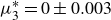 $\mu _{3}^{*} = 0 \pm 0.003$
,
$\mu _{3}^{*} = 0 \pm 0.003$
,
 $A_{3} = -0.05 \pm 0.005$
,
$A_{3} = -0.05 \pm 0.005$
,
 $\alpha _{3} = 0.43 \pm 0.07$
. (b) First (blue) and second (orange) normal stress differences obtained in DEM simulations as a function of the inertial number. The blue and orange dashed lines show the fits of the power law (B2), leading to
$\alpha _{3} = 0.43 \pm 0.07$
. (b) First (blue) and second (orange) normal stress differences obtained in DEM simulations as a function of the inertial number. The blue and orange dashed lines show the fits of the power law (B2), leading to
 $N_{1}^{*} = 0.01 \pm 0.01$
,
$N_{1}^{*} = 0.01 \pm 0.01$
,
 $B_{1} = -0.26 \pm 0.03$
,
$B_{1} = -0.26 \pm 0.03$
,
 $\beta _{1} = 0.46 \pm 0.08$
and
$\beta _{1} = 0.46 \pm 0.08$
and
 $N_{2}^{*} = -0.1 \pm 0.01$
,
$N_{2}^{*} = -0.1 \pm 0.01$
,
 $B_{2} = -0.2 \pm 0.015$
,
$B_{2} = -0.2 \pm 0.015$
,
 $\beta _{2} = 0.37 \pm 0.06$
. (c) The
$\beta _{2} = 0.37 \pm 0.06$
. (c) The
 $C$
constant as a function of the inertial number computed using the exact expression (4.11) (blue) and by setting
$C$
constant as a function of the inertial number computed using the exact expression (4.11) (blue) and by setting
 $N_{1} = 0$
or equivalently
$N_{1} = 0$
or equivalently
 $\mu _{3} = 0$
(orange). In both panels, the filled circles are the simulations presented in this article, and the empty squares are data obtained under linear shear by Kim & Kamrin (Reference Kim and Kamrin2023) with the same numerical parameters as used in this study. The grey shaded area shows the range of inertial numbers corresponding to our experiments.
$\mu _{3} = 0$
(orange). In both panels, the filled circles are the simulations presented in this article, and the empty squares are data obtained under linear shear by Kim & Kamrin (Reference Kim and Kamrin2023) with the same numerical parameters as used in this study. The grey shaded area shows the range of inertial numbers corresponding to our experiments.

As shown by the blue points in figure 11(b), the constant
 $C$
defined by (4.11) is slightly larger than unity (within
$C$
defined by (4.11) is slightly larger than unity (within
 $5\,\%$
) in the numerical simulations. From (4.12) and (4.13), the constant
$5\,\%$
) in the numerical simulations. From (4.12) and (4.13), the constant
 $C$
can also be expressed using the scaled normal stress differences as
$C$
can also be expressed using the scaled normal stress differences as
 \begin{equation} C = 1 + \frac {1}{3} (N_{1}^{(0)} - N_{2}^{(0)} ). \end{equation}
Then, to infer the value of
 $N_{2}$
from the experiments in § 6 using (4.36), one must either provide a value for
$N_{2}$
from the experiments in § 6 using (4.36), one must either provide a value for
 $N_{1}$
, or adopt an assumption removing the dependency in the first-normal stress difference. As
$N_{1}$
, or adopt an assumption removing the dependency in the first-normal stress difference. As
 $N_{1} \ll N_{2}$
for
$N_{1} \ll N_{2}$
for
 $I \lt 10^{-1}$
, one could simply set
$I \lt 10^{-1}$
, one could simply set
 $N_{1} = 0$
in (4.11). As shown by the orange points in figure 11(b), this provides a good approximation until
$N_{1} = 0$
in (4.11). As shown by the orange points in figure 11(b), this provides a good approximation until
 $I \simeq 10^{-1}$
. For larger values of the inertial number,
$I \simeq 10^{-1}$
. For larger values of the inertial number,
 $N_{1}$
is not negligible anymore but of the same order of magnitude as
$N_{1}$
is not negligible anymore but of the same order of magnitude as
 $N_{2}$
, which leads to a large difference with the exact value of
$N_{2}$
, which leads to a large difference with the exact value of
 $C$
. Hence, a better approximation at larger inertial number is
$C$
. Hence, a better approximation at larger inertial number is
 $(N_{1} - N_{2})/3 \ll 1$
, hence
$(N_{1} - N_{2})/3 \ll 1$
, hence
 $C \approx 1$
, which keeps the error within
$C \approx 1$
, which keeps the error within
 $5\,\%$
.
$5\,\%$
.


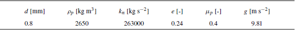
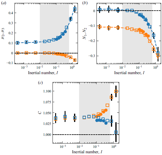


 Open access