


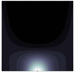



1. Introduction
Very few studies have investigated the effect of free-surface waves on heat transfer in the oceanic environment. In oceanography it is well established that convection and diffusion of heat in the free-surface boundary layer have important consequences for air–sea exchange processes. For example, Szeri (Reference Szeri1997) investigated heat transfer effects related to capillary waves, Szeri (Reference Szeri2017) focused on heat exchange across a turbulent liquid–gas interface and Witting (Reference Witting1971) and O'Brien (Reference O'Brien1967) considered simple irrotational progressive oscillations and Gerstner waves. Hetsroni, Mosyak & Yarin (Reference Hetsroni, Mosyak and Yarin1997) demonstrated experimentally that surface waves can have a significant effect on natural convection. Recent observations have shown that ocean waves could be more important in facilitating heat transport than originally believed (Veron, Melville & Lenain Reference Veron, Melville and Lenain2008).
Thermal conduction in fluids is a thoroughly researched field, with many of its theoretical aspects described by Landau & Lifshitz (Reference Landau and Lifshitz1989), Schlichting (Reference Schlichting1979) and White (Reference White1991). The temperature distribution in a moving fluid is strongly dependent on local flow characteristics, with a rapid variation in temperature occurring in the boundary layer close to a solid surface where the velocity gradient is significant. Lighthill (Reference Lighthill1950) provides a detailed discussion of heat transfer properties in a laminar boundary layer. In fluid flow the mechanism of heat diffusion is similar to that of mass diffusion. Applications of heat and mass transfer driven by oscillatory flows are described by Knobloch & Merryfield (Reference Knobloch and Merryfield1992) and Chatwin (Reference Chatwin1975), whereas studies of the dynamics of contaminants and other particles in the presence of ocean waves are given by Mei & Chian (Reference Mei and Chian1994) and Winckler, Liu & Mei (Reference Winckler, Liu and Mei2013).
To date, most studies have been restricted to simplified wave fields that do not replicate the complex hydrodynamics in the ocean. In this paper we develop a mathematical theory to analyse heat transfer through the seabed boundary layer, when forced by free-surface flow. Our model is based on the solution of the convection–diffusion equation for the temperature field in an incompressible liquid, when the velocity field is decoupled from the fluid temperature. We consider heat sources located at the ocean bed, and so the velocity components can be derived by a procedure analogous to that for seabed mass transport (Mei, Stiassnie & Yue Reference Mei, Stiassnie and Yue2005).
Recently, Michele, Stuhlmeier & Borthwick (Reference Michele, Stuhlmeier and Borthwick2021) investigated the temperature field generated by an infinitely long heat source of constant temperature beneath unidirectional waves. In the present work we include the effect of heat sources characterised by a more general class of temperature distributions, e.g. a source of finite length, of Gaussian shape, and multiple sources. We also consider the effects of prescribed heat flux seabed profiles that permit investigation of practical configurations including seabed heat sources between zones of insulating material as examined by Pedley (Reference Pedley1972a). In regular waves, the mean flow profile in the boundary layer is unidirectional and parallel to the seabed but still has a complicated vertical dependence. To better understand the physical phenomena involved, we derive several analytical expressions by means of Fourier integrals expressed in terms of complex Airy, Bessel and parabolic cylinder functions (cf. Gradshteyn & Ryzhik Reference Gradshteyn and Ryzhik2007). These solutions are based on simplified velocity profiles and allow us to obtain good agreement compared with numerical solutions based on a Crank–Nicholson implicit scheme (Smith Reference Smith1985). We also analyse the effect of standing waves caused by incident wave reflection from a vertical structure, such as a sea wall, which significantly complicates the expressions for convective terms. Our results suggest that it is necessary to extend present-day models of ocean heat transfer processes to include surface wave effects, especially when such models are applied to practical problems in ocean engineering and oceanography where analysis of temperature propagation is essential, such as sea-water conditioning (Hunt, Byers & Sánchez Reference Hunt, Byers and Sánchez2019), biofouling (Melo & Bott Reference Melo and Bott1997; Tiron et al. Reference Tiron, Gallagher, Doherty, Reynaud, Dias, Mallon and Whittaker2013; Yang et al. Reference Yang, Ringsberg, Johnson and Hu2017; Vinagre et al. Reference Vinagre, Simas, Cruz, Pinori and Svenson2020), underwater data centres (Cutler et al. Reference Cutler, Fowers, Kramer and Peterson2017), coral reefs (Ferrario et al. Reference Ferrario, Beck, Storlazzi, Micheli, Shepard and Airoldi2014) and satellite data calibration (Emery et al. Reference Emery, Baldwin, Schlussel and Reynolds2001).
Section 2 describes the governing equations for the flow field and heat transfer in a two-dimensional idealisation of the seabed laminar boundary layer. Section 3 derives analytical solutions for rectangular and trapezoidal approximations of the horizontal Eulerian-mean flow (called uniform current and trapezoidal current throughout the paper), the thermal boundary layer thickness, and resulting sea bed temperature and heat flux distributions. Section 4 compares results from a numerical solver of the full equations against the analytical solutions for seabed heat sources under progressive and standing waves. The main findings are listed in § 5.
2. Governing equations
Consider a two-dimensional fluid domain  $\varOmega (x,z,t)$, where $x$ is the horizontal distance from a fixed origin, $z$ is the distance vertically upwards from a horizontal seabed and $t$ is time. For simplicity, we assume a seawater of constant density $\rho =1.00\times 10^3\ {\rm kg}\ {\rm m}^{-3}$, constant kinematic viscosity $\nu =1.00\times 10^{-6}\ {\rm m}^2\ {\rm s}^{-1}$ and constant thermometric conductivity $\chi =1.4 \times 10^{-7} \ {\rm m}^2\ {\rm s}^{-1}$. The seawater and seabed have an initial temperature $\mathcal {T}=\mathcal {T}_i$. The water temperature at a large distance from the heat source is fixed at $\mathcal {T}=\mathcal {T}_i$ for all time. For convenience, we make use of relative temperature $T=\mathcal {T}-\mathcal {T}_i$. The resulting equation for convection and diffusion of relative temperature $\mathcal {T}$ is written (Schlichting Reference Schlichting1979; Landau & Lifshitz Reference Landau and Lifshitz1989; White Reference White1991)
 \begin{equation} \frac{\partial T}{\partial t}+u\frac{\partial T}{\partial x}+w\frac{\partial T}{\partial z}=\chi \left(\frac{\partial^2 T}{\partial x^2}+\frac{\partial^2 T}{\partial z^2}\right),\end{equation}
where  $(u,w)$ are horizontal and vertical components of the velocity field.
The fluid properties are assumed constant and independent of temperature. This is reasonable solely for small variations in  $T$, and so the theory is valid provided $T\sim O(10)\,^{\circ} {{\rm C}}$ and the initial fluid temperature $\mathcal {T}_i$ is far from freezing or boiling points (White Reference White1991).
As outlined by Michele et al. (Reference Michele, Stuhlmeier and Borthwick2021), diffusion effects become significant in the boundary layer where fluid viscosity is not negligible. In this work we consider flat heat sources located along a horizontal seabed; therefore,  $(u,w)$ can be found by following a similar procedure analogous to that used in the analysis of mass transport (see e.g. Mei et al. Reference Mei, Stiassnie and Yue2005, § 10.2). The next section derives expressions for the velocity components.
2.1. Flow field in the seabed laminar boundary layer
Let us assume the non-dimensional quantities
 \begin{align} x'=x k,\quad z'=\frac{z}{\delta},\quad u'=u \frac{\sinh(kh)}{A\omega},\quad w'=w\frac{\sinh(kh)}{A\omega k\delta},\quad t'=\omega t,\quad P'=\frac{P}{\rho g A}, \end{align}
and the small parameter denoting wave steepness
 \begin{equation} \epsilon=A k\ll1, \end{equation}
where  $k$ is the wavenumber, $\omega$ the angular frequency, $A$ the amplitude of the long-crested free-surface waves over constant water depth $h$,
$h$,  $P$ is total pressure and $\delta =\sqrt {2\nu /\omega }$ is the characteristic laminar boundary layer thickness. Non-dimensional continuity and Navier–Stokes equations are consequently given by (Mei et al. Reference Mei, Stiassnie and Yue2005)
 \begin{gather} \frac{\partial u'}{\partial x'}+\frac{\partial w'}{\partial z'}=0,\end{gather}
 \begin{gather} \frac{\partial u'}{\partial t'}+\frac{\epsilon}{\sinh(kh)}\left(u'\frac{\partial u'}{\partial x'}+w'\frac{\partial u'}{\partial z'}\right)={-}\frac{gk\sinh{(kh)}}{\omega^2}\frac{\partial P'}{\partial x'}+\frac{1}{2}\left(\delta^2k^2\frac{\partial^2 u'}{\partial x'^2}+\frac{\partial^2 u'}{\partial z'^2}\right),\end{gather}
 \begin{gather} \frac{\partial w'}{\partial t'}+\frac{\epsilon}{\sinh(kh)}\left(u'\frac{\partial w'}{\partial x'}+w'\frac{\partial w'}{\partial z'}\right)={-}\frac{g\sinh{(kh)}}{A\omega^2 k\delta}\left(\frac{A}{\delta}\frac{\partial P'}{\partial z'}+1\right)\nonumber\\ +\frac{1}{2}\left(\delta^2k^2\frac{\partial^2 w'}{\partial x'^2}+\frac{\partial^2 u'}{\partial z'^2}\right). \end{gather}
 In a typical ocean, the depth  $h\sim O(10)$ m, wave amplitude $A\sim O(1)$ m, wavelength $O(10)$ m and frequency $\omega \sim O(1)\ {\rm rad} {\rm s}^{-1}$, in which case $k\sim O(10^{-1})\ {\rm m}^{-1}$, $\sinh {(kh)}\sim O(1)$, $\epsilon \sim O(10^{-1})$ and $\delta \sim O(10^{-3})$ m. Thus, $k\delta \sim O(10^{-4})\sim O(\epsilon ^4)$, and (2.5)–(2.6) reduce to
 $$\begin{gather} \frac{\partial u'}{\partial t'}+\frac{\epsilon}{\sinh(kh)}\left(u'\frac{\partial u'}{\partial x'}+w'\frac{\partial u'}{\partial z'}\right)={-}\frac{gk\sinh{(kh)}}{\omega^2}\frac{\partial P'}{\partial x'}+\frac{1}{2}\frac{\partial^2 u'}{\partial z'^2}+O(\epsilon^8), \end{gather}$$
 $$\begin{gather}g\sinh{(kh)}\left(\frac{A}{\delta}\frac{\partial P'}{\partial z'}+1\right)+O(\epsilon^4)=0. \end{gather}$$
The dynamic pressure  $p=P-\rho g z$ does not depend on $z$ and has the same value as in the inviscid field immediately above the boundary layer governed by the non-dimensional Euler equation
 \begin{equation} \frac{\partial U'}{\partial t'}+\frac{\epsilon}{\sinh(kh)}U'\frac{\partial U'}{\partial x'}={-}\frac{gk\sinh{(kh)}}{\omega^2}\frac{\partial p'}{\partial x'},\end{equation}
where  $U'=U\sinh (kh)/(A\omega )$ is the non-dimensional horizontal inviscid flow velocity at the top of the seabed boundary layer, and
 \begin{equation} U={\rm{Re}}\{U_0(x) {\rm e}^{-\mathrm{i}\omega t}\}. \end{equation}
Substitution of (2.9) into (2.7) yields
 \begin{equation} \frac{\partial u'}{\partial t'}+\frac{\epsilon}{\sinh(kh)}\left(u'\frac{\partial u'}{\partial x'}+w'\frac{\partial u'}{\partial z'}\right)=\frac{\partial U'}{\partial t'}+\frac{\epsilon}{\sinh(kh)}U'\frac{\partial U'}{\partial x'}+\frac{1}{2}\frac{\partial^2 u'}{\partial z'^2}+O(\epsilon^8),\end{equation}
which in dimensional form becomes
 \begin{equation} \frac{\partial u}{\partial t}+u\frac{\partial u}{\partial x}+w\frac{\partial u}{\partial z}=\frac{\partial U}{\partial t}+U\frac{\partial U}{\partial x}+\nu \frac{\partial^2 u}{\partial z^2}.\end{equation}
 By introducing the perturbation expansion  $\{u,w\}=\{u_1,w_1\}+\{u_2,w_2\}+O(\omega A\epsilon ^2)$ (with subscripts denoting orders in $\epsilon$), it is straightforward to obtain
 \begin{equation}
\left.\begin{gathered}
u_1={\rm{Re}}\{U_0 (1-{\rm e}^{-\left(1-\mathrm{i}\right)z'}){\rm
e}^{-\mathrm{i}\omega t}\},\\
w_1={\rm{Re}}\left\{\delta \frac{\mathrm{d}
U_0}{\mathrm{d}\kern0.7pt x}\left[\frac{1+\mathrm{i}}{2}(1-{\rm e}^{{-}z'(1-\mathrm{i})})-z' \right]{\rm
e}^{-\mathrm{i}\omega t}\right\}.
\end{gathered}\right\}\end{equation}
\begin{equation}
\left.\begin{gathered}
u_1={\rm{Re}}\{U_0 (1-{\rm e}^{-\left(1-\mathrm{i}\right)z'}){\rm
e}^{-\mathrm{i}\omega t}\},\\
w_1={\rm{Re}}\left\{\delta \frac{\mathrm{d}
U_0}{\mathrm{d}\kern0.7pt x}\left[\frac{1+\mathrm{i}}{2}(1-{\rm e}^{{-}z'(1-\mathrm{i})})-z' \right]{\rm
e}^{-\mathrm{i}\omega t}\right\}.
\end{gathered}\right\}\end{equation}
At second order,  $O(\epsilon )$, we obtain a second-harmonic ( $2\omega$) component and the Eulerian-mean flow, derived from the quadratic products in (2.12). The second-harmonic component contributes only a small oscillatory correction to the first-harmonic component and can be neglected when examining heat transfer. Conversely, the following Eulerian-mean flow associated with the zeroth-harmonic component contributes to temperature transfer at ${O}(1)$ (Mei et al. Reference Mei, Stiassnie and Yue2005),
 \begin{equation} \bar{u}_2={-}\frac{1}{\omega}{\rm{Re}}\left\{FU_0\frac{\mathrm{d} U_0^*}{\mathrm{d}\kern0.7pt x}\right\},\quad \bar{w}_2={-}\int_0^z\frac{\partial \bar{u}_2}{\partial x}\,\mathrm{d}z, \end{equation}
where the bar represents a time-averaged value,  $()^*$ denotes the complex conjugate, and
 \begin{equation} F=\frac{3\mathrm{i}-1}{2}{\rm e}^{z'(\mathrm{i}-1)}-\frac{\mathrm{i}}{2} {\rm e}^{{-}z'(\mathrm{i}+1)}-\frac{1+\mathrm{i}}{4}{\rm e}^{{-}2z'}+z'\frac{1+\mathrm{i}}{2} {\rm e}^{z'(\mathrm{i}-1)}+\frac{3}{4}(1-\mathrm{i}). \end{equation}
Consider an incident and reflected wave field described by the velocity potential and linear dispersion equation (Mei et al. Reference Mei, Stiassnie and Yue2005):
 \begin{equation} \varPhi={\rm{Re}}\left\{\frac{-\mathrm{i} A g}{\omega}\frac{\cosh{k z}}{\cosh{k h}}({\rm e}^{\mathrm{i}kx}+R{\rm e}^{-\mathrm{i}kx}){\rm e}^{-\mathrm{i}\omega t}\right\},\quad \omega^2=gk\tanh(kh), \end{equation}
where  $g$ is the acceleration due to gravity and $R$ is the reflection coefficient. Here, $R=1$ represents standing waves, whereas $R=0$ represents incident waves propagating in the positive $x$ direction. The spatial dependence of $U_0$ is thence given by
 \begin{align}
\left.U=\varPhi_x\right|_{z=0}={\rm{Re}}\left\{\frac{A
\omega}{ \sinh{(k h)}}({\rm e}^{\mathrm{i}kx}-R{\rm
e}^{-\mathrm{i}kx}){\rm e}^{-\mathrm{i}\omega
t}\right\}\rightarrow U_0=\frac{A \omega}{ \sinh{(k
h)}}({\rm e}^{\mathrm{i}kx}-R{\rm
e}^{-\mathrm{i}kx}).
\end{align}
\begin{align}
\left.U=\varPhi_x\right|_{z=0}={\rm{Re}}\left\{\frac{A
\omega}{ \sinh{(k h)}}({\rm e}^{\mathrm{i}kx}-R{\rm
e}^{-\mathrm{i}kx}){\rm e}^{-\mathrm{i}\omega
t}\right\}\rightarrow U_0=\frac{A \omega}{ \sinh{(k
h)}}({\rm e}^{\mathrm{i}kx}-R{\rm
e}^{-\mathrm{i}kx}).
\end{align}
Substituting (2.17) into (2.13)–(2.14a,b) gives the following expressions for the horizontal and vertical fluid velocity components in the boundary layer up to second order:
 \begin{align}
u&=\frac{A\omega}{\sinh{(kh)}}\nonumber\\ &\quad\times{\rm{Re}}\left\{ ({\rm
e}^{\mathrm{i}kx}-R{\rm e}^{-\mathrm{i}kx})
(1-{\rm e}^{-\left(1-\mathrm{i}\right)z'}){\rm
e}^{-\mathrm{i}\omega t}+\epsilon\frac{\mathrm{i}
F}{\sinh{(kh)}}(1-R^2+2\mathrm{i}R
\sin{(2kx)})\right\},
\end{align}
\begin{align}
u&=\frac{A\omega}{\sinh{(kh)}}\nonumber\\ &\quad\times{\rm{Re}}\left\{ ({\rm
e}^{\mathrm{i}kx}-R{\rm e}^{-\mathrm{i}kx})
(1-{\rm e}^{-\left(1-\mathrm{i}\right)z'}){\rm
e}^{-\mathrm{i}\omega t}+\epsilon\frac{\mathrm{i}
F}{\sinh{(kh)}}(1-R^2+2\mathrm{i}R
\sin{(2kx)})\right\},
\end{align}
 \begin{align} w&=\frac{A\delta k
\omega}{ \sinh{(k h)}}\nonumber\\ &\quad
\times{\rm{Re}}\left\{\mathrm{i} ({\rm
e}^{\mathrm{i}kx}+R{\rm
e}^{-\mathrm{i}kx})\left[\frac{1+\mathrm{i}}{2}(1-
{\rm
e}^{{-}z'\left(1-\mathrm{i}\right)})-z'\right]{\rm
e}^{-\mathrm{i}\omega
t}+\epsilon\frac{4R\cos{(2kx)}}{\delta
\sinh{(kh)}}\int_0^zF\,\mathrm{d}z\right\}.
\end{align}
\begin{align} w&=\frac{A\delta k
\omega}{ \sinh{(k h)}}\nonumber\\ &\quad
\times{\rm{Re}}\left\{\mathrm{i} ({\rm
e}^{\mathrm{i}kx}+R{\rm
e}^{-\mathrm{i}kx})\left[\frac{1+\mathrm{i}}{2}(1-
{\rm
e}^{{-}z'\left(1-\mathrm{i}\right)})-z'\right]{\rm
e}^{-\mathrm{i}\omega
t}+\epsilon\frac{4R\cos{(2kx)}}{\delta
\sinh{(kh)}}\int_0^zF\,\mathrm{d}z\right\}.
\end{align}
The first term inside the curly brackets corresponds to the leading-order solution with the same frequency as the free-surface waves. The second term represents the time-independent Eulerian-mean flow. This is smaller in magnitude than the first term, but is responsible for the slow time evolution of the thermal boundary layer thickness (as shown in the next section). Therefore, the second term plays a major role in seabed heat transfer.
The flow described by the analytical model developed herein should satisfy criteria for laminar stability of the seabed boundary layer. For example, Jonsson (Reference Jonsson1966), Blondeaux & Vittori (Reference Blondeaux and Vittori1994), Verzicco & Vittori (Reference Verzicco and Vittori1996) and Vittori & Verzicco (Reference Vittori and Verzicco1998) found disturbed laminar regimes to occur in the range  $R_\delta \sim {O}(100)\unicode{x2013} {O}(500)$, where $R_\delta =A\omega \delta /[\nu \sinh (kh)]$ is defined as the Reynolds number in the boundary layer. The foregoing authors found that intermittently turbulent oscillations appear for $R_\delta >{O}(500)$. Blondeaux, Pralits & Vittori (Reference Blondeaux, Pralits and Vittori2021) recently developed a linearised theory for stability analysis of the seabed boundary layer beneath propagating waves and considered the combined effects of harmonic oscillations, a second-harmonic response and a steady Eulerian-mean flow. Blondeaux et al. (Reference Blondeaux, Pralits and Vittori2021) found a first critical value of $R_\delta \sim {O}(100)$ but did not identify a criterion to distinguish between the disturbed laminar and intermittently turbulent regimes as in the case of Stokes boundary layers analysed by Blondeaux & Vittori (Reference Blondeaux and Vittori2021).
Jensen, Sumer & Fredsøe (Reference Jensen, Sumer and Fredsøe1989) defined the Reynolds number as  $\textit {Re}=aU_{0m}/\nu$, where $U_{0m}$ is the maximum value of the free-stream velocity and $a$ is the amplitude of the free-stream motion and equal to $U_{0m}/ \omega$ when the free-stream velocity varies sinusoidally with time. Jensen et al. (Reference Jensen, Sumer and Fredsøe1989) showed that the critical value corresponding to the onset of turbulence is approximately $\textit {Re}\simeq 10^5$. In our work the free-stream velocity corresponds to the outer velocity just above the seabed boundary layer $A\omega /\sinh (kh)$; hence, the Reynolds number introduced by Jensen et al. (Reference Jensen, Sumer and Fredsøe1989) can be equivalently defined as $\textit {Re}=A^2\omega /[\nu \sinh ^2(kh)]=R_{\delta }^2/2$.
The preceding criteria suggest that the range of applications of our proposed laminar flow model should satisfy  $R_\delta < O(500)$. However, the effect of heated water might have a strong stabilising effect, as also reported by White (Reference White1991) and Schlichting (Reference Schlichting1979). In water, wall heating delays the onset of growth of Tollmien–Schlichting disturbances, and the critical Reynolds number can increase significantly. Experimental and theoretical analyses reported by Wazzan, Okamura & Smith (Reference Wazzan, Okamura and Smith1968) and Stratizar, Reshokto & Prahl (Reference Stratizar, Reshokto and Prahl1977) confirm this. For the foregoing reasons, we can infer that wave fields where $R_\delta <500$, when combined with temperature stratification due to heat transfer, yield reasonably stable laminar boundary layers. A stability analysis similar to that developed by Blondeaux et al. (Reference Blondeaux, Pralits and Vittori2021) would be needed to confirm this statement, and is a topic worthy of future investigation.
Taking  $h=5$ m, $A=0.25$ m and $\omega =1.5\ \textrm {rad}\ \textrm {s}^{-1}$ we obtain $R_\delta =248$ and $\textit {Re}=3.08\times 10^4$, whereas for the smaller frequency $\omega =1\ \textrm {rad}\ \textrm {s}^{-1}$, we obtain $R_\delta =409$ and $\textit {Re}=8.4\times 10^4$; hence, the Reynolds number diminishes with increasing $\omega$. These values are smaller than the thresholds $R_\delta =500$, $\textit {Re}=10^5$ and laminar flow is likely.
We now examine the range of applicability of the present model. Figure 1 presents curves of wave amplitude  $A$ against wave frequency $\omega$ corresponding to the critical values $R_\delta =500$ (figure 1a), $\textit {Re}=10^5$ (figure 1b), for different depths $h=[2.5; 5; 7.5; 10]$ m. For a fixed value of $h$, the conditions of laminar flow stability are satisfied by $A$ and $\omega$ values located to the right-hand side of the corresponding curve. At larger depths and frequencies the laminar flow becomes more stable.
Curves of surface elevation amplitude  $A$ with wave frequency $\omega$, for different water depths corresponding to the thresholds: (a) $R_\delta =500$ and (b) $\textit {Re}=10^5$. For a given value of $h$, the laminar flow is stable provided $A$ and $\omega$ are located to the right of the relevant curve.

2.2. Heat transfer in the boundary layer
The thermal boundary layer thickness  $\delta _T$ differs from the viscous boundary layer thickness $\delta$, and is strongly affected by the velocity component profile (derived in the previous section). In order to investigate the behaviour of $\delta _T$ we define the following non-dimensional variables:
 \begin{equation} \zeta'=\frac{z}{\delta_T},\quad T'=\frac{T}{\varDelta_T}. \end{equation}
Here the scale for  $z$ is now the thermal boundary layer thickness $\delta _T$, and $\varDelta _T=\mathcal {T}_b-\mathcal {T}_i$ is the relative heat source temperature, with $\mathcal {T}_b$ being the absolute heat source temperature. Substituting the above and (2.2a–f) into (2.1), we obtain the following governing equation in non-dimensional form:
 \begin{equation} \frac{\partial T'}{\partial t'}+\epsilon\left[\frac{u'}{\sinh{(kh)}}\frac{\partial T'}{\partial x'}+\frac{w'\delta}{\delta_T\sinh(kh)}\frac{\partial T'}{\partial \zeta'}\right]=\frac{\delta^2}{2\textit{Pr}}\left[\frac{1}{\delta_T^2}\frac{\partial^2 T'}{\partial \zeta'^2}+k^2\frac{\partial^2 T'}{\partial x'^2}\right]. \end{equation}
Here  $\textit {Pr}=\nu /\chi \sim 7$ is the Prandtl number defined as the ratio of momentum diffusivity to thermal diffusivity for seawater. By assuming $\delta _T\geqslant \delta$, and $\sinh (kh)\geqslant O(1)$, then from (2.21) we find that $\partial T'/\partial t'$ is much larger than the other terms, i.e. $\partial T'/\partial t'\sim 0$. This means that the temperature at leading order is a function of spatial coordinates and a slow time scale only, and that the slow evolution of thermal boundary layer thickness is solely affected by the time-independent Eulerian-mean flow components $(\bar {u}_2,\bar {w}_2)$. Therefore, by assuming $T'$ to be a slowly varying function of time and then averaging with respect to the fast time scale (Jordan & Smith Reference Jordan and Smith2011), we obtain the governing equation of fluid temperature (in dimensional variables) as
 \begin{equation} \frac{\partial T}{\partial t}+\bar{u}_2\frac{\partial T}{\partial x}+\bar{w}_2\frac{\partial T}{\partial z}=\chi \frac{\partial^2 T}{\partial z^2},\end{equation}
where the term  $\chi \partial ^2 T/\partial x^2\sim O(\delta ^2k^2/(2\textit {Pr}))\sim O(\epsilon ^9)$ is assumed negligible with respect to the other quantities. Equation (2.22) describes the temperature field within the boundary layer and governs the slow evolution of $\delta _T$.
Note that the effect of fast oscillatory components (2.13) does not appear in the governing equation (2.22) because of the scales (2.2a–f) and fast time averaging. Smaller spatial scales allow the convective and diffusion terms to be leading-order terms, and both  $\partial T'/\partial t'\sim 0$ at $O(1)$ and (2.22) would no longer be valid. We further point out that significant benefits accrue from using (2.22) which is considerably simpler than (2.1). The absence of time-dependent components $(u_1,w_1)$ and horizontal temperature diffusion enables us to reduce significantly the difficulty of the problem and obtain the analytical solutions reported in § 3.
In the present work we will consider the effects of (1) a prescribed seabed temperature (Dirichlet boundary condition) and (2) a prescribed seabed heat flux (Neumann boundary condition). The case with a Dirichlet boundary condition (1) can be stated as follows. At time  $t=0$, the temperature of a finite length of seabed $S_b$ increases instantaneously to $\mathcal {T}_b(x)>\mathcal {T}_i$ and remains constant thereafter. Otherwise, the temperature of the seabed is fixed at $\mathcal {T}_i$ for all time. We obtain
 $$\begin{gather} \frac{\partial T}{\partial t}+\bar{u}_2\frac{\partial T}{\partial x}+ \bar{w}_2\frac{\partial T}{\partial z}=\chi \frac{\partial^2 T}{\partial z^2},\quad \varOmega(x,z,t), \end{gather}$$
 $$\begin{gather}T=\varDelta_T, \quad x\in S_b,\ t>0, \end{gather}$$
 $$\begin{gather}T=0, \quad x\in(-\infty,+\infty)\setminus S_b,\ t>0, \end{gather}$$
 $$\begin{gather}T=0, \quad \sqrt{x^2+z^2}\rightarrow\infty,\ t>0, \end{gather}$$
 $$\begin{gather}T=0, \quad \varOmega(x,z,0). \end{gather}$$
This configuration is equivalent to a heat source with prescribed temperature and a seabed of much larger thermal conductivity than water, therefore, the temperature remains uniform at the solid boundary and equal to  $\mathcal {T}_i$.
Similarly, the case with a Neumann boundary condition (2) can be stated as follows. At time  $t=0$, the heat flux through a finite length section of seabed $S_b$ increases instantaneously to $\mathcal {F}(x)>0$ and remains constant thereafter. The heat flux through the remainder of the insulated seabed is zero at all times. From Fourier's law we obtain
 $$\begin{gather} \frac{\partial T}{\partial t}+\bar{u}_2\frac{\partial T}{\partial x}+\bar{w}_2\frac{\partial T}{\partial z}=\chi \frac{\partial^2 T}{\partial z^2},\quad \varOmega(x,z,t), \end{gather}$$
 $$\begin{gather}\frac{\partial T}{\partial z}={-}\frac{\mathcal{F}}{\kappa} , \quad x\in S_b,\ t>0, \end{gather}$$
 $$\begin{gather}\frac{\partial T}{\partial z}=0, \quad x\in(-\infty,+\infty)\setminus S_b,\ t>0, \end{gather}$$
 $$\begin{gather}T=0, \quad \sqrt{x^2+z^2}\rightarrow\infty,\ t>0, \end{gather}$$
 $$\begin{gather}T=0, \quad \varOmega(x,z,0), \end{gather}$$
where  $\kappa =\chi \rho c_p$ is thermal conductivity and $c_p$ is specific heat at constant pressure. Practically speaking, the foregoing problem represents a heat source surrounded by seabed made of insulating material. A similar problem is analysed by Pedley (Reference Pedley1972a).
Solutions of (2.23)–(2.27) and (2.28)–(2.32) can easily be found by applying the Crank–Nicholson implicit numerical scheme (see also Smith Reference Smith1985; Mei et al. Reference Mei, Li, Michele, Sammarco and McBeth2021). However, analytical solutions are not straightforward to obtain because the convective terms  $(\bar {u}_2,\bar {w}_2)$ have complicated spatial dependence; therefore, solution of the foregoing governing equation is not an easy task and approximations are necessary. The following section investigates the effect of simplified velocity profiles on the thermal boundary layer over flat heat sources characterised by different temperature and heat flux distributions.
3. Approximate solutions for the mean flow and thermal boundary layer
In this section we determine approximate closed-form solutions to both problems (1) and (2) for propagating waves ( $R=0$). Even in the simple case of $R=0$, the horizontal component $\bar {u}_2$ has complicated vertical dependence, and so we utilise approximate velocity profiles to obtain an explicit solution. We first consider uniform horizontal flow of constant velocity $\bar {u}$ that is set equal to the Eulerian-mean flow at large distance from the seabed,
 \begin{equation} \bar{u}=\lim_{z\rightarrow\infty}\bar{u}_2=\epsilon\frac{3A \omega }{4\sinh^2(kh)}.\end{equation}
 The second velocity profile  $\bar {u}_{trap}$ resembles (2.14a,b) and is a trapezoidal approximation of the horizontal Eulerian-mean velocity (Schlichting Reference Schlichting1979)
 \begin{equation} \bar{u}_{trap}=\begin{cases} \displaystyle z\bar{u}^{(1)}=\epsilon z\frac{A \omega }{2\delta\sinh^2(kh)}, & \displaystyle 0< z<\frac{3\delta}{2}, \\[10pt] \displaystyle \bar{u}^{(2)}=\epsilon\frac{3A \omega }{4\sinh^2(kh)}, & \displaystyle z>\frac{3\delta}{2}, \end{cases} \end{equation}
where superscripts  $(1)$ and $(2)$ refer to the intervals $0< z<{3\delta }/{2}$ and $z>{3\delta }/{2}$, respectively. Note $\bar {u}^{(1)}$ does not have dimensions of velocity.
Figure 2 compares the approximate horizontal velocity profiles  $\bar {u}$ (3.1) and $\bar {u}_{trap}$ (3.2) to the complete expression $\bar {u}_2$ (2.14a,b) for typical parameter values, namely $\omega =1\ \textrm {rad}\ \textrm {s}^{-1}$, $A=0.25$ m and $h=5$ m. The $\bar {u}_{trap}$ and $\bar {u}_2$ profiles are qualitatively similar except for a small overshoot at $z\sim 3\delta /2$, which is not captured by the trapezoidal profile.


Table 1 summarises all the cases considered in this section. For each case, we find an analytical solution of practical interest. (Note that Michele et al. (Reference Michele, Stuhlmeier and Borthwick2021) limited their study to a single configuration and found a steady-state solution solely for linearly varying flow velocity profiles.) The uniform flow case is solved for unsteady conditions, whereas the trapezoidal flow case is solved solely for steady conditions. As will be shown in § 4, the latter turns out to be a very good approximation in regular progressive waves where  $R=0$. The section also considers the effects of different seabed distributions of Gaussian temperature and heat fluxes. (Please note that none of the solutions obtained for the cases in table 1 have been reported by Michele et al. (Reference Michele, Stuhlmeier and Borthwick2021) and Pedley (Reference Pedley1972a,Reference Pedleyb, Reference Pedley1975).)
Cases analysed for progressive regular waves ( $R=0$).

The analytical expressions derived in this section are used later to verify convergence of the numerical Crank–Nicholson scheme based on the complete velocity components (2.14a,b).
3.1. Heat transfer in uniform flow above the seabed
Let us consider the (vertically) uniform horizontal current  $\bar {u}$ (3.1) flowing above a flat heated surface of length $L$. This configuration is a simplified version of the unsteady heat transfer problem in the presence of constant streaming forced by propagating waves ( $R=0, \bar {w}_2=0$).
3.1.1. Case 1 – rectangular distribution of seabed temperature
Assuming a heat source of fixed temperature  $\varDelta _T$ and length $L$, the unsteady boundary value problem becomes
 $$\begin{gather} \frac{\partial T}{\partial t}+\bar{u}\frac{\partial T}{\partial x}=\chi\frac{\partial^2 T}{\partial z^2},\quad \varOmega(x,z,t), \end{gather}$$
 $$\begin{gather}T=\varDelta_T\left(H[x]-H[x-L]\right), \quad z=0, \end{gather}$$
 $$\begin{gather}T=0, \quad \sqrt{x^2+z^2}\rightarrow\infty, \end{gather}$$
 $$\begin{gather}T=0, \quad \varOmega(x,z,0), \end{gather}$$
where  $H$ is the Heaviside step function. (It should be noted that Pedley (Reference Pedley1972a,Reference Pedleyb, Reference Pedley1975) obtained an analytical solution to a similar problem.) By utilising a moving coordinate system such that $\xi =x-\bar {u}t$, with the Fourier sine transform and its inverse (Mei Reference Mei1997) the solution is
 \begin{align} T&=\varDelta_T\left\{\text{Erfc}\left[z\sqrt{\frac{\bar{u}}{4\chi x}}\right]-H\left[x-L\right]\text{Erfc}\left[z\sqrt{\frac{\bar{u}}{4\chi (x-L)}}\right]\right.\nonumber\\ &\quad +H\left[x-\bar{u}t\right]\left(\text{Erf}\left[z\sqrt{\frac{\bar{u}}{4\chi x}}\right]-\text{Erf}\left[\frac{z}{\sqrt{4\chi t}}\right]\right)\nonumber\\ &\quad \left.+H\left[x-\bar{u}t-L\right]\left(\text{Erf}\left[\frac{z}{\sqrt{4\chi t}}\right]-\text{Erf}\left[z\sqrt{\frac{\bar{u}}{4\chi (x-L)}}\right]\right)\right\}, \end{align}
where  $\textrm {Erf}$ and $\textrm {Erfc}$ represent the error function and the complementary error function, respectively (Abramowitz & Stegun Reference Abramowitz and Stegun1972). The physical meaning of each term in (3.7) is as follows: the first and third terms represent the unsteady temperature field above the heat source in the region $0< x< L$, the second and fourth terms represent the unsteady component elsewhere, namely in the region $x>L$. Of interest is the steady solution at very large time $T(x,z,t\rightarrow \infty )$, which is given by
 \begin{equation} T=\varDelta_T\left\{\text{Erfc}\left[z\sqrt{\frac{\bar{u}}{4\chi x}}\right]-H\left[x-L\right]\text{Erfc}\left[z\sqrt{\frac{\bar{u}}{4\chi (x-L)}}\right]\right\}.\end{equation}
 By analogy to laminar viscous boundary layer theory, the thermal boundary layer thickness  $\delta _T$ is defined as the thickness for which the water temperature is 1 % of the heat source temperature $\varDelta _T$, and can be estimated from (3.8) giving
 \begin{equation} \text{Erfc}\left[\delta_T\sqrt{\frac{\bar{u}}{4\chi x}}\right]=0.01 \rightarrow\ \delta_T\sim 3.64\times \sqrt{\frac{\chi x}{\bar{u}}}. \end{equation}
From the horizontal velocity component (3.1), we obtain
 \begin{equation} \delta_T\approx 4.2\times \sqrt{\frac{\chi \sinh^2(kh) x}{A\omega\epsilon}}.\end{equation}
In the ocean typically  $h={O}(10)$ m, $A\sim {O}(1)$ m, $\omega ={O}(1)\ \textrm {rad}\ \textrm {s}^{-1}$, $Lk\sim O(1)$ m and $x\sim L$, and we obtain $\delta _T\sim {O}(10^{-2})$ m. In other words, $\delta _T\gg \delta$. An explicit expression for $\delta _T$ in shallow water $kh\ll 1$ can also be determined as
 \begin{equation} \frac{\delta_T}{\delta}\sim kh\sqrt\frac{x}{A\epsilon}.\end{equation}
In deep water  $kh\gg 1$, and
 \begin{equation} \frac{\delta_T}{\delta}\sim e^{kh}\sqrt{\frac{x}{A\epsilon}},\end{equation}
indicating that the thermal boundary layer thickness is much larger in deep water than in shallow water.
As an example, we consider steady-state temperature fields (3.8) obtained for water depth  $h=5$ m, wave amplitude $A=0.25$ m, heat source temperature $\varDelta _T=10\,^{\circ }\textrm {C}$, heat source length $L=5$ m and two values of wave frequency $\omega =1\ \textrm {rad} \ \textrm {s}^{-1}$ and $1.5\ \textrm {rad}\ \textrm {s}^{-1}$. The resulting flow speed is $\bar {u}=[0.0098;0.0061]\ \textrm {m}\ \textrm {s}^{-1}$. Note that these parameters satisfy the criteria for laminar flow stability depicted in figure 1.
Figure 3 displays the steady-state temperature fields for  $\omega =1\ \textrm {rad}\ \textrm {s}^{-1}$ and $\omega =1.5\ \textrm {rad}\ \textrm {s}^{-1}$. It can be seen that $\delta _T\sim {O}(10^{-2})$ m at $x=L=5$ m, as predicted by (3.10). Specifically, the growth of $\delta _T$ is very rapid (in $x$) and slows down as $x$ increases. Note that as $\omega$ increases, the velocity above the plate decreases and the thermal boundary layer expands vertically.
Case 1, near-bed steady-state temperature fields for a uniform current profile  $\bar {u}$ and a prescribed seabed heat source where $\varDelta _T=10\,^{\circ} \textrm {C}$, $L=5$ m, $h=5$ m and $A=0.25$ m. Wave frequency: (a) $\omega =1\ \textrm {rad}\ \textrm {s}^{-1}$ and (b) $\omega =1.5\ \textrm {rad}\ \textrm {s}^{-1}$. Note that $\delta _T\sim {O}(10^{-2})$ m and increases with wave frequency as predicted by (3.10).

Figure 3 also shows that the temperature decays for large  $x$; therefore, the thermal boundary layer is also characterised by a horizontal width. This is of crucial significance when multiple heat sources are considered because they can interact with each other when the distance between them is sufficiently short. In order to characterize the temperature field for the seawater, we examine the location of the maximum of (3.8) for each $x$, which is obtained from
 \begin{equation} \frac{\partial T}{\partial z}=0\ \rightarrow\ z_{max}=\begin{cases} \displaystyle\sqrt{\frac{4\chi x(x-L)}{L\bar{u}}\log\left(\frac{\sqrt{x}}{\sqrt{x-L}}\right)} , & x>L,\\[10pt] 0, & x\in [0,L]. \end{cases}\end{equation}
 The maximum temperature coincides with the heat source ( $z_{max}=0$) for $x \leqslant L$ and its vertical elevation above the seabed increases monotonically with horizontal distance $x$ for $x>L$. By substituting (3.13) into (3.8) we obtain the following expression for maximum water temperature as a function of $x$:
$x$:
 \begin{align} T_{max}=\begin{cases} \displaystyle\varDelta_T\!\left\{\text{Erfc}\!\left[\sqrt{\frac{ x-L}{L}\log\left( \frac{\sqrt{x}}{\sqrt{x-L}}\right)}\right]-\text{Erfc}\!\left[\sqrt{\frac{ x}{L}\log\left(\frac{ \sqrt{x}}{\sqrt{x-L}}\right)}\right]\right\}, & x>L, \\[10pt] \varDelta_T, & x\in [0,L]. \end{cases} \end{align}
Surprisingly,  $T_{max}$ does not depend on fluid velocity $\bar {u}$ and thermal conductivity $\chi$, but only on heat source length $L$ and horizontal position $x$. Figure 4 shows the behaviour of the ratio $T_{max}/\varDelta _T$ as a function of distance from the right edge $(x-L)$ for different heat source lengths $L$. The longer the heat source, the slower the temperature decay. For example, when $L=5$ m, the maximum temperature is 10 % of $\varDelta _T$ after 10 m, as also shown in figure 3.
Ratio  $T_{max}/\varDelta _T$ as a function of distance $(x-L)$ from the edge of the heat source for different values of heat source length $L$.
$L$.

The unsteady seabed heat flux is evaluated from Fourier's law as follows:
 $$q = \left\{ {\matrix{ {} \hfill & {\kappa {\rm }\Delta _T\sqrt {\displaystyle{{\bar{u}} \over {x\pi \chi }}} \left[ {1 + \left( {\sqrt {\displaystyle{x \over {\bar{u}t}}} -1} \right)H\left[ {x-\bar{u}t} \right]} \right],} \hfill & {} \hfill & {x\in [0,L],} \hfill \cr {} \hfill & {\kappa {\rm }\Delta _T\sqrt {\displaystyle{{\bar{u}} \over {x\pi \chi }}} \left[ {1-\sqrt {\displaystyle{x \over {x-L}}} + \left( {\sqrt {\displaystyle{x \over {\bar{u}t}}} -1} \right)H\left[ {x-\bar{u}t} \right]} \right.} \hfill & {} \hfill & {} \hfill \cr {} \hfill & {\quad \left. { + \left( {\sqrt {\displaystyle{x \over {x-L}}} -\sqrt {\displaystyle{x \over {\bar{u}t}}} } \right)H\left[ {x-\bar{u}t-L} \right]} \right],} \hfill & {} \hfill & {x > L,} \hfill \cr {} \hfill & {0,} \hfill & {} \hfill & {x < 0.} \hfill \cr } } \right.$$
Expression (3.15a) is always positive and represents the heat flux exchanged between the heat source and the overlying seawater, whereas (3.15b) represents the negative heat flux in  $x>L$, beyond the heat source. Note that $q$ tends to infinity as $x^{-1/2}$ and $-(x-L)^{-1/2}$ for $x\rightarrow 0^+$ and $x\rightarrow L+0^+$, respectively, because of the discontinuous gradients in temperature at the edges of the heat source. Integrating (3.15a) and (3.15b), the total unsteady heat fluxes through the region $S_b$ and for $x>L$ are
 \begin{gather} Q_{S_b}=\int_{0}^Lq\,\mathrm{d}\kern0.7pt x=\begin{cases} \displaystyle\kappa \varDelta_T\frac{\bar{u}t+L}{\sqrt{{\rm \pi}\chi t}}, & t< L/\bar{u},\ x\in [0,L], \\[10pt] \displaystyle\kappa \varDelta_T\sqrt{\frac{4L\bar{u}}{\chi{\rm \pi}}}, & t>L/\bar{u},\ x\in [0,L], \end{cases}\end{gather}
 \begin{gather} Q_{x>L}=\int_{L}^\infty q\,\mathrm{d}\kern0.7pt x=\begin{cases} \kappa \varDelta_T\dfrac{\bar{u}t-2\sqrt{\bar{u}t(L+\bar{u}t)}} {\sqrt{{\rm \pi}\chi t}}, & t< L/\bar{u},\ x>L, \\[10pt] \kappa \varDelta_T\dfrac{L+2\bar{u}t-2\sqrt{\bar{u}t}(\sqrt{L}+\sqrt{L+\bar{u}t})} {\sqrt{{\rm \pi}\chi t}}, & t>L/\bar{u},\ x>L. \end{cases} \end{gather}
At steady state, the above expressions reduce to
 \begin{equation} \left.\begin{aligned} &\lim_{t\rightarrow\infty} Q_{S_b}=\kappa \varDelta_T\sqrt{\dfrac{4L\bar{u}}{\chi{\rm \pi}}}, x\in [0,L], \\ &\lim_{t\rightarrow\infty} Q_{x>L}={-}\kappa \varDelta_T\sqrt{\dfrac{4L\bar{u}}{\chi{\rm \pi}}},\quad x>L, \end{aligned}\right\}\end{equation}
with both attaining a maximum when  $\bar {u}$ is maximised, demonstrating that the wave-induced flow aids heat exchange. In addition, $Q_{S_b}$ and $Q_{x>L}$ have the same magnitude but opposite sign, and so the total amount of heat in the fluid domain remains constant at steady state (in accordance with the first law of thermodynamics).
3.1.2. Case 2 – rectangular distribution of seabed heat flux distribution
The heat flux is assumed equal to  $\mathcal {F}$ through $S_b$, and zero elsewhere. The boundary value problem has Neumann boundary conditions at the seabed, and is given by
 $$\begin{gather} \frac{\partial T}{\partial t}+\bar{u}\frac{\partial T}{\partial x} =\chi\frac{\partial^2 T}{\partial z^2},\quad \varOmega(x,z,t), \end{gather}$$
 $$\begin{gather}\frac{\partial T}{\partial z}={-}\frac{\mathcal{F}}{\kappa}\left(H[x]-H[x-L]\right), \quad z=0, \end{gather}$$
 $$\begin{gather}T=0, \quad \sqrt{x^2+z^2}\rightarrow\infty, \end{gather}$$
 $$\begin{gather}T=0, \quad \varOmega(x,z,0). \end{gather}$$
A solution is found using the moving coordinate  $\xi =x-\bar {u}t$, the Fourier cosine transform along $z$ and its inverse (Mei Reference Mei1997), giving
 \begin{align} T&=\frac{\mathcal{F}}{\kappa\sqrt{\rm \pi}}\left\{2\sqrt{\frac{x\chi}{\bar{u}}} \exp\left({-\frac{uz^2}{4x\chi}}\right)-z\sqrt{\rm \pi}\,\text{Erfc}\left[z\sqrt{\frac{\bar{u}}{4\chi x}}\right]\right.\nonumber\\ &\quad -H\left[x-L\right]\left(2\sqrt{\frac{(x-L)\chi}{\bar{u}}} \exp\left({-\frac{uz^2}{4\chi(x-L)}}\right)-z\sqrt{\rm \pi}\,\text{Erfc}\left[z\sqrt{\frac{\bar{u}}{4 \chi (x-L)}}\right]\right)\nonumber\\ &\quad +H\left[x-\bar{u}t\right]\left(2\sqrt{t\chi} \exp\left({-\frac{z^2}{4t\chi}}\right)-2\sqrt{\frac{x\chi}{\bar{u}}} \exp\left({-\frac{uz^2}{4\chi x}}\right)\right.\nonumber\\ &\quad \left.-z\sqrt{\rm \pi}\,\text{Erfc}\left[z\sqrt{\frac{\bar{u}}{4\chi x}}\right]- z\sqrt{\rm \pi}\,\text{Erfc}\left[\frac{z}{\sqrt{4\chi t}}\right]\right)\nonumber\\ &\quad -H\left[x-\bar{u}t-L\right]\left(2\sqrt{t\chi} \exp\left({-\frac{z^2}{4t\chi}}\right)-2\sqrt{\frac{(x-L)\chi}{\bar{u}}} \exp\left({-\frac{uz^2}{4\chi (x-L)}}\right)\right.\nonumber\\ &\quad \left.\left.+z\sqrt{\rm \pi}\,\text{Erfc}\left[z\sqrt{\frac{\bar{u}}{4\chi (x-L)}}\right]+z\sqrt{\rm \pi}\,\text{Erfc}\left[\frac{z}{\sqrt{4\chi t}}\right]\right)\right\}. \end{align}
The steady-state solution  $T(x,z,t\rightarrow \infty )$ becomes
 \begin{align} T&=\frac{\mathcal{F}}{\kappa\sqrt{\rm \pi}}\left\{2\sqrt{\frac{x\chi}{\bar{u}}} \exp\left({-\frac{uz^2}{4x\chi}}\right)-z\sqrt{\rm \pi}\,\text{Erfc}\left[z\sqrt{\frac{\bar{u}}{4\chi x}}\right]\right.\nonumber\\ &\quad-\left.H\left[x-L\right]\left(2\sqrt{\frac{(x-L)\chi}{\bar{u}}} \exp\left({-\frac{uz^2}{4\chi (x-L)}}\right)-z\sqrt{\rm \pi}\,\text{Erfc}\left[z\sqrt{\frac{\bar{u}}{4\chi (x-L)}}\right]\right)\right\}. \end{align}
Turning to the temperature profile at the seabed, from (3.24) we obtain
 \begin{equation} T(x,0,\infty)=\frac{2\mathcal{F}}{\kappa}\sqrt{\frac{\chi}{{\rm \pi}\bar{u}}}\left\{\sqrt{x} -H\left[x-L\right]\sqrt{x-L}\right\},\end{equation}
which has a maximum at  $x=L$, namely
 \begin{equation} T(L,0,\infty)=\frac{2\mathcal{F}}{\kappa}\sqrt{\frac{\chi L}{{\rm \pi}\bar{u}}}. \end{equation}
The foregoing gives an estimate of the temperature at the seabed for a fixed heat flux.
Given the Eulerian-mean velocity  $\bar {u}\sim O(10^{-2})\ \textrm {m}\ \textrm {s}^{-1}$ and the thermal conductivity of seawater $\kappa \sim 0.61\ \textrm {W}\ (\textrm {m}\,^{\circ }\textrm {C})^{-1}$, we obtain $T\sim 10^{-2}\mathcal {F}\sqrt {L}\,^{\circ} \textrm {C}$. The temperature field is determined by assuming $\mathcal {F}=10^3\ \textrm {W}\ \textrm {m}^{-2}$ and using the same parameters as in the previous section. Figure 5 depicts the steady-state temperature field for $\omega =1\ \textrm {rad}\ \textrm {s}^{-1}$ and $\omega =1.5\ \textrm {rad}\ \textrm {s}^{-1}$. The temperature contours above the heat source are similar to those in figure 3. To the right of the heat source ( $x>L$), the temperature decays more slowly than in case 1. This is due to the absence of heat flux directed towards the seabed for $x>L$.
Case 2: near-bed steady-state temperature fields for a uniform current  $\bar {u}$ profile and prescribed seabed heat flux $\mathcal {F}=10^3\ \textrm {W}\ \textrm {m}^{-2}$ where $L=5$ m, $h=5$ m and $A=0.25$ m. Wave frequency: (a) $\omega =1\ \textrm {rad}\ \textrm {s}^{-1}$ and (b) $\omega =1.5\ \textrm {rad}\ \textrm {s}^{-1}$. Above the heat source, the boundary layer thickness is similar to that of case 1 in figure 3, whereas for $x>L$, the temperature decay in the vertical is slower.

3.2. Heat transfer in trapezoidal flow over the seabed
A better approximation at steady state is achieved by assuming a trapezoidal profile  $\bar {u}_{trap}$ (3.2). We now apply this velocity profile to the generalized temperature and heat flux seabed profiles.
3.2.1. Case 3 – prescribed temperature distribution at the seabed
By adopting the approximate vertical profile  $\bar {u}_{trap}$ given by (3.2) and a general seabed temperature distribution $T_0(x)$, the steady boundary value problem can be written as
 $$\begin{gather} \bar{u}_{trap}\frac{\partial T}{\partial x}-\chi\frac{\partial^2 T}{\partial z^2}=0,\quad \varOmega(x,z), \end{gather}$$
 $$\begin{gather}T=T_0(x), \quad x\in S_b, \end{gather}$$
 $$\begin{gather}T=0, \quad \sqrt{x^2+z^2}\rightarrow\infty, \end{gather}$$
which is more complicated than the boundary value problem solved by Michele et al. (Reference Michele, Stuhlmeier and Borthwick2021) because of the stepped distribution of the heat source and the trapezoidal velocity profile. Furthermore, it is not possible to identify similarity solutions; instead, it is necessary to pursue a different approach.
Given that the water domain has infinite extent along  $x$, we define the Fourier transform $\tilde {T}$ and its inverse as (Mei Reference Mei1997)
 \begin{equation} \tilde{T}=\int_{-\infty}^{\infty} T(x,z){\rm e}^{-\mathrm{i}\alpha x}\,\mathrm{d}\kern0.7pt x,\quad T=\frac{1}{2{\rm \pi}}\int_{-\infty}^{\infty} \tilde{T}(\alpha,z){\rm e}^{\mathrm{i}\alpha x}\,\mathrm{d}\alpha.\end{equation}
The above expressions define the transformed problem for  $T$,
$T$,
 $$\begin{gather} \chi\frac{\mathrm{d}^2\tilde{T}}{\mathrm{d}z^2}=\mathrm{i}\alpha \bar{u}_{trap}\tilde{T},\quad \varOmega(\alpha,z), \end{gather}$$
 $$\begin{gather}\tilde{T}=\tilde{T}_0, \quad z=0, \end{gather}$$
 $$\begin{gather}\tilde{T}=0, \quad z\rightarrow\infty. \end{gather}$$
Noting that  $\bar {u}_{trap}$ has a discontinuous derivative, we decompose the problem in the vertical direction and enforce continuity of temperature and heat flux at the common boundary $z=3\delta /2$, giving
 $$\begin{gather} \chi\frac{\mathrm{d}^2\tilde{T}^{(1)}}{\mathrm{d}z^2}=\mathrm{i}\alpha z\bar{u}^{(1)}\tilde{T}^{(1)},\quad 0< z<\frac{3\delta}{2}, \end{gather}$$
 $$\begin{gather}\chi\frac{\mathrm{d}^2\tilde{T}^{(2)}}{\mathrm{d}z^2}= \mathrm{i}\alpha \bar{u}^{(2)}\tilde{T}^{(2)},\quad z>\frac{3\delta}{2}, \end{gather}$$
 $$\begin{gather}\tilde{T}^{(1)}=\tilde{T}_0, \quad z=0, \end{gather}$$
 $$\begin{gather}\tilde{T}^{(1)}=\tilde{T}^{(2)}, \quad z=\frac{3\delta}{2}, \end{gather}$$
 $$\begin{gather}\frac{\mathrm{d}\tilde{T}^{(1)}}{\mathrm{d}z}= \frac{\mathrm{d}\tilde{T}^{(2)}}{\mathrm{d}z}, \quad z=\frac{3\delta}{2}, \end{gather}$$
 $$\begin{gather}\tilde{T}^{(2)}=0, \quad z\rightarrow\infty. \end{gather}$$
Using (3.30a,b), the required solutions in integral form are
 $$\begin{gather} T^{(1)}\,{=}\,\frac{3^{2/3}\varGamma\left(\frac{2}{3}\right)}{\rm \pi}{\rm{Re}}\int_{0}^{\infty}\tilde{T}_0 \left\{c_1 \text{Ai}\!\left[z\left(\frac{\mathrm{i}\bar{u}^{(1)}\alpha}{\chi}\right)^{{1/3}}\right]{+}\,c_2 \text{Bi}\left[z\left(\frac{\mathrm{i}\bar{u}^{(1)}\alpha}{\chi}\right)^{{1/3}}\right]\right\} {\rm e}^{\mathrm{i}\alpha x} \,\mathrm{d}\alpha, \end{gather}$$
 $$\begin{gather}T^{(2)}=\frac{3^{2/3}\varGamma\left(\frac{2}{3}\right)}{\rm \pi}{\rm{Re}}\int_{0}^{\infty}\tilde{T}_0 c_3 \exp\left({-({-}1)^{{1/4}}z\sqrt{\frac{\bar{u}^{(2)}\alpha}{\chi}}+\mathrm{i}\alpha x}\right) \mathrm{d}\alpha, \end{gather}$$
where Ai and Bi are Airy functions of the first and second kind (Abramowitz & Stegun Reference Abramowitz and Stegun1972),  $\varGamma$ is the Gamma function, and the complex constants $c_1$, $c_2$ and $c_3$ are listed in Appendix A. The lower limit of the integrals corresponds to 0 because of symmetry. Moreover, the integrands do not contain any singularities. The corresponding solution is readily found numerically as previously undertaken for transient dispersive waves (see e.g. Mei et al. Reference Mei, Stiassnie and Yue2005; Michele et al. Reference Michele, Renzi, Borthwick, Whittaker and Raby2022).
Applying Fourier's law to (3.40), the heat flux at the seabed is given by
 \begin{equation} q=\kappa\frac{3^{1/3}\varDelta_T\varGamma\left(\frac{2}{3}\right)}{{\rm \pi}\chi^{1/3} \varGamma\left(\frac{1}{3}\right)}{\rm{Re}}\int_{0}^{\infty}\tilde{T}_0 \left(\mathrm{i}\bar{u}^{(1)}\alpha\right)^{{1/3}} \left(c_1 -\sqrt{3} c_2\right){\rm e}^{\mathrm{i}\alpha x} \,\mathrm{d}\alpha, \end{equation}
and the total heat flux in the heat source region  $S_b$ is
 \begin{equation} Q=\int_{{-}L}^L q\,\mathrm{d}\kern0.7pt x=\kappa\frac{3^{1/3}\varDelta_T\varGamma\left(\frac{2}{3}\right)}{{\rm \pi}\chi^{1/3} \varGamma\left(\frac{1}{3}\right)}{\rm{Re}}\int_{0}^{\infty}\tilde{T}_0^2 \left(\mathrm{i}\bar{u}^{(1)}\alpha\right)^{{1/3}} \left(c_1 -\sqrt{3} c_2\right) \mathrm{d}\alpha. \end{equation}
 For simplicity, we now assume a heat source  $S_b=[0,L]$ as in § 3.1.1 and compare the results against those in figure 3 for the same parameters. Figure 6 shows the temperature field that is similar to that in case 1 (see figure 3) except in the region very close to the heat source. This is due to differences between the velocities in the region $z<3\delta /2$. In case 3 the temperature field bends towards the right more slowly than in case 1, which has consequences for the heat flux, as we show later.
Case 3, near-bed steady-state temperature fields forced by a trapezoidal current profile and prescribed heat source where  $\varDelta _T=10\,^{\circ} \textrm {C}$, $L=5$ m, $h=5$ m and $A=0.25$ m. Wave frequency: (a) $\omega =1\ \textrm {rad}\ \textrm {s}^{-1}$ and (b) $\omega =1.5\ \textrm {rad}\ \textrm {s}^{-1}$. The temperature fields are similar to those of case 1 in figure 3 except in the region close to $S_b$.

Next, we compare the heat flux in a trapezoidal flow (3.42) to that in a uniform flow (3.15a)–(3.15b). Figure 7 shows the results for  $h=5$ m, $A=0.25$ m and $\omega =[1;1.5]\ \textrm {rad}\ \textrm {s}^{-1}$. The overall behaviour is very similar except near to the right of the heat source edges ( $x=0$ and $x=L=5$ m). The differences become larger at diminishing frequency as $\bar {u}^{(2)}$ increases. At such locations, the uniform flow model overestimates the heat flux because of the larger convective effects at the seabed, whereas the linear approximation (3.2) magnifies vertical diffusion above $S_b$ see § 4.


3.2.2. Case 4 – prescribed heat flux distribution at seabed
In this case the steady boundary value problem is given by
 $$\begin{gather} \bar{u}\frac{\partial T}{\partial x}-\chi\frac{\partial^2 T}{\partial z^2}=0,\quad \varOmega(x,z), \end{gather}$$
 $$\begin{gather}\frac{\partial T}{\partial z}={-}\frac{\mathcal{F}_0(x)}{\kappa}, \quad x\in S_b, \end{gather}$$
 $$\begin{gather}\frac{\partial T}{\partial z}=0, \quad x\in(-\infty,+\infty)\setminus S_b, \end{gather}$$
 $$\begin{gather}T=0, \quad \sqrt{x^2+z^2}\rightarrow\infty, \end{gather}$$
where  $\mathcal {F}_0(x)$ represents the prescribed heat flux distribution. The solution in integral form is
 $$\begin{gather} T^{(1)}={-}\frac{3^{1/3}\varGamma\left(\frac{1}{3}\right)}{\kappa{\rm \pi}} {\rm{Re}}\int_{0}^{\infty}\tilde{\mathcal{F}}_0 \left\{c_4 \text{Ai}\left[z\left(\frac{\mathrm{i}\bar{u}^{(1)}\alpha}{\chi}\right)^{{1/3}}\right]+c_5 \text{Bi}\left[z\left(\frac{\mathrm{i}\bar{u}^{(1)}\alpha}{\chi}\right)^{{1/3}}\right]\right\} {\rm e}^{\mathrm{i}\alpha x} \,\mathrm{d}\alpha, \end{gather}$$
 $$\begin{gather}T^{(2)}={-}\frac{3^{1/3}\varGamma\left(\frac{1}{3}\right)}{\kappa{\rm \pi}} {\rm{Re}}\int_{0}^{\infty}\tilde{\mathcal{F}}_0 c_6\exp\left({-({-}1)^{{1/4}}z\sqrt{\frac{\bar{u}^{(2)}\alpha}{\chi}}+\mathrm{i}\alpha x}\right) \mathrm{d}\alpha. \end{gather}$$
The foregoing expressions are similar to (3.40)–(3.41) but have different constants  $c_4$, $c_5$ and $c_6$ (see Appendix B). The expression for temperature at $z=0$ simplifies to
 \begin{equation} T^{(1)}={-}\frac{3^{-{1/3}}\varGamma\left(\frac{1}{3}\right)}{\kappa{\rm \pi}\varGamma\left(\frac{2}{3}\right)} {\rm{Re}}\int_{0}^{\infty}\tilde{\mathcal{F}}_0 \left(c_4+c_5 \sqrt{3}\right){\rm e}^{\mathrm{i}\alpha x} \,\mathrm{d}\alpha.\end{equation}
 We now consider the same parameter values and geometry as in § 3.1.2. Note that the integrand in (3.50) approaches infinity as  $\alpha \rightarrow 0$ but the integral is convergent. Its numerical value is obtained by first examining the behaviour for small $\alpha$ (Bender & Orszag Reference Bender and Orszag1991),
 \begin{equation} \tilde{\mathcal{F}}_0 \left(c_4+c_5 \sqrt{3}\right){\rm e}^{\mathrm{i}\alpha x}\sim \frac{L({-}1)^{{3/4}}3^{{1/3}}\sqrt{\chi}\varGamma\left(\frac{2}{3}\right)}{\sqrt{ \alpha\bar{u}^{(2)}}\varGamma\left(\frac{1}{3}\right)},\quad \alpha\rightarrow 0^+. \end{equation}
The integral (3.50) can be now evaluated as
 \begin{align} T^{(1)}&\sim{-}\frac{3^{-{1/3}}\varGamma\left(\frac{1}{3}\right)}{\kappa{\rm \pi}\varGamma \left(\frac{2}{3}\right)}{\rm{Re}}\left\{\frac{L({-}1)^{{3/4}}3^{{1/3}}\sqrt{\chi}\varGamma\left( \frac{2}{3}\right)}{\sqrt{\bar{u}^{(2)}}\varGamma\left(\frac{1}{3}\right)}\int_0^{\Delta\alpha} \frac{1}{\sqrt{\alpha}}\,\mathrm{d}\alpha\right.\nonumber\\ &\quad \left.\vphantom{\frac{L({-}1)^{{3/4}}3^{{1/3}}\sqrt{\chi}\varGamma\left( \frac{2}{3}\right)}{\sqrt{\bar{u}^{(2)}}\varGamma\left(\frac{1}{3}\right)}} +\int_{\Delta\alpha}^{\infty}\tilde{\mathcal{F}}_0 \left\{c_4+c_5 \sqrt{3}\right\}{\rm e}^{\mathrm{i}\alpha x} \,\mathrm{d}\alpha\right\}\nonumber\\ &={-}\frac{3^{-{1/3}}\varGamma\left(\frac{1}{3}\right)}{\kappa{\rm \pi}\varGamma\left(\frac{2}{3}\right)} {\rm{Re}}\left\{\frac{2L({-}1)^{{3/4}}3^{{1/3}}\sqrt{\Delta\alpha\chi}\varGamma\left(\frac{2}{3}\right)}{ \sqrt{\bar{u}^{(2)}}\varGamma\left(\frac{1}{3}\right)}\right.\nonumber\\ &\quad \left. \vphantom{\frac{2L({-}1)^{{3/4}}3^{{1/3}}\sqrt{\Delta\alpha\chi}\varGamma\left(\frac{2}{3}\right)}{ \sqrt{\bar{u}^{(2)}}\varGamma\left(\frac{1}{3}\right)}} +\int_{\Delta\alpha}^{\infty}\tilde{\mathcal{F}}_0 \left\{c_4+c_5 \sqrt{3}\right\}{\rm e}^{\mathrm{i}\alpha x} \,\mathrm{d}\alpha\right\}, \end{align}
where  $\Delta \alpha$ is the step size used in the numerical discretization, the first term represents the singularity and the second integral is evaluated numerically. Figure 8 shows the temperature field given by (3.48)–(3.49). Comparing this to figure 5, we note similar behaviour except for higher temperatures close to the heat source. The stronger the convective effect the higher the temperature is above $S_b$. This is also evident in figure 9, which shows the seabed temperature variation for vertically uniform (3.50) and vertically trapezoidal (3.25) boundary layer flows.
Case 4, near-bed steady-state temperature fields forced by a trapezoidal current profile for a prescribed seabed heat flux  $\mathcal {F}=10^3\ \textrm {W}\ \textrm {m}^{-2}$ where $L=5$ m, $h=5$ m and $A=0.25$ m. Wave frequency: (a) $\omega =1\ \textrm {rad} \ \textrm {s}^{-1}$ and (b) $\omega =1.5\ \textrm {rad}\ \textrm {s}^{-1}$. The temperature fields are similar to those in case 2 (figure 5) except in the region close to $S_b$.

Comparison between the temperature distributions at the seabed for a vertically uniform current (3.25) and a vertically trapezoidal current (3.50) where  $\mathcal {F}=10^3\ \textrm {W}\ \textrm {m}^{-2}$, $h=5$ m and $A=0.25$ m. Wave frequency: (a) $\omega =1\ \textrm {rad}\ \textrm {s}^{-1}$ and (b) $\omega =1.5\ \textrm {rad}\ \textrm {s}^{-1}$.

3.3. Gaussian temperature and heat flux distributions
We now investigate the effect of Gaussian distributions of source temperature and heat flux. For simplicity, we consider steady, uniform flow.
3.3.1. Cases 5 and 7 – Gaussian temperature distribution at the seabed
The boundary value problem to be solved is
 $$\begin{gather} \bar{u}\frac{\partial T}{\partial x}=\chi\frac{\partial^2 T}{\partial z^2},\quad \varOmega(x,z), \end{gather}$$
 $$\begin{gather}T=\varDelta_T {\rm e}^{{-}x^2\beta}, \quad z=0, \end{gather}$$
 $$\begin{gather}T=0, \quad \sqrt{x^2+z^2}\rightarrow\infty, \end{gather}$$
where  $\beta >0$ defines the ‘width’ of the Gaussian distribution and $\varDelta _T$ its maximum temperature, which occurs at $x=0$. The following solution for the temperature field is obtained by applying a Fourier transform (3.30a,b):
 \begin{equation} T=\frac{\varDelta_T}{\sqrt{{\rm \pi} \beta}}{\rm{Re}}\int_0^\infty \exp\left({-\frac{\alpha^2}{4\beta}-z\sqrt{\frac{\mathrm{i}\alpha \bar{u}}{\chi}}+\mathrm{i}\alpha x}\right) \mathrm{d}\alpha .\end{equation}
The heat flux at the seabed  $z=0$ becomes
 \begin{equation} q=\kappa\varDelta_T\sqrt{\frac{\bar{u}}{{\rm \pi} \beta \chi}}\int_0^\infty \sqrt{\alpha}{\rm e}^{-{\alpha^2}/{4\beta}}\cos\left(\frac{\rm \pi}{4}+x\alpha\right)\mathrm{d}\alpha. \end{equation}
The integral is solved in terms of the parabolic cylinder function  $D$. Using expression 3.955 in Gradshteyn & Ryzhik (Reference Gradshteyn and Ryzhik2007), we obtain
 \begin{equation} q=\kappa\varDelta_T\sqrt{\frac{\bar{u}}{\chi}}(2\beta)^{{1/4}} {\rm e}^{-{\beta x^2}/{2}}D_{1/2}(-\sqrt{2\beta}x).\end{equation}
Consider the same parameter values as before:  $h=5$ m, $A=0.25$ m, $\varDelta _T=10\,^{\circ} \textrm {C}$, and two values of wave frequency $\omega =1\ \textrm {rad}\ \textrm {s}^{-1}$ and $1.5\ \textrm {rad}\ \textrm {s}^{-1}$, and set $\beta =1\ \textrm {m}^{-2}$. Figures 10 and 11 show the resulting temperature field (3.56) and seabed heat flux distribution (3.58). As the wave frequency increases, the temperature propagates upwards (i.e. to larger values of $z$) and, consequently, the heat flux is smaller in magnitude. It is interesting to examine the behaviour of the maximum and minimum values of heat flux (3.58) depicted in figure 11. First, their location is independent of wave frequency $\omega$ and current magnitude $\bar {u}$ but depends solely on the source width measure $\beta$ (as shown later). Second, the location $x=0$ where the heat source temperature $\varDelta _T$ is at a maximum does not correspond to the location of the maximum of $q$. The locations of the maximum and minimum heat source temperature, $x_{max}$ and $x_{min}$, are estimated from (3.58) by performing a Taylor-series expansion about $x=0$ up to third order, $O(x^3)$, and equating to zero its first derivative. Solving the resulting quadratic,
 \begin{align} x_{(max,min)}={-}\frac{3\varGamma\left(\frac{1}{4}\right)\mp\sqrt{9\varGamma^2\left(-\frac{1}{4} \right)+40\varGamma^2\left(\frac{1}{4}\right)}}{10\varGamma\left(\frac{1}{4}\right) \sqrt{\beta}}\ \rightarrow\ x_{max}\sim{-}\frac{0.345}{\sqrt{\beta}},\quad x_{min}\sim\frac{1.156}{\sqrt{\beta}}.\end{align}
These closely match the numerically exact locations in figure 11. Outside the heat source region  $x\gg 0$ the temperature decreases with decreasing $z$ and the heat flux $q$ becomes negative.
Case 5: near-bed steady-state temperature fields (3.56) for uniform current  $\bar {u}$ and Gaussian temperature distribution at the seabed, with $\beta =1\ \textrm {m}^{-2}$, $\varDelta _T=10\,^{\circ} \textrm {C}$, $h = 5$ m and $A=0.25$ m. Wave frequency: (a) $\omega =1\ \textrm {rad}\ \textrm {s}^{-1}$ and (b) $\omega =1.5\ \textrm {rad} \ \textrm {s}^{-1}$.

Steady heat flux  $q$ (3.58) with horizontal distance along the bed $x$ for uniform current $\bar {u}$ and Gaussian bed temperature distribution, $\beta =1\ \textrm {m}^{-2}$, $\varDelta _T=10\,^{\circ} \textrm {C}$, $h=5$ m, $A=0.25$ m, and wave frequencies $\omega =[1;1.5]\ \textrm {rad}\ \textrm {s}^{-1}$. Dashed lines indicate the locations of $x_{min}$ and $x_{max}$ from (3.59a,b).

3.3.2. Cases 6 and 8 – Gaussian heat flux distribution along the seabed
In this case the steady boundary value problem reads
 $$\begin{gather} \bar{u}\frac{\partial T}{\partial x}=\chi\frac{\partial^2 T}{\partial z^2},\quad \varOmega(x,z), \end{gather}$$
 $$\begin{gather}\frac{\partial T}{\partial z}={-}\frac{\mathcal{F}}{\kappa}{\rm e}^{{-}x^2\beta}, \quad x\in S_b, \end{gather}$$
 $$\begin{gather}T=0, \quad \sqrt{x^2+z^2}\rightarrow\infty. \end{gather}$$
Following the procedure in § 3.3.1, we obtain
 \begin{equation} T=\frac{\mathcal{F}}{\kappa}\sqrt{\frac{\chi}{\beta\bar{u}{\rm \pi}}}{\rm{Re}} \int_0^\infty\frac{1}{\sqrt{\mathrm{i}\alpha}} \exp\left({-\frac{\alpha^2}{4\beta}-z\sqrt{\frac{\mathrm{i}\alpha \bar{u}}{\chi}}+\mathrm{i}\alpha x}\right)\mathrm{d}\alpha.\end{equation}
This integral is solved explicitly for temperature at the seabed,  $z=0$, giving (Gradshteyn & Ryzhik Reference Gradshteyn and Ryzhik2007)
 \begin{align} T&=\frac{\mathcal{F}}{\kappa}\sqrt{\frac{\chi}{\beta\bar{u}{\rm \pi}}}\int_0^\infty\frac{1}{\sqrt{\alpha}} {\rm e}^{-{\alpha^2}/{4\beta}}\sin\left(\frac{\rm \pi}{4}+x\alpha\right)\mathrm{d}\alpha \nonumber\\ &=\frac{\mathcal{F}}{\kappa}\sqrt{\frac{\chi{\rm \pi}}{\bar{u}}}\frac{{\rm e}^{-{\beta x^2}/{2}}}{2\sqrt{|x|}}\left[|x|{\rm I}_{-{1/4}}\left(\frac{\beta x^2}{2}\right)+x{\rm I}_{{1/4}}\left(\frac{\beta x^2}{2}\right)\right], \end{align}
where  $\textrm {I}$ is the modified Bessel function of the first kind. We again assign the parameters $h=5$ m, $A=0.25$ m, $\mathcal {F}=10^3\ \textrm {W}\ \textrm {m}^{-2}$, $\beta =1\ \textrm {m}^{-2}$, and two values of wave frequency $\omega =1\ \textrm {rad}\ \textrm {s}^{-1}$ and $\omega =1.5\ \textrm {rad}\ \textrm {s}^{-1}$. Figures 12 and 13 show the temperature field in the $x$–
$x$– $z$ plane (3.63) and the seabed temperature variation in the $x$ direction (3.64). Figure 12 is similar to figure 5 in that the temperature gradient is almost tangential to the seabed at large $x$, and the greater the wave frequency the greater is $T$. In case 6 the minimum of $T$ tends to 0 at a large distance from the seabed, whereas the maximum temperature occurs at the seabed $z=0$ for $x>0$. Performing a Taylor-series expansion of (3.64) about $x=0$ up to third order $O(x^3)$ and equating the first derivative to zero, we obtain
 \begin{equation} x_{max}={-}\frac{\varGamma\left(\frac{5}{4}\right)-\sqrt{\varGamma^2\left(\frac{3}{4}\right)+ \varGamma^2\left(\frac{5}{4}\right)}}{\varGamma\left(\frac{3}{4}\right)\sqrt{\beta}}\ \rightarrow\ x_{ max}\sim\frac{0.504}{\sqrt{\beta}},\end{equation}
which closely agrees with the maxima of the solutions shown in figure 13. Even for the prescribed heat flux,  $x_{max}$ does not depend on the horizontal water particle velocity component but instead depends on $\beta$.
Case 6: near-bed steady-state temperature fields (3.63) for uniform current  $\bar {u}$ and Gaussian heat flux distribution at the seabed, with $\beta =1\ \textrm {m}^{-2}$, $\mathcal {F}=10^3\ \textrm {W}\ \textrm {m}^{-2}$, $h=5$ m and $A=0.25$ m. Wave frequency: (a) $\omega =1\ \textrm {rad}\ \textrm {s}^{-1}$ and (b) $\omega =1.5\ \textrm {rad}\ \textrm {s}^{-1}$.

Case 6: steady temperature variation along the seabed (3.64) for uniform current  $\bar {u}$ and Gaussian bed heat flux distribution, with $\beta =1\ \textrm {m}^{-2}$, $\mathcal {F}=10^3\ \textrm {W}\ \textrm {m}^{-2}$, $h=5$ m, $A=0.25$ m, and two wave frequencies $\omega =[1;1.5]\ \textrm {rad}\ \textrm {s}^{-1}$. Dashed line depicts the location of $x_{max}$ (3.65).

For heat sources of very small width (i.e. when  $\beta \rightarrow \infty$), and noting the behaviour of the modified Bessel functions for large arguments $I_n(x)\sim e^x/(2{\rm \pi} x)$, we obtain, after some straightforward algebra, the approximation
 \begin{equation} T(x,0)\sim\begin{cases} \dfrac{\mathcal{F}}{\kappa}\sqrt{\dfrac{\chi}{4\bar{u}\beta x}}, & x>0,\\[8pt] 0, & x<0,\\ \end{cases}\end{equation}
which is singular at  $x=0$ and decays for large $x$, large $\beta$ and large velocity $\bar {u}$ (i.e. at lower wave frequency).
4. Results and discussion
In this section we verify the full numerical model, and then apply it to practical configurations of engineering interest.
4.1. Numerical scheme validation
The Crank–Nicholson numerical model is verified against the analytical unsteady solution (3.16) for uniform current  $\bar {u}$ (3.1). We consider different heat source lengths $S_b\in [0;L]$, where $L=[2.5;5]$ m, two frequency values $\omega =[1;1.5] \ \textrm {rad}\ \textrm {s}^{-1}$ and a fixed heat source temperature $\varDelta _T=10\,^{\circ} \textrm {C}$.
Figure 14 shows the time evolution of the total heat flux  $Q$ for $\omega =1 \ \textrm {rad}\ \textrm {s}^{-1}$ and $\omega =1.5\ \textrm {rad}\ \textrm {s}^{-1}$. Unsteady numerical predictions, the unsteady analytical solution (3.16) and the steady-state analytical solution (3.18) are plotted. Excellent agreement is achieved between the numerical prediction and (3.16). Convergence of the numerical results is achieved for grid dimensions $\Delta x=1.0\times 10^{-2}$ m, $\Delta z=0.5\times 10^{-3}$ m and $\Delta t=1.0$ s.
Total heat flux  $Q$ as a function of time $t$ for two different heat source lengths $L=[2.5; 5]$ m and two wave frequencies: (a) $\omega =1\ \textrm {rad}\ \textrm {s}^{-1}$ and (b) $\omega =1.5\ \textrm {rad}\ \textrm {s}^{-1}$. Solid lines depict the unsteady analytical solution (3.16), dashed lines depict the unsteady numerical solution and dotted lines depict the analytical solution for $t\rightarrow \infty$ (3.18).

At small time the heat flux becomes infinitely large because the convective term has minor influence for small  $t$ and $z$, and the solution in this limit is equivalent to the case of pure diffusion (Mei Reference Mei1997). Figure 14 also shows that at large $t$ the total heat flux in the presence of waves remains positive and does not reduce to zero. This is due to the presence of the wave-induced velocity that ensures $\partial {T}/\partial z<0$ above $S_b$. The surface waves force convection in the laminar boundary layer through the water particle velocity field.
Figure 14 shows that  $Q$ decreases with time and that it approaches steady state at different rates depending on $\omega$ and $L$, as is also clear from (3.16). The time required to reach steady state across the entirety of $S_b$, $t=L/\bar {u}$, has the following values: $t=[253;507]$ s for $\omega =1\ \textrm {rad}\ \textrm {s}^{-1}$ and $L=[2.5;5]$ m; and $t=[409;819]$ s for $\omega =1.5\ \textrm {rad}\ \textrm {s}^{-1}$ and $L=[2.5;5]$ m. These values match the behaviour depicted in figure 14.
4.2. Effects of propagating waves on seabed heat transfer
We next compare predictions by the numerical model including the complete convective terms (2.14a,b) against approximate solutions derived in § 3. For simplicity, we consider the steady-state solution for regular progressive waves  $R=0$.
4.2.1. Rectangular temperature distribution at the seabed
The full numerical solution is compared with the approximate analytical temperature field for a uniform current (3.8) and a trapezoidal current (3.40)–(3.41). Figure 15 shows the total heat flux  $Q$ exchanged between the heat source and the water for $L=[2.5;5]$ m, $\varDelta _T=10\,^{\circ} \textrm{C}$, $h=5$ m, $A=0.25$ m, over a range of frequencies $\omega \in [1;3]\ \textrm {rad}\ \textrm {s}^{-1}$ that satisfy laminar flow stability criteria (see figure 1). Each curve represents the total heat flux. Here, $Q_{numerical}$ is the full numerical solution, $Q_{uniform}$ corresponds to (3.18) for a uniform current and $Q_{trapezoidal}$ corresponds to (3.43) for a trapezoidal current. The approximate solution for a trapezoidal velocity profile provides a close match to the full numerical solution except that the numerically predicted heat flux is very slightly larger because the trapezoidal profile does not account for the small overshoot shown in figure 2, which induces slightly less diffusion. The uniform flow approximation proves very effective at large wave frequencies because of the diminishing magnitude of the wave-induced velocity at large $\omega$. Convective effects become less dominant, and the shear flow profile for $0< z<3\delta /2$ (3.2) has only a minor effect on the heat flux in the region close $S_b$. Note also that in the range of frequencies of interest, $Q$ increases with decreasing $\omega$.
Total heat flux  $Q$ as a function of wave frequency $\omega \in [1;3]\ \textrm {rad} \ \textrm {s}^{-1}$ for $\varDelta _T=10\,^{\circ}\textrm {C}$, $h=5$ m, $A=0.25$ m and two heat source lengths: (a) $L=2.5$ m and (b) $L=5$ m. Three total heat fluxes are displayed. Here $Q_{numerical}$ is the full numerical solution, $Q_{uniform}$ is from (3.18) for uniform flow and $Q_{trapezoidal}$ is from (3.43) for a trapezoidal current profile.

4.2.2. Gaussian temperature distribution at the seabed
This section compares full numerical predictions with approximate solutions for a Gaussian temperature distribution along the seabed, with uniform and trapezoidal current profiles, where  $h=5$ m, $A=0.25$ m, $\varDelta _T=10\,^{\circ }\textrm {C}$ and $\beta =1\ \textrm {m}^{-2}$.
Figure 16 shows the heat flux  $q$ distribution along the seabed for two wave frequency values $\omega =[1;1.5]\ \textrm {rad}\ \textrm {s}^{-1}$. As in the previous section, the analytical approximation of the heat flux for the trapezoidal current (3.42) almost coincides with the full numerical prediction at both wave frequencies considered. The results for the uniform current approximation (3.58) are only acceptable at large frequencies even though the overall behaviour of the heat flux $q$ is well captured.
Seabed heat flux  $q$ as a function of horizontal coordinate $x$ for a Gaussian distribution of temperature at the seabed, with $\beta =1\ \textrm {m}^{-2}$, $\varDelta _T=10\,^{\circ} \textrm {C}$, $h=5$ m and $A=0.25$ m. Wave frequency: (a) $\omega =1\ \textrm {rad}\ \textrm {s}^{-1}$ and (b) $\omega =1.5\ \textrm {rad}\ \textrm {s}^{-1}$. Three heat flux profiles are plotted: $q_{numerical}$ is the full numerical solution, $q_{ uniform}$ is from (3.58) for uniform flow and $q_{ trapezoidal}$ is from (3.42) for a trapezoidal current profile. Dashed lines indicate the locations of maximum and minimum seabed flux predicted by (3.59a,b).

Finally, we note that the maximum heat flux does not occur at the same location as the maximum temperature  $\varDelta _T$, and the minimum of $q$ is located in the zone $x>0$. These locations do not depend on wave frequency but solely on $\beta$ as suggested by (3.59a,b).
4.2.3. Rectangular distribution of seabed heat flux
We next consider the behaviour of the steady temperature field for a prescribed rectangular distribution of seabed heat flux. As in § 3.1.2, the heat source of length  $L$ emits a constant heat flux $\mathcal {F}$; elsewhere, the seabed comprises of perfectly insulating material (with zero heat flux). Comparison is made between the full numerical solution based on the complete velocity field, and approximate analytical solutions for the uniform current (3.25) and trapezoidal current (3.50) profiles. The parameters are: $L=5$ m, $\mathcal {F}=10^3\ \textrm {W}\ \textrm {m}^2$, $h=5$ m, $A=0.25$ m and two wave frequencies $\omega =[1;1.5]\ \textrm {rad}\ \textrm {s}^{-1}$.
Figure 17 shows the variation in seabed temperature with distance along the seabed. At the higher wave frequency, the convective term is smaller and the temperature is larger, and the analytical solution for the uniform current approaches the full numerical solution as diffusion becomes more dominant. For both wave frequencies, the trapezoidal current results for  $T_{trapezoidal}$ are remarkably similar to those of the full numerical solution $T_{numerical}$.
Seabed temperature as a function of horizontal distance  $x$ for a prescribed rectangular distribution of heat flux at the seabed, with $L=5$ m, $\mathcal {F}=10^3\ \textrm {W}\ \textrm {m}^{-2}$, $h=5$ m and $A=0.25$ m. Wave frequency: (a) $\omega =1\ \textrm {rad}\ \textrm {s}^{-1}$ and (b) $\omega =1.5\ \textrm {rad}\ \textrm {s}^{-1}$. Three temperature profiles are plotted: $T_{numerical}$ is the full numerical solution, $T_{uniform}$ is from (3.25) for uniform flow and $T_{trapezoidal}$ is from (3.50) for a trapezoidal current profile.

4.2.4. Gaussian distribution of seabed heat flux
This section examines the variation in seabed temperature with horizontal distance along the seabed for a prescribed Gaussian distribution of seabed heat as defined by (3.61). The parameters are:  $\beta =1 \textrm {m}^{-2}$, $\mathcal {F}=10^3 \ \textrm {W}\ \textrm {m}^{-2}$, $h=5$ m and $A=0.25$ m. As before, we compare results from the full numerical solution, and the uniform and trapezoidal current approximations, for two wave frequencies $\omega =[1;1.5]\ \textrm {rad}\ \textrm {s}^{-1}$. The solution for uniform flow is given by (3.64) in terms of the modified Bessel function of the first kind. By evaluating the Fourier transform in (3.61) and substituting the result into (3.50), the seabed temperature for a trapezoidal velocity current may be expressed as
 \begin{equation} T={-}\frac{3^{-{1/3}}\varGamma\left(\frac{1}{3}\right)\mathcal{F}}{\kappa\varGamma\left(\frac{2}{3}\right)} \sqrt{\frac{1}{{\rm \pi}\beta}}{\rm{Re}}\int_{0}^{\infty} {\rm e}^{-{\alpha^2}/{4\beta}}\left(c_4+c_5 \sqrt{3}\right){\rm e}^{\mathrm{i}\alpha x} \,\mathrm{d}\alpha. \end{equation}
The above integrand is singular and behaves as  $1/\sqrt {\alpha }$ in the limit $\alpha \rightarrow 0$. Its numerical value is found following the procedure in § 3.2.2.
Figure 18 depicts the variation in seabed temperature with horizontal distance for each wave frequency. We draw the same conclusions as in the previous section. The greater the frequency, the greater the seabed temperature; and the solution for the trapezoidal profile is always very close to the full numerical prediction. The location of the maximum does not alter with wave in accordance with (3.65).
Seabed temperature as a function of horizontal distance  $x$ for a prescribed Gaussian distribution of seabed heat flux, with $\beta =1\ \textrm {m}^{-2}$, $\mathcal {F}=10^3\ \textrm {W}\ \textrm {m}^{-2}$, $h=5$ m and $A=0.25$ m. Wave frequency: (a) $\omega =1\ \textrm {rad}\ \textrm {s}^{-1}$ and (b) $\omega =1.5\ \textrm {rad}\ \textrm {s}^{-1}$. Three temperature profiles are plotted: $T_{numerical}$ is the full numerical solution, $T_{uniform}$ is from (3.25) for uniform flow and $T_{trapezoidal}$ is from (3.50) for a trapezoidal current profile. The dashed line indicates the location of the maximum predicted by (3.65).

4.3. Effect of standing waves on seabed heat transfer
Figure 19 depicts velocity components  $(\bar {u}_2,\bar {w}_2)$ (2.14a,b) in the presence of standing waves in front of a vertical reflecting wall, i.e. $R=1$. Unlike the previous cases concerning progressive waves where $R=0$, the temperature field and heat flux in standing waves also depend on the heat source location. We define the non-dimensional heat source length as $L'=Lk$, and $x'_0$ as the non-dimensional horizontal distance from the centre of $S_b$, such that $x'_0/k$. For standing waves, $R=1$ and the water particle velocity components (2.14a,b) exhibit ${\rm \pi} /k$ horizontal periodicity. The analysis therefore focuses within the range $x'\in [0,{\rm \pi} ]$, covering half a wavelength. However, the horizontal velocity component changes sign at $x'=n{\rm \pi} /2$, $n=0,1,\ldots,$ and so two different heat sources symmetrically located with respect to these velocity-switch points would promote a symmetric temperature field with the same total heat flux $Q$. Hence, a complete picture is obtained for $x'_0\in [0;{\rm \pi} /2]$. As before (§ 4.2), we analyse the effects of rectangular and Gaussian heat source distributions. Table 2 lists the standing wave cases.
Schematic of seabed boundary layer velocity field in standing waves ( $R=1$).

Standing wave cases ( $R=1$).

4.3.1. Case 9 – rectangular distribution of seabed temperature
We define the non-dimensional heat flux as  $Q'=Q \delta /(\kappa \varDelta _T L)$ and consider heat source locations $S_b\in [-L,L]+x'_0/k$. Let $h=5$ m, $A=0.25$ m and $\varDelta _T=10\,^{\circ} \textrm {C}$. Figure 20 shows the variation in $Q'$ with non-dimensional source length $L'$ for five different heat source centre locations $x_0'$ and two wave frequencies, $\omega =1\ \textrm {rad}\ \textrm {s}^{-1}$ (figure 20a) and $\omega =2\ \textrm {rad}\ \textrm {s}^{-1}$ (figure 20b). For $L' > {\rm \pi}$ (i.e. $L > \lambda /2$, where $\lambda$ is the wavelength), the effect of heat source location is negligible, and $Q'$ is almost constant (i.e. $Q$ increases linearly with $L$). Maxima and minima appear with periodicity $L'\sim {\rm \pi}/2$ due to the repeated inversions of the horizontal velocity components. For a heat source of small dimensions, the maximum heat flux occurs at $x_0'={\rm \pi} /4$, where the horizontal velocity component close to the seabed has a maximum. Conversely, the total heat flux has minima at $x_0'=[0;{\rm \pi} /2]$, where $\bar {u}_2$ is zero. This implies that for small heat sources located in front of a vertical wall, it is best to place them at $x'_0={\rm \pi} /4+n\times {\rm \pi}/2$, $n=0,1,\ldots$ to maximise heat flux. The curves in figures 20(a) and 20(b) exhibit similar trends except for the magnitude of $Q'$; as the incident wave frequency increases, the velocity components and consequent heat transport tend to decay, as the effect of such shorter waves is felt less in the seabed boundary layer.
Case 9: variation in non-dimensional heat flux  $Q'$ with non-dimensional heat source length $L'$ for standing waves and rectangular seabed temperature distribution, for $h=5$ m, $A=0.25$ m, $\varDelta _T=10\,^{\circ} \textrm {C}$, and five values of the heat source centre location $x'_0$. Wave frequency: (a) $\omega =1\ \textrm {rad}\ \textrm {s}^{-1}$ and (b) $\omega =2\ \textrm {rad}\ \textrm {s}^{-1}$.

We now compare the behaviour of  $Q$ in standing and propagating waves. Let $\eta$ be the ratio between the heat flux $Q'$ shown in figure 20 with $R=1$ to $Q'$ for the same heat source when the overlying velocity field experiences zero reflection, $R=0$. Figure 21 shows the variation in $\eta$ with $L'$ for the two frequencies $\omega =[1;2]\ \textrm {rad}\ \textrm {s}^{-1}$. The curves are very similar in that $\eta$ increases with source length, exceeding unity at small $L'$. This implies that a heat source placed in front of a reflecting structure exchanges more heat than in the open sea, provided the heat source length is larger than approximately $L'>{\rm \pi} /4$.
Variation in heat flux ratio  $\eta =Q(R=1)/Q(R=0)$ (between standing and progressive waves for a rectangular seabed temperature distribution) with non-dimensional heat source length $L'$ for $h=5$ m, $A=0.25$ m, and five values of the heat source centre location $x'_0$. Wave frequency: (a) $\omega =1\ \textrm {rad}\ \textrm {s}^{-1}$ and (b) $\omega =2\ \textrm {rad}\ \textrm {s}^{-1}$.

4.3.2. Case 10 – Gaussian distribution of seabed temperature
The Gaussian heat source has infinite extent along  $x$ and an amplitude specified by the standard deviation. An equivalent width to that of the rectangular distribution is defined as $L_G\sim 3\sqrt {1/(2\beta )}$. In other words, $L_G$ is three times the standard deviation. At $x=L_G$, the seabed temperature is merely 0.1 % of the maximum $\varDelta _T$. Consider $h=5$ m, $A=0.25$ m and $\varDelta _T=10\,^{\circ} \textrm {C}$. Figure 22 presents the non-dimensional heat flux $Q'=Q \delta \sqrt {2\beta }/(3\kappa \varDelta _T)$ as a function of non-dimensional length $L_G'=L_Gk$ at five locations defined by $x_0'$. In this case the total heat flux $Q$ has been evaluated by integrating $q$ over $x\in [-L_G;L_G]$. As the width of the Gaussian increases, the effect of the heat source location disappears as also shown previously (cf. figure 20). The maximum value of $Q'$ occurs at small $L_G'$. Hence, small heat sources located in front of a vertical wall exchange more heat when placed at $x'_0={\rm \pi} /4+n\times {\rm \pi}/2$, $n=0,1,\ldots$. Periodic humps do not occur with $L_G'$ owing to the continuous distribution of seabed temperature for all $x$ and lack of horizontal diffusion in the governing equation. Consequently, the heat flux varies smoothly through the switch points $x'=n{\rm \pi} /2$, and abrupt variations of heat flux cannot occur.
Case 10, variation in total non-dimensional heat flux  $Q'$ with non-dimensional heat source length $L_G'$ for standing waves and Gaussian seabed temperature distributions, with $h=5$ m, $A=0.25$ m, $\varDelta _T=10\,^{\circ} \textrm {C}$ and five values of the heat source centre location $x'_0$. Wave frequency: (a) $\omega =1\ \textrm {rad}\ \textrm {s}^{-1}$ and (b) $\omega =2\ \textrm {rad}\ \textrm {s}^{-1}$.

We again use the heat flux ratio  $\eta =Q(R=1)/Q(R=0)$ to compare the behaviour of $Q$ between standing and propagating waves. Figure 23 shows the variation in $\eta$ with non-dimensional $L_G'$ for $\omega =[1;2]\ \textrm {rad}\ \textrm {s}^{-1}$. Again, some curves exceed unity at small $L_G'$; then $\eta$ increases and appears to saturate with increasing heat source length.
Variation in heat flux ratio  $\eta =Q(R=1)/Q(R=0)$ (between standing and progressive waves for Gaussian seabed temperature distribution) with non-dimensional heat source length $L'$ for $h=5$ m, $A=0.25$ m, $\varDelta _T=10\,^{\circ} \textrm {C}$, and five values of the heat source centre location $x'_0$. Wave frequency: (a) $\omega =1\ \textrm {rad}\ \textrm {s}^{-1}$ and (b) $\omega =2\ \textrm {rad}\ \textrm {s}^{-1}$.

4.3.3. Case 11 – rectangular distribution of seabed heat flux
We now consider the temperature field under standing waves driven by a prescribed rectangular distribution of seabed heat flux (as in § 3.1.2) for  $h=5$ m, $A=0.25$ m and $\mathcal {F}=10^3\ \textrm {W}\ \textrm {m}^{-2}$. We define $\Delta x'=x'-x_0'$ as a non-dimensional coordinate with the origin located at the centre of the heat source. Figure 24 shows the temperature field as a function of $\Delta x'$ for a heat source of fixed length $L=5$ m at three different locations defined by $x_0'=[0;{\rm \pi} /4;{\rm \pi} /2]$. Note that $x_0'=0$ corresponds to a heat source located beneath the standing wave anti-node with maximum positive vertical wave-induced velocity, $x_0'={\rm \pi} /4$ corresponding to the maximum horizontal velocity, and $x_0'={\rm \pi} /2$ corresponds to a heat source beneath the second anti-node of the standing wave where there is maximum vertical velocity directed towards the seabed. Figure 24(a) shows that the temperature is only very large in the region beneath the wave anti-node because of strong vertical convection and convergence of heat flux. Figure 24(b) shows that the heat flux is directed towards the anti-node characterised by positive vertical velocity; the temperature does not propagate beyond this point because of the absence of horizontal diffusion in the (leading-order) governing equations. Figure 24(c) displays a symmetrical temperature field where the temperature propagates towards standing wave anti-nodes located to the left and right of the heat source.
Case 11, temperature field in standing waves with prescribed rectangular distribution of seabed heat flux for  $L=5$ m, $h = 5$ m, $A=0.25$ m and $\mathcal {F}=10^3\ \textrm {W}\ \textrm {m}^{-2}$, at locations (a) $x'_0=0$, (b) $x'_0={\rm \pi} /4$ and (c) $x'_0={\rm \pi} /2$.

Case 12, temperature field in standing waves with prescribed Gaussian distribution of seabed heat flux for  $\beta =0.18\ \textrm {m}^{-2}$, $h=5$ m, $A=0.25$ m and $\mathcal {F}=10^3\ \textrm {W}\ \textrm {m}^{-2}$, at locations (a) $x'_0=0$, (b) $x'_0={\rm \pi} /4$ and (c) $x'_0={\rm \pi} /2$.

4.3.4. Case 12 – Gaussian seabed heat flux distribution
Finally, consider a Gaussian distribution of seabed heat flux distribution (as in § 3.3.2). For comparison with figure 24, we choose  $h=5$ m, $A=0.25$ m, $\mathcal {F}=10^3\ \textrm {W}\ \textrm {m}^{-2}$ and equivalent length $L_G=5$ m, such that $\beta =9/(2\times 5^2)=0.18\ \textrm {m}^{-2}$. Figure 25 depicts the temperature field when the heat source centre is located at $x_0'=[0;{\rm \pi} /4;{\rm \pi} /2]$. The temperature field is very similar to that in figure 24 except in the region very close to the seabed. In case 12 the temperature invariably propagates towards wave anti-nodes having positive vertical velocity. The maximum temperature is smaller for the Gaussian than the equivalent rectangular heat flux distribution. This is because the heat flux only attains $\mathcal {F}$ at $x=x_0'$ and is smaller elsewhere.
5. Conclusions
This paper has described a mathematical model of seabed heat transfer processes forced by progressive waves representative of the open sea, and standing waves representative of wave reflection in front of a vertical sea wall. Our analysis showed that the convection term in the governing convection–diffusion equation for water temperature depends on the wave reflection coefficient  $R$. The full unsteady version of the equation was solved numerically using a Crank–Nicholson scheme and successfully verified against approximate analytical solutions expressed in terms of Fourier integrals, Airy functions, Bessel functions and parabolic cylinder functions. This paper has extended the approach by Michele et al. (Reference Michele, Stuhlmeier and Borthwick2021) to analyse the effect on the seabed thermal boundary layer of seabed heat sources of finite length, characterised by Gaussian temperature and heat flux distributions, both in standing and progressive waves. Moreover, an improved analytical steady-state solution was derived for progressive waves by considering a trapezoidal velocity profile in the boundary layer, for which very almost perfect agreement was achieved with full numerical predictions. The model showed that heat flux behaviour in standing waves depends on source location only for a small source length, and the heat flux is maximised when the heat source centre is located where the horizontal wave-induced velocity in the boundary layer is at a maximum. Our analysis also demonstrated that large heat sources tend to exchange more heat when reflected waves are present. This is because the spatially averaged value of the velocity in the boundary layer is greater in the case of standing waves and this acts to increase convection of heat. Note that the models discussed in this paper can easily be extended to partial wave reflection problems by superposition of incident and partially reflected components.
The present mathematical model is limited to two-dimensional seabed thermal boundary layers driven by simple heat source distributions in the absence of turbulence. Extension to more complicated domains and velocity fields, and the inclusion of fluid properties depending on temperature could provide a fruitful means by which to explore further topics of considerable practical interest in engineering and oceanography, such as seabed heat exchanges at coral reefs.
Acknowledgements
The authors thank the referees for their constructive suggestions and comments.
Funding
S.M. acknowledges support from EUROSWAC project funded by Interreg France (Channel) England Programme, project number 216. T.S.vdB. was supported by a Royal Academy of Engineering Research Fellowship.
Declaration of interests
The authors report no conflict of interest.
Appendix A. Constants for the approximated solution in § 3.2.1
We have
 \begin{align} c_1&=\left\{({-}1)^{{1/4}}\sqrt{\frac{\bar{u}^{(2)}\alpha}{\chi}}\text{Bi}\left[\frac{3}{2} \delta\left(\frac{\mathrm{i}\bar{u}^{(1)}\alpha}{\chi}\right)^{{1/3}}\right]+ \left(\frac{\mathrm{i}\bar{u}^{(1)}\alpha}{\chi}\right)^{{1/3}} \text{Bi}'\left[\frac{3}{2}\delta\left(\frac{\mathrm{i}\bar{u}^{(1)}\alpha}{\chi}\right)^{{1/3}}\right]\right\}\nonumber\\ &\quad \times\left\{({-}1)^{{1/4}}\sqrt{3\frac{\bar{u}^{(2)}\alpha}{\chi}}\text{Ai}\left[\frac{3}{2} \delta\left(\frac{\mathrm{i}\bar{u}^{(1)}\alpha}{\chi}\right)^{{1/3}}\right]\right.\nonumber\\ &\quad + \sqrt{3}\left(\frac{\mathrm{i}\bar{u}^{(1)}\alpha}{\chi}\right)^{{1/3}} \text{Ai}'\left[\frac{3}{2}\delta\left(\frac{\mathrm{i}\bar{u}^{(1)}\alpha}{\chi}\right)^{{1/3}}\right]\nonumber\\ &\quad \left.-({-}1)^{{1/4}}\sqrt{\frac{\bar{u}^{(2)}\alpha}{\chi}}\text{Bi} \left[\frac{3}{2}\delta\left(\frac{\mathrm{i}\bar{u}^{(1)} \alpha}{\chi}\right)^{{1/3}}\right]-\left(\frac{\mathrm{i}\bar{u}^{(1)}\alpha}{\chi}\right)^{{1/3}} \text{Bi}'\left[\frac{3}{2}\delta\left(\frac{\mathrm{i}\bar{u}^{(1)}\alpha}{\chi}\right)^{{1/3}} \right]\right\}^{{-}1}, \end{align}
 \begin{align} c_2&=\left\{({-}1)^{{1/4}}\sqrt{\frac{\bar{u}^{(2)}\alpha}{\chi}}\text{Ai}\left[\frac{3}{2} \delta\left(\frac{\mathrm{i}\bar{u}^{(1)}\alpha}{\chi}\right)^{{1/3}} \right]+\left(\frac{\mathrm{i}\bar{u}^{(1)}\alpha}{\chi}\right)^{{1/3}} \text{Ai}'\left[\frac{3}{2}\delta\left(\frac{\mathrm{i}\bar{u}^{(1)}\alpha}{\chi}\right)^{{1/3}}\right]\right\}\nonumber\\ &\quad \times\left\{({-}1)^{{1/4}}\sqrt{3\frac{\bar{u}^{(2)}\alpha}{\chi}}\text{Ai}\left[\frac{3}{2}\delta \left(\frac{\mathrm{i}\bar{u}^{(1)}\alpha}{\chi}\right)^{{1/3}}\right]\right.\nonumber\\ &\quad +\sqrt{3}\left(\frac{\mathrm{i} \bar{u}^{(1)}\alpha}{\chi}\right)^{{1/3}}\text{Ai}'\left[\frac{3}{2}\delta\left(\frac{\mathrm{i} \bar{u}^{(1)}\alpha}{\chi}\right)^{{1/3}}\right]\nonumber\\ &\quad \left.-({-}1)^{{1/4}}\sqrt{\frac{\bar{u}^{(2)}\alpha}{\chi}}\text{Bi}\left[\frac{3}{2}\delta \left(\frac{\mathrm{i}\bar{u}^{(1)}\alpha}{\chi}\right)^{{1/3}}\right]-\left(\frac{\mathrm{i}\bar{u}^{(1)} \alpha}{\chi}\right)^{{1/3}}\text{Bi}'\left[\frac{3}{2}\delta\left(\frac{\mathrm{i} \bar{u}^{(1)}\alpha}{\chi}\right)^{{1/3}}\right]\right\}^{{-}1}, \end{align}
 \begin{align}
c_3&=\exp\left({({-}1)^{{1/4}}\sqrt{\frac{\bar{u}^{(2)}\alpha}{\chi}}\frac{3}{2}\delta}\right)
\left(\frac{\mathrm{i}\bar{u}^{(1)}\alpha}{\chi}\right)^{{1/3}}\nonumber\\ &\quad
\times\left\{\text{Ai}\left[\frac{3}{2}\delta\left(\frac{\mathrm{i}\bar{u}^{(1)}\alpha}{\chi}
\right)^{{1/3}}\right]\text{Bi}'\left[\frac{3}{2}\delta\left(\frac{\mathrm{i}
\bar{u}^{(1)}\alpha}{\chi}\right)^{{1/3}}\right]\right.\nonumber\\ &\quad \left.-\text{Ai}'\left[\frac{3}{2}\delta\left(\frac{
\mathrm{i}\bar{u}^{(1)}\alpha}{\chi}\right)^{{1/3}}\right]\text{Bi}\left[\frac{3}{2}\delta\left(
\frac{\mathrm{i}\bar{u}^{(1)}\alpha}{\chi}\right)^{{1/3}}\right]\right\}\nonumber\\ &\quad
\times\left\{({-}1)^{{1/4}}\sqrt{3\frac{\bar{u}^{(2)}\alpha}{\chi}}\text{Ai}\left[\frac{3}{2}\delta
\left(\frac{\mathrm{i}\bar{u}^{(1)}\alpha}{\chi}\right)^{{1/3}}\right]\right. \nonumber\\ &\quad +\sqrt{3}\left(\frac{\mathrm{i}
\bar{u}^{(1)}\alpha}{\chi}\right)^{{1/3}}\text{Ai}'\left[\frac{3}{2}\delta\left(\frac{\mathrm{i}
\bar{u}^{(1)}\alpha}{\chi}\right)^{{1/3}}\right]\nonumber\\ &\quad
\left.-({-}1)^{{1/4}}\sqrt{\frac{\bar{u}^{(2)}\alpha}{\chi}}\text{Bi}\left[\frac{3}{2}
\delta\left(\frac{\mathrm{i}\bar{u}^{(1)}\alpha}{\chi}\right)^{{1/3}}\right]-
\left(\frac{\mathrm{i}\bar{u}^{(1)}\alpha}{\chi}\right)^{{1/3}}\text{Bi}'
\left[\frac{3}{2}\delta\left(\frac{\mathrm{i}\bar{u}^{(1)}\alpha}
{\chi}\right)^{{1/3}}\right]\right\}^{{-}1},
\end{align}
\begin{align}
c_3&=\exp\left({({-}1)^{{1/4}}\sqrt{\frac{\bar{u}^{(2)}\alpha}{\chi}}\frac{3}{2}\delta}\right)
\left(\frac{\mathrm{i}\bar{u}^{(1)}\alpha}{\chi}\right)^{{1/3}}\nonumber\\ &\quad
\times\left\{\text{Ai}\left[\frac{3}{2}\delta\left(\frac{\mathrm{i}\bar{u}^{(1)}\alpha}{\chi}
\right)^{{1/3}}\right]\text{Bi}'\left[\frac{3}{2}\delta\left(\frac{\mathrm{i}
\bar{u}^{(1)}\alpha}{\chi}\right)^{{1/3}}\right]\right.\nonumber\\ &\quad \left.-\text{Ai}'\left[\frac{3}{2}\delta\left(\frac{
\mathrm{i}\bar{u}^{(1)}\alpha}{\chi}\right)^{{1/3}}\right]\text{Bi}\left[\frac{3}{2}\delta\left(
\frac{\mathrm{i}\bar{u}^{(1)}\alpha}{\chi}\right)^{{1/3}}\right]\right\}\nonumber\\ &\quad
\times\left\{({-}1)^{{1/4}}\sqrt{3\frac{\bar{u}^{(2)}\alpha}{\chi}}\text{Ai}\left[\frac{3}{2}\delta
\left(\frac{\mathrm{i}\bar{u}^{(1)}\alpha}{\chi}\right)^{{1/3}}\right]\right. \nonumber\\ &\quad +\sqrt{3}\left(\frac{\mathrm{i}
\bar{u}^{(1)}\alpha}{\chi}\right)^{{1/3}}\text{Ai}'\left[\frac{3}{2}\delta\left(\frac{\mathrm{i}
\bar{u}^{(1)}\alpha}{\chi}\right)^{{1/3}}\right]\nonumber\\ &\quad
\left.-({-}1)^{{1/4}}\sqrt{\frac{\bar{u}^{(2)}\alpha}{\chi}}\text{Bi}\left[\frac{3}{2}
\delta\left(\frac{\mathrm{i}\bar{u}^{(1)}\alpha}{\chi}\right)^{{1/3}}\right]-
\left(\frac{\mathrm{i}\bar{u}^{(1)}\alpha}{\chi}\right)^{{1/3}}\text{Bi}'
\left[\frac{3}{2}\delta\left(\frac{\mathrm{i}\bar{u}^{(1)}\alpha}
{\chi}\right)^{{1/3}}\right]\right\}^{{-}1},
\end{align}
where  $\textrm {Ai}'$ and $\textrm {Bi}'$ denote the Airy function derivatives.
Appendix B. Constants for the approximated solution in § 3.2.2
We have
 \begin{align} c_4&={-}\left\{({-}1)^{\frac{1}{4}}\sqrt{\frac{\bar{u}^{(2)}\alpha}{\chi}}\text{Bi}\left[\frac{3}{2} \delta\left(\frac{\mathrm{i}\bar{u}^{(1)}\alpha}{\chi}\right)^{{1/3}}\right]+\left(\frac{ \mathrm{i}\bar{u}^{(1)}\alpha}{\chi}\right)^{{1/3}}\text{Bi}'\left[\frac{3}{2}\delta \left(\frac{\mathrm{i}\bar{u}^{(1)}\alpha}{\chi}\right)^{{1/3}}\right]\right\}\nonumber\\ &\quad\times\left(\frac{\mathrm{i}\bar{u}^{(1)}\alpha}{\chi}\right)^{-{1/3}} \left\{({-}1)^{{1/4}}\sqrt{3\frac{\bar{u}^{(2)}\alpha}{\chi}}\text{Ai}\left[\frac{3}{2}\delta \left(\frac{\mathrm{i}\bar{u}^{(1)}\alpha}{\chi}\right)^{{1/3}}\right]\right.\nonumber\\ &\quad +\sqrt{3}\left( \frac{\mathrm{i}\bar{u}^{(1)}\alpha}{\chi}\right)^{{1/3}}\text{Ai}'\left[\frac{3}{2}\delta \left(\frac{\mathrm{i}\bar{u}^{(1)}\alpha}{\chi}\right)^{{1/3}}\right]\nonumber\\ &\quad\left.+({-}1)^{\frac{1}{4}}\sqrt{\frac{\bar{u}^{(2)}\alpha}{\chi}}\text{Bi}\left[ \frac{3}{2}\delta\left(\frac{\mathrm{i}\bar{u}^{(1)}\alpha}{\chi}\right)^{{1/3}} \right]+\left(\frac{\mathrm{i}\bar{u}^{(1)}\alpha}{\chi}\right)^{{1/3}}\text{Bi}' \left[\frac{3}{2}\delta\left(\frac{\mathrm{i}\bar{u}^{(1)}\alpha}{\chi}\right)^{{1/3}}\right]\right\}^{{-}1}, \end{align}
 \begin{align} c_5&=\left\{({-}1)^{{1/4}}\sqrt{\frac{\bar{u}^{(2)}\alpha}{\chi}}\text{Ai}\left[\frac{3}{2} \delta\left(\frac{\mathrm{i}\bar{u}^{(1)}\alpha}{\chi}\right)^{{1/3}}\right]+\left(\frac{\mathrm{i}\bar{u}^{(1)} \alpha}{\chi}\right)^{{1/3}}\text{Ai}'\left[\frac{3}{2}\delta\left(\frac{\mathrm{i}\bar{u}^{(1)}\alpha}{\chi} \right)^{{1/3}}\right]\right\}\nonumber\\ &\quad\times\left(\frac{\mathrm{i}\bar{u}^{(1)}\alpha}{\chi}\right)^{-{1/3}}\left\{({-}1)^{{1/4}} \sqrt{3\frac{\bar{u}^{(2)}\alpha}{\chi}}\text{Ai}\left[\frac{3}{2}\delta\left( \frac{\mathrm{i}\bar{u}^{(1)}\alpha}{\chi}\right)^{{1/3}}\right]\right.\nonumber\\ &\quad +\sqrt{3}\left(\frac{\mathrm{i}\bar{u}^{(1)} \alpha}{\chi}\right)^{{1/3}}\text{Ai}'\left[\frac{3}{2}\delta\left(\frac{ \mathrm{i}\bar{u}^{(1)}\alpha}{\chi}\right)^{{1/3}}\right]\nonumber\\ &\quad\left.+({-}1)^{{1/4}}\sqrt{\frac{\bar{u}^{(2)}\alpha}{\chi}}\text{Bi}\left[\frac{3}{2} \delta\left(\frac{\mathrm{i}\bar{u}^{(1)}\alpha}{\chi}\right)^{{1/3}}\right]+\left( \frac{\mathrm{i}\bar{u}^{(1)}\alpha}{\chi}\right)^{{1/3}}\text{Bi}'\left[\frac{3}{2} \delta\left(\frac{\mathrm{i}\bar{u}^{(1)}\alpha}{\chi}\right)^{{1/3}}\right]\right\}^{{-}1}, \end{align}
 \begin{align} c_6&={-}\exp\left({({-}1)^{{1/4}}\sqrt{\frac{\bar{u}^{(2)}\alpha}{\chi}}\frac{3}{2}\delta}\right)\left( \frac{\mathrm{i}\bar{u}^{(1)}\alpha}{\chi}\right)^{{1/3}}\nonumber\\ &\quad\times\left\{\text{Ai}\left[\frac{3}{2}\delta\left(\frac{\mathrm{i}\bar{u}^{(1)} \alpha}{\chi}\right)^{{1/3}}\right]\text{Bi}'\left[\frac{3}{2}\delta\left( \frac{\mathrm{i}\bar{u}^{(1)}\alpha}{\chi}\right)^{{1/3}}\right]\right.\nonumber\\ &\quad \left.-\text{Ai}'\left[\frac{3}{2}\delta\left(\frac{\mathrm{i}\bar{u}^{(1)} \alpha}{\chi}\right)^{{1/3}}\right]\text{Bi}\left[\frac{3}{2}\delta\left(\frac{\mathrm{i} \bar{u}^{(1)}\alpha}{\chi}\right)^{{1/3}}\right]\right\}\nonumber\\ &\quad\times\left\{({-}1)^{{1/4}}\sqrt{3\frac{\bar{u}^{(2)}\alpha}{\chi}}\text{Ai}\left[\frac{ 3}{2}\delta\left(\frac{\mathrm{i}\bar{u}^{(1)}\alpha}{\chi}\right)^{{1/3}}\right]\right.\nonumber\\ &\quad +\sqrt{3} \left(\frac{\mathrm{i}\bar{u}^{(1)}\alpha}{\chi}\right)^{{1/3}}\text{Ai}'\left[\frac{3}{2} \delta\left(\frac{\mathrm{i}\bar{u}^{(1)}\alpha}{\chi}\right)^{{1/3}}\right]\nonumber\\ &\quad+({-}1)^{{1/4}}\sqrt{\frac{\bar{u}^{(2)}\alpha}{\chi}}\text{Bi}\left[\frac{3}{2} \delta\left(\frac{\mathrm{i}\bar{u}^{(1)}\alpha}{\chi}\right)^{{1/3}}\right]\nonumber\\ &\quad\left. + \left(\frac{\mathrm{i}\bar{u}^{(1)}\alpha}{\chi}\right)^{{1/3}}\text{Bi}' \left[\frac{3}{2}\delta\left(\frac{\mathrm{i}\bar{u}^{(1)}\alpha}{\chi}\right)^{{1/3}}\right]\right\}^{{-}1}. \end{align}


 Open access

