


1. Introduction
Cohesive granular materials are present in many natural flows and industrial applications. Examples include snow and wet sand (Nicot Reference Nicot2004; Richefeu et al. Reference Richefeu, Youssoufi, Said and Radjai2006; Steinkogler et al. Reference Steinkogler, Gaume, Löwe, Sovilla and Lehning2015; Artoni et al. Reference Artoni, Loro, Richard, Gabrieli and Santomaso2019; Besnard et al. Reference Besnard, Dupont, El Moctar and Valance2022) in nature, while in industry, fine powders are prevalent in fields such as pharmaceuticals, agriculture and metallurgy (Miccio, Barletta & Poletto Reference Miccio, Barletta and Poletto2013; Capece et al. Reference Capece, Silva, Sunkara, Strong and Gao2016; Meier et al. Reference Meier, Weissbach, Weinberg, Wall and Hart2019). Macroscopic cohesion arises from particle-scale attractive forces, which can be of several natures (Andreotti, Forterre & Pouliquen Reference Andreotti, Forterre and Pouliquen2013): (i) electrostatic forces, (ii) adhesive forces from van der Waals, dipolar or hydrogen interactions, (iii) capillary forces due to the presence of liquid bridges and also (iv) elasto-plastic interactions due to solid bridges which may form by sintering or by solidification of a liquid bridge. Granular materials display cohesive features when such attractive interparticle forces are more important than the other (generally body) forces acting on them (Rietema Reference Rietema2012; Andreotti et al. Reference Andreotti, Forterre and Pouliquen2013). This means that the effects that cohesion has on the behaviour of a granular medium depend also on parameters such as material density, particle size and gravity. For example, on Earth, for common materials, intermolecular forces start to be important when the particle size is below 100 $\,\unicode{x03BC}\rm m$
(powders), while capillary forces start to be important at the millimetre size (wet granular materials).
$\,\unicode{x03BC}\rm m$
(powders), while capillary forces start to be important at the millimetre size (wet granular materials).
The rheological behaviour of cohesive granular materials has received considerable attention in recent years. In particular, the rheology of cohesive shear flows has been described in terms of simple scaling laws considering inertial and cohesive effects.
For example, Rognon et al. (Reference Rognon, Roux, Wolf, Naaïm and Chevoir2006, Reference Rognon, Roux, Naaim and Chevoir2008) have shown, with discrete element simulations of simple shear and inclined plane flows, that, for cohesive granular materials, the effective friction coefficient $\mu = \tau /p$
, where
$\mu = \tau /p$
, where $\tau$
is the shear stress and
$\tau$
is the shear stress and $p$
the normal stress, not only depends on the inertial number
$p$
the normal stress, not only depends on the inertial number $I=\dot \gamma d/\sqrt {p/\rho }$
, with
$I=\dot \gamma d/\sqrt {p/\rho }$
, with $\dot \gamma$
the shear rate,
$\dot \gamma$
the shear rate, $d$
the particle diameter and
$d$
the particle diameter and $\rho$
the intrinsic particle density, as for cohesionless materials (GDR MiDi 2004; Da Cruz et al. Reference da Cruz, Emam, Prochnow, Roux and Chevoir2005), but also on a cohesion number
$\rho$
the intrinsic particle density, as for cohesionless materials (GDR MiDi 2004; Da Cruz et al. Reference da Cruz, Emam, Prochnow, Roux and Chevoir2005), but also on a cohesion number $Co = F_{max}/ (p d^2 )$
, where
$Co = F_{max}/ (p d^2 )$
, where $F_{max}$
is the pullout force of the cohesive interaction. Later, Khamseh, Roux & Chevoir (Reference Khamseh, Roux and Chevoir2015) performed discrete simulations of simple shear of a wet granular material by focusing on the micromechanics and highlighting the formation of clusters and the heterogeneity of the microstructure. Berger et al. (Reference Berger, Azéma, Douce and Radjai2016) and Badetti et al. (Reference Badetti, Fall, Hautemayou, Chevoir, Aimedieu, Rodts and Roux2018), focusing on simple shear simulations and rheometer experiments, again highlighted that the scaling of the effective friction coefficient should contain an explicit cohesive yield stress depending on the cohesive number
$F_{max}$
is the pullout force of the cohesive interaction. Later, Khamseh, Roux & Chevoir (Reference Khamseh, Roux and Chevoir2015) performed discrete simulations of simple shear of a wet granular material by focusing on the micromechanics and highlighting the formation of clusters and the heterogeneity of the microstructure. Berger et al. (Reference Berger, Azéma, Douce and Radjai2016) and Badetti et al. (Reference Badetti, Fall, Hautemayou, Chevoir, Aimedieu, Rodts and Roux2018), focusing on simple shear simulations and rheometer experiments, again highlighted that the scaling of the effective friction coefficient should contain an explicit cohesive yield stress depending on the cohesive number $Co$
. A similar scaling was proposed by Vo et al. (Reference Vo, Nezamabadi, Mutabaruka, Delenne and Radjai2020), who also introduced a modified inertial number considering viscous and cohesive effects for inertial flows. Finally, recent experiments on an inclined plane flow (Deboeuf & Fall Reference Deboeuf and Fall2023), as well as experiments on a column collapse test compared with continuum simulations (Gans et al. Reference Gans, Abramian, Lagrée, Gong, Sauret, Pouliquen and Nicolas2023), have shown that the main features observed experimentally can be predicted by the addition of a cohesive stress to the cohesionless granular rheology. Most of these works dealt with simplified geometries (one-dimensional profiles; no, or limited, effect of walls) and steady-state conditions. It has therefore to be noted that such scalings may fail in explaining complex features related to the triggering and stopping of the flow, where hysteretic effects related to the stick-bounce criterion also depend on the stiffness of the particles (Mandal et al. Reference Mandal, Nicolas and Pouliquen2020, Reference Mandal, Nicolas and Pouliquen2021). In addition, in cohesionless materials, the presence of solid boundaries is known to crucially affect the flow dynamics over distances of the order of several grain diameters (Taberlet et al. Reference Taberlet, Richard, Valance, Losert, Pasini, Jenkins and Delannay2003; Jop, Forterre & Pouliquen Reference Jop, Forterre and Pouliquen2005; Richard et al. Reference Richard, Valance, Métayer, Sanchez, Crassous, Louge and Delannay2008; Artoni & Richard Reference Artoni and Richard2015; Artoni et al. Reference Artoni, Soligo, Paul and Richard2018; Pol, Artoni & Richard Reference Pol, Artoni and Richard2023). We expect boundary effects to be even stronger in cohesive granular materials, where the motion of grains may be correlated over much longer lengths.
$Co$
. A similar scaling was proposed by Vo et al. (Reference Vo, Nezamabadi, Mutabaruka, Delenne and Radjai2020), who also introduced a modified inertial number considering viscous and cohesive effects for inertial flows. Finally, recent experiments on an inclined plane flow (Deboeuf & Fall Reference Deboeuf and Fall2023), as well as experiments on a column collapse test compared with continuum simulations (Gans et al. Reference Gans, Abramian, Lagrée, Gong, Sauret, Pouliquen and Nicolas2023), have shown that the main features observed experimentally can be predicted by the addition of a cohesive stress to the cohesionless granular rheology. Most of these works dealt with simplified geometries (one-dimensional profiles; no, or limited, effect of walls) and steady-state conditions. It has therefore to be noted that such scalings may fail in explaining complex features related to the triggering and stopping of the flow, where hysteretic effects related to the stick-bounce criterion also depend on the stiffness of the particles (Mandal et al. Reference Mandal, Nicolas and Pouliquen2020, Reference Mandal, Nicolas and Pouliquen2021). In addition, in cohesionless materials, the presence of solid boundaries is known to crucially affect the flow dynamics over distances of the order of several grain diameters (Taberlet et al. Reference Taberlet, Richard, Valance, Losert, Pasini, Jenkins and Delannay2003; Jop, Forterre & Pouliquen Reference Jop, Forterre and Pouliquen2005; Richard et al. Reference Richard, Valance, Métayer, Sanchez, Crassous, Louge and Delannay2008; Artoni & Richard Reference Artoni and Richard2015; Artoni et al. Reference Artoni, Soligo, Paul and Richard2018; Pol, Artoni & Richard Reference Pol, Artoni and Richard2023). We expect boundary effects to be even stronger in cohesive granular materials, where the motion of grains may be correlated over much longer lengths.
Among the different flow configurations classically used for studying granular flows, the rotating drum has been often used due its practicality in studying several problems such as avalanche dynamics (Rajchenbach Reference Rajchenbach1990; Caponeri et al. Reference Caponeri, Douady, Fauve and Laroche1995; Fischer et al. Reference Fischer, Gondret, Perrin and Rabaud2008, Reference Fischer, Gondret and Rabaud2009), rheology (Elperin & Vikhansky Reference Elperin and Vikhansky1998; Gray Reference Gray2001; Félix et al. Reference Félix, Falk and d’Ortona2007; Vu et al. Reference Vu, Amarsid, Delenne, Richefeu and Radjai2024), boundary and size effects (Dury et al. Reference Dury, Ristow, Moss and Nakagawa1998; du Pont et al. Reference du Pont, Gondret, Perrin and Rabaud2003; Taberlet, Richard & Hinch Reference Taberlet, Richard and Hinch2006; Hung, Stark & Capart Reference Hung, Stark and Capart2016), fragmentation (Orozco et al. Reference Orozco, Delenne, Sornay and Radjai2020) and segregation (Khakhar et al. Reference Khakhar, McCarthy and Ottino1997a
,Reference Khakhar, McCarthy, Shinbrot and Ottino
b
; Dury & Ristow Reference Dury and Ristow1997; Richard & Taberlet Reference Richard and Taberlet2008; Santomaso, Artoni & Canu Reference Santomaso, Artoni and Canu2013). Cohesive flows in rotating drums have been studied by some authors, with particular attention to surface and flow properties (Castellanos et al. Reference Castellanos, Valverde, Pérez, Ramos and Watson1999; Nowak, Samadani & Kudrolli Reference Nowak, Samadani and Kudrolli2005; Brewster, Grest & Levine Reference Brewster, Grest and Levine2009; Liu, Yang & Yu Reference Liu, Yang and Yu2011; Jarray, Magnanimo & Luding Reference Jarray, Magnanimo and Luding2019; Dong et al. Reference Dong, Wang, Marks, Chen and Gan2023; Métayer et al. Reference Métayer, Richard, Faisant and Delannay2010) and avalanche dynamics (Quintanilla et al. Reference Quintanilla, Valverde, Castellanos and Viturro2001; Tegzes, Vicsek & Schiffer Reference Tegzes, Vicsek and Schiffer2003). One of the first works on cohesive powder flow in a rotating drum is that by Castellanos et al. (Reference Castellanos, Valverde, Pérez, Ramos and Watson1999), who showed that, for fine particles at atmospheric pressure, a dense flow regime cannot be achieved due to a direct transition from plastic to fluidized flow. Quintanilla et al. (Reference Quintanilla, Valverde, Castellanos and Viturro2001) discussed, by means of experiments of powders flowing in a rotating drum, the statistics of the surface angles and of avalanche events and showed that the distributions of avalanche sizes, time intervals and maximum angle of stability scale with the cohesiveness but do not follow a power-law curve. In a subsequent experimental work on wet granular materials, Tegzes et al. (Reference Tegzes, Vicsek and Schiffer2003) highlighted that three flow regimes exist depending on liquid content, particle size and drum speed: a continuous avalanching, a discontinuous and a viscoplastic regime. The effect of liquid content on the discontinuous avalanching regime was also studied by Nowak et al. (Reference Nowak, Samadani and Kudrolli2005), who performed experiments with particles wetted with water or silicon oil. These authors also showed that lateral walls tend to stabilize the flow, with shorter drums displaying larger stability angles. The same effect of the distance between lateral walls was verified on a different geometry (a laterally confined heap) by Métayer et al. (Reference Métayer, Richard, Faisant and Delannay2010) for electrically induced cohesion. In a discrete numerical study dealing with slightly cohesive grains, Brewster et al. (Reference Brewster, Grest and Levine2009) showed that, in conditions when cohesionless materials display a concave surface profile, the introduction of cohesion may flatten the surface. A comparison of discrete simulations and experiments of rotating drum flow in quasistatic and dynamic conditions was performed by Liu et al. (Reference Liu, Yang and Yu2011) who also discussed the transition from continuous to discontinuous flow, and compared results with predictions from a Mohr–Coulomb analysis and the simple model by Nowak et al. (Reference Nowak, Samadani and Kudrolli2005). A silanization technique reducing the wettability of glass beads was used by Jarray et al. (Reference Jarray, Magnanimo and Luding2019) for tuning cohesion in a short experimental drum. The authors discussed the effect of speed and cohesion, and the scaling of the dynamic angle of repose on two dimensionless numbers, the Froude number $\sqrt {\omega ^2 R/g}$
and the ‘granular’ Weber number
$\sqrt {\omega ^2 R/g}$
and the ‘granular’ Weber number $\rho \rm d \it v^2/ (2\gamma \cos \beta )$
, where
$\rho \rm d \it v^2/ (2\gamma \cos \beta )$
, where $\omega$
is the drum rotation speed,
$\omega$
is the drum rotation speed, $R$
the drum radius,
$R$
the drum radius, $g$
the gravitational acceleration,
$g$
the gravitational acceleration, $\gamma$
the surface tension,
$\gamma$
the surface tension, $\beta$
the particle–liquid contact angle and
$\beta$
the particle–liquid contact angle and $v$
the particle average velocity. Finally, Dong et al. (Reference Dong, Wang, Marks, Chen and Gan2023) discussed the scaling of the dynamic angle of repose on Froude number for speed and Bond number
$v$
the particle average velocity. Finally, Dong et al. (Reference Dong, Wang, Marks, Chen and Gan2023) discussed the scaling of the dynamic angle of repose on Froude number for speed and Bond number $Bo = \gamma / (\rho g \rm d^2 )$
for cohesion. In addition, the rotating drum has been recently proposed as a tool for powder testing or quality control, in relation to the powder flowability. It has been shown to give qualitative or semi-quantitative information on a powder cohesion for several industrial powders (Neveu, Francqui & Lumay Reference Neveu, Francqui and Lumay2022) but also for more exotic materials such as ice powders in extreme temperature conditions (Jabaud et al. Reference Jabaud, Artoni, Tobie, le Menn and Richard2024). Considering the scaling of the surface angle, it is not surprising that different claims exist for it, involving dimensionless numbers relevant for cohesion such the Weber and Bond numbers, to which we can add the cohesion number
$Bo = \gamma / (\rho g \rm d^2 )$
for cohesion. In addition, the rotating drum has been recently proposed as a tool for powder testing or quality control, in relation to the powder flowability. It has been shown to give qualitative or semi-quantitative information on a powder cohesion for several industrial powders (Neveu, Francqui & Lumay Reference Neveu, Francqui and Lumay2022) but also for more exotic materials such as ice powders in extreme temperature conditions (Jabaud et al. Reference Jabaud, Artoni, Tobie, le Menn and Richard2024). Considering the scaling of the surface angle, it is not surprising that different claims exist for it, involving dimensionless numbers relevant for cohesion such the Weber and Bond numbers, to which we can add the cohesion number $Co$
. While several works have been devoted to the study of cohesive granular flows with this geometry, no study to our knowledge has performed a systematic investigation of the combined effect of cohesion intensity and drum geometry. It is evidently impossible to make statements about the robustness of a scaling if the system dimensions are not varied, possibly together with particle size or cohesion intensity.
$Co$
. While several works have been devoted to the study of cohesive granular flows with this geometry, no study to our knowledge has performed a systematic investigation of the combined effect of cohesion intensity and drum geometry. It is evidently impossible to make statements about the robustness of a scaling if the system dimensions are not varied, possibly together with particle size or cohesion intensity.
In this work, we try to fill this gap by performing experiments with a model granular material with tuneable cohesion (Gans, Pouliquen & Nicolas Reference Gans, Pouliquen and Nicolas2020) while systematically changing the drum dimension in both the axial and radial directions. We provide an experimental evidence that the drum geometry may have a crucial impact on the dynamics of a cohesive granular material due to the existence of size effects. We show that these effects originate from the fact that, differently from the case of a cohesionless material, the characteristic length over which effects due to system geometry decay is not of few particles diameter, but rather scales with a cohesive length, i.e. the characteristic length for which gravity balances the cohesive stress.
The paper is organized as follows. The experimental methodology is described in § 2. In § 3, we present the experimental results and discuss flow regimes, surface morphology and avalanche dynamics. We devote § 4 to the interpretation of the observed behaviours and discuss the existence of size effects. Finally in § 5 we summarize our findings and present future perspectives.
2. Experimental set-up and methodology
2.1. Model granular material
We use a model cohesive granular material composed by polyborosilicate (PBS) coated glass particles which was developed by Gans et al. (Reference Gans, Pouliquen and Nicolas2020). The main advantage of using this model material is the possibility to control the cohesion force between two particles by simply changing the thickness $b$
of the PBS coating. Furthermore, the material is stable on long time scales and is insensitive to room temperature and air humidity. Recently, this material has been used to study the impact of cohesion on the discharge of a silo (Gans et al. Reference Gans, Aussillous, Dalloz and Nicolas2021), the erosion of a granular bed by a turbulent jet (Sharma et al. Reference Sharma, Gong, Azadi, Gans, Gondret and Sauret2022) and the dynamics of a granular collapse (Gans et al. Reference Gans, Abramian, Lagrée, Gong, Sauret, Pouliquen and Nicolas2023; Sharma et al. Reference Sharma, Sarlin, Xing, Morize, Gondret and Sauret2024).
$b$
of the PBS coating. Furthermore, the material is stable on long time scales and is insensitive to room temperature and air humidity. Recently, this material has been used to study the impact of cohesion on the discharge of a silo (Gans et al. Reference Gans, Aussillous, Dalloz and Nicolas2021), the erosion of a granular bed by a turbulent jet (Sharma et al. Reference Sharma, Gong, Azadi, Gans, Gondret and Sauret2022) and the dynamics of a granular collapse (Gans et al. Reference Gans, Abramian, Lagrée, Gong, Sauret, Pouliquen and Nicolas2023; Sharma et al. Reference Sharma, Sarlin, Xing, Morize, Gondret and Sauret2024).
The cohesive force can be estimated by the following relation (Gans et al. Reference Gans, Pouliquen and Nicolas2020):
 \begin{equation} F_c=\frac {3}{2}\pi \gamma d \left [1-\exp \left(\frac{-b}{B}\right) \right ]= \frac {3}{2}\pi \gamma ^* d , \end{equation}
where $\gamma \approx 0.024\,\rm N\, m^-{^1}$
is a surface tension,
$\gamma \approx 0.024\,\rm N\, m^-{^1}$
is a surface tension, $d$
the particle diameter and
$d$
the particle diameter and $B$
is a characteristic length associated with the particles roughness (
$B$
is a characteristic length associated with the particles roughness ( $B\approx 230\, \textrm{nm}$
). Note that
$B\approx 230\, \textrm{nm}$
). Note that $b$
is the theoretical, average thickness of the coating which is estimated from the volume of PBS and the particle size and number. Equation (2.1) states that the quasistatic pulloff force increases with the amount of PBS, and reaches an asymptote for sufficiently thick coatings. This is associated with the fact that, for small amounts of PBS, the coating does not cover uniformly the particle, but is present in the form of patches (Gans et al. Reference Gans, Pouliquen and Nicolas2020; Gans Reference Gans2021). From (2.1) we can define a microscopic Bond number, i.e. ratio of the cohesive force over the weight of a particle, which gives an estimation of the relative importance of the cohesive force
$b$
is the theoretical, average thickness of the coating which is estimated from the volume of PBS and the particle size and number. Equation (2.1) states that the quasistatic pulloff force increases with the amount of PBS, and reaches an asymptote for sufficiently thick coatings. This is associated with the fact that, for small amounts of PBS, the coating does not cover uniformly the particle, but is present in the form of patches (Gans et al. Reference Gans, Pouliquen and Nicolas2020; Gans Reference Gans2021). From (2.1) we can define a microscopic Bond number, i.e. ratio of the cohesive force over the weight of a particle, which gives an estimation of the relative importance of the cohesive force
 \begin{equation} Bo_m=\frac {F_c}{F_g}=\frac {9\gamma \left [1-\exp (-b/B) \right ]}{\rho g d^2}=\frac {9\gamma ^*}{\rho g d^2}, \end{equation}
where $\rho =2600\, \rm kg\,m^{-3}$
.
$\rho =2600\, \rm kg\,m^{-3}$
.
In the experimental campaign we use two particle diameters ( $d=339\,\unicode{x03BC}\rm m$
,
$d=339\,\unicode{x03BC}\rm m$
, $d=900\,\unicode{x03BC} \rm m$
) and different values of the coating thickness
$d=900\,\unicode{x03BC} \rm m$
) and different values of the coating thickness $b$
for both particle sizes, thus allowing different particle cohesion levels. The different combinations are reported in table 1, together with the estimation of the Bond number. We varied the theoretical
$b$
for both particle sizes, thus allowing different particle cohesion levels. The different combinations are reported in table 1, together with the estimation of the Bond number. We varied the theoretical $Bo_m$
between 4 and 44, which corresponds to a range of behaviours going from weakly to relatively strongly cohesive; we also performed tests with uncoated particles, to compare with cohesionless grains (
$Bo_m$
between 4 and 44, which corresponds to a range of behaviours going from weakly to relatively strongly cohesive; we also performed tests with uncoated particles, to compare with cohesionless grains ( $Bo_m=0$
).
$Bo_m=0$
).
Characteristics (see (2.2)) of the model cohesive materials adopted in the experimental campaign.

(a) Three-dimensional sketch and (b) view of the experimental set-up. (c) Geometries of the drums adopted in the experimental campaign.

2.2. Rotating drum apparatus
We perform experiments in a custom-built rotating drum apparatus. A three-dimensional sketch of the experimental set-up is shown in figure 1(a), and a picture of it is displayed in figure 1(b). The cylindrical wall of the rotating drum is 3D printed and is made of poly-lactic acid. It has a bumpy inner surface characterized by adjacent half-cylinders of 1 mm radius to prevent slip of the granular material as a solid block along the circumference of the drum (see figure 1 c). The body of the drum is centred between two vertical disks made of poly-methyl methacrylate (PMMA), with a diameter of 350 mm. According to Gans (Reference Gans2021), for the range of thicknesses of the PBS coating employed in our study, the cohesive force at the contact between the PMMA end walls and the coated particles is negligible and the particle–wall friction coefficient does not vary with the coating thickness. The system is placed on two parallel cylindrical rollers that are rotated by a computer-controlled stepping motor (Lexium MDRive, Schneider Electric).
In the experimental campaign we used 7 different drum geometries which are differentiated in terms of size $R$
, width
$R$
, width $W$
and size-to-width ratio (see figure 1
c). The geometrical characteristics of the adopted drums are summarized in table 2. For each drum geometry all the materials reported in table 1 are tested.
$W$
and size-to-width ratio (see figure 1
c). The geometrical characteristics of the adopted drums are summarized in table 2. For each drum geometry all the materials reported in table 1 are tested.
Geometrical characteristics of the drums adopted in the experimental campaign.

For a given geometry ( $R$
and
$R$
and $W$
), the total mass of the grains was kept the same for all the materials studied. It was chosen to correspond to a half-filled rotating drum, when assuming a reference solid fraction of
$W$
), the total mass of the grains was kept the same for all the materials studied. It was chosen to correspond to a half-filled rotating drum, when assuming a reference solid fraction of $\phi \sim 0.55$
. Note that small variations of the filling level
$\phi \sim 0.55$
. Note that small variations of the filling level $f$
were observed because the degree of cohesion influences the solid fraction (
$f$
were observed because the degree of cohesion influences the solid fraction ( $f=0.47\pm 0.005$
for cohesionless and
$f=0.47\pm 0.005$
for cohesionless and $f=0.53\pm 0.035$
for the highest cohesive case).
$f=0.53\pm 0.035$
for the highest cohesive case).
In previous works, the effect of the rotation speed on cohesionless (Henein, Brimacombe & Watkinson Reference Henein, Brimacombe and Watkinson1983; Mellmann Reference Mellmann2001; Taberlet et al. Reference Taberlet, Richard and Hinch2006) and cohesive (Castellanos et al. Reference Castellanos, Valverde, Pérez, Ramos and Watson1999; Tegzes et al. Reference Tegzes, Vicsek and Schiffer2003) granular materials was assessed with some details. Here, we focus on dense flows, and particularly on a range of rotation speed corresponding, for a cohesionless material, to a continuous flow with a flat surface, i.e. the so-called ‘rolling’ regime in Mellmann (Reference Mellmann2001). This choice is made to avoid the discontinuous effects that appear, even for cohesionless materials, for quasistatic flows, and also the inertial effects producing an S-shaped surface observed for large speeds. From this perspective, different rotation rates $\omega$
were used (
$\omega$
were used ( $3 \leq \omega \leq 15$
rotation per minute), which cover a variation of the Froude number
$3 \leq \omega \leq 15$
rotation per minute), which cover a variation of the Froude number $Fr$
=
$Fr$
= $\omega ^2 R/g$
within the range
$\omega ^2 R/g$
within the range $5 \times 10^{-4} \leq Fr \leq 1 \times 10^{-2}$
.
$5 \times 10^{-4} \leq Fr \leq 1 \times 10^{-2}$
.
The experimental procedure is described in what follows. Four full rotations at 15 rpm are performed prior to the beginning of each experiment to avoid possible influence of the filling phase. Then two full rotations at the test’s rotation rate are executed before starting the recording phase, which lasts 100 full rotations. Comparison between experiment repetitions highlighted that they were fairly repeatable.
2.3. Image analysis
The experiment is recorded by an industrial CMOS camera (Basler acA 2440–75uc) where the acquisition frequency is set as a function of the drum’s angular speed, in order to have 50 images per rotation. A light-emitting diode panel is used to provide a background lighting, which eases the processing phase of the images (see figure 1).
The detection of the filled zone of the drum and the recognition of the surface profile is performed through image analysis. Firstly, the image is converted in grey scale and a brightness filter is applied to reduce the disturbance caused by particles eventually sticking to the lateral wall (figure 2 b). Secondly, the filled zone of the drum is detected using a grey-level filtering (figure 2 c). Thirdly, the image is binarized and the surface profile of the material is detected (figure 2 d) by using a Canny edge detection based algorithm (Canny Reference Canny1986).
From each binarized image the surface angle $\theta$
is defined using a ‘centroid’ method in analogy with previous works (Pachón-Morales et al. Reference Pachón-Morales, Colin, Casalinho, Perré and Puel2020; Jabaud et al. Reference Jabaud, Artoni, Tobie, le Menn and Richard2024). The angle
$\theta$
is defined using a ‘centroid’ method in analogy with previous works (Pachón-Morales et al. Reference Pachón-Morales, Colin, Casalinho, Perré and Puel2020; Jabaud et al. Reference Jabaud, Artoni, Tobie, le Menn and Richard2024). The angle $\theta$
is defined as the angle formed by the horizontal with the perpendicular to the line joining the centre of the drum with the centre of mass of the filled zone (centre of mass of the area covered by black pixels in each binarized image), as shown in figure 2(d). In the case of a planar surface the ‘centroid’ angle
$\theta$
is defined as the angle formed by the horizontal with the perpendicular to the line joining the centre of the drum with the centre of mass of the filled zone (centre of mass of the area covered by black pixels in each binarized image), as shown in figure 2(d). In the case of a planar surface the ‘centroid’ angle $\theta$
trivially coincides with the surface angle. We also estimate the avalanche size in our system by comparing two consecutive images. We define an avalanche event as a detachment of a finite volume of material from the rest of the mass in the upper part of the drum. Since an avalanche may or may not occur between two consecutive images, we use two filters to determine if an avalanche has produced: (i) there is less material at the
$\theta$
trivially coincides with the surface angle. We also estimate the avalanche size in our system by comparing two consecutive images. We define an avalanche event as a detachment of a finite volume of material from the rest of the mass in the upper part of the drum. Since an avalanche may or may not occur between two consecutive images, we use two filters to determine if an avalanche has produced: (i) there is less material at the $i$
th instant than at the
$i$
th instant than at the $i-1$
th instant above the drum’s centre, (ii) the centre of mass of the detached mass is above the centre of the drum. The avalanche size calculation contains a correction for the rigid body rotation between two frames where it is assumed that the avalanche has taken place in the middle between two successive frames. The uncertainty about the precise instant of the triggering yields therefore a systematic uncertainty on the avalanche size which can be quantified, via the number of frames per revolution and assuming a uniform distribution for the position of the triggering time in the interval, as a standard deviation of
$i-1$
th instant above the drum’s centre, (ii) the centre of mass of the detached mass is above the centre of the drum. The avalanche size calculation contains a correction for the rigid body rotation between two frames where it is assumed that the avalanche has taken place in the middle between two successive frames. The uncertainty about the precise instant of the triggering yields therefore a systematic uncertainty on the avalanche size which can be quantified, via the number of frames per revolution and assuming a uniform distribution for the position of the triggering time in the interval, as a standard deviation of $\sim 2^{\circ }$
. Finally, we also measured directly the angle of the top slope of the material surface
$\sim 2^{\circ }$
. Finally, we also measured directly the angle of the top slope of the material surface $\theta _{top}$
, when it exhibited a clear double-slope profile (a detailed discussion of the surface shape will be presented in § 3), from the binarized images. The top angle was measured before an avalanche event because we associate it with the critical angle at which material failure occurs.
$\theta _{top}$
, when it exhibited a clear double-slope profile (a detailed discussion of the surface shape will be presented in § 3), from the binarized images. The top angle was measured before an avalanche event because we associate it with the critical angle at which material failure occurs.
Steps of the image analysis process: (a) raw image, (b) grey-scale converted image and application of a brightness filter, (c) recognition of the filled part of the drum by grey-level filtering (red area), (d) application of binary thresholding and detection of the material surface (red solid line) and centroid surface angle $\theta$
. The blue solid line represents the inner boundary of the drum.
$\theta$
. The blue solid line represents the inner boundary of the drum.

3. Results
3.1. Flow regimes
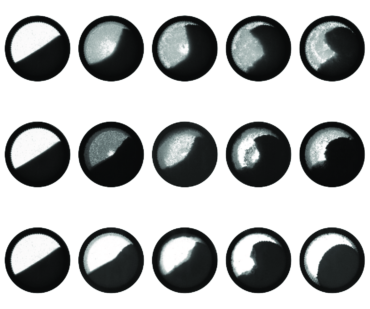
The phenomenology of a cohesive granular medium is much richer than that of cohesionless media and the presence of cohesive interactions between the particles can lead to new types of motion regimes and avalanche dynamics. In fact, even if in this work we focus on a range of Froude numbers that is typical of a rolling motion regime for cohesionless granular media, with the cohesive model material used here there is not a unique motion regime. In the experiments, we observe either intermittent avalanche or continuous flow regimes and the material shows a complex surface morphology that may vary from concave to convex profiles depending on both the particle cohesion and the drum geometry. This variety of behaviours can be observed in figure 3, where characteristic material cross-sections are displayed for different cohesion intensities and drum geometries. The colour indicates the probability of finding the material at various drum coordinates (white indicates a probability $P\lt 10^{-3}$
). For permitting comparison between different geometries we present cases characterized by approximately the same Froude number (
$P\lt 10^{-3}$
). For permitting comparison between different geometries we present cases characterized by approximately the same Froude number ( $\approx 5\times 10^{-3}$
).
$\approx 5\times 10^{-3}$
).
Characteristic drum cross-section for different levels of cohesion and drum geometries ( $d=339\,\unicode{x03BC} \rm m$
,
$d=339\,\unicode{x03BC} \rm m$
, $Fr\approx 5 \times 10^{-3}$
).The drum radius is
$Fr\approx 5 \times 10^{-3}$
).The drum radius is $R=2.5 \, \rm cm$
(top),
$R=2.5 \, \rm cm$
(top), $R=5\, \rm cm$
(middle),
$R=5\, \rm cm$
(middle), $R=9\, \rm cm$
(bottom). The dimensionless width
$R=9\, \rm cm$
(bottom). The dimensionless width $\lambda _W$
associated with each case is reported. The colour scale indicates the probability of finding the material at various drum coordinates (white colour indicates a probability
$\lambda _W$
associated with each case is reported. The colour scale indicates the probability of finding the material at various drum coordinates (white colour indicates a probability $P\lt 10^{-3}$
).
$P\lt 10^{-3}$
).

We globally observe three flow regimes in the drum, depending on the cohesion intensity but also on the drum dimensions:
-
(i) a continuous flow regime in which the surface is planar, the slope is constant in time and the flow occurs continuously in a thin layer close to the surface; this regime occurs for low cohesion and is favoured by long drums. This flow regime is analogous to the one observed for cohesionless particles. However, note that, in the cohesionless case, a continuous flow regime is observed also for the shorter drums;
-
(ii) an intermittent flow regime characterized by several avalanches per rotation, with a concave surface characterized by a double slope. In this regime, which is the most frequently encountered in our experiments, the avalanche is characterized by a mass of nearly triangular section detaching from the top slope and falling to form a new bottom slope;
-
(iii) another continuous flow regime, but characterized by a convex surface, with the granular material ‘rolling’ on the drum body with either some small superficial avalanches or a smooth surface. From figure 3 we can infer that this behaviour occurs preferentially for strong cohesion and in the longer drums.
Qualitatively, in the intermittent avalanche regime, increasing the cohesion yields a steeper average slope with an accentuation of the double-slope character of the material surface profile. However, this is not the case for a highly cohesive material in the longer drums, material for which a change in the motion regime, from an intermittent avalanche to a continuous flow regime, is observed. A tentative explanation for the transition between flow regimes will be discussed in § 4.
Focusing on the drum geometry, we observe that, when comparing cases characterized by approximately the same Froude number, the drum size $R$
has a very mild influence on the shape of the material surface (figure 3). This is quite surprising, given that stresses in the drum should depend on the drum diameter. However, we note small yet significant differences, notably the curvature of the upper part of the material surface. In smaller drums, the surface curvature is higher and the material tends to detach more from the drum body. The drum width
$R$
has a very mild influence on the shape of the material surface (figure 3). This is quite surprising, given that stresses in the drum should depend on the drum diameter. However, we note small yet significant differences, notably the curvature of the upper part of the material surface. In smaller drums, the surface curvature is higher and the material tends to detach more from the drum body. The drum width $W$
has instead a striking effect on the morphology of the material surface profile and its impact is extremely more marked than for the cohesionless case (see figure 3). It should be noted, however, that end walls can exert a considerable influence even in the case of cohesionless materials, as evidenced by their role in determining the S-shaped morphology of the surface profile (Taberlet et al. Reference Taberlet, Richard and Hinch2006). For all the cohesion levels we observed a sharp reduction of the steepness of the surface profile and a progressive attenuation of the double-slope feature when increasing the drum width. In the longer drums, for the lower cohesion levels the surface profile becomes nearly planar, while we observe a convex surface profile for the highest cohesion cases. The lateral walls have therefore a crucial effect on the material dynamics and on the avalanche behaviour, as we are going to see, quantitatively, in the following.
$W$
has instead a striking effect on the morphology of the material surface profile and its impact is extremely more marked than for the cohesionless case (see figure 3). It should be noted, however, that end walls can exert a considerable influence even in the case of cohesionless materials, as evidenced by their role in determining the S-shaped morphology of the surface profile (Taberlet et al. Reference Taberlet, Richard and Hinch2006). For all the cohesion levels we observed a sharp reduction of the steepness of the surface profile and a progressive attenuation of the double-slope feature when increasing the drum width. In the longer drums, for the lower cohesion levels the surface profile becomes nearly planar, while we observe a convex surface profile for the highest cohesion cases. The lateral walls have therefore a crucial effect on the material dynamics and on the avalanche behaviour, as we are going to see, quantitatively, in the following.
3.2. Average surface angle
A simple rather effective description of the surface shape can be given by using an average surface angle. This also allows direct comparison with the cohesionless materials. We recall that, in this work, the surface angle is defined using a ‘centroid’ method, as described in § 2.3.
Average surface angle $\langle \theta \rangle$
versus microscopic Bond number
$\langle \theta \rangle$
versus microscopic Bond number $Bo_m$
for different drum radii
$Bo_m$
for different drum radii $R$
: (a)
$R$
: (a) $W=1\, \rm cm$
, (b)
$W=1\, \rm cm$
, (b) $W=5\, \rm cm$
. The symbol indicates the particle diameter:
$W=5\, \rm cm$
. The symbol indicates the particle diameter: $d=339\,\unicode{x03BC}\rm m$
(
$d=339\,\unicode{x03BC}\rm m$
( $\bullet$
),
$\bullet$
), $d=900\, \unicode{x03BC}\rm m$
(
$d=900\, \unicode{x03BC}\rm m$
( $\blacksquare$
). Data refer to the case
$\blacksquare$
). Data refer to the case $Fr\approx 5 \times 10^{-3}$
. Error bars correspond to the standard deviation.
$Fr\approx 5 \times 10^{-3}$
. Error bars correspond to the standard deviation.

Average surface angle $\langle \theta \rangle$
versus microscopic Bond number
$\langle \theta \rangle$
versus microscopic Bond number $Bo_m$
for different drum widths
$Bo_m$
for different drum widths $W$
: (a)
$W$
: (a) $R=5\, \rm cm$
, (b)
$R=5\, \rm cm$
, (b) $R=2.5\, \rm cm$
. Data refer to the case
$R=2.5\, \rm cm$
. Data refer to the case $d=339\, \unicode{x03BC}\rm m$
,
$d=339\, \unicode{x03BC}\rm m$
, $Fr\approx 5 \times 10^{-3}$
. Error bars correspond to the standard deviation.
$Fr\approx 5 \times 10^{-3}$
. Error bars correspond to the standard deviation.

We display in figures 4 and 5 the evolution of the average surface angle $\langle \theta \rangle$
(
$\langle \theta \rangle$
( $=\ ({1}/{N})\sum ^{N}_i\theta _i$
, where
$=\ ({1}/{N})\sum ^{N}_i\theta _i$
, where $\theta _i$
,
$\theta _i$
, $i=1,\ldots ,N$
is the angle measured in the
$i=1,\ldots ,N$
is the angle measured in the $i$
th frame) as a function of the microscopic Bond number
$i$
th frame) as a function of the microscopic Bond number $Bo_m$
for different values of the drum size
$Bo_m$
for different values of the drum size $R$
and width
$R$
and width $W$
, respectively. Data are compared for experiments at a constant Froude number (
$W$
, respectively. Data are compared for experiments at a constant Froude number ( $Fr\approx 5 \times 10^{-3}$
). The angle
$Fr\approx 5 \times 10^{-3}$
). The angle $\langle \theta \rangle$
is computed by averaging the centroid angle
$\langle \theta \rangle$
is computed by averaging the centroid angle $\theta$
identified in each frame of a single experimental run (5000 images/experiment).
$\theta$
identified in each frame of a single experimental run (5000 images/experiment).
Globally, we observe a systematic increase of the average surface angle $\langle \theta \rangle$
with the particle cohesion, until the appearance of a plateau for the largest values of the microscopic Bond number. The existence of a plateau may have two possible causes: (i) the competing effect of an increase in the interparticle cohesive force and a contemporary decrease in the interparticle frictional force with increasing coating thickness (the coating fills the asperities on the particle surface) and (ii) the existence of a geometric threshold for the vertical orientation of the surface, beyond which the material collapses, irrespective of the magnitude of the cohesive force. It should be noted that this observation applies specifically in the case of the intermittent avalanche regime. In instances where a continuous flow regime with a convex surface is observed, as is the case with highly cohesive materials in long drums, the underlying mechanisms may differ.
$\langle \theta \rangle$
with the particle cohesion, until the appearance of a plateau for the largest values of the microscopic Bond number. The existence of a plateau may have two possible causes: (i) the competing effect of an increase in the interparticle cohesive force and a contemporary decrease in the interparticle frictional force with increasing coating thickness (the coating fills the asperities on the particle surface) and (ii) the existence of a geometric threshold for the vertical orientation of the surface, beyond which the material collapses, irrespective of the magnitude of the cohesive force. It should be noted that this observation applies specifically in the case of the intermittent avalanche regime. In instances where a continuous flow regime with a convex surface is observed, as is the case with highly cohesive materials in long drums, the underlying mechanisms may differ.
Data obtained for two particle sizes are displayed in figure 4. It is evident that, for a given value of $Bo_m$
, larger grains display a larger average angle and thus show a behaviour which is similar to that of increasing cohesion. This is a first element that suggests, as we will discuss later, that the particle-scale Bond number
$Bo_m$
, larger grains display a larger average angle and thus show a behaviour which is similar to that of increasing cohesion. This is a first element that suggests, as we will discuss later, that the particle-scale Bond number $Bo_m$
is not a fully relevant dimensionless number for quantifying the degree of cohesion in the drum. The data in figure 4 indicate also that, for a given Froude number, the morphology of the material surface profile is negligibly influenced by the drum size
$Bo_m$
is not a fully relevant dimensionless number for quantifying the degree of cohesion in the drum. The data in figure 4 indicate also that, for a given Froude number, the morphology of the material surface profile is negligibly influenced by the drum size $R$
. This aligns with the conclusions drawn from visual observation of the material cross-section (§ 3.1). Conversely, the drum width
$R$
. This aligns with the conclusions drawn from visual observation of the material cross-section (§ 3.1). Conversely, the drum width $W$
has a strong effect on the average surface angle, as evidenced in figure 5. We observe a marked reduction in the average surface angle with increasing
$W$
has a strong effect on the average surface angle, as evidenced in figure 5. We observe a marked reduction in the average surface angle with increasing $W$
, a trend that progressively attenuates when transitioning to the case of the longer drums (e.g. comparing case R2.5-W5 with R2.5-W10). It is evident that, in our study, the drum width
$W$
, a trend that progressively attenuates when transitioning to the case of the longer drums (e.g. comparing case R2.5-W5 with R2.5-W10). It is evident that, in our study, the drum width $W$
has a much more pronounced impact on
$W$
has a much more pronounced impact on $\langle \theta \rangle$
in the case of a cohesive material than in the cohesionless case (see also figure 3). Additionally, we observe that the variation of
$\langle \theta \rangle$
in the case of a cohesive material than in the cohesionless case (see also figure 3). Additionally, we observe that the variation of $\langle \theta \rangle$
with
$\langle \theta \rangle$
with $W$
is amplified with increasing the material cohesion.
$W$
is amplified with increasing the material cohesion.
Average surface angle $\langle \theta \rangle$
versus Froude number
$\langle \theta \rangle$
versus Froude number $Fr$
for different cohesion levels: (a)
$Fr$
for different cohesion levels: (a) $Bo_m=8$
, (b)
$Bo_m=8$
, (b) $Bo_m=14$
, (c)
$Bo_m=14$
, (c) $Bo_m=26$
, (d)
$Bo_m=26$
, (d) $Bo_m=44$
. Data refer to the case
$Bo_m=44$
. Data refer to the case $R=5\, \rm cm$
,
$R=5\, \rm cm$
, $d=339\,\unicode{x03BC}\rm m$
. Data for the cohesionless case are displayed in (a) with empty symbols: (
$d=339\,\unicode{x03BC}\rm m$
. Data for the cohesionless case are displayed in (a) with empty symbols: (![]() )
) $W=1\, \rm cm$
, (
$W=1\, \rm cm$
, ( $\triangle$
)
$\triangle$
) $W=5\, \rm cm$
. Error bars correspond to the standard deviation.
$W=5\, \rm cm$
. Error bars correspond to the standard deviation.

Finally, in figure 6 we display the effect of the speed of the drum, via the Froude number, on the average surface angle for different drum widths and cohesion levels. We observe a slight increase of the surface angle with $Fr$
. Furthermore, the impact of the Froude number appears to be linked to both the drum width and the cohesion level. For low cohesion materials, we observe inertial effects on
$Fr$
. Furthermore, the impact of the Froude number appears to be linked to both the drum width and the cohesion level. For low cohesion materials, we observe inertial effects on $\langle \theta \rangle$
in the shorter drums, while they significantly diminish in longer drums. For high cohesive materials the impact of the Froude number on
$\langle \theta \rangle$
in the shorter drums, while they significantly diminish in longer drums. For high cohesive materials the impact of the Froude number on $\langle \theta \rangle$
depends very slightly on the drum width.
$\langle \theta \rangle$
depends very slightly on the drum width.
It should be mentioned that opposite behaviours have been found in the literature: Castellanos et al. Reference Castellanos, Valverde, Pérez, Ramos and Watson(1999) and Neveu et al. (Reference Neveu, Francqui and Lumay2022) observe a decrease of the surface angle with the drum angular speed, while Jarray et al. (Reference Jarray, Magnanimo and Luding2019) and Dong et al. (Reference Dong, Wang, Marks, Chen and Gan2023) observe an increase of the surface angle with the drum speed. This diversity in the dynamic behaviour can be ascribed to the different transition from a solid-like to flow regime (Castellanos et al. Reference Castellanos, Valverde, Pérez, Ramos and Watson1999; Rietema Reference Rietema2012), which strongly depends on the particle size. For fine cohesive powders (diameter below 100 $\,\unicode{x03BC} {\rm m}$
), such as in Castellanos et al. (Reference Castellanos, Valverde, Pérez, Ramos and Watson1999) and Neveu et al. (Reference Neveu, Francqui and Lumay2022), the material may experience fluidization without passing through an inertial flow regime. The region of fluidization exhibits minimal friction with the lateral walls and expands with the drum’s angular velocity, thereby causing a gradual decrease in the surface angle. For coarse granular materials (diameter above 100
$\,\unicode{x03BC} {\rm m}$
), such as in Castellanos et al. (Reference Castellanos, Valverde, Pérez, Ramos and Watson1999) and Neveu et al. (Reference Neveu, Francqui and Lumay2022), the material may experience fluidization without passing through an inertial flow regime. The region of fluidization exhibits minimal friction with the lateral walls and expands with the drum’s angular velocity, thereby causing a gradual decrease in the surface angle. For coarse granular materials (diameter above 100 $\,\unicode{x03BC} {\rm m}$
) in which cohesion arises from liquid capillary bridges instead, such as in Jarray et al. (Reference Jarray, Magnanimo and Luding2019) and Dong et al. (Reference Dong, Wang, Marks, Chen and Gan2023), there is a transition from solid-like behaviour to inertial flow. In this case, the frictional interaction between the granular material and the end walls causes the increase of the surface angle with the drum angular velocity. In the light of the above, we would like to emphasize that it is erroneous to interpret the decrease (increase) of the surface angle with drum speed as a feature of a cohesive (cohesionless) material. This dynamic behaviour seems to stem only from the different transition from a solid-like to flow regime.
$\,\unicode{x03BC} {\rm m}$
) in which cohesion arises from liquid capillary bridges instead, such as in Jarray et al. (Reference Jarray, Magnanimo and Luding2019) and Dong et al. (Reference Dong, Wang, Marks, Chen and Gan2023), there is a transition from solid-like behaviour to inertial flow. In this case, the frictional interaction between the granular material and the end walls causes the increase of the surface angle with the drum angular velocity. In the light of the above, we would like to emphasize that it is erroneous to interpret the decrease (increase) of the surface angle with drum speed as a feature of a cohesive (cohesionless) material. This dynamic behaviour seems to stem only from the different transition from a solid-like to flow regime.
Distribution of the ‘centroid’ surface angle $\theta$
(5000 data for each test). Effect of (a) interparticle cohesion, (b) drum width
$\theta$
(5000 data for each test). Effect of (a) interparticle cohesion, (b) drum width $W$
, (c) drum size
$W$
, (c) drum size $R$
(short drum case), (d) drum size
$R$
(short drum case), (d) drum size $R$
(long drum case). Data refer to the case
$R$
(long drum case). Data refer to the case $d=339\, \unicode{x03BC}\rm m$
,
$d=339\, \unicode{x03BC}\rm m$
, $Fr\approx 5 \times 10^{-3}$
.
$Fr\approx 5 \times 10^{-3}$
.

3.3. Distribution of the surface angle
In order to characterize the distribution of the (centroid) surface angle $\theta$
more in detail, in figure 7 we display the measured probability density
$\theta$
more in detail, in figure 7 we display the measured probability density $P(\theta )$
for the different drum’s geometries and cohesion levels. In figure 7(a) we observe a pronounced influence of the cohesion intensity on the
$P(\theta )$
for the different drum’s geometries and cohesion levels. In figure 7(a) we observe a pronounced influence of the cohesion intensity on the $P(\theta )$
. On the one hand, the distribution is centred around higher values of
$P(\theta )$
. On the one hand, the distribution is centred around higher values of $\theta$
as cohesion increases. On the other hand, the distribution exhibits a greater span with higher cohesion. For relatively high cohesion values, we observe a substantial reduction in its impact on
$\theta$
as cohesion increases. On the other hand, the distribution exhibits a greater span with higher cohesion. For relatively high cohesion values, we observe a substantial reduction in its impact on $P(\theta )$
, and the shape of
$P(\theta )$
, and the shape of $P(\theta )$
remains almost unaltered (cases with
$P(\theta )$
remains almost unaltered (cases with $Bo_m \geq\, 26$
in figure 7
a). This behaviour is coherent with the idea that, for poorly cohesive materials, the avalanche sizes are small and roughly constant, limiting the variation of the surface profile. Conversely, in highly cohesive materials, a broader range of avalanche sizes is possible, leading to increased variability of the surface profile. The above observations also apply to other drum geometries (results not shown here). The only exception is in the limit case of a very long drum and a highly cohesive material, where the motion regime changes from intermittent avalanches to continuous flow. In that case, the span of the distribution gets smaller when approaching the continuous flow regime.
$Bo_m \geq\, 26$
in figure 7
a). This behaviour is coherent with the idea that, for poorly cohesive materials, the avalanche sizes are small and roughly constant, limiting the variation of the surface profile. Conversely, in highly cohesive materials, a broader range of avalanche sizes is possible, leading to increased variability of the surface profile. The above observations also apply to other drum geometries (results not shown here). The only exception is in the limit case of a very long drum and a highly cohesive material, where the motion regime changes from intermittent avalanches to continuous flow. In that case, the span of the distribution gets smaller when approaching the continuous flow regime.
In figure 7(b–d), we display the effect of the drum geometry on the probability density of the centroid angle $\theta$
. Beginning with an analysis of the effect of the drum width (figure 7
b), we observe, as was evident from the previous section, that
$\theta$
. Beginning with an analysis of the effect of the drum width (figure 7
b), we observe, as was evident from the previous section, that $P(\theta )$
is centred on higher angles for shorter drums. We also observe that the distribution is wider for smaller values of
$P(\theta )$
is centred on higher angles for shorter drums. We also observe that the distribution is wider for smaller values of $W$
, suggesting a broader range of avalanche sizes in shorter drums. This behaviour persists across various cohesion levels. We hypothesize that such behaviour is associated with the interaction between the material and the lateral walls. In short drums, the interaction of the material with the walls is strong. This interaction has a non-trivial effect on the shape of the material surface and may have an interplay with interparticle cohesion in the formation of avalanches, stabilizing the material and thus broadening their possible size. In long drums instead, the interaction with the walls is weak, leading to a scenario where material stability is predominantly governed by material properties and a ‘characteristic’ size of avalanches emerges more clearly.
$W$
, suggesting a broader range of avalanche sizes in shorter drums. This behaviour persists across various cohesion levels. We hypothesize that such behaviour is associated with the interaction between the material and the lateral walls. In short drums, the interaction of the material with the walls is strong. This interaction has a non-trivial effect on the shape of the material surface and may have an interplay with interparticle cohesion in the formation of avalanches, stabilizing the material and thus broadening their possible size. In long drums instead, the interaction with the walls is weak, leading to a scenario where material stability is predominantly governed by material properties and a ‘characteristic’ size of avalanches emerges more clearly.
Distribution of the avalanche size $\tilde {S}_a$
. Effect of (a) interparticle cohesion, (b) drum width
$\tilde {S}_a$
. Effect of (a) interparticle cohesion, (b) drum width $W$
, (c) drum size
$W$
, (c) drum size $R$
(short drum case), (d) drum size
$R$
(short drum case), (d) drum size $R$
(long drum case). The number in round brackets shows the number of avalanches detected in each experiment. Data refer to the case
$R$
(long drum case). The number in round brackets shows the number of avalanches detected in each experiment. Data refer to the case $d=339\,\unicode{x03BC}\rm m$
,
$d=339\,\unicode{x03BC}\rm m$
, $Fr\approx 5 \times 10^{-3}$
. (e) Average avalanche size
$Fr\approx 5 \times 10^{-3}$
. (e) Average avalanche size $\langle \tilde {S}_a \rangle$
versus the standard deviation of the centroid angle
$\langle \tilde {S}_a \rangle$
versus the standard deviation of the centroid angle $\sigma (\theta )$
. Only experiments for which the average avalanche size is greater than the systematic uncertainty are displayed. The avalanche size is normalized with respect to the theoretical material cross-section. The red bar in each panel corresponds to the systematic uncertainty on the avalanche size as defined in § 2.3.
$\sigma (\theta )$
. Only experiments for which the average avalanche size is greater than the systematic uncertainty are displayed. The avalanche size is normalized with respect to the theoretical material cross-section. The red bar in each panel corresponds to the systematic uncertainty on the avalanche size as defined in § 2.3.

The drum size $R$
has a very mild effect on the distribution of
$R$
has a very mild effect on the distribution of $\theta$
, with only the span of the distribution tending to increase when decreasing the drum size
$\theta$
, with only the span of the distribution tending to increase when decreasing the drum size $R$
. This can be related to an increase of the relative size of the avalanche with respect to the drum size in smaller drums. To substantiate the assumptions made regarding the avalanche size in interpreting the observed distribution of surface angles, we devote § 3.4 to a detailed discussion on the avalanche size distribution and its dependence on cohesion and the drum geometry.
$R$
. This can be related to an increase of the relative size of the avalanche with respect to the drum size in smaller drums. To substantiate the assumptions made regarding the avalanche size in interpreting the observed distribution of surface angles, we devote § 3.4 to a detailed discussion on the avalanche size distribution and its dependence on cohesion and the drum geometry.
3.4. Distribution of avalanche sizes
In this section, we focus on the statistical distribution of the avalanche size computed as described in § 2.3. We display in figure (8
a–d) the probability density of the avalanche size for different cohesion levels and drum geometries. Note that we display the avalanche size normalized with respect to the theoretical material cross-section ( $\tilde {S}_a=S_a/S_g,$
with
$\tilde {S}_a=S_a/S_g,$
with $S_g=\pi R^2/2$
).
$S_g=\pi R^2/2$
).
The distribution in figure 8(a) clearly shows that cohesion has a crucial impact on the typical avalanche size, with the average size increasing with interparticle cohesion. For low cohesion we observe a single peak in the distribution, which suggests that the system has a characteristic avalanche size. For high interparticle cohesion, instead, we observe a very broad distribution which is symptomatic of the coexistence of small and large avalanches in the system. This is associated with the fact that, in our system, the formation of an avalanche is strictly dependent on the surface morphology created by the previous avalanche, and for a highly cohesive material, this surface may be rather irregular and characterized by strong fluctuations. A large avalanche event determines a strong perturbation of the material surface that subsequently exhibits a much lower slope angle and may become quite irregular. This yields to two possible future scenarios: (i) a phase of rigid rotation of the material with the drum body (the previous avalanche has formed a smooth surface), (ii) a succession of small avalanches that smooth out the material surface (the preceding avalanche has formed an irregular surface) before the potential formation of a new large avalanche event. This behaviour is consistent with what has been observed in wet granular systems (Brewster et al. Reference Brewster, Grest and Levine2009) and fine cohesive powders (Quintanilla et al. Reference Quintanilla, Valverde, Castellanos and Viturro2001). There is also the intriguing possibility that the broad tail of the distribution could yield a non-zero probability of complete clogging, which would be visible for sufficiently long times. This is an interesting aspect which we wish to study in the future.
The effect of the drum width $W$
on the avalanche size distribution
$W$
on the avalanche size distribution $P{(\tilde {S}_a)}$
is shown in figure 8(b). We observe that, for shorter drums, not only is the avalanche size systematically larger, but also the potential range of the typical avalanche sizes becomes wider (i.e. span of the distribution increases for lower
$P{(\tilde {S}_a)}$
is shown in figure 8(b). We observe that, for shorter drums, not only is the avalanche size systematically larger, but also the potential range of the typical avalanche sizes becomes wider (i.e. span of the distribution increases for lower $W$
). The interaction with the lateral walls stabilizes the material, allowing larger avalanches to form in shorter drums. As discussed above, larger avalanche events are associated with stronger fluctuations of the material surface, which in turns cause a higher variability of the potential size of the future avalanches. In this context, reducing the drum width has an effect which is similar to that of increasing cohesion. The effect of the drum size
$W$
). The interaction with the lateral walls stabilizes the material, allowing larger avalanches to form in shorter drums. As discussed above, larger avalanche events are associated with stronger fluctuations of the material surface, which in turns cause a higher variability of the potential size of the future avalanches. In this context, reducing the drum width has an effect which is similar to that of increasing cohesion. The effect of the drum size $R$
on the avalanche size distribution
$R$
on the avalanche size distribution $P{(\tilde {S}_a)}$
is shown in figure 8(c–d). We note that the typical avalanche size is larger and has greater variability in size in smaller drums. We can reasonably assume that the typical avalanche size is strongly correlated with the cohesion intensity. Consequently, it is not surprising to observe larger avalanches – with respect to the system size – in smaller drums. The broader spectrum of avalanche sizes can be explained by the fact that larger avalanche events lead to stronger fluctuations of the material surface. This picture, which relates avalanche size and fluctuations of the material surface, is also supported by the strong correlation between the standard deviation of the average surface angle
$P{(\tilde {S}_a)}$
is shown in figure 8(c–d). We note that the typical avalanche size is larger and has greater variability in size in smaller drums. We can reasonably assume that the typical avalanche size is strongly correlated with the cohesion intensity. Consequently, it is not surprising to observe larger avalanches – with respect to the system size – in smaller drums. The broader spectrum of avalanche sizes can be explained by the fact that larger avalanche events lead to stronger fluctuations of the material surface. This picture, which relates avalanche size and fluctuations of the material surface, is also supported by the strong correlation between the standard deviation of the average surface angle $\sigma (\theta )$
and the average avalanche size observed in our experiments (figure 8
e).
$\sigma (\theta )$
and the average avalanche size observed in our experiments (figure 8
e).
In light of the aforementioned discussion, it appears that reducing the system size – along either the axial or radial direction – results in a behaviour which is consistent with an increment of the particle cohesion. This suggests that there is a strong interplay between the material (and cohesion intensity in particular) and the drum geometry, that in some cases may lead to the emergence of size effects. This aspect will be further discussed in § 4.
4. Discussion
In the results presented in the previous section, we observed that several parameters affect, qualitatively and quantitatively, the flow behaviour of a cohesive granular material in a rotating drum. The most important parameters are clearly the intensity of the cohesion, which we estimated with the microscopic Bond number $Bo_m$
, and the width of the drum
$Bo_m$
, and the width of the drum $W$
. The drum radius
$W$
. The drum radius $R$
, while having a negligible effect on the average surface angle, exerts a substantial influence on the avalanche dynamics. This underscores that the surface morphology as well as the material dynamics are not simply a function of the material properties but are also closely linked to the geometry of the drum.
$R$
, while having a negligible effect on the average surface angle, exerts a substantial influence on the avalanche dynamics. This underscores that the surface morphology as well as the material dynamics are not simply a function of the material properties but are also closely linked to the geometry of the drum.
To explain the observed variation in the shape of the free surface with the drum width $W$
, we assume that this variation may be attributed to the interplay between the material and the end walls. This aspect is discussed further below. For cohesionless particles it is well known that wall effects may have a strong impact on the stability of a granular pile. This is associated with the formation of particle arches that can transmit a part of the weight to the walls. In these systems, the pile angle decreases with an increasing wall gap towards constant values and the characteristic length of wall effects has been shown to be proportional to the particle diameter (Grasselli & Herrmann Reference Grasselli and Herrmann1997; Boltenhagen Reference Boltenhagen1999; du Pont et al. Reference du Pont, Gondret, Perrin and Rabaud2003). It is therefore natural for us to attempt to associate the observed variation of the surface angle in our system with the width of the drum with the same physical mechanism. In this perspective, we define a dimensionless width
$W$
, we assume that this variation may be attributed to the interplay between the material and the end walls. This aspect is discussed further below. For cohesionless particles it is well known that wall effects may have a strong impact on the stability of a granular pile. This is associated with the formation of particle arches that can transmit a part of the weight to the walls. In these systems, the pile angle decreases with an increasing wall gap towards constant values and the characteristic length of wall effects has been shown to be proportional to the particle diameter (Grasselli & Herrmann Reference Grasselli and Herrmann1997; Boltenhagen Reference Boltenhagen1999; du Pont et al. Reference du Pont, Gondret, Perrin and Rabaud2003). It is therefore natural for us to attempt to associate the observed variation of the surface angle in our system with the width of the drum with the same physical mechanism. In this perspective, we define a dimensionless width $\lambda _W$
:
$\lambda _W$
:
 \begin{equation} \lambda _W=\dfrac {W}{\mbox {max}(d\it ,Bo_md)}=\dfrac {W}{\mbox {max}({d},l_c)}, \end{equation}
where $l_c$
is a cohesive length, i.e. the length for which gravitational effects are balanced by cohesive effects (
$l_c$
is a cohesive length, i.e. the length for which gravitational effects are balanced by cohesive effects ( $l_c=Bo_md$
). In figure 9(a) we display the average surface angle as a function of the dimensionless width
$l_c=Bo_md$
). In figure 9(a) we display the average surface angle as a function of the dimensionless width $\lambda _W$
for different cohesion intensities, drum geometries and particle diameters, at a constant Froude number. The data scale with
$\lambda _W$
for different cohesion intensities, drum geometries and particle diameters, at a constant Froude number. The data scale with $\lambda _W$
, showing that it is a relevant length scale in our system. Similarly to what has been observed for cohesionless particles (Grasselli & Herrmann Reference Grasselli and Herrmann1997; Boltenhagen Reference Boltenhagen1999; du Pont et al. Reference du Pont, Gondret, Perrin and Rabaud2003), the behaviour of the surface angle can be described by an exponential law of the form
$\lambda _W$
, showing that it is a relevant length scale in our system. Similarly to what has been observed for cohesionless particles (Grasselli & Herrmann Reference Grasselli and Herrmann1997; Boltenhagen Reference Boltenhagen1999; du Pont et al. Reference du Pont, Gondret, Perrin and Rabaud2003), the behaviour of the surface angle can be described by an exponential law of the form
 \begin{equation} \theta =\theta _{\infty }\left [1+\alpha \exp (-\lambda _W/\lambda _W^*)\right ], \end{equation}
with three fitting parameters: $\theta _{\infty }$
is the surface angle when
$\theta _{\infty }$
is the surface angle when $\lambda _W$
tends towards infinity,
$\lambda _W$
tends towards infinity, $\lambda _W^*$
may be seen as a characteristic dimensionless length over which most of the wall effects vanish and
$\lambda _W^*$
may be seen as a characteristic dimensionless length over which most of the wall effects vanish and $\alpha$
is a numerical coefficient. In the inset of figure 9(a), we report the angle of the top slope
$\alpha$
is a numerical coefficient. In the inset of figure 9(a), we report the angle of the top slope $\theta _{top}$
as a function of the dimensionless width
$\theta _{top}$
as a function of the dimensionless width $\lambda _W$
. Only cases for which a clear double-slope profile was clearly identifiable are considered (cases with
$\lambda _W$
. Only cases for which a clear double-slope profile was clearly identifiable are considered (cases with $W\lt 5\,\rm cm$
). We observe that
$W\lt 5\,\rm cm$
). We observe that $\theta _{top}$
seems to scale well with the dimensionless width
$\theta _{top}$
seems to scale well with the dimensionless width $\lambda _W$
and data are well fitted by the exponential law of (4.2). This provides a further confirmation that the ratio between the drum width and the cohesive length is a relevant quantity in the studied system. Finally, when considering data for all Froude numbers (figure 9
b), they display some dispersion but still the scaling is clear (the fit of the experimental data gives
$\lambda _W$
and data are well fitted by the exponential law of (4.2). This provides a further confirmation that the ratio between the drum width and the cohesive length is a relevant quantity in the studied system. Finally, when considering data for all Froude numbers (figure 9
b), they display some dispersion but still the scaling is clear (the fit of the experimental data gives $\theta _{\infty }=38^{\circ }$
,
$\theta _{\infty }=38^{\circ }$
, $\lambda _W^*= 4.2$
,
$\lambda _W^*= 4.2$
, $\alpha =1.02$
). However, the variation range of the Froude number was limited, and we expect a dependence on
$\alpha =1.02$
). However, the variation range of the Froude number was limited, and we expect a dependence on $Fr$
over a broader range than that considered in the present study.
$Fr$
over a broader range than that considered in the present study.
Average surface angle $\langle \theta \rangle$
versus the dimensionless width
$\langle \theta \rangle$
versus the dimensionless width $\lambda _W$
. Data in (a) refer to the case
$\lambda _W$
. Data in (a) refer to the case $Fr\approx 5 \times 10^{-3}$
. The inset in (a) shows the average top angle
$Fr\approx 5 \times 10^{-3}$
. The inset in (a) shows the average top angle $\langle \theta _{top}\rangle$
versus the dimensionless width
$\langle \theta _{top}\rangle$
versus the dimensionless width $\lambda _W$
(data are fitted with (4.2),
$\lambda _W$
(data are fitted with (4.2), $\theta _{\infty }=47^{\circ }$
,
$\theta _{\infty }=47^{\circ }$
, $\lambda _W^*=3.7$
,
$\lambda _W^*=3.7$
, $\alpha =1.6$
). In the inset in (b) the
$\alpha =1.6$
). In the inset in (b) the $x$
-axis is in logarithmic scale and data obtained for cohesionless particles are reported (
$x$
-axis is in logarithmic scale and data obtained for cohesionless particles are reported ( $\blacktriangleright$
). Error bars correspond to the standard deviation.
$\blacktriangleright$
). Error bars correspond to the standard deviation.

This empirical result demonstrates the enormous impact of the lateral walls on the behaviour of cohesive granular materials. Differently from the case of cohesionless particles, for which the decay length of the walls effects is of the order of a few bead diameters, in cohesive granular materials the cohesive length $l_c$
is the relevant length, which can be much larger than the bead diameter (
$l_c$
is the relevant length, which can be much larger than the bead diameter ( $\propto Bo_m d$
) and may become comparable to the drum width. This point is particularly crucial if one thinks that many analyses, even in powder testing, are made with drums of relatively short width (Pachón-Morales et al. Reference Pachón-Morales, Colin, Casalinho, Perré and Puel2020; Neveu et al. Reference Neveu, Francqui and Lumay2022; Jabaud et al. Reference Jabaud, Artoni, Tobie, le Menn and Richard2024), in which the effect of lateral walls is stronger.
$\propto Bo_m d$
) and may become comparable to the drum width. This point is particularly crucial if one thinks that many analyses, even in powder testing, are made with drums of relatively short width (Pachón-Morales et al. Reference Pachón-Morales, Colin, Casalinho, Perré and Puel2020; Neveu et al. Reference Neveu, Francqui and Lumay2022; Jabaud et al. Reference Jabaud, Artoni, Tobie, le Menn and Richard2024), in which the effect of lateral walls is stronger.
This interpretation based on the dimensionless width $\lambda _W$
allows consistent distinction between short drums (
$\lambda _W$
allows consistent distinction between short drums ( $W \sim l_c$
), in which end wall effects are significant, and long drums (
$W \sim l_c$
), in which end wall effects are significant, and long drums ( $W \gg l_c$
), in which the impact of the end walls on the material dynamics is negligible. Note that the concept of short/long is not purely geometric, but associates the drum geometry with the material properties. This is not only fundamental for the transfer of results from the laboratory to the real life and vice versa (scale-up and scale-down), but is also useful for numerical, discrete element, simulations, in which researchers often try to mimic the behaviour of fine cohesive particles with coarser grains by tuning attractive force parameters. In addition to the experimental results, a simple theoretical model inspired by the one used to explain superstable heaps in Taberlet et al. (Reference Taberlet, Richard, Valance, Losert, Pasini, Jenkins and Delannay2003), is presented in Appendix A. The model predicts that, for a cohesive granular material, the surface inclination at the onset of the flow depends on the quantity
$W \gg l_c$
), in which the impact of the end walls on the material dynamics is negligible. Note that the concept of short/long is not purely geometric, but associates the drum geometry with the material properties. This is not only fundamental for the transfer of results from the laboratory to the real life and vice versa (scale-up and scale-down), but is also useful for numerical, discrete element, simulations, in which researchers often try to mimic the behaviour of fine cohesive particles with coarser grains by tuning attractive force parameters. In addition to the experimental results, a simple theoretical model inspired by the one used to explain superstable heaps in Taberlet et al. (Reference Taberlet, Richard, Valance, Losert, Pasini, Jenkins and Delannay2003), is presented in Appendix A. The model predicts that, for a cohesive granular material, the surface inclination at the onset of the flow depends on the quantity $Bo_md/W$
, thereby supporting our phenomenological scaling.
$Bo_md/W$
, thereby supporting our phenomenological scaling.
Although the drum size $R$
does not have a relevant effect on the average surface angle (see § 3.2 and the scaling in figure 9), we have shown in §§ 3.3 and 3.4 that it clearly does have an impact on the dynamics of the material and the statistical properties of the avalanche size. This suggests that the average surface angle is probably a too much lumped parameter if one would like to describe the full dynamics of the material in the drum. The average avalanche size, for instance, appears to be – somewhat obviously – strongly correlated to the span of the centroid angle distribution (figure 8
e). This indicates that the standard deviation of the centroid angle distribution, that we used for example in a recent work (Jabaud et al. Reference Jabaud, Artoni, Tobie, le Menn and Richard2024), might be a good additional descriptor of the material dynamics. Unfortunately, we did not succeed in finding a proper scaling for that quantity. The mild impact on the surface morphology observed when changing the drum radius
$R$
does not have a relevant effect on the average surface angle (see § 3.2 and the scaling in figure 9), we have shown in §§ 3.3 and 3.4 that it clearly does have an impact on the dynamics of the material and the statistical properties of the avalanche size. This suggests that the average surface angle is probably a too much lumped parameter if one would like to describe the full dynamics of the material in the drum. The average avalanche size, for instance, appears to be – somewhat obviously – strongly correlated to the span of the centroid angle distribution (figure 8
e). This indicates that the standard deviation of the centroid angle distribution, that we used for example in a recent work (Jabaud et al. Reference Jabaud, Artoni, Tobie, le Menn and Richard2024), might be a good additional descriptor of the material dynamics. Unfortunately, we did not succeed in finding a proper scaling for that quantity. The mild impact on the surface morphology observed when changing the drum radius $R$
indicates that, in the studied systems, end walls effects are stronger than possible effects related to the size of the drum along the radial direction. However, we can suppose that, in long drums, for which end walls effects are negligible, we might start to observe effects related to the size of the system when the drum size is comparable to the cohesive length. To test this hypothesis, in analogy to what was done when discussing the effect of the drum width, we introduce the dimensionless radius
$R$
indicates that, in the studied systems, end walls effects are stronger than possible effects related to the size of the drum along the radial direction. However, we can suppose that, in long drums, for which end walls effects are negligible, we might start to observe effects related to the size of the system when the drum size is comparable to the cohesive length. To test this hypothesis, in analogy to what was done when discussing the effect of the drum width, we introduce the dimensionless radius $\lambda _R$
:
$\lambda _R$
:
 \begin{equation} \lambda _R=\dfrac {R}{\mbox {max}(d\it ,Bo_md)}=\dfrac {R}{\mbox {max}(d\it ,l_c)}. \end{equation}
In our experiments $\lambda _R$
is the lowest for the cases with
$\lambda _R$
is the lowest for the cases with $R=2.5 \,\rm cm$
,
$R=2.5 \,\rm cm$
, $Bo_m=44$
,
$Bo_m=44$
, $d=339\, \unicode{x03BC} \rm m $
(
$d=339\, \unicode{x03BC} \rm m $
( $\lambda _R=1.7$
). In these cases, we observe a remarkable curvature of the surface of the material, especially in long drums, with the whole material surface becoming convex in the extreme case
$\lambda _R=1.7$
). In these cases, we observe a remarkable curvature of the surface of the material, especially in long drums, with the whole material surface becoming convex in the extreme case $W=10\, \rm cm$
for which we can assume that end walls’ effects are completely negligible (see figure 3). This behaviour can be reasonably seen as a potential symptom of size effects in the radial direction. Furthermore, a gentle yet significant impact on the curvature of the material surface is also observed in the short drum case when changing the drum radius (compare cases with
$W=10\, \rm cm$
for which we can assume that end walls’ effects are completely negligible (see figure 3). This behaviour can be reasonably seen as a potential symptom of size effects in the radial direction. Furthermore, a gentle yet significant impact on the curvature of the material surface is also observed in the short drum case when changing the drum radius (compare cases with $Bo_m=44$
in figure 3). This supports the hypothesis that
$Bo_m=44$
in figure 3). This supports the hypothesis that $\lambda _R$
may be another relevant length scale for accounting for size effects in our system. It seems therefore possible to distinguish, analogously to the case of short/long drums, between small drums (
$\lambda _R$
may be another relevant length scale for accounting for size effects in our system. It seems therefore possible to distinguish, analogously to the case of short/long drums, between small drums ( $R \sim l_c$
), in which the interaction with the drum body causes a strong curvature of the surface of the granular material, and large drums (
$R \sim l_c$
), in which the interaction with the drum body causes a strong curvature of the surface of the granular material, and large drums ( $R \gg l_c$
), in which material surface is not affected by the geometry of the drum.
$R \gg l_c$
), in which material surface is not affected by the geometry of the drum.
To conclude our analysis, we attempt to propose an interpretation for the three different flow regimes and the associated transitions observed in the experiments:
-
(i) planar continuous flow – the cohesive length is much lower than the drum dimensions (i.e. $l_c \ll W, R$
) and size effects are negligible. In this situation the material behaves similarly to a cohesionless material;
$l_c \ll W, R$
) and size effects are negligible. In this situation the material behaves similarly to a cohesionless material; -
(ii) intermittent avalanche flow – the cohesive length starts to be comparable to the drum width (i.e.
$l_c \sim W$
) and size effects in the axial direction start to emerge. This yields a concave free surface and an intermittent flow regime; -
(iii) convex continuous flow – the cohesive length starts to be comparable to the drum radius while walls effects are negligible (i.e.
$l_c \sim R$
and
$l_c \ll W$
). In this case size effects in the radial direction clearly emerge. The upper part of the material surface start to be strongly curved and for relatively low values of
$\lambda _R$
the whole surface becomes convex with the material rolling on the drum body.


5. Conclusions
In this paper we studied experimentally the dynamics of a cohesive granular material in a rotating drum, changing in a systematic way the cohesion intensity and the drum geometry.
We showed that, for a cohesive granular material, the flow phenomenology is much richer than that typical of a cohesionless one. We observed three main flow regimes: (i) a continuous flow regime with a planar surface, (ii) an intermittent flow regime with several avalanches per rotation with a concave surface, (iii) a continuous flow regime with a convex surface. We have associated the transition between flow regimes with size effects, which are controlled by the ratio of the axial and radial dimensions of the drum and the cohesive length, i.e. the length at which gravity balances the cohesive stress.
We presented an experimental evidence of the substantial impact of the lateral walls on the morphology of the free surface of the material in the rotating drum geometry. We provided a physical interpretation of the role of wall effects in terms of a dimensionless width $\lambda _W$
, which is defined as the ratio between the drum width and the cohesive length. We showed that the average surface angle scales well with
$\lambda _W$
, which is defined as the ratio between the drum width and the cohesive length. We showed that the average surface angle scales well with $\lambda _W$
, and that this dimensionless width may serve as a criterion to differentiate between short and long drums, where end wall effects are either significant or negligible, respectively. It should be noted that particle–wall friction may influence the relevance of the lateral wall, with a reduction (increase) in particle–wall friction leading to a mitigation (intensification) of end wall effects, as indicated by the theoretical model in Appendix A and similarly to what occurs in the cohesionless case (Taberlet et al. Reference Taberlet, Richard and Hinch2006). However, except in the limiting case of frictionless contact, we believe that changing the particle–wall friction does not alter the underlying physics of the phenomenon, which remains governed by the dimensionless width
$\lambda _W$
, and that this dimensionless width may serve as a criterion to differentiate between short and long drums, where end wall effects are either significant or negligible, respectively. It should be noted that particle–wall friction may influence the relevance of the lateral wall, with a reduction (increase) in particle–wall friction leading to a mitigation (intensification) of end wall effects, as indicated by the theoretical model in Appendix A and similarly to what occurs in the cohesionless case (Taberlet et al. Reference Taberlet, Richard and Hinch2006). However, except in the limiting case of frictionless contact, we believe that changing the particle–wall friction does not alter the underlying physics of the phenomenon, which remains governed by the dimensionless width $\lambda _W$
.
$\lambda _W$
.
Finally, we found that the avalanche size distribution is strongly dependent not only on the cohesion intensity but also on the drum geometry. Higher cohesion leads to the formation of large avalanches which are interspersed with subsequent events of small avalanches. The alternation of large and small avalanche events is also observed when decreasing either the drum width or the drum radius, which has therefore an effect similar to increasing cohesion.
The results presented in this work push us to develop further analyses to find scaling laws for the full distribution of the surface angle, which should be valid for different drum dimensions and material properties. In order to study this point more in detail, it seems fundamental to refine the experimental analysis by extracting more local measurements of the surface profile, but also to perform discrete element simulations of the rotating drum flow to tackle the mechanical origin of the avalanche behaviour, particularly quantifying subjacent aspects such as the build-up of the porosity in the sample and its interrelation with the avalanche dynamics. Moreover, numerical simulations will permit us to test our hypotheses on flow regime transitions.
In this study, we adopted a cohesive model material in which the behaviour of the cohesive force is reminiscent of that typical of liquid capillary bridges. It should be noted that our findings might not be directly extendable to granular systems in which cohesion has a different origin. Nevertheless, we believe that the crucial role of the boundary effects and the fact that the cohesive length appears to be the relevant scale for understanding their impact on material behaviour are results of general validity.
Acknowledgements
Authors are grateful to J.-M. Paul and J. Le Mouel for their technical support. The authors wish also to thank M. Nicolas for fruitful and inspiring discussions. The authors are grateful to the anonymous reviewers for their valuable comments, which have contributed to improving this article.
Funding
The authors acknowledge financial support from ANR (grant no. ANR-20-CE08-592 0028 MoNoCoCo) and from Region Pays de la Loire (project GRIM).
Declaration of interests
The authors report no conflict of interest.
Appendix A. Theoretical model of a laterally confined cohesive granular heap
In the paper we have shown that, for a cohesive material, the average surface angle scales with the dimensionless width $\lambda _W=W/\max ({d},l_c)$
, where
$\lambda _W=W/\max ({d},l_c)$
, where $W$
is the gap between the sidewalls, i.e. the drum width in our system, and
$W$
is the gap between the sidewalls, i.e. the drum width in our system, and $l_c$
is equal to
$l_c$
is equal to $Bo_m d$
, with
$Bo_m d$
, with $Bo_m$
the microscopic Bond number (2.2) and
$Bo_m$
the microscopic Bond number (2.2) and $d$
the particle diameter. In this appendix, we will show that this scaling can be explained by a simple model similar to that used to explain the presence of superstable heaps in confined granular flows (Taberlet et al. Reference Taberlet, Richard, Valance, Losert, Pasini, Jenkins and Delannay2003).
$d$
the particle diameter. In this appendix, we will show that this scaling can be explained by a simple model similar to that used to explain the presence of superstable heaps in confined granular flows (Taberlet et al. Reference Taberlet, Richard, Valance, Losert, Pasini, Jenkins and Delannay2003).
Let us consider a slab of granular material (mass density $\rho _g$
), parallel to the free surface, located between the surface and a depth
$\rho _g$
), parallel to the free surface, located between the surface and a depth $h$
(see figure 10), flowing uniformly along the
$h$
(see figure 10), flowing uniformly along the $x$
-direction on a stable heap beneath. The forces parallel to the
$x$
-direction on a stable heap beneath. The forces parallel to the $x$
-axis that are exerted on that slab are (i) the corresponding weight component
$x$
-axis that are exerted on that slab are (i) the corresponding weight component $F_g$
, (ii) the friction of the lateral walls
$F_g$
, (ii) the friction of the lateral walls $F_w$
, (iii) the friction at the base of the slab
$F_w$
, (iii) the friction at the base of the slab $F_b$
and (iv) the cohesion force at the base of the slab
$F_b$
and (iv) the cohesion force at the base of the slab $F_c$
(see figure 10
b). Following Taberlet et al. (Reference Taberlet, Richard, Valance, Losert, Pasini, Jenkins and Delannay2003) we assume a constant volume fraction and that the friction forces follow the Coulomb law (the friction of the wall and of the granular bed are respectively characterized by the friction coefficients
$F_c$
(see figure 10
b). Following Taberlet et al. (Reference Taberlet, Richard, Valance, Losert, Pasini, Jenkins and Delannay2003) we assume a constant volume fraction and that the friction forces follow the Coulomb law (the friction of the wall and of the granular bed are respectively characterized by the friction coefficients $\mu _W$
and
$\mu _W$
and $\mu _B$
). The sum of the forces parallel to the
$\mu _B$
). The sum of the forces parallel to the $x$
-axis normalized by the
$x$
-axis normalized by the $z$
-component of the weight gives
$z$
-component of the weight gives
 \begin{equation} \tan \theta = \mu _B + \mu _W\frac {h}{W} + \frac {\lambda _c}{h \cos \theta }, \end{equation}
where $\lambda _c$
has the dimension of a length and is defined as
$\lambda _c$
has the dimension of a length and is defined as $\lambda _c = \tau _c/\rho g$
,
$\lambda _c = \tau _c/\rho g$
, $\tau _c$
being the cohesive stress. For a given inclination
$\tau _c$
being the cohesive stress. For a given inclination $\theta$
there exists a solution for
$\theta$
there exists a solution for $h$
only if
$h$
only if
 \begin{equation} \tan \theta \geq \mu _B+\sqrt {\mu _W\frac {\lambda _c }{W}}\left (\sqrt {\cos \theta } + {1}/{\sqrt {\cos \theta }} \right ), \end{equation}
which corresponds to the minimum of $f(h)=\mu _B + \mu _W {h}/{W} + {\lambda _c}/{h \cos \theta }.$
In the range of angles considered in this work, since
$f(h)=\mu _B + \mu _W {h}/{W} + {\lambda _c}/{h \cos \theta }.$
In the range of angles considered in this work, since $\tan \theta$
varies faster than
$\tan \theta$
varies faster than $\psi (\theta ) = \sqrt {\cos \theta } + {1}/{\sqrt {\cos \theta }}$
, we can neglect the variation of the quantity
$\psi (\theta ) = \sqrt {\cos \theta } + {1}/{\sqrt {\cos \theta }}$
, we can neglect the variation of the quantity $\psi (\theta )$
to simplify the expression of
$\psi (\theta )$
to simplify the expression of $f(h)$
. In this simplified framework, for a given
$f(h)$
. In this simplified framework, for a given $\theta$
, the condition on the force balances is
$\theta$
, the condition on the force balances is
 \begin{equation} \tan \theta \geq \mu _B+\kappa \sqrt {\mu _W\frac {\lambda _c }{W}}, \end{equation}
where $\kappa$
is a constant corresponding to an average value of
$\kappa$
is a constant corresponding to an average value of $\psi (\theta )= (\sqrt {\cos \theta } + {1}/{\sqrt {\cos \theta }} )$
; this can reasonably be approximated as 2, at least for angles up to
$\psi (\theta )= (\sqrt {\cos \theta } + {1}/{\sqrt {\cos \theta }} )$
; this can reasonably be approximated as 2, at least for angles up to $70^\circ$
(
$70^\circ$
( $\psi (70^\circ )\approx 2.3$
).
$\psi (70^\circ )\approx 2.3$
).
(a) Three-dimensional sketch of the geometry considered in the theoretical model. (b) Sketch of the forces considered in the theoretical model. For a slab of length $dL$
, the forces are
$dL$
, the forces are $F_g=\rho g h W {d}L \sin \theta$
,
$F_g=\rho g h W {d}L \sin \theta$
, $F_b=\mu _B \rho g h W {d}L \cos \theta$
,
$F_b=\mu _B \rho g h W {d}L \cos \theta$
, $F_c=\tau _c W {d}L$
,
$F_c=\tau _c W {d}L$
, $F_w=\mu _W \rho g h^2 {d}L \cos \theta$
.
$F_w=\mu _W \rho g h^2 {d}L \cos \theta$
.

Tangent of the average surface angle $\langle \theta \rangle$
versus
$\langle \theta \rangle$
versus $\sqrt {{Bo_m d}/{W}}$
. Consistent with (A6), data are fitted by an affine function of
$\sqrt {{Bo_m d}/{W}}$
. Consistent with (A6), data are fitted by an affine function of $\sqrt {{Bo_m d}/{W}}$
(dashed line).
$\sqrt {{Bo_m d}/{W}}$
(dashed line).

Following Gans et al. (Reference Gans, Pouliquen and Nicolas2020), the cohesive stress $\tau _c$
can be expressed as
$\tau _c$
can be expressed as
 \begin{equation} \tau _c= \frac {3 \mu _B \phi Z F_c}{2 \pi d^2} ,\end{equation}
where $Z$
is the coordination number (average number of contacts per particle). The relation (A4) associated with (2.1) gives
$Z$
is the coordination number (average number of contacts per particle). The relation (A4) associated with (2.1) gives
 \begin{equation} \lambda _c=\frac {\mu _B \phi Z Bo_m d}{4} .\end{equation}
Finally, by plugging this expression for $\lambda _c$
into (A3), we obtain an expression for the critical angle
$\lambda _c$
into (A3), we obtain an expression for the critical angle $\theta _c$
at which the onset of flow occurs:
$\theta _c$
at which the onset of flow occurs:
 \begin{equation} \tan \theta _c = \mu _B + \frac {\kappa }{2}\sqrt {\mu _W \mu _B \phi Z \frac {Bo_md}{W}}. \end{equation}
In figure 11, we report the evolution of the tangent of the angle $\theta$
versus
$\theta$
versus $\sqrt {Bo_m {d} /W}$
for our experiments. Consistent with the scaling given by (A6), we observe an affine relation between the tangent of the angle and
$\sqrt {Bo_m {d} /W}$
for our experiments. Consistent with the scaling given by (A6), we observe an affine relation between the tangent of the angle and $\sqrt {Bo_m {d} / W}$
. Deviations are observed for large values of
$\sqrt {Bo_m {d} / W}$
. Deviations are observed for large values of $\theta$
, which is due to the approximation
$\theta$
, which is due to the approximation $\psi (\theta )\approx 2$
. Note that sidewall effects disappear in the case of frictionless sidewalls (
$\psi (\theta )\approx 2$
. Note that sidewall effects disappear in the case of frictionless sidewalls ( $\mu _W=0$
), similar to what was observed by Taberlet et al. (Reference Taberlet, Richard and Hinch2006) for cohesionless grains.
$\mu _W=0$
), similar to what was observed by Taberlet et al. (Reference Taberlet, Richard and Hinch2006) for cohesionless grains.
The theoretical model presented here supports our phenomenological scaling, predicting that the surface inclination at the onset of flow depends on the ratio between the cohesive length $l_c=Bo_m d$
and the sidewalls gap
$l_c=Bo_m d$
and the sidewalls gap $W$
. It also shows that the addition of a cohesive stress in an approach similar to the one used in superstable heap (Taberlet et al. Reference Taberlet, Richard, Valance, Losert, Pasini, Jenkins and Delannay2003) is sufficient to qualitatively capture the crucial impact of lateral walls in our system. However, it should be noted that the model is based on a strong simplification of our system geometry, i.e. we consider a infinite layer of material of thickness
$W$
. It also shows that the addition of a cohesive stress in an approach similar to the one used in superstable heap (Taberlet et al. Reference Taberlet, Richard, Valance, Losert, Pasini, Jenkins and Delannay2003) is sufficient to qualitatively capture the crucial impact of lateral walls in our system. However, it should be noted that the model is based on a strong simplification of our system geometry, i.e. we consider a infinite layer of material of thickness $h$
flowing atop a static heap. A direct consequence of this is that the model applies only for surface angles lower than
$h$
flowing atop a static heap. A direct consequence of this is that the model applies only for surface angles lower than $90^{\circ }$
due to evident geometric limitations. Secondly, the model implicitly assumes a uniform flow along the
$90^{\circ }$
due to evident geometric limitations. Secondly, the model implicitly assumes a uniform flow along the $x$
-direction, so effects related to the radial dimension of the drum cannot be accounted for.
$x$
-direction, so effects related to the radial dimension of the drum cannot be accounted for.


 Open access