


1. Introduction
Contra-rotating propellers are propulsion devices where a downstream rotor recovers the azimuthal momentum gained by the flow through the front rotor, with the purpose of generating additional thrust. This strategy is beneficial to the efficiency of propulsion, since in conventional propellers the azimuthal momentum gained by the flow is not utilized to produce thrust and is actually an energetic loss. Furthermore, this is source of unwanted lateral loads, causing additional stresses to the bearings of the device.
Marine propellers are characterized by complex flow physics, populated by tip and hub vortices in interaction. During the last decades this was studied in several works through both physical experiments (Stella et al. Reference Stella, Guj, Di Felice and Elefante2000; Di Felice et al. Reference Di Felice, Di Florio, Felli and Romano2004; Felli & Di Felice Reference Felli and Di Felice2005; Felli et al. Reference Felli, Di Felice, Guj and Camussi2006, Reference Felli, Guj and Camussi2008, Reference Felli, Camussi and Di Felice2011, Felli & Falchi Reference Felli and Falchi2018) and numerical simulations (Muscari, Di Mascio & Verzicco Reference Muscari, Di Mascio and Verzicco2013; Di Mascio, Muscari & Dubbioso Reference Di Mascio, Muscari and Dubbioso2014; Balaras, Schroeder & Posa Reference Balaras, Schroeder and Posa2015; Kumar & Mahesh Reference Kumar and Mahesh2017; Posa et al. Reference Posa, Broglia, Felli, Falchi and Balaras2019, Reference Posa, Broglia and Balaras2022a
, Sun et al. Reference Sun, Wang, Guo, Zhang, Sun and Liu2020, Wang et al. Reference Wang, Wu, Gong and Yang2021a
,
Reference Wang, Wu, Gong and Yangb
). More recently this was also the case of their acoustics (Felli, Grizzi & Falchi Reference Felli, Grizzi and Falchi2014, Reference Felli, Falchi and Dubbioso2015a
,
Reference Felli, Falchi and Dubbiosob
; Lidtke et al. Reference Lidtke, Humphrey and Turnock2016, Reference Lidtke, Lloyd, Lafeber and Bosschers2022; Cianferra et al. Reference Cianferra, Petronio and Armenio2019b
; Tani et al. Reference Tani2020; Wang, Göttsche & Abdel-Maksoud Reference Wang, Göttsche and Abdel-Maksoud2020; Cianferra & Armenio Reference Cianferra and Armenio2021; Kimmerl, Mertes & Abdel-Maksoud Reference Kimmerl, Mertes and Abdel-Maksoud2021; Sezen et al. Reference Sezen, Atlar and Fitzsimmons2021a
,Reference Sezen, Cosgun, Yurtseven and Atlar
b
; Broglia, Felli & Posa Reference Posa, Broglia, Felli, Cianferra and Armenio2022c
, Reference Posa, Felli and Broglia2023; Petris, Cianferra & Armenio Reference Petris, Cianferra and Armenio2022; Sezen & Atlar Reference Sezen and Atlar2022, Reference Sezen and Atlar2023). However, in comparison with conventional propellers, performing both experiments and numerical simulations on contra-rotating marine propellers is more challenging, as demonstrated by the limited information available in the literature, which is actually mainly focused on aeronautical propellers (see the recent review by Filippone (Reference Filippone2023)). For instance, in the realm of numerical studies on contra-rotating marine propellers, most of them focus on the analysis of the global performance for design purposes (Sasaki et al. Reference Sasaki, Murakami, Nozawa, Soejima, Shiraki, Aono, Fujimoto, Funeno, Ishii and Onogi1998; Brizzolara et al. Reference Brizzolara, Tincani and Grassi2007, Reference Brizzolara, Grassi and Tincani2012; Min, Chang & Seo Reference Min, Chang and Seo2009; Grassi et al. Reference Grassi, Brizzolara, Viviani, Savio and Caviglia2010; Su & Kinnas Reference Su and Kinnas2017; Khan et al. Reference Khan, Kundu, Rahman, Haque and Ullah2018; Nouri, Mohammadi & Zarezadeh Reference Nouri, Mohammadi and Zarezadeh2018; Hou et al. Reference Hou, Yin, Hu, Chang, Lin and Wang2021; Tadros, Ventura & Guedes Soares Reference Tadros, Ventura and Guedes Soares2022), while investigations on the flow physics were performed in the framework of only a few works (Paik et al. Reference Paik, Hwang, Jung, Lee, Lee, Ahn and Van2015; Hu et al. Reference Hu, Wang, Zhang, Chang and Zhao2019). In particular, the large-eddy simulation (LES) computations by Hu et al. (Reference Hu, Wang, Zhang, Chang and Zhao2019) on grids consisting of $O(10^7)$
points were exploited to visualize the interaction between the tip vortices shed by the front and rear propellers of the system, giving rise to a more complex wake topology, in comparison with that usually found downstream of conventional propellers, characterized by the onset of vortex rings, in place of the typical helical topology of the tip vortices shed by axial-flow rotors.
$O(10^7)$
points were exploited to visualize the interaction between the tip vortices shed by the front and rear propellers of the system, giving rise to a more complex wake topology, in comparison with that usually found downstream of conventional propellers, characterized by the onset of vortex rings, in place of the typical helical topology of the tip vortices shed by axial-flow rotors.
The literature on the acoustic emission from contra-rotating marine propellers is even more limited, although more information is available in the field of aeronautical propellers (Blandeau & Joseph Reference Blandeau and Joseph2010; Akkermans, Stuermer & Delfs Reference Akkermans, Stuermer and Delfs2016; Kingan & Parry Reference Kingan and Parry2019, Reference Kingan and Parry2020a
,
Reference Kingan and Parryb
; Parry & Kingan Reference Parry and Kingan2019, Reference Parry and Kingan2020; McKay et al. Reference McKay, Kingan, Go and Jung2021; Chaitanya et al. Reference Chaitanya, Joseph, Prior and Parry2022; Smith, Filippone & Barakos Reference Smith, Filippone and Barakos2022; Chen et al. Reference Chen, Ma, Spieser, Guo, Zhou, Zhong, Zhang and Huang2023; Casagrande Hirono, Robertson & Torija Martinez Reference Casagrande Hirono, Robertson and Torija Martinez2024). However, recent studies pointed out an important difference between aeroacoustics and hydroacoustics of propellers. While in aeroacoustics the quadrupole sound becomes important only in the high-subsonic regime (Glegg & Devenport Reference Glegg and Devenport2017), this is not the case in hydroacoustics (Cianferra et al. Reference Cianferra, Petronio and Armenio2019b
; Cianferra & Armenio Reference Cianferra and Armenio2021). To the authors’ knowledge, the major contribution to the field of the hydroacoustics of contra-rotating marine propellers is attributable to Hu et al. (Reference Hu, Ning, Zhao, Li, Ma, Zhang, Sun, Zou and Lin2021). They utilized detached-eddy simulation on computational meshes up to approximately $7\times10^6$
cells to reconstruct the acoustic emission in cavitating conditions by exploiting the Ffowcs Williams–Hawkings (FWH) acoustic analogy and the Schnerr–Sauer cavitation model. Besides the expected increase in noise levels, cavitation was found to reduce the directivity of the acoustic field. Unfortunately, a limitation of this study was that noise sources were considered only on the surface of the propeller blades and no information was provided on the wake flow, while the complex wake system generated by this class of propellers is expected to be an important region of additional sources of quadrupole sound.
$7\times10^6$
cells to reconstruct the acoustic emission in cavitating conditions by exploiting the Ffowcs Williams–Hawkings (FWH) acoustic analogy and the Schnerr–Sauer cavitation model. Besides the expected increase in noise levels, cavitation was found to reduce the directivity of the acoustic field. Unfortunately, a limitation of this study was that noise sources were considered only on the surface of the propeller blades and no information was provided on the wake flow, while the complex wake system generated by this class of propellers is expected to be an important region of additional sources of quadrupole sound.
The little number of computational studies on the flow physics of contra-rotating marine propellers is due to the challenge of resolving the flow through multiple parts in relative motion. Meanwhile, the wealth of structures populating this class of propellers requires the use of accurate, eddy resolving techniques exploiting fine resolutions in both space and time, which are computationally expensive. The wake flow of marine propellers is well known to be especially complex, since it is populated by helical tip vortices whose instability is characterized by mutual inductance phenomena, coupling and eventual breakup into smaller turbulent scales, as reported in the relevant literature above. Furthermore, the recent experimental studies by Capone & Alves Pereira (Reference Capone and Alves Pereira2020), Capone, Di Felice & Alves Pereira (Reference Capone, Di Felice and Alves Pereira2021) and Alves Pereira, Capone & Di Felice (Reference Alves Pereira, Capone and Di Felice2021) demonstrated that the flow physics of contra-rotating marine propellers is even more complex, due to the shear occurring between the tip vortices shed by their front and rear rotors, leading to the onset of isolated vortex rings and resulting in a dramatic modification of the wake topology, if compared with conventional propulsion devices. This complex topology was captured in even more detail in our recent numerical studies (Posa et al. Reference Posa, Capone, Alves Pereira, Di Felice and Broglia2024, Reference Posa, Capone, Alves Pereira, Di Felice and Broglia2025b ), where LES on very fine computational grids, consisting of a few billion points, was utilized. The interaction between the tip vortices results in the formation of vortex rings whose branches come alternatively from the tip vortices shed by the front and rear rotors of the system. In addition, the regions of intersection between tip vortices are characterized by the onset of U-shaped vortex lobes, which are locations of intense shear and turbulent stresses, bending alternatively outwards and inwards relative to the wake core. We also verified that in contra-rotating propellers the relative importance of the quadrupole, nonlinear component of sound in the overall acoustic field is reinforced by the intense interaction between tip vortices, if compared with the acoustic signature of conventional propellers (Posa et al. Reference Posa, Capone, Alves Pereira, Di Felice and Broglia2025a ).
In our recent work (Posa et al. Reference Posa, Capone, Alves Pereira, Di Felice and Broglia2025b
), we compared the performance and wake properties of contra-rotating and conventional marine propellers. This work demonstrated that the former are indeed able to achieve better performance than the latter when producing the same thrust, with a rise in the efficiency of propulsion of approximately $10\,\%$
. We also verified that the flow structures they shed, in particular the tip vortices and the vortex rings arising from their interaction, are less intense than those shed by conventional propellers, since the overall load is split between the two rotors of the system. This was the case for the turbulent stresses as well. These phenomena have the potential of resulting in a weaker acoustic field. This would be beneficial in terms of environmental impact and comfort as well as for the stealth capabilities of marine propulsion for military purposes. Meanwhile, contra-rotating propellers are characterized by the mutual interaction between front and rear rotors and their wake structures, which have instead the potential of reinforcing the levels of radiated sound. This work is aimed at studying the overall balance between the opposite effects of the above phenomena. This analysis is based on the data from LES computations reported in Posa et al. (Reference Posa, Capone, Alves Pereira, Di Felice and Broglia2025b
). The solution of the fluid dynamics is adopted to reconstruct the radiated sound by using the FWH acoustic analogy. It is worth mentioning that the acoustic analysis reported in this study differs from that in Posa et al. (Reference Posa, Capone, Alves Pereira, Di Felice and Broglia2025a
), where the focus was on the relative importance of the different (linear and nonlinear) components of the acoustic signature. In that case, the conventional propellers were working at the same rotational speed as the contra-rotating propeller. We demonstrated that, despite the similar intensity of the tip vortices and loads on each rotor, the interplay between wake systems reinforced the nonlinear sound from the flow field, if compared with the linear one from the propeller blades. Meanwhile, in those conditions the conventional propellers were producing lower levels of overall thrust, if compared with the contra-rotating system. In this study, based on new computations (Posa et al. Reference Posa, Capone, Alves Pereira, Di Felice and Broglia2025b
), the isolated, conventional propellers were simulated at higher values of the rotational speed, with the purpose of producing the same overall thrust as the contra-rotating system. Therefore, the aim of this study is to find out whether a contra-rotating propeller, besides achieving improved efficiency and shedding weaker wake structures, is able to reduce the radiated sound, in comparison with conventional propellers working at conditions of thrust similitude.
$10\,\%$
. We also verified that the flow structures they shed, in particular the tip vortices and the vortex rings arising from their interaction, are less intense than those shed by conventional propellers, since the overall load is split between the two rotors of the system. This was the case for the turbulent stresses as well. These phenomena have the potential of resulting in a weaker acoustic field. This would be beneficial in terms of environmental impact and comfort as well as for the stealth capabilities of marine propulsion for military purposes. Meanwhile, contra-rotating propellers are characterized by the mutual interaction between front and rear rotors and their wake structures, which have instead the potential of reinforcing the levels of radiated sound. This work is aimed at studying the overall balance between the opposite effects of the above phenomena. This analysis is based on the data from LES computations reported in Posa et al. (Reference Posa, Capone, Alves Pereira, Di Felice and Broglia2025b
). The solution of the fluid dynamics is adopted to reconstruct the radiated sound by using the FWH acoustic analogy. It is worth mentioning that the acoustic analysis reported in this study differs from that in Posa et al. (Reference Posa, Capone, Alves Pereira, Di Felice and Broglia2025a
), where the focus was on the relative importance of the different (linear and nonlinear) components of the acoustic signature. In that case, the conventional propellers were working at the same rotational speed as the contra-rotating propeller. We demonstrated that, despite the similar intensity of the tip vortices and loads on each rotor, the interplay between wake systems reinforced the nonlinear sound from the flow field, if compared with the linear one from the propeller blades. Meanwhile, in those conditions the conventional propellers were producing lower levels of overall thrust, if compared with the contra-rotating system. In this study, based on new computations (Posa et al. Reference Posa, Capone, Alves Pereira, Di Felice and Broglia2025b
), the isolated, conventional propellers were simulated at higher values of the rotational speed, with the purpose of producing the same overall thrust as the contra-rotating system. Therefore, the aim of this study is to find out whether a contra-rotating propeller, besides achieving improved efficiency and shedding weaker wake structures, is able to reduce the radiated sound, in comparison with conventional propellers working at conditions of thrust similitude.
This manuscript is structured as follows: the methodology, including both the solution of the fluid dynamics and the FWH acoustic analogy, is discussed in § 2, the set-up for both LES computations and the reconstruction of the acoustic field in § 3, the results of both fluid dynamics and hydroacoustics in § 4 and the conclusions of the study in § 5.
2. Methodology
2.1. Fluid dynamics
The fluid dynamics of the problem was reconstructed through the solution of the filtered Navier–Stokes equations (NSE) for incompressible flows:
 \begin{align}&\qquad {\partial \widetilde {u}_i \over \partial x_i} = 0, \;\;\; i=1,2,3, \end{align}
 \begin{align} {\partial \widetilde {u}_i \over \partial t} + {\partial \widetilde {u}_i \widetilde {u}_{\!j} \over \partial x_{\!j} } &= - {\partial\! \tilde {p} \over \partial x_i} - {\partial \tau _{\textit{ij}} \over \partial x_{\!j}} + {1 \over \textit{Re}} {\partial ^2 \widetilde {u}_i \over \partial x_{\!j}^2} + f_i, \;\;\;i,j=1,2,3. \end{align}
In the equations above, $x_i$
and
$x_i$
and $t$
represent the coordinate in space along the direction
$t$
represent the coordinate in space along the direction $i$
and time, respectively. The quantities
$i$
and time, respectively. The quantities $\widetilde {u}_i$
and
$\widetilde {u}_i$
and $ \tilde {p}$
are the filtered velocity component in the direction
$ \tilde {p}$
are the filtered velocity component in the direction $i$
and the filtered pressure. The tensor
$i$
and the filtered pressure. The tensor $\tau _{\textit{ij}}$
represents the subgrid stresses (SGS),
$\tau _{\textit{ij}}$
represents the subgrid stresses (SGS), $\textit{Re}$
is the Reynolds number and
$\textit{Re}$
is the Reynolds number and $f_i$
is the component in the direction
$f_i$
is the component in the direction $i$
of the forcing terms, utilized in the framework of an immersed boundary (IB) methodology to represent the action of the bodies on the flow. The Reynolds number is defined as
$i$
of the forcing terms, utilized in the framework of an immersed boundary (IB) methodology to represent the action of the bodies on the flow. The Reynolds number is defined as $\textit{Re}=\mathcal{VL}\rho /\mu =\mathcal{VL}/\nu$
, where
$\textit{Re}=\mathcal{VL}\rho /\mu =\mathcal{VL}/\nu$
, where $\mathcal{V}$
and
$\mathcal{V}$
and $\mathcal{L}$
are the reference velocity and length scales utilized to non-dimensionalize the NSE, while
$\mathcal{L}$
are the reference velocity and length scales utilized to non-dimensionalize the NSE, while $\rho$
,
$\rho$
, $\mu$
and
$\mu$
and $\nu$
are the density, dynamic viscosity and kinematic viscosity of the fluid, respectively.
$\nu$
are the density, dynamic viscosity and kinematic viscosity of the fluid, respectively.
The SGS tensor, $\tau _{\textit{ij}}=\widetilde {u_i u_{\!j}} - \widetilde {u}_i \widetilde {u}_{\!j}$
, comes from filtering the NSE and in particular its nonlinear terms. It represents the action of the unresolved scales, smaller than the filter, on the larger, resolved ones. Practically, the NSE are filtered since they are resolved on a computational grid that is coarser than the smallest scale of the flow, that is the Kolmogorov scale. This is always the case for problems of interest in engineering, since performing a direct numerical simulation on this class of flows, which means resolving all dissipative scales, is prohibitively expensive and today still unfeasible even on the most powerful supercomputers. Therefore, the LES methodology requires the SGS tensor to be modelled for closing the problem of turbulence. In this study, as typical in LES approaches, this modelling is achieved by exploiting the Boussinesq hypothesis, assuming that the deviatoric part of the SGS tensor,
$\tau _{\textit{ij}}=\widetilde {u_i u_{\!j}} - \widetilde {u}_i \widetilde {u}_{\!j}$
, comes from filtering the NSE and in particular its nonlinear terms. It represents the action of the unresolved scales, smaller than the filter, on the larger, resolved ones. Practically, the NSE are filtered since they are resolved on a computational grid that is coarser than the smallest scale of the flow, that is the Kolmogorov scale. This is always the case for problems of interest in engineering, since performing a direct numerical simulation on this class of flows, which means resolving all dissipative scales, is prohibitively expensive and today still unfeasible even on the most powerful supercomputers. Therefore, the LES methodology requires the SGS tensor to be modelled for closing the problem of turbulence. In this study, as typical in LES approaches, this modelling is achieved by exploiting the Boussinesq hypothesis, assuming that the deviatoric part of the SGS tensor, $\tau _{\textit{ij}}^d$
, and the rate-of-strain tensor of the resolved velocity field,
$\tau _{\textit{ij}}^d$
, and the rate-of-strain tensor of the resolved velocity field, $\widetilde {S}_{\textit{ij}}$
, are aligned,
$\widetilde {S}_{\textit{ij}}$
, are aligned,
 \begin{align} \tau _{\textit{ij}}^d = \tau _{\textit{ij}} - {1 \over 3} \delta _{\textit{ij}} \tau _{kk} = -2 \nu _t \widetilde {S}_{\textit{ij}}, \;\;\;i,j=1,2,3, \end{align}
where $\delta _{\textit{ij}}$
is the Kronecker delta,
$\delta _{\textit{ij}}$
is the Kronecker delta, $\tau _{kk}$
is the trace of the SGS tensor and
$\tau _{kk}$
is the trace of the SGS tensor and $\nu _t$
is the so-called eddy-viscosity. By using this hypothesis the problem of turbulence closure is reduced from modelling a symmetric tensor,
$\nu _t$
is the so-called eddy-viscosity. By using this hypothesis the problem of turbulence closure is reduced from modelling a symmetric tensor, $\tau _{\textit{ij}}$
, to modelling a scalar quantity,
$\tau _{\textit{ij}}$
, to modelling a scalar quantity, $\nu _t$
, which is a function of both space and time. In this study, as in our earlier works on marine propellers (Posa & Broglia Reference Posa and Broglia2022; Posa Reference Posa2022a
,
Reference Posab
, Reference Posa2023), the wall-adaptive local eddy-viscosity model by Nicoud & Ducros (Reference Nicoud and Ducros1999) was adopted. This features a series of convenient properties. For instance, it is able to switch-off in regions of pure strain, as in the presence of laminar gradients. It is also designed to reproduce the correct behaviour of the eddy viscosity in the vicinity of solid walls, scaling as the cube power of the distance from the wall. In addition, in our experience it is an inexpensive model, requiring only a few percent of the overall computational cost of the simulations. Therefore, in the present study the eddy-viscosity was computed at each location of the computational domain as
$\nu _t$
, which is a function of both space and time. In this study, as in our earlier works on marine propellers (Posa & Broglia Reference Posa and Broglia2022; Posa Reference Posa2022a
,
Reference Posab
, Reference Posa2023), the wall-adaptive local eddy-viscosity model by Nicoud & Ducros (Reference Nicoud and Ducros1999) was adopted. This features a series of convenient properties. For instance, it is able to switch-off in regions of pure strain, as in the presence of laminar gradients. It is also designed to reproduce the correct behaviour of the eddy viscosity in the vicinity of solid walls, scaling as the cube power of the distance from the wall. In addition, in our experience it is an inexpensive model, requiring only a few percent of the overall computational cost of the simulations. Therefore, in the present study the eddy-viscosity was computed at each location of the computational domain as
 \begin{align} \nu _t= (C_w \varDelta )^2 {\left ( \widetilde {\mathcal{G}}_{\textit{ij}}^d \widetilde {\mathcal{G}}_{\textit{ij}}^d \right )^{3/2} \over \left ( \widetilde {S}_{\textit{ij}} \widetilde {S}_{\textit{ij}} \right )^{5/2} + {\left ( \widetilde {\mathcal{G}}_{\textit{ij}}^d \widetilde {\mathcal{G}}_{\textit{ij}}^d \right )^{5/4}}}, \;\;\;i,j=1,2,3, \end{align}
where $\widetilde {\mathcal{G}}_{\textit{ij}}^d$
is the deviatoric part of the square of the velocity gradient tensor of the resolved (filtered) field, which includes both contributions of rotation and deformation tensors. In (2.4) the quantity
$\widetilde {\mathcal{G}}_{\textit{ij}}^d$
is the deviatoric part of the square of the velocity gradient tensor of the resolved (filtered) field, which includes both contributions of rotation and deformation tensors. In (2.4) the quantity $C_w=0.5$
is a constant, while
$C_w=0.5$
is a constant, while $\varDelta$
is the local size of the filter, that is the local size of the computational grid, computed as the cube root of the local grid cell.
$\varDelta$
is the local size of the filter, that is the local size of the computational grid, computed as the cube root of the local grid cell.
As discussed above, the quantity $f_i$
in (2.2) is utilized in the framework of an IB methodology to represent the action of the bodies on the flow. This strategy allows separating the discretization of the computational domain from the discretization of the bodies immersed within the flow. Therefore, while the former is achieved by using a regular Eulerian grid, which is not required to conform to the geometry of the bodies, the latter utilizes Lagrangian grids representing the surface of the immersed boundaries. The Lagrangian grids are ‘immersed’ within the Eulerian grid, free to move across its cells, and the interaction between the bodies and the flow is taken into account by means of the forcing term
$f_i$
in (2.2) is utilized in the framework of an IB methodology to represent the action of the bodies on the flow. This strategy allows separating the discretization of the computational domain from the discretization of the bodies immersed within the flow. Therefore, while the former is achieved by using a regular Eulerian grid, which is not required to conform to the geometry of the bodies, the latter utilizes Lagrangian grids representing the surface of the immersed boundaries. The Lagrangian grids are ‘immersed’ within the Eulerian grid, free to move across its cells, and the interaction between the bodies and the flow is taken into account by means of the forcing term $f_i$
. In IB methods the elements of the Eulerian grid are separated in ‘solid’, ‘fluid’ and ‘interface’ points, based on their position relative to the Lagrangian grids representing the bodies. The solid points are those located inside the immersed boundaries. The fluid points are those placed outside and having no neighbouring solid points along any coordinate direction. The interface points are all remaining points of the Eulerian grid, placed at the boundary between the solid and fluid regions of the computational domain. The forcing term
$f_i$
. In IB methods the elements of the Eulerian grid are separated in ‘solid’, ‘fluid’ and ‘interface’ points, based on their position relative to the Lagrangian grids representing the bodies. The solid points are those located inside the immersed boundaries. The fluid points are those placed outside and having no neighbouring solid points along any coordinate direction. The interface points are all remaining points of the Eulerian grid, placed at the boundary between the solid and fluid regions of the computational domain. The forcing term $f_i$
is equal to zero at the fluid points, while at the interface and solid points it is given by the following expression:
$f_i$
is equal to zero at the fluid points, while at the interface and solid points it is given by the following expression:
 \begin{align} f_i = {\mathcal{U}_i - \widetilde {u}_i \over \Delta t} - \mathcal{RHS}_i, \;\;\; i=1,2,3, \end{align}
where $\mathcal{U}_i$
is the velocity condition to be enforced at the particular solid or interface point,
$\mathcal{U}_i$
is the velocity condition to be enforced at the particular solid or interface point, $\widetilde {u}_i$
is the local flow velocity,
$\widetilde {u}_i$
is the local flow velocity, $\Delta t$
is the step of advancement in time of the numerical solution, while
$\Delta t$
is the step of advancement in time of the numerical solution, while $\mathcal{RHS}_i$
is the sum of the convective, viscous, pressure gradient and SGS terms, all computed explicitly from the previous time level. The value of
$\mathcal{RHS}_i$
is the sum of the convective, viscous, pressure gradient and SGS terms, all computed explicitly from the previous time level. The value of $\mathcal{U}_i$
at the solid points is given by the velocity of the body where the particular point is located. Instead, for the interface points,
$\mathcal{U}_i$
at the solid points is given by the velocity of the body where the particular point is located. Instead, for the interface points, $\mathcal{U}_i$
comes from a linear reconstruction of the velocity field along the direction normal to the Lagrangian grid representing the IB. This reconstruction utilizes as boundary conditions the no-slip requirement on the surface of the body and the solution at the fluid points in the vicinity of the particular interface point. More details on the particular implementation of the IB method can be found in the works by Balaras (Reference Balaras2004) and Yang & Balaras (Reference Yang and Balaras2006).
$\mathcal{U}_i$
comes from a linear reconstruction of the velocity field along the direction normal to the Lagrangian grid representing the IB. This reconstruction utilizes as boundary conditions the no-slip requirement on the surface of the body and the solution at the fluid points in the vicinity of the particular interface point. More details on the particular implementation of the IB method can be found in the works by Balaras (Reference Balaras2004) and Yang & Balaras (Reference Yang and Balaras2006).
The NSE were resolved on a staggered cylindrical grid, using second-order central differences for the discretization of the derivatives in space. In the following, the radial, azimuthal and axial coordinates of the cylindrical reference frame will be indicated as $r$
,
$r$
, $\vartheta$
and
$\vartheta$
and $z$
, respectively, and the relevant velocity components as
$z$
, respectively, and the relevant velocity components as $u$
,
$u$
, $v$
and
$v$
and $w$
. Note also that only resolved quantities will be considered. Therefore, for convenience, the symbol of the filter operator
$w$
. Note also that only resolved quantities will be considered. Therefore, for convenience, the symbol of the filter operator $\widetilde {\boldsymbol{\cdot }}$
will be omitted hereafter. The advancement in time utilized a fractional-step method (Van Kan Reference Van Kan1986). All radial and axial convective, viscous and SGS terms of the momentum equation were discretized in time explicitly by using the three-step Runge–Kutta scheme. For stability, the azimuthal terms were instead discretized implicitly by using the Crank–Nicolson scheme, to avoid computationally expensive restrictions on the step of advancement in time of the numerical solution, arising at the smallest radial coordinates of the cylindrical grid. The hepta-diagonal Poisson problem resulting from the enforcement of the continuity condition was decomposed into a series of penta-diagonal problems by means of trigonometric transformations along the periodic azimuthal direction. These were efficiently inverted using a direct solver (Rossi & Toivanen Reference Rossi and Toivanen1999). The overall NSE solver was demonstrated second-order accurate in both space and time (Balaras Reference Balaras2004; Yang & Balaras Reference Yang and Balaras2006) and was successfully utilized in a number of studies on marine propellers (Posa et al. Reference Posa, Broglia, Felli, Falchi and Balaras2019, Reference Posa, Broglia and Balaras2022a
, Reference Posa, Capone, Alves Pereira, Di Felice and Broglia2024, Reference Posa, Capone, Alves Pereira, Di Felice and Broglia2025b
; Posa & Broglia Reference Posa and Broglia2022; Posa Reference Posa2022a
,
Reference Posab
, Reference Posa2023), including also comparisons with physical measurements.
$\widetilde {\boldsymbol{\cdot }}$
will be omitted hereafter. The advancement in time utilized a fractional-step method (Van Kan Reference Van Kan1986). All radial and axial convective, viscous and SGS terms of the momentum equation were discretized in time explicitly by using the three-step Runge–Kutta scheme. For stability, the azimuthal terms were instead discretized implicitly by using the Crank–Nicolson scheme, to avoid computationally expensive restrictions on the step of advancement in time of the numerical solution, arising at the smallest radial coordinates of the cylindrical grid. The hepta-diagonal Poisson problem resulting from the enforcement of the continuity condition was decomposed into a series of penta-diagonal problems by means of trigonometric transformations along the periodic azimuthal direction. These were efficiently inverted using a direct solver (Rossi & Toivanen Reference Rossi and Toivanen1999). The overall NSE solver was demonstrated second-order accurate in both space and time (Balaras Reference Balaras2004; Yang & Balaras Reference Yang and Balaras2006) and was successfully utilized in a number of studies on marine propellers (Posa et al. Reference Posa, Broglia, Felli, Falchi and Balaras2019, Reference Posa, Broglia and Balaras2022a
, Reference Posa, Capone, Alves Pereira, Di Felice and Broglia2024, Reference Posa, Capone, Alves Pereira, Di Felice and Broglia2025b
; Posa & Broglia Reference Posa and Broglia2022; Posa Reference Posa2022a
,
Reference Posab
, Reference Posa2023), including also comparisons with physical measurements.
2.2. Acoustic analysis
In the present study the acoustic field is reconstructed from the LES solution of the flow by exploiting the FWH acoustic analogy (Ffowcs Williams & Hawkings Reference Ffowcs Williams and Hawkings1969). This assumes that the hydroacoustics has a negligible influence on the fluid dynamics. Therefore, it is possible to first resolve the fluid dynamics without including the hydroacoustics. Then, the hydroacoustics can be reconstructed in postprocessing from the fluid dynamics by using the wave theory, considering the fluid particles as a collection of acoustic sources and assuming that the propagation of the acoustic waves occurs within a homogeneous, unbounded medium. In this work, the acoustic pressure, $\langle p \rangle$
, was computed by considering the FWH equation in integral form:
$\langle p \rangle$
, was computed by considering the FWH equation in integral form:
 \begin{align} 4 \pi \langle p \rangle (\boldsymbol{x},t) &= {\partial \over \partial t} \int _{\mathcal{S}} \left [ {\rho ^* v_n \over r |1-M_r|} \right ]_{\mathcal{T}} {\rm d}S + {1 \over c}{\partial \over \partial t} \int _{\mathcal{S}} \left [ {p' \widehat {n}_i \widehat {r}_i \over r |1-M_r|} \right ]_{\mathcal{T}} {\rm d}S \nonumber \\ &\quad + \int _{\mathcal{S}} \left [ {p' \widehat {n}_i \widehat {r}_i \over r^2 |1-M_r|} \right ]_{\mathcal{T}} {\rm d}S + {1 \over c^2}{\partial ^2 \over \partial t^2} \int _{\mathcal{V}} \left [ {T_{\textit{rr}} \over r |1-M_r|} \right ]_{\mathcal{T}} {\rm d}V \nonumber \\ &\quad + {1 \over c}{\partial \over \partial t} \int _{\mathcal{V}} \left [ {3T_{\textit{rr}} -T_{kk} \over r^2 |1-M_r|} \right ]_{\mathcal{T}} {\rm d}V+ \int _{\mathcal{V}} \left [ {3T_{\textit{rr}} -T_{kk} \over r^3 |1-M_r|} \right ]_{\mathcal{T}} {\rm d}V, \;\;\; i=1,2,3. \end{align}
In (2.6) the acoustic pressure is a function of the coordinates of the receiver in both space, $\boldsymbol{x}$
, and time,
$\boldsymbol{x}$
, and time, $t$
. The integrals on the right-hand side are computed on the surface
$t$
. The integrals on the right-hand side are computed on the surface $\mathcal{S}$
(linear component of sound) and within the volume
$\mathcal{S}$
(linear component of sound) and within the volume $\mathcal{V}$
(nonlinear component of sound). In this study, the direct formulation of the acoustic analogy is adopted, due to its benefits in terms of accuracy, relative to the more typical permeable formulation (Di Francescantonio Reference Di Francescantonio1997), which is often preferred, since computationally less expensive. In the framework of the direct formulation, the surface and volume integrals on the right-hand side of (2.6) are computed on the surface of the bodies immersed within the flow and across a control volume encompassing all fluid regions of the computational domain populated by acoustic sources (vorticity, turbulence). This approach, although computationally more expensive than the permeable formulation, is able to provide more detailed information on the acoustic field, since it allows separating the different components of sound, as reported in the following analysis of the results in § 4. It is worth mentioning that the hydrophones (receivers) considered for the reconstruction of the acoustic field cannot be placed on the surface
$\mathcal{V}$
(nonlinear component of sound). In this study, the direct formulation of the acoustic analogy is adopted, due to its benefits in terms of accuracy, relative to the more typical permeable formulation (Di Francescantonio Reference Di Francescantonio1997), which is often preferred, since computationally less expensive. In the framework of the direct formulation, the surface and volume integrals on the right-hand side of (2.6) are computed on the surface of the bodies immersed within the flow and across a control volume encompassing all fluid regions of the computational domain populated by acoustic sources (vorticity, turbulence). This approach, although computationally more expensive than the permeable formulation, is able to provide more detailed information on the acoustic field, since it allows separating the different components of sound, as reported in the following analysis of the results in § 4. It is worth mentioning that the hydrophones (receivers) considered for the reconstruction of the acoustic field cannot be placed on the surface $\mathcal{S}$
or within the volume
$\mathcal{S}$
or within the volume $\mathcal{V}$
, since this selection would arise in a singularity, due to the distance between source and receiver,
$\mathcal{V}$
, since this selection would arise in a singularity, due to the distance between source and receiver, $r$
, going to zero.
$r$
, going to zero.
The first term on the right-hand side of (2.6) is called ‘thickness’ sound, since it depends on the volume of fluid displaced by the body within the flow. The quantities $\rho ^*$
and
$\rho ^*$
and $v_n$
are a reference density, assumed equal to the density of the fluid, and the velocity of the elemental surface
$v_n$
are a reference density, assumed equal to the density of the fluid, and the velocity of the elemental surface $dS$
along its normal direction. The scalar
$dS$
along its normal direction. The scalar $r$
is the magnitude of the vector
$r$
is the magnitude of the vector $\boldsymbol{r} = \boldsymbol{x} - \boldsymbol{y}$
, which represents the position of the receiver, relative to the acoustic source at position
$\boldsymbol{r} = \boldsymbol{x} - \boldsymbol{y}$
, which represents the position of the receiver, relative to the acoustic source at position $\boldsymbol{y}$
.
$\boldsymbol{y}$
. $M_r$
is the Mach number of the flow along the direction defined by the vector
$M_r$
is the Mach number of the flow along the direction defined by the vector $\boldsymbol{r}$
, which in the realm of incompressible flows is typically very close to zero. The second and third terms on the right-hand side of (2.6) represent the ‘loading’ sound, originating from the variation in time of the load conditions on the bodies immersed within the flow. The scalar
$\boldsymbol{r}$
, which in the realm of incompressible flows is typically very close to zero. The second and third terms on the right-hand side of (2.6) represent the ‘loading’ sound, originating from the variation in time of the load conditions on the bodies immersed within the flow. The scalar $c$
is the velocity of sound in the particular medium,
$c$
is the velocity of sound in the particular medium, $p'$
is the fluctuation in time of the hydrodynamic pressure on the elemental surface
$p'$
is the fluctuation in time of the hydrodynamic pressure on the elemental surface ${\rm d}S$
,
${\rm d}S$
, $\widehat {n}_i$
is the component in the direction
$\widehat {n}_i$
is the component in the direction $i$
of the unit vector normal to
$i$
of the unit vector normal to ${\rm d}S$
while
${\rm d}S$
while $\widehat {r}_i$
is the component in the direction
$\widehat {r}_i$
is the component in the direction $i$
of the unit vector associated with
$i$
of the unit vector associated with $\boldsymbol{r}$
. The volume integrals represent the ‘quadrupole’ sound, originating from vorticity and turbulence within the flow. The scalar
$\boldsymbol{r}$
. The volume integrals represent the ‘quadrupole’ sound, originating from vorticity and turbulence within the flow. The scalar $T_{\textit{rr}}$
in those integrals is given by the following expression:
$T_{\textit{rr}}$
in those integrals is given by the following expression:
 \begin{align} T_{\textit{rr}}=T_{\textit{ij}} \widehat {r}_i \widehat {r}_j,\;\;\; i,j=1,2,3, \end{align}
where $T_{\textit{ij}}$
is the
$T_{\textit{ij}}$
is the $ij$
element of the Lighthill tensor,
$ij$
element of the Lighthill tensor,
 \begin{align} T_{\textit{ij}}=\rho u_i u_{\!j} + \big [ (p-p^*) - c^2 (\rho - \rho ^*) \big ] \delta _{\textit{ij}} - \sigma _{\textit{ij}},\;\;\; i,j=1,2,3, \end{align}
where $p^*$
is a reference pressure, assumed equal to the free stream pressure,
$p^*$
is a reference pressure, assumed equal to the free stream pressure, $P$
, while
$P$
, while $\sigma _{\textit{ij}}$
is the
$\sigma _{\textit{ij}}$
is the $ij$
element of the viscous stress tensor. In (2.8), the second quantity on the right-hand side is the compressibility term, which is equal to zero in the present case of an incompressible flow. Note also that the viscosity term (the last quantity on the right-hand side) was assumed negligible. Therefore, the Lighthill tensor was computed as
$ij$
element of the viscous stress tensor. In (2.8), the second quantity on the right-hand side is the compressibility term, which is equal to zero in the present case of an incompressible flow. Note also that the viscosity term (the last quantity on the right-hand side) was assumed negligible. Therefore, the Lighthill tensor was computed as $ T_{\textit{ij}}=\rho u_i u_{\!j}$
. The scalar
$ T_{\textit{ij}}=\rho u_i u_{\!j}$
. The scalar $T_{kk}$
in the last two terms of (2.6) is the trace of the Lighthill tensor.
$T_{kk}$
in the last two terms of (2.6) is the trace of the Lighthill tensor.
It is worth mentioning that all integrals on the right-hand side of (2.6) should be computed at the emission time $\mathcal{T}$
, since the speed of propagation of the acoustic waves is finite. The emission time represents the time when the acoustic waves start from the source at position
$\mathcal{T}$
, since the speed of propagation of the acoustic waves is finite. The emission time represents the time when the acoustic waves start from the source at position $\boldsymbol{y}$
to reach the receiver at position
$\boldsymbol{y}$
to reach the receiver at position $\boldsymbol{x}$
at time
$\boldsymbol{x}$
at time $t$
. It is given by
$t$
. It is given by
 \begin{align} \mathcal{T} = t - r/c = t - {|\boldsymbol{x}(t)-\boldsymbol{y}(\mathcal{T}\,)| \over c}, \end{align}
where $r/c$
represents the time delay. Taking into account the time delay is very problematic in terms of acoustic postprocessing. Meanwhile, as reported in the literature (Cianferra et al. Reference Cianferra, Ianniello and Armenio2019a
,
Reference Cianferra, Petronio and Armeniob
), in the particular field of marine propulsion the time delay can be neglected, since the speed of sound in water is much larger than the typical velocities of marine propellers. For instance, in the case considered in the present study there is a difference of two orders of magnitude between
$r/c$
represents the time delay. Taking into account the time delay is very problematic in terms of acoustic postprocessing. Meanwhile, as reported in the literature (Cianferra et al. Reference Cianferra, Ianniello and Armenio2019a
,
Reference Cianferra, Petronio and Armeniob
), in the particular field of marine propulsion the time delay can be neglected, since the speed of sound in water is much larger than the typical velocities of marine propellers. For instance, in the case considered in the present study there is a difference of two orders of magnitude between $c$
and the tangential velocity of the propeller blades. Therefore, the time delay was neglected, assuming
$c$
and the tangential velocity of the propeller blades. Therefore, the time delay was neglected, assuming $\mathcal{T}=t$
. The approach discussed in this section was already successfully adopted in our earlier studies to reconstruct the sound radiated from marine propellers, including also comparisons with experiments (Posa et al. Reference Posa, Broglia and Felli2022b
,
Reference Posa, Broglia, Felli, Cianferra and Armenioc
,
Reference Posa, Felli and Brogliad
,
Reference Posa, Felli and Brogliae
).
$\mathcal{T}=t$
. The approach discussed in this section was already successfully adopted in our earlier studies to reconstruct the sound radiated from marine propellers, including also comparisons with experiments (Posa et al. Reference Posa, Broglia and Felli2022b
,
Reference Posa, Broglia, Felli, Cianferra and Armenioc
,
Reference Posa, Felli and Brogliad
,
Reference Posa, Felli and Brogliae
).
Visualization of the (a) ${\textrm{CRP}}$
, (b)
${\textrm{CRP}}$
, (b) ${\textrm{FRONT}}$
and (c)
${\textrm{FRONT}}$
and (c) ${\textrm{REAR}}$
systems.
${\textrm{REAR}}$
systems.

3. Set-up
3.1. The LES computations
The LES computations were conducted on a contra-rotating propeller, whose geometry is illustrated in figure 1(a), consisting of front and rear three-bladed rotors moving at opposite angular speeds. Although this configuration, with the front and rear rotors sharing the same number of blades, may be not optimal in terms of acoustic performance, it reproduces the working conditions of actual contra-rotating propulsion systems. The set-up included both upstream and downstream stationary shafts and the propulsion system was working in open-water conditions, which means it was ingesting a uniform streamwise flow. The two rotors of the contra-rotating system were also simulated alone, increasing their rotational speed with the purpose of producing the same thrust as the overall contra-rotating system. In these cases, the missing rotor was replaced by a ‘dummy’ hub, moving at the opposite rotational speed of the other rotor, as shown in figure 1(b,c). This is the same set-up considered in the reference experiments (Capone & Alves Pereira Reference Capone and Alves Pereira2020; Alves Pereira et al. Reference Alves Pereira, Capone and Di Felice2021; Capone et al. Reference Capone, Di Felice and Alves Pereira2021). The systems of the contra-rotating, front and rear propellers will be denoted hereafter as ${\textrm{CRP}}$
,
${\textrm{CRP}}$
, ${\textrm{FRONT}}$
and
${\textrm{FRONT}}$
and ${\textrm{REAR}}$
, respectively. As shown in figure 1, the magnitudes of the rotational speeds of their rotors are indicated as
${\textrm{REAR}}$
, respectively. As shown in figure 1, the magnitudes of the rotational speeds of their rotors are indicated as $\varOmega _C$
,
$\varOmega _C$
, $\varOmega _F$
and
$\varOmega _F$
and $\varOmega _R$
.
$\varOmega _R$
.
The working conditions of marine propellers are typically characterized by means of the advance coefficient, $J$
, and the Reynolds number,
$J$
, and the Reynolds number, $\textit{Re}_p$
, defined, respectively, as
$\textit{Re}_p$
, defined, respectively, as
 \begin{align} J = {V \over \textit{nD}},\;\;\;\; \textit{Re}_p = {c_{70\,\%R}\sqrt {(2 \pi n \; 0.7\!R)^2+V^2} \over \nu }. \end{align}
The advance coefficient represents the rotational speed of the propeller in non-dimensional form, where $V$
is the advance velocity, in this case (open-water conditions) equal to the free stream velocity
$V$
is the advance velocity, in this case (open-water conditions) equal to the free stream velocity $U$
,
$U$
, $n$
is the rotational frequency of the propeller while
$n$
is the rotational frequency of the propeller while $D$
is its diameter. It is worth mentioning that the two rotors of the
$D$
is its diameter. It is worth mentioning that the two rotors of the ${\textrm{CRP}}$
system are not identical. The front one is larger. Its diameter was utilized as a reference to scale all quantities. The rear rotor has instead a diameter
${\textrm{CRP}}$
system are not identical. The front one is larger. Its diameter was utilized as a reference to scale all quantities. The rear rotor has instead a diameter $d=0.91\!D$
. For marine propellers the Reynolds number is typically referred to the radial location corresponding to
$d=0.91\!D$
. For marine propellers the Reynolds number is typically referred to the radial location corresponding to $70\,\%R$
, where
$70\,\%R$
, where $R$
is the radial extent of the (front) propeller. In (3.1),
$R$
is the radial extent of the (front) propeller. In (3.1), $c_{70\,\%R}$
is the chord of the propeller blades at
$c_{70\,\%R}$
is the chord of the propeller blades at $r=70\,\%R$
, while
$r=70\,\%R$
, while $\sqrt {(2 \pi n \; 0.7\!R)^2+V^2}$
is the magnitude of the relative velocity of the flow at the same radial location.
$\sqrt {(2 \pi n \; 0.7\!R)^2+V^2}$
is the magnitude of the relative velocity of the flow at the same radial location.
The ${\textrm{CRP}}$
system was simulated for two values of the advance coefficient:
${\textrm{CRP}}$
system was simulated for two values of the advance coefficient: $J=1.3$
and
$J=1.3$
and $J=0.7$
. In the experiments by Capone et al. (Reference Capone, Di Felice and Alves Pereira2021) and Alves Pereira et al. (Reference Alves Pereira, Capone and Di Felice2021) different values of the advance coefficient were reproduced by changing the free stream velocity, while maintaining identical but opposite rotational speeds for the front and rear rotors (24 Hz). The two simulated advance coefficients are equivalent to the working condition of design and a highly loaded condition, respectively. The
$J=0.7$
. In the experiments by Capone et al. (Reference Capone, Di Felice and Alves Pereira2021) and Alves Pereira et al. (Reference Alves Pereira, Capone and Di Felice2021) different values of the advance coefficient were reproduced by changing the free stream velocity, while maintaining identical but opposite rotational speeds for the front and rear rotors (24 Hz). The two simulated advance coefficients are equivalent to the working condition of design and a highly loaded condition, respectively. The ${\textrm{FRONT}}$
and
${\textrm{FRONT}}$
and ${\textrm{REAR}}$
systems were also simulated, but at higher values of the rotational speed, with the purpose of producing the same overall thrust as the
${\textrm{REAR}}$
systems were also simulated, but at higher values of the rotational speed, with the purpose of producing the same overall thrust as the ${\textrm{CRP}}$
system. The values of advance coefficient corresponding to
${\textrm{CRP}}$
system. The values of advance coefficient corresponding to $J=1.3$
of
$J=1.3$
of ${\textrm{CRP}}$
were equal to
${\textrm{CRP}}$
were equal to $J=1.085$
and
$J=1.085$
and $J=1.026$
for
$J=1.026$
for ${\textrm{FRONT}}$
and
${\textrm{FRONT}}$
and ${\textrm{REAR}}$
, respectively. For the highly loaded condition the advance coefficients of
${\textrm{REAR}}$
, respectively. For the highly loaded condition the advance coefficients of ${\textrm{FRONT}}$
and
${\textrm{FRONT}}$
and ${\textrm{REAR}}$
were reduced to
${\textrm{REAR}}$
were reduced to $J=0.546$
and
$J=0.546$
and $J=0.491$
. In order to produce the same thrust, the
$J=0.491$
. In order to produce the same thrust, the ${\textrm{REAR}}$
system is required to achieve lower advance coefficients than the
${\textrm{REAR}}$
system is required to achieve lower advance coefficients than the ${\textrm{FRONT}}$
system, equivalent to higher rotational speeds, since the rear rotor is smaller. All cases were simulated for values of the model-scale Reynolds number
${\textrm{FRONT}}$
system, equivalent to higher rotational speeds, since the rear rotor is smaller. All cases were simulated for values of the model-scale Reynolds number $\textit{Re}_p \approx 2.5 \times 10^5$
. It is important to mention that the
$\textit{Re}_p \approx 2.5 \times 10^5$
. It is important to mention that the ${\textrm{FRONT}}$
and
${\textrm{FRONT}}$
and ${\textrm{REAR}}$
systems operate further away from their optimal working condition, if they are required to produce the same overall thrust of the
${\textrm{REAR}}$
systems operate further away from their optimal working condition, if they are required to produce the same overall thrust of the ${\textrm{CRP}}$
system. An alternative strategy would be a modified design of the front and rear rotors, having the same operative range as the
${\textrm{CRP}}$
system. An alternative strategy would be a modified design of the front and rear rotors, having the same operative range as the ${\textrm{CRP}}$
system and achieving their best performance at the same advance coefficient. Meanwhile, the modification of the geometries of the two rotors would make the comparison between their wake systems less straightforward, but it is worth of consideration for future studies. It should be also noted that this solution may be practically unfeasible, depending on the design requirements, since it would likely require an increase of the size of the isolated rotors, in comparison with the
${\textrm{CRP}}$
system and achieving their best performance at the same advance coefficient. Meanwhile, the modification of the geometries of the two rotors would make the comparison between their wake systems less straightforward, but it is worth of consideration for future studies. It should be also noted that this solution may be practically unfeasible, depending on the design requirements, since it would likely require an increase of the size of the isolated rotors, in comparison with the ${\textrm{CRP}}$
system. In other words, an additional advantage of contra-rotating systems consists in their ability to produce efficiently larger levels of thrust for a given rotor diameter.
${\textrm{CRP}}$
system. In other words, an additional advantage of contra-rotating systems consists in their ability to produce efficiently larger levels of thrust for a given rotor diameter.
Dimensions of the cylindrical computational domain. The dashed and dot–dashed lines representing the origins of the streamwise and radial coordinates.

All computations were carried out within a cylindrical domain (figure 2), having a radius equivalent to $5.0D$
and extending
$5.0D$
and extending $3.0D$
upstream and
$3.0D$
upstream and $5.0D$
downstream of the plane between the hubs of the front and rear rotors, where the origin of the streamwise coordinates was placed. To mimic open-water conditions, a uniform streamwise velocity was enforced at the inlet section of the computational domain. At the outlet section, convective boundary conditions were utilized for the three velocity components to transport the eddies populating the wake away from the computational domain. At the lateral boundary, free stream conditions were reproduced by enforcing homogeneous Neumann conditions with impermeability, which means that the radial gradients of both azimuthal and streamwise velocities as well as the radial velocity were set to zero. Homogeneous Neumann conditions were also utilized for both pressure and eddy-viscosity at all external boundaries of the computational domain. At the azimuthal boundaries periodic conditions were enforced on all variables (the three velocity components, pressure and eddy-viscosity). The no-slip condition on the surface of the bodies immersed within the flow was imposed by using the IB technique discussed above in § 2.
$5.0D$
downstream of the plane between the hubs of the front and rear rotors, where the origin of the streamwise coordinates was placed. To mimic open-water conditions, a uniform streamwise velocity was enforced at the inlet section of the computational domain. At the outlet section, convective boundary conditions were utilized for the three velocity components to transport the eddies populating the wake away from the computational domain. At the lateral boundary, free stream conditions were reproduced by enforcing homogeneous Neumann conditions with impermeability, which means that the radial gradients of both azimuthal and streamwise velocities as well as the radial velocity were set to zero. Homogeneous Neumann conditions were also utilized for both pressure and eddy-viscosity at all external boundaries of the computational domain. At the azimuthal boundaries periodic conditions were enforced on all variables (the three velocity components, pressure and eddy-viscosity). The no-slip condition on the surface of the bodies immersed within the flow was imposed by using the IB technique discussed above in § 2.
The computational domain was discretized by using a cylindrical grid consisting of $722 \times 3586 \times 1794$
(
$722 \times 3586 \times 1794$
( $4.6\times10^9$
) points in the radial, azimuthal and axial directions, respectively, corresponding to a near-wall resolution equivalent to approximately
$4.6\times10^9$
) points in the radial, azimuthal and axial directions, respectively, corresponding to a near-wall resolution equivalent to approximately $y^+=5$
, where
$y^+=5$
, where $y^+$
is the normal distance from the bodies in wall-units. The radial and axial grids were uniform in the region of the propeller blades, while stretching was utilized away from them to save grid points. However, while grid coarsening was fast in the radial and upstream directions, it was smoother in the downstream direction, up to
$y^+$
is the normal distance from the bodies in wall-units. The radial and axial grids were uniform in the region of the propeller blades, while stretching was utilized away from them to save grid points. However, while grid coarsening was fast in the radial and upstream directions, it was smoother in the downstream direction, up to $3.5D$
, with the purpose of resolving accurately the wake structures. Slices of the computational mesh are reported in figure 3, where only a small sample of points is represented, for visibility of the grid lines. The angular spacing of the azimuthal grid was instead uniform. This was convenient to cluster points in the regions of the propellers and their wake, while reducing the resolution away from them: thanks to the cylindrical topology of the grid, the uniform angular spacing results in finer linear spacings towards inner radial coordinates (where the propellers and their wake systems are placed) and coarser linear spacings towards outer radial coordinates at the lateral boundary of the computational domain.
$3.5D$
, with the purpose of resolving accurately the wake structures. Slices of the computational mesh are reported in figure 3, where only a small sample of points is represented, for visibility of the grid lines. The angular spacing of the azimuthal grid was instead uniform. This was convenient to cluster points in the regions of the propellers and their wake, while reducing the resolution away from them: thanks to the cylindrical topology of the grid, the uniform angular spacing results in finer linear spacings towards inner radial coordinates (where the propellers and their wake systems are placed) and coarser linear spacings towards outer radial coordinates at the lateral boundary of the computational domain.
Meridian slices of the cylindrical grid: (a) global and (b) detailed views. For visibility of the grid lines, only one of every 256 and 64 points shown in (a) and (b), respectively.

The grid discussed above was utilized to simulate all ${\textrm{CRP}}$
,
${\textrm{CRP}}$
, ${\textrm{FRONT}}$
and
${\textrm{FRONT}}$
and ${\textrm{REAR}}$
systems, which was beneficial to the accuracy of the comparison across them. This grid will be denoted hereafter as ‘fine’ grid and all following results will be reported from computations on this grid, unless otherwise stated. However, additional computations were carried out for
${\textrm{REAR}}$
systems, which was beneficial to the accuracy of the comparison across them. This grid will be denoted hereafter as ‘fine’ grid and all following results will be reported from computations on this grid, unless otherwise stated. However, additional computations were carried out for ${\textrm{CRP}}$
on two coarser grids, indicated, respectively, as ‘medium’ and ‘coarse’ grids, to demonstrate grid independence of the results. The
${\textrm{CRP}}$
on two coarser grids, indicated, respectively, as ‘medium’ and ‘coarse’ grids, to demonstrate grid independence of the results. The ${\textrm{CRP}}$
system was selected for this grid independence study since its flow physics is the most challenging one to capture. The medium and coarse grids were generated from the fine grid by increasing the size of each grid cell of factors equal to
${\textrm{CRP}}$
system was selected for this grid independence study since its flow physics is the most challenging one to capture. The medium and coarse grids were generated from the fine grid by increasing the size of each grid cell of factors equal to $\sqrt [3]{2}$
and
$\sqrt [3]{2}$
and $\sqrt [3]{4}$
across the radial, azimuthal and axial directions. By using this strategy the overall number of grid points was reduced of factors equal to two and four, relative to the fine grid, but keeping the same criteria of grid stretching in the radial and axial directions, while the angular spacing of the azimuthal grid was still uniform. Eventually, the medium and coarse grids were composed of
$\sqrt [3]{4}$
across the radial, azimuthal and axial directions. By using this strategy the overall number of grid points was reduced of factors equal to two and four, relative to the fine grid, but keeping the same criteria of grid stretching in the radial and axial directions, while the angular spacing of the azimuthal grid was still uniform. Eventually, the medium and coarse grids were composed of $572 \times 2818 \times 1410$
(
$572 \times 2818 \times 1410$
( $2.3\times10^9$
) and
$2.3\times10^9$
) and $454 \times 2370 \times 1186$
(
$454 \times 2370 \times 1186$
( $1.3\times10^9$
) points.
$1.3\times10^9$
) points.
Thanks to the adopted IB methodology, the discretization of the geometry of the bodies immersed within the flow was separated from the discretization of the computational domain. The former utilized Lagrangian grids, consisting of triangular elements and representing the surface of the propellers. These grids were free to move across the cells of the Eulerian grids discussed above. The Lagrangian grids utilized to represent the upstream shaft, the front rotor, the rear rotor and the downstream shaft of the ${\textrm{CRP}}$
system were composed of
${\textrm{CRP}}$
system were composed of $32 \times 10^3$
,
$32 \times 10^3$
, $66 \times 10^3$
,
$66 \times 10^3$
, $69 \times 10^3$
and
$69 \times 10^3$
and $51 \times 10^3$
triangles, respectively, while the dummy hubs replacing the rear and front rotors in the
$51 \times 10^3$
triangles, respectively, while the dummy hubs replacing the rear and front rotors in the ${\textrm{FRONT}}$
and
${\textrm{FRONT}}$
and ${\textrm{REAR}}$
systems were discretized by using approximately
${\textrm{REAR}}$
systems were discretized by using approximately $10 \times 10^3$
triangular elements. These grids are represented in figure 4.
$10 \times 10^3$
triangular elements. These grids are represented in figure 4.
Lagrangian grids representing the immersed boundaries: (a) ${\textrm{CRP}}$
(upstream view), (b)
${\textrm{CRP}}$
(upstream view), (b) ${\textrm{CRP}}$
(downstream view), (c)
${\textrm{CRP}}$
(downstream view), (c) ${\textrm{FRONT}}$
and (d)
${\textrm{FRONT}}$
and (d) ${\textrm{REAR}}$
.
${\textrm{REAR}}$
.

Due to stability requirements, the very fine resolution of the Eulerian grid adopted to discretize the computational domain resulted in very fine resolutions in time. For the computations on the fine grid at the design working condition the number of time steps per revolution ranged between $7.4 \times 10^3$
and
$7.4 \times 10^3$
and $9.0 \times 10^3$
across the
$9.0 \times 10^3$
across the ${\textrm{CRP}}$
,
${\textrm{CRP}}$
, ${\textrm{FRONT}}$
and
${\textrm{FRONT}}$
and ${\textrm{REAR}}$
cases, while it was between
${\textrm{REAR}}$
cases, while it was between $5.5 \times 10^3$
and
$5.5 \times 10^3$
and $6.9 \times 10^3$
for the highly loaded condition, where the smaller time step at off-design conditions was balanced by the higher rotational speed of the propellers. For the computations dealing with the
$6.9 \times 10^3$
for the highly loaded condition, where the smaller time step at off-design conditions was balanced by the higher rotational speed of the propellers. For the computations dealing with the ${\textrm{CRP}}$
system on the medium and coarse grids the number of steps per revolution was equal to approximately
${\textrm{CRP}}$
system on the medium and coarse grids the number of steps per revolution was equal to approximately $9.0 \times 10^3$
at design conditions and
$9.0 \times 10^3$
at design conditions and $5.2 \times 10^3$
at the off-design conditions. Note that they were not reduced proportionally to the resolution in space, since stability required to keep small values of time step.
$5.2 \times 10^3$
at the off-design conditions. Note that they were not reduced proportionally to the resolution in space, since stability required to keep small values of time step.
All computations were advanced in time for two flow-through times, in order to develop statistically steady conditions in the wake. Then, statistics were computed at run time across 20 additional revolutions of the propellers. They were computed both as time-averages and phase-averages. The former included in the statistical sample all instantaneous realizations of the solution, while the latter only the flow fields corresponding to specific relative positions of the front and rear propellers of the contra-rotating system. For the ${\textrm{FRONT}}$
and
${\textrm{FRONT}}$
and ${\textrm{REAR}}$
systems phase-averages were computed within a reference frame rotating with the front and rear rotors, respectively. Phase-averages are useful to capture the coherence of the wake flow, which will be shown to be characterized by a very complex topology downstream of
${\textrm{REAR}}$
systems phase-averages were computed within a reference frame rotating with the front and rear rotors, respectively. Phase-averages are useful to capture the coherence of the wake flow, which will be shown to be characterized by a very complex topology downstream of ${\textrm{CRP}}$
. Time-averaged and phase-averaged statistics will be indicated below as
${\textrm{CRP}}$
. Time-averaged and phase-averaged statistics will be indicated below as $\overline {\mathcal{F}}$
and
$\overline {\mathcal{F}}$
and $\widehat {\mathcal{F}}$
, respectively, where
$\widehat {\mathcal{F}}$
, respectively, where $\mathcal{F}$
denotes any physical quantity.
$\mathcal{F}$
denotes any physical quantity.
All simulations were carried out in a high-performance computing environment, using an in-house-developed Fortran solver with parallel capabilities. The computational domain was separated in cylindrical subdomains by decomposition along the streamwise direction, while the communications across subdomains utilized calls to message passage interface libraries. The simulations on the fine, medium and coarse grids were conducted on $1792$
,
$1792$
, $1408$
and
$1408$
and $1184$
cores of MeluXina CPU at LuxProvide. The overall computational cost was equivalent to
$1184$
cores of MeluXina CPU at LuxProvide. The overall computational cost was equivalent to $25 \times 10^6$
core hours. In particular, the most expensive computations, which were those of the
$25 \times 10^6$
core hours. In particular, the most expensive computations, which were those of the ${\textrm{CRP}}$
system on the fine grid, required
${\textrm{CRP}}$
system on the fine grid, required $6 \times 10^6$
core hours each.
$6 \times 10^6$
core hours each.
Control volume considered for the computation of the quadrupole component of sound shown in green. The yellow area represents the domain of the LES computations.

3.2. The FWH postprocessing
The sound radiated by the ${\textrm{CRP}}$
,
${\textrm{CRP}}$
, ${\textrm{FRONT}}$
and
${\textrm{FRONT}}$
and ${\textrm{REAR}}$
systems was reconstructed in post-processing from instantaneous realizations of the LES solution, using the FWH acoustic analogy discussed in § 2. For the thickness component of sound (the first term on the right-hand side of (2.6)), which was actually verified to be negligible, only the information on the kinematics of the propellers is required. Instead, for the loading component (the second and third terms on the right-hand side of (2.6)) the fluctuations in time of the hydrodynamic pressure over the surface of the propellers need to be reconstructed. They were extrapolated on the surface of the Lagrangian grids representing the immersed boundaries from the solution on the Eulerian grid. For the quadrupole component of sound (the remaining terms on the right-hand side of (2.6)) the information on velocity and pressure across the fluid region of the computational domain is required to compute all corresponding volume integrals. Therefore, an appropriate control volume was selected, encompassing all important acoustic sources, corresponding to the flow structures in the vicinity of the propellers and in their wake. This control volume was cylindrical, with a radial extent equivalent to
${\textrm{REAR}}$
systems was reconstructed in post-processing from instantaneous realizations of the LES solution, using the FWH acoustic analogy discussed in § 2. For the thickness component of sound (the first term on the right-hand side of (2.6)), which was actually verified to be negligible, only the information on the kinematics of the propellers is required. Instead, for the loading component (the second and third terms on the right-hand side of (2.6)) the fluctuations in time of the hydrodynamic pressure over the surface of the propellers need to be reconstructed. They were extrapolated on the surface of the Lagrangian grids representing the immersed boundaries from the solution on the Eulerian grid. For the quadrupole component of sound (the remaining terms on the right-hand side of (2.6)) the information on velocity and pressure across the fluid region of the computational domain is required to compute all corresponding volume integrals. Therefore, an appropriate control volume was selected, encompassing all important acoustic sources, corresponding to the flow structures in the vicinity of the propellers and in their wake. This control volume was cylindrical, with a radial extent equivalent to $0.9D$
and spanning in the streamwise direction from
$0.9D$
and spanning in the streamwise direction from $2.5D$
upstream to
$2.5D$
upstream to $4.5D$
downstream, relative to the origin of the streamwise coordinates (figure 5). This selection of the control volume is based on the assumption that the most intense wake structures, which are important acoustic sources, are enclosed. The following discussion will demonstrate indeed that the decay of vorticity and turbulence within the wake flow downstream of the propellers is fast enough to make this hypothesis legitimate. In other words, it is assumed that the wake flow downstream of
$4.5D$
downstream, relative to the origin of the streamwise coordinates (figure 5). This selection of the control volume is based on the assumption that the most intense wake structures, which are important acoustic sources, are enclosed. The following discussion will demonstrate indeed that the decay of vorticity and turbulence within the wake flow downstream of the propellers is fast enough to make this hypothesis legitimate. In other words, it is assumed that the wake flow downstream of $4.5D$
is diffused enough to provide a limited, negligible contribution to the acoustic field.
$4.5D$
is diffused enough to provide a limited, negligible contribution to the acoustic field.
Hydrophones were placed on the meridian planes of equations $x/D=0.0$
and
$x/D=0.0$
and $y/D=0.0$
(whose results were averaged to increase the size of the statistical sample) and the cross-stream plane of equation
$y/D=0.0$
(whose results were averaged to increase the size of the statistical sample) and the cross-stream plane of equation $z/D=0.0$
. On each plane 10 distances from the origin of the reference frame were considered, corresponding to circumferences of radial extent equal to
$z/D=0.0$
. On each plane 10 distances from the origin of the reference frame were considered, corresponding to circumferences of radial extent equal to $r_h/D=2^m$
, with
$r_h/D=2^m$
, with $m=0, \ldots, 9$
. Note that the origin was placed on the axis of the system at the interface between the hubs of the front and rear rotors. At each distance
$m=0, \ldots, 9$
. Note that the origin was placed on the axis of the system at the interface between the hubs of the front and rear rotors. At each distance $r_h$
from the propulsion system
$r_h$
from the propulsion system $72$
hydrophones were evenly distributed on each plane, with a spacing of
$72$
hydrophones were evenly distributed on each plane, with a spacing of $5^\circ$
. Therefore, an overall number of
$5^\circ$
. Therefore, an overall number of $2160$
hydrophones (
$2160$
hydrophones ( $720$
on each plane) was considered for the reconstruction of the acoustic field.
$720$
on each plane) was considered for the reconstruction of the acoustic field.
At each hydrophone the computation of the surface and volume integrals of (2.6) was useful to reconstruct the time-history of the acoustic pressure, $\langle p \rangle$
. Then, the sound pressure levels (
$\langle p \rangle$
. Then, the sound pressure levels ( ${\textit{SPL}}$
) were computed in decibels as
${\textit{SPL}}$
) were computed in decibels as
 \begin{align} \textit{SPL}=20 \log_{10} {\left [ { A_{\textit{FFT}}(\langle p \rangle ) \over p_0 }\right ]}, \end{align}
where $A_{\textit{FFT}}(\langle p \rangle )$
is the coefficient at each particular frequency of the fast Fourier transform of the time-history of the acoustic pressure. Note that in this work the values of the acoustic pressure were dimensionalized based on the model-scale conditions considered in the experiments by Capone & Alves Pereira (Reference Capone and Alves Pereira2020), Capone et al. (Reference Capone, Di Felice and Alves Pereira2021) and Alves Pereira et al. (Reference Alves Pereira, Capone and Di Felice2021) and scaled using a reference value for pressure,
$A_{\textit{FFT}}(\langle p \rangle )$
is the coefficient at each particular frequency of the fast Fourier transform of the time-history of the acoustic pressure. Note that in this work the values of the acoustic pressure were dimensionalized based on the model-scale conditions considered in the experiments by Capone & Alves Pereira (Reference Capone and Alves Pereira2020), Capone et al. (Reference Capone, Di Felice and Alves Pereira2021) and Alves Pereira et al. (Reference Alves Pereira, Capone and Di Felice2021) and scaled using a reference value for pressure, $p_0$
. In particular, the experiments considered a diameter of the front rotor
$p_0$
. In particular, the experiments considered a diameter of the front rotor $D=219\rm \,mm$
, while the density of water was
$D=219\rm \,mm$
, while the density of water was $\rho =998.2\rm \,kg\,m^{- 3}$
and the speed of sound in water was
$\rho =998.2\rm \,kg\,m^{- 3}$
and the speed of sound in water was $c=1482\rm \,m\,s^{- 1}$
. The free stream velocity was equal to
$c=1482\rm \,m\,s^{- 1}$
. The free stream velocity was equal to $U=6.81\,\rm \,m\,s^{- 1}$
and
$U=6.81\,\rm \,m\,s^{- 1}$
and $U=3.68\,\rm \,m\,s^{- 1}$
at design and off-design conditions, respectively. The values of the rotational frequency for each case, different across the
$U=3.68\,\rm \,m\,s^{- 1}$
at design and off-design conditions, respectively. The values of the rotational frequency for each case, different across the ${\textrm{CRP}}$
,
${\textrm{CRP}}$
, ${\textrm{FRONT}}$
and
${\textrm{FRONT}}$
and ${\textrm{REAR}}$
systems, were provided above through their advance coefficients. The reference pressure utilized to scale the acoustic pressure was
${\textrm{REAR}}$
systems, were provided above through their advance coefficients. The reference pressure utilized to scale the acoustic pressure was $p_0=10^{-6}\rm \,Pa$
, as typical for underwater radiated sound. In the following discussion of the results dealing with the acoustic signature, the
$p_0=10^{-6}\rm \,Pa$
, as typical for underwater radiated sound. In the following discussion of the results dealing with the acoustic signature, the ${\textit{SPL}}$
are reported as spectra in third octave bands, computed from the narrow band spectra. All frequencies will be scaled based on the frequencies of the blade passage of the
${\textit{SPL}}$
are reported as spectra in third octave bands, computed from the narrow band spectra. All frequencies will be scaled based on the frequencies of the blade passage of the ${\textrm{CRP}}$
system at design and off-design working conditions, indicated below as
${\textrm{CRP}}$
system at design and off-design working conditions, indicated below as $f_b^{des}$
and
$f_b^{des}$
and $f_b^{\textit{off}}$
.
$f_b^{\textit{off}}$
.
In addition, the overall sound pressure levels ( $\textit{OASPL}$
), which summarize the acoustic signature across frequencies, were computed in decibels as
$\textit{OASPL}$
), which summarize the acoustic signature across frequencies, were computed in decibels as
 \begin{align} \textit{OASPL}=20 \log_{10} {\left [ { \langle p \rangle _{\textit{rms}} \over p_0 } \right ]}, \end{align}
where $\langle p \rangle _{\textit{rms}}$
is the root-mean-square of the time-history of the acoustic pressure at each particular hydrophone.
$\langle p \rangle _{\textit{rms}}$
is the root-mean-square of the time-history of the acoustic pressure at each particular hydrophone.
4. Results
4.1. Global performance
The results dealing with the global loads acting on the propellers were already reported in one of our earlier publications, dealing specifically with the fluid dynamics of the problem (Posa et al. Reference Posa, Capone, Alves Pereira, Di Felice and Broglia2025b ). However, these results are also briefly recalled here with the purpose of introducing the following discussion on the hydroacoustics as well as to demonstrate the agreement with the experiments and grid convergence.
The global performance of marine propellers is typically characterized by means of their thrust coefficient, their torque coefficient and their efficiency of propulsion, which are defined as
 \begin{align} K_{\!T} = {T \over \rho n^2\! D^4},\;\;\; K_{\!Q} = {Q \over \rho n^2\! D^5}, \;\;\; \eta = {{\textit{JK}}_{\!T} \over 2\pi\! K_{\!Q}}, \end{align}
where $T$
and
$T$
and $Q$
are, respectively, the axial force (thrust) generated by the propeller and the axial moment (torque) required for its rotation. Therefore,
$Q$
are, respectively, the axial force (thrust) generated by the propeller and the axial moment (torque) required for its rotation. Therefore, $\eta$
represents how efficiently the torque on the propeller is utilized to produce thrust.
$\eta$
represents how efficiently the torque on the propeller is utilized to produce thrust.
Tables 1 and 2 report the time-averaged values of the parameters of global performance from the computations carried out on the fine grid at design and off-design working conditions, respectively, while the values in parentheses represent the errors relative to the physical measurements from the experimental studies by Alves Pereira et al. (Reference Alves Pereira, Capone and Di Felice2021) and Capone et al. (Reference Capone, Di Felice and Alves Pereira2021). Note that the column for ${\textrm{CRP}}$
represents the overall performance of the contra-rotating system. In the same tables the values indicated as
${\textrm{CRP}}$
represents the overall performance of the contra-rotating system. In the same tables the values indicated as $K_{\!T}*$
in the last row denote the thrust coefficient scaled using for all cases the rotational speed of the
$K_{\!T}*$
in the last row denote the thrust coefficient scaled using for all cases the rotational speed of the ${\textrm{CRP}}$
system. This is useful to clarify that the
${\textrm{CRP}}$
system. This is useful to clarify that the ${\textrm{FRONT}}$
and
${\textrm{FRONT}}$
and ${\textrm{REAR}}$
systems are producing indeed at higher rotational speeds practically the same thrust as the overall
${\textrm{REAR}}$
systems are producing indeed at higher rotational speeds practically the same thrust as the overall ${\textrm{CRP}}$
system. The results in tables 1 and 2 show a satisfactory agreement with the experiments. They also highlight that the
${\textrm{CRP}}$
system. The results in tables 1 and 2 show a satisfactory agreement with the experiments. They also highlight that the ${\textrm{CRP}}$
system is able to achieve a significant improvement in efficiency of propulsion, especially at the off-design, highly loaded conditions. This is in particular the case relative to the
${\textrm{CRP}}$
system is able to achieve a significant improvement in efficiency of propulsion, especially at the off-design, highly loaded conditions. This is in particular the case relative to the ${\textrm{REAR}}$
system, since the rear propeller is smaller than the front one. Therefore, it needs to work at a higher rotational speed than the front propeller, further away from its optimal working condition, to produce the same thrust as the
${\textrm{REAR}}$
system, since the rear propeller is smaller than the front one. Therefore, it needs to work at a higher rotational speed than the front propeller, further away from its optimal working condition, to produce the same thrust as the ${\textrm{CRP}}$
system.
${\textrm{CRP}}$
system.
Time-averaged parameters of global performance from the computations on the fine grid at the design working condition. The percentages in parentheses denote the errors relative to the physical measurements.

Time-averaged parameters of global performance from the computations on the fine grid at the off-design working condition. The percentages in parentheses denote the errors relative to the physical measurements.

As discussed in § 3, computations were carried out for the ${\textrm{CRP}}$
system on additional medium and coarse grids. The results on global performance at the design and off-design working conditions are reported across resolutions in tables 3 and 4, respectively. In the same tables,
${\textrm{CRP}}$
system on additional medium and coarse grids. The results on global performance at the design and off-design working conditions are reported across resolutions in tables 3 and 4, respectively. In the same tables, $e_e$
and
$e_e$
and $e_g$
denote the errors relative to the experiments and relative to the fine grid, respectively. The parameters of performance of the front and rear rotors of the
$e_g$
denote the errors relative to the experiments and relative to the fine grid, respectively. The parameters of performance of the front and rear rotors of the ${\textrm{CRP}}$
system are separated. For all cases the agreement with the experiments is within
${\textrm{CRP}}$
system are separated. For all cases the agreement with the experiments is within $4\,\%$
even on the coarse grid. This is also the case for the agreement across resolutions of the computational grid. Additional comparisons with the experiments as well as across grid resolutions were reported in our earlier publications (Posa et al. Reference Posa, Capone, Alves Pereira, Di Felice and Broglia2024, Reference Posa, Capone, Alves Pereira, Di Felice and Broglia2025b
), including also particle imaging velocimetry (PIV) experiments dealing with the wake flow. More details for validation and grid convergence will be also provided below.
$4\,\%$
even on the coarse grid. This is also the case for the agreement across resolutions of the computational grid. Additional comparisons with the experiments as well as across grid resolutions were reported in our earlier publications (Posa et al. Reference Posa, Capone, Alves Pereira, Di Felice and Broglia2024, Reference Posa, Capone, Alves Pereira, Di Felice and Broglia2025b
), including also particle imaging velocimetry (PIV) experiments dealing with the wake flow. More details for validation and grid convergence will be also provided below.
Time-averaged parameters of global performance of the front and rear rotors of the ${\textrm{CRP}}$
system at the design working condition: comparison across grid resolutions.
${\textrm{CRP}}$
system at the design working condition: comparison across grid resolutions.

Time-averaged parameters of global performance of the front and rear rotors of the ${\textrm{CRP}}$
system at the off-design working condition: comparison across grid resolutions.
${\textrm{CRP}}$
system at the off-design working condition: comparison across grid resolutions.

Time-averaged root-mean-squares of the thrust and torque coefficients at the design working condition.

Time-averaged root-mean-squares of the thrust and torque coefficients at the off-design working condition.

4.2. Unsteady loads on the propellers
The linear sound was found to be dominated by the unsteady component of the loads acting on the surface of the propeller blades (loading sound), if compared with the thickness sound, due to the fluid displaced by the propellers. In the following, the linear sound will be shown to be higher from the rotors of the ${\textrm{CRP}}$
system than from those of the isolated propellers, despite the higher loads experienced by the latter. This was verified as a result of the stronger unsteadiness of the loads in the former case, due to the mutual interaction between the front and rear rotors of the
${\textrm{CRP}}$
system than from those of the isolated propellers, despite the higher loads experienced by the latter. This was verified as a result of the stronger unsteadiness of the loads in the former case, due to the mutual interaction between the front and rear rotors of the ${\textrm{CRP}}$
system. The time-averaged root-mean-squares for the thrust and torque coefficients are reported in tables 5 and 6. Note that
${\textrm{CRP}}$
system. The time-averaged root-mean-squares for the thrust and torque coefficients are reported in tables 5 and 6. Note that $\overline {K'}_{\!T}$
and
$\overline {K'}_{\!T}$
and $\overline {K'}_{\!Q}$
were utilized to indicate the time-averaged root-mean-squares of the thrust and torque coefficients, scaled by means of the relevant value of
$\overline {K'}_{\!Q}$
were utilized to indicate the time-averaged root-mean-squares of the thrust and torque coefficients, scaled by means of the relevant value of $n$
for each case, where the rotational frequency is different for
$n$
for each case, where the rotational frequency is different for ${\textrm{CRP}}$
,
${\textrm{CRP}}$
, ${\textrm{FRONT}}$
and
${\textrm{FRONT}}$
and ${\textrm{REAR}}$
. In addition, for a better comparison across cases,
${\textrm{REAR}}$
. In addition, for a better comparison across cases, $\overline {K'}_{\!T}*$
and
$\overline {K'}_{\!T}*$
and $\overline {K'}_{\!Q}*$
indicate the same statistics for the thrust and torque coefficients, but scaling all of them using the value of
$\overline {K'}_{\!Q}*$
indicate the same statistics for the thrust and torque coefficients, but scaling all of them using the value of $n$
relevant to the
$n$
relevant to the ${\textrm{CRP}}$
system, corresponding to the advance coefficients
${\textrm{CRP}}$
system, corresponding to the advance coefficients $J=1.3$
and
$J=1.3$
and $J=0.7$
for the design and off-design working conditions, respectively. It is evident that the fluctuations in time of the loads on the blades of the
$J=0.7$
for the design and off-design working conditions, respectively. It is evident that the fluctuations in time of the loads on the blades of the ${\textrm{CRP}}$
system are several factors higher than those on the isolated propellers, due to their mutual interaction, tied to the influence that each rotor has on the surrounding pressure field, which dominates the loads acting on the propeller blades. This is the case of both front and rear rotors. As expected, the unsteadiness of the loads experiences an increase from table 5 (higher advance coefficients, lower loads) to table 6 (lower advance coefficients, higher loads).
${\textrm{CRP}}$
system are several factors higher than those on the isolated propellers, due to their mutual interaction, tied to the influence that each rotor has on the surrounding pressure field, which dominates the loads acting on the propeller blades. This is the case of both front and rear rotors. As expected, the unsteadiness of the loads experiences an increase from table 5 (higher advance coefficients, lower loads) to table 6 (lower advance coefficients, higher loads).
Time-averaged root-mean-squares of pressure coefficient on the surface of the blades of the front rotor at the working condition of design: (a,c) suction and (b,d) pressure sides for the (a,b) ${\textrm{CRP}}$
and (c,d)
${\textrm{CRP}}$
and (c,d) ${\textrm{FRONT}}$
systems.
${\textrm{FRONT}}$
systems.

More detailed results on the fluctuations of hydrodynamic pressure on the propeller blades, which are the source of the loading sound, are reported below. Figure 6 deals with the time-averaged root-mean-squares of pressure coefficient on the blades of the front rotor at the design working condition. The pressure coefficient was defined as $c_p=(p-P)/(0.5 \rho U^2)$
. Figure 6(a,c) deal with the suction side, while figure 6(b,d) deal with the pressure side. Figure 6(a,b) refer to the front rotor of the
$c_p=(p-P)/(0.5 \rho U^2)$
. Figure 6(a,c) deal with the suction side, while figure 6(b,d) deal with the pressure side. Figure 6(a,b) refer to the front rotor of the ${\textrm{CRP}}$
system, figure 6(c,d) refer to the
${\textrm{CRP}}$
system, figure 6(c,d) refer to the ${\textrm{FRONT}}$
system. The highest pressure fluctuations are achieved on the suction side. They affect the downstream region of the blade, since in the upstream region the boundary layer is still laminar. In the
${\textrm{FRONT}}$
system. The highest pressure fluctuations are achieved on the suction side. They affect the downstream region of the blade, since in the upstream region the boundary layer is still laminar. In the ${\textrm{FRONT}}$
case (figure 6
c) the pressure fluctuations are higher, since the blade is more loaded and is experiencing a stronger adverse (positive) pressure gradient. On the pressure side of the blade the qualitative changes between
${\textrm{FRONT}}$
case (figure 6
c) the pressure fluctuations are higher, since the blade is more loaded and is experiencing a stronger adverse (positive) pressure gradient. On the pressure side of the blade the qualitative changes between ${\textrm{CRP}}$
and
${\textrm{CRP}}$
and ${\textrm{FRONT}}$
are more substantial, since the front rotor of
${\textrm{FRONT}}$
are more substantial, since the front rotor of ${\textrm{CRP}}$
experiences the influence of the rear rotor, missing in the
${\textrm{CRP}}$
experiences the influence of the rear rotor, missing in the ${\textrm{FRONT}}$
case. The rotation of the blades of the rear rotor results in a periodic variation of the pressure field on the pressure side of the blades of the front rotor, leading to increasing time-fluctuations of pressure from their leading edge towards their trailing edge (figure 6
b). The substantial rise of the pressure fluctuations at the trailing edge is instead due to the onset of a turbulent shear layer. The contours on the pressure side of the blade of the
${\textrm{FRONT}}$
case. The rotation of the blades of the rear rotor results in a periodic variation of the pressure field on the pressure side of the blades of the front rotor, leading to increasing time-fluctuations of pressure from their leading edge towards their trailing edge (figure 6
b). The substantial rise of the pressure fluctuations at the trailing edge is instead due to the onset of a turbulent shear layer. The contours on the pressure side of the blade of the ${\textrm{FRONT}}$
system in figure 6(d) are substantially different. The boundary layer keeps laminar and a rise of pressure fluctuations occurs only at the trailing edge, as for the front rotor of the
${\textrm{FRONT}}$
system in figure 6(d) are substantially different. The boundary layer keeps laminar and a rise of pressure fluctuations occurs only at the trailing edge, as for the front rotor of the ${\textrm{CRP}}$
system. Therefore, the contours in figure 6 show that, although the blades of the
${\textrm{CRP}}$
system. Therefore, the contours in figure 6 show that, although the blades of the ${\textrm{FRONT}}$
system are more loaded than those of the front rotor of
${\textrm{FRONT}}$
system are more loaded than those of the front rotor of ${\textrm{CRP}}$
, leading to higher pressure fluctuations in the downstream region of their suction side, the influence of the rear rotor causes higher pressure fluctuations across the whole extent of the pressure side of the blades of the front rotor of the
${\textrm{CRP}}$
, leading to higher pressure fluctuations in the downstream region of their suction side, the influence of the rear rotor causes higher pressure fluctuations across the whole extent of the pressure side of the blades of the front rotor of the ${\textrm{CRP}}$
system.
${\textrm{CRP}}$
system.
Time-averaged root-mean-squares of pressure coefficient on the surface of the blades of the rear rotor at the working condition of design: (a,c) suction and (b,d) pressure sides for the (a,b) ${\textrm{CRP}}$
and (c,d)
${\textrm{CRP}}$
and (c,d) ${\textrm{REAR}}$
systems.
${\textrm{REAR}}$
systems.

The changes affecting the working conditions of the rear rotor of the ${\textrm{CRP}}$
system are also very significant, as shown in figure 7. On the suction side, large levels of pressure fluctuations occur at the leading edge of its blades (figure 7
a), which is operating in the turbulent wake of the front rotor. This is not the case for the blades of the
${\textrm{CRP}}$
system are also very significant, as shown in figure 7. On the suction side, large levels of pressure fluctuations occur at the leading edge of its blades (figure 7
a), which is operating in the turbulent wake of the front rotor. This is not the case for the blades of the ${\textrm{REAR}}$
system, whose boundary layer is initially laminar (figure 7
c). As a result, in the upstream region of the blades the pressure fluctuations are higher in the
${\textrm{REAR}}$
system, whose boundary layer is initially laminar (figure 7
c). As a result, in the upstream region of the blades the pressure fluctuations are higher in the ${\textrm{CRP}}$
case than in the
${\textrm{CRP}}$
case than in the ${\textrm{REAR}}$
case. In the downstream region an increase occurs in both cases, due to the adverse pressure gradient, promoting instability and higher turbulence within the boundary layer on the blades. Although the distribution of the turbulent fluctuations is definitely different between
${\textrm{REAR}}$
case. In the downstream region an increase occurs in both cases, due to the adverse pressure gradient, promoting instability and higher turbulence within the boundary layer on the blades. Although the distribution of the turbulent fluctuations is definitely different between ${\textrm{CRP}}$
and
${\textrm{CRP}}$
and ${\textrm{REAR}}$
cases and the blades of the
${\textrm{REAR}}$
cases and the blades of the ${\textrm{REAR}}$
propeller are more loaded, in their downstream region the overall fluctuations are similar between the two cases. While the boundary layer on the blades of the
${\textrm{REAR}}$
propeller are more loaded, in their downstream region the overall fluctuations are similar between the two cases. While the boundary layer on the blades of the ${\textrm{REAR}}$
propeller is experiencing a stronger adverse pressure gradient, due to the higher rotational speed required to produce the same overall thrust of
${\textrm{REAR}}$
propeller is experiencing a stronger adverse pressure gradient, due to the higher rotational speed required to produce the same overall thrust of ${\textrm{CRP}}$
, that on the blades of the rear rotor of
${\textrm{CRP}}$
, that on the blades of the rear rotor of ${\textrm{CRP}}$
is developing under the impingement effect of the turbulent wake of the front rotor. On the pressure side of the blades of the rear rotor the differences between
${\textrm{CRP}}$
is developing under the impingement effect of the turbulent wake of the front rotor. On the pressure side of the blades of the rear rotor the differences between ${\textrm{CRP}}$
and
${\textrm{CRP}}$
and ${\textrm{REAR}}$
are even more dramatic. The rear rotor of
${\textrm{REAR}}$
are even more dramatic. The rear rotor of ${\textrm{CRP}}$
, ingesting the wake of the front rotor, develops large turbulent fluctuations across its whole pressure side (figure 7
b). This is not the case of the
${\textrm{CRP}}$
, ingesting the wake of the front rotor, develops large turbulent fluctuations across its whole pressure side (figure 7
b). This is not the case of the ${\textrm{REAR}}$
propeller (figure 7
d), which is instead ingesting a uniform flow and whose blades experience an increase of the levels of pressure fluctuations only at their trailing edge.
${\textrm{REAR}}$
propeller (figure 7
d), which is instead ingesting a uniform flow and whose blades experience an increase of the levels of pressure fluctuations only at their trailing edge.
Time-averaged root-mean-squares of pressure coefficient on the surface of the blades of the front rotor at the working condition of off-design: (a,c) suction and (b,d) pressure sides for the (a,b) ${\textrm{CRP}}$
and (c,d)
${\textrm{CRP}}$
and (c,d) ${\textrm{FRONT}}$
systems.
${\textrm{FRONT}}$
systems.

Time-averaged root-mean-squares of pressure coefficient on the surface of the blades of the rear rotor at the working condition of off-design: (a,c) suction and (b,d) pressure sides for the (a,b) ${\textrm{CRP}}$
and (c,d)
${\textrm{CRP}}$
and (c,d) ${\textrm{REAR}}$
systems.
${\textrm{REAR}}$
systems.

At the off-design working condition an order of magnitude increase of the fluctuations of pressure on the surface of the blades occurs, as shown for the front rotor in figure 8. Although the distribution of pressure fluctuations on the suction side of the blades is again qualitatively similar between ${\textrm{CRP}}$
and
${\textrm{CRP}}$
and ${\textrm{FRONT}}$
(figure 8
a,c), they achieve higher levels for the latter, since its blades are more loaded. In both cases a rise of the turbulent fluctuations is induced by separation phenomena just downstream of the leading edge of the blades. In contrast, on the pressure side the turbulent fluctuations are definitely higher on the blades of the front rotor of the
${\textrm{FRONT}}$
(figure 8
a,c), they achieve higher levels for the latter, since its blades are more loaded. In both cases a rise of the turbulent fluctuations is induced by separation phenomena just downstream of the leading edge of the blades. In contrast, on the pressure side the turbulent fluctuations are definitely higher on the blades of the front rotor of the ${\textrm{CRP}}$
system (figure 8
b), which is in line with the results observed at the design condition in figure 6, although also on the pressure side the levels of fluctuations are almost an order of magnitude higher at off-design.
${\textrm{CRP}}$
system (figure 8
b), which is in line with the results observed at the design condition in figure 6, although also on the pressure side the levels of fluctuations are almost an order of magnitude higher at off-design.
Also on the suction side of the blades of the rear rotor the distribution of the pressure fluctuations at off-design (figure 9
a,c) is significantly modified both quantitatively and qualitatively from that at design conditions (figure 7
a,c). For the ${\textrm{REAR}}$
system the maxima of pressure fluctuations on the suction side in figure 9(c) are shifted more upstream, compared with those in figure 7(c), due to the increased adverse pressure gradient. The contours on the blades of the rear rotor of
${\textrm{REAR}}$
system the maxima of pressure fluctuations on the suction side in figure 9(c) are shifted more upstream, compared with those in figure 7(c), due to the increased adverse pressure gradient. The contours on the blades of the rear rotor of ${\textrm{CRP}}$
in figure 9(a) display a different distribution, with their maxima in the vicinity of the tip of the blade, due to the impingement by the tip vortices shed by the front rotor on the suction side of the blades of the rear rotor. Despite the rise of the levels of pressure fluctuations also on the pressure side of the blades (figure 9
b,d), their distributions are not substantially modified compared with the design condition (figure 7
b,d). For the isolated
${\textrm{CRP}}$
in figure 9(a) display a different distribution, with their maxima in the vicinity of the tip of the blade, due to the impingement by the tip vortices shed by the front rotor on the suction side of the blades of the rear rotor. Despite the rise of the levels of pressure fluctuations also on the pressure side of the blades (figure 9
b,d), their distributions are not substantially modified compared with the design condition (figure 7
b,d). For the isolated ${\textrm{REAR}}$
propeller a significant rise occurs only at the trailing edge, while the blades of the rear rotor of
${\textrm{REAR}}$
propeller a significant rise occurs only at the trailing edge, while the blades of the rear rotor of ${\textrm{CRP}}$
experience large pressure fluctuations especially in the vicinity of their leading edge and at their outermost radial coordinates, with values higher than those seen on the blades of the isolated
${\textrm{CRP}}$
experience large pressure fluctuations especially in the vicinity of their leading edge and at their outermost radial coordinates, with values higher than those seen on the blades of the isolated ${\textrm{REAR}}$
propeller across the whole extent of their pressure side.
${\textrm{REAR}}$
propeller across the whole extent of their pressure side.
This section demonstrates that, despite the lower load on the blades of the front and rear rotors of the ${\textrm{CRP}}$
system, their mutual interaction results in a larger unsteady component of the loads. The overall levels of pressure fluctuations are, especially on the pressure side of the blades of both rotors, higher than those on the isolated propellers of the
${\textrm{CRP}}$
system, their mutual interaction results in a larger unsteady component of the loads. The overall levels of pressure fluctuations are, especially on the pressure side of the blades of both rotors, higher than those on the isolated propellers of the ${\textrm{FRONT}}$
and
${\textrm{FRONT}}$
and ${\textrm{REAR}}$
systems. This is consistent with the results reported below for the linear component of the acoustic signature, dominated by the loading sound: the overall linear sound from the
${\textrm{REAR}}$
systems. This is consistent with the results reported below for the linear component of the acoustic signature, dominated by the loading sound: the overall linear sound from the ${\textrm{CRP}}$
system, given by the overlapping contributions of both front and rear rotors, will be shown to be higher than that radiated from the surface of the isolated propellers of the
${\textrm{CRP}}$
system, given by the overlapping contributions of both front and rear rotors, will be shown to be higher than that radiated from the surface of the isolated propellers of the ${\textrm{FRONT}}$
and
${\textrm{FRONT}}$
and ${\textrm{REAR}}$
systems.
${\textrm{REAR}}$
systems.
Contours of time-averaged vorticity magnitude on a meridian slice at the design working condition: (a) ${\textrm{CRP}}$
, (b)
${\textrm{CRP}}$
, (b) ${\textrm{FRONT}}$
and (c)
${\textrm{FRONT}}$
and (c) ${\textrm{REAR}}$
systems. Vorticity values scaled by
${\textrm{REAR}}$
systems. Vorticity values scaled by $U/D$
.
$U/D$
.

Contours of time-averaged vorticity magnitude on a meridian slice at the off-design working condition: (a) ${\textrm{CRP}}$
, (b)
${\textrm{CRP}}$
, (b) ${\textrm{FRONT}}$
and (c)
${\textrm{FRONT}}$
and (c) ${\textrm{REAR}}$
systems. Vorticity values scaled by
${\textrm{REAR}}$
systems. Vorticity values scaled by $U/D$
.
$U/D$
.

Time-averaged vorticity magnitude across the trajectory of the tip vortices for the (a) design and (b) off-design working conditions, respectively. At each streamwise coordinate average within the radial regions of (a) $\overline {\omega }D/U\gt 1$
and (b)
$\overline {\omega }D/U\gt 1$
and (b) $\overline {\omega }D/U\gt 5$
around the vorticity peak at the outer boundary of the wake. Solid lines for the results on the fine grid. Dashed lines for the solutions of
$\overline {\omega }D/U\gt 5$
around the vorticity peak at the outer boundary of the wake. Solid lines for the results on the fine grid. Dashed lines for the solutions of ${\textrm{CRP}}$
on the medium (short dash) and coarse (long dash) grids.
${\textrm{CRP}}$
on the medium (short dash) and coarse (long dash) grids.

Contours of time-averaged azimuthal velocity, scaled by $U$
, on a meridian slice at the design working condition: (a)
$U$
, on a meridian slice at the design working condition: (a) ${\textrm{CRP}}$
, (b)
${\textrm{CRP}}$
, (b) ${\textrm{FRONT}}$
and (c)
${\textrm{FRONT}}$
and (c) ${\textrm{REAR}}$
systems.
${\textrm{REAR}}$
systems.

Contours of time-averaged azimuthal velocity, scaled by $U$
, on a meridian slice at the off-design working condition: (a)
$U$
, on a meridian slice at the off-design working condition: (a) ${\textrm{CRP}}$
, (b)
${\textrm{CRP}}$
, (b) ${\textrm{FRONT}}$
and (c)
${\textrm{FRONT}}$
and (c) ${\textrm{REAR}}$
systems.
${\textrm{REAR}}$
systems.

Radial profiles of time-averaged azimuthal velocity at the streamwise locations (a,b) $z/D=1.0$
, (c,d)
$z/D=1.0$
, (c,d) $z/D=2.0$
, (e, f)
$z/D=2.0$
, (e, f) $z/D=3.0$
and (g,h)
$z/D=3.0$
and (g,h) $z/D=4.0$
. Design and off-design conditions in (a,c,e,g) and (b,d, f,h), respectively.
$z/D=4.0$
. Design and off-design conditions in (a,c,e,g) and (b,d, f,h), respectively.

4.3. Wake dynamics
In this section, a discussion on the wake dynamics is provided, which affects the acoustics signature through the volume component of sound. More details are reported in our earlier works focused on the fluid dynamics of the problem (Posa et al. Reference Posa, Capone, Alves Pereira, Di Felice and Broglia2024, Reference Posa, Capone, Alves Pereira, Di Felice and Broglia2025b
). Results in terms of time-averaged vorticity magnitude on a meridian plane are given in figure 10 for the design working condition. They demonstrate that the major structures populating the wake flow are the tip vortices, whose footprint is well distinguishable at the outer boundary of the wake. Substantial differences are visible between the cases of the contra-rotating and isolated propellers. While higher and sharper maxima of vorticity develop from the tip of the blades downstream of ${\textrm{FRONT}}$
and
${\textrm{FRONT}}$
and ${\textrm{REAR}}$
, they are lower and broader downstream of
${\textrm{REAR}}$
, they are lower and broader downstream of ${\textrm{CRP}}$
. The higher intensity of those vorticity maxima in the wake of
${\textrm{CRP}}$
. The higher intensity of those vorticity maxima in the wake of ${\textrm{FRONT}}$
and
${\textrm{FRONT}}$
and ${\textrm{REAR}}$
is due to the higher load experienced by the blades of the isolated propellers, resulting in more intense tip vortices. The broader area of the lower peaks for
${\textrm{REAR}}$
is due to the higher load experienced by the blades of the isolated propellers, resulting in more intense tip vortices. The broader area of the lower peaks for ${\textrm{CRP}}$
is caused by the interaction between the tip vortices shed by the front and rear rotors of the contra-rotating system, producing a more complex wake topology and the diffusion of the maxima of vorticity in the time-averaged statistics. The deviations between contra-rotating and isolated propellers grow at higher loads, as demonstrated in figure 11. The
${\textrm{CRP}}$
is caused by the interaction between the tip vortices shed by the front and rear rotors of the contra-rotating system, producing a more complex wake topology and the diffusion of the maxima of vorticity in the time-averaged statistics. The deviations between contra-rotating and isolated propellers grow at higher loads, as demonstrated in figure 11. The ${\textrm{CRP}}$
case shows in figure 11(a) the development of a lower peak of vorticity moving outwards, in addition to the larger one moving inwards. The former is the result of the onset of U-shaped vortex lobes from the shear between the tip vortices of the front and rear rotors. This wake topology will be illustrated in more detail below. The gap in terms of intensity of the maxima of vorticity between contra-rotating and isolated propellers in figure 11 is even reinforced in comparison with figure 10 (note the difference in the colour scales between the two figures), although the diffusion of these peaks is also accelerated, due to the faster instability of the wake system at higher loads, as is well known from the existing literature on marine propellers (see, for instance, Felli, Camussi & Di Felice (Reference Felli, Camussi and Di Felice2011) and Posa et al. (Reference Posa, Broglia, Felli, Falchi and Balaras2019)).
${\textrm{CRP}}$
case shows in figure 11(a) the development of a lower peak of vorticity moving outwards, in addition to the larger one moving inwards. The former is the result of the onset of U-shaped vortex lobes from the shear between the tip vortices of the front and rear rotors. This wake topology will be illustrated in more detail below. The gap in terms of intensity of the maxima of vorticity between contra-rotating and isolated propellers in figure 11 is even reinforced in comparison with figure 10 (note the difference in the colour scales between the two figures), although the diffusion of these peaks is also accelerated, due to the faster instability of the wake system at higher loads, as is well known from the existing literature on marine propellers (see, for instance, Felli, Camussi & Di Felice (Reference Felli, Camussi and Di Felice2011) and Posa et al. (Reference Posa, Broglia, Felli, Falchi and Balaras2019)).
For a more quantitative comparison across cases, the stronger intensity of the tip vortices shed by the ${\textrm{FRONT}}$
and
${\textrm{FRONT}}$
and ${\textrm{REAR}}$
systems, compared with
${\textrm{REAR}}$
systems, compared with ${\textrm{CRP}}$
, is illustrated in better detail in figure 12. At each streamwise location the peak of vorticity at the outer boundary of the wake in the time-averaged statistics of figures 10 and 11 was found. Then, at each streamwise coordinate the averaged vorticity within the tip vortices was computed within the radial extent affected by their signature. This was identified as the region around the peak of vorticity where its magnitude was above a threshold value, which was selected equal to
${\textrm{CRP}}$
, is illustrated in better detail in figure 12. At each streamwise location the peak of vorticity at the outer boundary of the wake in the time-averaged statistics of figures 10 and 11 was found. Then, at each streamwise coordinate the averaged vorticity within the tip vortices was computed within the radial extent affected by their signature. This was identified as the region around the peak of vorticity where its magnitude was above a threshold value, which was selected equal to $\overline {\omega }D/U=1$
and
$\overline {\omega }D/U=1$
and $\overline {\omega }D/U=5$
for the design and off-design working conditions, respectively. Although the selection of these particular thresholds is rather arbitrary, it serves the purpose of enabling a quantitative comparison across cases. The results shown in figure 12 are in line with the higher rotational speed required for
$\overline {\omega }D/U=5$
for the design and off-design working conditions, respectively. Although the selection of these particular thresholds is rather arbitrary, it serves the purpose of enabling a quantitative comparison across cases. The results shown in figure 12 are in line with the higher rotational speed required for ${\textrm{FRONT}}$
and
${\textrm{FRONT}}$
and ${\textrm{REAR}}$
to generate the same thrust as
${\textrm{REAR}}$
to generate the same thrust as ${\textrm{CRP}}$
, especially for increasing loads, resulting in more intense tip vortices. In figure 12 the dashed lines represent the solutions on the medium (short dash) and coarse (long dash) grids for the simulations of the
${\textrm{CRP}}$
, especially for increasing loads, resulting in more intense tip vortices. In figure 12 the dashed lines represent the solutions on the medium (short dash) and coarse (long dash) grids for the simulations of the ${\textrm{CRP}}$
system, demonstrating that the grid dependence of the results is well below the deviations across configurations of the propulsion system. It is also worth mentioning that in figure 12(b) the horizontal axis extends up to
${\textrm{CRP}}$
system, demonstrating that the grid dependence of the results is well below the deviations across configurations of the propulsion system. It is also worth mentioning that in figure 12(b) the horizontal axis extends up to $z/D=3.0$
only, since at the off-design condition the diffusion of the tip vortices is faster. Therefore, vorticity falls below the threshold of
$z/D=3.0$
only, since at the off-design condition the diffusion of the tip vortices is faster. Therefore, vorticity falls below the threshold of $\overline {\omega }D/U=5$
, selected for the identification of the region affected by the tip vortices, just downstream of the streamwise coordinate
$\overline {\omega }D/U=5$
, selected for the identification of the region affected by the tip vortices, just downstream of the streamwise coordinate $z/D=3.0$
.
$z/D=3.0$
.
As discussed above, contra-rotating propellers are able to achieve improved performance by recovering the azimuthal momentum gained by the flow through the front rotor in order to produce additional thrust by means of a rear rotor. This is shown by the contours of time-averaged azimuthal velocity in figures 13 and 14 at the design and off-design conditions, respectively. For instance, in figure 13 a significant component of azimuthal velocity in the wake of ${\textrm{FRONT}}$
and
${\textrm{FRONT}}$
and ${\textrm{REAR}}$
is practically a waste of energy, which is not utilized to produce thrust. Its values are especially large at the innermost radii. The azimuthal velocity in the wake of
${\textrm{REAR}}$
is practically a waste of energy, which is not utilized to produce thrust. Its values are especially large at the innermost radii. The azimuthal velocity in the wake of ${\textrm{CRP}}$
is an order of magnitude lower: the positive azimuthal velocity gained by the flow through the front rotor is recovered by the rear rotor. In figure 14 this beneficial effect is even more obvious, despite the
${\textrm{CRP}}$
is an order of magnitude lower: the positive azimuthal velocity gained by the flow through the front rotor is recovered by the rear rotor. In figure 14 this beneficial effect is even more obvious, despite the ${\textrm{CRP}}$
system being operated away from the design point. In this case, the values of azimuthal velocity in the wake of
${\textrm{CRP}}$
system being operated away from the design point. In this case, the values of azimuthal velocity in the wake of ${\textrm{FRONT}}$
and
${\textrm{FRONT}}$
and ${\textrm{REAR}}$
are even higher than that of the free stream velocity, with again the highest levels at the innermost radii, while downstream of
${\textrm{REAR}}$
are even higher than that of the free stream velocity, with again the highest levels at the innermost radii, while downstream of ${\textrm{CRP}}$
they keep an order of magnitude lower. More details are provided by the radial profiles downstream of the propulsion systems in figure 15, where the left and right panels deal with the design and off-design working conditions, respectively. The highest values in magnitude are achieved downstream of the
${\textrm{CRP}}$
they keep an order of magnitude lower. More details are provided by the radial profiles downstream of the propulsion systems in figure 15, where the left and right panels deal with the design and off-design working conditions, respectively. The highest values in magnitude are achieved downstream of the ${\textrm{REAR}}$
system, since its rotor is the smallest and the one required to rotate at the highest speed to produce the same thrust as the other systems. Not only is the azimuthal velocity lower downstream of
${\textrm{REAR}}$
system, since its rotor is the smallest and the one required to rotate at the highest speed to produce the same thrust as the other systems. Not only is the azimuthal velocity lower downstream of ${\textrm{CRP}}$
, but its further reduction across the streamwise development of the wake is relatively faster, if compared with
${\textrm{CRP}}$
, but its further reduction across the streamwise development of the wake is relatively faster, if compared with ${\textrm{FRONT}}$
and
${\textrm{FRONT}}$
and ${\textrm{REAR}}$
, since the instability of the wake of
${\textrm{REAR}}$
, since the instability of the wake of ${\textrm{CRP}}$
is shifted upstream, resulting in a faster diffusion. For the same reason, although the values of azimuthal velocity are, as expected, higher at off-design in the right panels of figure 15, their decline is also faster, since the off-design conditions are characterized by an earlier onset of instability phenomena in the wake. Overall, the results in figures 13–15 demonstrate that the
${\textrm{CRP}}$
is shifted upstream, resulting in a faster diffusion. For the same reason, although the values of azimuthal velocity are, as expected, higher at off-design in the right panels of figure 15, their decline is also faster, since the off-design conditions are characterized by an earlier onset of instability phenomena in the wake. Overall, the results in figures 13–15 demonstrate that the ${\textrm{CRP}}$
system is working properly, in agreement with the gain in efficiency of propulsion reported in § 4.1.
${\textrm{CRP}}$
system is working properly, in agreement with the gain in efficiency of propulsion reported in § 4.1.
Isosurfaces of the second invariant of the velocity gradient tensor from phase-averaged statistics at the design (a,c,e, $\widehat {\mathcal{Q}}D^2/U^2=50$
), and off-design (b,d, f,
$\widehat {\mathcal{Q}}D^2/U^2=50$
), and off-design (b,d, f, $\widehat {\mathcal{Q}}D^2/U^2=300$
) working conditions, coloured with contours of root-mean-squares in time of the pressure coefficient: (a,b)
$\widehat {\mathcal{Q}}D^2/U^2=300$
) working conditions, coloured with contours of root-mean-squares in time of the pressure coefficient: (a,b) ${\textrm{CRP}}$
, (c,d)
${\textrm{CRP}}$
, (c,d) ${\textrm{FRONT}}$
and (e, f)
${\textrm{FRONT}}$
and (e, f) ${\textrm{REAR}}$
.
${\textrm{REAR}}$
.

Isosurfaces of the second invariant of the velocity gradient tensor from phase-averaged statistics at the design (a,c,e, $\widehat {\mathcal{Q}}D^2/U^2=50$
), and off-design (b,d,f,
$\widehat {\mathcal{Q}}D^2/U^2=50$
), and off-design (b,d,f, $\widehat {\mathcal{Q}}D^2/U^2=300$
) working conditions, coloured with contours of root-mean-squares in time of the pressure coefficient: results on the (a,b) fine, (c,d) medium and (e, f) coarse grids for the
$\widehat {\mathcal{Q}}D^2/U^2=300$
) working conditions, coloured with contours of root-mean-squares in time of the pressure coefficient: results on the (a,b) fine, (c,d) medium and (e, f) coarse grids for the ${\textrm{CRP}}$
system.
${\textrm{CRP}}$
system.

The discussion above demonstrated that the vortices shed by ${\textrm{FRONT}}$
and
${\textrm{FRONT}}$
and ${\textrm{REAR}}$
are definitely more intense than those from
${\textrm{REAR}}$
are definitely more intense than those from ${\textrm{CRP}}$
. However, the wake structure of the latter is significantly more complex, due to the interaction between the tip vortices shed by its front and rear rotors. This is illustrated in figure 16, where isosurfaces of the second invariant of the velocity gradient tensor are utilized to isolate the tip vortices in the phase-averaged statistics (
${\textrm{CRP}}$
. However, the wake structure of the latter is significantly more complex, due to the interaction between the tip vortices shed by its front and rear rotors. This is illustrated in figure 16, where isosurfaces of the second invariant of the velocity gradient tensor are utilized to isolate the tip vortices in the phase-averaged statistics ( $\mathcal{Q}$
-criterion by Jeong & Hussain Reference Jeong and Hussain1995). These isosurfaces were coloured with contours of root-mean-squares in time of the pressure coefficient. In the wake of the isolated propellers helical tip vortices populate the outer boundary of the wake, which are typical of axial flow rotors. In contrast, the shear between the tip vortices shed by the two rotors of the
$\mathcal{Q}$
-criterion by Jeong & Hussain Reference Jeong and Hussain1995). These isosurfaces were coloured with contours of root-mean-squares in time of the pressure coefficient. In the wake of the isolated propellers helical tip vortices populate the outer boundary of the wake, which are typical of axial flow rotors. In contrast, the shear between the tip vortices shed by the two rotors of the ${\textrm{CRP}}$
system gives rise to isolated vortex rings, as discussed in detail in our earlier experimental (Capone & Alves Pereira Reference Capone and Alves Pereira2020; Alves Pereira et al. Reference Alves Pereira, Capone and Di Felice2021; Capone et al. Reference Capone, Di Felice and Alves Pereira2021) and numerical works (Posa et al. Reference Posa, Capone, Alves Pereira, Di Felice and Broglia2024, Reference Posa, Capone, Alves Pereira, Di Felice and Broglia2025b
). Each ring is characterized by six branches, originating alternatively from the helices of the tip vortices shed by the front and rear rotors. It is clear that the interaction between vortex structures and the complexity of the wake topology is dramatically increased, compared with those seen downstream of the isolated propellers. Again, this is especially the case at the off-design, highly loaded working condition, as shown in figure 16(b,d, f). At higher loads the stronger shear between more intense vortices causes the onset of U-shaped vortex lobes between the helical branches of the vortex rings. Their signature in the time-averaged statistics of figure 11(a) was identified in the minor vorticity peak in the wake projecting towards outer radial coordinates, beyond the radial extent of the two rotors of the
${\textrm{CRP}}$
system gives rise to isolated vortex rings, as discussed in detail in our earlier experimental (Capone & Alves Pereira Reference Capone and Alves Pereira2020; Alves Pereira et al. Reference Alves Pereira, Capone and Di Felice2021; Capone et al. Reference Capone, Di Felice and Alves Pereira2021) and numerical works (Posa et al. Reference Posa, Capone, Alves Pereira, Di Felice and Broglia2024, Reference Posa, Capone, Alves Pereira, Di Felice and Broglia2025b
). Each ring is characterized by six branches, originating alternatively from the helices of the tip vortices shed by the front and rear rotors. It is clear that the interaction between vortex structures and the complexity of the wake topology is dramatically increased, compared with those seen downstream of the isolated propellers. Again, this is especially the case at the off-design, highly loaded working condition, as shown in figure 16(b,d, f). At higher loads the stronger shear between more intense vortices causes the onset of U-shaped vortex lobes between the helical branches of the vortex rings. Their signature in the time-averaged statistics of figure 11(a) was identified in the minor vorticity peak in the wake projecting towards outer radial coordinates, beyond the radial extent of the two rotors of the ${\textrm{CRP}}$
system, in contrast with the typical radial contraction experienced downstream of the same rotors of the
${\textrm{CRP}}$
system, in contrast with the typical radial contraction experienced downstream of the same rotors of the ${\textrm{FRONT}}$
and
${\textrm{FRONT}}$
and ${\textrm{REAR}}$
systems operating alone, shown in figure 11(b,c). The results in figure 17 on the fine (figure 17
a,b), medium (figure 17
c,d) and coarse (figure 17
e, f) grids demonstrate that the intricate topology of the wake of the
${\textrm{REAR}}$
systems operating alone, shown in figure 11(b,c). The results in figure 17 on the fine (figure 17
a,b), medium (figure 17
c,d) and coarse (figure 17
e, f) grids demonstrate that the intricate topology of the wake of the ${\textrm{CRP}}$
system is not affected by the computational grid in the range of resolutions adopted to resolve the present flow problem. Only minor changes are visible at the most downstream coordinates, where the dissipation of the wake structures due to grid coarsening occurs only slightly faster from figure 17(a,b) to figure 17(e, f).
${\textrm{CRP}}$
system is not affected by the computational grid in the range of resolutions adopted to resolve the present flow problem. Only minor changes are visible at the most downstream coordinates, where the dissipation of the wake structures due to grid coarsening occurs only slightly faster from figure 17(a,b) to figure 17(e, f).
Contours of phase-averaged vorticity magnitude on a meridian slice at the design working condition, including isosurfaces of pressure coefficient ( $\widehat {c}_p=-0.1$
): (a)
$\widehat {c}_p=-0.1$
): (a) ${\textrm{CRP}}$
, (b)
${\textrm{CRP}}$
, (b) ${\textrm{FRONT}}$
and (c)
${\textrm{FRONT}}$
and (c) ${\textrm{REAR}}$
systems. Vorticity values scaled by
${\textrm{REAR}}$
systems. Vorticity values scaled by $U/D$
.
$U/D$
.

Contours of phase-averaged vorticity magnitude on a meridian slice at the off-design working condition, including isosurfaces of pressure coefficient ( $\widehat {c}_p=-0.5$
): (a)
$\widehat {c}_p=-0.5$
): (a) ${\textrm{CRP}}$
, (b)
${\textrm{CRP}}$
, (b) ${\textrm{FRONT}}$
and (c)
${\textrm{FRONT}}$
and (c) ${\textrm{REAR}}$
systems. Vorticity values scaled by
${\textrm{REAR}}$
systems. Vorticity values scaled by $U/D$
.
$U/D$
.

The enhanced complexity of the flow structures in the wake of the ${\textrm{CRP}}$
system, populated by the tip vortices shed by both front and rear rotors, is also shown in the contours of figures 18 and 19, where the phase-averaged vorticity magnitude is reported on a meridian plane, including also isosurfaces of pressure coefficient. The regular pattern of the helical tip vortices shed by the isolated propellers is replaced by the complicated topology of the vortex rings downstream of
${\textrm{CRP}}$
system, populated by the tip vortices shed by both front and rear rotors, is also shown in the contours of figures 18 and 19, where the phase-averaged vorticity magnitude is reported on a meridian plane, including also isosurfaces of pressure coefficient. The regular pattern of the helical tip vortices shed by the isolated propellers is replaced by the complicated topology of the vortex rings downstream of ${\textrm{CRP}}$
and closer maxima in the contours of vorticity. The deviations across cases are reinforced at the off-design working condition. The following discussion on the volume component of the acoustic signature will demonstrate that the lower intensity of the vortex structures shed by the
${\textrm{CRP}}$
and closer maxima in the contours of vorticity. The deviations across cases are reinforced at the off-design working condition. The following discussion on the volume component of the acoustic signature will demonstrate that the lower intensity of the vortex structures shed by the ${\textrm{CRP}}$
system, compared with
${\textrm{CRP}}$
system, compared with ${\textrm{FRONT}}$
and
${\textrm{FRONT}}$
and ${\textrm{REAR}}$
, is balanced by the stronger interaction between them in the former case as well as by the larger number of acoustic sources, due to the overlap of the wake systems of the front and rear rotors. As a result, at the design condition the overall volume component of sound will be shown to be similar between contra-rotating and isolated propellers. In contrast, at off-design the nonlinear sound from the
${\textrm{REAR}}$
, is balanced by the stronger interaction between them in the former case as well as by the larger number of acoustic sources, due to the overlap of the wake systems of the front and rear rotors. As a result, at the design condition the overall volume component of sound will be shown to be similar between contra-rotating and isolated propellers. In contrast, at off-design the nonlinear sound from the ${\textrm{FRONT}}$
and
${\textrm{FRONT}}$
and ${\textrm{REAR}}$
systems will be found more intense, compared with
${\textrm{REAR}}$
systems will be found more intense, compared with ${\textrm{CRP}}$
.
${\textrm{CRP}}$
.
Contours of phase-averaged azimuthal vorticity: comparison between (a,c,e) PIV and (b,d, f) LES for the ${\textrm{CRP}}$
system at the design working condition. Isosurfaces of pressure coefficient (
${\textrm{CRP}}$
system at the design working condition. Isosurfaces of pressure coefficient ( $\widehat {c}_p=-0.05$
) from the LES solution are included in (c–f). Vorticity values scaled by
$\widehat {c}_p=-0.05$
) from the LES solution are included in (c–f). Vorticity values scaled by $U/D$
. The dashed line in (b,d, f) encompasses the region of the window of the PIV experiments.
$U/D$
. The dashed line in (b,d, f) encompasses the region of the window of the PIV experiments.

Contours of phase-averaged azimuthal vorticity: comparison between (a,c,e) PIV and (b,d, f) LES for the ${\textrm{CRP}}$
system at the off-design working condition. Isosurfaces of pressure coefficient (
${\textrm{CRP}}$
system at the off-design working condition. Isosurfaces of pressure coefficient ( $\widehat {c}_p=-1.0$
) from the LES solution are included in (c–f). Vorticity values scaled by
$\widehat {c}_p=-1.0$
) from the LES solution are included in (c–f). Vorticity values scaled by $U/D$
. The dashed line in (b,d, f) encompasses the region of the window of the PIV experiments.
$U/D$
. The dashed line in (b,d, f) encompasses the region of the window of the PIV experiments.

Although comparisons with the PIV experiments on the wake flow were reported for validation purposes in our earlier publications (Posa et al. Reference Posa, Capone, Alves Pereira, Di Felice and Broglia2024, Reference Posa, Capone, Alves Pereira, Di Felice and Broglia2025a
,
Reference Posa, Capone, Alves Pereira, Di Felice and Brogliab
), for the sake of completeness a few details are given also in this manuscript. Phase-averaged contours of azimuthal vorticity are shown in figure 20, where PIV and LES results are illustrated for the working condition at $J=1.3$
. For both experiments and computations the top panels of figure 20 display the signature of two vortices within the window of the PIV experiments. As shown in figure 20(c–f), where isosurfaces of pressure coefficient are illustrated from the LES solution over a broader view, the upstream and downstream signatures of the vortices in the experimental window come from the front and rear rotors, respectively. Similar comparisons are shown for the off-design working condition in figure 21. In this case the topology of the wake is even more complicated. The signature of two vortices is visible at the downstream boundary of the experimental window. As shown in figure 21(c–f), they are due to the U-shaped vortex lobes originating from the shear between the tip vortices shed by the front and rear rotors. In particular, the upstream peak of vorticity comes from a vortex lobe shifting outwards, the downstream one from a vortex lobe shifting inwards. Note that each vortex ring is characterized at the intersections of its six helical branches by three outward U-shaped lobes and three inward U-shaped lobes, which are regions of shear with the upstream and downstream vortex rings of the wake system, respectively. This is the same interplay between tip vortices seen in the experiments (Capone & Alves Pereira Reference Capone and Alves Pereira2020; Alves Pereira et al. Reference Alves Pereira, Capone and Di Felice2021; Capone et al. Reference Capone, Di Felice and Alves Pereira2021).
$J=1.3$
. For both experiments and computations the top panels of figure 20 display the signature of two vortices within the window of the PIV experiments. As shown in figure 20(c–f), where isosurfaces of pressure coefficient are illustrated from the LES solution over a broader view, the upstream and downstream signatures of the vortices in the experimental window come from the front and rear rotors, respectively. Similar comparisons are shown for the off-design working condition in figure 21. In this case the topology of the wake is even more complicated. The signature of two vortices is visible at the downstream boundary of the experimental window. As shown in figure 21(c–f), they are due to the U-shaped vortex lobes originating from the shear between the tip vortices shed by the front and rear rotors. In particular, the upstream peak of vorticity comes from a vortex lobe shifting outwards, the downstream one from a vortex lobe shifting inwards. Note that each vortex ring is characterized at the intersections of its six helical branches by three outward U-shaped lobes and three inward U-shaped lobes, which are regions of shear with the upstream and downstream vortex rings of the wake system, respectively. This is the same interplay between tip vortices seen in the experiments (Capone & Alves Pereira Reference Capone and Alves Pereira2020; Alves Pereira et al. Reference Alves Pereira, Capone and Di Felice2021; Capone et al. Reference Capone, Di Felice and Alves Pereira2021).
Radial profiles of time-averaged streamwise velocity at the streamwise locations (a,b) $z/D=0.45$
, (c,d)
$z/D=0.45$
, (c,d) $z/D=0.55$
, (e, f)
$z/D=0.55$
, (e, f) $z/D=0.65$
and (g,h)
$z/D=0.65$
and (g,h) $z/D=0.75$
for the (a,c,e,g) design and (b,d, f,h) off-design working conditions.
$z/D=0.75$
for the (a,c,e,g) design and (b,d, f,h) off-design working conditions.

Contours of time-averaged root-mean-squares of the magnitude of the Lamb vector on a meridian slice at the design working condition: (a) ${\textrm{CRP}}$
, (b)
${\textrm{CRP}}$
, (b) ${\textrm{FRONT}}$
and (c)
${\textrm{FRONT}}$
and (c) ${\textrm{REAR}}$
systems. Values scaled by
${\textrm{REAR}}$
systems. Values scaled by $U^2/D$
.
$U^2/D$
.

Contours of time-averaged root-mean-squares of the magnitude of the Lamb vector on a meridian slice at the off-design working condition: (a) ${\textrm{CRP}}$
, (b)
${\textrm{CRP}}$
, (b) ${\textrm{FRONT}}$
and (c)
${\textrm{FRONT}}$
and (c) ${\textrm{REAR}}$
systems. Values scaled by
${\textrm{REAR}}$
systems. Values scaled by $U^2/D$
.
$U^2/D$
.

Time-averaged root-mean-squares of the magnitude of the Lamb vector, integrated over cross-sections of radial extent equal to $0.9D$
, for the (a) design and (b) off-design working conditions, respectively. Vertical bars for the numerical uncertainty from the computations of the
$0.9D$
, for the (a) design and (b) off-design working conditions, respectively. Vertical bars for the numerical uncertainty from the computations of the ${\textrm{CRP}}$
system on the coarser grids.
${\textrm{CRP}}$
system on the coarser grids.

The agreement between experiments and computations is also illustrated in figure 22, where radial profiles of time-averaged streamwise velocity are shown at the streamwise locations $z/D=0.45$
,
$z/D=0.45$
, $0.55$
,
$0.55$
, $0.65$
,
$0.65$
, $0.75$
. The size of the experimental window did not allow moving farther downstream. Also the results from the computations of
$0.75$
. The size of the experimental window did not allow moving farther downstream. Also the results from the computations of ${\textrm{FRONT}}$
and
${\textrm{FRONT}}$
and ${\textrm{REAR}}$
are included. A good agreement is visible between experiments and computations of
${\textrm{REAR}}$
are included. A good agreement is visible between experiments and computations of ${\textrm{CRP}}$
. In both cases the radial profiles display rather smooth gradients at the outer boundary of the wake, which are steeper downstream of the isolated propellers. This is due to the interplay between the tip vortices downstream of the
${\textrm{CRP}}$
. In both cases the radial profiles display rather smooth gradients at the outer boundary of the wake, which are steeper downstream of the isolated propellers. This is due to the interplay between the tip vortices downstream of the ${\textrm{CRP}}$
system, resulting in an expansion of the radial region of transition between the wake and the free stream. This is especially evident in figure 22(b,d, f,h), dealing with the higher-loaded conditions: the wake core of
${\textrm{CRP}}$
system, resulting in an expansion of the radial region of transition between the wake and the free stream. This is especially evident in figure 22(b,d, f,h), dealing with the higher-loaded conditions: the wake core of ${\textrm{CRP}}$
experiences a contraction, in comparison with
${\textrm{CRP}}$
experiences a contraction, in comparison with ${\textrm{FRONT}}$
and
${\textrm{FRONT}}$
and ${\textrm{REAR}}$
, but its outer boundary undergoes an expansion.
${\textrm{REAR}}$
, but its outer boundary undergoes an expansion.
Results for the time-averaged root-mean-squares of the magnitude of the Lamb vector, $\overline {L'}$
, are reported in figures 23 and 24. The time-history of the Lamb vector, which is the cross-product of the vorticity and velocity vectors, is a source term of the acoustic emission from the flow structures, as demonstrated by Powell’s acoustic analogy (Powell Reference Powell1964). Therefore, its fluctuations in time are relevant to the nonlinear component of the acoustic field. The contours reported in figure 23 deal with the design working condition. Interestingly, for all cases the highest levels are achieved in the area in close proximity of the rotors of all systems, while they decline quickly downstream of them. As expected, at the off-design condition a significant rise occurs, as shown in figure 24 (note the difference in the colours scales between figures 23 and 24). In figure 24 the relative importance of the wake flow, especially that of the tip vortices, is reinforced, but the fields are still dominated by the phenomena occurring in the vicinity of the rotors, where values are an order of magnitude higher. A more detailed comparison across cases is given in figure 25, where the following quantity is reported:
$\overline {L'}$
, are reported in figures 23 and 24. The time-history of the Lamb vector, which is the cross-product of the vorticity and velocity vectors, is a source term of the acoustic emission from the flow structures, as demonstrated by Powell’s acoustic analogy (Powell Reference Powell1964). Therefore, its fluctuations in time are relevant to the nonlinear component of the acoustic field. The contours reported in figure 23 deal with the design working condition. Interestingly, for all cases the highest levels are achieved in the area in close proximity of the rotors of all systems, while they decline quickly downstream of them. As expected, at the off-design condition a significant rise occurs, as shown in figure 24 (note the difference in the colours scales between figures 23 and 24). In figure 24 the relative importance of the wake flow, especially that of the tip vortices, is reinforced, but the fields are still dominated by the phenomena occurring in the vicinity of the rotors, where values are an order of magnitude higher. A more detailed comparison across cases is given in figure 25, where the following quantity is reported:
 \begin{align} I[\overline {L'}](z) = \int _{r=0.0D}^{r=0.9D} \overline {L'}(r,z) {\rm d}r, \end{align}
where $I[\overline {L'}]$
is the integral of
$I[\overline {L'}]$
is the integral of $\overline {L'}$
, computed over each cross-section of radial extent
$\overline {L'}$
, computed over each cross-section of radial extent $0.9D$
, equivalent to that of the control volume selected to estimate the nonlinear component of sound. In figure 25 the values of those integrals were scaled by
$0.9D$
, equivalent to that of the control volume selected to estimate the nonlinear component of sound. In figure 25 the values of those integrals were scaled by $AU^2/D$
, where
$AU^2/D$
, where $A$
is the frontal swept area of the front rotor. As discussed above, the results in figure 25 show that the values achieved in the planes of the two rotors are an order of magnitude higher than those in the wake. In figure 25 the maxima for
$A$
is the frontal swept area of the front rotor. As discussed above, the results in figure 25 show that the values achieved in the planes of the two rotors are an order of magnitude higher than those in the wake. In figure 25 the maxima for ${\textrm{FRONT}}$
and
${\textrm{FRONT}}$
and ${\textrm{REAR}}$
are substantially (almost twice) higher than those for
${\textrm{REAR}}$
are substantially (almost twice) higher than those for ${\textrm{CRP}}$
, but in the latter case they extend across a wider region, since two maxima are produced. The following discussion will show that the overall result consists in similar levels of nonlinear sound at the design condition and in a stronger nonlinear sound from the isolated, conventional propellers at the off-design condition. For the design condition, the data in figure 25(a) demonstrate that the overall wake signature is similar across cases, while for the off-design condition in figure 25(b) the values in the wake are actually higher for
${\textrm{CRP}}$
, but in the latter case they extend across a wider region, since two maxima are produced. The following discussion will show that the overall result consists in similar levels of nonlinear sound at the design condition and in a stronger nonlinear sound from the isolated, conventional propellers at the off-design condition. For the design condition, the data in figure 25(a) demonstrate that the overall wake signature is similar across cases, while for the off-design condition in figure 25(b) the values in the wake are actually higher for ${\textrm{FRONT}}$
and
${\textrm{FRONT}}$
and ${\textrm{REAR}}$
, as a result of the higher intensity of their tip vortices. Figure 25 also shows that the numerical uncertainty, reported by means of vertical bars from the computations of
${\textrm{REAR}}$
, as a result of the higher intensity of their tip vortices. Figure 25 also shows that the numerical uncertainty, reported by means of vertical bars from the computations of ${\textrm{CRP}}$
on the coarser grids, is well below the deviations observed across propulsion systems, demonstrating that the resolution of the computational grid affects only marginally the comparisons involving the
${\textrm{CRP}}$
on the coarser grids, is well below the deviations observed across propulsion systems, demonstrating that the resolution of the computational grid affects only marginally the comparisons involving the ${\textrm{CRP}}$
,
${\textrm{CRP}}$
, ${\textrm{FRONT}}$
and
${\textrm{FRONT}}$
and ${\textrm{REAR}}$
systems.
${\textrm{REAR}}$
systems.
The ${\textit{SPL}}$
in third octave bands on the plane
${\textit{SPL}}$
in third octave bands on the plane $z/D=0.0$
: (a,b)
$z/D=0.0$
: (a,b) $r/D=1$
; (c,d)
$r/D=1$
; (c,d) $r/D=8$
; (e, f)
$r/D=8$
; (e, f) $r/D=64$
; (g,h)
$r/D=64$
; (g,h) $r/D=512$
. Panels (a,c,e,g) and (b,d,f,h) for the design and off-design working conditions, respectively. At each radial location
$r/D=512$
. Panels (a,c,e,g) and (b,d,f,h) for the design and off-design working conditions, respectively. At each radial location ${\textit{SPL}}$
averaged across the 72 hydrophones evenly distributed along the azimuthal direction.
${\textit{SPL}}$
averaged across the 72 hydrophones evenly distributed along the azimuthal direction.

The ${\textit{SPL}}$
in third octave bands at the streamwise and radial locations
${\textit{SPL}}$
in third octave bands at the streamwise and radial locations $z/D=0.0$
and
$z/D=0.0$
and $r/D=1.0$
from the FWH reconstruction and estimated from the fluctuations of hydrodynamic pressure in the LES solution: (a,b)
$r/D=1.0$
from the FWH reconstruction and estimated from the fluctuations of hydrodynamic pressure in the LES solution: (a,b) ${\textrm{CRP}}$
, (c,d)
${\textrm{CRP}}$
, (c,d) ${\textrm{FRONT}}$
and (e, f)
${\textrm{FRONT}}$
and (e, f) ${\textrm{REAR}}$
. Panels (a,c,e) and (b,d, f) for the design and off-design working conditions, respectively.
${\textrm{REAR}}$
. Panels (a,c,e) and (b,d, f) for the design and off-design working conditions, respectively. ${\textit{SPL}}$
averaged across the 72 hydrophones evenly distributed along the azimuthal direction.
${\textit{SPL}}$
averaged across the 72 hydrophones evenly distributed along the azimuthal direction.

4.4. Hydroacoustics
4.4.1. Evolution of sound in the radial direction
In this section, the evolution of the ${\textit{SPL}}$
is reported across the radial direction on the cross-stream plane
${\textit{SPL}}$
is reported across the radial direction on the cross-stream plane $z/D=0.0$
. Figure 26 shows the
$z/D=0.0$
. Figure 26 shows the ${\textit{SPL}}$
in third-octave bands at the radial locations
${\textit{SPL}}$
in third-octave bands at the radial locations $r/D=1$
,
$r/D=1$
, $r/D=8$
,
$r/D=8$
, $r/D=64$
and
$r/D=64$
and $r/D=512$
from figure 26(a,b) to figure 26(g,h). Figures 26(a,c,e,g) and 26(b,d, f,h) deal with the design and off-design working conditions, respectively, and all values on the horizontal axis are scaled by the blade frequencies at design and off-design. At each radial coordinate, the data were averaged across the 72 hydrophones evenly distributed across the azimuthal direction. The results in figure 26(a,c,e,g) show that, with the exception of the closest radial location, the
$r/D=512$
from figure 26(a,b) to figure 26(g,h). Figures 26(a,c,e,g) and 26(b,d, f,h) deal with the design and off-design working conditions, respectively, and all values on the horizontal axis are scaled by the blade frequencies at design and off-design. At each radial coordinate, the data were averaged across the 72 hydrophones evenly distributed across the azimuthal direction. The results in figure 26(a,c,e,g) show that, with the exception of the closest radial location, the ${\textit{SPL}}$
are typically higher from the
${\textit{SPL}}$
are typically higher from the ${\textrm{FRONT}}$
and
${\textrm{FRONT}}$
and ${\textrm{REAR}}$
systems at the lowest frequencies (
${\textrm{REAR}}$
systems at the lowest frequencies ( $f\lt f_b^{des}$
), while the acoustic field of the
$f\lt f_b^{des}$
), while the acoustic field of the ${\textrm{CRP}}$
system is the most intense at intermediate frequencies (
${\textrm{CRP}}$
system is the most intense at intermediate frequencies ( $f_b^{des}\lt f\lt 20f_b^{des}$
). For all cases the sound levels fade out at the highest frequencies (
$f_b^{des}\lt f\lt 20f_b^{des}$
). For all cases the sound levels fade out at the highest frequencies ( $f\gt 20f_b^{des}$
). These results are rather consistent across radial locations, which means that the radial decay of sound is similar between contra-rotating and conventional propellers, with a few exceptions, especially at
$f\gt 20f_b^{des}$
). These results are rather consistent across radial locations, which means that the radial decay of sound is similar between contra-rotating and conventional propellers, with a few exceptions, especially at $f \approx 2f_b^{des}$
, for which the decay of sound away from
$f \approx 2f_b^{des}$
, for which the decay of sound away from ${\textrm{CRP}}$
is slower.
${\textrm{CRP}}$
is slower.
At the off-design condition, in figure 26(b,d, f,h), in the range of low frequencies ( $f\lt f_b^{\textit{off}}$
) the sound from the isolated propellers is more reinforced, compared with that from the
$f\lt f_b^{\textit{off}}$
) the sound from the isolated propellers is more reinforced, compared with that from the ${\textrm{CRP}}$
system. Although, for limitation of space, the decomposition between linear and nonlinear sound was not reported, we verified that this behaviour is mainly attributable to the latter (in the near field) as well as to the linear component from the downstream shaft (in the far field), which means that the stronger intensity of the wake system is the major source of the more intense signature of the isolated propellers at the lowest frequencies. The low-frequency linear sound from the rotors of
${\textrm{CRP}}$
system. Although, for limitation of space, the decomposition between linear and nonlinear sound was not reported, we verified that this behaviour is mainly attributable to the latter (in the near field) as well as to the linear component from the downstream shaft (in the far field), which means that the stronger intensity of the wake system is the major source of the more intense signature of the isolated propellers at the lowest frequencies. The low-frequency linear sound from the rotors of ${\textrm{FRONT}}$
and
${\textrm{FRONT}}$
and ${\textrm{REAR}}$
was also higher than that from the rotors of
${\textrm{REAR}}$
was also higher than that from the rotors of ${\textrm{CRP}}$
, but this phenomenon was found less evident than for the nonlinear component and for the linear sound from the downstream shaft. However, it is important to note that for higher frequencies (
${\textrm{CRP}}$
, but this phenomenon was found less evident than for the nonlinear component and for the linear sound from the downstream shaft. However, it is important to note that for higher frequencies ( $f \geqslant f_b^{\textit{off}}$
) and in the far field the leading sound is the one radiated from the surface of the propeller blades. At the off-design condition, also this component becomes higher from
$f \geqslant f_b^{\textit{off}}$
) and in the far field the leading sound is the one radiated from the surface of the propeller blades. At the off-design condition, also this component becomes higher from ${\textrm{FRONT}}$
and especially
${\textrm{FRONT}}$
and especially ${\textrm{REAR}}$
, if compared with
${\textrm{REAR}}$
, if compared with ${\textrm{CRP}}$
. As a result, in figure 26(b,d, f,h) the sound levels from the isolated propellers become higher than those radiated from the contra-rotating system across the whole range of frequencies.
${\textrm{CRP}}$
. As a result, in figure 26(b,d, f,h) the sound levels from the isolated propellers become higher than those radiated from the contra-rotating system across the whole range of frequencies.
A test for the accuracy of the approach is given in figure 27, where the spectra in third-octave bands are reported at the radial and streamwise locations $r/D=1.0$
and
$r/D=1.0$
and $z/D=0.0$
from the FWH reconstruction of the hydroacoustic pressure and the LES solution of the hydrodynamic pressure. The agreement between them is especially close at the tonal frequencies, which are the leading ones: the peaks at the blade frequency overlap between FWH and LES spectra. Deviations grow at higher frequencies, since the perturbations of hydroacoustic and hydrodynamic pressures propagate differently. Therefore, as the receiver moves away from the source, the deviations between their signals grow. This phenomenon occurs more quickly for increasing frequencies, since the distance of the receiver from the source is larger in wavelengths. The close agreement of the overall spectra between FWH and LES, dominated by the blade frequency, is reflected in the data of table 7, where the
$z/D=0.0$
from the FWH reconstruction of the hydroacoustic pressure and the LES solution of the hydrodynamic pressure. The agreement between them is especially close at the tonal frequencies, which are the leading ones: the peaks at the blade frequency overlap between FWH and LES spectra. Deviations grow at higher frequencies, since the perturbations of hydroacoustic and hydrodynamic pressures propagate differently. Therefore, as the receiver moves away from the source, the deviations between their signals grow. This phenomenon occurs more quickly for increasing frequencies, since the distance of the receiver from the source is larger in wavelengths. The close agreement of the overall spectra between FWH and LES, dominated by the blade frequency, is reflected in the data of table 7, where the ${\textit{OASPL}}$
are compared. Also the error
${\textit{OASPL}}$
are compared. Also the error $e_{\textit{LES}}$
of the LES estimate, relative to FWH, is reported. This is below
$e_{\textit{LES}}$
of the LES estimate, relative to FWH, is reported. This is below $1\,\%$
in all cases, providing further evidence of the robustness of the approach.
$1\,\%$
in all cases, providing further evidence of the robustness of the approach.
The ${\textit{OASPL}}$
at the streamwise and radial locations
${\textit{OASPL}}$
at the streamwise and radial locations $z/D=0.0$
and
$z/D=0.0$
and $r/D=1.0$
from the FWH reconstruction and estimated from the fluctuations of hydrodynamic pressure in the LES solution. Averages across the 72 hydrophones evenly distributed along the azimuthal direction.
$r/D=1.0$
from the FWH reconstruction and estimated from the fluctuations of hydrodynamic pressure in the LES solution. Averages across the 72 hydrophones evenly distributed along the azimuthal direction.

Radial evolution of the overall sound pressure levels in the plane $z/D=0.0$
: (a) design and (b) off-design working conditions. At each radial location
$z/D=0.0$
: (a) design and (b) off-design working conditions. At each radial location ${\textit{OASPL}}$
averaged across the 72 hydrophones evenly distributed along the azimuthal direction.
${\textit{OASPL}}$
averaged across the 72 hydrophones evenly distributed along the azimuthal direction.

A more global comparison across propulsion systems is reported in figure 28, in terms of radial evolution of the ${\textit{OASPL}}$
on the plane
${\textit{OASPL}}$
on the plane $z/D=0.0$
. At the design condition the overall sound levels from
$z/D=0.0$
. At the design condition the overall sound levels from ${\textrm{CRP}}$
are slightly lower than those from
${\textrm{CRP}}$
are slightly lower than those from ${\textrm{FRONT}}$
and
${\textrm{FRONT}}$
and ${\textrm{REAR}}$
in the near field, but they become higher as the receiver moves away from the source. This is due to the faster decay of the nonlinear sound (higher from
${\textrm{REAR}}$
in the near field, but they become higher as the receiver moves away from the source. This is due to the faster decay of the nonlinear sound (higher from ${\textrm{FRONT}}$
and
${\textrm{FRONT}}$
and ${\textrm{REAR}}$
in the cross-stream plane), in comparison with the linear sound (higher from
${\textrm{REAR}}$
in the cross-stream plane), in comparison with the linear sound (higher from ${\textrm{CRP}}$
). Results differ at the off-design condition, for which the
${\textrm{CRP}}$
). Results differ at the off-design condition, for which the ${\textit{OASPL}}$
from
${\textit{OASPL}}$
from ${\textrm{FRONT}}$
and especially
${\textrm{FRONT}}$
and especially ${\textrm{REAR}}$
are higher than those from
${\textrm{REAR}}$
are higher than those from ${\textrm{CRP}}$
across the whole range of radial locations. This will be discussed below as the consequence of higher levels of both linear and nonlinear sound radiated from the isolated propellers, compared with the contra-rotating system.
${\textrm{CRP}}$
across the whole range of radial locations. This will be discussed below as the consequence of higher levels of both linear and nonlinear sound radiated from the isolated propellers, compared with the contra-rotating system.
Radial evolution of the overall sound pressure levels in the plane $z/D=0.0$
: (a,b) linear sound from the front rotor; (c,d) linear sound from the rear rotor; (e, f) linear sound from both rotors; (g,h) nonlinear sound. Panels (a,c,e,g) and (b,d, f,h) for the design and off-design working conditions, respectively. At each radial location
$z/D=0.0$
: (a,b) linear sound from the front rotor; (c,d) linear sound from the rear rotor; (e, f) linear sound from both rotors; (g,h) nonlinear sound. Panels (a,c,e,g) and (b,d, f,h) for the design and off-design working conditions, respectively. At each radial location ${\textit{OASPL}}$
averaged across the 72 hydrophones evenly distributed along the azimuthal direction.
${\textit{OASPL}}$
averaged across the 72 hydrophones evenly distributed along the azimuthal direction.

Figure 29 provides also a detailed breakdown of the contributions to the overall acoustic signature illustrated in figure 28 and the relevant comparison across configurations. For the design working condition, figure 29(a,c) show the linear components of sound originating from the surfaces of the front and rear rotors of the ${\textrm{CRP}}$
system, respectively, and their comparison with the sound from the surfaces of the rotors of the
${\textrm{CRP}}$
system, respectively, and their comparison with the sound from the surfaces of the rotors of the ${\textrm{FRONT}}$
and
${\textrm{FRONT}}$
and ${\textrm{REAR}}$
systems. As expected, the less loaded front rotor of the
${\textrm{REAR}}$
systems. As expected, the less loaded front rotor of the ${\textrm{CRP}}$
system is less noisy than the isolated
${\textrm{CRP}}$
system is less noisy than the isolated ${\textrm{FRONT}}$
propeller (figure 29
a). This is not the case of the rear rotor of
${\textrm{FRONT}}$
propeller (figure 29
a). This is not the case of the rear rotor of ${\textrm{CRP}}$
(figure 29
c), which is less loaded than
${\textrm{CRP}}$
(figure 29
c), which is less loaded than ${\textrm{REAR}}$
, but working in the wake of the front rotor, reinforcing the acoustic emission from its surface. As a result, figure 29(e) shows that the overall linear sound from the overlap of the acoustic signatures of the front and rear rotors of the
${\textrm{REAR}}$
, but working in the wake of the front rotor, reinforcing the acoustic emission from its surface. As a result, figure 29(e) shows that the overall linear sound from the overlap of the acoustic signatures of the front and rear rotors of the ${\textrm{CRP}}$
system is higher than the linear sound from the rotors of
${\textrm{CRP}}$
system is higher than the linear sound from the rotors of ${\textrm{FRONT}}$
and
${\textrm{FRONT}}$
and ${\textrm{REAR}}$
. Therefore, although the two propellers of the contra-rotating system are less loaded than the same propellers working alone, their overall contribution to the acoustic field is higher, especially at outer radial coordinates. Figure 29(g) shows instead the nonlinear sound from the three systems, which is slightly higher from the isolated propellers. It is also interesting to see that the radial decay of the nonlinear sound is dramatically faster than the one illustrated by the other panels for the linear component of sound. Some differences from the design condition are visible in figure 29(b,d, f,h), dealing with the off-design condition. In this case the overall linear sound from the
${\textrm{REAR}}$
. Therefore, although the two propellers of the contra-rotating system are less loaded than the same propellers working alone, their overall contribution to the acoustic field is higher, especially at outer radial coordinates. Figure 29(g) shows instead the nonlinear sound from the three systems, which is slightly higher from the isolated propellers. It is also interesting to see that the radial decay of the nonlinear sound is dramatically faster than the one illustrated by the other panels for the linear component of sound. Some differences from the design condition are visible in figure 29(b,d, f,h), dealing with the off-design condition. In this case the overall linear sound from the ${\textrm{CRP}}$
system is slightly lower than that from the
${\textrm{CRP}}$
system is slightly lower than that from the ${\textrm{REAR}}$
system, as illustrated in figure 29( f), which is consistent with the results in figure 29(b,d), showing that the sound radiated from both front and rear rotors of
${\textrm{REAR}}$
system, as illustrated in figure 29( f), which is consistent with the results in figure 29(b,d), showing that the sound radiated from both front and rear rotors of ${\textrm{CRP}}$
is lower than that from the rotors of
${\textrm{CRP}}$
is lower than that from the rotors of ${\textrm{FRONT}}$
and
${\textrm{FRONT}}$
and ${\textrm{REAR}}$
, respectively. Although decaying more quickly that the linear sound, the nonlinear sound from
${\textrm{REAR}}$
, respectively. Although decaying more quickly that the linear sound, the nonlinear sound from ${\textrm{CRP}}$
is significantly lower than that from the isolated propellers (figure 29
h), reinforcing the trend already observed in figure 29(g) for the working condition of design. As a result, the overall acoustic signature of
${\textrm{CRP}}$
is significantly lower than that from the isolated propellers (figure 29
h), reinforcing the trend already observed in figure 29(g) for the working condition of design. As a result, the overall acoustic signature of ${\textrm{CRP}}$
is lower than that of
${\textrm{CRP}}$
is lower than that of ${\textrm{FRONT}}$
and
${\textrm{FRONT}}$
and ${\textrm{REAR}}$
across all radial coordinates, as shown in figure 28(b).
${\textrm{REAR}}$
across all radial coordinates, as shown in figure 28(b).
Radial evolution of the overall sound pressure levels from the ${\textrm{CRP}}$
system in the plane
${\textrm{CRP}}$
system in the plane $z/D=0.0$
across resolutions of the computational grid: (a) design and (b) off-design working conditions. At each radial location
$z/D=0.0$
across resolutions of the computational grid: (a) design and (b) off-design working conditions. At each radial location ${\textit{OASPL}}$
averaged across the 72 hydrophones evenly distributed along the azimuthal direction.
${\textit{OASPL}}$
averaged across the 72 hydrophones evenly distributed along the azimuthal direction.

Figure 30 reports the radial evolution of the ${\textit{OASPL}}$
in the plane
${\textit{OASPL}}$
in the plane $z/D=0.0$
from the
$z/D=0.0$
from the ${\textrm{CRP}}$
system, for which additional computations were carried out on the medium and coarse grids. For both design and off-design working conditions the grid dependence is almost negligible. This was verified for each component of the acoustic signature (the linear one from the front rotor, the linear one from the rear rotor and the nonlinear one from the flow field), although this result is not reported for limitation of space.
${\textrm{CRP}}$
system, for which additional computations were carried out on the medium and coarse grids. For both design and off-design working conditions the grid dependence is almost negligible. This was verified for each component of the acoustic signature (the linear one from the front rotor, the linear one from the rear rotor and the nonlinear one from the flow field), although this result is not reported for limitation of space.
The ${\textit{SPL}}$
in third octave bands along the upstream direction on the axis of the propulsion systems: (a,b)
${\textit{SPL}}$
in third octave bands along the upstream direction on the axis of the propulsion systems: (a,b) $z/D=-8$
; (c,d)
$z/D=-8$
; (c,d) $z/D=-64$
; (e, f)
$z/D=-64$
; (e, f) $z/D=-512$
. Panels (a,c,e) and (b,d, f) for the design and off-design working conditions, respectively.
$z/D=-512$
. Panels (a,c,e) and (b,d, f) for the design and off-design working conditions, respectively.

4.4.2. Evolution of sound in the upstream direction
In this section, results are reported for the evolution of the ${\textit{SPL}}$
in the upstream direction. They are shown in figure 31 in third octave bands at the hydrophones placed at the streamwise coordinates
${\textit{SPL}}$
in the upstream direction. They are shown in figure 31 in third octave bands at the hydrophones placed at the streamwise coordinates $z/D=-8$
,
$z/D=-8$
, $z/D=-64$
and
$z/D=-64$
and $z/D=-512$
along the axial direction of the propulsion systems. Figures 31(a,c,e) and 31(b,d, f) deal again with the design and off-design working conditions. Figure 31(a,c,e) show that the
$z/D=-512$
along the axial direction of the propulsion systems. Figures 31(a,c,e) and 31(b,d, f) deal again with the design and off-design working conditions. Figure 31(a,c,e) show that the ${\textit{SPL}}$
from the
${\textit{SPL}}$
from the ${\textrm{CRP}}$
system are higher than those from the isolated propellers in the range of frequencies
${\textrm{CRP}}$
system are higher than those from the isolated propellers in the range of frequencies $2\lt f/f_b^{des}\lt 10$
, while at the lowest frequencies they become lower moving towards the far field. At the highest frequencies the
$2\lt f/f_b^{des}\lt 10$
, while at the lowest frequencies they become lower moving towards the far field. At the highest frequencies the ${\textit{SPL}}$
are rather similar across systems. At off-design conditions the comparison between contra-rotating and isolated propellers is modified again. For frequencies higher than
${\textit{SPL}}$
are rather similar across systems. At off-design conditions the comparison between contra-rotating and isolated propellers is modified again. For frequencies higher than $10f_b^{\textit{off}}$
the
$10f_b^{\textit{off}}$
the ${\textit{SPL}}$
from the
${\textit{SPL}}$
from the ${\textrm{CRP}}$
system are higher. In contrast, for lower frequencies values are quite similar across propellers, with the exception of the lowest frequencies at the closest location in figure 31(b), where the
${\textrm{CRP}}$
system are higher. In contrast, for lower frequencies values are quite similar across propellers, with the exception of the lowest frequencies at the closest location in figure 31(b), where the ${\textit{SPL}}$
from the isolated propellers are definitely higher. However, this is only the case of the near field, since moving farther upstream the deviations at the lowest frequencies across systems decline. At both design and off-design working conditions the signature of the
${\textit{SPL}}$
from the isolated propellers are definitely higher. However, this is only the case of the near field, since moving farther upstream the deviations at the lowest frequencies across systems decline. At both design and off-design working conditions the signature of the ${\textrm{CRP}}$
system displays a tonal peak at twice the frequency of the blade passage. This is the result of the interaction between its front and rear rotors, missing in the case of both
${\textrm{CRP}}$
system displays a tonal peak at twice the frequency of the blade passage. This is the result of the interaction between its front and rear rotors, missing in the case of both ${\textrm{FRONT}}$
and
${\textrm{FRONT}}$
and ${\textrm{REAR}}$
systems, whose tonal peaks fade out more quickly away from the sound sources. It is also interesting to notice that, while in the propeller plane, as expected, the strongest tonal peak of the sound spectra for
${\textrm{REAR}}$
systems, whose tonal peaks fade out more quickly away from the sound sources. It is also interesting to notice that, while in the propeller plane, as expected, the strongest tonal peak of the sound spectra for ${\textrm{CRP}}$
was found at
${\textrm{CRP}}$
was found at $f_b$
, in the upstream direction it occurs at
$f_b$
, in the upstream direction it occurs at $2f_b$
, which points out that the mutual interaction between the two rotors of the
$2f_b$
, which points out that the mutual interaction between the two rotors of the ${\textrm{CRP}}$
system affects its acoustic field especially in the upstream and, as demonstrated below, in the downstream directions.
${\textrm{CRP}}$
system affects its acoustic field especially in the upstream and, as demonstrated below, in the downstream directions.
Upstream evolution of the overall sound pressure levels on the axis of the propulsion systems: (a) design and (b) off-design working conditions.

Upstream evolution of the overall sound pressure levels from ${\textrm{CRP}}$
on the axis of the propulsion system across resolutions of the computational grid: (a) design and (b) off-design working conditions.
${\textrm{CRP}}$
on the axis of the propulsion system across resolutions of the computational grid: (a) design and (b) off-design working conditions.

Upstream evolution of the overall sound pressure levels on the axis of the propulsion systems: (a,b) linear sound from the front rotor; (c,d) linear sound from the rear rotor; (e, f) linear sound from both rotors; (g,h) nonlinear sound. Panels (a,c,e,g) and (b,d, f,h) for the design and off-design working conditions, respectively.

Also in the upstream direction global results are reported as ${\textit{OASPL}}$
(figure 32). More than in the propeller plane, it is evident that the acoustic field generated by the
${\textit{OASPL}}$
(figure 32). More than in the propeller plane, it is evident that the acoustic field generated by the ${\textrm{CRP}}$
system is the most intense. This is especially the case at the off-design condition. Meanwhile, the evolution of the
${\textrm{CRP}}$
system is the most intense. This is especially the case at the off-design condition. Meanwhile, the evolution of the ${\textit{OASPL}}$
for increasing distances from the source is practically identical across cases. Figure 33 provides additional evidence of the grid independence of the results. About this point, it is worth recalling that the
${\textit{OASPL}}$
for increasing distances from the source is practically identical across cases. Figure 33 provides additional evidence of the grid independence of the results. About this point, it is worth recalling that the ${\textit{OASPL}}$
are defined on a logarithmic scale, which means that the differences across the
${\textit{OASPL}}$
are defined on a logarithmic scale, which means that the differences across the ${\textit{OASPL}}$
from propulsion systems in figure 32 are much wider than those across grid resolutions in figure 33. Therefore, the resolution of the computational grid has a negligible influence on the comparison of the acoustic signatures across propulsion systems.
${\textit{OASPL}}$
from propulsion systems in figure 32 are much wider than those across grid resolutions in figure 33. Therefore, the resolution of the computational grid has a negligible influence on the comparison of the acoustic signatures across propulsion systems.
Also in this case, the breakdown of the several components of the acoustic signature is useful to a better understanding of the comparison between contra-rotating and isolated propellers. Figure 34(a,c,e,g) demonstrate that this comparison is substantially modified from that in the cross-stream plane of § 4.4.1. The sound from the surfaces of both front and rear rotors of the ${\textrm{CRP}}$
system is higher than that from the isolated rotors, as shown in figure 34(a,c). As a result, the overall sound from the two rotors of
${\textrm{CRP}}$
system is higher than that from the isolated rotors, as shown in figure 34(a,c). As a result, the overall sound from the two rotors of ${\textrm{CRP}}$
is significantly more intense than that from
${\textrm{CRP}}$
is significantly more intense than that from ${\textrm{FRONT}}$
and
${\textrm{FRONT}}$
and ${\textrm{REAR}}$
(figure 34
e). Also the nonlinear sound from
${\textrm{REAR}}$
(figure 34
e). Also the nonlinear sound from ${\textrm{CRP}}$
is the highest one, but at
${\textrm{CRP}}$
is the highest one, but at $z/D=-4$
it is already substantially less intense than the linear sound and its decay in the upstream direction is faster (figure 34
g). Therefore, the higher
$z/D=-4$
it is already substantially less intense than the linear sound and its decay in the upstream direction is faster (figure 34
g). Therefore, the higher ${\textit{OASPL}}$
from
${\textit{OASPL}}$
from ${\textrm{CRP}}$
are due to the linear component of sound. At the off-design condition in figure 34(b,d, f,h) the nonlinear sound is actually higher from
${\textrm{CRP}}$
are due to the linear component of sound. At the off-design condition in figure 34(b,d, f,h) the nonlinear sound is actually higher from ${\textrm{FRONT}}$
and
${\textrm{FRONT}}$
and ${\textrm{REAR}}$
(see figure 34
h), due to the increased intensity of their wake structures, but again this component is substantially lower than the linear one. Meanwhile, the gap between the linear sound from the contra-rotating and conventional propellers, which is the one leading the overall acoustic field across all upstream locations, is amplified, if compared with that at the design working condition.
${\textrm{REAR}}$
(see figure 34
h), due to the increased intensity of their wake structures, but again this component is substantially lower than the linear one. Meanwhile, the gap between the linear sound from the contra-rotating and conventional propellers, which is the one leading the overall acoustic field across all upstream locations, is amplified, if compared with that at the design working condition.
The ${\textit{SPL}}$
in third octave bands along the downstream direction on the axis of the propulsion systems: (a,b)
${\textit{SPL}}$
in third octave bands along the downstream direction on the axis of the propulsion systems: (a,b) $z/D=8$
; (c,d)
$z/D=8$
; (c,d) $z/D=64$
; (e, f)
$z/D=64$
; (e, f) $z/D=512$
. Panels (a,c,e) and (b,d, f) for the design and off-design working conditions, respectively.
$z/D=512$
. Panels (a,c,e) and (b,d, f) for the design and off-design working conditions, respectively.

Downstream evolution of the overall sound pressure levels on the axis of the propulsion systems: (a) design and (b) off-design working conditions.

4.4.3. Evolution of sound in the downstream direction
Spectra of ${\textit{SPL}}$
in third octave bands are reported in figure 35 at hydrophones placed on the axis of the propulsion systems at the streamwise coordinates
${\textit{SPL}}$
in third octave bands are reported in figure 35 at hydrophones placed on the axis of the propulsion systems at the streamwise coordinates $z/D=8$
,
$z/D=8$
, $z/D=64$
and
$z/D=64$
and $z/D=512$
. As discussed above, the reconstruction of the acoustic field, especially in the downstream direction, may be affected by the limitation of the size of the control volume, extending up to
$z/D=512$
. As discussed above, the reconstruction of the acoustic field, especially in the downstream direction, may be affected by the limitation of the size of the control volume, extending up to $4.5D$
and not encompassing the whole wake development, due to the size of the computational domain. This study is based on the assumption that the impact on the acoustic field by the wake flow downstream of
$4.5D$
and not encompassing the whole wake development, due to the size of the computational domain. This study is based on the assumption that the impact on the acoustic field by the wake flow downstream of $4.5D$
is negligible, given the fast decay of the intensity of the flow structures downstream of the propellers, which was discussed in detail in § 4.3. Meanwhile, the nonlinear component of sound was found to decline very quickly away from its source: as the receiver moves away from the propellers the contribution of the nonlinear sound becomes smaller, compared with that of the linear sound. Therefore, also in the downstream direction the quick decay affecting both the wake flow and the nonlinear sound radiated from it makes the linear sound from the surface of the propellers the only significant contribution to the acoustic field.
$4.5D$
is negligible, given the fast decay of the intensity of the flow structures downstream of the propellers, which was discussed in detail in § 4.3. Meanwhile, the nonlinear component of sound was found to decline very quickly away from its source: as the receiver moves away from the propellers the contribution of the nonlinear sound becomes smaller, compared with that of the linear sound. Therefore, also in the downstream direction the quick decay affecting both the wake flow and the nonlinear sound radiated from it makes the linear sound from the surface of the propellers the only significant contribution to the acoustic field.
Overall, the comparisons shown in figure 35 are not substantially modified, relative to those along the upstream direction in figure 31. At the design condition the ${\textit{SPL}}$
from the
${\textit{SPL}}$
from the ${\textrm{CRP}}$
system are higher than those from the isolated propellers in the mid frequencies range,
${\textrm{CRP}}$
system are higher than those from the isolated propellers in the mid frequencies range, $2\lt f/f_b^{des}\lt 10$
, while at the lowest frequencies they are usually lower, especially in the far field. At the highest frequencies the sound levels are rather similar across cases. At the off-design condition, again the
$2\lt f/f_b^{des}\lt 10$
, while at the lowest frequencies they are usually lower, especially in the far field. At the highest frequencies the sound levels are rather similar across cases. At the off-design condition, again the ${\textit{SPL}}$
at the highest frequencies above
${\textit{SPL}}$
at the highest frequencies above $10f_b^{\textit{off}}$
are higher from the
$10f_b^{\textit{off}}$
are higher from the ${\textrm{CRP}}$
system, while at the closest hydrophone the
${\textrm{CRP}}$
system, while at the closest hydrophone the ${\textit{SPL}}$
from the
${\textit{SPL}}$
from the ${\textrm{REAR}}$
system are the highest across a wide range of low frequencies, up to
${\textrm{REAR}}$
system are the highest across a wide range of low frequencies, up to $f=10f_b^{\textit{off}}$
, as shown in figure 35(b). However, this dramatically changes as the receiver moves farther away from the acoustic source, as demonstrated also by the downstream evolution of the
$f=10f_b^{\textit{off}}$
, as shown in figure 35(b). However, this dramatically changes as the receiver moves farther away from the acoustic source, as demonstrated also by the downstream evolution of the ${\textit{OASPL}}$
. This is illustrated in figure 36, showing close similarity with the upstream evolution of sound in figure 32: the
${\textit{OASPL}}$
. This is illustrated in figure 36, showing close similarity with the upstream evolution of sound in figure 32: the ${\textit{OASPL}}$
are the highest from the
${\textit{OASPL}}$
are the highest from the ${\textrm{CRP}}$
system, especially at the off-design working condition. The only exception is represented at the closest streamwise location in figure 36(b), where the acoustic signature of
${\textrm{CRP}}$
system, especially at the off-design working condition. The only exception is represented at the closest streamwise location in figure 36(b), where the acoustic signature of ${\textrm{REAR}}$
is still slightly stronger than that of
${\textrm{REAR}}$
is still slightly stronger than that of ${\textrm{CRP}}$
, in agreement with the spectra illustrated in figure 35(b). The dependence on the resolution of the computational grid was verified again negligible, as shown in figure 37 for the
${\textrm{CRP}}$
, in agreement with the spectra illustrated in figure 35(b). The dependence on the resolution of the computational grid was verified again negligible, as shown in figure 37 for the ${\textrm{CRP}}$
system. The results in figure 35 are also in agreement with those in figure 31 for the presence of a tonal peak at
${\textrm{CRP}}$
system. The results in figure 35 are also in agreement with those in figure 31 for the presence of a tonal peak at $2f_b$
in the acoustic field of the
$2f_b$
in the acoustic field of the ${\textrm{CRP}}$
system, as a result of the interaction between its two rotors, which keeps visible even in the far field.
${\textrm{CRP}}$
system, as a result of the interaction between its two rotors, which keeps visible even in the far field.
Downstream evolution of the overall sound pressure levels from ${\textrm{CRP}}$
on the axis of the propulsion system across resolutions of the computational grid: (a) design and (b) off-design working conditions.
${\textrm{CRP}}$
on the axis of the propulsion system across resolutions of the computational grid: (a) design and (b) off-design working conditions.

Downstream evolution of the overall sound pressure levels on the axis of the propulsion systems: (a,b) linear sound from the front rotor; (c,d) linear sound from the rear rotor; (e, f) linear sound from both rotors; (g,h) nonlinear sound. Panels (a,c,e,g) and (b,d, f,h) for the design and off-design working conditions, respectively.

The comparison across the different components of the overall acoustic signature is given in figure 38. At the design condition (figure 38
a,c,e,g), the major deviations across cases in the downstream direction, resulting in higher sound levels from the contra-rotating propeller, are also mainly attributable to the linear component of sound radiated from the surface of both rotors (figure 38
e). Again, the linear sound from each rotor of ${\textrm{CRP}}$
is higher than that from the same rotors working alone (figure 38
a,c). The nonlinear sound is rather similar across systems, as shown in figure 38(g), but its impact on the overall acoustic signature is already negligible at
${\textrm{CRP}}$
is higher than that from the same rotors working alone (figure 38
a,c). The nonlinear sound is rather similar across systems, as shown in figure 38(g), but its impact on the overall acoustic signature is already negligible at $z/D=8.0$
. In contrast, at off-design the nonlinear component of sound (figure 38
h) is the highest from the isolated propellers and is able to affect the overall acoustic field at the closest streamwise location, but its decay is much faster than that of the linear sound. Therefore, already at
$z/D=8.0$
. In contrast, at off-design the nonlinear component of sound (figure 38
h) is the highest from the isolated propellers and is able to affect the overall acoustic field at the closest streamwise location, but its decay is much faster than that of the linear sound. Therefore, already at $z/D=16$
the nonlinear sound is lower than the linear one, which is again higher from the
$z/D=16$
the nonlinear sound is lower than the linear one, which is again higher from the ${\textrm{CRP}}$
system, compared with both
${\textrm{CRP}}$
system, compared with both ${\textrm{FRONT}}$
and
${\textrm{FRONT}}$
and ${\textrm{REAR}}$
. These results are in line with those observed in § 4.4.2 for the evolution of sound in the upstream direction.
${\textrm{REAR}}$
. These results are in line with those observed in § 4.4.2 for the evolution of sound in the upstream direction.
Polar plots of the ${\textit{OASPL}}$
, averaged between the hydrophones placed on the planes of equations
${\textit{OASPL}}$
, averaged between the hydrophones placed on the planes of equations $x/D=0.0$
and
$x/D=0.0$
and $y/D=0.0$
: (a,b)
$y/D=0.0$
: (a,b) $r_h/D=8$
; (c,d)
$r_h/D=8$
; (c,d) $r_h/D=64$
; (e, f)
$r_h/D=64$
; (e, f) $r_h/D=512$
. Panels (a,c,e) and (b,d, f) for the design and off-design working conditions, respectively.
$r_h/D=512$
. Panels (a,c,e) and (b,d, f) for the design and off-design working conditions, respectively.

Polar plots of the ${\textit{OASPL}}$
from the
${\textit{OASPL}}$
from the ${\textrm{CRP}}$
system across resolutions of the computational grid, averaged between the hydrophones placed on the planes of equations
${\textrm{CRP}}$
system across resolutions of the computational grid, averaged between the hydrophones placed on the planes of equations $x/D=0.0$
and
$x/D=0.0$
and $y/D=0.0$
: (a,b)
$y/D=0.0$
: (a,b) $r_h/D=8$
; (c,d)
$r_h/D=8$
; (c,d) $r_h/D=64$
; (e, f)
$r_h/D=64$
; (e, f) $r_h/D=512$
. Panels (a,c,e) and (b,d, f) for the design and off-design working conditions, respectively.
$r_h/D=512$
. Panels (a,c,e) and (b,d, f) for the design and off-design working conditions, respectively.

4.4.4. Sound over meridian planes
Additional details on the directivity of the acoustic field across propulsion systems are provided in this section, considering the ${\textit{OASPL}}$
on meridian planes. These were computed as averages between the hydrophones located on the meridian planes of equations
${\textit{OASPL}}$
on meridian planes. These were computed as averages between the hydrophones located on the meridian planes of equations $x/D=0.0$
and
$x/D=0.0$
and $y/D=0.0$
, meaning that the data at hydrophones at the same angle relative to the streamwise direction were averaged to increase the size of the statistical sample. They are shown at distances from the origin of the reference frame equal to
$y/D=0.0$
, meaning that the data at hydrophones at the same angle relative to the streamwise direction were averaged to increase the size of the statistical sample. They are shown at distances from the origin of the reference frame equal to $r_h/D=8$
,
$r_h/D=8$
, $r_h/D=64$
and
$r_h/D=64$
and $r_h/D=512$
from figure 39(a,b) to figure 39(e, f), where the polar angle identifies the position of the hydrophones, relative to the streamwise direction, while the radial coordinate represents the
$r_h/D=512$
from figure 39(a,b) to figure 39(e, f), where the polar angle identifies the position of the hydrophones, relative to the streamwise direction, while the radial coordinate represents the ${\textit{OASPL}}$
in decibels, including both linear and nonlinear components. Figure 39(a,c,e) (design conditions) demonstrate that, especially as the receiver moves away from the propellers, the highest levels are achieved in the acoustic field of the
${\textit{OASPL}}$
in decibels, including both linear and nonlinear components. Figure 39(a,c,e) (design conditions) demonstrate that, especially as the receiver moves away from the propellers, the highest levels are achieved in the acoustic field of the ${\textrm{CRP}}$
system across all polar angles, with the highest values in the upstream and downstream direction, as a result of the mutual interaction between its two rotors. At the higher load the comparisons are in part modified, as shown in figure 39(b,d, f). The dipolar shape of the polar plots relevant to
${\textrm{CRP}}$
system across all polar angles, with the highest values in the upstream and downstream direction, as a result of the mutual interaction between its two rotors. At the higher load the comparisons are in part modified, as shown in figure 39(b,d, f). The dipolar shape of the polar plots relevant to ${\textrm{CRP}}$
in the upstream and downstream directions is reinforced, if compared with that seen at the design working condition. At the closest location (figure 39
b) the
${\textrm{CRP}}$
in the upstream and downstream directions is reinforced, if compared with that seen at the design working condition. At the closest location (figure 39
b) the ${\textit{OASPL}}$
from
${\textit{OASPL}}$
from ${\textrm{CRP}}$
are definitely the highest in the upstream direction, while this is not the case in the downstream direction, where levels are closer across systems. This will be demonstrated to be due to the wake flow, through the nonlinear component of sound. At locations farther away the comparison across propulsion systems changes substantially, as shown in figure 39(d, f), where in the downstream direction the
${\textrm{CRP}}$
are definitely the highest in the upstream direction, while this is not the case in the downstream direction, where levels are closer across systems. This will be demonstrated to be due to the wake flow, through the nonlinear component of sound. At locations farther away the comparison across propulsion systems changes substantially, as shown in figure 39(d, f), where in the downstream direction the ${\textit{OASPL}}$
become higher from
${\textit{OASPL}}$
become higher from ${\textrm{CRP}}$
, while in the cross-stream plane, corresponding to the polar angles at
${\textrm{CRP}}$
, while in the cross-stream plane, corresponding to the polar angles at $90^\circ$
and
$90^\circ$
and $270^\circ$
, they keep slightly higher from
$270^\circ$
, they keep slightly higher from ${\textrm{FRONT}}$
and
${\textrm{FRONT}}$
and ${\textrm{REAR}}$
. While the acoustic field radiated from the
${\textrm{REAR}}$
. While the acoustic field radiated from the ${\textrm{CRP}}$
system is characterized by higher levels in the upstream and downstream directions than in the cross-stream direction, that from the isolated propellers becomes practically uniform across polar angles. The results in figure 40 demonstrate again that grid dependence is negligible. The values of
${\textrm{CRP}}$
system is characterized by higher levels in the upstream and downstream directions than in the cross-stream direction, that from the isolated propellers becomes practically uniform across polar angles. The results in figure 40 demonstrate again that grid dependence is negligible. The values of ${\textit{OASPL}}$
from the
${\textit{OASPL}}$
from the ${\textrm{CRP}}$
system almost overlap across grid resolutions for both design and off-design working conditions.
${\textrm{CRP}}$
system almost overlap across grid resolutions for both design and off-design working conditions.
Polar plots of the linear component of the ${\textit{OASPL}}$
from the surface of the front rotor, averaged between the hydrophones placed on the planes of equations
${\textit{OASPL}}$
from the surface of the front rotor, averaged between the hydrophones placed on the planes of equations $x/D=0.0$
and
$x/D=0.0$
and $y/D=0.0$
: (a,b)
$y/D=0.0$
: (a,b) $r_h/D=8$
; (c,d)
$r_h/D=8$
; (c,d) $r_h/D=64$
; (e, f)
$r_h/D=64$
; (e, f) $r_h/D=512$
. Panels (a,c,e) and (b,d, f) for the design and off-design working conditions, respectively.
$r_h/D=512$
. Panels (a,c,e) and (b,d, f) for the design and off-design working conditions, respectively.

Polar plots of the linear component of the ${\textit{OASPL}}$
from the surface of the rear rotor, averaged between the hydrophones placed on the planes of equations
${\textit{OASPL}}$
from the surface of the rear rotor, averaged between the hydrophones placed on the planes of equations $x/D=0.0$
and
$x/D=0.0$
and $y/D=0.0$
: (a,b)
$y/D=0.0$
: (a,b) $r_h/D=8$
; (c,d)
$r_h/D=8$
; (c,d) $r_h/D=64$
; (e, f)
$r_h/D=64$
; (e, f) $r_h/D=512$
. Panels (a,c,e) and (b,d, f) for the design and off-design working conditions, respectively.
$r_h/D=512$
. Panels (a,c,e) and (b,d, f) for the design and off-design working conditions, respectively.

Polar plots of the linear component of the ${\textit{OASPL}}$
from the surface of both front and rear rotors, averaged between the hydrophones placed on the planes of equations
${\textit{OASPL}}$
from the surface of both front and rear rotors, averaged between the hydrophones placed on the planes of equations $x/D=0.0$
and
$x/D=0.0$
and $y/D=0.0$
: (a,b)
$y/D=0.0$
: (a,b) $r_h/D=8$
; (c,d)
$r_h/D=8$
; (c,d) $r_h/D=64$
; (e, f)
$r_h/D=64$
; (e, f) $r_h/D=512$
. Panels (a,c,e) and (b,d, f) for the design and off-design working conditions, respectively.
$r_h/D=512$
. Panels (a,c,e) and (b,d, f) for the design and off-design working conditions, respectively.

Also in this section the acoustic field is analysed in more details by considering the comparison across its components. The polar plots in figures 41, 42 and 43 show the contributions of the linear sound from the surfaces of the front rotor, the rear rotor and their overlap, respectively. It is clear from figures 41 and 42 that, with the exception of the cross-stream plane, the linear sound from the surfaces of both front and rear rotors is more intense in the case of the ${\textrm{CRP}}$
system, especially in the upstream and downstream directions, despite the lower loads they experience, compared with both
${\textrm{CRP}}$
system, especially in the upstream and downstream directions, despite the lower loads they experience, compared with both ${\textrm{FRONT}}$
and
${\textrm{FRONT}}$
and ${\textrm{REAR}}$
. This result may be attributed to the effect on the pressure field over the blades of the two rotors of the contra-rotating system by their mutual interaction, as demonstrated by the substantial increase of the unsteady component of the loads reported in § 4.2. The discussion above demonstrated that the pressure side of the blades of the front rotor and the suction side of the blades of the rear rotor of the contra-rotating system experience an increase in the unsteady component of their load, due to the influence of the periodic passage of the blades on the other rotor. This is also the case of the pressure side of the blades of the rear rotor, which operate in the turbulent wake of the front rotor. Since this interaction occurs in the cross-stream plane of the propeller, the resulting loading sound is radiated mainly in its normal direction, achieving its highest levels for both upstream and downstream angles, with lower values in the radial direction. In contrast, the acoustic field features a weaker directivity for the
${\textrm{REAR}}$
. This result may be attributed to the effect on the pressure field over the blades of the two rotors of the contra-rotating system by their mutual interaction, as demonstrated by the substantial increase of the unsteady component of the loads reported in § 4.2. The discussion above demonstrated that the pressure side of the blades of the front rotor and the suction side of the blades of the rear rotor of the contra-rotating system experience an increase in the unsteady component of their load, due to the influence of the periodic passage of the blades on the other rotor. This is also the case of the pressure side of the blades of the rear rotor, which operate in the turbulent wake of the front rotor. Since this interaction occurs in the cross-stream plane of the propeller, the resulting loading sound is radiated mainly in its normal direction, achieving its highest levels for both upstream and downstream angles, with lower values in the radial direction. In contrast, the acoustic field features a weaker directivity for the ${\textrm{FRONT}}$
and
${\textrm{FRONT}}$
and ${\textrm{REAR}}$
systems. This is the reason why in figures 41 and 42 the
${\textrm{REAR}}$
systems. This is the reason why in figures 41 and 42 the ${\textit{OASPL}}$
over the plane
${\textit{OASPL}}$
over the plane $z/D=0.0$
(polar angles of
$z/D=0.0$
(polar angles of $90^\circ$
and
$90^\circ$
and $270^\circ$
) are actually higher from the isolated propellers than from each rotor of the
$270^\circ$
) are actually higher from the isolated propellers than from each rotor of the ${\textrm{CRP}}$
system, suggesting that along the radial direction the higher loads on the blades of the isolated propellers have a more significant impact on the acoustic field than the mutual interaction between the two rotors of
${\textrm{CRP}}$
system, suggesting that along the radial direction the higher loads on the blades of the isolated propellers have a more significant impact on the acoustic field than the mutual interaction between the two rotors of ${\textrm{CRP}}$
. Eventually, the overlap of the acoustic signatures of the two rotors results in higher
${\textrm{CRP}}$
. Eventually, the overlap of the acoustic signatures of the two rotors results in higher ${\textit{OASPL}}$
almost across the whole range of polar angles (figure 43). The results in figures 41, 42 and 43 highlight also that the overall shape of the acoustic field, characterized by higher levels of sound in the upstream and downstream directions, is attributable to the dipolar distribution of the sound originating from the surface of the propeller blades. This is especially the case of the
${\textit{OASPL}}$
almost across the whole range of polar angles (figure 43). The results in figures 41, 42 and 43 highlight also that the overall shape of the acoustic field, characterized by higher levels of sound in the upstream and downstream directions, is attributable to the dipolar distribution of the sound originating from the surface of the propeller blades. This is especially the case of the ${\textrm{CRP}}$
system. Despite the expected increase of the
${\textrm{CRP}}$
system. Despite the expected increase of the ${\textit{OASPL}}$
at off-design conditions, the behaviour of the linear component of the acoustic field is qualitatively similar between the two working conditions considered in this study, as demonstrated by the comparison between figures 41(a,c,e), 42(a,c,e), 43(a,c,e) and figures 41(b,d, f), 42(b,d, f), 43 (b,d, f). The only minor difference is represented by the reinforced dipolar distribution of the acoustic field radiated by
${\textit{OASPL}}$
at off-design conditions, the behaviour of the linear component of the acoustic field is qualitatively similar between the two working conditions considered in this study, as demonstrated by the comparison between figures 41(a,c,e), 42(a,c,e), 43(a,c,e) and figures 41(b,d, f), 42(b,d, f), 43 (b,d, f). The only minor difference is represented by the reinforced dipolar distribution of the acoustic field radiated by ${\textrm{CRP}}$
at the higher load.
${\textrm{CRP}}$
at the higher load.
A more detailed understanding of the results in figure 43 is achieved by considering the spectra associated with the linear component of the sound radiated from the surface of the rotors of the contra-rotating and isolated propellers. The results on the plane $z/D=0.0$
are reported in figure 44 at the radial locations
$z/D=0.0$
are reported in figure 44 at the radial locations $r/D=8.0$
,
$r/D=8.0$
, $r/D=64$
and
$r/D=64$
and $r/D=512$
, averaged across all 72 hydrophones at each radial location. In figure 44(a,c,e), dealing with the design condition, it is clear that the sound radiated from the surface of the blades of the
$r/D=512$
, averaged across all 72 hydrophones at each radial location. In figure 44(a,c,e), dealing with the design condition, it is clear that the sound radiated from the surface of the blades of the ${\textrm{CRP}}$
system is especially reinforced, in comparison with
${\textrm{CRP}}$
system is especially reinforced, in comparison with ${\textrm{FRONT}}$
and
${\textrm{FRONT}}$
and ${\textrm{REAR}}$
, in the range of frequencies
${\textrm{REAR}}$
, in the range of frequencies $f_b^{des} \lt f \lt 30f_b^{des}$
, which are also those dominating the acoustic field, while the higher load on the blades on the isolated rotors does not result in higher
$f_b^{des} \lt f \lt 30f_b^{des}$
, which are also those dominating the acoustic field, while the higher load on the blades on the isolated rotors does not result in higher ${\textit{SPL}}$
at the lowest frequencies, below
${\textit{SPL}}$
at the lowest frequencies, below $f_b^{des}$
. Therefore, the overall sound levels are higher from
$f_b^{des}$
. Therefore, the overall sound levels are higher from ${\textrm{CRP}}$
, than from
${\textrm{CRP}}$
, than from ${\textrm{FRONT}}$
and
${\textrm{FRONT}}$
and ${\textrm{REAR}}$
. At the off-design condition, whose results are illustrated in figure 44(b,d, f), the comparison across cases is modified. Practically across all frequencies the isolated propellers, especially the
${\textrm{REAR}}$
. At the off-design condition, whose results are illustrated in figure 44(b,d, f), the comparison across cases is modified. Practically across all frequencies the isolated propellers, especially the ${\textrm{REAR}}$
system, are radiating higher sound levels from their surface. Over the cross-stream plane the effect on the sound levels of the higher load experienced by the blades of the isolated propellers is more significant than that of the mutual interaction between rotors in the
${\textrm{REAR}}$
system, are radiating higher sound levels from their surface. Over the cross-stream plane the effect on the sound levels of the higher load experienced by the blades of the isolated propellers is more significant than that of the mutual interaction between rotors in the ${\textrm{CRP}}$
system, extending to the whole range of frequencies.
${\textrm{CRP}}$
system, extending to the whole range of frequencies.
Linear component of the ${\textit{SPL}}$
from the surface of both front and rear rotors in third octave bands on the plane
${\textit{SPL}}$
from the surface of both front and rear rotors in third octave bands on the plane $z/D=0.0$
: (a,b)
$z/D=0.0$
: (a,b) $r/D=8$
; (c,d)
$r/D=8$
; (c,d) $r/D=64$
; (e, f)
$r/D=64$
; (e, f) $r/D=512$
. Panels (a,c,e) and (b,d, f) for the design and off-design working conditions, respectively. At each radial location
$r/D=512$
. Panels (a,c,e) and (b,d, f) for the design and off-design working conditions, respectively. At each radial location ${\textit{SPL}}$
averaged across the 72 hydrophones evenly distributed along the azimuthal direction.
${\textit{SPL}}$
averaged across the 72 hydrophones evenly distributed along the azimuthal direction.

Linear component of the ${\textit{SPL}}$
from the surface of both front and rear rotors in third octave bands along the downstream direction on the axis of the propulsion systems: (a,b)
${\textit{SPL}}$
from the surface of both front and rear rotors in third octave bands along the downstream direction on the axis of the propulsion systems: (a,b) $z/D=8$
; (c,d)
$z/D=8$
; (c,d) $z/D=64$
; (e, f)
$z/D=64$
; (e, f) $z/D=512$
. Panels (a,c,e) and (b,d, f) for the design and off-design working conditions, respectively.
$z/D=512$
. Panels (a,c,e) and (b,d, f) for the design and off-design working conditions, respectively.

Polar plots of the nonlinear component of the ${\textit{OASPL}}$
, averaged between the hydrophones placed on the planes of equations
${\textit{OASPL}}$
, averaged between the hydrophones placed on the planes of equations $x/D=0.0$
and
$x/D=0.0$
and $y/D=0.0$
: (a,b)
$y/D=0.0$
: (a,b) $r_h/D=8$
; (c,d)
$r_h/D=8$
; (c,d) $r_h/D=64$
; (e, f)
$r_h/D=64$
; (e, f) $r_h/D=512$
. Panels (a,c,e) and (b,d, f) for the design and off-design working conditions, respectively.
$r_h/D=512$
. Panels (a,c,e) and (b,d, f) for the design and off-design working conditions, respectively.

The impact of the mutual interaction between the two rotors of the contra-rotating system is more significant away from the cross-stream plane. Figure 45 reports similar results as figure 44, but at downstream hydrophones placed at $z/D=8.0$
,
$z/D=8.0$
, $z/D=64$
and
$z/D=64$
and $z/D=512$
across the axis of the propulsion systems. Note that similar results were found in the upstream direction. Figure 45(a,c,e) show that at the design condition the linear sound from the rotors of
$z/D=512$
across the axis of the propulsion systems. Note that similar results were found in the upstream direction. Figure 45(a,c,e) show that at the design condition the linear sound from the rotors of ${\textrm{CRP}}$
is reinforced in the range of frequencies
${\textrm{CRP}}$
is reinforced in the range of frequencies $f_b^{des} \lt f \lt 10f_b^{des}$
. At the highest frequencies results are more similar across cases. In contrast, at the lowest frequencies the higher loads on the blades of
$f_b^{des} \lt f \lt 10f_b^{des}$
. At the highest frequencies results are more similar across cases. In contrast, at the lowest frequencies the higher loads on the blades of ${\textrm{FRONT}}$
and
${\textrm{FRONT}}$
and ${\textrm{REAR}}$
result in higher
${\textrm{REAR}}$
result in higher ${\textit{SPL}}$
, at least in the far field, but the contribution of these frequencies is smaller and the overall levels of linear sound are higher from
${\textit{SPL}}$
, at least in the far field, but the contribution of these frequencies is smaller and the overall levels of linear sound are higher from ${\textrm{CRP}}$
. The results in figure 45(b,d, f), dealing with the off-design condition, are quite different. The range of frequencies where the higher loads on the blades of
${\textrm{CRP}}$
. The results in figure 45(b,d, f), dealing with the off-design condition, are quite different. The range of frequencies where the higher loads on the blades of ${\textrm{FRONT}}$
and
${\textrm{FRONT}}$
and ${\textrm{REAR}}$
produce higher values of
${\textrm{REAR}}$
produce higher values of ${\textit{SPL}}$
is amplified, which is especially the case of the latter, extending even to frequencies up to
${\textit{SPL}}$
is amplified, which is especially the case of the latter, extending even to frequencies up to $10f_b^{\textit{off}}$
. Meanwhile, the onset of higher turbulence on the blades of
$10f_b^{\textit{off}}$
. Meanwhile, the onset of higher turbulence on the blades of ${\textrm{CRP}}$
reinforces its
${\textrm{CRP}}$
reinforces its ${\textit{SPL}}$
at the highest frequencies, in the range
${\textit{SPL}}$
at the highest frequencies, in the range $10f_b^{\textit{off}} \lt f \lt 50f_b^{\textit{off}}$
. In this range the highest
$10f_b^{\textit{off}} \lt f \lt 50f_b^{\textit{off}}$
. In this range the highest ${\textit{SPL}}$
are achieved. Note also that the horizontal scale of figure 45 is logarithmic, which means that the range of higher
${\textit{SPL}}$
are achieved. Note also that the horizontal scale of figure 45 is logarithmic, which means that the range of higher ${\textit{SPL}}$
from
${\textit{SPL}}$
from ${\textrm{CRP}}$
is significantly wider than that of
${\textrm{CRP}}$
is significantly wider than that of ${\textrm{FRONT}}$
and
${\textrm{FRONT}}$
and ${\textrm{REAR}}$
. As a result, the overall levels of linear sound are the highest from the blades of
${\textrm{REAR}}$
. As a result, the overall levels of linear sound are the highest from the blades of ${\textrm{CRP}}$
.
${\textrm{CRP}}$
.
The polar plots for the nonlinear sound are reported in figure 46. Different scales were adopted, if compared with the polar plots in figures 39–43, since the nonlinear sound is less intense, if compared with the linear component (and the overall sound). This is a confirmation that the wake flow has a limited influence on the overall acoustic field and so the particular selection of the downstream boundary of the control volume. At the closest hydrophones, considered in figure 46(a,b), the levels of nonlinear sound are higher in the downstream direction, due to the contribution of the wake flow. This quickly changes as the hydrophones move away from the propellers and the polar plots develop a dipolar shape, characterized by similar levels in the upstream and downstream directions. This result can be explained by considering that the most significant sources of nonlinear sound are placed in the vicinity of the rotors of the propulsion systems. As the receiver moves away from the propellers the relative gap between its distance from the wake flow and the propeller plane goes to zero. As a result, the higher intensity of vorticity and turbulence on the propeller plane, compared with the wake, becomes dominant, since the larger distance of the receiver from the rotor, compared with that from the wake region, is increasingly negligible in relative terms. Therefore, the asymmetry generated between upstream and downstream directions on the acoustic radiation by the wake flow fades out. Meanwhile, since the most significant sources of nonlinear sound are placed on the propeller plane, its highest levels are radiated in its normal direction, both upstream and downstream, resulting in the dipolar shape illustrated in figure 46(c–f).
5. Conclusions
Results of LES computations were utilized to reconstruct the acoustic signature of a contra-rotating propeller as well as those of the two rotors of the contra-rotating system working alone and producing the same overall thrust. Our earlier work (Posa et al. Reference Posa, Capone, Alves Pereira, Di Felice and Broglia2025b ) demonstrated that the flow physics of the contra-rotating system is more complex, due to the interaction between its front and rear rotors and their wake structures. Meanwhile, the blades of the two rotors working alone are more loaded in the hypothesis they need to produce the same thrust as the contra-rotating system, resulting also in more intense flow structures and higher levels of wake turbulence.
The purpose of this study was to assess the balance between the opposite effects of these phenomena on the overall acoustic signature, affecting both the linear and nonlinear components of sound. This was different from that in our earlier work (Posa et al. Reference Posa, Capone, Alves Pereira, Di Felice and Broglia2025a ), where the contra-rotating and conventional propellers were working at the same rotational speed, producing tip vortices of similar intensity but different levels of thrust. In that case, we verified that the interplay between tip vortices was able to reinforce the quadrupole sound coming from the flow field, in comparison with the loading sound coming from the propeller blades, even in presence of flow structures of similar intensity and similar loading conditions.
In this study, we found that the overall sound pressure levels radiated from the contra-rotating propeller were higher, especially in the upstream and downstream directions and for the highly loaded condition away from design. This was due to the linear component of sound. The linear sound from the contra-rotating propeller was reinforced by the increase in the unsteady component of the loads acting on the blades of both front and rear rotors. The pressure side of the blades of the front rotor was affected by the unsteady pressure field induced by the periodic passage of the blades of the rear rotor. This was also the case for the suction side of the blades of the rear rotor. In addition, the latter was operating in the turbulent wake of the front rotor, promoting additional pressure fluctuations on both suction and pressure sides of its blades. Furthermore, higher fluctuations of pressure were caused by the impingement of the tip vortices from the blades of the front rotor on the suction side of the blades of the rear rotor. All these factors reinforced the loading sound coming from the contra-rotating propeller, if compared with that originating from the same propellers working alone, despite the higher load on their blades.
As discussed in our earlier works (Alves Pereira et al. Reference Alves Pereira, Capone and Di Felice2021; Capone et al. Reference Capone, Di Felice and Alves Pereira2021; Posa et al. Reference Posa, Capone, Alves Pereira, Di Felice and Broglia2024, Reference Posa, Capone, Alves Pereira, Di Felice and Broglia2025b ), the topology of the wake of the contra-rotating propeller was substantially more complex, as a result of the shear between the tip vortices shed by both front and rear rotors, giving rise to a system of isolated vortex rings. Meanwhile, these vortex rings were less intense than the typical, helical tip vortices populating the wake of isolated propellers producing the same thrust. In the present study we verified that the overall result of these phenomena was an increase of the nonlinear component of sound coming from the flow field produced by the isolated propellers working at higher rotational speeds, in comparison with the contra-rotating one, although, with the exception of the near field, the overall acoustic field was actually dominated by the loading sound coming from the surface of the propeller blades.
In summary, the results of this study point out that contra-rotating propellers, which split the overall load across their two rotors and produce a significant improvement in the efficiency of propulsion (more than $10\,\%$
in the particular case) and less intense flow structures in their wake, if compared with conventional single-rotor propellers, are actually characterized by a stronger acoustic signature. This trend was found reinforced at higher loads. This is the result of the interplay between the front and rear rotors, reinforcing the loading component of sound. However, it is worth mentioning that these conclusions deal with wetted conditions. The lower loads on the blades of the two rotors of a contra-rotating system, in comparison with isolated propellers working alone, produce weaker pressure minima. They have the potential to trigger milder cavitation phenomena and thus lower levels of radiated sound. This is a subject of interest for future work.
$10\,\%$
in the particular case) and less intense flow structures in their wake, if compared with conventional single-rotor propellers, are actually characterized by a stronger acoustic signature. This trend was found reinforced at higher loads. This is the result of the interplay between the front and rear rotors, reinforcing the loading component of sound. However, it is worth mentioning that these conclusions deal with wetted conditions. The lower loads on the blades of the two rotors of a contra-rotating system, in comparison with isolated propellers working alone, produce weaker pressure minima. They have the potential to trigger milder cavitation phenomena and thus lower levels of radiated sound. This is a subject of interest for future work.
Acknowledgements
We acknowledge EuroHPC JU for awarding the project EHPC-REG-2023R01-066 access to MeluXina CPU at LuxProvide, Luxembourg in the framework of a Regular Access call.
Declaration of interests
The authors report no conflict of interest.


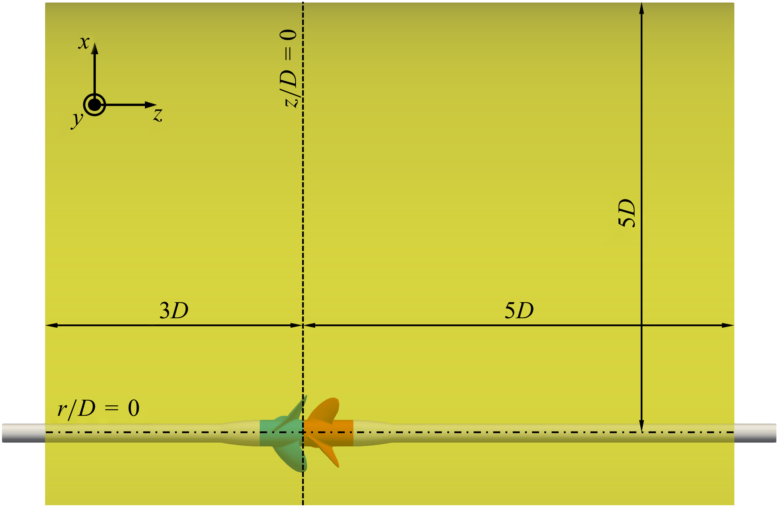


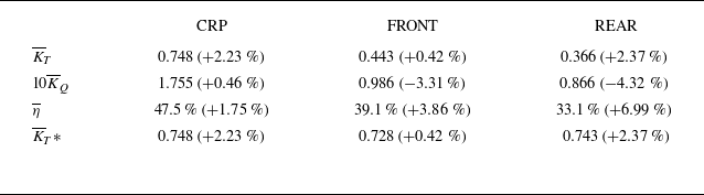
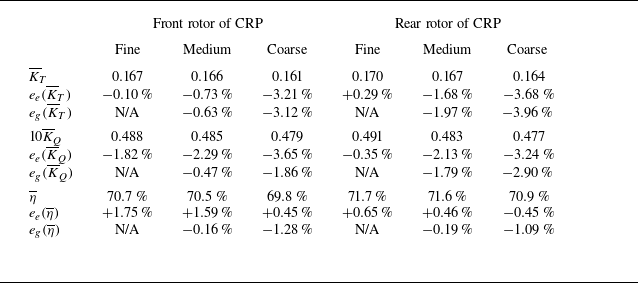

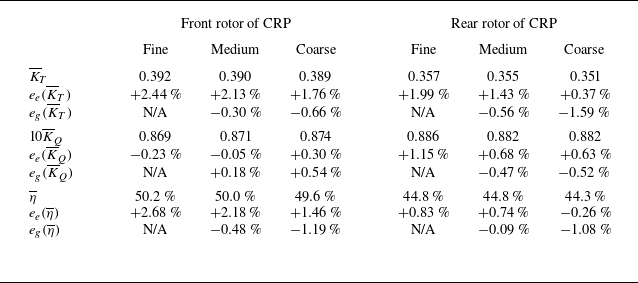

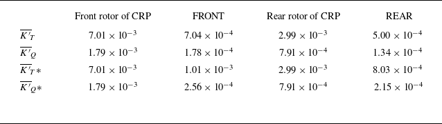
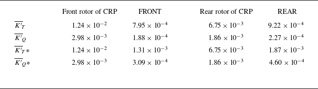


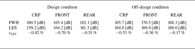


 Open access