


1. Introduction
Drop impact is pivotal in a wide range of fluid applications such as printing (Lohse Reference Lohse2022), hydrophobic coatings (Gauthier et al. Reference Gauthier, Symon, Clanet and Quere2015), ice formation on aeroplanes (Khojasteh et al. Reference Khojasteh, Kazerooni, Salarian and Kamali2016), disease spread (Bourouiba Reference Bourouiba2021), cooling (Breitenbach, Roisman & Tropea Reference Breitenbach, Roisman and Tropea2018; Aksoy et al. Reference Aksoy, Zhu, Eneren, Koos and Vetrano2021), atomized sprays (Villermaux Reference Villermaux2007; Moreira, Moita & Panao Reference Moreira, Moita and Panao2010), and microphysics processes in clouds and aerosols (Carslaw et al. Reference Carslaw2013), to name a few. Splashing from drop impact is defined as the generation of additional smaller droplets following the initial impact, called secondary droplets. One of the outstanding challenges in drop impact research is understanding the various processes affecting the characteristics of secondary droplets (Liang & Mudawar Reference Liang and Mudawar2016).
The focus here is on the transfer of mass during the impact of a drop with a film that is much thinner than the drop's diameter. When a drop impact event is sufficiently energetic, sheet-like jets form that typically are axisymmetric at onset but may later break symmetry and fragment into secondary droplets. Multiple distinct jets have been identified, distinguished by the time scale at which they emerge, their formation mechanism, and their characteristics (Yarin Reference Yarin2006). The so-called ejecta jet (Weiss & Yarin Reference Weiss and Yarin1999; Thoroddsen Reference Thoroddsen2002) emerges within tens of microseconds after impact, displays speeds many times that of the drop, and is thought to be produced by an overpressure condition (Weiss & Yarin Reference Weiss and Yarin1999; Davidson Reference Davidson2002; Howison et al. Reference Howison, Ockendon, Oliver, Purvis and Smith2005). A single impact event may produce several generations of ejecta jets (Zhang et al. Reference Zhang, Toole, Fezzaa and Deegan2012). The so-called corolla (sometimes called the lamella, crown, corona or Peregrine sheet) emerges on the time scale commensurate with the merger time of the drop and film (approximately 1 ms); its speed is close to the drop speed, and it is thought to be produced by a collision of the liquid from the drop with that of the film (Peregrine Reference Peregrine1981; Yarin & Weiss Reference Yarin and Weiss1995), causing an upward deflection of the combined fluid that leads to an axisymmetric sheet-like jet as shown in figure 4. As the corolla grows, its leading edge destabilizes and ultimately fragments into secondary droplets. Whereas ejectas and corollas are sheet-like jets resulting from the impact, another jet characterized by its spike-like shape, called the Worthington jet, forms from the collapse of the cavity in the film produced by the impact event. Whether a particular jet manifests depends on the fluid and kinematic parameters. We restricted our simulation to events in which the corolla is the only jet that forms.
Due to its importance in practical applications, drop impact has been studied extensively, revealing the phenomenology of splashing (Worthington & Cole Reference Worthington and Cole1897; Rein Reference Rein1993; Xu Reference Xu2007; Deegan, Brunet & Eggers Reference Deegan, Brunet and Eggers2008), and its dependence on multitudinous experimental conditions such as temperature (e.g. Aziz & Chandra Reference Aziz and Chandra2000; Tran et al. Reference Tran, Staat, Prosperetti, Sun and Lohse2012; Liang & Mudawar Reference Liang and Mudawar2017), surface preparation (e.g. Marengo et al. Reference Marengo, Antonini, Roisman and Tropea2011; Josserand & Thoroddsen Reference Josserand and Thoroddsen2016), additives (e.g. Aksoy et al. Reference Aksoy, Zhu, Eneren, Koos and Vetrano2021), incidence angle, tangential speed (e.g. Castrejón-Pita et al. Reference Castrejón-Pita, Muñoz-Sánchez, Hutchings and Castrejón-Pita2016), and many more (Liang & Mudawar Reference Liang and Mudawar2016). By comparison, the question about what parts of the drop and film contribute to a splash has received less attention (for exceptions, see e.g. Stumpf et al. Reference Stumpf, Ruesch, Roisman, Tropea and Hussong2022; Fudge et al. Reference Fudge, Cimpeanu, Antkowiak, Castrejón-Pita and Castrejón-Pita2023; Stumpf et al. Reference Stumpf, Roisman, Yarin and Tropea2023). Answering this question may lead to new techniques for controlling environmental transport phenomena, encapsulation and coating technology.
In this paper, we identify the fluid elements in the drop and film that are transferred to the corolla at different times. Investigating this transfer experimentally is challenging (see e.g. Stumpf et al. Reference Stumpf, Ruesch, Roisman, Tropea and Hussong2022), so instead we use high-resolution two-phase numerical axisymmetric simulations for multiple Reynolds and Weber numbers and film thicknesses. The imposition of axisymmetry is consistent with the experimental observation that corollas are typically axisymmetric at early times. We find a number of remarkable features: the mass of fluid in the drop that ultimately enters the corolla is confined to a thin surface layer, and most surprisingly its characteristic dimensions are almost entirely determined by the thickness of the film rather than by a combination of Weber and Reynolds numbers, as one might expect based on extensive prior work characterizing splashing (see e.g. Mundo, Sommerfeld & Tropea Reference Mundo, Sommerfeld and Tropea1995; Rioboo et al. Reference Rioboo, Bauthier, Conti, Voue and De Coninck2003; Josserand & Zaleski Reference Josserand and Zaleski2003; Deegan et al. Reference Deegan, Brunet and Eggers2008; van der Veen et al. Reference van der Veen, Tuan, Lohse and Sun2012).
In § 2, we present our numerical methods, the simulation configuration, its validation, and our parameter space, and the post-processing techniques to identify the corolla and to track the fluid elements entering it. In § 3, we present a series of maps showing the domains of fluid elements that will go on to form the corolla at various later times. The most salient features of these maps are the shape and scaling properties of the domains. We show that the shape scales with the depth of the film but is almost independent of the Weber and Reynolds numbers. In § 4, we discuss the various theories proposed for crown formation, and their relevance and applicability to the maps.
2. Methods
2.1. Numerical method
Numerical treatments of wet drop impact in two and three dimensions have been developed extensively. Harlow & Shannon (Reference Harlow and Shannon1967) conducted some of the first numerical computations using an axisymmetric code that neglected surface tension. Weiss & Yarin (Reference Weiss and Yarin1999), and later Davidson (Reference Davidson2002), used the boundary integral method on an axisymmetric domain and an inviscid formulation of the dynamics to show the existence of a jet preceding the corolla, the so-called ejecta jet. Rieber & Frohn (Reference Rieber and Frohn1999) were the first to perform fully three-dimensional computations using a volume-of-fluid method, and argued that the instability of the corolla is due to the Rayleigh instability. Currently, drop impact simulations can be performed routinely and reliably using open source software such as Gerris and Basilisk (Thoraval et al. Reference Thoraval, Takehara, Etoh, Popinet, Ray, Josserand, Zaleski and Thoroddsen2012; Agbaglah & Deegan Reference Agbaglah and Deegan2014; Josserand, Ray & Zaleski Reference Josserand, Ray and Zaleski2016), particularly when supplemented by experimental results as we do here. Axisymmetric computations are readily realized on reasonably sized clusters. While in principle fully three-dimensional computations are possible, they continue to strain resources, and the issues of numerical artefacts arising from changes in topology are not fully resolved (see e.g. Afanador et al. Reference Afanador, Zaleski, Tryggvason and Lu2021; Zhou et al. Reference Zhou2021).
We model a gas–liquid system with the incompressible Navier–Stokes equation, utilizing the one-fluid approach:
 $$\begin{gather} \rho (\partial_t \boldsymbol{u}+\boldsymbol{u} \boldsymbol{\cdot} {\boldsymbol{\nabla}} \boldsymbol{u}) ={-} {\boldsymbol{\nabla}} p + {\boldsymbol{\nabla}} \boldsymbol{\cdot} (2\mu \boldsymbol{\mathsf{D}}) + \gamma \kappa \delta_s \boldsymbol{n}, \end{gather}$$
 $$\begin{gather}{\boldsymbol{\nabla}} \boldsymbol{\cdot} \boldsymbol{u}= 0, \end{gather}$$
where  $\boldsymbol {u}$ is the velocity of the fluid, $\mu \equiv \mu (\boldsymbol {x}, t)$ is the viscosity, $\rho \equiv \rho (\boldsymbol {x}, t)$ is the density, and $\boldsymbol{\mathsf{D}}$ is the deformation tensor. The densities and viscosities are constant in each phase, with values $\rho _g$ and $\mu _g$ in the gas, and $\rho _l$ and $\mu _l$ in the fluid. The surface tension term acts only at the interface and is included in (2.1) by a Dirac function $\delta _s$, with prefactors $\kappa$ and $\boldsymbol {n}$ denoting the local curvature and normal unit vector to the interface, respectively.
We use the Basilisk open-source solver (Popinet Reference Popinet2018), which is an enhanced version of the Gerris solver widely used for various multiphase flow problems (Agbaglah et al. Reference Agbaglah, Delaux, Fuster, Hoepffner, Josserand, Popinet, Ray, Scardovelli and Zaleski2011, Reference Agbaglah, Thoraval, Thoroddsen, Zhang, Fezzaa and Deegan2015; Thoraval et al. Reference Thoraval, Takehara, Etoh, Popinet, Ray, Josserand, Zaleski and Thoroddsen2012; tao Li et al. Reference tao Li, Li, Zong and Chen2014; Visser et al. Reference Visser, Frommhold, Wildeman, Mettin, Lohse and Sun2015; Ling et al. Reference Ling, Fullana, Popinet and Josserand2016; Osama et al. Reference Osama, Deng, Thoraval and Agbaglah2022). In Basilisk, the liquid–gas interface is tracked by the volume-of-fluid method on an octree structured grid facilitated by adaptive mesh refinement. The adaptive mesh refinement in this study relies on a criterion of wavelet-estimated discretization error (Van Hooft et al. Reference Van Hooft, Popinet, Van Heerwaarden, Van der Linden, de Roode and Van de Wiel2018). To define physical properties such as  $\mu$ and $\rho$, the volume fraction of the liquid phase $f$ is utilized to linearly interpolate these quantities in cells containing the liquid–gas interface:
 $$\begin{gather} \mu(f)= f\mu_l + (1-f)\mu_g, \end{gather}$$
 $$\begin{gather}\rho(f)= f\rho_l + (1-f)\rho_g. \end{gather}$$
The transport equation of  $f$ is computed from
 \begin{equation} \partial_t{f} + {\boldsymbol{\nabla}}\boldsymbol{\cdot}(\boldsymbol{u}f)= 0. \end{equation}
Basilisk uses a balanced-force technique to calculate the surface tension, and the interface's curvature is determined using the height function approach. Further elaboration on the numerical methods utilized in Basilisk can be found in Popinet (Reference Popinet2003, Reference Popinet2009).
2.2. Numerical simulations
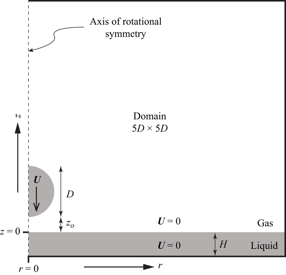
We modelled a spherical drop with initial diameter  $D$ and velocity $U$ impacting a film of the same liquid with thickness $H$ as shown in figure 1. The computational domain was $5D \times 5D$ in size, and axially symmetric with the axis of symmetry along the vertical centreline of the drop. No-slip boundary conditions were enforced on the top, bottom and right-hand edges of the domain. The grid was discretized using adaptive mesh refinement with minimum spacing $5D/2^{14}$ along each dimension. This level of refinement corresponds to a minimum mesh size $\Delta x=D/3277$, and was shown previously to accurately represent experimental results (Agbaglah & Deegan Reference Agbaglah and Deegan2014) as shown in figure 2. The simulations were initialized with the drop's bottom at a vertical distance $0.001D$ above the film's upper surface, and with a velocity field equal to $-U\boldsymbol {z}$ within the drop, and zero everywhere else.
A spherical drop of diameter  $D$ falls vertically through a gas with speed $U$ and collides with a film of thickness $H$ of the same liquid. Initially, the velocity is zero everywhere except in the drop, and the drop is at a vertical distance $z_o=10^{-3}D$ above the film surface. The simulations were performed on an axisymmetric domain $5D\times 5D$, with the dashed line as the axis of symmetry. No-slip boundary conditions were enforced on the other three boundaries.
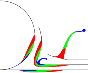
Comparison of X-ray images of drop impact on a deep pool (greyscale images) and the corresponding snapshot from numerical simulations with the same dimensionless parameters: (a i,ii)  ${\textit {We}} = 324$, ${\textit {Re}} = 2191$; (b i,ii) ${\textit {We}} = 451$, ${\textit {Re}} = 710$. Adapted from Agbaglah & Deegan (Reference Agbaglah and Deegan2014).
The system is characterized by five dimensionless groups: the Reynolds number  ${\textit {Re}}=\rho _{l} U D/ \mu _{l}$, the Weber number ${\textit {We}} = \rho _{l} U^{2} D/\sigma$, the dimensionless thickness $h\equiv H/D$, and the ratios of the liquid and gas dynamic viscosity $\varLambda =\mu _{l}/\mu _g$ and density $\rho _{l}/\rho _{g}$. We fixed the values of $D=0.2$ cm, $U=190\,{\rm cm}\,{\rm s}^{-1}$, $\rho _l=0.851\,{\rm g}\,{\rm cm}^{-3}$, $\rho _g=1.293\times 10^{-3} \,{\rm g}\,{\rm cm}^{-3}$, $\mu _g=1.90\times 10^{-2}$ cP, and varied $\mu _l$, $\sigma$ and $H$ to tune the values of ${\textit {Re}}$, ${\textit {We}}$ and $h$, respectively. All results below are reported in dimensionless units, where lengths are scaled by $D$ and times by $D/U$.
The ranges of values for the Weber number, Reynolds number and dimensionless thickness in our study were chosen to focus exclusively on impact events that produce a corolla without a separate ejecta – i.e. events such as in figure 2(a) rather than figure 2(b) – while remaining close to  ${\textit {Re}}=2191$, ${\textit {We}}=324$ where we can validate our simulations. The constraints are illustrated schematically in figure 3 in the ${\textit {Re}}$– ${\textit {We}}$ plane; the boundaries depicted therein shift with depth.
Qualitative phase diagram for the type of splash observed. The boundaries vary with depth, but the overall structure remains the same (Cossali, Coghe & Marengo Reference Cossali, Coghe and Marengo1997; Rioboo et al. Reference Rioboo, Bauthier, Conti, Voue and De Coninck2003; Thoraval et al. Reference Thoraval, Takehara, Etoh, Popinet, Ray, Josserand, Zaleski and Thoroddsen2012; Agbaglah et al. Reference Agbaglah, Thoraval, Thoroddsen, Zhang, Fezzaa and Deegan2015). Our simulations focus on impact events that produce only a corolla as in (a)  ${\textit {Re}} = 1000$, ${\textit {We}}=500$, $h=0.025$, $t=0.6$ and (b) ${\textit {Re}} = 2042$, ${\textit {We}}=292$, $h=0.025$, $t=1.05$. The flows outside of the corolla regime are (c) ${\textit {Re}} = 2000$, ${\textit {We}}=100$, $h=0.2$, $t=0.3$, (d) ${\textit {Re}} = 3000$, ${\textit {We}}=500$, $h=0.2$, $t=0.3$, (e) ${\textit {Re}} = 2042$, ${\textit {We}}=292$, $h=0.4$, $t=0.7$.

Higher values of  $h$ combined with low ${\textit {We}}$ and high ${\textit {Re}}$ tend to produce a separate ejecta; we observed, for example, that at $h=0.4$ for ${\textit {Re}}=2042$ and ${\textit {We}}=292$, an ejecta is present. Thus we limited $h\leq 0.2$. Low values of $h$ are difficult to achieve experimentally (see e.g. Wang & Chen Reference Wang and Chen2000). For example, $h=0.015$ corresponds to a 30 $\mathrm {\mu }$m film for a 2 mm drop. Moreover, qualitatively different flows appear after some time at low values of $h$, such as the one shown in figure 4(f). Thus we limited $h\geq 0.015$.
Defining the corolla. (a) Simulation with  ${\textit {Re}}=1000$, ${\textit {We}}=292$, $h=0.05$ at $t=0.2$, with the interface in red, and the fluid originally in the drop and film in blue and white, respectively. (b) Magnified view of the corolla, with markers used to define its boundaries. Point ${\rm A}$ is the local minimum in $z$ of the interface $(r,z)$ nearest $r=0$. Point ${\rm C}$ is found by iteratively rotating anticlockwise a vertical line through point ${\rm A}$ until it meets the interface. (c–f) Problematic surface profiles. (c) For thick films at late times ( $h=0.2$ at $t=0.9$ shown), point ${\rm A}$ falls below the film's initial surface height, and it is no longer possible to construct a tangent. (d–f) Surface profiles for ${\textit {Re}}=1000$, ${\textit {We}}=292$, $h=0.025$ at $t = 0.5, 0.8, 0.995$, illustrating the appearance of multiple minima.

Low Weber numbers are insufficiently energetic to produce a corolla, but too large a value produces a separate ejecta (Agbaglah et al. Reference Agbaglah, Thoraval, Thoroddsen, Zhang, Fezzaa and Deegan2015). For example, with  ${\textit {We}}= 100$, ${\textit {Re}}=1000,2000,3000$ and $h=0.03,0.05,0.2$, a corolla does not form. At higher values of the Reynolds and Weber numbers, the corolla begins to interact with the drop (see ‘bumping’ and other phenomena in Thoraval et al. Reference Thoraval, Takehara, Etoh and Thoroddsen2013). We observed bumping at ${\textit {Re}}=3000$, ${\textit {We}}=500$, $h=0.2$. Thus we settled on the ranges $500\geq {\textit {We}}\geq 100$ and $3000\geq {\textit {Re}}\geq 1000$.
Since the dependence on the density and viscosity ratios between the gas and liquid is almost insignificant for the range of values in typical experiments, these were not varied systematically. The density ratio was fixed at 709 for all simulations, and the viscosity ratio changed with  ${\textit {Re}}$.
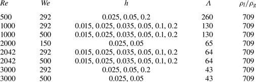
The parameter values for all 34 simulations are listed in table 1. Each simulation (i.e. a single combination of  $({\textit {Re}}, {\textit {We}}, h)$) took approximately two days on 32 cores (1536 CPU hours), using Basilisk's parallelization capabilities and adaptive mesh refinement, and required up to 0.5 TB of storage for the output files. Post-processing to backtrack the fluid elements (see algorithm below) required up to an additional three days on a single core, and 62 GB of random access memory.
Parameters for numerical simulations.
The main advantage of an axisymmetric simulation is the modest computational resources needed, when compared to those needed in a three-dimensional domain. The latter would require, using the adaptive mesh refinement, roughly  $1.6 \times 10^6$ CPU hours and 3 PB of disk space per set of $({\textit {Re}}, {\textit {We}})$. Given the number of simulations and the resources available to us, performing our study in three dimensions was infeasible. A downside of an axisymmetric simulation of drop impact is that it cannot reproduce the longitudinal destabilization of the corolla's edge that ultimately produces secondary droplets. This disadvantage is somewhat mitigated by the well-known difficulties of resolving droplet pinch-off in three dimensions (Afanador et al. Reference Afanador, Zaleski, Tryggvason and Lu2021; Zhou et al. Reference Zhou2021), and experiments show that the corolla is approximately axisymmetric for times less than $D/U$ (i.e. $t<1$) for the parameter range of our study.
2.3. Defining the corolla
Physical experiments in the parameter regime of our study (table 1) produce an initially axisymmetric corolla that ultimately breaks up into secondary droplets. The corolla in our simulations appears in cross-section as a thin strip of fluid rising from where the drop and film meet, as shown in figure 4(a). Unlike in experiments, corolla break-up is not possible because of the imposed axial symmetry.
Dividing the liquid domain into parts inside and outside the corolla proved challenging since no criteria that we tried based on identifiable features on the interface, velocity or vorticity field worked for all parameters and all times. Ultimately, we adopted the criteria shown in figure 4(b), because this worked with the greatest number of simulations. We define point  ${\rm A}$ to be the first minimum of the interface height encounter moving along the interface, starting from the centre of the drop. Next, we found the line segment through point ${\rm A}$ and tangent to the interface on the other side of the corolla, as shown in figure 4(b). Any fluid inside the curve composed of the interface between points ${\rm A}$ and ${\rm C}$ and the line segment ${\rm AC}$ is defined to be in the corolla.
This definition for the boundary of the corolla always works at short times, but breaks down under two different conditions at late times. For thick films, the vertical position of point  ${\rm A}$ decreases and ultimately falls below the undisturbed height of the film (or equivalently, its position at infinity), and thereafter the tangent curve no longer exists (see figure 4c). For the thinnest films at late times, multiple minima appear between the drop centre and the corolla's tip, as shown by the sequence in figures 4(d–f), so point ${\rm A}$ fails to be unique. Selecting the first minimum leads to an unappealing definition of the corolla, and switching to the second minimum (say, when it falls below the first) leads to a discontinuity of the mass inside the corolla. Overall, our definition of the corolla's boundary works in approximately 80 % of the parameter–time combinations, which is better than any other definition that we tried.
2.4. Lagrangian tracking of the fluid elements
We computed the Lagrangian trajectories of fluid elements from the flow calculation to determine if a particular element is inside or outside the corolla at some particular future time. It proved more accurate to compute the trajectories backwards in time, starting with the elements position in the corolla and tracing its origin back to  $t=0$ (Dubitsky, Mcrae & Bird (Reference Dubitsky, Mcrae and Bird2023) employed a similar technique). First, the Basilisk output files were post-processed using Python's shapely.geometry module to identify every mesh point inside the corolla at 0.1 time increments from 0.1 to $0.9$. Next, the backwards-in-time trajectory of each mesh point was computed using the time-reversed flow field stored in the output files from Basilisk with time resolution $\delta t\equiv 5\times 10^{-4}$. The first two time steps were computed using a first-order Euler method with time-step size $\delta t$. These data were then used to initialize a third-order Adams–Bashforth scheme for the subsequent steps, tracing the elements position back to $t=0$. Thus the trajectory for each mesh point for each of the nine starting times is computed separately. The algorithm applied to one particular start time yields a sequence such as that shown in figure 5. The final frame of this sequence is an example of the main result of our computations: it shows the domain of fluid elements prior to impact that will form the corolla at some later time, $t=0.5$ in this particular case.
Backtracking. Simulation snapshots for  ${\textit {Re}}=1000$, ${\textit {We}}=292$, $h=0.2$, with the interface shown as a black line, and the tracers placed inside the corolla shown in red and blue at (a) $t=0.5$. (b–d) The advection of the tracers at $t = 0.3, 0.1, 0.0$. The tracers are coloured red or blue to indicate their ultimate destination in the drop or the film, respectively.

A few trajectories near the liquid–air interface or the computational domain boundary stray across these boundaries. Since this unphysical behaviour is caused by the finite time-step size in our backtracking algorithm and was infrequent, we discarded such trajectories. This elimination scheme was employed most often for the thinnest films, and was most acute for mesh points that begin near the bottom solid boundary. In the most adverse case ( ${\textit {Re}}=2042$, ${\textit {We}}=292$, $h=0.015$), this occurred for approximately $3\,\%$ of tracers.
3. Results
We follow the Lagrangian path of fluid elements in the drop or film starting at  $t=0$, and determine if it ends up in the corolla at some particular time $t>0$. By tracing all such elements, we construct domains of fluid elements that ultimately enter the corolla. These domains at any given time consist of two disjoint subdomains: one for the drop and one for the film, since both contribute to the corolla. Examples of these domains are shown in figure 6, colour-coded to indicate the time when they entered the corolla. We refer to these diagrams as maps since they show which parts of the drop and film will evolve into the corolla.
Mass transfer maps for  ${\textit {Re}}=1000$, ${\textit {We}}=292$ and $h$ values (a) $0.2$, (b) 0.1, (c) 0.05, (d) 0.035, (e) 0.025, (f) 0.015. The colours identify elements that enter the corolla prior to $t$ values $0.1$ (purple), 0.2 (red), 0.3 (dark blue), 0.4 (yellow), 0.5 (green), 0.6 (orange), 0.7 (cyan), 0.8 (pink), 0.9 (brown). There are fewer data points in (e,f) because of the ambiguity in delineating the corolla, as discussed in the text and figure 4.

The main qualitative features of these maps are: (i) the fluid contribution from the drop to the corolla comes from a narrow sliver on the surface of the drop starting near its south pole; (ii) the shapes of the domains in the drop are generally similar in appearance, having a comma-like shape; (iii) the percentage of mass contributed by the film versus the drop changes with film thickness, with the drop contribution dominating for the thinnest films; and (iv) the mass contribution from the film comes from all depths for the thinnest films. Below, we quantify these observations and show that drop domains have a self-similar shape.
We characterized the domains by their lengths  $L_d$ and $L_f$, thicknesses $W_d$ and $W_f$, and volumes $V_d$ and $V_f$, as illustrated in figure 7. The subscripts denote drop ( $d$) and film ( $\,f$). In order to measure domains inside the drop, it is convenient to unroll its shape with polar coordinates so that positions $(r,z)$ in the simulation are mapped to $\rho =\sqrt {r^2+(z_c-z)^2}$ and $\tan \theta = r/(z_c-z)$, where $(0,z_c)$ is the position of the drop's centre at $t=0$.
(a) Domains of fluid elements backtracked to  $t=0$ from $t = 0.9$ for ${\textit {Re}}= 1000$, ${\textit {We}}=292$, $h=0.1$. The dashed lines correspond to the drop surface (curved) and the film surface (upper flat) and the bottom boundary (lower flat). We extract the quantities $L_d$ and $W_d$ corresponding to the length and thickness of domains in the drop, and similarly $L_f$ and $W_f$ for the film. (b) Drop domain mapped to polar coordinates, where $W_d$ is defined as the radial difference between the surface at $\rho =R$ and the tracer closest to the centre of the drop. (c) Film domain, where $W_f$ is defined as the distance between the film surface and the deepest tracer. The black solid lines in (b,c) are the domain boundaries used to compute their volumes in the drop ( $V_d$) and the film ( $V_f$), factoring in the cylindrical geometry.

Figure 8 shows a plot of the length of the drop domain versus time for all 34 simulations. Surprisingly, there is little variation in the magnitude of this quantity with any of the simulation parameters  ${\textit {Re}}$, ${\textit {We}}$, $h$. The small variation correlates most strongly with $h$: following any one colour (corresponding to fixed ${\textit {Re}}$ and ${\textit {We}}$) in figure 8(b) shows a 2–4 % variation, whereas following any one symbol (corresponding to fixed $h$) in figure 8 shows variation of at most 1 %. Henceforth, we adopt $L_d$ rather than time as a measure of the impact event's progress.
(a) Plot of  $L_d$ versus $t$ for all 34 simulations. A fit to $B{(t-t_o)^{\xi }}$ is overlaid on the data (red dashed line), with $B=0.96$, $t_o=0.032$, $\xi =0.35$. (b) Plots of $\%\Delta L_d\equiv (L_d/\overline {L_d}-1)$ at $t=0.3$ versus (i) $h$, (ii) ${\textit {We}}$, (iii) ${\textit {Re}}$. Combinations of ${\textit {Re}}$ and ${\textit {We}}$ are indicated by colour: green for ${\textit {Re}}=2042$, ${\textit {We}}=292$; red for ${\textit {Re}}=1000$, ${\textit {We}}=500$; blue for ${\textit {Re}}=1000$, ${\textit {We}}=292$; grey for ${\textit {Re}}=2042$, ${\textit {We}}=500$; yellow for ${\textit {Re}}=3000$, ${\textit {We}}=292$; fuchsia for ${\textit {Re}}=3000$, ${\textit {We}}=292$; cyan for ${\textit {Re}}=500$, ${\textit {We}}=292$; purple for ${\textit {Re}}=2000$, ${\textit {We}}=150$. Thickness $h$ is indicated by symbols: $\triangleright$ for 0.015, $\diamond$ for 0.025, $\circ$ for 0.035, $\Box$ for 0.05, $\vartriangle$ for 0.1, $\triangledown$ for 0.2. See supplementary material figure S4 available at https://doi.org/10.1017/jfm.2024.766.
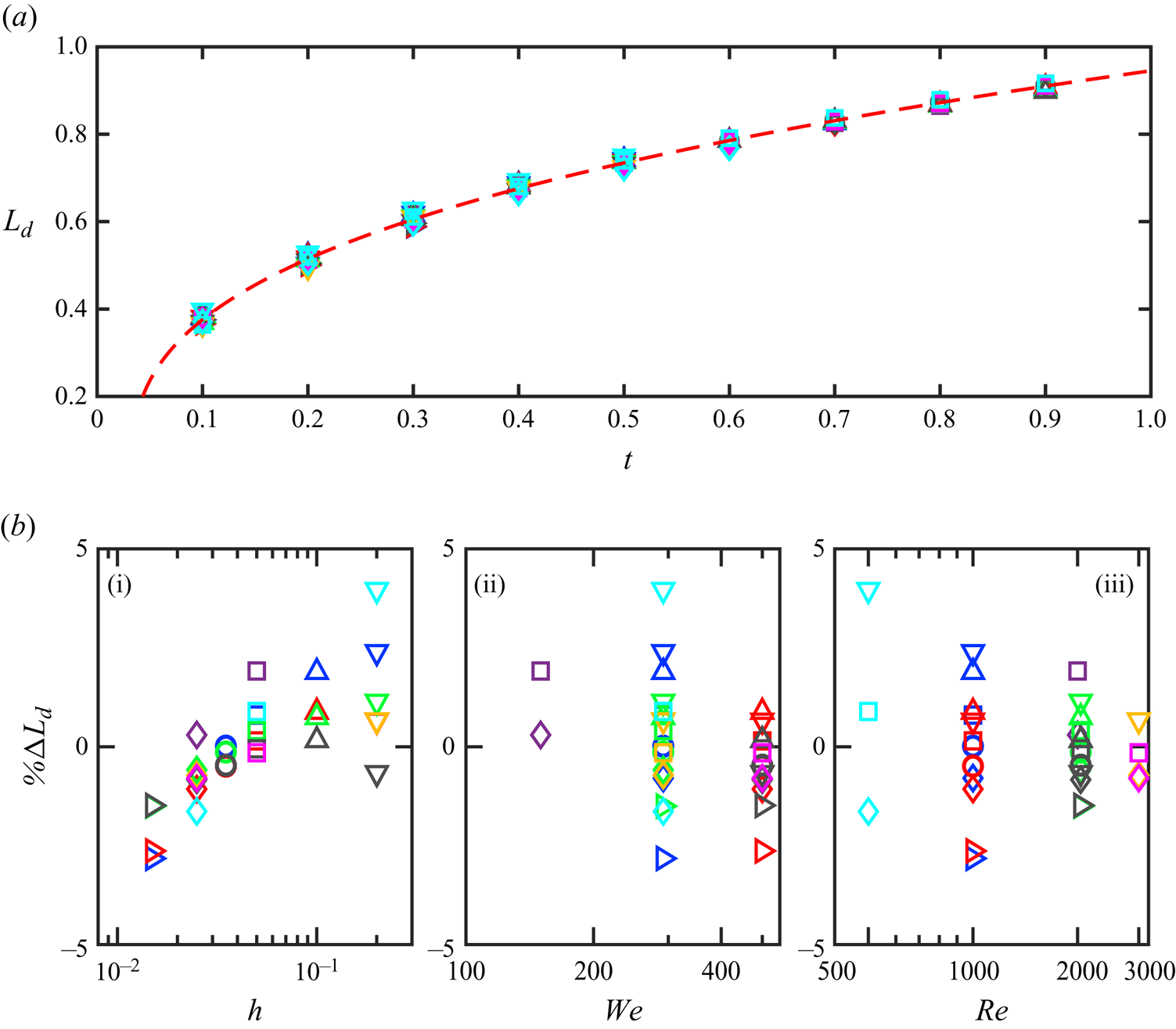
Figure 9(a) is a plot of  $W_d$ versus $L_d$ that includes all the simulations in our study. Around any fixed value of $L_d$, or equivalently at a fixed time after impact, $W_d$ shows large variation. As an example, for $L_d\approx 0.6$ shown in the inset of figure 9(a), $W_d$ varies by 100–200 %. Figure 9(c) plots these variations versus $h$,
$h$,  ${\textit {We}}$ and ${\textit {Re}}$, showing that they are primarily due to $h$.
$h$.
(a) Width versus length of drop domain, with the inset showing the same for  $t=0.3$ only. (b) Data in (a) scaled with $h$ using the form of (3.1) with $\alpha =5/8$ and $\beta =1/4$. The red line is the best fit to a power law, yielding prefactor 0.059 and exponent 3.6. (c) Data at a fixed time (inset in a) plotted versus (i) $h$, (ii) ${\textit {We}}$, (iii) ${\textit {Re}}$. Symbols and colours are as in figure 8.

The same case can be made for the other parameters,  $W_f, V_d, V_f, L_f$. The lack of sensitivity to ${\textit {We}}$ and ${\textit {Re}}$ suggests searching for a collapse of the data with a scaling relationship that depends only on $h$, of the form
 \begin{equation} y=h^{\alpha}f\left(L_dh^{-\beta}\right), \end{equation}
where  $f(\cdot )$ is an arbitrary function (Barenblatt Reference Barenblatt2003). Such a scaling exists and is shown for $W_d$ in figure 9(b), for $V_d, W_f, V_f$ in figure 10, and for $L_f$ in figure 11.
(a) Volume versus length of drop domain. (b) Same data as in (a) plotted with scaled variables with  $\beta =1/4$ and $\alpha =1$. The red line is the best fit to a power law, yielding prefactor 0.071 and exponent 5.1. (c) Width of drop domain versus length of drop domain. (d) Same data as in (c) plotted with scaled variables with $\beta =1/4$ and $\alpha =1$. (e) Volume of drop domain versus length of drop domain. (f) Same data as in (e) plotted with scaled variables with $\beta =1/4$ and $\alpha =7/4$. Symbols and colours are as in figure 8.

(a) Raw data for film length versus drop length. (b) Same data as in (a) on a log-log plot with different thicknesses shifted arbitrarily to better display their trends. (c) Scaling of data with  $\alpha =-5/8$, $\beta =-1/2$. Symbols and colours are as in figure 8.

Rescaling  $W_d$ and $V_d$ results in the data from all simulations collapsing onto a straight line on a log-log plot. Fits to a power law yield
 $$\begin{gather} W_d=0.058 h^{5/8} (L_d h^{{-}1/4})^{3.6}=0.058 h^{{-}0.28}L_d^{3.6} \sim h^{{-}0.28} (t-t_o)^{1.3}, \end{gather}$$
 $$\begin{gather}V_d=0.071 h (L_d h^{{-}1/4})^{5.1}=0.071 h^{{-}0.28}L_d^{5.1} \sim h^{{-}0.28}(t-t_o)^{1.8}, \end{gather}$$
where the time dependence follows from  $L_d\sim (t-t_o)^{0.35}$. Rescaling $W_f$ and $V_f$ results in the data from all simulations collapsing onto a single curve, but the functional form is not readily apparent. These data give scaled forms
 $$\begin{gather} W_f=h F (L_d h^{{-}1/4}), \end{gather}$$
 $$\begin{gather}V_f=h^{7/4} G(L_d h^{{-}1/4}), \end{gather}$$
 Here,  $L_f$ differs significantly from other domain parameters. As shown in figure 11, for thinner films $L_f\propto L_d$, but not for thicker films ( $h\ge 0.1$). It is possible to collapse these data (see figure 11c), but the rescaling differs from that of other parameters. Considering the evolution of film domains in figure 6, one sees that they do not span the full depth of the film in thicker cases, suggesting that the solid substrate constrains the growth of the film domain for thinner films, and leads to qualitatively different growth in the two different limits.
The results for the fluid entrained into the bulb of the corolla,  $V_{frac}$ (ratio of the volume of liquid from the drop to the total volume of the bulb), were compared to those of Stumpf et al. (Reference Stumpf, Ruesch, Roisman, Tropea and Hussong2022), who measured the secondary droplet composition. Since our axisymmetric simulation does not produce droplets, we approximated the composition of the droplet by measuring the composition of the bulb at the end of the corolla. We define the bulb to begin where the corolla develops a neck as the beginning of the liquid torus that would fragment into droplets. For $Re=2042$, $We=500$, $h=0.2$ at $t=0.5$, we observed $V_{frac}=0.23$ inside the bulb, which is within the observed range in Stumpf et al. (Reference Stumpf, Ruesch, Roisman, Tropea and Hussong2022, figure 14).
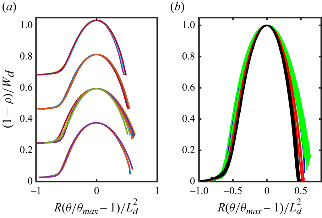
In addition to the power-law scaling of the characteristics of the domain in the drop, we find that the shape tends to a self-similar limit. Figure 12 plots the scaled domain boundaries, in polar coordinates as in figure 7, from all simulations with  $h=0.2$. We scale the raw shape $(\theta,\rho )$, which generally displays a single peak, by normalizing the peak height ( $\rho \rightarrow (1-\rho )/W_d$), zeroing the peak position $\theta \rightarrow 1-\theta /\theta _{max}$, where $\theta _{max}$ is the angular position of the peak, and scaling the peak width by $L_d^{2}$. As shown in figures 12(a,b), the domain shape evolves towards the same shape irrespective of the Weber and Reynolds numbers in these scaled coordinates. We take the shape at $t=0.9$ and $h=0.2$ to be representative of the asymptotic form of the domain shape (see figure 12c), and compare this with the other depths in figure 13. These data suggest that all depths tend towards the same asymptotic form.
Profiles of the drop domains for  $h=0.2$ for all ${\textit {Re}}$, ${\textit {We}}$, and times shifted and scaled according to the formulas in the axis label so that their peaks coincide. (a) Profiles at different times shifted vertically for clarity with the topmost curve corresponding to $t=0.1$, the next one down to $t=0.2$, and so on up to $t=0.9$. (b) Same data as in (a) without the vertical offset. (c) Data for all five profiles at $t=0.9$.

Profiles of the drop domains for all  ${\textit {Re}}$, ${\textit {We}}$ and $h$ at $t=0.9$ shifted and scaled according to the formulas in the axis label so that their peaks coincide. (a) Profiles for different film thicknesses shifted vertically for clarity, with topmost to bottommost corresponding respectively to $h=0.2, 0.1, 0.05, 0.025$. (b) Same data as in (a) without the vertical offset.
4. Summary and discussion
The corolla is composed of fluid that comes from both the drop and the pool. This is well-established fact corroborated by computations (e.g. Josserand & Zaleski Reference Josserand and Zaleski2003), experiments (e.g. W. van Hoeve, T. Segers, H. Kroes, D. Lohse & M. Versius, A splash of red, private communication 2011; Versluis Reference Versluis2013), and theory (e.g. Cooker & Peregrine Reference Cooker and Peregrine1995; Howison et al. Reference Howison, Ockendon, Oliver, Purvis and Smith2005). Recent work, particularly for the case where the drop and film are different fluids, has focused on quantifying the volumetric contribution from the drop versus that from the film (Fudge et al. Reference Fudge, Cimpeanu, Antkowiak, Castrejón-Pita and Castrejón-Pita2023; Stumpf et al. Reference Stumpf, Ruesch, Roisman, Tropea and Hussong2022, Reference Stumpf, Roisman, Yarin and Tropea2023).
Using direct numerical simulations on an axisymmetric domain, we find that the fluid in the corolla at any moment of time produced by the impact of a spherical drop on a film comes from a thin layer on the drop's surface and a surface layer in the film that spans the film's full depth for thinner films. The novelty of our results is that they pinpoint the volume elements in each of the fluid bodies prior to impact from which the corolla is formed.
The shape of the domains that go on to form the corolla scales with the film thickness and is insensitive to the Weber and Reynolds numbers. A collapse of the data shows that the data for the drop domain are well modelled by a power law, and moreover, the boundary of the domain approaches a self-similar form. The contribution from the film also displays scaling with the thickness and insensitivity to the Reynolds and Weber numbers, but the collapsed data follow a more complex form that we attribute to the presence of a solid boundary beneath the film that limits the downward growth of the domain.
Our characterization would be useful for developing techniques to selectively disperse drop additives by seeding the parts of the drop that will later form the corolla. An advantage of this approach revealed by our study is that such a dispersal mechanism would be highly robust to variations of the Weber and Reynolds numbers.
The collapse of the scaled domains and their characteristics shows that their shape is predominantly governed by  $h$, and the dependence on ${\textit {We}}$ and ${\textit {Re}}$ is all but negligible. In contrast, we observe large changes in the time evolution of the corolla's shape, and base thickness and speed with variations in the Reynolds and Weber numbers (see e.g. figure 14). Moreover, much of the literature on splashing revolves around correlating splashing with the Reynolds or Weber numbers, or various combination of these two. To give just two examples: Rioboo et al. (Reference Rioboo, Bauthier, Conti, Voue and De Coninck2003) showed that ${\textit {We}}$ sets a minimum threshold for the formation of a jet, and Yarin & Weiss (Reference Yarin and Weiss1995) showed that ${\textit {We}}/{\textit {Re}}$ sets a threshold for splashing. Indeed, the most salient fact of drop impact is that speed matters: slow speeds lead to coalescence, and high speeds lead to splashing. The conundrum is how to reconcile changes in the time evolution of the corolla with ${\textit {Re}}$ and ${\textit {We}}$, and the seemingly invariance to these values of the fluid elements that form the corolla.
Comparison of interfaces for same depth  $h=0.025$ and time $t=0.3$ for ${\textit {Re}}=1000$, ${\textit {We}}=292$ (a) and ${\textit {Re}}=3000$, ${\textit {We}}=500$ (b). More comparisons are shown in supplementary material figure S3.

The independence of  $L_d$ from all simulation parameters suggests looking for a physical mechanism in the geometric length scales intrinsic to an impact event. The penetration depth $Ut/D$ (in unscaled units; just $t$ in scaled units) is clearly not going to work as it varies as $t$, whereas $L_d\sim t^{0.35}$. The next candidate is $L_g$, the arc length of the submerged portion of the drop if the drop passed like a ghost through the film, i.e. the arc length on a circle crossed by a line a distance $t$ from its apex:
 \begin{equation} L_g=\tfrac12\arccos(1-2t). \end{equation}
As shown in figure 15(a),  $L_g$ provides a reasonable description of the data, especially at early times.
(a) Plot of  $L_d$ versus $t$. The green curved line is $L_g(t)$, and the black straight line is $t$. (b) Comparison of $L_d$ and the crown radius $r_c$ for assumption $r_c=r_A$. Symbols and colours are as in figure 8.

As an alternative avenue to explain our results, we considered the kinematic discontinuity theory of Yarin & Weiss (Reference Yarin and Weiss1995). The central result of the theory is that the radial distance at which the corolla emerges from the film scales as  $h^{-1/4}$ but is otherwise independent of ${\textit {Re}}$ and ${\textit {We}}$ (Yarin & Weiss Reference Yarin and Weiss1995; Rieber & Frohn Reference Rieber and Frohn1999; Trujillo & Lee Reference Trujillo and Lee2001; Roisman & Tropea Reference Roisman and Tropea2002; Stumpf et al. Reference Stumpf, Roisman, Yarin and Tropea2023). The striking similarity to our observed scaling $h^{-0.28}$ (see (3.3)), and ${\textit {Re}}$ and ${\textit {We}}$ independence, suggest that the theory may account for our results.
To examine this possibility, we tested the hypothesis that  $L_d\propto r_c$, where $r_c$ is the radial distance of the kinematic discontinuity (Yarin & Weiss Reference Yarin and Weiss1995). Corollas always have a finite thickness, thus identifying $r_c$, which is a mathematical point in theory, is ambiguous. We tried two different schemes: (i) $r_c=r_A$ and (ii) $r_c=\frac 12(r_A+r_C)$, where $r_A$ and $r_C$ are the radial distances of points ${\rm A}$ and ${\rm C}$ in figure 4. Figure 15(b) shows that while $L_d\approx r_c$ (for scheme (i)), there is clearly a spread of the data that varies with the simulation parameters. The results were no better for scheme (ii). Thus the identification of $L_d$ with $r_c$ is not as good as with $L_g$. In the supplementary materials we show that the extension of the Yarin & Weiss (Reference Yarin and Weiss1995) theory in Stumpf et al. (Reference Stumpf, Roisman, Yarin and Tropea2023) compares fairly well with the results of our simulations at the expense of introducing adjustable parameters that vary with the simulation parameters. Thus even though the extended theory works, it displays a dependence on Weber and Reynolds numbers that is at odds with our results.
Supplementary material
Supplementary material is available at https://doi.org/10.1017/jfm.2024.766.
Acknowledgements
We gratefully acknowledge discussions with X. Sodjavi.
Funding
R.D.D. acknowledges support for this work from NSF award no. 1802390.
Declaration of interests
The authors report no conflict of interest.
Data availability statement
Data supporting the findings of this study are available from the corresponding authors upon request.


 Open access