


1. Introduction
Particle-laden flows are a central topic in fluid mechanics and omnipresent in nature and technology (Prosperetti & Tryggvason Reference Prosperetti and Tryggvason2009; Balachandar & Eaton Reference Balachandar and Eaton2010). While great attention has been given to investigating flows containing suspensions of small inertial, heavy particles (Maxey Reference Maxey1987; Bec et al. Reference Bec, Biferale, Boffetta, Celani, Cencini, Lanotte, Musacchio and Toschi2006, Reference Bec, Biferale, Cencini, Lanotte, Musacchio and Toschi2007; Fox Reference Fox2014; Gustavsson & Mehlig Reference Gustavsson and Mehlig2016; Ireland, Bragg & Collins Reference Ireland, Bragg and Collins2016a,Reference Ireland, Bragg and Collinsb; Hogendoorn & Poelma Reference Hogendoorn and Poelma2018; Dou et al. Reference Dou, Bragg, Hammond, Liang, Collins and Meng2018a,Reference Dou, Ireland, Bragg, Ling, Collins and Mengb; Petersen, Baker & Coletti Reference Petersen, Baker and Coletti2019; Tom & Bragg Reference Tom and Bragg2019; Berk & Coletti Reference Berk and Coletti2021), there has been less of a focus on bubbly turbulent flows, partly due to the increased complexity associated with performing experiments or simulations for such flows (Lohse Reference Lohse2018). Among the various topics relevant to bubbly flows, bubble-induced turbulence (BIT) is an important area for investigation, both for its own fundamental importance and also for understanding bubble motion (Magnaudet & Eames Reference Magnaudet and Eames2000; Loisy & Naso Reference Loisy and Naso2017; Mathai et al. Reference Mathai, Huisman, Sun, Lohse and Bourgoin2018), deformation (Masuk et al. Reference Masuk, Qi, Salibindla and Ni2021a; Perrard et al. Reference Perrard, Rivière, Mostert and Deike2021), coalescence/breakup (Liao & Lucas Reference Liao and Lucas2010; Rivière et al. Reference Rivière, Mostert, Perrard and Deike2021), clustering mechanisms (Zenit, Koch & Sangani Reference Zenit, Koch and Sangani2001; Maeda et al. Reference Maeda, Date, Sugiyama, Takagi and Matsumoto2021) and mixing processes (Alméras et al. Reference Alméras, Risso, Roig, Cazin, Plais and Augier2015, Reference Alméras, Mathai, Sun and Lohse2019) in bubbly flows.
Recently, attention has been given to investigating single-point turbulence statistics in bubble-laden flows. Readers are referred to Risso (Reference Risso2018) and Mathai, Lohse & Sun (Reference Mathai, Lohse and Sun2020) for detailed reviews. For flows with low to moderate gas void fraction ( $\alpha <5\,\%$), we summarize the following characteristics for homogeneous bubble swarms rising either within a background quiescent or weakly turbulent carrier liquid: (i) the liquid velocity fluctuations are highly anisotropic, with much larger fluctuations in the direction of the mean bubble motion (vertical direction in standard coordinates) (Mudde Reference Mudde2005; Lu & Tryggvason Reference Lu and Tryggvason2013; Ma et al. Reference Ma, Lucas, Jakirlić and Fröhlich2020b; Liao & Ma Reference Liao and Ma2022); (ii) the probability density functions (PDFs) of all fluctuating velocity components are non-Gaussian, and the PDF of the vertical velocity fluctuation is strongly positively skewed, while the other two directions have symmetric PDFs (Riboux, Risso & Legendre Reference Riboux, Risso and Legendre2010; Roghair et al. Reference Roghair, Mercado, Van Sint Annaland, Kuipers, Sun and Lohse2011; Riboux, Legendre & Risso Reference Riboux, Legendre and Risso2013; Bouche et al. Reference Bouche, Roig, Risso and Billet2014; Lai & Socolofsky Reference Lai and Socolofsky2019); (iii) bubbles wakes introduce additional turbulence and enhance turbulence dissipation rates in the vicinity of the bubble surface (Santarelli, Roussel & Fröhlich Reference Santarelli, Roussel and Fröhlich2016; du Cluzeau, Bois & Toutant Reference du Cluzeau, Bois and Toutant2019; Masuk, Salibindla & Ni Reference Masuk, Salibindla and Ni2021b); (iv) modulation of the liquid mean velocity profile due to interphase momentum transfer, resulting in modifications to the background shear-induced turbulence (Lu & Tryggvason Reference Lu and Tryggvason2008; Bragg et al. Reference Bragg, Liao, Fröhlich and Ma2021).
Studies that have explored the multiscale properties of bubble-laden turbulence have mainly focused on investigating modifications to the energy spectra of the liquid velocity fluctuations due to the bubbles. Lance & Bataille (Reference Lance and Bataille1991) were the first to find a power law scaling with a slope of approximately  $-3$ for the vertical velocity fluctuation in a bubble-laden turbulent channel flows using hot-film anemometry. This scaling that emerges in BIT-dominated flows is in contrast to the classical $-5/3$ scaling that appears in many single-phase turbulent flows (Pope Reference Pope2000). This $-3$ scaling was also confirmed by subsequent studies for all the components of the fluctuating fluid velocity, and has been observed both in experiments and direct numerical simulations (DNS) (Riboux et al. Reference Riboux, Risso and Legendre2010; Mendez-Diaz et al. Reference Mendez-Diaz, Serrano-García, Zenit and Hernández-Cordero2013; Pandey, Ramadugu & Perlekar Reference Pandey, Ramadugu and Perlekar2020; Innocenti et al. Reference Innocenti, Jaccod, Popinet and Chibbaro2021) for varying bubble properties.
Beyond the behaviour of the energy spectra, knowledge about the multiscale properties of bubble-laden turbulence is quite limited. A pioneering study on this topic is that by Rensen, Luther & Lohse (Reference Rensen, Luther and Lohse2005), who performed hot-film anemometry measurements in a bubble-laden water tunnel and found an increase of the second-order structure function for the two-phase case compared with the single-phase case for the same bulk Reynolds number, and that this increase was more pronounced at the small scales than the large scales. Moreover, they considered the PDFs of the velocity increments and used extended self-similarity (Benzi et al. Reference Benzi, Ciliberto, Tripiccione, Baudet, Massaioli and Succi1993) to show that the flow intermittency is enhanced by the bubbles. Furthermore, they argued that, once the bubbles are present in the flow, the dependence of the flow properties on the actual bubble concentration is weak for the range they investigated ( $0.5\,\%\leq \alpha \leq 2.9\,\%$). Similar behaviour was also observed later in Biferale et al. (Reference Biferale, Perlekar, Sbragaglia and Toschi2012) and Ma et al. (Reference Ma, Ott, Fröhlich and Bragg2021) when comparing the small-scale properties of bubble-laden and unladen turbulent flows.
To gain more insight into the multiscale energetics of bubble-laden turbulence, Pandey et al. (Reference Pandey, Ramadugu and Perlekar2020) computed the scale-by-scale average energy budget equation in Fourier space using results from an interface-resolved DNS with several tens of bubbles rising in an initially quiescent flow. They showed that on average there is a downscale energy transfer, just as occurs for the single-phase turbulence in three dimensions (Alexakis & Biferale Reference Alexakis and Biferale2018). A similar finding was also reported by two more recent DNS studies (Innocenti et al. Reference Innocenti, Jaccod, Popinet and Chibbaro2021; Ma et al. Reference Ma, Ott, Fröhlich and Bragg2021). An issue with our previous study (Ma et al. Reference Ma, Ott, Fröhlich and Bragg2021), however, is that the conclusion was drawn based on a one-dimensional dataset, which only allowed us to construct the velocity increments for separations in the spanwise direction of the bubble-laden turbulent channel flow.
Another important point to be quantified is how the bubbles influence the anisotropy of the turbulent flow across the scales. Thanks to significant research efforts, single-phase multiscale anisotropy is understood in considerable detail (Sreenivasan & Antonia Reference Sreenivasan and Antonia1997; Biferale & Procaccia Reference Biferale and Procaccia2005). While phenomenological turbulence theories postulate a return to isotropy at small scales (Kolmogorov Reference Kolmogorov1941; Frisch Reference Frisch1995), experimental and numerical data have shown persistent small-scale anisotropy (Shen & Warhaft Reference Shen and Warhaft2000; Ouellette et al. Reference Ouellette, Xu, Bourgoin and Bodenschatz2006; Pumir, Xu & Siggia Reference Pumir, Xu and Siggia2016), especially when considering high-order structure functions (Kurien & Sreenivasan Reference Kurien and Sreenivasan2000; Carter & Coletti Reference Carter and Coletti2017). In contrast to single-phase turbulence, where anisotropy is usually injected into the flow at the large scales (Chang, Bewley & Bodenschatz Reference Chang, Bewley and Bodenschatz2012), bubbles inject anisotropy into the flow at the scale of their diameter/wake, and this often corresponds to the small scales of the turbulence. As a result of this, bubble-laden turbulent flows can exhibit much stronger anisotropy at the small scales of the flow compared with their single-phase counterparts with the same bulk Reynolds number (Ma et al. Reference Ma, Ott, Fröhlich and Bragg2021). This behaviour was quantified in our recent study by developing a new method based on the barycentric map approach (Banerjee et al. Reference Banerjee, Krahl, Durst and Zenger2007), and the results also revealed that the bubble Reynolds number is the key factor responsible for governing the flow anisotropy, whereas the void fraction does not seem to play an important role, at least for the void fractions considered.
To advance the understanding of the multiscale properties of bubble-laden turbulence, in this paper we present an experimental study based on measurements of millimetre-sized air bubbles with (approximately) fixed shape/size rising in a vertical column of water, using high-resolution particle shadow velocimetry (PSV). The water is deliberately contaminated to allow for the no-slip condition to be satisfied on the bubble surface (Elghobashi Reference Elghobashi2019), similar to what is usually assumed in DNS studies. The bubbles are injected uniformly at a low to moderate gas void fractions to minimize the large-scale velocity fluctuations in the flow (Harteveld, Mudde & van den Akker Reference Harteveld, Mudde and van den Akker2003), and we focus on a region of the flow sufficiently far away from the walls of the column where the one-point statistics from both phases are approximately homogeneous across the measurement window. Unlike our previous study that used a one-dimensional DNS dataset (Ma et al. Reference Ma, Ott, Fröhlich and Bragg2021), PSV measures two-dimensional, two-component velocity fields, providing access to both longitudinal and transverse structure functions associated with separations along two directions. Moreover, we record a large number of uncorrelated velocity fields, so that structure functions up to twelfth order can be computed. One of the ways the present work advances that in Ma et al. (Reference Ma, Ott, Fröhlich and Bragg2021) is that the resolution of the DNS used in Ma et al. (Reference Ma, Ott, Fröhlich and Bragg2021) was insufficient to resolve extreme fluctuations in the flow, and therefore only structure functions up to order four were considered. Here, since experimental data are used there is no question regarding whether the physics of the flow is properly captured in the measured quantities.
The rest of this paper is organized as follows. In § 2, we introduce the experimental set-up and the measurement techniques. We then first present the single-point statistics for both phases in § 3. The multipoint results are divided into three parts, namely, anisotropy in § 4, energy transfer in § 5 and intermittency in § 6.
2. Experimental set-up and measurement techniques
2.1. Experimental facility
The experimental data required for the present study have only recently become available thanks to the advance of the PSV measurement technique for two-phase flows (Hessenkemper & Ziegenhein Reference Hessenkemper and Ziegenhein2018). We used this method in our experiments, which were conducted in Helmholtz-Zentrum Dresden – Rossendorf, Germany. The experimental set-up consists of a rectangular column (depth  $50\ \mathrm {mm}$ and width $112.5\ \mathrm {mm}$) made of acrylic glass which is filled with tap water to a height of $1100\ \mathrm {mm}$ (figure 1). The temperature in the laboratory was kept constant at $20\,^{\circ }\mathrm {C}$ and the density and kinematic viscosity of the water are assumed to be constant with values $\rho _l=998\ \mathrm {kg}\ \mathrm {m}^{-3}$ and $\nu =1\times 10^{-6}\ \mathrm {m}^{2}\ \mathrm {s}^{-1}$, respectively.

Figure 1. Sketch of the bubble column used in the experiments (note that in the actual experiment, the number of bubbles in the column is  $O(10^{3})$). The sketch is not to scale; the channel depth is many times larger than the bubble diameter. Top right shows a representation of the shallow depth of field seen from the side view and bottom right shows the sparger arrangement.
To suppress bubble deformation,  $1000\ \mathrm {ppm}$ 1-Pentanol is added to the flow. As demonstrated by Tagawa, Takagi & Matsumoto (Reference Tagawa, Takagi and Matsumoto2014), 1-Pentanol at such a high concentration leads to a rapid full contamination of the bubbles. The thereby induced immobilization of the otherwise mobile bubble surface results in a nearly no-slip condition at the gas–liquid interphase (Takagi & Matsumoto Reference Takagi and Matsumoto2011; Manikantan & Squires Reference Manikantan and Squires2020). A reduction of the bubble rise velocity can also be clearly observed in the experiment by adding this amount of 1-Pentanol, which is explained by the Marangoni effect (Takagi & Matsumoto Reference Takagi and Matsumoto2011). Another feature of 1-Pentanol is that the adsorbed surfactant inhibits bubble coalescence and break-up, so that in each experiment the bubbles are mono-disperse with a fixed bubble size.
Air bubbles are injected through several spargers that are inserted into  $11$ holes that have been drilled into the bottom of the column (see bottom right of figure 1 for the sparger configuration). All the spargers are removable, hence, both the gas fraction and the bubble size can be varied by removing or replacing different spargers. In the present study, either all $11$ spargers or the $8$ outer spargers are used to ensure a homogenous bubble distribution at the measurement height. Here, we use two different spargers with the inner diameters $0.2\ \mathrm {mm}$ and $0.6\ \mathrm {mm}$, corresponding to constant gas flow rates of $0.04\ \mathrm {l}\ \mathrm {min}^{-1}$ and $0.1 \mathrm {l}\ \mathrm {min}^{-1}$ per sparger, respectively (our preliminary tests show that these flow rates lead to a stable production of bubbles of constant size). In summary, we consider two different bubble sizes, and for each bubble size we consider two gas void fractions. These four mono-dispersed cases are labelled as SmLess, SmMore, LaLess and LaMore in table 1 (Sm/La for smaller/larger bubbles and More/Less for higher/lower gas void fraction), including some basic characteristic dimensionless numbers for the bubbles. It should be noted that SmLess and LaLess do not have the same gas void fraction, nor do SmMore and LaMore. The naming convention is instead to distinguish two cases with the same sized bubbles but different void fractions, e.g. SmLess and SmMore correspond to cases with the same (small) sized bubbles, but one with greater void fraction than the other, and similarly for LaLess and LaMore.
Table 1. Selected basic statistics of the gas phase for the four investigated cases. Here,  $\alpha _p$ is the averaged gas void fraction, $d_p$ the equivalent bubble diameter, $\chi$ the aspect ratio, $Ga\equiv \sqrt {|{\rm \pi} _\rho -1|gd_{p}^{3}}/\nu$ the Galileo number. The values of $Re_p$, the bubble Reynolds number, and $C_D$, the drag coefficient, are based on $d_p$ and the bubble to fluid relative velocity obtained from the experiment. Here, $\varDelta$ is one PSV grid, i.e. the smallest spatial resolution of the present experiment.

2.2. Measurement techniques
2.2.1. Liquid velocity measurement
Although it is possible to use conventional particle image velocimetry (PIV) with a laser sheet to measure the liquid velocity in bubbly flows, such a side-wise high intensity illumination can result in an inhomogeneous illumination due to unwanted lateral shadows of the bubbles as well as strong light scattering and reflection at the gas–liquid interfaces (Bröder & Sommerfeld Reference Bröder and Sommerfeld2007; Tropea Reference Tropea2011; Ziegenhein & Lucas Reference Ziegenhein and Lucas2016). To circumvent these problems, the very recently developed PSV method for dispersed two-phase flows (Hessenkemper & Ziegenhein Reference Hessenkemper and Ziegenhein2018) is performed here. This method, which has been introduced and validated for single-phase flows in Estevadeordal & Goss (Reference Estevadeordal and Goss2005) and Goss & Estevadeordal (Reference Goss and Estevadeordal2006), employs volumetric direct in-line illumination with e.g. LED-backlights for the region of interest, due to which scattering effects are greatly reduced and no lateral bubble shadows occur. By using a shallow depth of field (DoF), sharp tracer particle shadows positioned inside the DoF region can be identified and the particle displacement is evaluated in a PIV-like manner. Hence sometimes this method is also called ‘PIV with LED’, or ‘particle shadow image velocimetry’ (Estevadeordal & Goss Reference Estevadeordal and Goss2005). The top right of figure 1 shows a representation of such a shallow DoF based on the side view of the column. This kind of thin DoF is also frequently used in laser-based  $\mu$PIV measurements, since a laser-sheet thickness below $0.5\ \mathrm {mm}$ is hard to achieve, while the DoF can be adjusted to even smaller depth expansions (Wereley & Meinhart Reference Wereley and Meinhart2010). With the present set-up, the effective DoF (i.e. depth of correlation (DoC) in the terminology of measurement) is calculated using (2) in Bourdon, Olsen & Gorby (Reference Bourdon, Olsen and Gorby2006) as $\mathrm {DoC}\simeq 370\ \mathrm {\mu }\mathrm {m}$, which is approximately one seventh of the smaller bubble diameter (table 1).
The liquid velocity measurements are performed along the  $x_1$– $x_2$ symmetry plane at the centre of the depth ( $x_3$). In the following, we refer to $x_1$ and $x_2$ as the vertical and horizontal directions, respectively. The measurement height is $x_1=0.65\ \mathrm {m}$ based on the centre of the field of view (FOV) (figure 1) to ensure that bubbles entering the measurement region have already lost any memory of the way they were injected. The flow is seeded with $10\ \mathrm {\mu }\mathrm {m}$ hollow glass spheres (HGS) – Dantec, and illuminated by a $200\ \mathrm {W}$ LED-lamp, which consists of $160$ small LED arrays arranged in a circular area of $100\ \mathrm {mm}$ diameter and located directly facing the high-speed camera in the $x_3$-direction. Since the HGS particles are hydrophilic, almost no flotation due to the added surfactant occurs. To fully capture the small-scale fluctuations of the flow, the Stokes number of the seeding particle, defined as $St=\tau _d\tau _f$ must be much smaller than unity, where $\tau _d$ is the particle response time and $\tau _f$ is the characteristic time scale of the flow. In the current experiments the highest $St$ is $O(10^{-3})$ for $\tau _f$ based on the estimated Kolmogorov time scale (table 2), whose estimate is explained in § 3. Image pairs for the velocity determination are acquired with a MotionPro Y3 high-speed CMOS camera, with a frame rate of $900$ f.p.s. for the smaller bubble cases and 1100 f.p.s. for the larger bubble cases.
Table 2. Selected basic statistics of the liquid phase for the four investigated flow configurations.

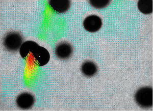
Before the velocity interrogation is performed, the comparatively large bubble shadows are masked and only interrogation areas outside the mask are considered. This is done by first applying a Gaussian and a median filter on the image to blur the small tracer particles, and then the much darker bubble shadows are masked (see figure 2) using a grey value threshold of 110. Velocity fields are generated using a multipass-refinement procedure, with  $3$ refinement steps that result in a final interrogation window size of $32 \times 32$ pixels and $50\,\%$ overlap. Measurements are obtained by mounting a macro-lens (Samyang) with a focal length of $100\ \mathrm {mm}$ and an f-stop of $2.8$. This provides a FOV of $13.9\ \mathrm {mm}\,({H_1}) \times 19.5 \mathrm {mm}\,({H_2})$, with a pixel size of $14.7\ \mathrm {\mu }$m. Since this pixel size is even slightly larger than the seeding particle size, the so-called particle sharpening step (Hessenkemper & Ziegenhein Reference Hessenkemper and Ziegenhein2018) is used, which artificially increases the particle size due to a swelling to the neighbouring pixels. Hence, an effective particle size of approximately $3\text{--}4$ pixels is achieved. In the resulting liquid velocity fields, the spatial resolution $\varDelta$ (PSV grid) is approximately $0.23\ \mathrm {mm}$ ( $d_p/\varDelta \approx 11{\sim}17$, see table 1 for different cases). For more details on the PSV method used in the present measurements, including the whole PIV-like post-processing steps, we refer the readers to Hessenkemper & Ziegenhein (Reference Hessenkemper and Ziegenhein2018).

Figure 2. Instantaneous realization of velocity vector over the FOV in the case SmMore with a detected in-focus bubble (sharp interface) in the middle left. The horizontal/vertical dashed lines are examples, indicating the representative points along the lines where the structure functions were computed.
In figure 2 a typical instantaneous FOV with the bubbles and the resulting liquid velocity vector field are shown for the case SmMore. In this snapshot, while there is only one in-focus bubble (identified by the sharp interface), with strong wake entrainment identified in the velocity vector field, the other bubbles are blurred, i.e. out of focus. Tracer particles at these locations cannot be detected, so that no liquid velocity fields are available there.
To obtain converged high-order statistics, for each case considered  $60\ 000$ velocity fields were recorded with an image pair acquisition rate of $1\ \mathrm {Hz}$. With $60\times 84$ interrogation windows in each velocity field, this yields in total ${\approx}3\times 10^{9}$ data points for each case.
2.2.2. Bubble statistics measurement
The bubble statistics and properties are evaluated with a separate set of measurements. For these measurements, the flow configurations are kept exactly the same with the exception that no tracer particles are added to the flow and that a larger FOV of  $40\ \mathrm {mm} \times 80\ \mathrm {mm}$ (width $\times$ height) than with PSV for the liquid phase is investigated to obtain sufficient bubble statistics. Here, we have evaluated $500$ such image pairs for each case considered.
A machine learning procedure is used to detect and intersect overlapping bubbles in the images (Hessenkemper, Ziegenhein & Lucas Reference Hessenkemper, Starke, Atassi, Ziegenhein and Lucas2022). The underlying neural network uses a U-Net architecture (Ronneberger, Fischer & Brox Reference Ronneberger, Fischer and Brox2015) and is trained to find the intersection boundary of a bubble in front of another bubble. Using these intersections, the bubbles are split and an ellipse is fitted to the contour of each bubble. The ellipse parameters are then used to calculate the volume of an axisymmetric spheroid. Since the gas fraction is comparatively small, the number of overlapping bubbles is also small and up to now unevaluated errors connected to this are estimated to approximately  $5\,\%$. Due to the contamination of the bubbles, deviations from an ellipse due to irregular (wobbling) bubble surfaces are only minor. Example images for the two different bubble sizes with fitted ellipses are given in figure 3 for all the cases. The bubble size is then calculated using the volume-equivalent bubble diameter of a spheroid as $d_p=(d_{maj}^{2}d_{min})^{1/3}$, where $d_{maj}$ and $d_{min}$ are the lengths of the major and minor axes of the fitted ellipse, respectively. For the smaller bubbles, the shape is close to a sphere with a small aspect ratio $\chi =d_{maj}/d_{min}=1.12$ and we obtain $d_p=2.7\ \mathrm {mm}$. In contrast with the larger bubbles, we have $d_p=3.8{\sim}3.9\ \mathrm {mm}$ and $\chi =1.3$. Here, ${\rm \Delta} \rho$ is the density difference between the carrier phase and the dispersed phase and $\sigma$ is the surface tensor coefficient. The range of the bubble Reynolds number, $Re_p$, in our experiments is $500{\sim}900$ based on $d_p$ and the bubble to liquid relative velocity. Note that, although no net liquid flow through a cross-section ( $x_2$– $x_3$ plane) is present (i.e. the bulk velocity of the liquid is zero), for bubble columns, the flow exhibits a large-scale circulation in a time-averaged sense with upward flow in the centre and downward flow close to the walls (Mudde Reference Mudde2005). This results in a non-negligible upward flow in the measurement area of the present PSV (shown later in § 3), so that the relative velocity in the FOV is in general not equal to the bubble terminal rise velocity. Table 1 lists all the relevant parameters for the bubble properties.

Figure 3. Example images of the bubbles with fitted ellipses for an arbitrary instant: (a) case SmLess, (b) case SmMore, (c) case LaLess and (d) case LaMore (figures are cut from a region of the FOV for the gas phase for the corresponding case).
A shallow DoF is used for the measurements conducted to obtain bubble statistics, but it is an order of magnitude larger than that for the liquid velocity measurements due to the different optical system for these two sets of experiments. To measure the bubbles in the  $x_3$-centre region, where the liquid velocity measurements were also taken, the average grey value derivative along the bubble contour is calculated. A threshold for this average grey value derivative is used so that only bubbles in the $x_3$-centre region are considered, and the depth of this $x_3$-centre region is approximately $5\ \mathrm {mm}$. Hence, the evaluated depth for the gas phase is an order of magnitude larger than for the liquid velocity, which is, however, necessary due to the size of the bubbles. The number of bubbles that fall into this region ( $40\ \mathrm {mm} \times 80\ \mathrm {mm} \times 5\ \mathrm {mm}$) is between $2500$ and $5000$ summed up over the considered $500$ image pairs depending on the case being considered, and this corresponds to an average void fraction range of $0.26\,\%$ to $1.31\,\%$ (table 1). The bubble velocity was determined by calculating the distance translated by individual bubble centroids, using a standard particle tracking velocimetry algorithm that matches the closest neighbouring bubble in a small search window in the presumed direction of bubble motion (Bröder & Sommerfeld Reference Bröder and Sommerfeld2007).
3. Basic flow characterization
Before exploring the properties of the flow at different scales, we begin with some basic characteristics of the flow as quantified by single-point statistics of both phases. The instantaneous velocity  $\tilde {\boldsymbol {u}}(\boldsymbol {x},t)$ is decomposed into a ensemble-averaged part $\boldsymbol {U}(\boldsymbol {x},t)$ and a fluctuating part $\boldsymbol {u}(\boldsymbol {x},t)$, with associated components $\tilde {u}_i=U_i+u_i$.
For all the cases investigated, it is observed that the local void fraction (figure 4a), the vertical gas/liquid mean velocity (figure 4b) and the liquid fluctuating velocity profiles (figure 4c,d) in the observation region (FOV of either liquid or gas) of the column are constant to a very good approximation, implying statistical homogeneity of the flow in the observation region. As mentioned earlier, for most cases there is a slight upwards mean flow for the liquid phase in the FOV.

Figure 4. One-point statistics along the horizontal axis of FOV for the four considered cases: (a) gas void fraction, (b) liquid/gas vertical velocity and liquid fluctuating velocity in (c) vertical and (d) horizontal components.
According to figure 4, the root-mean-square value of the vertical velocity fluctuation  $u_1^{rms}$ is significantly larger than the horizontal component $u_2^{rms}$ for each case, indicating the large-scale anisotropy in the flow due to the preferential direction of the bubble motion. The ratio of the vertical to horizontal velocity fluctuation $u_1^{rms}/u_2^{rms}$ is in the range $1.4$ to $1.6$ for the four cases investigated, which is close to the previous studies of Riboux et al. (Reference Riboux, Risso and Legendre2010) and Ma et al. (Reference Ma, Ott, Fröhlich and Bragg2021) for bubbles with sizes in the range $1$ to $3\ \mathrm {mm}$. For both components, we find the velocity fluctuations increase with increasing $\alpha$ – from SmLess to LaMore.
Following Ma et al. (Reference Ma, Ott, Fröhlich and Bragg2021), we define a Reynolds number  $Re_{H_2}\equiv u^{\ast } H_2/\nu$ which indicates the range of scales in the turbulent bubbly flows. Here, $u^{\ast }\equiv \sqrt {(2/3)k_{{FOV}}}$, and $k_{{FOV}}$ is the weighted turbulent kinetic energy (TKE), $k_{{FOV}}=((u_1^{rms})^{2}+2(u_2^{rms})^{2})/2$, assuming axisymmetry of the flow in the FOV about the vertical direction, and averaged over the FOV of the liquid phase. Note that for our experiments the bulk Reynolds number is zero, since there is no averaged net liquid flow when averaged over the entire flow cross-section. Moreover, we are interested in the properties of the fluctuating velocity field, and hence it is more appropriate to consider a Reynolds number based on $u^{\ast }$.
In figure 5 we plot  $Re_{H_2}$ vs large-scale anisotropy ratio $u_1^{rms}/u_2^{rms}$ (averaged over the FOV of liquid). The figure shows that $Re_{H_2}$ increases in the order of SmLess, SmMore, LaLess to LaMore, which corresponds to larger bubbles and higher void fraction. Since the Reynolds number of the flow is usually understood to be related to the range of excited scales of motion in the system, this result implies that in the aforementioned sequence the range of excited scales also increases in the flow, hence, the flow becomes increasingly multiscale. Furthermore, we find that for large scales whose velocities are characterized by $u_1^{rms}$ and $u_2^{rms}$, the smaller bubbles produce more anisotropy in the flow than the larger bubbles, as indicated by a larger ratio of $u_1^{rms}/u_2^{rms}$ for the cases SmLess and SmMore. This is in very close agreement with our previous study based on DNS data of bubble-laden turbulent channel flow driven by a vertical pressure gradient (Ma et al. Reference Ma, Ott, Fröhlich and Bragg2021).

Figure 5. Reynolds number,  $Re_{H_2}$, plotted vs large-scale anisotropy ratio, $u_1^{rms}/u_2^{rms}$.
To quantify the PSV resolution with respect to the Kolmogorov scale  $\eta$, we estimate the mean dissipation $\epsilon$ based on an algebraic relation derived by Ma, Lucas & Bragg (Reference Ma, Lucas and Bragg2020a) for BIT-dominated flows
 \begin{equation} \epsilon=S_k/(1-\alpha) , \end{equation}
where the interfacial term  $S_k$ for the TKE transport equation is adopted from Ma et al. (Reference Ma, Santarelli, Ziegenhein, Lucas and Fröhlich2017) and Ma (Reference Ma2017)
 \begin{equation} S_{k}=\min(0.18Re_{p}^{0.23},1)\boldsymbol{F}_{D}\boldsymbol{\cdot}\boldsymbol{u}_r . \end{equation}
Here,  $\boldsymbol {u_r}$ is the mean slip velocity between the bubble and the liquid, and $\boldsymbol {F}_{D}=(3/4d_p)C_D\alpha \|\boldsymbol {u}_r\|\boldsymbol {u}_r$ is the drag force on the bubbles averaged over the FOV of the liquid. We can then compute the Kolmogorov length scale $\eta \equiv (\nu ^{3}/\epsilon )^{1/4}$, as well the time scale $\tau _\eta \equiv (\nu /\epsilon )^{1/2}$. Both parameters and the ratio of $\varDelta /\eta$ (ranges between $1.8$ and $2.8$) are given in table 2 for all the cases. The current PSV spatial resolution and the size of the liquid FOV are comparable to the recent experimental study of Carter & Coletti (Reference Carter and Coletti2017) on single-phase turbulence using standard PIV (see their small FOV/high resolution measurement).
In figure 6 we plot the PDFs of the liquid velocity fluctuations for both directions, normalized by their standard deviations. Due to the large quantity of velocity fields recorded from the experiment the PDFs are well converged with tails extending to extreme values, with values of the PDF spanning six orders of magnitude, which is much greater than previous experiments for bubbly flows (Riboux et al. Reference Riboux, Risso and Legendre2010; Alméras et al. Reference Alméras, Mathai, Lohse and Sun2017; Lai & Socolofsky Reference Lai and Socolofsky2019). Both the vertical and horizontal velocity PDFs are in good quantitative agreement with the previous experimental studies just mentioned. While PDFs of the horizontal velocity fluctuations are symmetric and non-Gaussian, for the vertical component, the PDFs are strongly positively skewed for all the cases. This positive asymmetry originates from the wake entrainment as visualized in figure 2 for the region directly behind the in-focus bubble, which leads to a larger probability of upward fluctuations. The asymmetry of the PDFs is highest for the case SmLess with the lowest gas void fraction and gradually reduces at larger  $Re_{H_2}$. In our four cases, $Re_{H_2}$ increases with increasing $\alpha$, and a similar trend was also reported in figure 5(a) of Prakash et al. (Reference Prakash, Mercado, van Wijngaarden, Mancilla, Tagawa, Lohse and Sun2016). Furthermore, for the PDF of the horizontal velocity component, SmLess is the furthest from Gaussian, associated with stronger large-scale intermittency than the other cases. In many aspects, those results are very different from those of homogeneous isotropic turbulence for single-phase flows, for which the PDFs of the velocity fluctuations are almost Gaussian (Gotoh, Fukayama & Nakano Reference Gotoh, Fukayama and Nakano2002).

Figure 6. Normalized PDFs of liquid velocity fluctuations: (a) the vertical component and (b) the horizontal component.
4. Turbulence anisotropy quantified using structure functions
While Kolmogorov's theory assumes local isotropy at the small scales of turbulent flows (Kolmogorov Reference Kolmogorov1941, K41 for brevity), many experimental and DNS results reveal persistent anisotropy because the process of a return to isotropy at progressively smaller scales can be very slow (Pumir & Shraiman Reference Pumir and Shraiman1995; Shen & Warhaft Reference Shen and Warhaft2000; Ouellette et al. Reference Ouellette, Xu, Bourgoin and Bodenschatz2006; Carter & Coletti Reference Carter and Coletti2017). The most systematic approach for characterizing anisotropy at different scales is based on the use of irreducible representations of the SO(3) group (Arad, L'vov & Procaccia Reference Arad, L'vov and Procaccia1999; Biferale & Procaccia Reference Biferale and Procaccia2005). However, this method requires information on from the complete three-dimensional flow fields, which is often not available. Due to this practical difficulty, many studies on turbulence anisotropy are based on the velocity structure function tensor, and then characterizing anisotropy based on how this quantity varies in different flow directions. The  $n$th-order structure function is defined as
 \begin{equation} \boldsymbol{D}_n(\boldsymbol{r},t)\equiv\langle {\rm \Delta} \boldsymbol{u}^{n}(\boldsymbol{x},\boldsymbol{r},t) \rangle , \end{equation}
where  ${\rm \Delta} \boldsymbol {u}(\boldsymbol {x},\boldsymbol {r},t)\equiv \boldsymbol {u}(\boldsymbol {x}+\boldsymbol {r},t)-\boldsymbol {u}(\boldsymbol {x},t)$ is the fluid velocity increment, and $\langle \cdot \rangle$ denotes an ensemble average. The calculation of liquid velocity increments in a bubbly flow is, however, delicate, since the liquid velocity is not defined at points occupied by a bubble. To overcome this non-continuous velocity signal challenge, we use the method proposed in Ma et al. (Reference Ma, Santarelli, Ziegenhein, Lucas and Fröhlich2017) – store only liquid velocity data along the horizontal/vertical PSV grid lines whenever the entire line is free from bubbles in the considered FOV (see the two dashed lines in figure 2 for example). Based on the $60\ 000$ velocity fields that were recorded for each case, we were able to extract data along $500\ 000$ to $1\ 500\ 000$ such vertical/horizontal lines, depending on the case. Note that Freund & Ferrante (Reference Freund and Ferrante2019) employed wavelet transforms to handle discontinuities of the velocity field at the bubble interface, and it would be interesting in future work to see how this could be used in analysing experimental data as an alternative to only extracting data along lines free of bubbles.
4.1. Second-order structure function
We first consider the second-order structure function, whose components are
 \begin{equation} D_2^{ij}(\boldsymbol{x},\boldsymbol{r},t)\equiv\langle {\rm \Delta} u_i(\boldsymbol{x},\boldsymbol{r},t){\rm \Delta} u_j(\boldsymbol{x},\boldsymbol{r},t) \rangle . \end{equation}
Hereafter, we suppress the space  $\boldsymbol {x}$ and time $t$ arguments since we are considering a flow which is statistically homogeneous and stationary flows over the FOV. The PSV technique provides access to data associated with separations along two directions, namely, the vertical separation $\boldsymbol {r}=r_1\boldsymbol {e}_1 (r_1\equiv \|\boldsymbol {r}\|)$ and the horizontal separation $\boldsymbol {r}=r_2\boldsymbol {e}_2 (r_2\equiv \|\boldsymbol {r}\|)$. Hence, we are able to compute the four contributions
 $$\begin{gather} D^{L}_2(r_1)=D_2^{11}(r_1) , \end{gather}$$
 $$\begin{gather}D^{L}_2(r_2)=D_2^{22}(r_2) , \end{gather}$$
 $$\begin{gather}D^{T}_2(r_1)=D_2^{22}(r_1) , \end{gather}$$
 $$\begin{gather}D^{T}_2(r_2)=D_2^{11}(r_2) , \end{gather}$$
based on the Cartesian coordinate system depicted in figure 1. For an incompressible and isotropic flow, the following relation holds for the transverse structure function:
 \begin{equation} D^{T}_{2,iso}(r_\gamma)=D^{L}_{2}(r_\gamma)+\frac{r_\gamma}{2} \frac{\partial}{\partial{r_\gamma}}D^{L}_{2}(r_\gamma) , \end{equation}
where no summation over  $\gamma$ is implied.
Figure 7 shows all the measured components of the second-order structure function, as well as  $D^{T}_{2,iso}(r_\gamma )$ obtained from (4.7) for the representative case SmLess in figure 7(a,d). The results show that the values of the structure functions increase in the order SmLess, SmMore, LaLess and LaMore, which corresponds to increasing $Re_{H_2}$, gas void fraction and/or bubble Reynolds number. This relationship holds for all of the components computed and across all scales. A similar trend was also reported for all three diagonal components of the second-order structure function based on separations in the spanwise direction of a bubble-laden turbulent channel flow in our recent study (Ma et al. Reference Ma, Ott, Fröhlich and Bragg2021). The second-order structure function is also related to the energy spectrum, which is often considered in analysing bubble laden flows. In figure 8 we plot the energy spectra corresponding to $u_1$ for horizontal wavenumbers, and the results show the behaviour $E_{11}\sim \kappa ^{-3}$ for all the cases, as observed in previous studies which was discussed in § 1. We also note that the $-3$ scaling spans wavelengths in the approximate range $1\times 10^{-3}$ to $5\times 10^{-3}\ {\rm m}$. If the bubble wake is approximately statistically axisymmetric due to the bubble shape, and if the $-3$ range is associated with the bubble wake, then since the upper value $5\times 10^{-3}\ {\rm m}$ is ten times smaller than the depth of the column, the wake should be only weakly affected by the walls of the column in the $x_3$ direction, for bubbles in the FOV. However, this is only an estimate, and it is possible that the finite column depth relative to the bubble size could play some role in restricting the bubble wake development, a point for exploration in future work.

Figure 7. Measured second-order transverse (a,d) and longitudinal (b,c) structure functions, with separations along the horizontal (a,b) and the vertical (c,d) directions. Note that  $D^{T}_{2,iso}(r_i)$ calculated with (4.7) is shown for SmLess in (a,d).

Figure 8. One-dimensional energy spectra of the vertical component of the fluctuating liquid velocity, where the wavevector is in the horizontal direction. The two vertical dashed lines denote the wavelength  $\kappa ^{-1}=d_p$ for smaller and larger bubbles, respectively.
At the large scales of a homogeneous flow both  $(1/2)D^{11}_2(r_\gamma )/\langle u_1u_1\rangle$ and $(1/2)D^{22}_2(r_\gamma )/\langle u_2u_2\rangle$ approach unity. Our data for these normalized quantities are shown in figure 20 in Appendix A and reveal that, along the separation $r_2$, the quantities converge to unity when $r_2\rightarrow H_2$. However, while $(1/2)D^{22}_2(r_1\rightarrow H_1)/\langle u_2u_2\rangle$ approaches unity, $(1/2)D^{11}_2(r_1\rightarrow H_1)/\langle u_1u_1\rangle \approx 0.8$ for all the cases. This implies that the FOV is not large enough in the vertical direction to resolve the integral length scale of the flow in this direction, while it is for the horizontal direction. However, this may be simply due to the fact that $H_1< H_2$ for the FOV.
For the SmLess case, departures from  $D^{11}_2(r_2)=D^{11,iso}_2(r_2)$ are larger at the large scales, reflecting the large-scale anisotropy characterized by e.g. $u^{{rms}}_1/u^{{rms}}_2$ in table 2. At for smallest values of $r_2$, $D^{11}_2(r_2)\approx D^{11,iso}_2(r_2)$. However, for separations along the vertical direction there are strong departures from $D^{22}_2(r_1)=D^{22,iso}_2(r_1)$ at all scales (figure 7d). We obtained similar results (not shown) for the other three cases. Interestingly, such behaviour was also observed in Carter & Coletti (Reference Carter and Coletti2017) for single-phase turbulence generated by jet stirring (with zero mean flow) at a similar range of $u^{{rms}}_1/u^{{rms}}_2$.
For the second-order structure functions, one of other ways to quantify anisotropy is by the ratios of components such as  $D^{L}_2(r_1)/D^{L}_2(r_2)$ and $D^{T}_2(r_2)/D^{T}_2(r_1)$, which would be equal to unity for an isotropic flow. The results in figure 9 show that both ratios monotonically decrease for decreasing separation. While the ratio of the longitudinal structure functions is very close to unity at small scales, the ratio of transverse structure functions departs more strongly from unity. By comparing the different cases, the results indicate that the smaller bubbles generate stronger anisotropy in the flow than the larger bubbles across the scales, which is in agreement with the DNS results in Ma et al. (Reference Ma, Ott, Fröhlich and Bragg2021) and also the results of large-scale anisotropy in § 3.

Figure 9. Ratio of longitudinal (a) and transverse (b) structure functions in different separation directions for all the cases. In (a,b) the horizontal lines indicate the value of unity and the two vertical dashed lines show  $r=d_p$ for smaller and larger bubbles, respectively.
In general, the differing behaviour of the second-order structure function in the longitudinal and transverse directions shows that both need to be considered in order to fully consider the turbulence anisotropy across scales. This conclusion based on our bubble-laden flow is in agreement with that of Carter & Coletti (Reference Carter and Coletti2017) for single-phase turbulence.
4.2. High-order structure function
Next, we consider measures of the anisotropy based on even-order structure functions up to order twelve by considering the ratios  $D^{L}_n(r_1)/D^{L}_n(r_2)$ and $D^{T}_n(r_2)/D^{T}_n(r_1)$ which would be equal to unity for an isotropic flow. Using higher-order structure functions allows for a characterization of how anisotropic the large fluctuations in the system are. The results in figures 10 and 11 show that the data are statistically well converged up to order 8. We also performed a convergence check by comparing the higher-order moments computed only using half of the data, and using the full data. The results showed that for structure functions up to eighth order the two results were almost identical, indicating that our results are statistically converged due to the very large number of data points obtained in the experiments. For orders 10 and 12, the results are not fully converged. However, although there is considerable noise, the general trend of the results seems clear. The results show that the ratios $D^{L}_n(r_1)/D^{L}_n(r_2)$ and $D^{T}_n(r_2)/D^{T}_n(r_1)$ deviate increasingly strongly from unity as $n$ is increased, with the results for $n\geq 6$ reaching values very far from unity across most of the flow scales. This shows that extreme fluctuations in the flow are more anisotropic than the ‘typical’ fluctuations characterized by the $n=2$ results. Similar behaviour has also been observed for single-phase turbulence, showing that higher-order moments are the most anisotropic (Kurien & Sreenivasan Reference Kurien and Sreenivasan2000; Warhaft & Shen Reference Warhaft and Shen2002). For the longitudinal directions, the results show that, just as for the $n=2$ results, the cases with smaller bubbles exhibit greater anisotropy than those with larger bubbles. However, for the transverse direction the LaLess case is by far the most anisotropic. We are not aware of a good explanation for this differing dependence of the longitudinal and transverse anisotropy on the properties of the bubbles.

Figure 10. Ratio of  $n$th-even-order longitudinal structure functions in different separation directions for all the cases ( $n=2, 4, 6, 8, 10, 12$). The grey horizontal line in each plot indicates the isotropic value of unity. Note that (a) presents the same value as figure 9(a), just with a different label of $y$-axis.

Figure 11. Ratio of  $n$th-even-order transverse structure functions in different separation directions for all the cases ( $n=2, 4, 6, 8, 10, 12$). Note that (a) presents the same value as figure 9(b), just with a different label of $y$-axis.
5. Energy transfer
We now turn to considering the mean energy transfer in the flow, by analysing the third-order structure function as well as the related inter-scale energy transfer term (Hill Reference Hill2001; Alexakis & Biferale Reference Alexakis and Biferale2018)
 \begin{equation} \mathcal{F}(\boldsymbol{r})=\left.\sum_{\gamma=1}^{3}\mathcal{F}_\gamma(\boldsymbol{r})\equiv \sum_{\gamma=1}^{3} \sum_{\gamma=1}^{3}\frac{\partial}{\partial \xi_\gamma}D^{\gamma ii}_3(\boldsymbol{\xi})\right\vert_{\boldsymbol{\xi}=\boldsymbol{r}},\end{equation}
that appears in the Kármán–Howarth-type equation governing  $D^{ii}_2(\boldsymbol {r})$, where $D^{\gamma ii}_3(\boldsymbol {r})\equiv \langle {\rm \Delta} {u_\gamma }(\boldsymbol {r}) {\rm \Delta} u_i(\boldsymbol {r}){\rm \Delta} u_i(\boldsymbol {r})\rangle$. Note that the divergence term in (5.1) has been written using the variable $\boldsymbol {\xi }$ to emphasize that this term involves the divergence evaluated at $\boldsymbol {r}$.
The sign of  $\mathcal {F}$ indicates the direction of the nonlinear energy transfer between the scales of the flow, and in three-dimensional single-phase turbulence, we have $\mathcal {F}<0$ in the inertial and dissipation ranges, corresponding to a downscale transfer of energy from large to small scales on average. With our two-dimensional PSV data we are not able to construct the full quantity $\mathcal {F}$, however, we are able to consider some of the contributions $\mathcal {F}_\gamma$.
In figure 12 we plot the components  $\mathcal {F}_1(r_1)=d(D^{111}_3+D^{122}_3)/dr_1$ and $\mathcal {F}_2(r_2)=d(D^{222}_3+D^{211}_3)/dr_2$. The peaks in the magnitudes of both $\mathcal {F}_1$ and $\mathcal {F}_2$ increase in the sequence SmLess, SmMore, LaLess and LaMore, which corresponds to higher $Re_{H_2}$, $\alpha _p$ and/or $Re_p$. This is in part simply due to the fact that the kinetic energy in the flow increases in this sequence also, and with more kinetic energy at the large scales, there is more available to be passed downscale. Concerning $\mathcal {F}_1$, the results show that at scales $r>O(d_p)$, $\mathcal {F}_1<0$ corresponding to energy moving downscale, while at scales $r< O(d_p)$, $\mathcal {F}_1>0$, corresponding to energy moving upscale. In contrast to $\mathcal {F}_1$, the contribution $\mathcal {F}_2$ shows an opposite trend, with $\mathcal {F}_2<0$ for at smaller scales indicating a downscale energy transfer. The magnitude of $\mathcal {F}_2$ is, however, in general much larger than $\mathcal {F}_1$, implying a higher energy transfer rate in the horizontal direction of the flow. At the low Reynolds number of the flow, there is no inertial range over which either $\mathcal {F}_1$ or $\mathcal {F}_2$ are constant, indicating that the nonlinear energy transfer is not in the form of a constant flux cascade.

Figure 12. Contribution  $\mathcal {F}_1$ (a) and $\mathcal {F}_2$ (b) to the nonlinear energy transfer term for all the cases. In (a,b) the two vertical dashed lines show $r=d_p$ for smaller and larger bubbles, respectively.
Our previous study (Ma et al. Reference Ma, Ott, Fröhlich and Bragg2021) explored bubble-laden turbulent channel flows and also observed that there is a downscale energy transfer for  $\mathcal {F}_3(r_3)$ (where in that paper the 3 direction corresponded to the spanwise direction of the channel flow). However, in that study we could not compute either $\mathcal {F}_1$ (streamwise) or $\mathcal {F}_2$ (wall normal) due to the one-dimensional dataset being used. Although the type of flow presently under consideration is considerably different from a pressure driven bubble-laden turbulent channel flow, the results nevertheless indicate that the nonlinear energy transfer behaviour may be very different in the different directions of the flow.
These results therefore show that the direction of the energy flux can differ from one direction to another, with  $\mathcal {F}_1$ revealing an upscale energy transfer at smaller scales, while $\mathcal {F}_2$ reveals the opposite. Therefore, although the total energy transfer may be downscale in bubbly turbulent flows (Pandey et al. Reference Pandey, Ramadugu and Perlekar2020), some directions of the flow can exhibit an upscale transfer.
The energy transfer term  $\mathcal {F}$ depends on the third-order structure function, and its behaviour may be further understood by considering the associated skewness of the velocity increments. Figure 13 shows $D^{L}_3/(D^{L}_2)^{3/2}$ (the skewness of the longitudinal velocity increment) for the two separations $r_1$ and $r_2$. The results show that when $D^{L}_3(r_2)$ is plotted in this normalized form, the results for all of the cases almost collapse, and $D^{L}_3(r_2)/(D^{L}_2(r_2))^{3/2}$ is not far from the value $-0.4$ that occurs for single-phase isotropic turbulence (Davidson Reference Davidson2015) for $r\rightarrow 0$. The negative longitudinal skewness along the separation perpendicular to the bubble motion direction was also found in Ma et al. (Reference Ma, Ott, Fröhlich and Bragg2021) for some of the bubble-laden cases considered, however, for other cases this skewness was actually positive. This is very different from our results where all the cases considered have very similar negative values of the skewness. It is not clear as to whether this is due to the different kinds of flows being studied here and in Ma et al. (Reference Ma, Ott, Fröhlich and Bragg2021), or perhaps also because of differences in the parameter space of the bubbles being explored. For vertical separations $r_1$, $D^{L}_3(r_1)/(D^{L}_2(r_1))^{3/2}$ also almost collapses for all the cases but is positive at the small scales with a similar magnitude $\approx 0.4$ to the results for $D^{L}_3(r_2)/(D^{L}_2(r_2))^{3/2}$. This again indicates strong anisotropy for the odd-order structure functions, just as for the even-order structure functions discussed in § 4.

Figure 13. Normalized third-order longitudinal structure functions (skewness), with separations along the horizontal (a) and the vertical (b) directions. The horizontal lines in (a,b) indicate the value of zero.
Similar plots are obtained for the transverse structure functions  $D^{T}_3(r_2)$ and $D^{T}_3(r_1)$. The corresponding skewness values were found to be close to zero in both separations directions for all the cases (not shown here).
6. Extreme fluctuations in the flow
Having considered the flow anisotropy and nonlinear energy transfer, we now turn to consider the extreme fluctuations in the flow. Single-phase turbulence at high Reynolds number exhibits fluctuations in space and time of its small-scale quantities that are orders of magnitude larger than the average values, a phenomenon referred to as small-scale intermittency (Frisch Reference Frisch1995; Sreenivasan & Antonia Reference Sreenivasan and Antonia1997). Such extreme fluctuations are critical for many processes in both nature and engineering (Sapsis Reference Sapsis2021), and their investigation continues to be an area of active research (Yeung, Zhai & Sreenivasan Reference Yeung, Zhai and Sreenivasan2015; Buaria et al. Reference Buaria, Pumir, Bodenschatz and Yeung2019). However, very few studies have explored the topic of intermittency in bubble-laden turbulent flows (see the related works introduced in § 1). In what follows, we focus on extreme fluctuations of the velocity increments  ${\rm \Delta} \boldsymbol {u}$ in the bubble-laden flow we are considering.
6.1. Probability density functions
Figure 14 shows the instantaneous velocity increments  ${\rm \Delta} u_i(r_2=\varDelta )$, normalized by their standard deviations $\sigma _{{\rm \Delta} u_i}$ along a line (without bubbles) in the direction of $x_2$ within the FOV. The plots reveal intermittent fluctuations of ${\rm \Delta} u_i(r_2=\varDelta )$, with relatively small regions where ${\rm \Delta} u_i(r_2=\varDelta )/\sigma _{{\rm \Delta} u_i}$ takes on large values, between which there are relatively small fluctuations of ${\rm \Delta} u_i(r_2=\varDelta )/\sigma _{{\rm \Delta} u_i}$. We will return later to considering how these intermittent large fluctuations of ${\rm \Delta} u_i(r_2=\varDelta )/\sigma _{{\rm \Delta} u_i}$ are associated with the bubble wakes in the flow.

Figure 14. Instantaneous velocity increments normalized by standard deviations: (a)  ${\rm \Delta} u_1(r_2=\varDelta )/\sigma _{{\rm \Delta} u_1}$ and (b) ${\rm \Delta} u_2(r_2=\varDelta )/\sigma _{{\rm \Delta} u_2}$, along an arbitrary horizontal line for an instant, when the line is free of bubbles for each considered case. In (a,b) the curves for SmMore, LaLess and LaMore are shifted upward by $7, 14$ and $21$, respectively, for a better visual representation.
To statistically quantify the extreme events in the flow, the PDFs of the velocity increments can be considered, and these are shown in figure 15, normalized by the standard deviation, for separations equal to one PSV grid  $(r=\varDelta )$. All of the results in figure 15 show that the velocity increments have strongly non-Gaussian PDFs, consistent with the observations based on figure 14. While the PDFs of the transverse velocity increments in panels (a,d) are almost symmetric, the PDFs of the longitudinal velocity increment are negatively skewed for horizontal separations $r_2$, panel (b), and positively skewed for vertical separations $r_1$, panel (c), consistent with the skewness results in figure 13. The results also show that the PDFs become increasingly non-Gaussian in the order of LaMore, LaLess, SmMore, SmLess, which corresponds to the order of decreasing Reynolds number. Therefore, surprisingly, while non-Gaussianity of the PDFs of the velocity increments becomes stronger as Reynolds number is increased in single-phase turbulence (Frisch Reference Frisch1995), the opposite occurs for the bubble-laden turbulent flow considered here.

Figure 15. Normalized PDFs of the transverse (a,d) and longitudinal (b,c) velocity increments, with the separation  $r=\varDelta$ along the horizontal (a,b) and the vertical (c,d) directions for all four cases.
In turbulent flows, intermittency is characterized not simply by non-Gaussianity of the small-scale flow quantities, but also by the non-Gaussianity depending on scale (as well as Reynolds number) (Frisch Reference Frisch1995). To consider intermittency in the flow we therefore consider how the normalized PDFs of the velocity increments change with scale. Figure 16 shows the PDFs of the transverse (a,d) and longitudinal (b,c) velocity increments for various separation distances  $r_\gamma =\varDelta, 10\varDelta,20\varDelta, 40\varDelta, H_\gamma$ and for the representative case SmMore. The general behaviour is very similar to that observed for single-phase turbulence (Ishihara, Gotoh & Kaneda Reference Ishihara, Gotoh and Kaneda2009): as the scale is decreased, the PDFs of both the transverse (a,d) and longitudinal (b,c) velocity increments deviate more and more from a Gaussian distribution with the tails becoming increasingly heavy, and the PDFs becoming increasingly peaked. For the PDFs of longitudinal velocity increments are negatively skewed for ${\rm \Delta} u_2(r_2)$ and positively skewed for ${\rm \Delta} u_1(r_1)$, but the skewness becomes progressively weaker as the scale increases, and for the largest scale captured in the FOV, i.e. $r_\gamma =H_\gamma$, we find almost symmetric PDFs.

Figure 16. Normalized PDFs of the transverse (a,d) and longitudinal (b,c) velocity increments in the case SmMore for various separation distances  $r_i=\varDelta, 10\varDelta,20\varDelta, 40\varDelta, H_i$, where $\varDelta$ is one PSV grid. (a,b) Separations along the horizontal direction and (c,d) separations along the vertical direction.
We note that, while the PDFs of the velocity increments should asymptote to the single-point PDFs of the velocity in the limit  $r\rightarrow \infty$, our data for the PDF of ${\rm \Delta} u_1(r_\gamma =H_\gamma )$ are very different (compare the left tails of the PDFs) from single-point PDF of $u_1$ shown in figure 6(a). This is probably simply due to the fact that, as already noted earlier, the size of the FOV is not large enough for this asymptotic regime to be observed. The aforementioned PDFs are, however, so different that the flow behaviour must undergo an interesting transition where negative fluctuations of the vertical velocity begin to be suppressed (but not positive fluctuations) as the scale continues to be increased. This point will be explored in a future work by employing a larger FOV to observe this asymptotic regime.
6.2. Flatness of velocity increment
The intermittency and non-Gaussianity can be quantified using the flatness measures defined as  $D^{T}_4(r_\gamma )/(D^{T}_2(r_\gamma ))^{2}$ (figure 17a,d) and $D^{L}_4(r_\gamma )/(D^{L}_2(r_\gamma ))^{2}$ (figure 17b,c). The first observation from the results in figure 17 is that all four bubble-laden cases show a rather similar behaviour as $r$ increases, slowly reducing from values of up to 40 towards the Gaussian value of 3. However, there is still considerable deviation from 3 even at the largest scale $r_\gamma /H_\gamma =1$, consistent with the PDF results for ${\rm \Delta} \boldsymbol {u}(r_\gamma =H_\gamma )$ in figure 16. We also find that, for both the transverse or longitudinal flatness measures and along either separation direction, the flatness is largest for the case with smaller $Re_{H_2}$, reflecting the same trend as the PDFs of the velocity increments at the single scale $\varDelta$ (figure 15). The values and behaviour of the flatness are similar to those observed in Ma et al. (Reference Ma, Ott, Fröhlich and Bragg2021) for the three bubble-laden cases with $\alpha _p=2.14\,\%$, although for the present flow the flatness values are larger than those in Ma et al. (Reference Ma, Ott, Fröhlich and Bragg2021). For separations $r_2$, the transverse flatness values are larger than the longitudinal ones, similar to that observed in isotropic turbulence (Li & Meneveau Reference Li and Meneveau2005; Ishihara et al. Reference Ishihara, Gotoh and Kaneda2009). In contrast, for separations $r_1$, the transverse flatness values are slightly smaller than the longitudinal ones.

Figure 17. Normalized fourth-order transverse (a,d) and longitudinal (b,c) structure functions, corresponding to the flatness of the velocity increments. The horizontal lines in (a–d) indicate the Gaussian value of  $3$ for the flatness.
6.3. Flow structures associated with extreme fluctuations
We now use flow visualization to understand which regions of the flow are associated with the extreme velocity increments. Figure 18(c,d) gives two examples of such flow visualization extracted from a randomly chosen (but representative) FOV result for  ${\rm \Delta} u_1(r_2=\varDelta )/\sigma _{u_1}$ for the cases SmMore and LaMore, respectively. Each grid in the figure corresponds to an interrogation window of the present PSV. For convenience, we also plot in (a,b) the corresponding original velocity vector fields and denote in each case the in-focus bubbles. The images show that for both cases the regions where the velocity increment takes on extreme values are located in the outer-most region of the individual bubble wakes, while the fluctuations inside the wakes are relatively weak (see c,d). At a result of this it appears that the small-scale intermittency in the present flow already characterized is quite different from the small-scale intermittency that occurs in single-phase turbulence that arises due to nonlinear self-amplification of the velocity gradients (Tsinober Reference Tsinober2001; Li & Meneveau Reference Li and Meneveau2005; Buaria et al. Reference Buaria, Pumir, Bodenschatz and Yeung2019; Buaria, Bodenschatz & Pumir Reference Buaria, Bodenschatz and Pumir2020). In particular, the intermittency in the present flow is more similar to what is often called external intermittency (Townsend Reference Townsend1949), which arises near the interface between two regions of the flow with significantly differing behaviour, e.g. such as at the turbulent/non-turbulent interface in turbulent jets (da Silva et al. Reference da Silva, Hunt, Eames and Westerweel2014; Gauding et al. Reference Gauding, Bode, Brahami, Varea and Danaila2021). In the bubble-laden flow we are considering, the intermittency arises at the interface between the edge of the bubble wake and the surrounding relatively quiescent flow.

Figure 18. Snapshot of the original velocity vector (a,b) and the intensity distributions of normalized velocity increment  ${\rm \Delta} u_1(r_2=\varDelta )/\sigma _{{\rm \Delta} u_1}$ (c,d). Here, (a,c) are from the same instant based on the SmMore case and (b,d) are from the same instant based on the LaMore case. The in-focus bubbles are denoted in (a,b).
One further observation on figure 18(c,d) is that the extreme values are larger for the smaller bubble wakes than the larger bubble wakes (note the different legend scales in c,d). This point is made clearer in figure 19(a,b) where instead  $|{\rm \Delta} u_1(r_2=\varDelta ) |\geq 8\sigma _{{\rm \Delta} u_1}$ is plotted. Looking at the in-focus bubble on the right-hand side for both cases (where a more complete wake structure is visible than for the left in-focus bubble), we find that the regions of extreme values are larger for the SmMore case. By increasing the threshold to $|{\rm \Delta} u_1(r_2=\varDelta ) |\geq 16\sigma _{{\rm \Delta} u_1}$ (figure 19c,d), we see that there are still some locations with extreme values satisfying this threshold for the SmMore, while there are none for the LaMore case. Although this observation is only for one snapshot, we have conducted the same analysis for many different snapshots and virtually all of them show the same behaviour. These observations are consistent with the PDF results in figure 15 that show that cases with smaller bubbles (lower $Re_{H_2}$) have heavier tails than the cases with larger bubbles (higher $Re_{H_2}$).

Figure 19. Snapshots indicating the regions with extreme values, where  $|{\rm \Delta} u_1(r_2=\varDelta ) |\geq 8\sigma _{{\rm \Delta} u_1}$ (a,b) and $|{\rm \Delta} u_1(r_2=\varDelta ) |\geq 16\sigma _{{\rm \Delta} u_1}$ (c,d) highlighted in red. Panels (a,c) are from the same instant from SmMore and (b,d) are from the same instant from LaMore. The in-focus bubbles are denoted in each panel.
An explanation for why the intermittency is largest for the cases with smaller bubbles and lower volume fractions was given in Ma et al. (Reference Ma, Ott, Fröhlich and Bragg2021). When the volume fraction is not too large (but still large enough for the bubbles to make a statistically significant contribution to the flow properties), there are relatively few regions in the flow where turbulence is produced due to the bubble wakes, meaning that turbulence in the flow is very patchy and therefore intermittent. As the volume fraction increases, the regions of the flow influenced by the bubble wakes becomes less rare, and hence intermittency in the flow reduces. This then explains why the SmLess case is the most intermittent, and the LaMore case the least intermittent. Moreover, since the flow we are considering has no background turbulence (i.e. the only turbulence in the flow is the result of the bubble wakes), then this may explain why the intermittency we see is higher than that in Ma et al. (Reference Ma, Ott, Fröhlich and Bragg2021) where the flow considered had background turbulence, so that turbulent activity in the flow was not restricted to regions close to the bubbles.
7. Conclusions
In this paper we have presented an analysis of the multiscale properties of a bubble-laden turbulent flow, based on experimental data of a flow in a vertical column with bubble swarms rising in water. The experiment takes advantage of a recently developed PSV technique for particle/bubble flows and provides the first comprehensive dataset for computing multipoint measurements (without having to invoke Taylor's hypothesis, in contrast to, e.g. Rensen et al. Reference Rensen, Luther and Lohse2005) of flows laden with finite-sized bubbles. By acquiring a very large number of snapshots of the velocity field we are able to compute structure functions of up to twelfth order, and PDFs that resolve the heavy tails associated with extreme fluctuations in the flow.
The results show that the level of anisotropy in the flow produced by the rising bubbles is strong in general, and not negligible at any scale in the flow. Moreover, the results show that (i) the differing behaviour of the second-order longitudinal and transverse structure functions when measured for separations in different directions shows that both velocity components and separation directions of the two-dimensional data need to be considered in order to fully characterize the anisotropy of the flow; (ii) the bubble size and void fraction are both important parameters determining the amount of anisotropy in the flow; (iii) higher-order structure functions reveal greater anisotropy across the scales of the flow, such that extreme fluctuations in the flow are the most anisotropic. Since the PSV measurements capture two-dimensional data, we were able to consider the energy transfer between scales for two separation directions in the flow. The results revealed a downscale energy transfer on average for horizontal separations, but an upscale energy transfer on average in the vertical direction. However, the horizontal energy transfer was much stronger than that in the vertical direction.
We also investigated extreme events in the flow by considering the normalized PDFs of the velocity increments in the flow. The results showed that the probability of extreme fluctuations increases with decreasing scale, just as in single-phase turbulence. However, the results also showed that for a given scale the probability of extreme events decreased with increasing Reynolds number, contrary to what occurs in single-phase turbulence. To explore the origin of these extreme fluctuations in the bubble-laden flows, we visualized regions of extreme small-scale velocity increments in the FOV and observed that they are typically located at the boundary of the wakes produced by the bubbles. For the cases with smaller bubbles and lower void fractions, vast regions outside of the bubbles wakes exhibit weak fluctuations, and so this combined with the extreme fluctuations at the bubble wake boundaries leads to strong intermittency. For larger bubbles which produce larger flow Reynolds numbers, and with larger void fractions, the wake regions become less rare in the flow and hence the flow is less intermittent than the former case, even though the Reynolds number is higher. Furthermore, the extreme values were also observed to reach larger values (compared with the standard deviation) for the smaller bubbles, which again causes the smaller bubble cases to exhibit greater intermittency than the larger bubble cases, in addition to the effect arising from the fraction of the flow modified by the bubble wakes.
Finally, it is worth pointing out two limitations with the present PSV data. First, the FOV is not large enough to resolve the integral length scales of the flow, and therefore, as discussed in § 6.1, we were not able to fully resolve the transition in the properties of the bubble-laden flow as the scale approaches the integral length scale. Second, the bubbles considered here all have approximately fixed shape, mimicking in nature small bubbles in a contaminated flow. We are currently performing new experiments with deformable bubbles and differing FOVs in order to address these two points and will report the results in future work.
Acknowledgements
The authors would like to acknowledge T. Ziegenhein for providing some routines for calculating bubble statistics. We also thank R. Franz and U. Hampel for providing the high-speed camera used in the present study.
Funding
T.M. acknowledges funding by Deutsche Forschungsgemeinschaft (DFG, German Research Foundation) under Grants MA 8408/1-1 and MA 8408/2-1.
Data availability
The data that support the findings of this study are available from the first author T.M. on request.
Declaration of interests
The authors report no conflict of interest.
Appendix. Normalized second-order structure functions
Figure 20 shows the second-order structure functions normalized by the Reynolds stresses  $0.5D^{\gamma \gamma }_2/\langle u_\gamma u_\gamma \rangle$. As discussed in the main text, this quantity should approach unity for separations larger than the integral length scale in a homogeneous flow. The fact that the quantities do not approach unity in the experiments for some of the components/choices of $r_\gamma$ indicates that the FOV is smaller than the associated spatial correlation length scale of the flow.

Figure 20. Normalized second-order structure functions, with separations along the horizontal (a,b) and the vertical (c,d) directions. The horizontal lines indicate the value of unity.


 Open access