


1. Introduction
Flows around cylindrical engineering structures are ubiquitous and understanding their stability characteristics is important. For example, in urban settings, understanding of the flow stability past square-shaped buildings is essential for maintaining structural integrity and minimising wind-induced vibrations (Wijesooriya et al. Reference Wijesooriya, Mohotti, Lee and Mendis2023). Likewise, vortex-induced motions in offshore structures such as semi-submersible platforms, driven by vortex shedding and wake dynamics, can lead to pronounced transverse and yaw oscillations that amplify structural responses (Gonçalves et al. Reference Gonçalves, Rosetti, Fujarra and Oliveira2012). Stability analysis of these flows can provide critical insights and help with mitigating risks posed by oscillatory phenomena.
Often, these cylindrical structures are arranged in side-by-side configurations, resembling two-dimensional flows around adjacent square cylinders. This arrangement exhibits a rich tapestry of flow patterns. For example, at Reynolds number $4.7 \times 10^4$
, Alam, Zhou & Wang (Reference Alam, Zhou and Wang2011) identified four regimes (single-body, two-frequency, transition and coupled vortex street) depending on the gap ratio. Ma et al. (Reference Ma, Kang, Lim, Wu and Tutty2017) considered lower
$4.7 \times 10^4$
, Alam, Zhou & Wang (Reference Alam, Zhou and Wang2011) identified four regimes (single-body, two-frequency, transition and coupled vortex street) depending on the gap ratio. Ma et al. (Reference Ma, Kang, Lim, Wu and Tutty2017) considered lower $\textit{Re}$
numbers (between 16 and 200) and gap ratios
$\textit{Re}$
numbers (between 16 and 200) and gap ratios $0{-}10D$
(where
$0{-}10D$
(where $D$
is the edge length of the square cylinders) and identified nine flow regimes. For a range of gap ratios (that depends on the Reynolds number), the vortex streets behind the two cylinders are asymmetric causing the jet emanating from the gap to flap up and down. This behaviour is also well documented for circular cylinder flows and is known as ‘flip-flopping’ or ‘jet switching’ (Kim & Durbin Reference Kim and Durbin1988; Moretti Reference Moretti1993). As the gap increases, the system transitions to synchronised, symmetric or anti-symmetric vortex shedding regimes (see Rao, Ni & Liu Reference Rao, Ni and Liu2008; Ma et al. Reference Ma, Kang, Lim, Wu and Tutty2017). High-fidelity simulations have captured these intricate wake interference patterns (Zhou et al. Reference Zhou, Nagata, Sakai and Watanabe2019, Reference Zhou, Nagata, Sakai, Watanabe, Ito and Hayase2020). Bistable behaviour between distinct vortex-shedding states has been reported in coupled side-by-side Kármán wakes (Ren et al. Reference Ren, Cheng, Xiong, Tong and Chen2021). In-phase, anti-phase and conditional flip-flop states may coexist over transitional ranges of gap ratio and Reynolds number, with the realised state depending sensitively on the initial conditions.
$D$
is the edge length of the square cylinders) and identified nine flow regimes. For a range of gap ratios (that depends on the Reynolds number), the vortex streets behind the two cylinders are asymmetric causing the jet emanating from the gap to flap up and down. This behaviour is also well documented for circular cylinder flows and is known as ‘flip-flopping’ or ‘jet switching’ (Kim & Durbin Reference Kim and Durbin1988; Moretti Reference Moretti1993). As the gap increases, the system transitions to synchronised, symmetric or anti-symmetric vortex shedding regimes (see Rao, Ni & Liu Reference Rao, Ni and Liu2008; Ma et al. Reference Ma, Kang, Lim, Wu and Tutty2017). High-fidelity simulations have captured these intricate wake interference patterns (Zhou et al. Reference Zhou, Nagata, Sakai and Watanabe2019, Reference Zhou, Nagata, Sakai, Watanabe, Ito and Hayase2020). Bistable behaviour between distinct vortex-shedding states has been reported in coupled side-by-side Kármán wakes (Ren et al. Reference Ren, Cheng, Xiong, Tong and Chen2021). In-phase, anti-phase and conditional flip-flop states may coexist over transitional ranges of gap ratio and Reynolds number, with the realised state depending sensitively on the initial conditions.
Global linear stability analysis (GLSA) offers a natural starting point for understanding the origin of some of these patterns. At its simplest form, GLSA considers a given steady base flow and investigates how small disturbances evolve when superimposed on the base flow (Schmid Reference Schmid2007; Theofilis Reference Theofilis2011). This involves the solution of an eigenvalue problem which is solved iteratively using Krylov subspace methods (Edwards et al. Reference Edwards, Tuckerman, Friesner and Sorensen1994). If the perturbations grow exponentially in time, then a primary instability has been detected. The primary instability of the flow past a square cylinder was considered by Yoon, Yang & Choi (Reference Yoon, Yang and Choi2010), Park & Yang (Reference Park and Yang2016), Jiang, Cheng & An (Reference Jiang, Cheng and An2018) and Chiarini, Quadrio & Auteri (Reference Chiarini, Quadrio and Auteri2021). It was found that its onset is similar to that of a circular cylinder with the flow undergoing a Hopf bifurcation. The most recent GLSA of Chiarini et al. (Reference Chiarini, Quadrio and Auteri2021) reports a critical $\textit{Re}_c=44.56$
, which is slightly smaller than the
$\textit{Re}_c=44.56$
, which is slightly smaller than the $\textit{Re}_c=46.6$
of a circular cylinder. Mizushima & Ino (Reference Mizushima and Ino2008) employed GLSA to the symmetric mean flow past a pair of side-by-side circular cylinders.
$\textit{Re}_c=46.6$
of a circular cylinder. Mizushima & Ino (Reference Mizushima and Ino2008) employed GLSA to the symmetric mean flow past a pair of side-by-side circular cylinders.
For $\textit{Re}\gt \textit{Re}_c$
, the flow becomes periodic and, at a certain
$\textit{Re}\gt \textit{Re}_c$
, the flow becomes periodic and, at a certain $\textit{Re}$
, a secondary instability may develop. This is captured by linearising around the two-dimensional periodic base flow and evaluating the evolution of two- or three-dimensional perturbations superimposed on this base flow; this is known as Floquet stability analysis (Davis Reference Davis1976). The solution of the linearised equations can be decomposed into a sum of terms of the form
$\textit{Re}$
, a secondary instability may develop. This is captured by linearising around the two-dimensional periodic base flow and evaluating the evolution of two- or three-dimensional perturbations superimposed on this base flow; this is known as Floquet stability analysis (Davis Reference Davis1976). The solution of the linearised equations can be decomposed into a sum of terms of the form $\tilde {\boldsymbol{u}}(x,y,z,t)e^{\sigma t}$
where
$\tilde {\boldsymbol{u}}(x,y,z,t)e^{\sigma t}$
where $\tilde {\boldsymbol{u}}(x,y,z,t)$
is also periodic (with same period as the base flow) and
$\tilde {\boldsymbol{u}}(x,y,z,t)$
is also periodic (with same period as the base flow) and $\sigma$
is the Floquet exponent. Barkley & Henderson (Reference Barkley and Henderson1996) reported the first three-dimensional secondary stability analysis for the flow around a circular cylinder. For a square cylinder, Floquet analysis has been carried out by Yoon et al. (Reference Yoon, Yang and Choi2010), Park & Yang (Reference Park and Yang2016) and Jiang et al. (Reference Jiang, Cheng and An2018). Carini et al. (Reference Carini, Giannetti and Auteri2014, Reference Carini, Auteri and Giannetti2015) applied Floquet analysis to the two-dimensional periodic base flow over two side-by-side circular cylinders. They superimposed two-dimensional perturbations to the base flow and investigated the origin of a quasi-periodic ‘jet switching’ or ‘flip-flopping’ regime that has been reported by many investigators. In a related study, Mizushima & Hatsuda (Reference Mizushima and Hatsuda2014) examined the nonlinear interaction between symmetric and antisymmetric instability modes of side-by-side square cylinders using weakly nonlinear stability theory, revealing mode competition and a mixed-mode state.
$\sigma$
is the Floquet exponent. Barkley & Henderson (Reference Barkley and Henderson1996) reported the first three-dimensional secondary stability analysis for the flow around a circular cylinder. For a square cylinder, Floquet analysis has been carried out by Yoon et al. (Reference Yoon, Yang and Choi2010), Park & Yang (Reference Park and Yang2016) and Jiang et al. (Reference Jiang, Cheng and An2018). Carini et al. (Reference Carini, Giannetti and Auteri2014, Reference Carini, Auteri and Giannetti2015) applied Floquet analysis to the two-dimensional periodic base flow over two side-by-side circular cylinders. They superimposed two-dimensional perturbations to the base flow and investigated the origin of a quasi-periodic ‘jet switching’ or ‘flip-flopping’ regime that has been reported by many investigators. In a related study, Mizushima & Hatsuda (Reference Mizushima and Hatsuda2014) examined the nonlinear interaction between symmetric and antisymmetric instability modes of side-by-side square cylinders using weakly nonlinear stability theory, revealing mode competition and a mixed-mode state.
Further increase in Reynolds number results in highly irregular flows and Floquet analysis is no longer valid. In such cases, a popular approach is GLSA around the time-average flow. This flow however satisfies the Reynolds-averaged Navier–Stokes (RANS) equations that contain Reynolds stresses. When the RANS equations are linearised to perform GLSA, the variation of the Reynolds stresses is (usually) neglected. In order to take this variation into account, a turbulence model is required, see Reynolds & Hussain (Reference Reynolds and Hussain1972). Either way, GLSA around a time-average flow has limitations. However, under specific circumstances, useful information can be obtained. For example, when the time-averaged wake behind a circular cylinder is used as the base flow, the frequency of the most unstable eigenmode matches well the experimentally observed frequency and the growth rate is predicted to have a very small value, close to 0 (Pier Reference Pier2002; Barkley Reference Barkley2006). Sipp & Lebedev (Reference Sipp and Lebedev2007) gave a theoretical proof of this result by performing a weakly nonlinear analysis which is valid close to $\textit{Re}_c$
. They calculated the constants of the Stuart–Landau amplitude equations and established conditions under which the linear analysis of the mean flow will yield the correct nonlinear frequency of the limit cycle. They showed that the conditions were satisfied by the cylinder flow, but not for an open cavity flow. More general theoretical conditions for the use and meaning of a stability analysis around a mean flow are provided by Beneddine et al. (Reference Beneddine, Sipp, Arnault, Dandois and Lesshafft2016). In summary, while GLSA around a time-average flow can correctly identify and characterise instabilities in some irregular (even turbulent) flows, it should be applied with caution. A more general framework is therefore necessary to rigorously assess flow stability for complex, unsteady, laminar or turbulent flows.
$\textit{Re}_c$
. They calculated the constants of the Stuart–Landau amplitude equations and established conditions under which the linear analysis of the mean flow will yield the correct nonlinear frequency of the limit cycle. They showed that the conditions were satisfied by the cylinder flow, but not for an open cavity flow. More general theoretical conditions for the use and meaning of a stability analysis around a mean flow are provided by Beneddine et al. (Reference Beneddine, Sipp, Arnault, Dandois and Lesshafft2016). In summary, while GLSA around a time-average flow can correctly identify and characterise instabilities in some irregular (even turbulent) flows, it should be applied with caution. A more general framework is therefore necessary to rigorously assess flow stability for complex, unsteady, laminar or turbulent flows.
Lyapunov stability analysis offers such a mathematically rigorous framework. It is based on linearisation around a general unsteady base flow and provides Lyapunov exponents (LEs) and covariant Lyapunov vectors (CLVs) that generalise the eigenvalues and eigenmodes of a traditional GLSA (or Floquet) analysis, respectively. Indeed, Trevisan & Pancotti (Reference Trevisan and Pancotti1998) have shown that CLVs coincide with the Floquet modes and the LEs with the Floquet exponents for time-periodic base flows. Lyapunov stability analysis has been recognised as a tool for characterising chaotic dynamics since the late 1970s, when effective algorithms were independently proposed by Shimada & Nagashima (Reference Shimada and Nagashima1979) and Benettin et al. (Reference Benettin, Galgani, Giorgilli and Strelcyn1980a ) to calculate LEs. The latter are independent of the norm used to compute them and can be employed to characterise key physical properties, such as sensitivity to initial conditions, dynamical entropies and fractal dimensions like the Kaplan–Yorke dimension (Eckmann & Ruelle Reference Eckmann and Ruelle1985). With respect to the tangent space, Gram–Schmidt (GS) vectors (which arise directly from the algorithm used to compute LEs) offer limited interpretability, since they are orthogonal by construction even at points on the attractor where the stable and unstable subspaces are nearly tangent. However, CLVs are the true, generally non-orthogonal, directions of growth and decay in the tangent space (Ginelli et al. Reference Ginelli, Poggi, Turchi, Chaté, Livi and Politi2007; Kuptsov & Parlitz Reference Kuptsov and Parlitz2012; Ginelli et al. Reference Ginelli, Chaté, Livi and Politi2013). Unlike the GS vectors, CLVs can uncover deep insights into flow instabilities. Most importantly, CLVs also provide a means to characterise hyperbolicity, a cornerstone concept in dynamical systems theory. Many theoretical results rely on the assumption of uniform hyperbolicity, for example, the shadowing lemma (Pilyugin Reference Pilyugin1999).
Several studies have applied Lyapunov analysis to flow systems, explored the structure of CLVs and assessed the degree of hyperbolicity. Nikitin (Reference Nikitin2018) characterised the leading CLV of a turbulent channel flow. Fernandez & Wang (Reference Fernandez and Wang2017) and Ni (Reference Ni2019) computed the CLVs of the two-dimensional (2-D) flow around a NACA 0012 aerofoil and the three-dimensional (3-D) flow around a circular cylinder, respectively. In both papers, the primary goal was to assess the hyperbolicity. Xu & Paul (Reference Xu and Paul2016) computed and visualised the CLVs of Rayleigh–Bénard convection, and examined the spatial power spectra.
In the present study, we examine the stability of a chaotic flow around two square cylinders using Lyapunov analysis. We calculate the LEs and CLVs, analyse the unstable CLVs using spectral proper orthogonal decomposition (SPOD) and compare the obtained dominant structures with the eigenvectors obtained from GLSA of the time-average flow. To the best of our knowledge, this is the first work to apply flow decomposition methods such as SPOD to CLVs. Moreover, this is the first study to explicitly compare results from Lyapunov stability analysis with GLSA for chaotic flows. We also study the hyperbolicity of the system by computing the angles between pairs of CLVs.
The paper is structured as follows. The flow configuration and computational set-up are described in § 2, followed by § 3 on the analysis of main flow characteristics. In § 4, we calculate the LEs and CLVs to characterise the chaotic dynamics and examine potential violations of hyperbolicity. We further characterise the unstable CLVs in § 5 using SPOD; this reveals the most dominant flow structures in the tangent space and their frequencies. In § 6, we perform GLSA of the time-averaged flow to identify the most unstable eigenmodes and compare these with the SPOD results of the unstable CLVs from the Lyapunov analysis. In § 7, we study the effect of Reynolds number as the flow transitions through different regimes. We summarise the main findings in § 8 and also provide some suggestions for future research directions.
2. Flow configuration and computational details
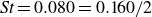
We consider the two-dimensional incompressible flow across two side-by-side square cylinders (prisms) separated by a gap distance equal to the prism side $D$
, see figure 1(a). The non-dimensional form of the Navier–Stokes equations reads
$D$
, see figure 1(a). The non-dimensional form of the Navier–Stokes equations reads
 \begin{equation} \begin{aligned} \frac {\partial \boldsymbol{u}}{\partial t} + \boldsymbol{u} \boldsymbol{\cdot }\boldsymbol{\nabla }\boldsymbol{u} & = - \boldsymbol{\nabla }\!p + \frac {1}{\textit{Re}} \Delta \boldsymbol{u}, \\ \boldsymbol{\nabla } \boldsymbol{\cdot }\boldsymbol{u} & = 0, \end{aligned} \end{equation}
where $ \boldsymbol{u} = (u,v)$
is the velocity vector with components
$ \boldsymbol{u} = (u,v)$
is the velocity vector with components $u$
and
$u$
and $v$
in the streamwise (
$v$
in the streamwise ( $x$
) and cross-stream directions (
$x$
) and cross-stream directions ( $y$
), respectively,
$y$
), respectively, $p$
is the pressure, and
$p$
is the pressure, and $\varDelta$
the Laplacian operator. The reference quantities used for non-dimensionalisation are
$\varDelta$
the Laplacian operator. The reference quantities used for non-dimensionalisation are $D$
for the spatial variables, the free stream velocity
$D$
for the spatial variables, the free stream velocity $U_{\infty }$
for velocities and
$U_{\infty }$
for velocities and $ \rho U_{\infty }^2$
for pressure (where
$ \rho U_{\infty }^2$
for pressure (where $ \rho$
is the fluid density). In the following, an overbar denotes a time-average quantity and a prime the fluctuation; for example,
$ \rho$
is the fluid density). In the following, an overbar denotes a time-average quantity and a prime the fluctuation; for example, $u=\overline {u}+u^\prime$
denotes the Reynolds decomposition of the instantaneous streamwise velocity
$u=\overline {u}+u^\prime$
denotes the Reynolds decomposition of the instantaneous streamwise velocity $u$
. The origin of the coordinate system
$u$
. The origin of the coordinate system $(x,y)$
is located at the centreline, in the gap between the cylinders, midway across the side length
$(x,y)$
is located at the centreline, in the gap between the cylinders, midway across the side length $D$
.
$D$
.
(a) Flow configuration and boundary conditions, (b) global and zoomed-in views of mesh 2.

The Reynolds number is defined as $\textit{Re} = U_{\infty } D / \nu$
, where
$\textit{Re} = U_{\infty } D / \nu$
, where $ \nu$
is the kinematic viscosity of the fluid. We simulate the flow at
$ \nu$
is the kinematic viscosity of the fluid. We simulate the flow at $\textit{Re}=200$
. At this value, the vortex shedding from the top and bottom cylinders is temporally irregular (Ma et al. Reference Ma, Kang, Lim, Wu and Tutty2017). The non-dimensional frequency is defined as
$\textit{Re}=200$
. At this value, the vortex shedding from the top and bottom cylinders is temporally irregular (Ma et al. Reference Ma, Kang, Lim, Wu and Tutty2017). The non-dimensional frequency is defined as $\textit{St}=\textit{fD}/U_{\infty }$
.
$\textit{St}=\textit{fD}/U_{\infty }$
.
The equations are discretised using the finite-volume methodology applied to a Cartesian mesh. Uniform velocity is imposed at the inlet, zero pressure gradient at the outlet, and symmetry conditions at the top and bottom boundaries. The Crank–Nicolson scheme is employed for time marching with time step $\delta t=0.01$
. The convective and viscous terms are discretised using a second-order central scheme. The flow was simulated for
$\delta t=0.01$
. The convective and viscous terms are discretised using a second-order central scheme. The flow was simulated for $500$
time units (one time unit is equal to
$500$
time units (one time unit is equal to $D/U_{\infty }$
) until a fully developed flow was obtained. The simulation was then restarted and continued over
$D/U_{\infty }$
) until a fully developed flow was obtained. The simulation was then restarted and continued over $ 10\,000$
time units, during which data were collected for further processing.
$ 10\,000$
time units, during which data were collected for further processing.
To assess the accuracy of the simulation, a mesh independence study was conducted. Simulations were carried out with three meshes, 1, 2 and 3, consisting of 66 258, 84 253 and 99 478 cells respectively. Mesh 2 is shown in figure 1(b). Table 1 summarises relevant mesh details and the computed mean and root mean square (r.m.s.) values of the lift ( $C_{\!L}$
) and drag (
$C_{\!L}$
) and drag ( $C_{\!D}$
) coefficients for the bottom cylinder. Comparison with the reference values of Ma et al. (Reference Ma, Kang, Lim, Wu and Tutty2017) confirms the accuracy of the results, especially for Meshes 2 and 3.
$C_{\!D}$
) coefficients for the bottom cylinder. Comparison with the reference values of Ma et al. (Reference Ma, Kang, Lim, Wu and Tutty2017) confirms the accuracy of the results, especially for Meshes 2 and 3.
Mesh details and force coefficients for the bottom cylinder.

Figure 2(a) shows comparison of the $\bar {u}(y)$
velocity profile across the gap at
$\bar {u}(y)$
velocity profile across the gap at $x = 0$
with that of Ma et al. (Reference Ma, Kang, Lim, Wu and Tutty2017). Panel (b) shows the frequency spectrum of the lift coefficient (
$x = 0$
with that of Ma et al. (Reference Ma, Kang, Lim, Wu and Tutty2017). Panel (b) shows the frequency spectrum of the lift coefficient ( $C_{\!L}$
) for the bottom cylinder. There is a clear peak at frequency
$C_{\!L}$
) for the bottom cylinder. There is a clear peak at frequency $\textit{St}=0.168$
; this is further analysed later. The velocity profiles and the spectra exhibit minimal differences between the three meshes, suggesting that the solutions are indeed grid independent. In the following, the flow fields from Mesh 2 are used.
$\textit{St}=0.168$
; this is further analysed later. The velocity profiles and the spectra exhibit minimal differences between the three meshes, suggesting that the solutions are indeed grid independent. In the following, the flow fields from Mesh 2 are used.
Mesh independence study: (a) $\bar {u}(y)$
across the gap between the cylinders at
$\bar {u}(y)$
across the gap between the cylinders at $x=0$
; (b) spectrum of
$x=0$
; (b) spectrum of $C_{\!L}'$
for the bottom cylinder.
$C_{\!L}'$
for the bottom cylinder.

3. Flow characteristics
Figure 3 depicts instantaneous vorticity snapshots at six time instants $t_1 {-} t_6$
. A jet emanates from the gap between the cylinders and disrupts the periodic vortex shedding behind each cylinder, leading to irregular flow patterns (the flow is in fact chaotic, as will be demonstrated in § 4). The jet exhibits a flapping motion which is determined by the pressure field induced by the vortices shed from the prisms’ faces on either side of the gap. In the vorticity snapshots of the top row, the jet bends mainly upwards, while in the bottom row, it bends downwards. Note how the vortices are stretched by the flow, from highly concentrated blobs to long vorticity filaments. Notice also the long excursions of the wake in the cross-stream direction. Vortex filaments can reach
$t_1 {-} t_6$
. A jet emanates from the gap between the cylinders and disrupts the periodic vortex shedding behind each cylinder, leading to irregular flow patterns (the flow is in fact chaotic, as will be demonstrated in § 4). The jet exhibits a flapping motion which is determined by the pressure field induced by the vortices shed from the prisms’ faces on either side of the gap. In the vorticity snapshots of the top row, the jet bends mainly upwards, while in the bottom row, it bends downwards. Note how the vortices are stretched by the flow, from highly concentrated blobs to long vorticity filaments. Notice also the long excursions of the wake in the cross-stream direction. Vortex filaments can reach $y$
values larger than
$y$
values larger than $4$
; this is due to the sweeping motion of the flapping jet.
$4$
; this is due to the sweeping motion of the flapping jet.
Contour plots of instantaneous vorticity ( $\boldsymbol{\nabla }\times \boldsymbol{u}$
) at six time instances. The plots depict the flapping motion of the jet and the merging of vortices 1 and 2. For an animation of vorticity contours, see supplementary movie 1 available at https://doi.org/10.1017/jfm.2026.11489.
$\boldsymbol{\nabla }\times \boldsymbol{u}$
) at six time instances. The plots depict the flapping motion of the jet and the merging of vortices 1 and 2. For an animation of vorticity contours, see supplementary movie 1 available at https://doi.org/10.1017/jfm.2026.11489.

Close examination of the vorticity sequences reveals an interesting phenomenon. To visualise it, two clockwise-rotating vortices, marked with numbers 1 and 2, are tracked. The vortices are shed from the top face of each prism. At time instant $t_1$
, the two vortices are highly concentrated and almost in phase. At the subsequent time instants
$t_1$
, the two vortices are highly concentrated and almost in phase. At the subsequent time instants $t_2$
and
$t_2$
and $t_3$
, vortex 1 is stretched and bends downwards coming in close proximity with vortex 2 which, at the same time, moves upwards. At
$t_3$
, vortex 1 is stretched and bends downwards coming in close proximity with vortex 2 which, at the same time, moves upwards. At $t_4$
, the two vortices have moved downstream together and start to merge. The merging process is finished at
$t_4$
, the two vortices have moved downstream together and start to merge. The merging process is finished at $t_5$
and a single vortex is formed that is carried downstream, see instant
$t_5$
and a single vortex is formed that is carried downstream, see instant $t_6$
. This process of vortex merging is an important characteristic of this flow. It can be detected in the spectra and the Lyapunov covariant vectors, as will be seen later.
$t_6$
. This process of vortex merging is an important characteristic of this flow. It can be detected in the spectra and the Lyapunov covariant vectors, as will be seen later.
Frequency spectrum of the fluctuating force coefficients for (a) $C_{\!L}^\prime$
and (b)
$C_{\!L}^\prime$
and (b) $C_{\!D}^\prime$
of the two prisms.
$C_{\!D}^\prime$
of the two prisms.

The flow irregularity leaves its footprint on the spectra of the fluctuating $C_{\!L}^\prime$
and
$C_{\!L}^\prime$
and $C_{\!D}^\prime$
coefficients shown in figure 4. The spectra were computed with Welch’s method using eight segments with 20 % overlap and a Hamming window on each segment. They are almost identical for the top and bottom prisms, as expected due to symmetry. This also indicates that the signal is long enough that can capture the matching of the spectra at low frequencies. In the
$C_{\!D}^\prime$
coefficients shown in figure 4. The spectra were computed with Welch’s method using eight segments with 20 % overlap and a Hamming window on each segment. They are almost identical for the top and bottom prisms, as expected due to symmetry. This also indicates that the signal is long enough that can capture the matching of the spectra at low frequencies. In the $C_{\!D}$
spectrum, there are two peaks at
$C_{\!D}$
spectrum, there are two peaks at $\textit{St}_{1}=0.063$
and
$\textit{St}_{1}=0.063$
and $\textit{St}_{2}=0.168$
(the former stronger than the latter), whereas the
$\textit{St}_{2}=0.168$
(the former stronger than the latter), whereas the $C_{\!L}$
spectrum exhibits only one peak at
$C_{\!L}$
spectrum exhibits only one peak at $\textit{St}_{2}=0.168$
. Note however that multiple smaller peaks appear, especially around
$\textit{St}_{2}=0.168$
. Note however that multiple smaller peaks appear, especially around $\textit{St}_2$
, due to the flow irregularity. Two main frequency bands can be identified, a lower band (
$\textit{St}_2$
, due to the flow irregularity. Two main frequency bands can be identified, a lower band ( $\textit{St}\in [0.057,0.068]$
) around
$\textit{St}\in [0.057,0.068]$
) around $\textit{St}_{1}$
and an upper band (
$\textit{St}_{1}$
and an upper band ( $\textit{St}\in [0.155,0.174]$
) around
$\textit{St}\in [0.155,0.174]$
) around $\textit{St}_{2}$
. Notice also the presence of a weaker peak at the subharmonic
$\textit{St}_{2}$
. Notice also the presence of a weaker peak at the subharmonic $\textit{St}_2/2=0.084$
in the
$\textit{St}_2/2=0.084$
in the $C_{\!D}$
spectrum; a third band
$C_{\!D}$
spectrum; a third band $\bigl (St\in [0.073,0.089]\bigr )$
is marked around it. The bandwidths are determined by the full width at half maximum (FWHM) of the corresponding spectral peak, see Bhattacharya & Gregory (Reference Bhattacharya and Gregory2015).
$\bigl (St\in [0.073,0.089]\bigr )$
is marked around it. The bandwidths are determined by the full width at half maximum (FWHM) of the corresponding spectral peak, see Bhattacharya & Gregory (Reference Bhattacharya and Gregory2015).
Spectra of the transverse velocity $v(x,y)$
at (a)
$v(x,y)$
at (a) $x=2$
, (b)
$x=2$
, (b) $10$
and (c)
$10$
and (c) $20$
. Top row shows along the gap centreline (
$20$
. Top row shows along the gap centreline ( $y=0$
); bottom row shows along the centreline behind the top prism (
$y=0$
); bottom row shows along the centreline behind the top prism ( $y=1$
). The shaded regions mark the frequency bands defined in figure 4.
$y=1$
). The shaded regions mark the frequency bands defined in figure 4.

To explain the physical mechanisms behind $\textit{St}_1$
and
$\textit{St}_1$
and $\textit{St}_2$
, we compute the spectra of the transverse velocity
$\textit{St}_2$
, we compute the spectra of the transverse velocity $v(x,y)$
at three locations
$v(x,y)$
at three locations $x=2$
,
$x=2$
, $10$
and
$10$
and $20$
along
$20$
along $y=0$
(gap centreline) and
$y=0$
(gap centreline) and $y=1$
(centreline behind top square cylinder). The results are shown in figure 5. At point
$y=1$
(centreline behind top square cylinder). The results are shown in figure 5. At point $x=2,\ y=0$
, the flow physics is determined by the jet motion and the power spectral density (PSD) exhibits a pronounced peak at
$x=2,\ y=0$
, the flow physics is determined by the jet motion and the power spectral density (PSD) exhibits a pronounced peak at $0.061$
which is very close to
$0.061$
which is very close to $\textit{St}_1$
, indicating that the latter corresponds to the low-frequency flapping motion. It is interesting to note that the prominent peak in the
$\textit{St}_1$
, indicating that the latter corresponds to the low-frequency flapping motion. It is interesting to note that the prominent peak in the $C_{\!D}$
spectrum is therefore caused by the gap-jet flapping. At the same streamwise location but at
$C_{\!D}$
spectrum is therefore caused by the gap-jet flapping. At the same streamwise location but at $y=1$
, the PSD peaks at
$y=1$
, the PSD peaks at $0.171$
, which is close to
$0.171$
, which is close to $\textit{St}_2$
, indicating that the latter represents the primary vortex shedding frequency in the wake behind the individual prisms. Thus, vortex shedding explains the main peak in
$\textit{St}_2$
, indicating that the latter represents the primary vortex shedding frequency in the wake behind the individual prisms. Thus, vortex shedding explains the main peak in $C_{\!L}$
spectrum and the secondary peak in the
$C_{\!L}$
spectrum and the secondary peak in the $C_{\!D}$
spectrum. It is very interesting to note that further downstream (
$C_{\!D}$
spectrum. It is very interesting to note that further downstream ( $x=10$
and
$x=10$
and $20$
) at both
$20$
) at both $y$
lines, the PSD peaks converge to a single peak at
$y$
lines, the PSD peaks converge to a single peak at $0.073$
, which is within the subharmonic frequency band.
$0.073$
, which is within the subharmonic frequency band.
Streamwise evolution of the dominant $\textit{St}$
of the
$\textit{St}$
of the $v$
velocity spectrum along (a)
$v$
velocity spectrum along (a) $y=0$
and (b)
$y=0$
and (b) $y=1$
. The shaded regions mark the frequency bands defined in figure 4.
$y=1$
. The shaded regions mark the frequency bands defined in figure 4.

Figure 6 shows the dominant $\textit{St}$
of the PSD of
$\textit{St}$
of the PSD of $v(x,y)$
along
$v(x,y)$
along $x$
for both
$x$
for both $y$
lines. In the near wake (
$y$
lines. In the near wake ( $x\lesssim 4$
), the dominant frequency is within the upper frequency band (i.e. close to
$x\lesssim 4$
), the dominant frequency is within the upper frequency band (i.e. close to $\textit{St}_{2}$
) at
$\textit{St}_{2}$
) at $y=1$
and within the lower band (i.e. close to
$y=1$
and within the lower band (i.e. close to $\textit{St}_{1}$
) at
$\textit{St}_{1}$
) at $y=0$
, confirming the different mechanisms behind each band. However, downstream of
$y=0$
, confirming the different mechanisms behind each band. However, downstream of $x \approx 5$
, the dominant
$x \approx 5$
, the dominant $\textit{St}$
drops to approximately
$\textit{St}$
drops to approximately $\textit{St}_{2}/2$
, consistent with the subharmonic generated by vortex pairing events such as the one shown in figure 3. The spatial location of the frequency drop matches very closely with the merging location depicted in the aforementioned figure. This frequency shift marks the onset of wake dynamics dominated by paired vortices and the decay of the gap-jet oscillation. The association of vortex merging with the subharmonic has been reported repeatedly in the literature, see Meiburg (Reference Meiburg1987), Shaabani-Ardali, Sipp & Lesshafft (Reference Shaabani-Ardali, Sipp and Lesshafft2019).
$\textit{St}_{2}/2$
, consistent with the subharmonic generated by vortex pairing events such as the one shown in figure 3. The spatial location of the frequency drop matches very closely with the merging location depicted in the aforementioned figure. This frequency shift marks the onset of wake dynamics dominated by paired vortices and the decay of the gap-jet oscillation. The association of vortex merging with the subharmonic has been reported repeatedly in the literature, see Meiburg (Reference Meiburg1987), Shaabani-Ardali, Sipp & Lesshafft (Reference Shaabani-Ardali, Sipp and Lesshafft2019).
Contours of the time-averaged streamwise velocity $\bar {u}$
superimposed to streamlines.
$\bar {u}$
superimposed to streamlines.

Despite the underlying irregular dynamics, the time-averaged streamwise velocity field $\bar {u}$
, shown in figure 7, is symmetric about
$\bar {u}$
, shown in figure 7, is symmetric about $y=0$
. A high-speed jet emerges from the gap and two symmetric recirculation zones form immediately downstream of the cylinders. The coexistence of the jet and the recirculation zones results in a highly non-uniform velocity field in the very near wake. Further downstream the flow behind the cylinders recovers and the jet velocity decays, making the velocity profiles in the cross-stream direction more uniform.
$y=0$
. A high-speed jet emerges from the gap and two symmetric recirculation zones form immediately downstream of the cylinders. The coexistence of the jet and the recirculation zones results in a highly non-uniform velocity field in the very near wake. Further downstream the flow behind the cylinders recovers and the jet velocity decays, making the velocity profiles in the cross-stream direction more uniform.
3.1. Spectral proper orthogonal decomposition (SPOD) of the flow
To obtain more insight, SPOD (Towne, Schmidt & Colonius Reference Towne, Schmidt and Colonius2018) is applied to the fluctuating flow field. The method will identify the structures beating at the dominant frequencies identified earlier. A total of $K = 100\,000$
snapshots of velocity perturbations obtained every
$K = 100\,000$
snapshots of velocity perturbations obtained every $\delta t=0.01$
are stacked column by column to form matrix
$\delta t=0.01$
are stacked column by column to form matrix $Y$
,
$Y$
,
 \begin{equation} Y = \left [\begin{array}{cccc} {u^{\prime }_1}^{(1)} & {u^{\prime }_1}^{(2)} & {\cdots} & {u^{\prime }_1}^{(K)} \\[3pt] {v^{\prime }_1}^{(1)} & {v^{\prime }_1}^{(2)} & {\cdots} & {v^{\prime }_1}^{(K)} \\[3pt] \vdots & \vdots & {\cdots} & \vdots \\[3pt] {u^{\prime }_N}^{(1)} & {u^{\prime }_N}^{(2)} & {\cdots} & {u^{\prime }_N}^{(K)} \\[3pt] {v^{\prime }_N}^{(1)} & {v^{\prime }_N}^{(2)} & {\cdots} & {v^{\prime }_N}^{(K)} \end{array}\right ]\!. \end{equation}
The superscripts denote the snapshot index $k = 1, 2, \ldots , K$
and the subscripts the cell number
$k = 1, 2, \ldots , K$
and the subscripts the cell number $n = 1, 2, \ldots , N$
, where
$n = 1, 2, \ldots , N$
, where $N=84\,253$
(cell count of mesh 2). Matrix
$N=84\,253$
(cell count of mesh 2). Matrix $Y$
is divided into 11 blocks with a 50 % overlap. For each frequency
$Y$
is divided into 11 blocks with a 50 % overlap. For each frequency $\textit{St}_k$
, a cross-spectral density (CSD) matrix
$\textit{St}_k$
, a cross-spectral density (CSD) matrix $ \boldsymbol{S}(St_k)$
is formed and the SPOD eigenvalue problem is solved to find the SPOD modes
$ \boldsymbol{S}(St_k)$
is formed and the SPOD eigenvalue problem is solved to find the SPOD modes $ \varPhi ^{st_k}$
and their energies
$ \varPhi ^{st_k}$
and their energies $ \lambda (St_k)$
. Since the CSD matrix is Hermitian, the eigenvalues are real but the eigenvectors (SPOD modes) are complex, i.e.
$ \lambda (St_k)$
. Since the CSD matrix is Hermitian, the eigenvalues are real but the eigenvectors (SPOD modes) are complex, i.e. $ \varPhi ^{St_k} = \varPhi _r^{St_k} + i \varPhi _i^{St_k}$
; for more details, see Towne et al. (Reference Towne, Schmidt and Colonius2018).
$ \varPhi ^{St_k} = \varPhi _r^{St_k} + i \varPhi _i^{St_k}$
; for more details, see Towne et al. (Reference Towne, Schmidt and Colonius2018).
Variation of SPOD mode energies (eigenvalues) across frequency.

Figure 8 presents the variation of SPOD eigenvalues across frequency. Mode 1 refers to the leading SPOD mode at each frequency. Each curve represents the energy of the corresponding SPOD mode at different frequencies. Mode 1 exhibits two clear peaks at $0.063$
and
$0.063$
and $0.160$
that match closely
$0.160$
that match closely $\textit{St}_1$
and
$\textit{St}_1$
and $\textit{St}_2$
, respectively, of the
$\textit{St}_2$
, respectively, of the $C_{\!D}$
spectrum. For the lower frequency band, the energy of mode 1 is markedly higher than that of mode 2, indicating that the gap-jet flapping motion is well approximated by just one mode. In the higher frequency band, the energy separation between modes 1 and 2 is not so pronounced. Note also the presence of a band with
$C_{\!D}$
spectrum. For the lower frequency band, the energy of mode 1 is markedly higher than that of mode 2, indicating that the gap-jet flapping motion is well approximated by just one mode. In the higher frequency band, the energy separation between modes 1 and 2 is not so pronounced. Note also the presence of a band with $0.080$
, the subharmonic of the
$0.080$
, the subharmonic of the $0.160$
.
$0.160$
.
Contour plots of streamwise (left column) and cross-stream (right column) velocities of the real part of SPOD mode 1 at (a) $ St = 0.063$
,
$ St = 0.063$
, $\varPhi _{1r}^{0.063}$
, (b)
$\varPhi _{1r}^{0.063}$
, (b) $\textit{St}=0.160$
,
$\textit{St}=0.160$
, $\varPhi _{1r}^{0.160}$
and (c)
$\varPhi _{1r}^{0.160}$
and (c) $ St = 0.080$
,
$ St = 0.080$
, $\varPhi _{1r}^{0.080}$
.
$\varPhi _{1r}^{0.080}$
.

Figure 9 shows contours of the streamwise ( $u$
) and transverse (
$u$
) and transverse ( $v$
) velocities of the real part of SPOD mode 1 at
$v$
) velocities of the real part of SPOD mode 1 at $\textit{St}=0.063$
,
$\textit{St}=0.063$
, $0.160$
and the subharmonic
$0.160$
and the subharmonic $0.080$
. At
$0.080$
. At $\textit{St} = 0.063$
, the
$\textit{St} = 0.063$
, the $v$
contours peak at the gap centreline in the near wake. Both
$v$
contours peak at the gap centreline in the near wake. Both $u$
and
$u$
and $v$
reach their maxima at
$v$
reach their maxima at $x \approx 4$
, precisely where the jet-flapping motion is most discernible. At
$x \approx 4$
, precisely where the jet-flapping motion is most discernible. At $\textit{St} = 0.160$
(the vortex-shedding frequency), a train of small-scale structures appears in the wake of each prism in the
$\textit{St} = 0.160$
(the vortex-shedding frequency), a train of small-scale structures appears in the wake of each prism in the $v$
contours. The peaks now appear behind the prisms, not in the gap centreline. Notice that the peaks are displaced further away from the centreline as
$v$
contours. The peaks now appear behind the prisms, not in the gap centreline. Notice that the peaks are displaced further away from the centreline as $x$
increases, indicating the wake expansion. The
$x$
increases, indicating the wake expansion. The $v$
field is antisymmetric with respect to the gap centreline, but the
$v$
field is antisymmetric with respect to the gap centreline, but the $u$
field is symmetric. The
$u$
field is symmetric. The $v$
mode attains maximum values in the near-wake region (
$v$
mode attains maximum values in the near-wake region ( $x\lt 4$
), as for
$x\lt 4$
), as for $\textit{St}=0.063$
. However, the
$\textit{St}=0.063$
. However, the $v$
contours of the subharmonic at
$v$
contours of the subharmonic at $\textit{St}=0.080=0.160/2$
) grow rapidly in the near wake (where vortex merging occurs), peaks in the mid-wake
$\textit{St}=0.080=0.160/2$
) grow rapidly in the near wake (where vortex merging occurs), peaks in the mid-wake $x \in [12,20]$
and then decays.
$x \in [12,20]$
and then decays.
Overall, the dominant SPOD mode captures the three key phenomena identified earlier: jet-flapping, vortex shedding behind each cylinder and vortex pairing. As can be seen in the SPOD energy spectrum, gap-jet-flapping carries the largest energy, followed by vortex pairing and then asynchronous shedding.
Having characterised the main features of the flow, the next step is to consider the flow as a dynamical system, and analyse the Lyapunov exponents (LEs) and covariant Lyapunov vectors (CLVs). A key objective is to explore the footprint of the above-mentioned features onto the CLVs.
4. Analysis of the flow from a dynamical systems perspective
4.1. Lyapunov exponents
After discretisation, the system of governing equations (2.1) can be put in the general form,
 \begin{equation} \frac {{\rm d} \boldsymbol{u}}{{\rm d}t} = \boldsymbol{f}\!\left (\boldsymbol{u}\right ), \quad \boldsymbol{u}(0) = \boldsymbol{u}_0, \end{equation}
where $\boldsymbol{u}(t)$
is the state vector
$\boldsymbol{u}(t)$
is the state vector $\boldsymbol{u}(t) = \{u_1(t), v_1(t), \ldots , u_{N}(t), v_{N}(t)\} \in \mathbb{R}^{2N}$
, and
$\boldsymbol{u}(t) = \{u_1(t), v_1(t), \ldots , u_{N}(t), v_{N}(t)\} \in \mathbb{R}^{2N}$
, and $N$
is the number of cells. To get (4.1), we have used the continuity equation to eliminate pressure. This is done by constructing a Poisson equation for pressure (Pope Reference Pope2000), which can be notionally solved, and thus,
$N$
is the number of cells. To get (4.1), we have used the continuity equation to eliminate pressure. This is done by constructing a Poisson equation for pressure (Pope Reference Pope2000), which can be notionally solved, and thus, $\boldsymbol{\nabla }\!P$
can be expressed in terms of velocities. As the dynamical system evolves, the state vector traces a trajectory in phase space. We define the evolution operator
$\boldsymbol{\nabla }\!P$
can be expressed in terms of velocities. As the dynamical system evolves, the state vector traces a trajectory in phase space. We define the evolution operator $\mathcal{L}^{t}$
that maps
$\mathcal{L}^{t}$
that maps $\boldsymbol{u}(0)$
to
$\boldsymbol{u}(0)$
to $\boldsymbol{u}(t)$
under the dynamics (4.1),
$\boldsymbol{u}(t)$
under the dynamics (4.1), $\mathcal{L}^{t}(\boldsymbol{u}(0)) =\boldsymbol{u}(t)$
.
$\mathcal{L}^{t}(\boldsymbol{u}(0)) =\boldsymbol{u}(t)$
.
A key concept in dynamical systems is ergodicity, which implies that the time-average state of the system is independent of the initial condition (Birkhoff Reference Birkhoff1931). For ergodic systems, the long-time trajectory converges to a bounded region in phase space known as attractor (Ruelle Reference Ruelle1980). Attractors can be classified into three types: fixed (or equilibrium) points, limit cycles and strange attractors. Fixed-point attractors are stable points that trajectories converge to over time, limit-cycle attractors correspond to stable periodic orbits and strange attractors represent chaotic systems that exhibit complex, irregular patterns (as the one considered in this study).
We define our (assumed ergodic) dynamical system in the $2N$
-dimensional Riemannian manifold
$2N$
-dimensional Riemannian manifold $\mathcal{M}$
. The Oseledets (Reference Oseledets1968) theorem establishes that a set of Lyapunov exponents (LEs) exists, provided there is a tangent space
$\mathcal{M}$
. The Oseledets (Reference Oseledets1968) theorem establishes that a set of Lyapunov exponents (LEs) exists, provided there is a tangent space $\mathcal{T}_{\boldsymbol{u}} \mathcal{M}$
that describes the local geometry of the attractor for every state
$\mathcal{T}_{\boldsymbol{u}} \mathcal{M}$
that describes the local geometry of the attractor for every state $\boldsymbol{u}(t)$
. Here,
$\boldsymbol{u}(t)$
. Here, $\mathcal{T}_{\boldsymbol{u}} \mathcal{M}$
is a
$\mathcal{T}_{\boldsymbol{u}} \mathcal{M}$
is a $2N$
-dimensional vector space consisting of all the possible directions in which the state
$2N$
-dimensional vector space consisting of all the possible directions in which the state $\boldsymbol{u}(t)$
can be perturbed. To study the response of a dynamical system to an arbitrary perturbation
$\boldsymbol{u}(t)$
can be perturbed. To study the response of a dynamical system to an arbitrary perturbation $\boldsymbol{\delta \boldsymbol{u}} \in \mathcal{T}_{\boldsymbol{u}} \mathcal{M}$
, we define the local expansion rate as
$\boldsymbol{\delta \boldsymbol{u}} \in \mathcal{T}_{\boldsymbol{u}} \mathcal{M}$
, we define the local expansion rate as
 \begin{equation} \gamma \!\left ( \boldsymbol{\delta \boldsymbol{u}}, \boldsymbol{u},t \right ) = \frac {\left \|D \mathcal{L}^t(\boldsymbol{u}) \boldsymbol{\delta \boldsymbol{u}} \right \|}{\| \boldsymbol{\delta \boldsymbol{u}}\|} ,\end{equation}
where $\|\boldsymbol{\cdot }\|$
denotes the Euclidean norm and
$\|\boldsymbol{\cdot }\|$
denotes the Euclidean norm and $D \mathcal{L}^t(\boldsymbol{u})$
is the linear evolution operator of the tangent space. More specifically,
$D \mathcal{L}^t(\boldsymbol{u})$
is the linear evolution operator of the tangent space. More specifically, $D \mathcal{L}^t(\boldsymbol{u})$
evolves the linearised form of (4.1) around
$D \mathcal{L}^t(\boldsymbol{u})$
evolves the linearised form of (4.1) around $\boldsymbol{u}$
,
$\boldsymbol{u}$
,
 \begin{equation} \frac {\partial (\boldsymbol{\delta \boldsymbol{u}})}{\partial t}= \frac {\partial \! \boldsymbol{f} }{\partial \boldsymbol{u} } \delta \boldsymbol{u}, \end{equation}
over a time window $t$
. In other words, if the perturbation at the start of the time window is
$t$
. In other words, if the perturbation at the start of the time window is $\boldsymbol{\delta \boldsymbol{u}}$
, the notation
$\boldsymbol{\delta \boldsymbol{u}}$
, the notation $D \mathcal{L}^t(\boldsymbol{u}) \boldsymbol{\delta \boldsymbol{u}}$
is the result of the action of this operator, i.e.
$D \mathcal{L}^t(\boldsymbol{u}) \boldsymbol{\delta \boldsymbol{u}}$
is the result of the action of this operator, i.e. $D \mathcal{L}^t(\boldsymbol{u}) \boldsymbol{\delta \boldsymbol{u}}=\boldsymbol{\delta \boldsymbol{u}}(t)$
. Thus, the operator performs the mapping
$D \mathcal{L}^t(\boldsymbol{u}) \boldsymbol{\delta \boldsymbol{u}}=\boldsymbol{\delta \boldsymbol{u}}(t)$
. Thus, the operator performs the mapping $\mathcal{T}_{\boldsymbol{u}} \mathcal{M} \rightarrow \mathcal{T}_{\mathcal{L}^t(\boldsymbol{u})} \mathcal{M}$
. For the Navier–Stokes equations, the linearised form is
$\mathcal{T}_{\boldsymbol{u}} \mathcal{M} \rightarrow \mathcal{T}_{\mathcal{L}^t(\boldsymbol{u})} \mathcal{M}$
. For the Navier–Stokes equations, the linearised form is
 \begin{equation} \begin{aligned} \frac {\partial (\boldsymbol{\delta \boldsymbol{u}})}{\partial t}+ \boldsymbol{u} \boldsymbol{\cdot }\boldsymbol{\nabla }(\boldsymbol{\delta \boldsymbol{u}}) +\boldsymbol{\delta \boldsymbol{u}} \boldsymbol{\cdot }\boldsymbol{\nabla }\boldsymbol{u} & =-\boldsymbol{\nabla }(\delta p)+\frac {1}{\textit{Re}} \Delta (\boldsymbol{\delta \boldsymbol{u}}), \\ \boldsymbol{\nabla }\boldsymbol{\cdot }(\boldsymbol{\delta \boldsymbol{u}}) & =0, \end{aligned} \end{equation}
where $\boldsymbol{\delta \boldsymbol{u}}= (\delta u, \delta v)$
.
$\boldsymbol{\delta \boldsymbol{u}}= (\delta u, \delta v)$
.
The Lyapunov exponent $\lambda$
associated with the perturbation vector
$\lambda$
associated with the perturbation vector $\boldsymbol{\delta \boldsymbol{u}}$
is the long-time average,
$\boldsymbol{\delta \boldsymbol{u}}$
is the long-time average,
 \begin{equation} \lambda (\boldsymbol{\delta \boldsymbol{u}}) = \lim _{t \rightarrow \infty } \frac {1}{t} \ln \frac {\left \|D \mathcal{L}^t(\boldsymbol{u}) \boldsymbol{\delta \boldsymbol{u}}\right \|}{\| \boldsymbol{\delta \boldsymbol{u}}\|} .\end{equation}
This exponent represents the average exponential rate of expansion (or contraction) of the perturbation $\boldsymbol{\delta \boldsymbol{u}}$
, i.e.
$\boldsymbol{\delta \boldsymbol{u}}$
, i.e. $\left \| \boldsymbol{\delta \boldsymbol{u}}(t)\right \| \sim \| \boldsymbol{\delta \boldsymbol{u}}(0)\| \mathrm{e}^{\lambda t}$
. The Oseledets (Reference Oseledets1968) theorem establishes that
$\left \| \boldsymbol{\delta \boldsymbol{u}}(t)\right \| \sim \| \boldsymbol{\delta \boldsymbol{u}}(0)\| \mathrm{e}^{\lambda t}$
. The Oseledets (Reference Oseledets1968) theorem establishes that $\lambda$
assumes a finite number of distinct values
$\lambda$
assumes a finite number of distinct values $\lambda _1 \gt \lambda _2 \gt {\cdots} \gt \lambda _m$
, where
$\lambda _1 \gt \lambda _2 \gt {\cdots} \gt \lambda _m$
, where $m \leqslant 2N$
, as the perturbation vector
$m \leqslant 2N$
, as the perturbation vector $\boldsymbol{\delta \boldsymbol{u}}$
varies in the tangent space
$\boldsymbol{\delta \boldsymbol{u}}$
varies in the tangent space $\mathcal{T}_{\boldsymbol{u}} \mathcal{M}$
.
$\mathcal{T}_{\boldsymbol{u}} \mathcal{M}$
.
The set of LEs, known as the ‘Lyapunov spectrum’, is a characteristic of the dynamical system. In a chaotic dynamical system, there is at least one positive LE, i.e. $\lambda _1 \gt 0$
. This means that the perturbed trajectory
$\lambda _1 \gt 0$
. This means that the perturbed trajectory $ \boldsymbol{\boldsymbol{u}}(t)+\boldsymbol{\delta \boldsymbol{u}}(t)$
will diverge exponentially from the reference trajectory
$ \boldsymbol{\boldsymbol{u}}(t)+\boldsymbol{\delta \boldsymbol{u}}(t)$
will diverge exponentially from the reference trajectory $ \boldsymbol{\boldsymbol{u}}(t)$
at an average rate
$ \boldsymbol{\boldsymbol{u}}(t)$
at an average rate $\lambda _1$
.
$\lambda _1$
.
When a randomly chosen set of $m \leqslant 2N$
infinitesimal perturbations
$m \leqslant 2N$
infinitesimal perturbations $(\boldsymbol{\delta \boldsymbol{u}}_1, \boldsymbol{\delta \boldsymbol{u}}_2,{} \ldots , \boldsymbol{\delta \boldsymbol{u}}_m)$
are propagated in the tangent space using (4.3) (or (4.4) in our case), the angles between
$(\boldsymbol{\delta \boldsymbol{u}}_1, \boldsymbol{\delta \boldsymbol{u}}_2,{} \ldots , \boldsymbol{\delta \boldsymbol{u}}_m)$
are propagated in the tangent space using (4.3) (or (4.4) in our case), the angles between $\boldsymbol{\delta \boldsymbol{u}}_i$
reduce with time as all perturbations align along the most unstable direction. Thus, one can compute only the leading LE: identifying smaller LEs becomes numerically ill-conditioned. Benettin et al. (Reference Benettin, Galgani, Giorgilli and Strelcyn1980a
,Reference Benettin, Galgani, Giorgilli and Strelcyn
b
) devised an algorithm in which the set of
$\boldsymbol{\delta \boldsymbol{u}}_i$
reduce with time as all perturbations align along the most unstable direction. Thus, one can compute only the leading LE: identifying smaller LEs becomes numerically ill-conditioned. Benettin et al. (Reference Benettin, Galgani, Giorgilli and Strelcyn1980a
,Reference Benettin, Galgani, Giorgilli and Strelcyn
b
) devised an algorithm in which the set of $m$
perturbations is propagated for a time interval
$m$
perturbations is propagated for a time interval $t_{\textit{step}}$
; the evolved
$t_{\textit{step}}$
; the evolved ${\boldsymbol{\delta \boldsymbol{u}}}_i$
are then orthonormalised and replaced by a set of orthonormal vectors that span the same subspace. These vectors are used as initial conditions and are propagated for another time segment
${\boldsymbol{\delta \boldsymbol{u}}}_i$
are then orthonormalised and replaced by a set of orthonormal vectors that span the same subspace. These vectors are used as initial conditions and are propagated for another time segment $t_{\textit{step}}$
. Benettin et al. (Reference Benettin, Galgani, Giorgilli and Strelcyn1980a
) proved that using Gram–Schmidt QR decomposition, a set of coordinate-independent LEs can be obtained. Coordinate independence means that the computed LEs are intrinsic to the system dynamics and therefore independent of the chosen coordinate system, and thus the norm used to compute them, see also Bewley (Reference Bewley1999). The process is presented in algorithm 1.
$t_{\textit{step}}$
. Benettin et al. (Reference Benettin, Galgani, Giorgilli and Strelcyn1980a
) proved that using Gram–Schmidt QR decomposition, a set of coordinate-independent LEs can be obtained. Coordinate independence means that the computed LEs are intrinsic to the system dynamics and therefore independent of the chosen coordinate system, and thus the norm used to compute them, see also Bewley (Reference Bewley1999). The process is presented in algorithm 1.
Calculation of Lyapunov exponents (Benettin et al. Reference Benettin, Galgani, Giorgilli and Strelcyn1980a )

Convergence of LEs and forward-backward evolution to calculate CLVs for $t_{\textit{step}} = 0.3$
.
$t_{\textit{step}} = 0.3$
.

To compute the LEs of the flow under consideration, we evolve six orthonormal perturbations $\{\boldsymbol{\delta \boldsymbol{u}} \}_{i=1 \ldots 6}$
in the tangent space. The general perturbations
$\{\boldsymbol{\delta \boldsymbol{u}} \}_{i=1 \ldots 6}$
in the tangent space. The general perturbations $\boldsymbol{\delta \boldsymbol{u}}$
can be expressed as the Fourier integral in the spanwise direction,
$\boldsymbol{\delta \boldsymbol{u}}$
can be expressed as the Fourier integral in the spanwise direction,
 \begin{equation} \boldsymbol{\delta \boldsymbol{u}}(x,y,z,t)=\int _{-\infty }^{+\infty } \boldsymbol{\widehat {\delta {\boldsymbol{u}}}}(x,y,t; \beta ) e^{\iota \beta z}\, {\rm d}\beta ,\end{equation}
and similarly for $\delta p$
. In the present work, we take
$\delta p$
. In the present work, we take $\beta =0$
, i.e. we consider only 2-D perturbations. The perturbations are orthonormalised periodically using Gram–Schmidt QR decomposition. Two segment lengths are chosen
$\beta =0$
, i.e. we consider only 2-D perturbations. The perturbations are orthonormalised periodically using Gram–Schmidt QR decomposition. Two segment lengths are chosen $t_{\textit{step}} = 0.3, 10$
. The convergence of the LEs with the integration time for
$t_{\textit{step}} = 0.3, 10$
. The convergence of the LEs with the integration time for $t_{\textit{step}} = 0.3$
is shown in figure 10. The unstable manifold consists of two positive LEs, which indicates that, on average, perturbations grow exponentially along two directions at any point on the attractor. The leading LE is
$t_{\textit{step}} = 0.3$
is shown in figure 10. The unstable manifold consists of two positive LEs, which indicates that, on average, perturbations grow exponentially along two directions at any point on the attractor. The leading LE is $\lambda _1 \approx 0.1$
. One LE is equal to 0 (neutral manifold) which indicates the absence of growth or decay of perturbations along the trajectory in phase space. Furthermore, the system is non-degenerate as all LEs are distinct (Ginelli et al. Reference Ginelli, Chaté, Livi and Politi2013).
$\lambda _1 \approx 0.1$
. One LE is equal to 0 (neutral manifold) which indicates the absence of growth or decay of perturbations along the trajectory in phase space. Furthermore, the system is non-degenerate as all LEs are distinct (Ginelli et al. Reference Ginelli, Chaté, Livi and Politi2013).
Lyapunov spectrum of the flow.

The LEs were also computed for $t_{\textit{step}} = 10$
, which is approximately one Lyapunov time unit,
$t_{\textit{step}} = 10$
, which is approximately one Lyapunov time unit, $ {1}/{\lambda _1}$
. The LE spectra for the two values of
$ {1}/{\lambda _1}$
. The LE spectra for the two values of $t_{\textit{step}}$
are shown in figure 11. The results are almost identical, confirming the robustness of the calculation.
$t_{\textit{step}}$
are shown in figure 11. The results are almost identical, confirming the robustness of the calculation.
4.2. Covariant Lyapunov vectors
It was shown that LEs converge to constant values when averaged over a long time window. The corresponding directions of growth/decay are known as covariant Lyapunov vectors (CLVs), see Ginelli et al. (Reference Ginelli, Poggi, Turchi, Chaté, Livi and Politi2007, Reference Ginelli, Chaté, Livi and Politi2013). CLVs provide a geometric characterisation of the tangent space. They are unit-norm vectors that span the Gram–Schmidt (GS) subspace and represent the expanding, contracting and neutral directions at each point of the attractor. These directions correspond to the positive, negative and zero LEs, respectively.
The concept of CLVs was first introduced by Oseledets (Reference Oseledets1968) and later formalised as tangent directions of invariant manifolds by Ruelle (Reference Ruelle1979). However, for decades, there were no effective algorithms for their computation. Ginelli et al. (Reference Ginelli, Poggi, Turchi, Chaté, Livi and Politi2007) proposed a stable algorithm to extract CLVs, leveraging the geometric understanding of the tangent space of Ruelle (Reference Ruelle1979). The algorithm is based on a forward-backward evolution of the tangent space. A brief overview is presented in Algorithm 2; the detailed methodology of Ginelli et al. (Reference Ginelli, Chaté, Livi and Politi2013) is presented in Appendix A.
Calculation of covariant Lyapunov vectors (Ginelli et al. Reference Ginelli, Chaté, Livi and Politi2013)

The four phases of the algorithm are shown in figure 10. The algorithm begins with the forward transient phase (in our case, $t \in [0, 2100]$
), in which the dynamical system and six (initially random) orthonormal perturbations are evolved until the tangent subspace and the LE spectrum converge. In the forward dynamics phase (
$t \in [0, 2100]$
), in which the dynamical system and six (initially random) orthonormal perturbations are evolved until the tangent subspace and the LE spectrum converge. In the forward dynamics phase ( $t \in [2100, 4500]$
), the orthonormal Gram–Schmidt vectors
$t \in [2100, 4500]$
), the orthonormal Gram–Schmidt vectors $\boldsymbol{G}_{\!n} = (\boldsymbol{g}_n^{(1)}\mid \boldsymbol{g}_n^{(2)}\mid \ldots \mid \boldsymbol{g}_n^{(6)} )$
and the
$\boldsymbol{G}_{\!n} = (\boldsymbol{g}_n^{(1)}\mid \boldsymbol{g}_n^{(2)}\mid \ldots \mid \boldsymbol{g}_n^{(6)} )$
and the $R_n$
matrices (obtained from the QR decomposition) are stored for every time segment,
$R_n$
matrices (obtained from the QR decomposition) are stored for every time segment, $n$
. In the backward transient phase (
$n$
. In the backward transient phase ( $t \in [5400, 4500]$
), the CLV expansion coefficient matrix
$t \in [5400, 4500]$
), the CLV expansion coefficient matrix $\boldsymbol{C}_{\!n}$
is evolved backwards. To determine the length of this phase,
$\boldsymbol{C}_{\!n}$
is evolved backwards. To determine the length of this phase, $k_2 t_{\textit{step}}$
was increased and the angles between the CLVs in the backward dynamics phase were monitored. At
$k_2 t_{\textit{step}}$
was increased and the angles between the CLVs in the backward dynamics phase were monitored. At $k_2 t_{\textit{step}} = 150$
, the angles between the CLVs stabilised, indicating convergence. In the final backward dynamics phase, the recorded GS matrices
$k_2 t_{\textit{step}} = 150$
, the angles between the CLVs stabilised, indicating convergence. In the final backward dynamics phase, the recorded GS matrices $\boldsymbol{G}_{\!n}$
are multiplied with the expansion coefficient matrices
$\boldsymbol{G}_{\!n}$
are multiplied with the expansion coefficient matrices $\boldsymbol{C}_{\!n}$
over the middle time horizon
$\boldsymbol{C}_{\!n}$
over the middle time horizon $t \in [2100, 4500]$
to generate 8000 samples of six CLVs (see (A8) in Appendix A).
$t \in [2100, 4500]$
to generate 8000 samples of six CLVs (see (A8) in Appendix A).
Each CLV $\boldsymbol{V}_{\!i}$
has dimension
$\boldsymbol{V}_{\!i}$
has dimension $2N$
and can be expressed as
$2N$
and can be expressed as $\boldsymbol{V}_{\!i} = [V_i^u, V_i^v ]$
, where superscripts
$\boldsymbol{V}_{\!i} = [V_i^u, V_i^v ]$
, where superscripts $u$
and
$u$
and $v$
denote the
$v$
denote the $x$
and
$x$
and $y$
velocity components, respectively. The magnitude of the
$y$
velocity components, respectively. The magnitude of the $i$
th CLV,
$i$
th CLV, $ |\boldsymbol{V}_{\!i}|$
, is defined as the Euclidean norm, i.e.
$ |\boldsymbol{V}_{\!i}|$
, is defined as the Euclidean norm, i.e. $|\boldsymbol{V}_{\!i}|=\sqrt {(V_i^u)^2 + (V_i^v)^2}$
.
$|\boldsymbol{V}_{\!i}|=\sqrt {(V_i^u)^2 + (V_i^v)^2}$
.
Contour plots of the magnitude of the leading CLV $|\boldsymbol{V}_1|$
. (a) Instantaneous
$|\boldsymbol{V}_1|$
. (a) Instantaneous $|\boldsymbol{V}_1|$
and (b) time-averaged
$|\boldsymbol{V}_1|$
and (b) time-averaged $|\boldsymbol{V}_1|$
. The blue isolines mark the recirculation regions behind the cylinders and the red dots indicate the locations of peak magnitude. For an animation of
$|\boldsymbol{V}_1|$
. The blue isolines mark the recirculation regions behind the cylinders and the red dots indicate the locations of peak magnitude. For an animation of $|\boldsymbol{V}_1|$
contours, see supplementary movie 2.
$|\boldsymbol{V}_1|$
contours, see supplementary movie 2.

Figure 12 shows contours of the instantaneous and time-averaged magnitude of the leading unstable CLV, $|\boldsymbol{V}_1|$
(note that the two plots have different streamwise and cross-stream extents). The instantaneous contours (panel a) reveal that
$|\boldsymbol{V}_1|$
(note that the two plots have different streamwise and cross-stream extents). The instantaneous contours (panel a) reveal that $|\boldsymbol{V}_1|$
takes the form of coherent structures close to the cylinders, but the values are decaying for
$|\boldsymbol{V}_1|$
takes the form of coherent structures close to the cylinders, but the values are decaying for $x\gt 8$
. Occasional high values are detected much further downstream and away from the centreline (at the time instant shown, they are in
$x\gt 8$
. Occasional high values are detected much further downstream and away from the centreline (at the time instant shown, they are in $x\in [28,34]$
). These high values are concentrated around vortices that have formed close to the cylinders and are ejected away from the centreline by the sweeping motion of the flapping jet. They are then captured by the free stream and transported for long distances. The time-averaged contours are symmetric (as expected) and peak above and below the gap centreline at
$x\in [28,34]$
). These high values are concentrated around vortices that have formed close to the cylinders and are ejected away from the centreline by the sweeping motion of the flapping jet. They are then captured by the free stream and transported for long distances. The time-averaged contours are symmetric (as expected) and peak above and below the gap centreline at $x =2.5$
, slightly downstream of the recirculation zone. The large footprint extends up to
$x =2.5$
, slightly downstream of the recirculation zone. The large footprint extends up to $x \approx 8$
and then the values decay. The high values that were detected far downstream in the instantaneous plot are occasional and do not affect the time-average.
$x \approx 8$
and then the values decay. The high values that were detected far downstream in the instantaneous plot are occasional and do not affect the time-average.
Contour plot of the second unstable CLV: (a) instantaneous $|\boldsymbol{V}_2|$
and (b) mean
$|\boldsymbol{V}_2|$
and (b) mean $|\boldsymbol{V}_2|$
. The blue isolines mark the recirculation regions behind the cylinders and the red dots indicate the locations of peak magnitude. For an animation of
$|\boldsymbol{V}_2|$
. The blue isolines mark the recirculation regions behind the cylinders and the red dots indicate the locations of peak magnitude. For an animation of $|\boldsymbol{V}_2|$
contours, see supplementary movie 3.
$|\boldsymbol{V}_2|$
contours, see supplementary movie 3.

Figure 13 shows contours of the magnitude of the second unstable CLV, $|\boldsymbol{V}_2|$
. The instantaneous magnitude (visualised at the same time instant as that of
$|\boldsymbol{V}_2|$
. The instantaneous magnitude (visualised at the same time instant as that of $\boldsymbol{V}_1$
) appears slightly weaker in the near-wake region (
$\boldsymbol{V}_1$
) appears slightly weaker in the near-wake region ( $x \leqslant 4$
) achieving higher intensity further downstream. Again, a region of high values appears further downstream and away from the centreline. The time-average peaks at
$x \leqslant 4$
) achieving higher intensity further downstream. Again, a region of high values appears further downstream and away from the centreline. The time-average peaks at $x = 2.9$
, but maintains high values until approximately
$x = 2.9$
, but maintains high values until approximately $x = 14{-}16$
. This observation suggests that
$x = 14{-}16$
. This observation suggests that $\boldsymbol{V}_2$
has presence further downstream compared with
$\boldsymbol{V}_2$
has presence further downstream compared with $\boldsymbol{V}_1$
. It is clear that there is a link between the structures of the unstable CLVs and the flow characteristics analysed earlier. This connection will be elucidated in detail in § 5.
$\boldsymbol{V}_1$
. It is clear that there is a link between the structures of the unstable CLVs and the flow characteristics analysed earlier. This connection will be elucidated in detail in § 5.
Contour plot of the neutral CLV: (a) instantaneous $|\boldsymbol{V}_3|$
and (b) mean
$|\boldsymbol{V}_3|$
and (b) mean $|\boldsymbol{V}_3|$
.
$|\boldsymbol{V}_3|$
.

Figure 14 presents contours of the neutral CLV, $\boldsymbol{V}_3$
. The instantaneous contours of
$\boldsymbol{V}_3$
. The instantaneous contours of $\boldsymbol{V}_3$
(visualised at the same time instant as those of
$\boldsymbol{V}_3$
(visualised at the same time instant as those of $\boldsymbol{V}_1$
and
$\boldsymbol{V}_1$
and $\boldsymbol{V}_2$
) exhibit spatially distributed activity across the wake, but its footprint is slightly weaker close to the cylinders compared with
$\boldsymbol{V}_2$
) exhibit spatially distributed activity across the wake, but its footprint is slightly weaker close to the cylinders compared with $\boldsymbol{V}_1$
and
$\boldsymbol{V}_1$
and $\boldsymbol{V}_2$
. The neutral
$\boldsymbol{V}_2$
. The neutral $\boldsymbol{V}_3$
is aligned with the gradient of the velocity field,
$\boldsymbol{V}_3$
is aligned with the gradient of the velocity field, ${\partial \boldsymbol{u}}/{\partial t}$
, i.e. corresponds to perturbations along the solution trajectory in phase space. Perturbations in this direction neither grow nor decay, thereby the corresponding LE is 0. We have checked snapshots of the magnitudes of
${\partial \boldsymbol{u}}/{\partial t}$
, i.e. corresponds to perturbations along the solution trajectory in phase space. Perturbations in this direction neither grow nor decay, thereby the corresponding LE is 0. We have checked snapshots of the magnitudes of $\boldsymbol{V}_3$
and
$\boldsymbol{V}_3$
and $ {\partial \boldsymbol{u}}/{\partial t}$
(approximated as
$ {\partial \boldsymbol{u}}/{\partial t}$
(approximated as $|( {\boldsymbol{u}^{n+1}-\boldsymbol{u}^n})/{\Delta t}|$
and normalised to unit norm) at several time instants, and confirmed that the plots are almost identical (results not shown for brevity). Contours of the time-averaged
$|( {\boldsymbol{u}^{n+1}-\boldsymbol{u}^n})/{\Delta t}|$
and normalised to unit norm) at several time instants, and confirmed that the plots are almost identical (results not shown for brevity). Contours of the time-averaged $\boldsymbol{V}_3$
magnitude (shown in panel b) display an almost uniform intensity along the streamwise direction (
$\boldsymbol{V}_3$
magnitude (shown in panel b) display an almost uniform intensity along the streamwise direction ( $x$
).
$x$
).
Contour plot of the stable CLV: (a) instantaneous $|\boldsymbol{V}_6|$
and (b) mean
$|\boldsymbol{V}_6|$
and (b) mean $|\boldsymbol{V}_6|$
.
$|\boldsymbol{V}_6|$
.

Figure 15 depicts contours of the magnitude of the stable CLV, $|\boldsymbol{V}_6|$
. The instantaneous contour (again visualised at the same time instant as that of
$|\boldsymbol{V}_6|$
. The instantaneous contour (again visualised at the same time instant as that of $\boldsymbol{V}_1$
and
$\boldsymbol{V}_1$
and $\boldsymbol{V}_2$
) reveals negligible footprint until approximately
$\boldsymbol{V}_2$
) reveals negligible footprint until approximately $x \approx 25$
, with the intensity peaking further downstream, at
$x \approx 25$
, with the intensity peaking further downstream, at $x \approx 35$
. The time-averaged contour shows that the strongest activity of this CLV is concentrated near the outlet boundary, where dissipation overwhelmingly dominates production, consistent with the negative Lyapunov exponent associated with
$x \approx 35$
. The time-averaged contour shows that the strongest activity of this CLV is concentrated near the outlet boundary, where dissipation overwhelmingly dominates production, consistent with the negative Lyapunov exponent associated with $\boldsymbol{V}_6$
. These trends align with the findings of Ni (Reference Ni2019) who investigated the flow around a cylinder and reported a systematic downstream shift of the spatial CLV footprints as the LE values decrease.
$\boldsymbol{V}_6$
. These trends align with the findings of Ni (Reference Ni2019) who investigated the flow around a cylinder and reported a systematic downstream shift of the spatial CLV footprints as the LE values decrease.
4.3. Assessment of hyperbolicity
In uniformly hyperbolic systems, the tangent space can be decomposed distinctly into unstable ( $\boldsymbol{E}_{\boldsymbol{u}}^u$
), stable (
$\boldsymbol{E}_{\boldsymbol{u}}^u$
), stable ( $\boldsymbol{E}_{\boldsymbol{u}}^s$
) and neutral (
$\boldsymbol{E}_{\boldsymbol{u}}^s$
) and neutral ( $\boldsymbol{E}_{\boldsymbol{u}}^0$
) subspaces,
$\boldsymbol{E}_{\boldsymbol{u}}^0$
) subspaces,
 \begin{equation} \mathcal{T}_{\boldsymbol{u}} \mathcal{M}=\boldsymbol{E}_{\boldsymbol{u}}^u \oplus \boldsymbol{E}_{\boldsymbol{u}}^s \oplus \boldsymbol{E}_{\boldsymbol{u}}^0, \end{equation}
at any point on the attractor. These subspaces are spanned by the CLVs corresponding to positive, negative and zero LEs, respectively. For a system to be classified as uniformly hyperbolic, the three subspaces must be bounded away from each other, i.e. they should not align at any point on the attractor. For the flow examined, $\boldsymbol{V}_1$
and
$\boldsymbol{V}_1$
and $\boldsymbol{V}_2$
span
$\boldsymbol{V}_2$
span $\boldsymbol{E}_{\boldsymbol{u}}^u$
,
$\boldsymbol{E}_{\boldsymbol{u}}^u$
, $\boldsymbol{V}_3$
spans
$\boldsymbol{V}_3$
spans $\boldsymbol{E}_{\boldsymbol{u}}^0$
, and
$\boldsymbol{E}_{\boldsymbol{u}}^0$
, and $\boldsymbol{V}_4$
,
$\boldsymbol{V}_4$
, $\boldsymbol{V}_5$
and
$\boldsymbol{V}_5$
and $\boldsymbol{V}_6$
span
$\boldsymbol{V}_6$
span $\boldsymbol{E}_{\boldsymbol{u}}^s$
. Note that we have determined only three stable CLVs; therefore, our understanding of the stable subspace is limited.
$\boldsymbol{E}_{\boldsymbol{u}}^s$
. Note that we have determined only three stable CLVs; therefore, our understanding of the stable subspace is limited.
The angle $ \phi ^{i,j}$
between
$ \phi ^{i,j}$
between $ \boldsymbol{V}_{\!i}$
and
$ \boldsymbol{V}_{\!i}$
and $ \boldsymbol{V}_{\!j}$
, is calculated as
$ \boldsymbol{V}_{\!j}$
, is calculated as
 \begin{equation} \phi ^{i,j} = \cos ^{-1} \left ( |\boldsymbol{V}_{\!i} \boldsymbol{\cdot }\boldsymbol{V}_{\!j}| \right )\!, \end{equation}
where $ \boldsymbol{V}_{\!i} \boldsymbol{\cdot }\boldsymbol{V}_{\!j}$
is the dot product (defined as
$ \boldsymbol{V}_{\!i} \boldsymbol{\cdot }\boldsymbol{V}_{\!j}$
is the dot product (defined as $\boldsymbol{V}_{\!i}^\top \boldsymbol{V}_{\!j}$
, where
$\boldsymbol{V}_{\!i}^\top \boldsymbol{V}_{\!j}$
, where $()^\top$
denotes the transpose of a vector) and
$()^\top$
denotes the transpose of a vector) and $ |\boldsymbol{\cdot }|$
is the absolute value. Equation (4.9) provides an angle between
$ |\boldsymbol{\cdot }|$
is the absolute value. Equation (4.9) provides an angle between $0^{\circ }$
and
$0^{\circ }$
and $90^{\circ }$
(Ginelli et al. Reference Ginelli, Poggi, Turchi, Chaté, Livi and Politi2007; Xu & Paul Reference Xu and Paul2016). If
$90^{\circ }$
(Ginelli et al. Reference Ginelli, Poggi, Turchi, Chaté, Livi and Politi2007; Xu & Paul Reference Xu and Paul2016). If $\phi ^{i,j}=0$
, the two CLVs are parallel to each other, while if
$\phi ^{i,j}=0$
, the two CLVs are parallel to each other, while if $\phi ^{i,j}=90$
, they are orthogonal.
$\phi ^{i,j}=90$
, they are orthogonal.
(a) Variation of the angle between $\boldsymbol{V}_3$
and
$\boldsymbol{V}_3$
and $\boldsymbol{V}_4$
over time, (b) contour plots of instantaneous
$\boldsymbol{V}_4$
over time, (b) contour plots of instantaneous $|\boldsymbol{V}_3|$
and
$|\boldsymbol{V}_3|$
and $|\boldsymbol{V}_4|$
at time
$|\boldsymbol{V}_4|$
at time $ = 3000$
.
$ = 3000$
.

The angles $\phi ^{i,j}$
are computed from 8000 samples taken every
$\phi ^{i,j}$
are computed from 8000 samples taken every $t_{\textit{step}} = 0.3$
time units in the time window
$t_{\textit{step}} = 0.3$
time units in the time window $[2100, 4500]$
, see figure 10. Figure 16 illustrates the angle between
$[2100, 4500]$
, see figure 10. Figure 16 illustrates the angle between $\boldsymbol{V}_3$
and
$\boldsymbol{V}_3$
and $\boldsymbol{V}_4$
in this time window. Notice that
$\boldsymbol{V}_4$
in this time window. Notice that $\phi ^{3,4}$
approaches zero at
$\phi ^{3,4}$
approaches zero at $t = 3000$
. Contours of the magnitude of the two CLVs at this time instant are shown in panel (b). The plots are almost identical confirming that the CLVs are parallel, which indicates violation of hyperbolicity at this time instant.
$t = 3000$
. Contours of the magnitude of the two CLVs at this time instant are shown in panel (b). The plots are almost identical confirming that the CLVs are parallel, which indicates violation of hyperbolicity at this time instant.
Probability density functions (p.d.f.s) of angles between CLVs spanning (a) the unstable and neutral subspaces, (b) the neutral and stable subspaces, and (c) the unstable and stable subspaces. The vertical dashed lines indicate the angle $\phi =5^{\circ }$
.
$\phi =5^{\circ }$
.

Figure 17 shows the probability density functions (p.d.f.s) of the angles between pairs of CLVs that belong to different subspaces. The domain $[0^{\circ },90^{\circ }]$
is segmented into 18 bins (bin width
$[0^{\circ },90^{\circ }]$
is segmented into 18 bins (bin width $5^{\circ }$
). We consider that samples located in the first bin
$5^{\circ }$
). We consider that samples located in the first bin $[0^{\circ }, 5^{\circ }]$
signify instances of hyperbolicity violation. Notice that CLVs that belong to different subspaces, but nearby indices
$[0^{\circ }, 5^{\circ }]$
signify instances of hyperbolicity violation. Notice that CLVs that belong to different subspaces, but nearby indices $i$
and
$i$
and $j$
, have a higher probability of being parallel (or nearly-parallel) to each other. For example the p.d.f.s of
$j$
, have a higher probability of being parallel (or nearly-parallel) to each other. For example the p.d.f.s of $\phi ^{2,3}$
,
$\phi ^{2,3}$
, $\phi ^{3,4}$
and
$\phi ^{3,4}$
and $\phi ^{3,5}$
approach (or have samples) within the first bin.
$\phi ^{3,5}$
approach (or have samples) within the first bin.
However, when the indices are far apart, the CLVs have higher probability of orthogonality, see for example the p.d.f.s of $\phi ^{1,3}$
,
$\phi ^{1,3}$
, $\phi ^{3,6}$
,
$\phi ^{3,6}$
, $\phi ^{1,5}$
and especially
$\phi ^{1,5}$
and especially $\phi ^{1,6}$
which has a sharp spike at
$\phi ^{1,6}$
which has a sharp spike at $90^{\circ }$
. The orthogonality can be explained by the non-overlapping footprints of the CLVs. For example,
$90^{\circ }$
. The orthogonality can be explained by the non-overlapping footprints of the CLVs. For example, $\boldsymbol{V}_1$
and
$\boldsymbol{V}_1$
and $\boldsymbol{V}_6$
peak in the near wake and far-wake regions, respectively, see figures 12 and 15, thus, the overlap is minimal and the CLVs are almost orthogonal.
$\boldsymbol{V}_6$
peak in the near wake and far-wake regions, respectively, see figures 12 and 15, thus, the overlap is minimal and the CLVs are almost orthogonal.
It was found that hyperbolicity is violated in $2.4\,\%$
of the
$2.4\,\%$
of the $\phi ^{3,4}$
samples,
$\phi ^{3,4}$
samples, $0.67\,\%$
of the
$0.67\,\%$
of the $\phi ^{3,5}$
samples and
$\phi ^{3,5}$
samples and $0.69\,\%$
of the
$0.69\,\%$
of the $\phi ^{3,6}$
samples. These angle combinations correspond to CLVs that belong to neutral and stable subspaces, and indicate that hyperbolicity is mainly violated due to the alignment of these two subspaces. These observations are consistent with the findings of Xu & Paul (Reference Xu and Paul2016) and Ni (Reference Ni2019) who studied hyperbolicity for the flow around a circular cylinder and for Rayleigh–Bénard convection, respectively.
$\phi ^{3,6}$
samples. These angle combinations correspond to CLVs that belong to neutral and stable subspaces, and indicate that hyperbolicity is mainly violated due to the alignment of these two subspaces. These observations are consistent with the findings of Xu & Paul (Reference Xu and Paul2016) and Ni (Reference Ni2019) who studied hyperbolicity for the flow around a circular cylinder and for Rayleigh–Bénard convection, respectively.
5. Spectral POD of the unstable CLVs
We now turn our attention to the two unstable CLVs, $ \boldsymbol{V}_1$
and
$ \boldsymbol{V}_1$
and $ \boldsymbol{V}_2$
, and analyse their spatiotemporal characteristics using SPOD. This method can extract the dominant structures of the CLVs at each frequency and facilitates comparison with the eigenmodes obtained with GLSA.
$ \boldsymbol{V}_2$
, and analyse their spatiotemporal characteristics using SPOD. This method can extract the dominant structures of the CLVs at each frequency and facilitates comparison with the eigenmodes obtained with GLSA.
We assemble matrices $ \tilde {\boldsymbol{Y}}_1$
and
$ \tilde {\boldsymbol{Y}}_1$
and $ \tilde {\boldsymbol{Y}}_2$
by stacking column by column
$ \tilde {\boldsymbol{Y}}_2$
by stacking column by column $8000$
snapshots of
$8000$
snapshots of $ \boldsymbol{V_1}$
and
$ \boldsymbol{V_1}$
and $ \boldsymbol{V_2}$
, respectively. Zero-mean stochastic ensembles are generated by subtracting the time-averages, resulting in
$ \boldsymbol{V_2}$
, respectively. Zero-mean stochastic ensembles are generated by subtracting the time-averages, resulting in $ \boldsymbol{Y}_1 = \tilde {\boldsymbol{Y}}_1 - \overline {\boldsymbol{Y}}_1$
and
$ \boldsymbol{Y}_1 = \tilde {\boldsymbol{Y}}_1 - \overline {\boldsymbol{Y}}_1$
and $ \boldsymbol{Y}_2 = \tilde {\boldsymbol{Y}}_2 - \overline {\boldsymbol{Y}}_2$
. The matrices are divided into
$ \boldsymbol{Y}_2 = \tilde {\boldsymbol{Y}}_2 - \overline {\boldsymbol{Y}}_2$
. The matrices are divided into $ N_b = 61$
blocks each containing
$ N_b = 61$
blocks each containing $ N_f = 256$
snapshots with an overlap of 50 %.
$ N_f = 256$
snapshots with an overlap of 50 %.
5.1.
Analysis of the most unstable CLV, $\boldsymbol{V_1}$

Variation of SPOD mode energies (eigenvalues) of $\boldsymbol{V}_1$
across frequency.
$\boldsymbol{V}_1$
across frequency.

The energy spectrum of the first six SPOD modes of $ \boldsymbol{V}_1$
is shown in figure 18. Two distinct peaks are observed that lie within the lower and upper frequency bands. The energy separation between the first and second SPOD modes is strongest in the lower frequency band, as in the flow field modes.
$ \boldsymbol{V}_1$
is shown in figure 18. Two distinct peaks are observed that lie within the lower and upper frequency bands. The energy separation between the first and second SPOD modes is strongest in the lower frequency band, as in the flow field modes.
Contour plots of (a) streamwise velocity and (b) cross-stream velocity of the real part of SPOD mode 1 of $\boldsymbol{V}_1$
at
$\boldsymbol{V}_1$
at $ St = 0.052$
(top row) and
$ St = 0.052$
(top row) and $ St = 0.156$
(bottom row) i.e.
$ St = 0.156$
(bottom row) i.e. $\varPhi _{1r}^{0.052}$
and
$\varPhi _{1r}^{0.052}$
and $\varPhi _{1r}^{0.156}$
.
$\varPhi _{1r}^{0.156}$
.

Contour plots of (a) streamwise velocity and (b) cross-stream velocity of the imaginary part of SPOD mode 1 of $\boldsymbol{V}_1$
at
$\boldsymbol{V}_1$
at $ St = 0.052$
and
$ St = 0.052$
and $ St = 0.156$
i.e.
$ St = 0.156$
i.e. $\varPhi _{1i}^{0.052}$
and
$\varPhi _{1i}^{0.052}$
and $\varPhi _{1i}^{0.156}$
.
$\varPhi _{1i}^{0.156}$
.

The real and imaginary parts of the dominant SPOD mode at these peaks are shown in figures 19 and 20, respectively. In each figure, contour plots of streamwise velocity ( $u$
) and cross-stream velocity (
$u$
) and cross-stream velocity ( $v$
) are shown in panels (a) and (b), respectively. Note that the imaginary part is spatially shifted with respect to the real part, consistent with a propagating structure beating at the frequency shown. At the lower peak
$v$
) are shown in panels (a) and (b), respectively. Note that the imaginary part is spatially shifted with respect to the real part, consistent with a propagating structure beating at the frequency shown. At the lower peak $\textit{St} = 0.052$
, which is close to the flapping frequency of the flow (see figure 9), the SPOD mode exhibits structures characteristic of the flapping jet. The
$\textit{St} = 0.052$
, which is close to the flapping frequency of the flow (see figure 9), the SPOD mode exhibits structures characteristic of the flapping jet. The $v$
contours of both the real and imaginary parts show alternating positive and negative peaks along the gap centreline that decay downstream. The alternating signs in the near wake are consistent with the jet-flapping up and down motions. These features demonstrate that the low-frequency band of
$v$
contours of both the real and imaginary parts show alternating positive and negative peaks along the gap centreline that decay downstream. The alternating signs in the near wake are consistent with the jet-flapping up and down motions. These features demonstrate that the low-frequency band of $ \boldsymbol{V}_1$
captures coherent structures in the near wake that peak in the gap centreline. In the
$ \boldsymbol{V}_1$
captures coherent structures in the near wake that peak in the gap centreline. In the $v$
contour of the higher band at
$v$
contour of the higher band at $\textit{St} = 0.156$
, a train of small-scale structures is observed to shed from the cylinders and propagate downstream while expanding in the cross-stream direction. These structures correspond to the vortex shedding behind the cylinders and also closely resemble those of the SPOD mode 1 of the flow in the same frequency band. These observations confirm that the dominant SPOD mode of
$\textit{St} = 0.156$
, a train of small-scale structures is observed to shed from the cylinders and propagate downstream while expanding in the cross-stream direction. These structures correspond to the vortex shedding behind the cylinders and also closely resemble those of the SPOD mode 1 of the flow in the same frequency band. These observations confirm that the dominant SPOD mode of $ |\boldsymbol{V}_1|$
accurately captures the main instability features of the flow in both the lower and upper frequency bands. However, it does not contain any signature of the subharmonic.
$ |\boldsymbol{V}_1|$
accurately captures the main instability features of the flow in both the lower and upper frequency bands. However, it does not contain any signature of the subharmonic.
5.2.
Analysis of the second unstable CLV,
$\boldsymbol{V_2}$

Variation of SPOD mode energies (eigenvalues) of $\boldsymbol{V}_2$
across frequency.
$\boldsymbol{V}_2$
across frequency.

The energy spectrum of the first six SPOD modes of the second unstable CLV, $ \boldsymbol{V}_2$
, is shown in figure 21. While the energy of
$ \boldsymbol{V}_2$
, is shown in figure 21. While the energy of $\boldsymbol{V}_1$
is spread across two frequency bands, the dominant SPOD mode of
$\boldsymbol{V}_1$
is spread across two frequency bands, the dominant SPOD mode of $\boldsymbol{V}_2$
exhibits a single prominent peak at
$\boldsymbol{V}_2$
exhibits a single prominent peak at $\textit{St} = 0.078$
, followed by a rapid decay. At this frequency, the energy of SPOD mode 1 is approximately three times that of mode 2, underscoring its importance. This frequency lies in the subharmonic band and is precisely half of the primary vortex shedding frequency
$\textit{St} = 0.078$
, followed by a rapid decay. At this frequency, the energy of SPOD mode 1 is approximately three times that of mode 2, underscoring its importance. This frequency lies in the subharmonic band and is precisely half of the primary vortex shedding frequency $\textit{St} = 0.156$
, indicating that
$\textit{St} = 0.156$
, indicating that $\boldsymbol{V}_2$
captures the subharmonic instabilities resulting from interactions between paired vortices.
$\boldsymbol{V}_2$
captures the subharmonic instabilities resulting from interactions between paired vortices.
Contour plots of (a) streamwise velocity and (b) cross-stream velocity of the real part of SPOD mode 1 of $ \boldsymbol{V}_2$
at
$ \boldsymbol{V}_2$
at $ St = 0.078$
i.e.
$ St = 0.078$
i.e. $\varPhi _{1r}^{0.078}$
.
$\varPhi _{1r}^{0.078}$
.

Contour plots of the real part of the streamwise ( $ u$
) and cross-stream (
$ u$
) and cross-stream ( $ v$
) velocity components of SPOD mode 1 at
$ v$
) velocity components of SPOD mode 1 at $ St = 0.078$
are shown in figure 22. Large alternating red and blue bands appear in the
$ St = 0.078$
are shown in figure 22. Large alternating red and blue bands appear in the $ v$
contours in the mid-to-far wake region. These SPOD structures reveal a pairing instability that develops downstream, distinct from the near-wake structures captured by
$ v$
contours in the mid-to-far wake region. These SPOD structures reveal a pairing instability that develops downstream, distinct from the near-wake structures captured by $ \boldsymbol{V}_1$
. A direct comparison with the structures of
$ \boldsymbol{V}_1$
. A direct comparison with the structures of $\boldsymbol{V}_1$
at
$\boldsymbol{V}_1$
at $\textit{St}=0.156 \,(=2 \times 0.078)$
, further supports this interpretation. As the energy and spatial extent of
$\textit{St}=0.156 \,(=2 \times 0.078)$
, further supports this interpretation. As the energy and spatial extent of $\boldsymbol{V}_1$
structures begin to diminish around
$\boldsymbol{V}_1$
structures begin to diminish around $x \approx 10$
, the structures associated with
$x \approx 10$
, the structures associated with $\boldsymbol{V}_2$
begin to grow in intensity. This spatial shift signals an energy transfer from
$\boldsymbol{V}_2$
begin to grow in intensity. This spatial shift signals an energy transfer from $\boldsymbol{V}_1$
to
$\boldsymbol{V}_1$
to $\boldsymbol{V}_2$
, corresponding to the nonlinear pairing of vortices and the emergence of the subharmonic. In contrast to
$\boldsymbol{V}_2$
, corresponding to the nonlinear pairing of vortices and the emergence of the subharmonic. In contrast to $\boldsymbol{V}_1$
, which represents the instability of individual vortices in the near wake,
$\boldsymbol{V}_1$
, which represents the instability of individual vortices in the near wake, $\boldsymbol{V}_2$
reflects a slower-growing instability that dominates the far wake and emerges from vortex pairing.
$\boldsymbol{V}_2$
reflects a slower-growing instability that dominates the far wake and emerges from vortex pairing.
The two unstable CLVs together capture all the distinct but interconnected mechanisms, that is, the primary instabilities due to vortex shedding and jet-flapping as well as the secondary instability driven by vortex merging.
6. Global linear stability analysis of the time-average flow
In this section, we report and discuss results from global linear stability analysis (GLSA) around the time-average flow and compare with the results of the Lyapunov analysis presented earlier. This comparison will elucidate similarities and differences between the two approaches.
The starting point for GLSA is the linearisation of the Navier–Stokes equations about the time-averaged base flow (shown in figure 7). After discretisation, the linearised system takes the symbolic form,
 \begin{equation} \frac {{\rm d} \boldsymbol{u}^\prime }{{\rm d} t} = A \boldsymbol{u}^\prime , \end{equation}
where $\boldsymbol{u}^\prime (t)$
represents the discrete perturbation velocity vector stored at the cell centres and
$\boldsymbol{u}^\prime (t)$
represents the discrete perturbation velocity vector stored at the cell centres and $A$
is the discrete and constant in time linearised Navier–Stokes operator. The analytic solution after a time window
$A$
is the discrete and constant in time linearised Navier–Stokes operator. The analytic solution after a time window $\Delta t$
is
$\Delta t$
is
 \begin{equation} \boldsymbol{u}^\prime (\Delta t) = B(\Delta t) \boldsymbol{u}^\prime (0), \quad B(\Delta t) = e^{A \Delta t} ,\end{equation}
where $B(\Delta t)$
is known as the matrix exponential and represents the evolution operator of (6.1) over
$B(\Delta t)$
is known as the matrix exponential and represents the evolution operator of (6.1) over $\Delta t$
. The eigenvalues of
$\Delta t$
. The eigenvalues of $A$
(
$A$
( $\lambda _A$
) can be obtained from those of
$\lambda _A$
) can be obtained from those of $B$
(
$B$
( $\lambda _B$
) from
$\lambda _B$
) from
 \begin{equation} \lambda _{A} = \frac {\ln (\lambda _{B})}{\Delta t}. \end{equation}
The two matrices share the same eigenvectors.
Given the large size of $A$
, direct methods cannot be applied. This necessitates the use of iterative techniques, such as Krylov subspace methods (Edwards et al. Reference Edwards, Tuckerman, Friesner and Sorensen1994; Lehoucq, Sorensen & Yang Reference Lehoucq, Sorensen and Yang1998), that project the high-dimensional system onto a lower-dimensional subspace, where direct methods can be applied. The Krylov subspace
$A$
, direct methods cannot be applied. This necessitates the use of iterative techniques, such as Krylov subspace methods (Edwards et al. Reference Edwards, Tuckerman, Friesner and Sorensen1994; Lehoucq, Sorensen & Yang Reference Lehoucq, Sorensen and Yang1998), that project the high-dimensional system onto a lower-dimensional subspace, where direct methods can be applied. The Krylov subspace $K$
, spanned by snapshots of the flow perturbations
$K$
, spanned by snapshots of the flow perturbations $\boldsymbol{u}^\prime$
, is constructed as follows:
$\boldsymbol{u}^\prime$
, is constructed as follows:
 \begin{align} K = \text{span} \big\{\boldsymbol{u}^\prime (0), \boldsymbol{u}^\prime (\Delta t) , \ldots , \boldsymbol{u}^\prime ((m-1)\Delta t)\big\} =\text{span} \big\{\boldsymbol{u}^\prime (0), B\boldsymbol{u}^\prime (0),\ldots , B^{m-1}\boldsymbol{u}^\prime (0) \big\} ,\end{align}
where $\boldsymbol{u}^\prime (0)$
is the (random) initial perturbation field. The Krylov subspace is orthonormalised yielding a unitary basis
$\boldsymbol{u}^\prime (0)$
is the (random) initial perturbation field. The Krylov subspace is orthonormalised yielding a unitary basis $V$
onto which the matrix exponential is projected
$V$
onto which the matrix exponential is projected $B \approx \textit{VHV}^\top$
, where
$B \approx \textit{VHV}^\top$
, where $H$
is an upper Hessenberg matrix. This results in a small
$H$
is an upper Hessenberg matrix. This results in a small $m \times m$
eigenvalue problem of the form
$m \times m$
eigenvalue problem of the form $HS = \varSigma S$
, with
$HS = \varSigma S$
, with $\varSigma = \text{diag}(\sigma _1,\ldots ,\sigma _m)$
which can be easily solved. More details can be found from Barkley, Gomes & Henderson (Reference Barkley, Gomes and Henderson2002), Schmid (Reference Schmid2007), Bagheri et al. (Reference Bagheri, Schlatter, Schmid and Henningson2009).
$\varSigma = \text{diag}(\sigma _1,\ldots ,\sigma _m)$
which can be easily solved. More details can be found from Barkley, Gomes & Henderson (Reference Barkley, Gomes and Henderson2002), Schmid (Reference Schmid2007), Bagheri et al. (Reference Bagheri, Schlatter, Schmid and Henningson2009).
We use the implicitly restarted Arnoldi method (IRAM), implemented in the software package ARPACK (Lehoucq et al. Reference Lehoucq, Sorensen and Yang1998). The dimension of the Krylov subspace is set to $m = 20$
. The first initial guess was random noise. For the convergence of the first six eigenmodes’ largest real part, approximately
$m = 20$
. The first initial guess was random noise. For the convergence of the first six eigenmodes’ largest real part, approximately $1200$
iterations are required. The residual was set to
$1200$
iterations are required. The residual was set to $\|B\phi _{\!j} - \sigma _{\!j} \phi _{\!j}\| \lt 10^{-4}$
for all eigenmodes.
$\|B\phi _{\!j} - \sigma _{\!j} \phi _{\!j}\| \lt 10^{-4}$
for all eigenmodes.
(a) Eigenvalues from GLSA of time-averaged flow and (b) comparison of LEs and the real parts of the eigenvalues from GLSA.

Contour plots of (a) streamwise velocity and (b) cross-stream velocity of the real parts of the unstable eigenvector $\phi _1$
(top row) and the neutral eigenvector
$\phi _1$
(top row) and the neutral eigenvector $\phi _3$
(bottom row).
$\phi _3$
(bottom row).

The (complex) eigenvalues are sorted by the real part (that represents the growth rate) and plotted in figure 23(a). Results were obtained for three values $\Delta t = 0.5$
,
$\Delta t = 0.5$
, $0.75$
and
$0.75$
and $1$
. To facilitate the interpretation of the results, the imaginary part is converted into frequency. As can be seen, the eigenvalues are very close to each other, confirming the accuracy of the GLSA. The most unstable eigenmode pair oscillates at
$1$
. To facilitate the interpretation of the results, the imaginary part is converted into frequency. As can be seen, the eigenvalues are very close to each other, confirming the accuracy of the GLSA. The most unstable eigenmode pair oscillates at $\textit{St} = 0.149$
, the neutral eigenmode pair oscillates at a slightly higher frequency of
$\textit{St} = 0.149$
, the neutral eigenmode pair oscillates at a slightly higher frequency of $\textit{St} = 0.161$
and the stable pair oscillates at
$\textit{St} = 0.161$
and the stable pair oscillates at $\textit{St} = 0.035$
. Notice that the frequency of the neutral pair captures the shedding frequency very well and thus is within the upper frequency band. Similar observations have been made in the past. For example, Barkley (Reference Barkley2006) applied global linear stability analysis to the time-averaged wake of a circular cylinder (
$\textit{St} = 0.035$
. Notice that the frequency of the neutral pair captures the shedding frequency very well and thus is within the upper frequency band. Similar observations have been made in the past. For example, Barkley (Reference Barkley2006) applied global linear stability analysis to the time-averaged wake of a circular cylinder ( $\textit{Re} \in [46,180]$
) and demonstrated that the leading eigenmode is neutrally stable, while its frequency exactly matches the measured Strouhal number. The present case is however slightly different because we have both an unstable and a neutral eigenmode (in the single cylinder case, there was only a neutral mode).
$\textit{Re} \in [46,180]$
) and demonstrated that the leading eigenmode is neutrally stable, while its frequency exactly matches the measured Strouhal number. The present case is however slightly different because we have both an unstable and a neutral eigenmode (in the single cylinder case, there was only a neutral mode).
The other observation is that the lower frequency band and the subharmonic are not captured by the GLSA. This is consistent with the results of Carini, Giannetti & Auteri (Reference Carini, Giannetti and Auteri2014), who found that the jet-flapping (that oscillates at the low frequency) arises as an instability of the periodic in-phase synchronised shedding and can be revealed only with Floquet stability analysis; standard GLSA therefore cannot detect it.
Figure 23(b) collates the real part of the GLSA eigenvalues and the LEs in a single plot. It is interesting to notice that the LEs, which quantify the growth rates of perturbations around an unsteady base flow, are of the same order of magnitude as the growth rates of perturbations around the time-averaged flow. However, while an unstable eigenvalue around a time-average flow is not physically meaningful, the LEs are physically meaningful invariant quantities of the flow.
Contours of the real part of the streamwise and cross-stream components are shown in figure 24 for the unstable (top row) and neutral (bottom row) eigenvectors. In the near wake behind each cylinder, the cross-stream component of the unstable eigenvector, $\phi _1^v$
, has spatial footprint not only behind each cylinder, but in the gap centreline as well, with structures of alternating sign. Both
$\phi _1^v$
, has spatial footprint not only behind each cylinder, but in the gap centreline as well, with structures of alternating sign. Both $u$
and
$u$
and $v$
structures are symmetric, indicating in-phase activity. The observed pattern however does not correspond to any of the patterns observed earlier in the SPOD analysis of the flow or the CLVs. However, the component
$v$
structures are symmetric, indicating in-phase activity. The observed pattern however does not correspond to any of the patterns observed earlier in the SPOD analysis of the flow or the CLVs. However, the component $\phi _3^v$
of the neutral eigenvector displays structures of alternating sign behind each cylinder which are similar to the dominant SPOD modes of the flow (see figure 9
b), and that of
$\phi _3^v$
of the neutral eigenvector displays structures of alternating sign behind each cylinder which are similar to the dominant SPOD modes of the flow (see figure 9
b), and that of $\boldsymbol{V_1}$
(see
$\boldsymbol{V_1}$
(see $\varPhi _{1r}^{0.156}$
in figure 19). The structures however identified through GLSA exhibit a mild growth in the cross-stream direction as they propagate downstream. In contrast, the structures observed in the Lyapunov stability analysis, specifically the SPOD modes of
$\varPhi _{1r}^{0.156}$
in figure 19). The structures however identified through GLSA exhibit a mild growth in the cross-stream direction as they propagate downstream. In contrast, the structures observed in the Lyapunov stability analysis, specifically the SPOD modes of $\boldsymbol{V_2}$
, exhibit a stronger (and much more physically realistic) lateral expansion as seen in figure 22.
$\boldsymbol{V_2}$
, exhibit a stronger (and much more physically realistic) lateral expansion as seen in figure 22.
The above-mentioned observations underscore the limitations of GLSA. While it can identify the shedding mode and approximate well its frequency, it may fail to capture the true unstable nature of some directions that the Lyapunov analysis reveals.
7. Effect of Reynolds number
Lyapunov stability analysis provides a unifying framework to identify the onset of instabilities as the flow transitions through different regimes with increasing $\textit{Re}$
. For the configuration considered, i.e. gap distance equal to
$\textit{Re}$
. For the configuration considered, i.e. gap distance equal to $D$
, Ma et al. (Reference Ma, Kang, Lim, Wu and Tutty2017) reported a sequence of transitions from a steady regime to a periodic regime (with in-phase synchronised vortex shedding), then to an in-phase synchronised vortex shedding with a low-frequency modulation and finally to an aperiodic regime (characterised by irregular shedding). Lyapunov analysis can accurately capture these transitions using a single formulation. In this section, we briefly consider the effect of Reynolds number, while keeping the gap distance
$D$
, Ma et al. (Reference Ma, Kang, Lim, Wu and Tutty2017) reported a sequence of transitions from a steady regime to a periodic regime (with in-phase synchronised vortex shedding), then to an in-phase synchronised vortex shedding with a low-frequency modulation and finally to an aperiodic regime (characterised by irregular shedding). Lyapunov analysis can accurately capture these transitions using a single formulation. In this section, we briefly consider the effect of Reynolds number, while keeping the gap distance $D$
constant. We stress that the results presented in this section are valid only for this gap distance. For other gap ratios, the flow dynamics can be entirely different, see Mizushima & Ino (Reference Mizushima and Ino2008), Mizushima & Hatsuda (Reference Mizushima and Hatsuda2014), Ren et al. (Reference Ren, Cheng, Xiong, Tong and Chen2021).
$D$
constant. We stress that the results presented in this section are valid only for this gap distance. For other gap ratios, the flow dynamics can be entirely different, see Mizushima & Ino (Reference Mizushima and Ino2008), Mizushima & Hatsuda (Reference Mizushima and Hatsuda2014), Ren et al. (Reference Ren, Cheng, Xiong, Tong and Chen2021).
Variation of the three leading Lyapunov exponents with $\textit{Re}$
. Shaded regions denote different flow regimes: blue (steady,
$\textit{Re}$
. Shaded regions denote different flow regimes: blue (steady, $\textit{Re} \leqslant 67$
), green (periodic,
$\textit{Re} \leqslant 67$
), green (periodic, $67 \lt \textit{Re} \lesssim 80$
), pink (chaotic without flip-flop,
$67 \lt \textit{Re} \lesssim 80$
), pink (chaotic without flip-flop, $\textit{Re} \gt 80$
) and dark pink (chaotic with flip-flop).
$\textit{Re} \gt 80$
) and dark pink (chaotic with flip-flop).

Figure 25 shows the evolution of the three leading Lyapunov exponents as the flow transitions from steady to periodic and finally to chaotic behaviour. At low $\textit{Re}$
, all exponents are negative, confirming that the flow is asymptotically stable. As
$\textit{Re}$
, all exponents are negative, confirming that the flow is asymptotically stable. As $\textit{Re}$
increases beyond
$\textit{Re}$
increases beyond $67$
, the largest exponent approaches zero, marking the onset of a limit cycle associated with periodic vortex shedding. At
$67$
, the largest exponent approaches zero, marking the onset of a limit cycle associated with periodic vortex shedding. At $\textit{Re} \approx 85$
, the first positive Lyapunov exponent appears, signalling the transition from the periodic to a chaotic (no flip-flop) regime. A second positive exponent emerges at
$\textit{Re} \approx 85$
, the first positive Lyapunov exponent appears, signalling the transition from the periodic to a chaotic (no flip-flop) regime. A second positive exponent emerges at $\textit{Re} = 125$
, denoting the onset of the flip-flop instability. For
$\textit{Re} = 125$
, denoting the onset of the flip-flop instability. For $125 \leqslant \textit{Re} \leqslant 200$
, two positive exponents persist, indicating a higher-dimensional chaotic attractor. In this case, the emergence of an additional positive LE is associated with a clear regime transition, but this may not be always the case. In other words, it may be possible to have additional LEs without such a clear regime transition. Figure 26 shows instantaneous vorticity fields at
$125 \leqslant \textit{Re} \leqslant 200$
, two positive exponents persist, indicating a higher-dimensional chaotic attractor. In this case, the emergence of an additional positive LE is associated with a clear regime transition, but this may not be always the case. In other words, it may be possible to have additional LEs without such a clear regime transition. Figure 26 shows instantaneous vorticity fields at $\textit{Re}=85$
and
$\textit{Re}=85$
and $\textit{Re}=125$
. At
$\textit{Re}=125$
. At $\textit{Re}=85$
(panel a), the gap jet shows no sustained deflection, and vortices are shed from the upper and lower cylinder edges (almost) synchronously, yielding a mildly chaotic flow. This regime is analogous to the in-phase synchronised vortex shedding with a low-frequency modulation reported by Ma et al. (Reference Ma, Kang, Lim, Wu and Tutty2017). Downstream (
$\textit{Re}=85$
(panel a), the gap jet shows no sustained deflection, and vortices are shed from the upper and lower cylinder edges (almost) synchronously, yielding a mildly chaotic flow. This regime is analogous to the in-phase synchronised vortex shedding with a low-frequency modulation reported by Ma et al. (Reference Ma, Kang, Lim, Wu and Tutty2017). Downstream ( $x \approx 6$
), the wake appears organised in regular vortex pairs, consistent with the ’single-body symmetric regime’ identified by Alam et al. (Reference Alam, Zhou and Wang2011), where the gap jet is weak and the cylinders behave effectively as a single bluff body. In contrast, at
$x \approx 6$
), the wake appears organised in regular vortex pairs, consistent with the ’single-body symmetric regime’ identified by Alam et al. (Reference Alam, Zhou and Wang2011), where the gap jet is weak and the cylinders behave effectively as a single bluff body. In contrast, at $\textit{Re}=125$
(panel b) the flow exhibits clear flip-flop behaviour; the gap jet deflects intermittently upward and downward resulting in an irregular wake (Alam et al. Reference Alam, Zhou and Wang2011). In the instant shown, the jet deflects upward, facilitating pairing between co-rotating vortices on the upper side. This chaotic (flip-flop) regime is analogous to the irregular (non-periodic) wake regime reported by Ma et al. (Reference Ma, Kang, Lim, Wu and Tutty2017).
$\textit{Re}=125$
(panel b) the flow exhibits clear flip-flop behaviour; the gap jet deflects intermittently upward and downward resulting in an irregular wake (Alam et al. Reference Alam, Zhou and Wang2011). In the instant shown, the jet deflects upward, facilitating pairing between co-rotating vortices on the upper side. This chaotic (flip-flop) regime is analogous to the irregular (non-periodic) wake regime reported by Ma et al. (Reference Ma, Kang, Lim, Wu and Tutty2017).
Instantaneous vorticity fields illustrating the onset of flip-flop dynamics. (a) ( $\textit{Re} = 85$
) nearly synchronous vortex shedding with a centred jet and symmetric wake (no flip-flop). (b) (
$\textit{Re} = 85$
) nearly synchronous vortex shedding with a centred jet and symmetric wake (no flip-flop). (b) ( $\textit{Re} = 125$
) anti–phase shedding and slow alternation of the jet about
$\textit{Re} = 125$
) anti–phase shedding and slow alternation of the jet about $y = 0$
, producing alternating wide and narrow vortex streets – the hallmark of the flip-flop mode.
$y = 0$
, producing alternating wide and narrow vortex streets – the hallmark of the flip-flop mode.

Further analysis of the effect of $\textit{Re}$
includes computation of CLVs, extraction of the dominant SPOD modes of unstable CLVs, investigation of dominant frequencies and mode shapes etc. This is a separate study on its own, which is beyond the scope of the present paper.
$\textit{Re}$
includes computation of CLVs, extraction of the dominant SPOD modes of unstable CLVs, investigation of dominant frequencies and mode shapes etc. This is a separate study on its own, which is beyond the scope of the present paper.
8. Conclusion
We consider the irregular two-dimensional flow around two square cylinders at $\textit{Re} = 200$
from a dynamical systems perspective. Combining inspection of vorticity dynamics as the flow evolves, Lyapunov stability analysis, hyperbolicity assessment and global linear stability analysis, we have uncovered new insights into the instability mechanisms of the flow.
$\textit{Re} = 200$
from a dynamical systems perspective. Combining inspection of vorticity dynamics as the flow evolves, Lyapunov stability analysis, hyperbolicity assessment and global linear stability analysis, we have uncovered new insights into the instability mechanisms of the flow.
Lyapunov stability analysis confirms that the flow is chaotic with two positive LEs. The CLVs associated with these LEs characterise the unstable directions in the tangent space and enable visualisation of the instability regions of the flow. The present study has considered only two-dimensional perturbations (i.e. perturbations that have zero wavenumber in the spanwise direction), but other wavenumbers can be easily considered. Time-averaged contours reveal that the most unstable CLV is concentrated in the near-wake region, whereas the second unstable CLV is prominent further downstream. The stable CLVs are active in the far wake. Spectral proper orthogonal decomposition (SPOD) of the leading CLVs reveals the dominant coherent structures and their oscillation frequencies. For the first CLV, the two most energetic frequencies identified by SPOD fall within the dominant upper and lower frequency bands of the $C_{\!D}$
spectrum. In contrast, the second unstable CLV contributes primarily to dynamics in the mid-wake and is associated with the process of vortex merging that leads to a subharmonic instability. The angles between individual CLVs were computed to assess the hyperbolicity of the flow. It was found that CLVs in the neutral and stable subspaces can become nearly tangent.
$C_{\!D}$
spectrum. In contrast, the second unstable CLV contributes primarily to dynamics in the mid-wake and is associated with the process of vortex merging that leads to a subharmonic instability. The angles between individual CLVs were computed to assess the hyperbolicity of the flow. It was found that CLVs in the neutral and stable subspaces can become nearly tangent.
GLSA applied to the time-averaged flow yields a neutral eigenvector pair whose spatial structures closely resemble those of the leading SPOD mode of the most unstable CLV. Moreover, the oscillation frequency matches very closely with that of the nonlinear flow. However, while GLSA identifies this mode as neutral, the Lyapunov-based analysis reveals that it is growing. Furthermore the GLSA cannot capture the jet-flapping and the subharmonic instabilities. These discrepancies highlight the limitations of global LSA of the time-average flow and demonstrate that Lyapunov analysis can provide a much more realistic picture of the underlying instability dynamics.
Recall that for periodic flows, the CLVs are identical to the Floquet modes. In this sense, Lyapunov stability analysis is a generalisation of Floquet analysis to general irregular flows (in the same way that Floquet was a generalisation of the standard GLSA to periodic flows). Therefore, Lyapunov stability offers a unifying framework that encompasses both Floquet and GLSA. The fact that for Lyapunov stability analysis there is no restriction on the underlying base flow allows us to take a seamless approach to stability after a threshold has been crossed. To demonstrate this, we investigated the flow transitions between different regimes through the lens of the Lyapunov spectrum. As $\textit{Re}$
increases, the appearance of a zero Lyapunov exponent marks the transition from a steady to a periodic regime associated with synchronised vortex shedding, while the emergence of a first positive exponent signals the transition from periodic to chaotic dynamics. The onset of a second positive Lyapunov exponent coincides with the appearance of the flip-flop jet motion, reflecting the growth of an additional unstable direction in phase space. Further work is needed to fully characterise all the transitions, but this (relatively brief) investigation demonstrated what is possible.
$\textit{Re}$
increases, the appearance of a zero Lyapunov exponent marks the transition from a steady to a periodic regime associated with synchronised vortex shedding, while the emergence of a first positive exponent signals the transition from periodic to chaotic dynamics. The onset of a second positive Lyapunov exponent coincides with the appearance of the flip-flop jet motion, reflecting the growth of an additional unstable direction in phase space. Further work is needed to fully characterise all the transitions, but this (relatively brief) investigation demonstrated what is possible.
We close the paper with some thoughts on future directions that this research can open. A very promising direction is the extension of structural sensitivity analysis (Giannetti & Luchini Reference Giannetti and Luchini2007) to chaotic flows. However, this extension is not straightforward because it requires integration of the adjoint equations backwards in time. Due to the chaotic nature of the flow however, the adjoint variables exponentially diverge. One can, nevertheless, use the least-squares shadowing technique (Ni & Wang Reference Ni and Wang2017; Kantarakias & Papadakis Reference Kantarakias and Papadakis2023, Reference Kantarakias and Papadakis2024; Ni Reference Ni2024) to compute the adjoint variables, from which the structural sensitivity can be obtained. There are alternative linear-response formulations that require the introduction of weak stochastic perturbations; they then compute the sensitivities of the resulting random systems. In this context, the study of CLVs can help identify the nature of noise that yields maximum efficiency and minimal error (Ni Reference Ni2025). One can also devise control strategies that target the unstable CLVs, thereby reducing the number of positive LEs (perhaps even eliminate them); that would make standard adjoint sensitivity analysis applicable. We hope that these are fruitful research directions that will uncover a wealth of new physics in complex flows.
Supplementary movies
Supplementary movies are provided for $\boldsymbol{\nabla }\times \boldsymbol{u}$
,
$\boldsymbol{\nabla }\times \boldsymbol{u}$
, $|\boldsymbol{V}_1|$
and
$|\boldsymbol{V}_1|$
and $|\boldsymbol{V}_2|$
available at https://doi.org/10.1017/jfm.2026.11489.
$|\boldsymbol{V}_2|$
available at https://doi.org/10.1017/jfm.2026.11489.
Acknowledgements
The authors thank Dr L. Fang for numerous insightful discussions related to this work. Computing resources were provided by Imperial College London as well as the UK supercomputing facility ARCHER/ARCHER2 via the UK Turbulence Consortium funded by EPSRC (EP/X035484/1).
Funding
S.S. acknowledges financial support from the Department of Aeronautics, Imperial College London. G.P. is supported by EPSRC (EP/W001748/1) and NERC (NE/Z503861/1).
Declaration of interests
The authors report no conflict of interest.
Data availability statement
The codes developed for the calculation of LEs and CLVs are released as open-source software at https://github.com/sidsahuCFD/lyapunov-stability-fluid-dynamics.
Author contributions
S. Sahu conducted the simulations, data analysis and draughted the manuscript. G. Papadakis obtained the funding, supervised the project, contributed to the analysis of the results and revised the manuscript. Both authors approved the final version of the manuscript.
Appendix A. CLV calculation methodology
Here, we summarise the algorithm of Ginelli et al. (Reference Ginelli, Chaté, Livi and Politi2013) to obtain CLVs. We use the notation
 \begin{equation} \boldsymbol{u}_m=\boldsymbol{f}^{(m)}\left (\boldsymbol{u}_0\right ), \quad \boldsymbol{u}_{m+n}=\boldsymbol{f}^{(m)} \big (\boldsymbol{f}^{(n)}\left (\boldsymbol{u}_0\right )\big )= \boldsymbol{f}^{(m)}\left (\boldsymbol{u}_n\right )=\boldsymbol{f}^{(n)}\left (\boldsymbol{u}_m\right )\!, \end{equation}
where $\boldsymbol{u}$
is the state vector of size
$\boldsymbol{u}$
is the state vector of size $2N$
and
$2N$
and $\boldsymbol{f}$
is the evolution operator that represents the dynamics of the system. The superscripts
$\boldsymbol{f}$
is the evolution operator that represents the dynamics of the system. The superscripts $m$
and
$m$
and $n$
denote different time instants. We assume that the map
$n$
denote different time instants. We assume that the map $\boldsymbol{f}$
is invertible, that is,
$\boldsymbol{f}$
is invertible, that is, $\boldsymbol{f}^{(-m)}(\boldsymbol{u_m}) = \boldsymbol{u_0}$
.
$\boldsymbol{f}^{(-m)}(\boldsymbol{u_m}) = \boldsymbol{u_0}$
.
The Jacobian at a state $\boldsymbol{u}_n$
can be written as
$\boldsymbol{u}_n$
can be written as
 \begin{equation} \boldsymbol{J}\!\left (\boldsymbol{u}_n\right )=\frac {\partial \! \boldsymbol{f}\!\left (\boldsymbol{u}_n\right )}{\partial \boldsymbol{u}_n}. \end{equation}
Based on (4.3), the tangent space evolution operator that takes the perturbation field from time instant $n$
to time instant
$n$
to time instant $k+n$
is the product,
$k+n$
is the product,
 \begin{equation} \boldsymbol{M}_{\!k, n}=\prod _{i=n}^{k+n-1} \boldsymbol{J}\!\left (\boldsymbol{u}_i\right ). \end{equation}
Assume now the orthonormal Gram–Schmidt (GS) vectors at $n$
,
$n$
, $\boldsymbol{G}_{\!n} = (\boldsymbol{g}_n^{(1)}|\boldsymbol{g}_n^{(2)}| \ldots \mid \boldsymbol{g}_n^{(2N)} )$
. The operation
$\boldsymbol{G}_{\!n} = (\boldsymbol{g}_n^{(1)}|\boldsymbol{g}_n^{(2)}| \ldots \mid \boldsymbol{g}_n^{(2N)} )$
. The operation
 \begin{equation} \boldsymbol{M}_{\!k, n} \boldsymbol{G}_{\!n}=\tilde {\boldsymbol{G}}_{k+n} \end{equation}
propagates these vectors to $k+n$
, i.e.
$k+n$
, i.e. $\tilde {\boldsymbol{G}}_{k+n}$
is the evolved tangent space at time
$\tilde {\boldsymbol{G}}_{k+n}$
is the evolved tangent space at time $k+n$
. Note that the columns of
$k+n$
. Note that the columns of $\tilde {\boldsymbol{G}}_{k+n}$
are no longer orthonormal. Applying Gram–Schmidt QR decomposition to
$\tilde {\boldsymbol{G}}_{k+n}$
are no longer orthonormal. Applying Gram–Schmidt QR decomposition to $\tilde {\boldsymbol{G}}_{k+n}$
gives
$\tilde {\boldsymbol{G}}_{k+n}$
gives
 \begin{equation} \boldsymbol{M}_{\!k, n} \boldsymbol{G}_{\!n}=\boldsymbol{G}_{k+n} \boldsymbol{R}_{\!k, n}. \end{equation}
Let $\boldsymbol{V}_{\!n} = (\boldsymbol{v}_n^{(1)} |\boldsymbol{v}_n^{(2)}| \ldots \mid \boldsymbol{v}_n^{(2N)} )$
denote the 2N CLVs at time
$\boldsymbol{V}_{\!n} = (\boldsymbol{v}_n^{(1)} |\boldsymbol{v}_n^{(2)}| \ldots \mid \boldsymbol{v}_n^{(2N)} )$
denote the 2N CLVs at time $n$
. The
$n$
. The $i$
th CLV,
$i$
th CLV, $\boldsymbol{v}_n^{(i)}$
, can be expanded in terms of the GS basis vectors
$\boldsymbol{v}_n^{(i)}$
, can be expanded in terms of the GS basis vectors $\boldsymbol{g}_n^{(j)}$
as
$\boldsymbol{g}_n^{(j)}$
as
 \begin{equation} \boldsymbol{v}_n^{(i)}=\sum _{j=1}^i c_n^{(j, i)} \boldsymbol{g}_n^{(j)}, \end{equation}
where $c_n^{(j, i)}$
is known as a CLV expansion coefficient. Note that
$c_n^{(j, i)}$
is known as a CLV expansion coefficient. Note that $\boldsymbol{v}_n^{(i)}$
depends only on the GS vectors
$\boldsymbol{v}_n^{(i)}$
depends only on the GS vectors $j=1\ldots i$
. This means that the first CLV coincides with the first vector of the GS basis by construction. Moreover, since CLVs are have unit norm and
$j=1\ldots i$
. This means that the first CLV coincides with the first vector of the GS basis by construction. Moreover, since CLVs are have unit norm and $\boldsymbol{g}_n^{(j)}$
are orthonormal, the following applies:
$\boldsymbol{g}_n^{(j)}$
are orthonormal, the following applies:
 \begin{equation} \sum _{j=1}^i\Big (c_n^{(j, i)}\Big )^2=1 \end{equation}
for all $i$
.
$i$
.
Equation (A6) in matrix notation is written as
 \begin{equation} \boldsymbol{V}_{\!n} = \boldsymbol{G}_{\!n} \boldsymbol{C}_{\!n} ,\end{equation}
where $\boldsymbol{C}_{\!n}$
is an upper-triangular matrix that contains the CLV expansion coefficients,
$\boldsymbol{C}_{\!n}$
is an upper-triangular matrix that contains the CLV expansion coefficients, $ [\boldsymbol{C}_{\!n} ]_{j, i}=c_n^{(j, i)}$
for
$ [\boldsymbol{C}_{\!n} ]_{j, i}=c_n^{(j, i)}$
for $j \leqslant i$
.
$j \leqslant i$
.
Applying the propagation operator $\boldsymbol{M}_{\!k, n}$
to
$\boldsymbol{M}_{\!k, n}$
to $\boldsymbol{V}_{\!n}$
, we get
$\boldsymbol{V}_{\!n}$
, we get
 \begin{equation} \boldsymbol{M}_{\!k, n} \boldsymbol{V}_{\!n}=\boldsymbol{\tilde {V}}_{\!n+k}, \end{equation}
but $\boldsymbol{\tilde {V}}_{\!n+k}$
is no longer orthonormal. Using QR decomposition, we can write
$\boldsymbol{\tilde {V}}_{\!n+k}$
is no longer orthonormal. Using QR decomposition, we can write
 \begin{equation} \boldsymbol{\tilde {V}}_{\!n+k}=\boldsymbol{V}_{\!n+k} \boldsymbol{D}_{\!k, n} ,\end{equation}
where $\boldsymbol{D}_{\!k, n}$
is a diagonal matrix composed of the local growth factors
$\boldsymbol{D}_{\!k, n}$
is a diagonal matrix composed of the local growth factors $\gamma _{\!k, n}^{(i)}= \|\boldsymbol{M}_{\!k, n} \boldsymbol{v}_n^{(i)} \|$
, i.e.
$\gamma _{\!k, n}^{(i)}= \|\boldsymbol{M}_{\!k, n} \boldsymbol{v}_n^{(i)} \|$
, i.e. $ [\boldsymbol{D}_{\!k, n} ]_{i, j}=\delta _{i, j} \gamma _{\!k, n}^{(i)}$
. For finite
$ [\boldsymbol{D}_{\!k, n} ]_{i, j}=\delta _{i, j} \gamma _{\!k, n}^{(i)}$
. For finite $k$
, the logarithms of the growth factors are the finite-time Lyapunov exponents (FTLE) and their time-average obviously coincides with the LEs.
$k$
, the logarithms of the growth factors are the finite-time Lyapunov exponents (FTLE) and their time-average obviously coincides with the LEs.
Combining (A9) and (A10), we obtain the following equation that governs for evolution of the CLVs from $n$
to
$n$
to $k+n$
:
$k+n$
:
 \begin{equation} \boldsymbol{M}_{\!k, n} \boldsymbol{V}_{\!n}=\boldsymbol{V}_{\!n+k} \boldsymbol{D}_{\!k, n}. \end{equation}
Substituting (A8) into (A11), we obtain
 \begin{equation} \boldsymbol{M}_{\!k, n} \boldsymbol{G}_{\!n} \boldsymbol{C}_{\!n} = \boldsymbol{G}_{\!n+k} \boldsymbol{C}_{\!n+k} \boldsymbol{D}_{\!k, n}. \end{equation}
Using (A5), we can write
 \begin{equation} \boldsymbol{M}_{\!k, n} \boldsymbol{G}_{\!n} \boldsymbol{C}_{\!n} = \boldsymbol{G}_{\!n+k} \boldsymbol{R}_{\!k, n} \boldsymbol{C}_{\!n} .\end{equation}
Equating the right-hand sides of (A12) and (A13), we obtain
 \begin{equation} \boldsymbol{G}_{\!n+k} \boldsymbol{C}_{\!n+k} \boldsymbol{D}_{\!k, n}=\boldsymbol{G}_{\!n+k} \boldsymbol{R}_{\!k, n} \boldsymbol{C}_{\!n} \end{equation}
and solving for $\boldsymbol{C}_{\!n}$
, we get
$\boldsymbol{C}_{\!n}$
, we get
 \begin{equation} \boldsymbol{C}_{\!n}=\boldsymbol{R}_{\!k, n}^{-1} \boldsymbol{C}_{\!n+k} \boldsymbol{D}_{\!k, n}, \end{equation}
which forms the backward evolution equation for the upper-triangular matrix $\boldsymbol{C}_{\!n}$
. Here,
$\boldsymbol{C}_{\!n}$
. Here, $\boldsymbol{R}_{\!k, n}^{-1}$
are the inverted upper-triangular matrices which are by-products of the forward evolution of the GS vectors, see (A5).
$\boldsymbol{R}_{\!k, n}^{-1}$
are the inverted upper-triangular matrices which are by-products of the forward evolution of the GS vectors, see (A5).
Since $\boldsymbol{C}_{\!n}$
has to be normalised column by column, see (A7), the diagonal matrix
$\boldsymbol{C}_{\!n}$
has to be normalised column by column, see (A7), the diagonal matrix $\boldsymbol{D}_{\!k, n}$
can be neglected, thus,
$\boldsymbol{D}_{\!k, n}$
can be neglected, thus,
 \begin{equation} \boldsymbol{C}_{\!n}=\boldsymbol{R}_{\!k, n}^{-1} \boldsymbol{C}_{\!n+k}. \end{equation}
Ginelli et al. (Reference Ginelli, Chaté, Livi and Politi2013) proved that (almost) any non-singular upper-triangular matrix when evolved backwards according to (A16) can generate the appropriate CLV expansion coefficients.
The computation of CLVs requires the GS vectors and CLV expansion coefficients. Once these are calculated, the CLVs can be obtained from (A8) in the middle time window where the GS vectors and the expansion coefficients have converged.

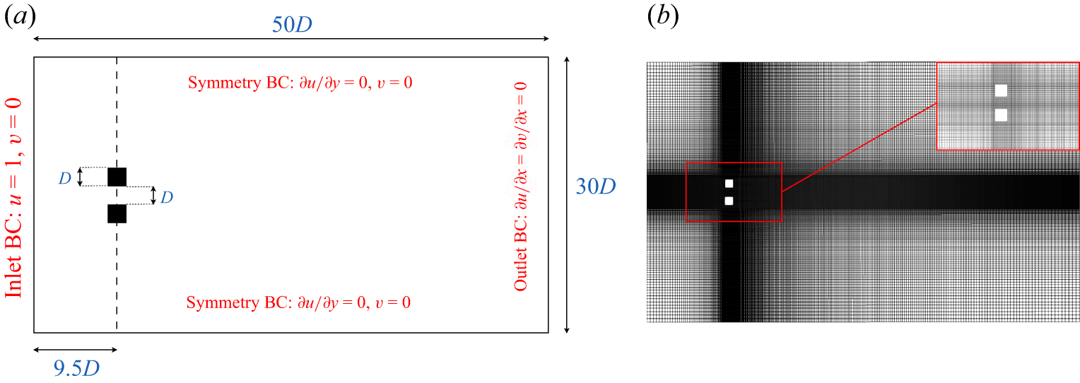
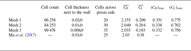


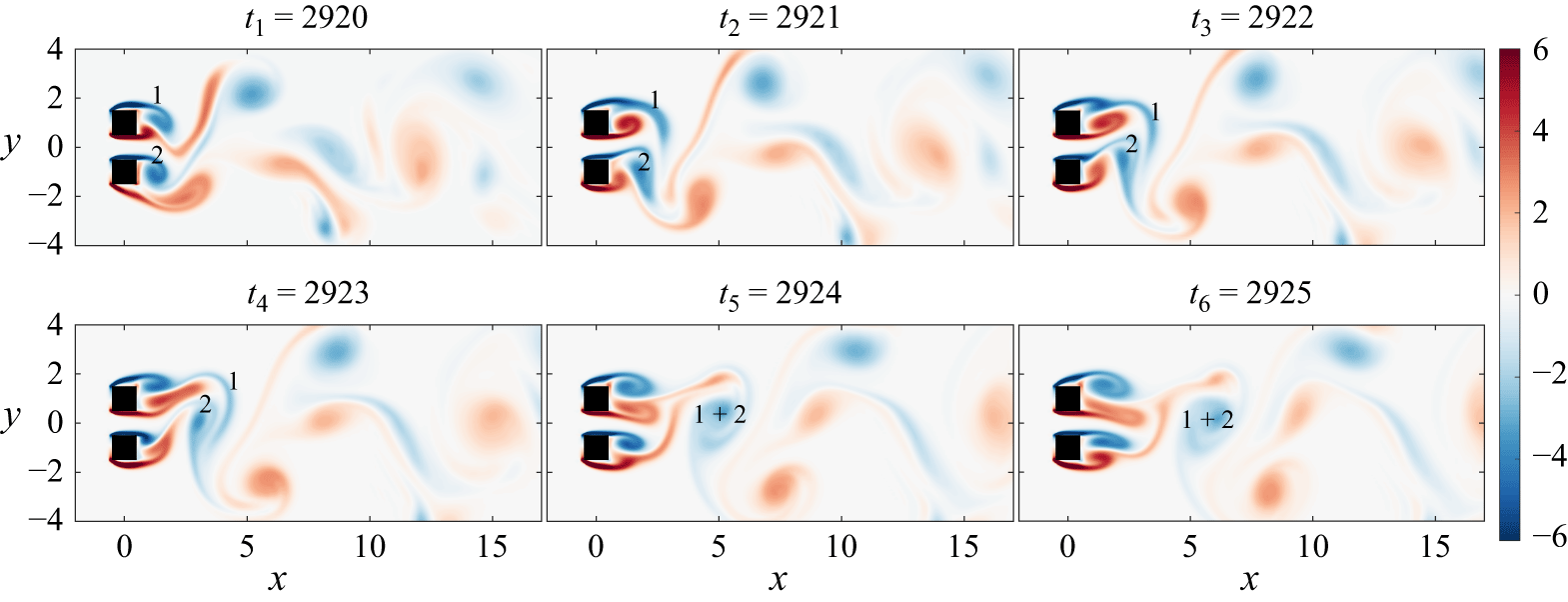

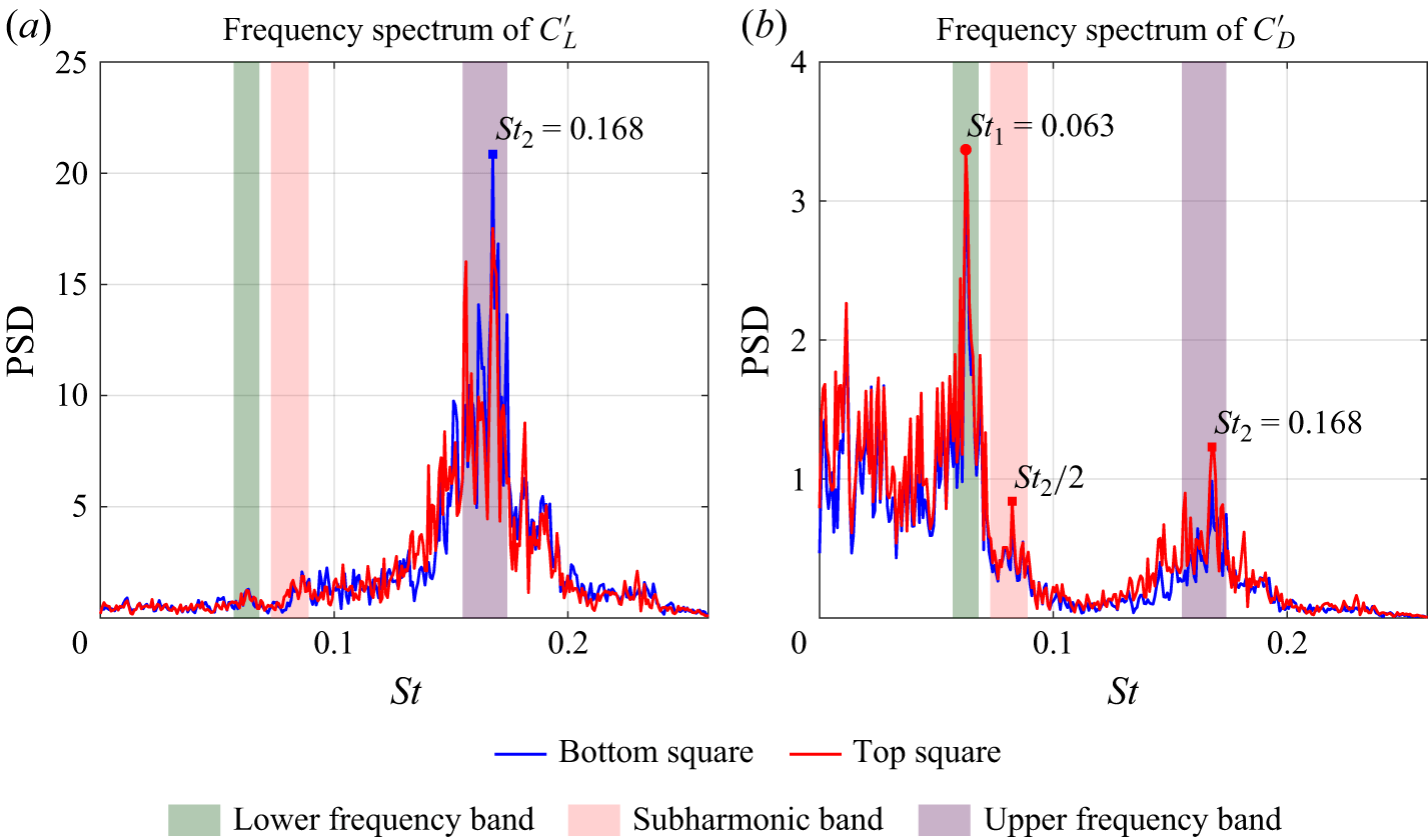


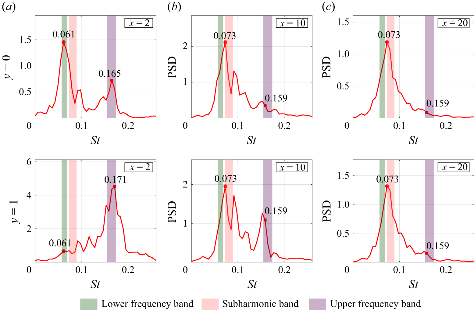


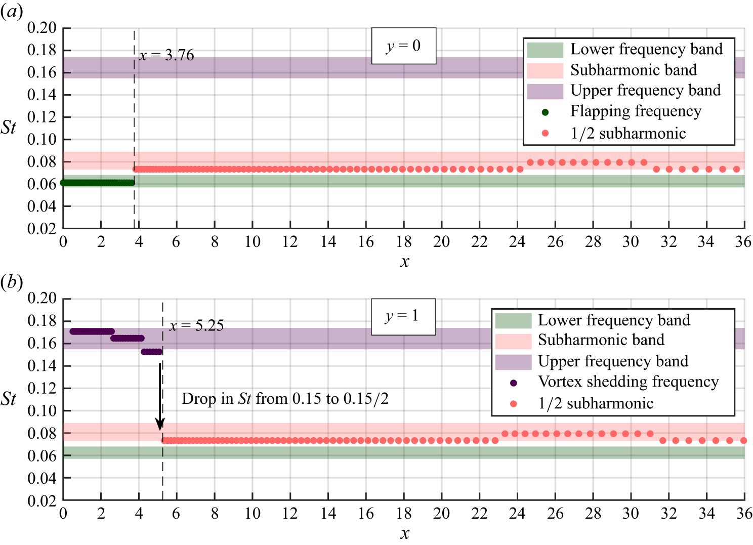


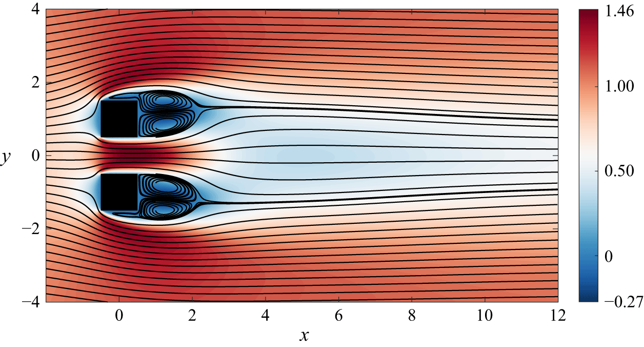

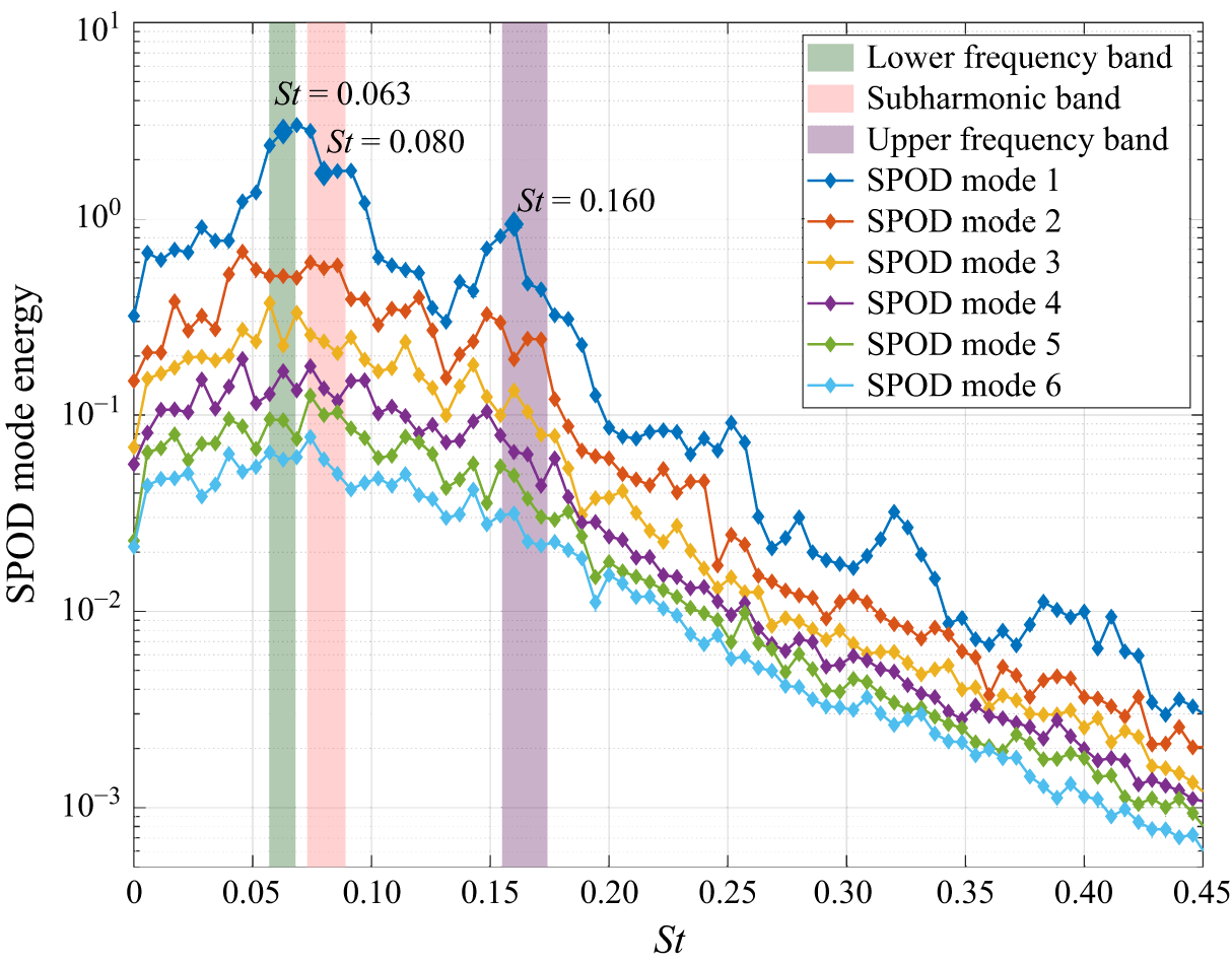
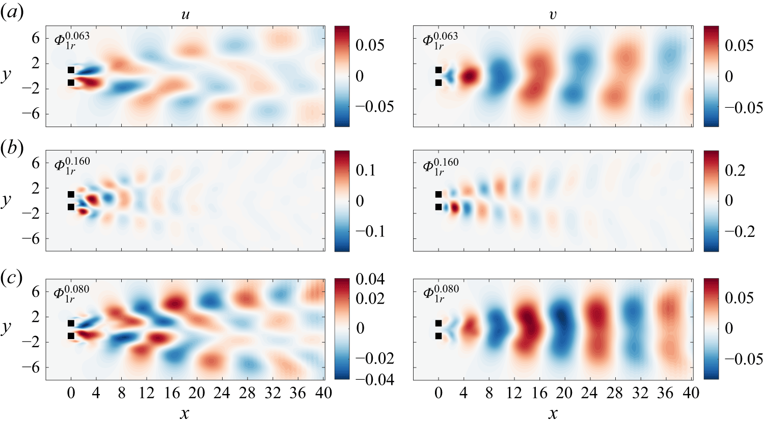


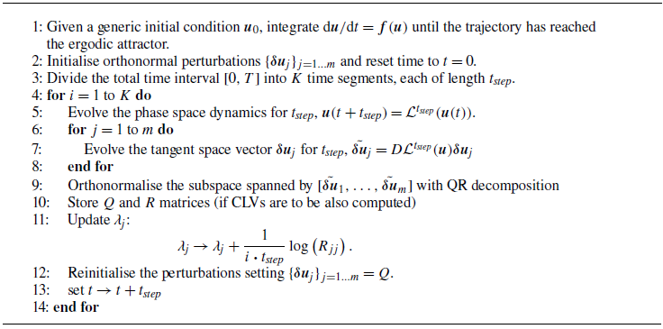
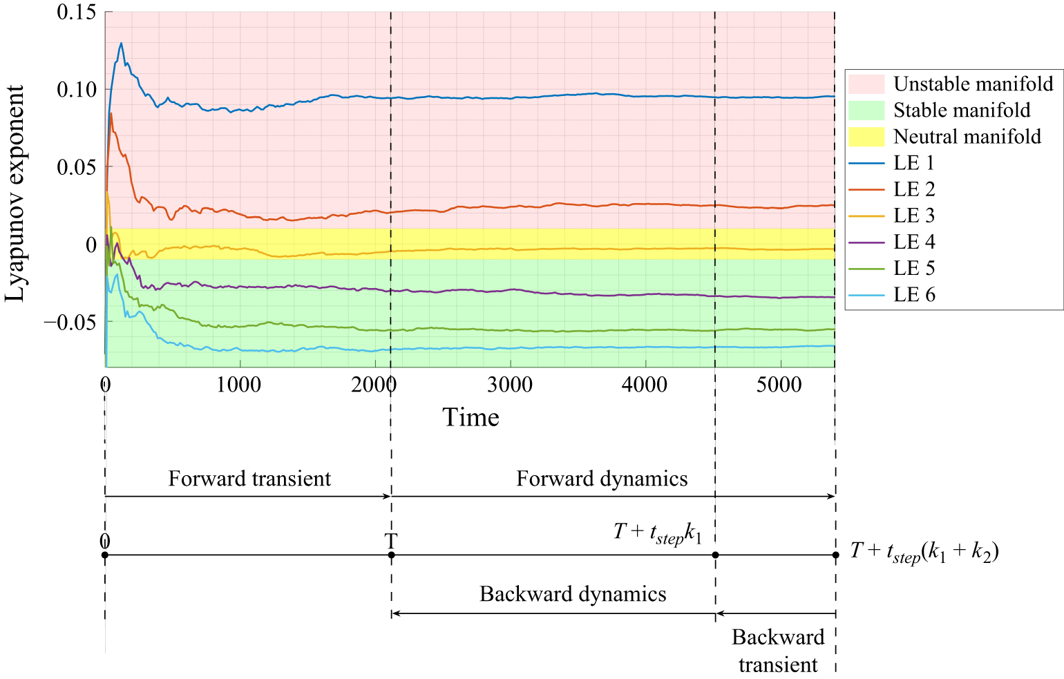

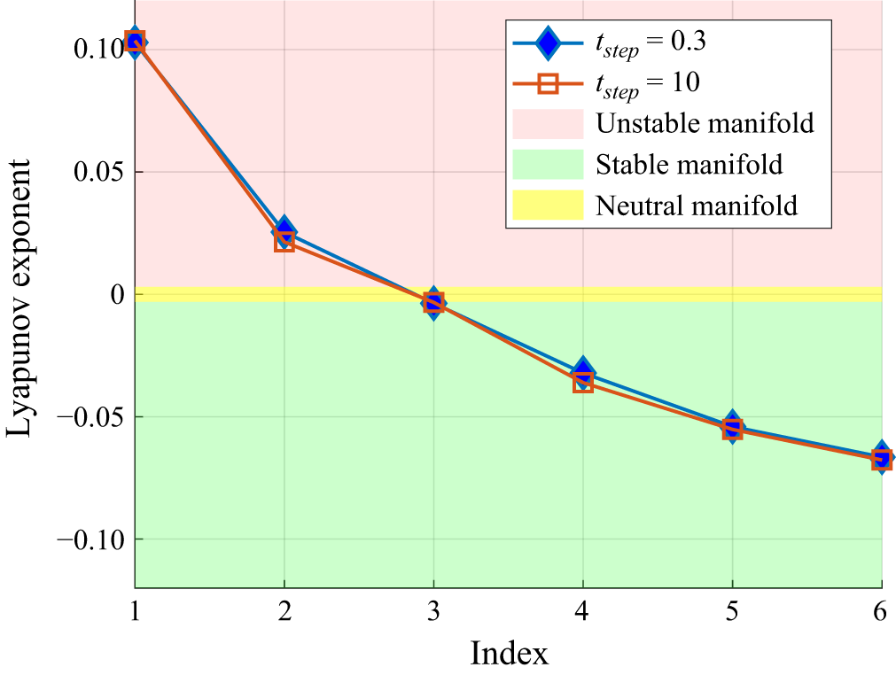
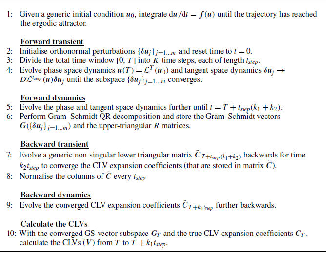
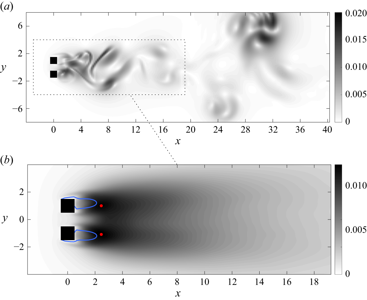


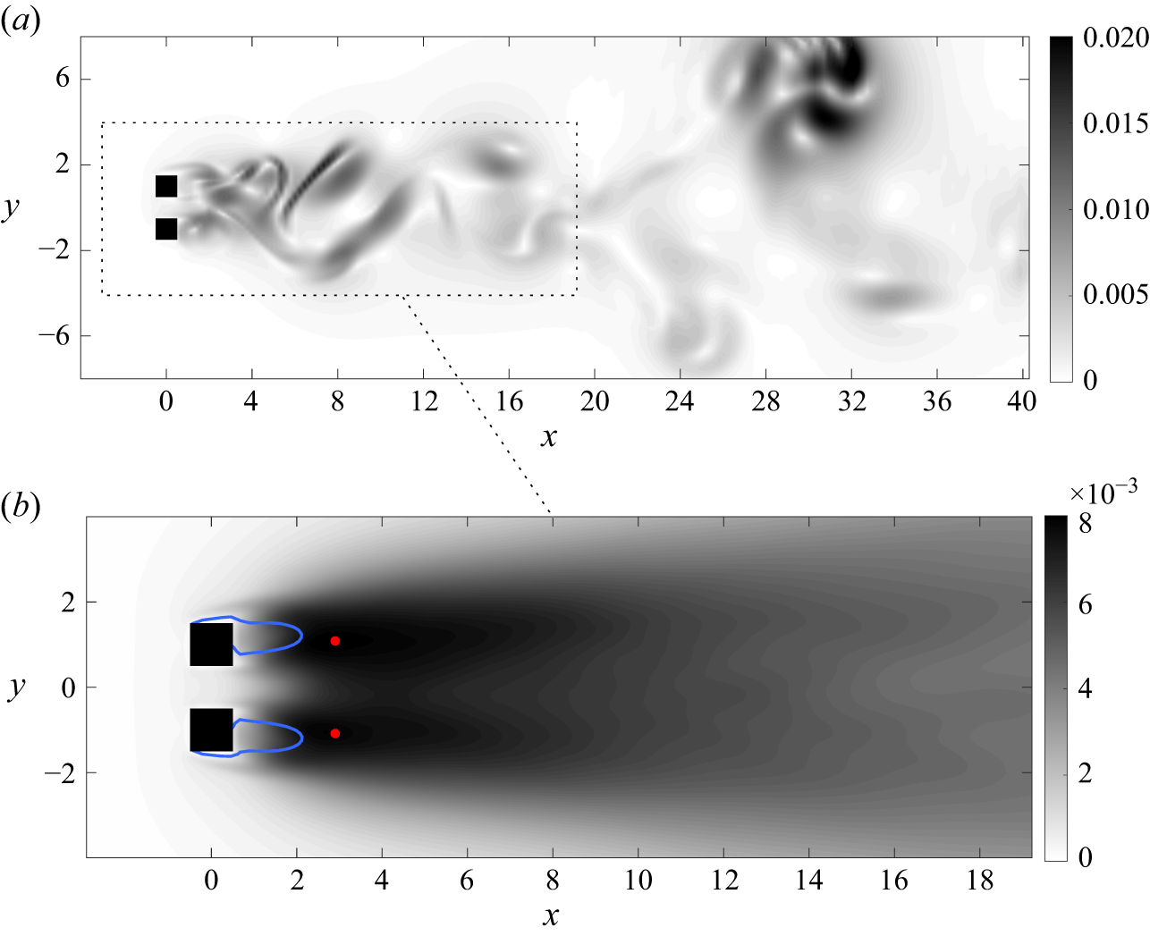


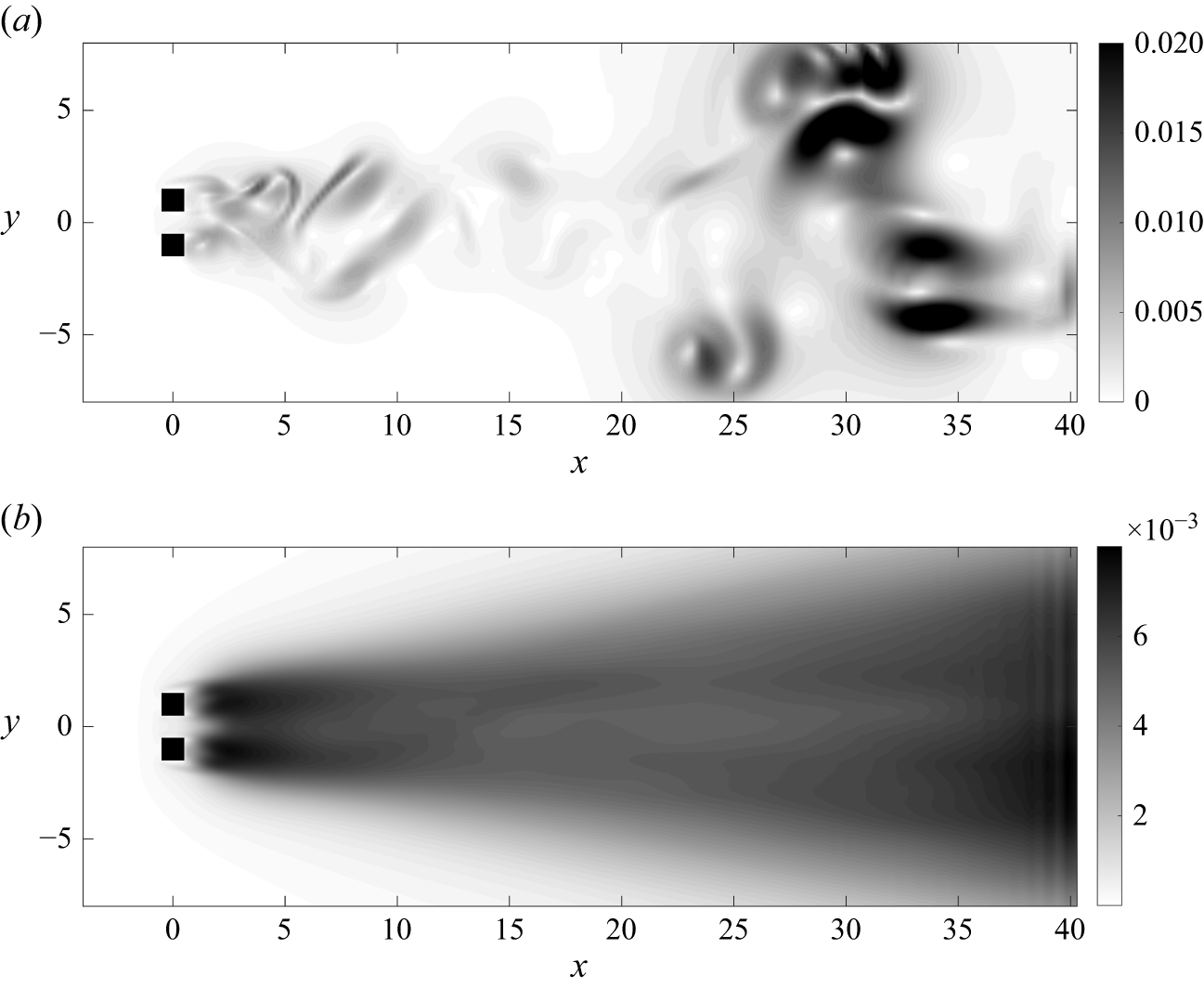


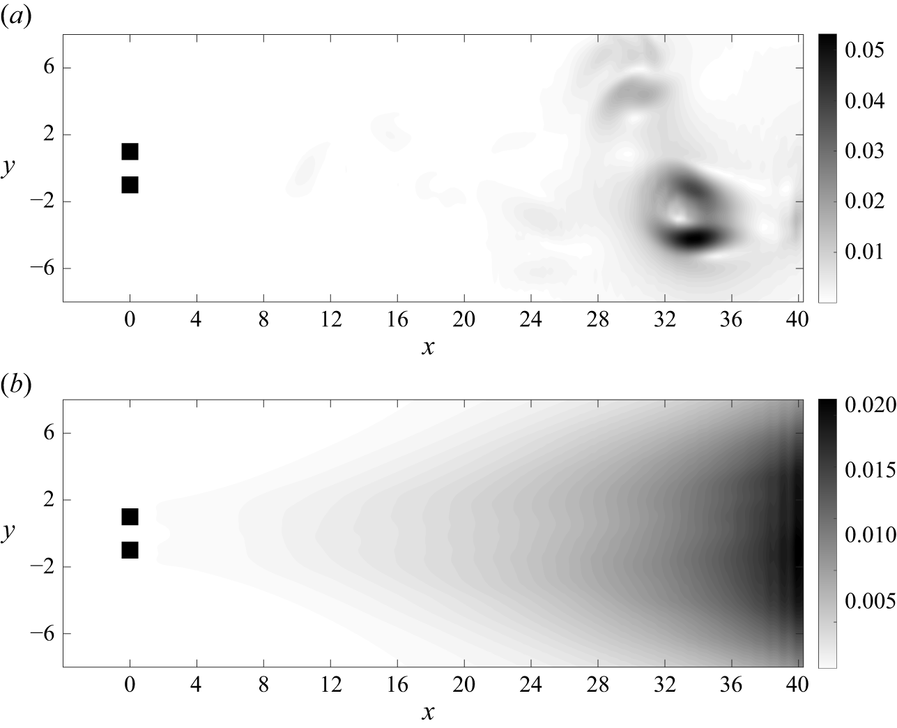


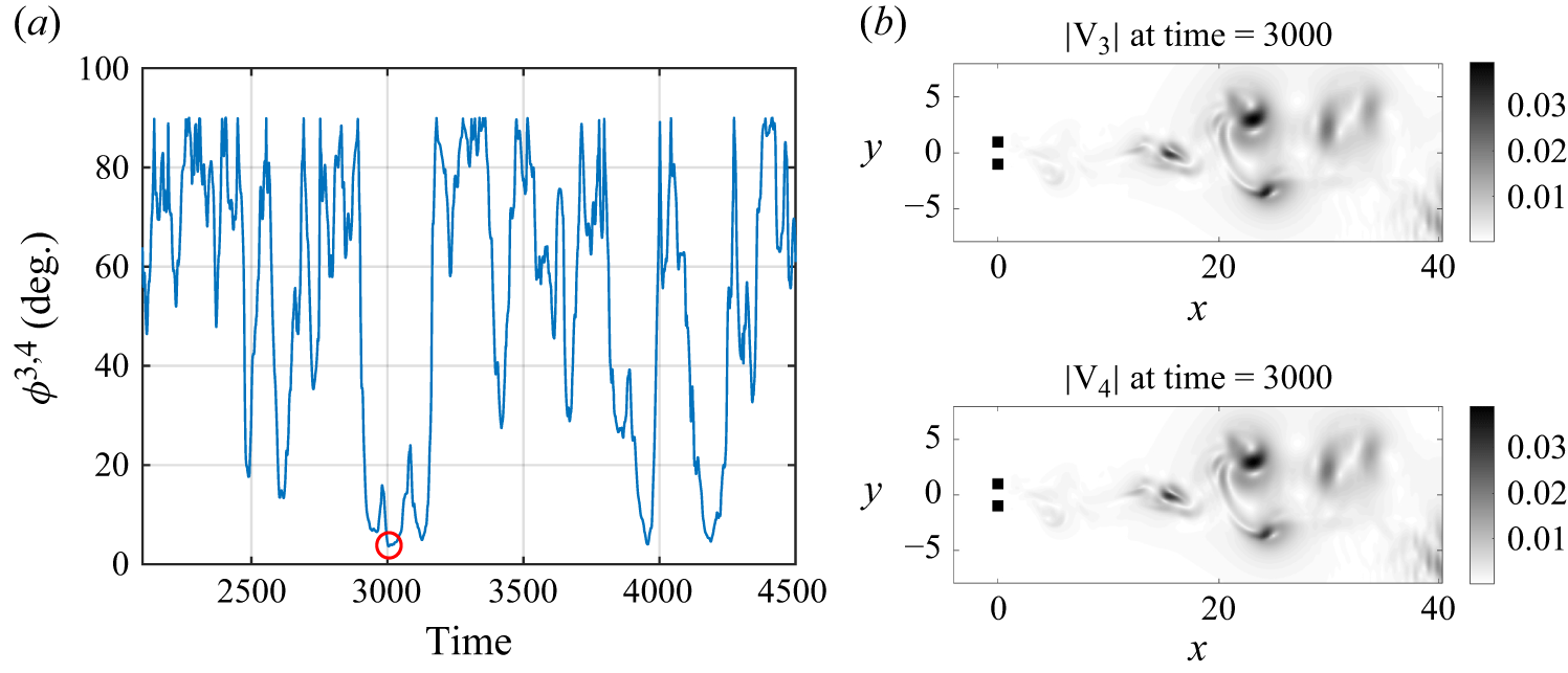


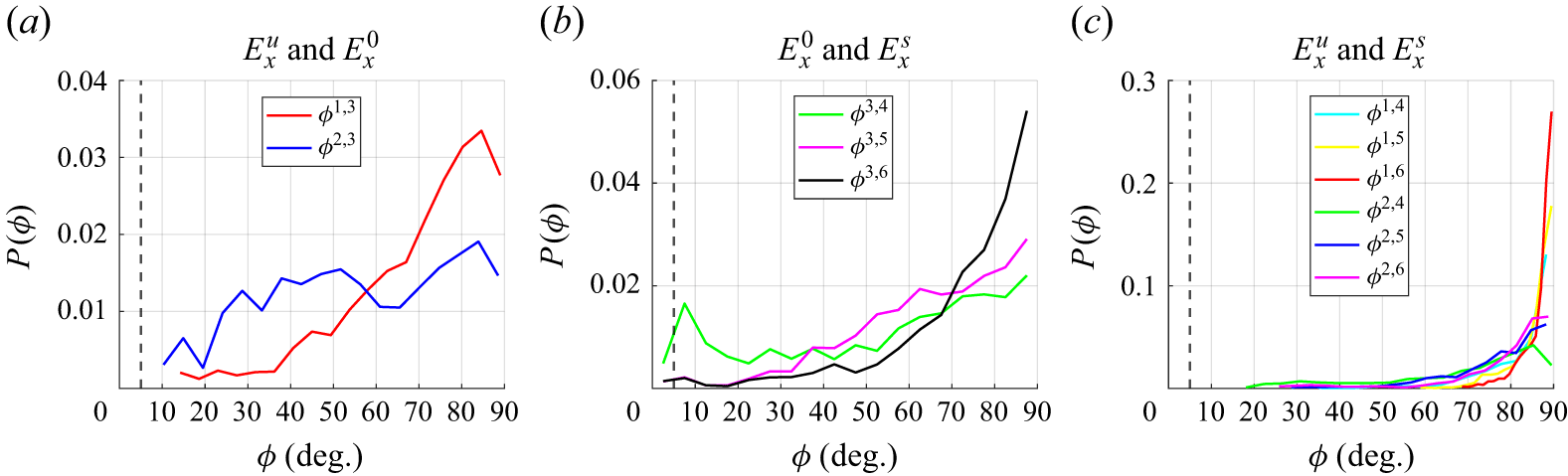

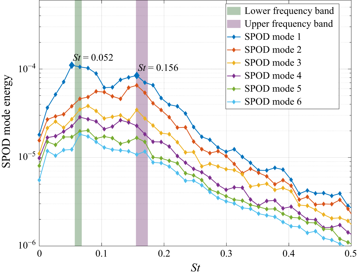

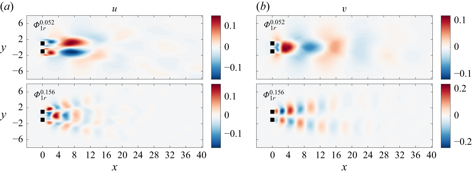


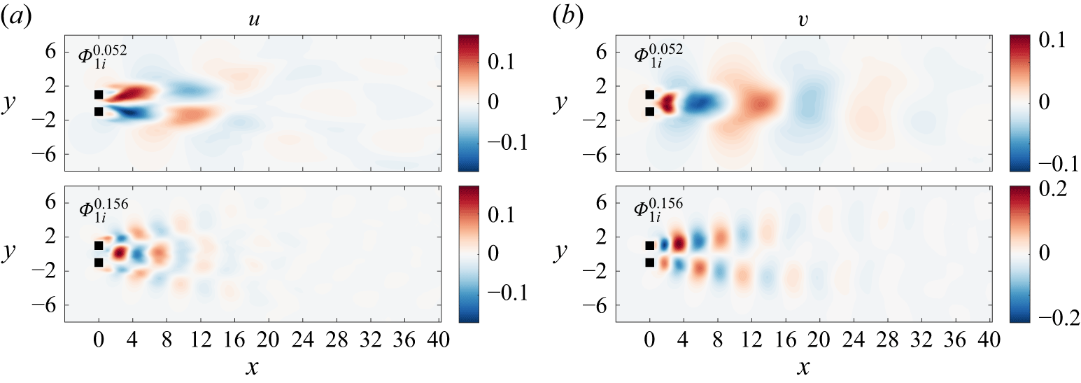


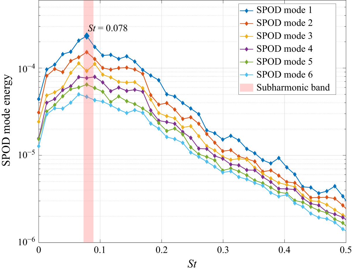

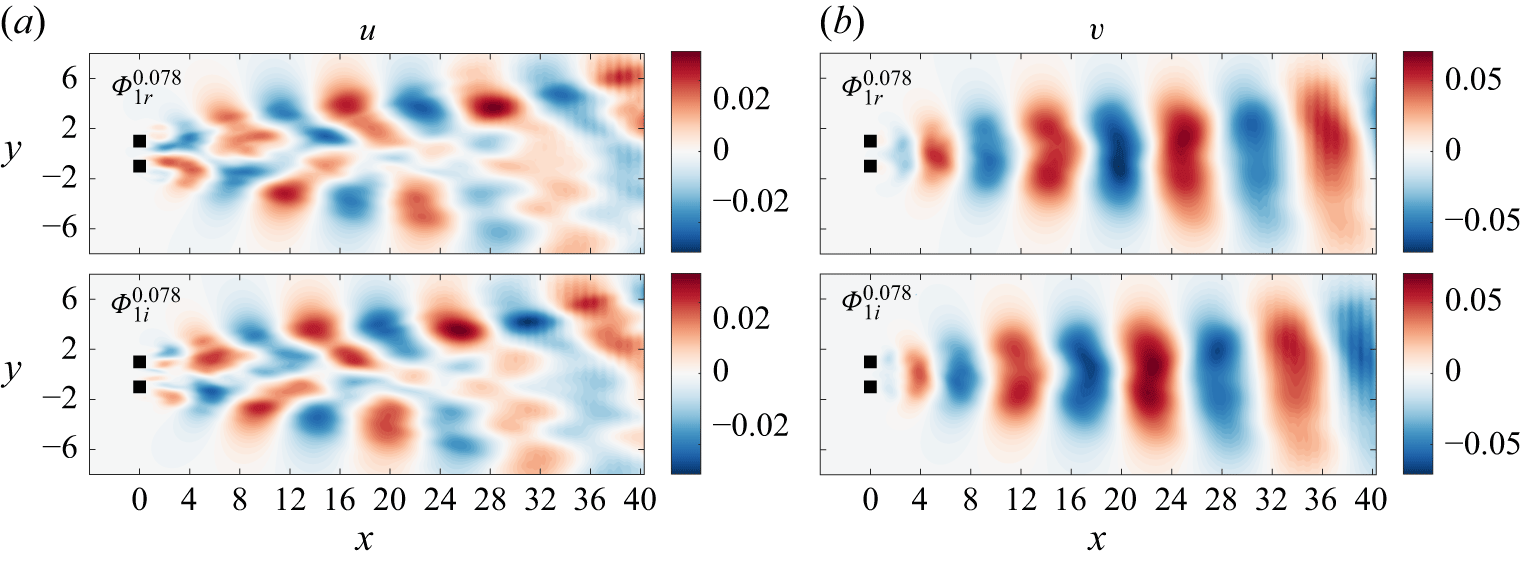


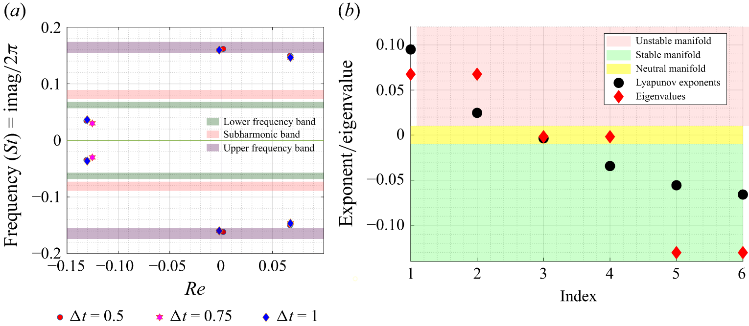
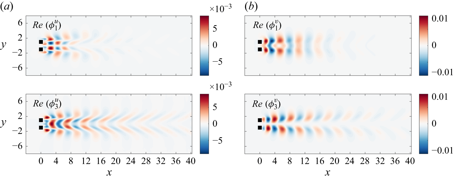


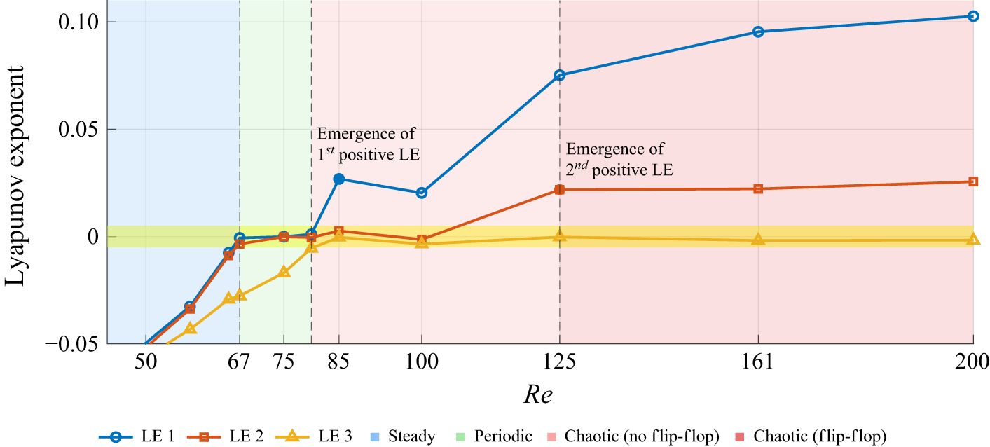


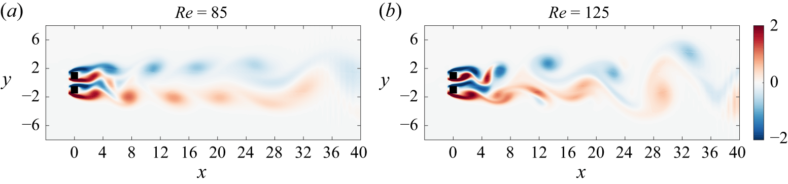


 Open access