


1. Introduction
Phase separation (PS) arises when a homogeneous mixture of partially miscible fluids becomes thermodynamically unstable and divides into distinct phases (Iwasaki et al. Reference Iwasaki, Nagatsu, Ban, Iijima, Mishra and Suzuki2023). It is a widespread phenomenon in both natural systems and technological applications. It plays a key role in processes such as enhanced oil recovery (Lake et al. Reference Lake, Johns, Rossen and Pope2014; Faisal et al. Reference Faisal, Chevalier, Bernabe, Juanes and Sassi2015; Fu et al. Reference Fu, Cueto-Felgueroso, Bolster and Juanes2015), carbon sequestration (Orr Jr. & Taber Reference Orr and Taber1984; Fu, Cueto-Felgueroso & Juanes Reference Fu, Cueto-Felgueroso and Juanes2017; Amooie, Soltanian & Moortgat Reference Amooie, Soltanian and Moortgat2017) and microfluidic technologies (Guo et al. Reference Guo, Cheng, Chen and Chou2023; Chu et al. Reference Chu2023). In particular, CO $_2$
-enhanced oil recovery (CO
$_2$
-enhanced oil recovery (CO $_2$
-EOR) has garnered significant attention as a method to improve oil production, wherein CO
$_2$
-EOR) has garnered significant attention as a method to improve oil production, wherein CO $_2$
is injected into saline aquifers in a supercritical state under high-temperature and high-pressure conditions (Wang et al. Reference Wang, Dong, Li and Gong2015; Zhou et al. Reference Zhou, Yuan, Zhang, Wang, Zeng and Zhang2019; Li et al. Reference Li, Cai, Chen and Meiburg2022). In this state, CO
$_2$
is injected into saline aquifers in a supercritical state under high-temperature and high-pressure conditions (Wang et al. Reference Wang, Dong, Li and Gong2015; Zhou et al. Reference Zhou, Yuan, Zhang, Wang, Zeng and Zhang2019; Li et al. Reference Li, Cai, Chen and Meiburg2022). In this state, CO $_2$
is partially miscible with oil (Huppert & Neufeld Reference Huppert and Neufeld2014). However, the efficiency of this process is often hindered by complex interfacial phenomena, such as viscous fingering (VF) and PS under high-temperature and high-pressure conditions in the particular underground environment (Orr Jr. & Taber Reference Orr and Taber1984; Huppert & Neufeld Reference Huppert and Neufeld2014; Li et al. Reference Li, Lin, Cai, Chen and Meiburg2023). Viscous fingering arises when a less viscous fluid displaces a more viscous one, developing finger-like patterns at the interface (Homsy Reference Homsy1987). This instability can result in inefficient displacement and reduced recovery rates. Traditionally, VF has been studied in the context of fully miscible or immiscible fluids. However, the interplay between thermodynamic (PS) and hydrodynamic (VF) instabilities in partially miscible systems introduces additional complexity. Further, the partially miscible system can be classified depending on whether only one fluid species dissolves into another fluid with finite solubility or both fluid species dissolve into each other and undergo PS to form new phases. The first case typically occurs in carbon capture and storage, where supercritical CO
$_2$
is partially miscible with oil (Huppert & Neufeld Reference Huppert and Neufeld2014). However, the efficiency of this process is often hindered by complex interfacial phenomena, such as viscous fingering (VF) and PS under high-temperature and high-pressure conditions in the particular underground environment (Orr Jr. & Taber Reference Orr and Taber1984; Huppert & Neufeld Reference Huppert and Neufeld2014; Li et al. Reference Li, Lin, Cai, Chen and Meiburg2023). Viscous fingering arises when a less viscous fluid displaces a more viscous one, developing finger-like patterns at the interface (Homsy Reference Homsy1987). This instability can result in inefficient displacement and reduced recovery rates. Traditionally, VF has been studied in the context of fully miscible or immiscible fluids. However, the interplay between thermodynamic (PS) and hydrodynamic (VF) instabilities in partially miscible systems introduces additional complexity. Further, the partially miscible system can be classified depending on whether only one fluid species dissolves into another fluid with finite solubility or both fluid species dissolve into each other and undergo PS to form new phases. The first case typically occurs in carbon capture and storage, where supercritical CO $_2$
is injected into brine-saturated formations, with a solubility of only approximately 5 % (Huppert & Neufeld Reference Huppert and Neufeld2014; Li et al. Reference Li, Cai, Chen and Meiburg2022, Reference Li, Lin, Cai, Chen and Meiburg2023). In the second case, experimental studies using radial Hele-Shaw flow have revealed novel interfacial patterns resulting from the combined effects of VF and PS (Suzuki et al. Reference Suzuki, Nagatsu, Mishra and Ban2020a
,
Reference Suzuki, Takeda, Nagatsu, Mishra and Banb
).
$_2$
is injected into brine-saturated formations, with a solubility of only approximately 5 % (Huppert & Neufeld Reference Huppert and Neufeld2014; Li et al. Reference Li, Cai, Chen and Meiburg2022, Reference Li, Lin, Cai, Chen and Meiburg2023). In the second case, experimental studies using radial Hele-Shaw flow have revealed novel interfacial patterns resulting from the combined effects of VF and PS (Suzuki et al. Reference Suzuki, Nagatsu, Mishra and Ban2020a
,
Reference Suzuki, Takeda, Nagatsu, Mishra and Banb
).
In partially miscible systems, an initial regime characterised by non-Fickian subdiffusive spreading is identified, distinguishing it from the diffusive mixing behaviour typically observed in fully miscible systems (Amooie et al. Reference Amooie, Soltanian and Moortgat2017). Further, Fu, Cueto-Felgueroso & Juanes (Reference Fu, Cueto-Felgueroso and Juanes2016) conducted numerical analyses demonstrating that VF significantly influences the PS dynamics. It leads to phase branching and tip splitting, destabilising the leading edges of gas bubbles and inducing pinch-off events. Beyond numerical investigations, several experimental studies have been dedicated to understanding the nonlinear interaction between VF and PS in partially miscible systems. These experiments commonly utilise aqueous two-phase systems (ATPSs), consisting of polyethylene glycol (PEG) solutions and sodium sulphate (Na $_2$
SO
$_2$
SO $_4$
), to represent more and less viscous fluids, respectively. Different combinations of fluid concentrations and experimental set-ups have been employed to explore a range of flow conditions. For instance, Suzuki et al. (Reference Suzuki, Nagatsu, Mishra and Ban2019) investigated the displacement of the less viscous fluid PEG by the more viscous Na
$_4$
), to represent more and less viscous fluids, respectively. Different combinations of fluid concentrations and experimental set-ups have been employed to explore a range of flow conditions. For instance, Suzuki et al. (Reference Suzuki, Nagatsu, Mishra and Ban2019) investigated the displacement of the less viscous fluid PEG by the more viscous Na $_2$
SO
$_2$
SO $_4$
, focusing on fingering dynamics driven by spinodal decomposition. In this process, a thermodynamically unstable mixture spontaneously separates into two distinct phases. By varying the concentration of components in ATPS, they examined systems ranging from fully miscible to partially miscible or immiscible. For example, a fully miscible system was represented by 36.5 % PEG and 0 % Na
$_4$
, focusing on fingering dynamics driven by spinodal decomposition. In this process, a thermodynamically unstable mixture spontaneously separates into two distinct phases. By varying the concentration of components in ATPS, they examined systems ranging from fully miscible to partially miscible or immiscible. For example, a fully miscible system was represented by 36.5 % PEG and 0 % Na $_2$
SO
$_2$
SO $_4$
, while a partially miscible one used 36.5 % PEG and 20 % Na
$_4$
, while a partially miscible one used 36.5 % PEG and 20 % Na $_2$
SO
$_2$
SO $_4$
. They found that the interfacial tension remains constant over time for immiscible fluids and decays to zero for fully miscible fluids. While for partially miscible fluids, it increases and then saturates, with the saturated value higher than in immiscible cases. In a follow-up study, Suzuki et al. (Reference Suzuki, Takeda, Nagatsu, Mishra and Ban2020b
) extended their analysis to explore the fluid morphologies resulting from PS-induced VF in hydrodynamically stable flow. They observed that the instability pattern depends on the concentration of the injected fluid, while the concentration of the displaced fluid determines the miscibility of the system. For Na
$_4$
. They found that the interfacial tension remains constant over time for immiscible fluids and decays to zero for fully miscible fluids. While for partially miscible fluids, it increases and then saturates, with the saturated value higher than in immiscible cases. In a follow-up study, Suzuki et al. (Reference Suzuki, Takeda, Nagatsu, Mishra and Ban2020b
) extended their analysis to explore the fluid morphologies resulting from PS-induced VF in hydrodynamically stable flow. They observed that the instability pattern depends on the concentration of the injected fluid, while the concentration of the displaced fluid determines the miscibility of the system. For Na $_2$
SO
$_2$
SO $_4$
concentrations below 9 %, a stable circular region was observed regardless of PEG concentration. However, when Na
$_4$
concentrations below 9 %, a stable circular region was observed regardless of PEG concentration. However, when Na $_2$
SO
$_2$
SO $_4$
and PEG concentrations ranged between 10 %–20 % and 10 %–35 %, respectively, annular or fingering patterns emerged depending on the specific concentration combinations. We discuss the results of this study in detail in § 3.4.
$_4$
and PEG concentrations ranged between 10 %–20 % and 10 %–35 %, respectively, annular or fingering patterns emerged depending on the specific concentration combinations. We discuss the results of this study in detail in § 3.4.
Further, Suzuki et al. (Reference Suzuki, Nagatsu, Mishra and Ban2020a ) investigated the effects of PS on VF by examining the displacement of a more viscous fluid by a less viscous one. Through nonlinear simulations and experiments, they demonstrated that, in partially miscible systems, the anomalous finger formation transitions into generating spontaneously moving multiple droplets under this flow configuration. However, the numerical studies exploring PS effects were mostly conducted within a rectilinear flow geometry (Seya et al. Reference Seya, Suzuki, Nagatsu, Ban and Mishra2022; Kim et al. Reference Kim, Palodhi, Hong and Mishra2023). Subsequently, Deki et al. (Reference Deki, Suzuki, Chou, Ban, Mishra, Nagatsu and Chen2025) performed numerical simulations in a radial flow geometry for the same scenario, where a less viscous fluid displaces a more viscous one. Employing the Hele-Shaw–Cahn–Hilliard model, they numerically obtained the anomalous fingering patterns observed in experiments (Suzuki et al. Reference Suzuki, Nagatsu, Mishra and Ban2020a ), specifically, the tip-widening (or lollipop) fingers with slim stems and droplets, resulting from the interplay between thermodynamic (PS) and hydrodynamic (VF) instabilities (Suzuki et al. Reference Suzuki, Tada, Hirano, Ban, Mishra, Takeda and Nagatsu2021). Despite these advances, an independent analysis of PS in a hydrodynamically stable displacement in the absence of VF influence remains unexplored. Notably, how PS can induce VF in hydrodynamically stable situations where a more viscous fluid displaces a less viscous fluid, as experimentally shown by Suzuki et al. (Reference Suzuki, Nagatsu, Mishra and Ban2019, Reference Suzuki, Takeda, Nagatsu, Mishra and Ban2020b ), has yet to be thoroughly investigated. In this study, we investigate the coupled effects of VF and PS in a radial Hele-Shaw cell for the hydrodynamically stable where PS may induce the VF. By conducting nonlinear simulations, we aim to elucidate the mechanisms governing pattern formation and the onset of instability in partially miscible displacements. Our findings provide insights into the conditions that favour or suppress instabilities, offering guidance for improving fluid displacement strategies in practical applications.
The organisation of the paper is as follows: § 2 presents the mathematical formulation and details the numerical scheme employed for nonlinear simulations. In § 3, we discuss the results obtained from these simulations. Finally, § 4 provides a conclusion of our findings.
2. Mathematical formulation
We consider displacement in a radial Hele-Shaw cell involving two fluids. Both fluids are Newtonian and incompressible. The phase variable $c$
, representing the mass fraction or concentration in this model, is defined such that
$c$
, representing the mass fraction or concentration in this model, is defined such that $c = 1$
corresponds to the fluid with viscosity
$c = 1$
corresponds to the fluid with viscosity ${\eta }_1$
, and
${\eta }_1$
, and $c = 0$
to the fluid with viscosity
$c = 0$
to the fluid with viscosity ${\eta }_2$
. The concentrations of the injected and displaced fluids are denoted by
${\eta }_2$
. The concentrations of the injected and displaced fluids are denoted by $c_i$
and
$c_i$
and $c_0$
, respectively, with
$c_0$
, respectively, with $c_i \leqslant 1$
and
$c_i \leqslant 1$
and $c_0 = 0$
. A flow schematic is presented in figure 1(
$c_0 = 0$
. A flow schematic is presented in figure 1( $a$
), illustrating an unstable displacement driven by intrinsic thermodynamic and induced hydrodynamic instabilities. To model partial miscibility in a binary system, we assume a symmetric miscibility profile as miscibility
$a$
), illustrating an unstable displacement driven by intrinsic thermodynamic and induced hydrodynamic instabilities. To model partial miscibility in a binary system, we assume a symmetric miscibility profile as miscibility $c_{s1} = c_s$
, so the complementary miscibility is
$c_{s1} = c_s$
, so the complementary miscibility is $c_{s2} = 1- c_s$
(Deki et al. Reference Deki, Suzuki, Chou, Ban, Mishra, Nagatsu and Chen2025). When
$c_{s2} = 1- c_s$
(Deki et al. Reference Deki, Suzuki, Chou, Ban, Mishra, Nagatsu and Chen2025). When $c_s = 0$
and the initial condition is
$c_s = 0$
and the initial condition is $(c_i, c_0) = (1, 0)$
, the system represents a fully immiscible flow (Chen et al. Reference Chen, Huang and Miranda2011, Reference Chen, Huang and Miranda2014; Tsuzuki et al. Reference Tsuzuki, Li, Nagatsu and Chen2019). The governing equations for the diffuse-interface approach in non-dimensionalised form are given as follows (Chen, Huang & Miranda Reference Chen, Huang and Miranda2011; Deki et al. Reference Deki, Suzuki, Chou, Ban, Mishra, Nagatsu and Chen2025):
$(c_i, c_0) = (1, 0)$
, the system represents a fully immiscible flow (Chen et al. Reference Chen, Huang and Miranda2011, Reference Chen, Huang and Miranda2014; Tsuzuki et al. Reference Tsuzuki, Li, Nagatsu and Chen2019). The governing equations for the diffuse-interface approach in non-dimensionalised form are given as follows (Chen, Huang & Miranda Reference Chen, Huang and Miranda2011; Deki et al. Reference Deki, Suzuki, Chou, Ban, Mishra, Nagatsu and Chen2025):
 \begin{align}&\qquad\qquad\qquad \boldsymbol{\nabla } \boldsymbol{\cdot }\boldsymbol{u}=0 , \end{align}
 \begin{align}&\qquad \boldsymbol{\nabla }\! p=-\eta \boldsymbol{u} - \frac {C}{I}\bigl[(\boldsymbol{\nabla } c) \times (\boldsymbol{\nabla } c)^T \bigr] , \end{align}
 \begin{align}&\qquad\qquad \dfrac {\partial c}{\partial t}+\boldsymbol{u} \boldsymbol{\cdot }\boldsymbol{\nabla }c=\frac {1}{\textit{Pe}}{\nabla} ^2 \mu , \end{align}
 \begin{align}& \mu =\frac {{\rm d}f}{{\rm d}c}-C{\nabla} ^2 c, \quad f=(c-c_{s1})^2(c-c_{s2})^2, \end{align}
 \begin{align}&\qquad\quad \eta (c)=e^{R(1-\textit{c})}, \quad R=\ln \bigg (\dfrac {{\eta }_2 }{{\eta }_1}\bigg ), \end{align}

Figure 1. ( $a$
) Schematic of the computational domain
$a$
) Schematic of the computational domain $\varOmega =[-1,1] \times [-1,1]$
for the simulations. The inner circle of radius
$\varOmega =[-1,1] \times [-1,1]$
for the simulations. The inner circle of radius $R_i$
, the core region, contains injected fluid with a concentration
$R_i$
, the core region, contains injected fluid with a concentration $c=c_i$
, while the outer region beyond the circle in dashed lines is occupied by displaced fluid with a concentration
$c=c_i$
, while the outer region beyond the circle in dashed lines is occupied by displaced fluid with a concentration $c=c_0$
. In the annular region between these two circles, instabilities manifest as droplets, rings and fingering patterns. Within the droplets, the concentration reaches either miscibility (
$c=c_0$
. In the annular region between these two circles, instabilities manifest as droplets, rings and fingering patterns. Within the droplets, the concentration reaches either miscibility ( $c=c_s$
) or complementary miscibility
$c=c_s$
) or complementary miscibility $c=1-c_s$
. (
$c=1-c_s$
. ( $b$
) A schematic illustrating different zones in the concentration profile along the centreline
$b$
) A schematic illustrating different zones in the concentration profile along the centreline $(y = 0)$
, where
$(y = 0)$
, where $\mathcal{C}_r$
,
$\mathcal{C}_r$
, $\mathcal{S}$
and
$\mathcal{S}$
and $\varOmega _1$
represent the core region, spinodal decomposition and fully separated region, respectively. The representative case for both figures is the results for
$\varOmega _1$
represent the core region, spinodal decomposition and fully separated region, respectively. The representative case for both figures is the results for $R=-3$
,
$R=-3$
, $c_i=0.5$
, and
$c_i=0.5$
, and $c_s=0$
.
$c_s=0$
.
where $\boldsymbol{u}= (u,v)$
,
$\boldsymbol{u}= (u,v)$
, $p$
,
$p$
, $\mu$
and
$\mu$
and $f$
denote the Darcy velocity, pressure, chemical potential of the phase and Helmholtz free energy, respectively. The effect of density difference on the VF and PS can be ignored Suzuki et al. (Reference Suzuki, Nagatsu, Mishra and Ban2020a
); as a result, a constant density is taken in the model. To non-dimensionalise the governing equations, we consider
$f$
denote the Darcy velocity, pressure, chemical potential of the phase and Helmholtz free energy, respectively. The effect of density difference on the VF and PS can be ignored Suzuki et al. (Reference Suzuki, Nagatsu, Mishra and Ban2020a
); as a result, a constant density is taken in the model. To non-dimensionalise the governing equations, we consider $2r_c$
as the characteristic length scale and
$2r_c$
as the characteristic length scale and $t_c$
as the characteristic time, which is the time required to expand injected fluid to the radius of
$t_c$
as the characteristic time, which is the time required to expand injected fluid to the radius of $r_c$
in the absence of viscosity contrast. The viscosity, free energy, Darcy velocity and pressure are non-dimensionalised by
$r_c$
in the absence of viscosity contrast. The viscosity, free energy, Darcy velocity and pressure are non-dimensionalised by $\eta _1$
, characteristic free energy (
$\eta _1$
, characteristic free energy ( $f_0$
),
$f_0$
), $2r_c/t_c$
and
$2r_c/t_c$
and $48 \eta _1 r_c^2 / b^2 t_c$
, respectively.
$48 \eta _1 r_c^2 / b^2 t_c$
, respectively.
In (2.1e
), we consider viscosity to be dependent on concentration exponentially (Chen & Meiburg Reference Chen and Meiburg1998; Sharma et al. Reference Sharma, Nand, Pramanik, Chen and Mishra2020). Here, $R$
characterises the log-mobility ratio between the displacing and displaced fluids:
$R$
characterises the log-mobility ratio between the displacing and displaced fluids: $R\gt 0$
corresponds to a hydrodynamically unstable flow where a less viscous fluid displaces a more viscous one. In this study, we focus on hydrodynamically stable conditions with
$R\gt 0$
corresponds to a hydrodynamically unstable flow where a less viscous fluid displaces a more viscous one. In this study, we focus on hydrodynamically stable conditions with $R\leqslant 0$
. Nevertheless, VF can be induced by a thermodynamic instability. Other than
$R\leqslant 0$
. Nevertheless, VF can be induced by a thermodynamic instability. Other than $ R $
, we have three dimensionless parameters: Péclet number (
$ R $
, we have three dimensionless parameters: Péclet number ( $\textit{Pe}$
), Cahn number (
$\textit{Pe}$
), Cahn number ( $C$
) and injection parameter (
$C$
) and injection parameter ( $I$
) as follows:
$I$
) as follows:
 \begin{align} {\textit{Pe}}=\dfrac {4 {\rho }{r}^2_c }{{\alpha }{f}_0{t}_c }, \quad C=\dfrac {{\epsilon }}{ 4 {r}^2_c {f}_0 }, \quad I=\dfrac {48 {\eta }_1 {r}^2_c }{ {b}^2{\rho } {f}_0 {t}_c }. \end{align}
Here, the Péclet number ( $Pe$
) determines dissipation in the flow. The Cahn number (
$Pe$
) determines dissipation in the flow. The Cahn number ( $C$
) and the injection parameter (
$C$
) and the injection parameter ( $I$
) are both linked to interfacial tension, with lower values of
$I$
) are both linked to interfacial tension, with lower values of $C$
and a larger value of
$C$
and a larger value of $I$
corresponding to stronger interfacial tension (Deki et al. Reference Deki, Suzuki, Chou, Ban, Mishra, Nagatsu and Chen2025). Meanwhile, the value of
$I$
corresponding to stronger interfacial tension (Deki et al. Reference Deki, Suzuki, Chou, Ban, Mishra, Nagatsu and Chen2025). Meanwhile, the value of $C$
governs the effective thickness of the diffuse interface in the model (Lowengrub & Truskinovsky Reference Lowengrub and Truskinovsky1998; Li et al. Reference Li, Cai, Chen and Meiburg2022). Further,
$C$
governs the effective thickness of the diffuse interface in the model (Lowengrub & Truskinovsky Reference Lowengrub and Truskinovsky1998; Li et al. Reference Li, Cai, Chen and Meiburg2022). Further, $\rho$
,
$\rho$
, $\alpha$
,
$\alpha$
, $\epsilon$
and
$\epsilon$
and $b$
stand for density, coefficient of mobility, coefficient of capillary and gap width of the Hele-Shaw cell, respectively. The associated initial conditions for concentration are
$b$
stand for density, coefficient of mobility, coefficient of capillary and gap width of the Hele-Shaw cell, respectively. The associated initial conditions for concentration are
 \begin{equation} c(\boldsymbol{x}, t=0)=\begin{cases} c_i, \quad r \leqslant r_0, \\0, \,\quad r \gt r_0, \end{cases} \end{equation}
where $r=\sqrt {x^2+y^2}$
,
$r=\sqrt {x^2+y^2}$
, $\boldsymbol{x}=(x,y)$
and
$\boldsymbol{x}=(x,y)$
and $r_0$
is the dimensionless radius of the injection hole. To simulate the flow and interfacial dynamics, we adopt the numerical approach successfully applied to similar problems where PS effects on VF were investigated for the cases
$r_0$
is the dimensionless radius of the injection hole. To simulate the flow and interfacial dynamics, we adopt the numerical approach successfully applied to similar problems where PS effects on VF were investigated for the cases $R\geqslant 0$
by Deki et al. (Reference Deki, Suzuki, Chou, Ban, Mishra, Nagatsu and Chen2025) and Liao, Verma & Chen (Reference Liao, Verma and Chen2025). A detailed description of the algorithm and discretisation is provided in § 2.1.
$R\geqslant 0$
by Deki et al. (Reference Deki, Suzuki, Chou, Ban, Mishra, Nagatsu and Chen2025) and Liao, Verma & Chen (Reference Liao, Verma and Chen2025). A detailed description of the algorithm and discretisation is provided in § 2.1.
2.1. Numerical method for nonlinear simulations
We perform numerical computations in Cartesian coordinates on a square computational domain, $\varOmega =[-1,1] \times [-1,1]$
discretised uniformly using a 1025
$\varOmega =[-1,1] \times [-1,1]$
discretised uniformly using a 1025 $\times$
1025 grid. The total velocity field comprises two components: potential velocity and rotational velocity. The potential velocity results from a source-driven radial flow by an injection strength
$\times$
1025 grid. The total velocity field comprises two components: potential velocity and rotational velocity. The potential velocity results from a source-driven radial flow by an injection strength $Q$
, as follows:
$Q$
, as follows:
 \begin{align} \boldsymbol{u}_{\textit{pot}}=\frac { Q}{ 2 \pi r}\boldsymbol{r}, \quad Q=\frac {\pi \left(1-4r_0^2\right)}{4}. \end{align}
Here, $\boldsymbol{r}$
represents the unit vector along the radial direction. For an ideal source flow, the flow is potential. So that this component is termed as a potential part and satisfies the Laplace equation, i.e. no vorticity is generated. On the other hand, the vorticity is generated by viscosity contrast on the interface, so that this component is termed the rotational part. The total velocity is the sum of these two parts i.e.
$\boldsymbol{r}$
represents the unit vector along the radial direction. For an ideal source flow, the flow is potential. So that this component is termed as a potential part and satisfies the Laplace equation, i.e. no vorticity is generated. On the other hand, the vorticity is generated by viscosity contrast on the interface, so that this component is termed the rotational part. The total velocity is the sum of these two parts i.e. $\boldsymbol{u}=\boldsymbol{u}_{\textit{pot}}+\boldsymbol{u}_{\textit{rot}}$
and is used in the vorticity equation and phase equations. To evaluate the rotational part, we reformulate the governing continuity and momentum equations into the streamfunction–vorticity (
$\boldsymbol{u}=\boldsymbol{u}_{\textit{pot}}+\boldsymbol{u}_{\textit{rot}}$
and is used in the vorticity equation and phase equations. To evaluate the rotational part, we reformulate the governing continuity and momentum equations into the streamfunction–vorticity ( $\psi -\omega$
) formulation as follows:
$\psi -\omega$
) formulation as follows:
 \begin{align}&\qquad\qquad {\nabla} ^2 \psi =-\omega ; \quad (u_{\textit{rot}},v_{\textit{rot}})= \left ( \frac {\partial \psi }{\partial y}, \, -\frac {\partial \psi }{\partial x} \right )\! ,\end{align}
 \begin{align}& \omega =-R \left (u\frac {\partial c}{\partial y} -v\frac {\partial c}{\partial x} \right ) + \frac {C}{\eta I} \bigg (\frac {\partial c}{\partial x} \frac {\partial }{\partial y} ({\nabla} ^2c) - \frac {\partial c}{\partial y} \frac {\partial }{\partial x} ({\nabla} ^2c)\bigg ) . \end{align}
Since the potential velocity exhibits a singularity at the origin, we regularise it using a Gaussian source core of width $\sigma \leqslant r_0$
, following the approach of Chen et al. (Reference Chen, Huang, Gadêlha and Miranda2008) and Sharma et al. (Reference Sharma, Pramanik, Chen and Mishra2019)
$\sigma \leqslant r_0$
, following the approach of Chen et al. (Reference Chen, Huang, Gadêlha and Miranda2008) and Sharma et al. (Reference Sharma, Pramanik, Chen and Mishra2019)
 \begin{equation} \boldsymbol{u}_{\textit{pot}}= \frac { Q}{ 2 \pi r}\left(1-e^{-\sigma ^2/r_0^2}\right)\boldsymbol{r} \end{equation}
for which $\boldsymbol{u}_{\textit{pot}} \rightarrow 0$
as
$\boldsymbol{u}_{\textit{pot}} \rightarrow 0$
as $r \rightarrow 0$
. Since the vorticity-induced rotational part is solely generated on the interface, which is kept outside the core, the Gaussian profile does not affect the rotational part, which is the cause of interfacial instability. This treatment was first successfully applied in (Chen & Meiburg Reference Chen and Meiburg1998) and many relevant publications (Chen, Huang & Miranda Reference Chen, Huang and Miranda2014; Huang & Chen Reference Huang and Chen2015; Chou, Huang & Chen Reference Chou, Huang and Chen2023). This modification yields a smooth velocity profile, eliminating the singular behaviour near the origin. Further, the boundary conditions are defined as
$r \rightarrow 0$
. Since the vorticity-induced rotational part is solely generated on the interface, which is kept outside the core, the Gaussian profile does not affect the rotational part, which is the cause of interfacial instability. This treatment was first successfully applied in (Chen & Meiburg Reference Chen and Meiburg1998) and many relevant publications (Chen, Huang & Miranda Reference Chen, Huang and Miranda2014; Huang & Chen Reference Huang and Chen2015; Chou, Huang & Chen Reference Chou, Huang and Chen2023). This modification yields a smooth velocity profile, eliminating the singular behaviour near the origin. Further, the boundary conditions are defined as
 \begin{align} x=\pm 1; \quad\psi =0, \quad\frac {\partial c}{\partial x}=0, \quad\frac {\partial ^2 c}{\partial x^2}=0, \end{align}
 \begin{align} y=\pm 1; \quad\psi =0, \quad\frac {\partial c}{\partial y}=0, \quad\frac {\partial ^2 c}{\partial y^2}=0. \end{align}
The Poisson equation for the streamfunction is solved using a highly efficient pseudospectral method. A Galerkin-type cosine expansion is employed in the $x$
-direction, while a sixth-order compact finite difference scheme is used in the
$x$
-direction, while a sixth-order compact finite difference scheme is used in the $y$
- direction. The Cahn–Hilliard expression (2.1c
) is integrated in time using a third-order Runge–Kutta scheme. The time step
$y$
- direction. The Cahn–Hilliard expression (2.1c
) is integrated in time using a third-order Runge–Kutta scheme. The time step $\Delta t$
is adaptively selected using a Courant-Friedrichs-Lewy (CFL) number, defined as
$\Delta t$
is adaptively selected using a Courant-Friedrichs-Lewy (CFL) number, defined as $ CFL = \Delta t/\Delta x (u; v)_{max}$
, which is restricted to 0.1. We note that the classical CFL stability condition is not exact for the fourth-order equation, but is rather a practical criterion to control the time step size relative to the flow velocity and grid resolution.
$ CFL = \Delta t/\Delta x (u; v)_{max}$
, which is restricted to 0.1. We note that the classical CFL stability condition is not exact for the fourth-order equation, but is rather a practical criterion to control the time step size relative to the flow velocity and grid resolution.
Since there is no analytical solution available, we validate our results by comparing them qualitatively with experimental observations in § 3.4. The numerical method used here has been applied in earlier studies to a variety of flows within a radial flow geometry, including rotational (Chen et al. Reference Chen, Huang and Miranda2011), suction (Chen et al. Reference Chen, Huang and Miranda2014), non-reactive flow (Huang & Chen Reference Huang and Chen2015) and reactive flow (Sharma et al. Reference Sharma, Pramanik, Chen and Mishra2019; Tsuzuki et al. Reference Tsuzuki, Li, Nagatsu and Chen2019) and shown to produce accurate results. Further validations in reactive Hele-Shaw flows (Verma, Sharma & Mishra Reference Verma, Sharma and Mishra2022) confirm its grid convergence, robustness and ability to capture correct finger patterns and growth rates. In addition, the present simulations were verified through a separate grid-independence study.
3. Result and discussion
For a thermodynamically unstable region, a spinodal decomposition can be identified by $\varTheta$
, which is derived from the negative second derivative of the free energy, i.e.
$\varTheta$
, which is derived from the negative second derivative of the free energy, i.e. $\varTheta =-{\text{d}^2f}/{\text{d}c^2}$
(Gibbs Reference Gibbs1948). It is a standard result derived by Gibbs (Reference Gibbs1948) and has been used in numerical (Deki et al. Reference Deki, Suzuki, Chou, Ban, Mishra, Nagatsu and Chen2025), theoretical (Cahn Reference Cahn1965) and experimental studies (Suzuki et al. Reference Suzuki, Nagatsu, Mishra and Ban2020a
) to understand PS effects. It should be noted that Deki et al. (Reference Deki, Suzuki, Chou, Ban, Mishra, Nagatsu and Chen2025) originally defined
$\varTheta =-{\text{d}^2f}/{\text{d}c^2}$
(Gibbs Reference Gibbs1948). It is a standard result derived by Gibbs (Reference Gibbs1948) and has been used in numerical (Deki et al. Reference Deki, Suzuki, Chou, Ban, Mishra, Nagatsu and Chen2025), theoretical (Cahn Reference Cahn1965) and experimental studies (Suzuki et al. Reference Suzuki, Nagatsu, Mishra and Ban2020a
) to understand PS effects. It should be noted that Deki et al. (Reference Deki, Suzuki, Chou, Ban, Mishra, Nagatsu and Chen2025) originally defined $\varTheta$
as
$\varTheta$
as ${\text{d}^2f}/{\text{d}c^2}$
; here, we adopt the negative form for the convenience of presenting the results. Spinodal decomposition occurs if
${\text{d}^2f}/{\text{d}c^2}$
; here, we adopt the negative form for the convenience of presenting the results. Spinodal decomposition occurs if $\varTheta \gt 0$
. For
$\varTheta \gt 0$
. For $c_s=0$
, the spinodal region corresponds to concentrations in the range
$c_s=0$
, the spinodal region corresponds to concentrations in the range $c \in [0.21,0.79]$
as shown by the dashed lines in figure 1(
$c \in [0.21,0.79]$
as shown by the dashed lines in figure 1( $b$
). Outside this range, the system lies in the metastable region, where the flow remains stable unless it is destabilised by an unfavourable viscosity contrast (
$b$
). Outside this range, the system lies in the metastable region, where the flow remains stable unless it is destabilised by an unfavourable viscosity contrast ( $R\gt 0$
). However, a critical viscosity contrast exists for radial flow to trigger VF instability (Tan & Homsy Reference Tan and Homsy1987; Sharma et al. Reference Sharma, Nand, Pramanik, Chen and Mishra2020). For
$R\gt 0$
). However, a critical viscosity contrast exists for radial flow to trigger VF instability (Tan & Homsy Reference Tan and Homsy1987; Sharma et al. Reference Sharma, Nand, Pramanik, Chen and Mishra2020). For $R\gt 0$
, Deki et al. (Reference Deki, Suzuki, Chou, Ban, Mishra, Nagatsu and Chen2025) and Suzuki et al. (Reference Suzuki, Nagatsu, Mishra and Ban2020a
) have investigated the flow dynamics affected by both VF and PS. In the present study, we isolate the role of PS by first analysing the case without viscosity contrast (
$R\gt 0$
, Deki et al. (Reference Deki, Suzuki, Chou, Ban, Mishra, Nagatsu and Chen2025) and Suzuki et al. (Reference Suzuki, Nagatsu, Mishra and Ban2020a
) have investigated the flow dynamics affected by both VF and PS. In the present study, we isolate the role of PS by first analysing the case without viscosity contrast ( $R=0$
). We explore how variations in injected concentration
$R=0$
). We explore how variations in injected concentration $c_i$
influence PS. Further, we extend our analysis to
$c_i$
influence PS. Further, we extend our analysis to $R\lt 0$
to examine whether PS alone can trigger VF. The other parameters are fixed at
$R\lt 0$
to examine whether PS alone can trigger VF. The other parameters are fixed at ${\textit{Pe}}=500$
,
${\textit{Pe}}=500$
, $C=10^{-5}$
and
$C=10^{-5}$
and $I=12.5$
, unless otherwise specified.
$I=12.5$
, unless otherwise specified.
3.1. Phase separation for $R=0$
$R=0$

To focus solely on PS-driven behaviour, we consider $R=0$
, ensuring equal viscosities between the fluids so that VF does not alter the flow dynamics. For the metastable region concentration,
$R=0$
, ensuring equal viscosities between the fluids so that VF does not alter the flow dynamics. For the metastable region concentration, $c_i=0.2,0.8$
, the flow remains stable, as shown in figure 2. In figure 3, we have shown the temporal evolution of concentration images for
$c_i=0.2,0.8$
, the flow remains stable, as shown in figure 2. In figure 3, we have shown the temporal evolution of concentration images for $R=0$
,
$R=0$
, $c_s=0$
and different
$c_s=0$
and different $c_i$
values in the spinodal region in the first quadrant, i.e.
$c_i$
values in the spinodal region in the first quadrant, i.e. $(x,y) \in (0,1) \times (0,1)$
. For
$(x,y) \in (0,1) \times (0,1)$
. For $c_i=0.2,0.8$
, initially, for the cases where
$c_i=0.2,0.8$
, initially, for the cases where $c_i$
lies within the spinodal region, oscillations occur in the concentration profile, and the rings are formed for all
$c_i$
lies within the spinodal region, oscillations occur in the concentration profile, and the rings are formed for all $c_i$
values. The concentration profiles are axisymmetric and tend to fully separate into complementary miscibility
$c_i$
values. The concentration profiles are axisymmetric and tend to fully separate into complementary miscibility $c=1-c_s$
and miscibility
$c=1-c_s$
and miscibility $c=c_s$
. At early times, the order of prominence in PS aligns with
$c=c_s$
. At early times, the order of prominence in PS aligns with $\varTheta$
where
$\varTheta$
where $\varTheta (c_i=0.5)\gt \varTheta (c_i=0.4,0.6)\gt \varTheta (c_i=0.3,0.7)$
. We give the
$\varTheta (c_i=0.5)\gt \varTheta (c_i=0.4,0.6)\gt \varTheta (c_i=0.3,0.7)$
. We give the $\varTheta$
values for different
$\varTheta$
values for different $c_i$
and
$c_i$
and $c_s$
in table 1. At later times, differences in the pattern’s evolution become more pronounced. For
$c_s$
in table 1. At later times, differences in the pattern’s evolution become more pronounced. For $c_i=0.5$
, the rings form continuously, while for other spinodal-range concentrations, that is,
$c_i=0.5$
, the rings form continuously, while for other spinodal-range concentrations, that is, $c_i=0.4,0.3,0.6,0.7$
, the rings start to rupture, and droplets are formed. The initial ring formation and subsequent droplet growth are both more pronounced at
$c_i=0.4,0.3,0.6,0.7$
, the rings start to rupture, and droplets are formed. The initial ring formation and subsequent droplet growth are both more pronounced at $c_i=0.4$
than at
$c_i=0.4$
than at $c_i=0.3$
, suggesting stronger PS for the former. A similar can be observed when we compare
$c_i=0.3$
, suggesting stronger PS for the former. A similar can be observed when we compare $c_i=0.6\,\text{and}\,0.7$
. Nevertheless, no ring rupture is observed for the case of
$c_i=0.6\,\text{and}\,0.7$
. Nevertheless, no ring rupture is observed for the case of $c_i=0.5$
, even though the number of separated rings is the highest.
$c_i=0.5$
, even though the number of separated rings is the highest.

Figure 2. Concentration images in the domain $[0,0.73] \times [0,0.73]$
for
$[0,0.73] \times [0,0.73]$
for $R=0$
,
$R=0$
, $c_s = 0.0$
and (a)
$c_s = 0.0$
and (a) $c_i=0.2$
and (b)
$c_i=0.2$
and (b) $c_i=0.8$
at time
$c_i=0.8$
at time $t=1.5$
and the corresponding
$t=1.5$
and the corresponding $\varTheta =-0.08$
.
$\varTheta =-0.08$
.

Figure 3. Concentration images in the domain $[0,0.63] \times [0,0.63]$
for
$[0,0.63] \times [0,0.63]$
for $R=0$
,
$R=0$
, $c_s = 0.0$
and different
$c_s = 0.0$
and different $c_i$
values that are in spinodal region at times (a)
$c_i$
values that are in spinodal region at times (a) $t=0.5$
, (b)
$t=0.5$
, (b) $t=0.7$
, (c)
$t=0.7$
, (c) $t=1$
and (d)
$t=1$
and (d) $t=1.5$
. Here, the corresponding
$t=1.5$
. Here, the corresponding $\varTheta =1$
, 0.88 and 0.52 for the cases
$\varTheta =1$
, 0.88 and 0.52 for the cases $c_i=0.5$
,
$c_i=0.5$
, $c_i=(0.4,0.6)$
and
$c_i=(0.4,0.6)$
and $c_i=0.3,0.7$
, respectively.
$c_i=0.3,0.7$
, respectively.
Table 1. The $\varTheta =- {\text{d}^2f}/{\text{d}c^2}$
value corresponds to different
$\varTheta =- {\text{d}^2f}/{\text{d}c^2}$
value corresponds to different $(c_i,c_s)$
.
$(c_i,c_s)$
.

We further compare the cases with the same $\varTheta$
value but different injected concentrations
$\varTheta$
value but different injected concentrations $c_i$
. Specifically, we examine pairs
$c_i$
. Specifically, we examine pairs $c_i=(0.4,0.6)$
and
$c_i=(0.4,0.6)$
and $c_i=(0.3,0.7)$
that share the same
$c_i=(0.3,0.7)$
that share the same $\varTheta$
. The onset of droplet formation is late for
$\varTheta$
. The onset of droplet formation is late for $c_i\gt 0.5$
than for the corresponding
$c_i\gt 0.5$
than for the corresponding $c_i\lt 0.5$
, indicating an asymmetry in the dynamics despite identical thermodynamic driving forces. Although the instability pattern looks similar for
$c_i\lt 0.5$
, indicating an asymmetry in the dynamics despite identical thermodynamic driving forces. Although the instability pattern looks similar for $ c_i=0.4\,\text{and}\,0.6$
, the major difference is the concentration in droplets and the ambient fluid. For
$ c_i=0.4\,\text{and}\,0.6$
, the major difference is the concentration in droplets and the ambient fluid. For $c_i\lt 0.5$
(
$c_i\lt 0.5$
( $c_i=0.4,0.3$
), the concentration in the droplets (dispersed phase) is
$c_i=0.4,0.3$
), the concentration in the droplets (dispersed phase) is $c \approx 1-c_s(=1)$
while the ambient fluid concentration (continuous phase) is
$c \approx 1-c_s(=1)$
while the ambient fluid concentration (continuous phase) is $c \approx c_s(=0)$
. In contrast, the droplet concentration for
$c \approx c_s(=0)$
. In contrast, the droplet concentration for $c_i\gt 0.5$
(
$c_i\gt 0.5$
( $c_i=0.6,0.7$
) is approximately
$c_i=0.6,0.7$
) is approximately $c_s$
, and the ambient fluid concentration is
$c_s$
, and the ambient fluid concentration is $1-c_s$
.
$1-c_s$
.
The distinct formation is because of the unbalanced strength of downhill and uphill diffusion, a diffusive phenomenon toward miscibility $(c_s=0)$
and complementary miscibility
$(c_s=0)$
and complementary miscibility $(1-c_s=1)$
, respectively, which is illustrated in figure 4 (Deki et al. Reference Deki, Suzuki, Chou, Ban, Mishra, Nagatsu and Chen2025). When the concentration lies within the spinodal region, the system evolves toward the nearest equilibrium composition to minimise free energy. When concentration diffuses toward the low-concentration equilibrium state (
$(1-c_s=1)$
, respectively, which is illustrated in figure 4 (Deki et al. Reference Deki, Suzuki, Chou, Ban, Mishra, Nagatsu and Chen2025). When the concentration lies within the spinodal region, the system evolves toward the nearest equilibrium composition to minimise free energy. When concentration diffuses toward the low-concentration equilibrium state ( $c=c_s$
), we refer to it as downhill diffusion. In contrast, when diffusion proceeds toward the high-concentration equilibrium state (
$c=c_s$
), we refer to it as downhill diffusion. In contrast, when diffusion proceeds toward the high-concentration equilibrium state ( $c=1-c_s$
), we refer to it as uphill diffusion. When
$c=1-c_s$
), we refer to it as uphill diffusion. When $c_i \lt 0.5$
, the concentration is closer to
$c_i \lt 0.5$
, the concentration is closer to $c_s=0$
, so that downhill diffusion is more significant. Therefore, the concentration tends to first cross the lower bound of the spinodal region. As a result, concentration decreases near the miscibility of
$c_s=0$
, so that downhill diffusion is more significant. Therefore, the concentration tends to first cross the lower bound of the spinodal region. As a result, concentration decreases near the miscibility of $c_s=0$
to form the first sharp interface of full separation. Subsequently, the concentration oscillates to reach the complementary miscibility of
$c_s=0$
to form the first sharp interface of full separation. Subsequently, the concentration oscillates to reach the complementary miscibility of $1-c_s=1$
, forming an additional sharp interface of increasing concentration. The concentration profile would proceed with similar oscillation repeatedly, as shown in figure 4(
$1-c_s=1$
, forming an additional sharp interface of increasing concentration. The concentration profile would proceed with similar oscillation repeatedly, as shown in figure 4( $a$
–
$a$
– $e$
). The first decreasing interface results in the ambient fluid having a concentration with miscibility of close to
$e$
). The first decreasing interface results in the ambient fluid having a concentration with miscibility of close to $c_s=0$
. Then, the droplet of complementary miscibility, i.e.
$c_s=0$
. Then, the droplet of complementary miscibility, i.e. $c \approx 1$
, is formed between the following increasing and decreasing interfaces. On the other hand, an opposite scenario appears if
$c \approx 1$
, is formed between the following increasing and decreasing interfaces. On the other hand, an opposite scenario appears if $c_i \gt 0.5$
, in which the uphill diffusion dominates. The dominance of the downhill and uphill diffusion explains the formation of dispersed droplets of different concentrations, which is consistent with the comparison with the experimental observations (Suzuki et al. Reference Suzuki, Takeda, Nagatsu, Mishra and Ban2020b) § 3.4. The case
$c_i \gt 0.5$
, in which the uphill diffusion dominates. The dominance of the downhill and uphill diffusion explains the formation of dispersed droplets of different concentrations, which is consistent with the comparison with the experimental observations (Suzuki et al. Reference Suzuki, Takeda, Nagatsu, Mishra and Ban2020b) § 3.4. The case $c_i=0.5$
represents a special situation: the concentration differences on either side of the interface are equal. This ensures the balance of uphill and downhill diffusion suppresses droplet formation, preserves the ring structure and results in nicely symmetric oscillations in the concentration profile. For all other values within the spinodal range, the asymmetry in diffusion strength leads to PS, with the dominant diffusion direction determining the concentration of each phase. If
$c_i=0.5$
represents a special situation: the concentration differences on either side of the interface are equal. This ensures the balance of uphill and downhill diffusion suppresses droplet formation, preserves the ring structure and results in nicely symmetric oscillations in the concentration profile. For all other values within the spinodal range, the asymmetry in diffusion strength leads to PS, with the dominant diffusion direction determining the concentration of each phase. If $c_i\lt 0.5$
, downhill diffusion is stronger, and the continuous phase mainly approaches
$c_i\lt 0.5$
, downhill diffusion is stronger, and the continuous phase mainly approaches $c_s$
. To conserve the phase, droplets with a concentration
$c_s$
. To conserve the phase, droplets with a concentration $1-c_s$
form. On the other hand, for
$1-c_s$
form. On the other hand, for $c_i\gt 0.5$
, the uphill diffusion dominates, so that the patterns of continuous and dispersed phases appear in opposite concentrations.
$c_i\gt 0.5$
, the uphill diffusion dominates, so that the patterns of continuous and dispersed phases appear in opposite concentrations.

Figure 4. Concentration profiles along the centreline $(y = 0, 0 \leqslant x \leqslant 1)$
,
$(y = 0, 0 \leqslant x \leqslant 1)$
, $R=0$
,
$R=0$
, $c_s = 0.0$
and (
$c_s = 0.0$
and ( $a$
)
$a$
) $c_i=0.3$
, (
$c_i=0.3$
, ( $b$
)
$b$
) $c_i=0.4$
, (
$c_i=0.4$
, ( $c$
)
$c$
) $c_i=0.5$
, (
$c_i=0.5$
, ( $d$
)
$d$
) $c_i=0.6$
, (
$c_i=0.6$
, ( $e$
)
$e$
) $c_i=0.7$
and (
$c_i=0.7$
and ( $f$
)
$f$
) $c_i=0.2,\,0.8,\,1$
at time
$c_i=0.2,\,0.8,\,1$
at time $t=1.5$
. Here, the round and diamond markers show the start of full separation bounded by the dashed lines,
$t=1.5$
. Here, the round and diamond markers show the start of full separation bounded by the dashed lines, $0.21\lt c\lt 0.79$
, corresponding to the spinodal region.
$0.21\lt c\lt 0.79$
, corresponding to the spinodal region.
Based on the patterns observed in figures 3 and 4, three distinct regions, depending on the local concentration, within the outermost interface can be distinguished. The outer fully separated region, denoted as $\varOmega _1$
, is where the concentration oscillates beyond the spinodal region. The inner core region (
$\varOmega _1$
, is where the concentration oscillates beyond the spinodal region. The inner core region ( $\mathcal{C}_r$
) is where the concentration value remains the same as the injected value, as shown in schematic figure 1(
$\mathcal{C}_r$
) is where the concentration value remains the same as the injected value, as shown in schematic figure 1( $b$
). The middle region associated with an oscillating concentration profile but bounded within the spinodal region, i.e.
$b$
). The middle region associated with an oscillating concentration profile but bounded within the spinodal region, i.e. $c \in [0.21,0.79]$
, is non-fully separated, so that it is referred to as the region of spinodal decomposition (
$c \in [0.21,0.79]$
, is non-fully separated, so that it is referred to as the region of spinodal decomposition ( $\mathcal{S}$
). These three regions are shown in schematic figure 1(
$\mathcal{S}$
). These three regions are shown in schematic figure 1( $b$
). The range of the spinodal decomposition region (
$b$
). The range of the spinodal decomposition region ( $\mathcal{S}$
) increases with
$\mathcal{S}$
) increases with $\varTheta$
, as shown in figure 4. In the fully phase-separated region,
$\varTheta$
, as shown in figure 4. In the fully phase-separated region, $\varOmega _1$
, as shown in the schematic of figure 1(
$\varOmega _1$
, as shown in the schematic of figure 1( $b$
), the number of droplets in the
$b$
), the number of droplets in the $x$
-direction increases with
$x$
-direction increases with $\varTheta$
and remains close. For
$\varTheta$
and remains close. For $c_i=0.8$
, since
$c_i=0.8$
, since $c_i$
lies in the metastable range, a small fluctuation occurs in the concentration profile caused by uphill diffusion, but it does not grow with time, as shown in figure 2(b). For
$c_i$
lies in the metastable range, a small fluctuation occurs in the concentration profile caused by uphill diffusion, but it does not grow with time, as shown in figure 2(b). For $c_i=0.2$
, which also lies in the metastable region, only a downhill diffusive region appears in the flow as in figure 2(a). For the case of
$c_i=0.2$
, which also lies in the metastable region, only a downhill diffusive region appears in the flow as in figure 2(a). For the case of $c_i=1.0$
, which corresponds to the immiscible condition, a sharp interface is well preserved in which the concentration drops from 1 to 0.
$c_i=1.0$
, which corresponds to the immiscible condition, a sharp interface is well preserved in which the concentration drops from 1 to 0.
3.1.1. Computation of core radius,
$R_i$

We calculate the radius of the core region, $R_i$
, that is defined as
$R_i$
, that is defined as $R_i=min\{|\boldsymbol{x}|: c(x,y) \neq c_i\}$
. In other words, it represents the competition between the convection and spinodal decompositions. Within the core, the fraction of concentration is preserved without being altered by uphill or downhill diffusion in the presence of convection. This is of interest because, unlike the case without flow or external convection, the core region eventually disappears due to the dominance of uphill or downhill diffusion, and the presence of flow allows part of the concentration field to remain preserved (Deki et al. Reference Deki, Suzuki, Chou, Ban, Mishra, Nagatsu and Chen2025).
$R_i=min\{|\boldsymbol{x}|: c(x,y) \neq c_i\}$
. In other words, it represents the competition between the convection and spinodal decompositions. Within the core, the fraction of concentration is preserved without being altered by uphill or downhill diffusion in the presence of convection. This is of interest because, unlike the case without flow or external convection, the core region eventually disappears due to the dominance of uphill or downhill diffusion, and the presence of flow allows part of the concentration field to remain preserved (Deki et al. Reference Deki, Suzuki, Chou, Ban, Mishra, Nagatsu and Chen2025).
For $c_i=1$
that corresponds to stable displacement, the core region expands with the flow as
$c_i=1$
that corresponds to stable displacement, the core region expands with the flow as $R_i \propto t^{1/2}$
for stable displacement, as shown in figure 5(
$R_i \propto t^{1/2}$
for stable displacement, as shown in figure 5( $a$
). However, for
$a$
). However, for $c_i=0.8$
, the concentration lies in the metastable region, and the concentration tends to reach the saturated state of
$c_i=0.8$
, the concentration lies in the metastable region, and the concentration tends to reach the saturated state of $c=1$
, as shown in figure 4(
$c=1$
, as shown in figure 4( $f$
), leading to a smaller core radius than the case of
$f$
), leading to a smaller core radius than the case of $c_i=1$
. As
$c_i=1$
. As $|c_i - 0.5|$
decreases, the reduction in
$|c_i - 0.5|$
decreases, the reduction in $R_i$
becomes more pronounced, reflecting the increasing influence of PS. It confirms the prominence of PS as
$R_i$
becomes more pronounced, reflecting the increasing influence of PS. It confirms the prominence of PS as $\varTheta$
increases with decreasing value of
$\varTheta$
increases with decreasing value of $|c_i-0.5|$
, and the core region is more influenced. In the case of the strongest PS at
$|c_i-0.5|$
, and the core region is more influenced. In the case of the strongest PS at $c_i = 0.5$
,
$c_i = 0.5$
, $R_i$
does not increase over time; in fact, it progressively decreases below its initial value, which is consistent with the Deki et al. (Reference Deki, Suzuki, Chou, Ban, Mishra, Nagatsu and Chen2025) results. Since the instability is solely affected by PS, it depends only on
$R_i$
does not increase over time; in fact, it progressively decreases below its initial value, which is consistent with the Deki et al. (Reference Deki, Suzuki, Chou, Ban, Mishra, Nagatsu and Chen2025) results. Since the instability is solely affected by PS, it depends only on $\varTheta$
as
$\varTheta$
as $R_i$
is almost the same for
$R_i$
is almost the same for $c_i=0.4,0.6$
and
$c_i=0.4,0.6$
and $c_i=0.3,0.7$
. In Suzuki et al. (Reference Suzuki, Seya, Ban, Mishra and Nagatsu2024), it was observed that an imposed flow rate diminishes the prominence of PS; specifically, the area occupied by the displacing fluid due to PS decreases as the flow rate decreases under conditions where
$c_i=0.3,0.7$
. In Suzuki et al. (Reference Suzuki, Seya, Ban, Mishra and Nagatsu2024), it was observed that an imposed flow rate diminishes the prominence of PS; specifically, the area occupied by the displacing fluid due to PS decreases as the flow rate decreases under conditions where $R \gt 0$
. This finding is further supported by numerical simulations (Deki et al. Reference Deki, Suzuki, Chou, Ban, Mishra, Nagatsu and Chen2025) for the
$R \gt 0$
. This finding is further supported by numerical simulations (Deki et al. Reference Deki, Suzuki, Chou, Ban, Mishra, Nagatsu and Chen2025) for the $R\gt 0$
case, which show that higher Péclet numbers (
$R\gt 0$
case, which show that higher Péclet numbers ( $Pe$
) correspond to weaker PS, thereby inhibiting the formation of fragmented regions and droplets.
$Pe$
) correspond to weaker PS, thereby inhibiting the formation of fragmented regions and droplets.

Figure 5. ( $a$
) Radius of core region,
$a$
) Radius of core region, $R_i$
, (
$R_i$
, ( $b$
) effective interfacial tension,
$b$
) effective interfacial tension, $ \Delta \gamma$
, and (
$ \Delta \gamma$
, and ( $c$
) interfacial length,
$c$
) interfacial length, $I_L$
, for
$I_L$
, for $R=0$
,
$R=0$
, $c_s = 0.0$
and different
$c_s = 0.0$
and different $c_i$
.
$c_i$
.
3.1.2. Interfacial tension for
$R=0$

In the conventional immiscible displacement, the interfacial tension remains constant. However, in partially miscible systems, it initially increases before reaching a saturation point (Suzuki et al. Reference Suzuki, Nagatsu, Mishra and Ban2019, Reference Suzuki, Takeda, Nagatsu, Mishra and Ban2020b
). For such fluids, the interfacial tension $\gamma$
can be described by the empirical relation
$\gamma$
can be described by the empirical relation $\gamma (t) = (\gamma _{\infty } - \gamma _0)e^{-kt} + \gamma _0$
, where
$\gamma (t) = (\gamma _{\infty } - \gamma _0)e^{-kt} + \gamma _0$
, where $k$
is a rate constant,
$k$
is a rate constant, $\gamma _0$
is the initial interfacial tension and
$\gamma _0$
is the initial interfacial tension and $\gamma _{\infty }$
is the saturation value. The interfacial tension, either miscible (so-called Korteweg stress) or immiscible (conventional surface tension), is calculated by the gradient normal to an interface as follows (Suzuki et al. Reference Suzuki, Nagatsu, Mishra and Ban2019, Reference Suzuki, Takeda, Nagatsu, Mishra and Ban2020b
):
$\gamma _{\infty }$
is the saturation value. The interfacial tension, either miscible (so-called Korteweg stress) or immiscible (conventional surface tension), is calculated by the gradient normal to an interface as follows (Suzuki et al. Reference Suzuki, Nagatsu, Mishra and Ban2019, Reference Suzuki, Takeda, Nagatsu, Mishra and Ban2020b
):
 \begin{align} \gamma =k_1 \int _{-\infty }^{\infty } \bigg ( \dfrac {\partial c}{\partial x_i}\bigg )^2 \text{d}x_i \sim k_1 \frac {(\Delta c)^2}{\delta }, \end{align}
where $k_1$
is the gradient energy parameter,
$k_1$
is the gradient energy parameter, $x_i$
is the coordinate normal to the interface,
$x_i$
is the coordinate normal to the interface, $\Delta c$
is the difference in concentration between the two phases and
$\Delta c$
is the difference in concentration between the two phases and $\delta$
is the interface thickness. In this study, we use a diffuse-interface (Cahn–Hilliard) framework, where the interface is not localised to a sharp boundary but spread over a finite thickness. In such cases, interfacial tension can be obtained by integrating the free-energy contributions (or equivalently, the square of concentration gradient as expressed previously) across the interface region (Yue et al. Reference Yue, Feng, Liu and Shen2004; Chen et al. Reference Chen, Huang and Miranda2011). This approach has been widely used in the literature to explain experimental observations of immiscible Hele-Shaw displacements, where effective interfacial tension values are inferred indirectly from morphological features such as the onset and wavelength of VF patterns (Yue et al. Reference Yue, Feng, Liu and Shen2004) (see, e.g. Quinke Reference Quinke1902; Freundlich & Hatfield Reference Freundlich and Hatfield1926). Nevertheless, in the present condition, the highly irregular patterns make the accurate approach impractical. Moreover, partial miscibility combined with local convection yields a spatially varying interfacial tension, whereas experimental measurements usually capture a static value in the absence of flow. To obtain a global representative measure to evaluate the effect of interfacial tension, we consider the radial feature of the displacing speed and take the average of all the radial integrations. In this sense, it provides a physically meaningful measure of approximation of interfacial stresses, whose results appear consistently with experimental systems.
$\delta$
is the interface thickness. In this study, we use a diffuse-interface (Cahn–Hilliard) framework, where the interface is not localised to a sharp boundary but spread over a finite thickness. In such cases, interfacial tension can be obtained by integrating the free-energy contributions (or equivalently, the square of concentration gradient as expressed previously) across the interface region (Yue et al. Reference Yue, Feng, Liu and Shen2004; Chen et al. Reference Chen, Huang and Miranda2011). This approach has been widely used in the literature to explain experimental observations of immiscible Hele-Shaw displacements, where effective interfacial tension values are inferred indirectly from morphological features such as the onset and wavelength of VF patterns (Yue et al. Reference Yue, Feng, Liu and Shen2004) (see, e.g. Quinke Reference Quinke1902; Freundlich & Hatfield Reference Freundlich and Hatfield1926). Nevertheless, in the present condition, the highly irregular patterns make the accurate approach impractical. Moreover, partial miscibility combined with local convection yields a spatially varying interfacial tension, whereas experimental measurements usually capture a static value in the absence of flow. To obtain a global representative measure to evaluate the effect of interfacial tension, we consider the radial feature of the displacing speed and take the average of all the radial integrations. In this sense, it provides a physically meaningful measure of approximation of interfacial stresses, whose results appear consistently with experimental systems.
We examine the change in interfacial tension $ \Delta \gamma$
, that is, effective interfacial tension. It is calculated within the region (
$ \Delta \gamma$
, that is, effective interfacial tension. It is calculated within the region ( $\mathcal{S}$
) as illustrated in figure 1(
$\mathcal{S}$
) as illustrated in figure 1( $b$
). This region represents the additional interfacial tension due to spinodal decomposition amid the original injected fluid
$b$
). This region represents the additional interfacial tension due to spinodal decomposition amid the original injected fluid $(c=c_i)$
and the fluid of saturated state in the fully separated region
$(c=c_i)$
and the fluid of saturated state in the fully separated region $(c \approx c_s\, \text{or} \,1-c_s)$
. We compute the effective interfacial tension as follows (Chen et al. Reference Chen, Chen and Miranda2006, Reference Chen, Huang and Miranda2011):
$(c \approx c_s\, \text{or} \,1-c_s)$
. We compute the effective interfacial tension as follows (Chen et al. Reference Chen, Chen and Miranda2006, Reference Chen, Huang and Miranda2011):
 \begin{equation} \Delta \gamma =\frac {2C}{I} \int _{\mathcal{S}} ( \boldsymbol{\nabla } c \boldsymbol{\cdot }\hat {\boldsymbol{n}} )^2 dn. \end{equation}
Here, $\hat {\boldsymbol{n}}$
is the unit normal vector. To account for the complexity of the instability pattern, we consider
$\hat {\boldsymbol{n}}$
is the unit normal vector. To account for the complexity of the instability pattern, we consider $\hat {\boldsymbol{n}}$
along each radial direction. For this purpose, the concentration data are transformed from Cartesian coordinates
$\hat {\boldsymbol{n}}$
along each radial direction. For this purpose, the concentration data are transformed from Cartesian coordinates $(x,y)$
to polar coordinates (
$(x,y)$
to polar coordinates ( $r,\theta )$
, and
$r,\theta )$
, and $\Delta \gamma$
is computed as
$\Delta \gamma$
is computed as
 \begin{equation} \Delta \gamma =\langle \gamma _{\theta } \rangle , \qquad \gamma _{\theta }=\frac {2C}{I} \int _{R_i}^{R_s} \bigg ( \dfrac {\partial c}{\partial r}\bigg )^2 dr, \end{equation}
where $\langle \boldsymbol{\cdot }\rangle$
denotes the average over the
$\langle \boldsymbol{\cdot }\rangle$
denotes the average over the $\theta$
direction and
$\theta$
direction and $R_s$
is radial coordinates at the boundary of
$R_s$
is radial coordinates at the boundary of $\mathcal{S}$
.
$\mathcal{S}$
.
We have plotted $\Delta \gamma$
for
$\Delta \gamma$
for $R=0$
in figure 5(
$R=0$
in figure 5( $b$
). The increase in
$b$
). The increase in $ \Delta \gamma$
over time suggests the onset of spinodal decomposition, as it reflects a growing concentration gradient because of spinodal decomposition. The oscillating but not fully separated concentration profile is the main cause of a rapid increase in the effective interfacial tension (Suzuki et al. Reference Suzuki, Nagatsu, Mishra and Ban2019). In experiments, the effective interfacial tension does not vary significantly after some time. A similar behaviour is observed in our simulations for all
$ \Delta \gamma$
over time suggests the onset of spinodal decomposition, as it reflects a growing concentration gradient because of spinodal decomposition. The oscillating but not fully separated concentration profile is the main cause of a rapid increase in the effective interfacial tension (Suzuki et al. Reference Suzuki, Nagatsu, Mishra and Ban2019). In experiments, the effective interfacial tension does not vary significantly after some time. A similar behaviour is observed in our simulations for all $c_i$
, even though
$c_i$
, even though $\Delta \gamma$
eventually fluctuates around a quasi-steady value. Note that the experimentally measured interfacial tension is static due to no flow, whereas in simulations, it varies dynamically due to the continuous injection flow. The peak value of
$\Delta \gamma$
eventually fluctuates around a quasi-steady value. Note that the experimentally measured interfacial tension is static due to no flow, whereas in simulations, it varies dynamically due to the continuous injection flow. The peak value of $\Delta \gamma$
occurs at
$\Delta \gamma$
occurs at $c_i = 0.5$
, and it decreases as
$c_i = 0.5$
, and it decreases as $|c_i - 0.5|$
increases. This trend confirms that PS is most pronounced at
$|c_i - 0.5|$
increases. This trend confirms that PS is most pronounced at $c_i = 0.5$
. Experimental results (figure 9(a) in Suzuki et al. (Reference Suzuki, Takeda, Nagatsu, Mishra and Ban2020b
)) show that interfacial tension decreases with increasing concentration of the displacing fluid. Our simulations exhibit a similar trend for
$c_i = 0.5$
. Experimental results (figure 9(a) in Suzuki et al. (Reference Suzuki, Takeda, Nagatsu, Mishra and Ban2020b
)) show that interfacial tension decreases with increasing concentration of the displacing fluid. Our simulations exhibit a similar trend for $c_i \geqslant 0.5$
. For the same
$c_i \geqslant 0.5$
. For the same $\varTheta$
, the effective interfacial tension is almost the same, showing that
$\varTheta$
, the effective interfacial tension is almost the same, showing that $\Delta \gamma$
only depends on
$\Delta \gamma$
only depends on $\varTheta$
. These results reveal an important finding. In addition to
$\varTheta$
. These results reveal an important finding. In addition to $\varTheta$
, which is a thermodynamic property and hard to obtain, the interfacial tension, which can be directly measured, provides an additional indicator to evaluate the strength of PS.
$\varTheta$
, which is a thermodynamic property and hard to obtain, the interfacial tension, which can be directly measured, provides an additional indicator to evaluate the strength of PS.
3.1.3. Interfacial length for
$R=0$

To further analyse the fully separated region resulting from PS, we introduce an additional quantitative measure known as the interfacial length, defined as (Sharma et al. Reference Sharma, Nand, Pramanik, Chen and Mishra2020; Verma et al. Reference Verma, Sharma and Mishra2022)
 \begin{align} I_L(t)=\int _{\varOmega _1}\vert \boldsymbol{\nabla }c \vert \,\text{d}x\,\text{d}y. \end{align}
This metric calculates the perimeter of all separated interfaces (e.g. rings and droplets), providing a quantitative indicator of PS, representing the eminence of pattern rupture. In the absence of PS, the interfacial length is expected to increase following the trend $I_L \propto t^{1/2}$
for immiscible displacement. It happens due to continuous injection, which solely accounts for the circular circumference of the injected fluid. In figure 5(
$I_L \propto t^{1/2}$
for immiscible displacement. It happens due to continuous injection, which solely accounts for the circular circumference of the injected fluid. In figure 5( $c$
), we have plotted the interfacial length for different
$c$
), we have plotted the interfacial length for different $c_i$
for
$c_i$
for $R=0$
. For
$R=0$
. For $c_i=1$
, it evolves as
$c_i=1$
, it evolves as $I_L(t) \simeq 2 \pi \sqrt {R_i(t=0)^2+t/\pi }$
(Sharma et al. Reference Sharma, Nand, Pramanik, Chen and Mishra2020). Further, the interfacial length can be verified as
$I_L(t) \simeq 2 \pi \sqrt {R_i(t=0)^2+t/\pi }$
(Sharma et al. Reference Sharma, Nand, Pramanik, Chen and Mishra2020). Further, the interfacial length can be verified as $I_L(t) \simeq 2 \pi R_i(t, c_i=1)$
from figure 5(
$I_L(t) \simeq 2 \pi R_i(t, c_i=1)$
from figure 5( $a$
), as due to immiscible displacement, the core region is retained. For
$a$
), as due to immiscible displacement, the core region is retained. For $c_i=0.8$
, we obtain a stable displacement, and the interfacial length is almost the same as that for
$c_i=0.8$
, we obtain a stable displacement, and the interfacial length is almost the same as that for $c_i=1$
. On the other hand, for
$c_i=1$
. On the other hand, for $c_i=0.4$
, 0.5 and 0.6, the interfacial lengths increase dramatically, reflecting the highly separated patterns. The interfacial length is greater for
$c_i=0.4$
, 0.5 and 0.6, the interfacial lengths increase dramatically, reflecting the highly separated patterns. The interfacial length is greater for $c_i=0.3$
than for
$c_i=0.3$
than for $c_i=0.7$
, due to more droplet formation, as depicted in figure 3. This indicates the intensity of PS is not solely controlled thermodynamically i.e.
$c_i=0.7$
, due to more droplet formation, as depicted in figure 3. This indicates the intensity of PS is not solely controlled thermodynamically i.e. $\varTheta$
. The PS pattern also depends on the injected concentration
$\varTheta$
. The PS pattern also depends on the injected concentration $c_i$
, which possesses a hydrodynamic effect of the interfacial tension.
$c_i$
, which possesses a hydrodynamic effect of the interfacial tension.
3.2. Flow dynamics for
$R\lt 0$

Since the case of $R = 0$
represents an ideal scenario that is challenging to explore experimentally, we also explore the
$R = 0$
represents an ideal scenario that is challenging to explore experimentally, we also explore the $R \lt 0$
case, which has been investigated in prior experiments (Suzuki et al. Reference Suzuki, Nagatsu, Mishra and Ban2019, Reference Suzuki, Takeda, Nagatsu, Mishra and Ban2020b
). We perform numerical simulations for
$R \lt 0$
case, which has been investigated in prior experiments (Suzuki et al. Reference Suzuki, Nagatsu, Mishra and Ban2019, Reference Suzuki, Takeda, Nagatsu, Mishra and Ban2020b
). We perform numerical simulations for $R \lt 0$
to compare with the experiments. The case
$R \lt 0$
to compare with the experiments. The case $R\lt 0$
corresponds to a hydrodynamically stable flow for miscible and immiscible displacement. However, PS can generate a non-monotonic concentration profile, as shown in figure 4, which may induce local VF instability. This mechanism is analogous to certain reactive flows in porous media, where reactions generate a non-monotonic viscosity profile and induce VF (Podgorski et al. Reference Podgorski, Sostarecz, Zorman and Belmonte2007; Riolfo et al. Reference Riolfo, Nagatsu, Iwata, Maes, Trevelyan and De Wit2012; Sharma et al. Reference Sharma, Pramanik, Chen and Mishra2019; Verma et al. Reference Verma, Sharma and Mishra2022, Reference Verma, Hota and Mishra2024a
,
Reference Verma, Sharma, Chen and Mishrab
). In our system PS itself acts as the origin of such non-monotonic viscosity variations if the fluids have a viscosity contrast, this directly produces regions where a less viscous domain displaces a more viscous one. This coupling provides a natural route through which PS can initiate VF. Similar behaviour occurs in partially miscible systems undergoing PS. Suzuki et al. (Reference Suzuki, Tada, Hirano, Ban, Mishra, Takeda and Nagatsu2021) showed experimentally that fingering becomes more vigorous in the metastable regime of a Na
$R\lt 0$
corresponds to a hydrodynamically stable flow for miscible and immiscible displacement. However, PS can generate a non-monotonic concentration profile, as shown in figure 4, which may induce local VF instability. This mechanism is analogous to certain reactive flows in porous media, where reactions generate a non-monotonic viscosity profile and induce VF (Podgorski et al. Reference Podgorski, Sostarecz, Zorman and Belmonte2007; Riolfo et al. Reference Riolfo, Nagatsu, Iwata, Maes, Trevelyan and De Wit2012; Sharma et al. Reference Sharma, Pramanik, Chen and Mishra2019; Verma et al. Reference Verma, Sharma and Mishra2022, Reference Verma, Hota and Mishra2024a
,
Reference Verma, Sharma, Chen and Mishrab
). In our system PS itself acts as the origin of such non-monotonic viscosity variations if the fluids have a viscosity contrast, this directly produces regions where a less viscous domain displaces a more viscous one. This coupling provides a natural route through which PS can initiate VF. Similar behaviour occurs in partially miscible systems undergoing PS. Suzuki et al. (Reference Suzuki, Tada, Hirano, Ban, Mishra, Takeda and Nagatsu2021) showed experimentally that fingering becomes more vigorous in the metastable regime of a Na $_2$
SO
$_2$
SO $_4$
-PEG system compared with the immiscible case. For
$_4$
-PEG system compared with the immiscible case. For $R\gt 0$
, in the metastable case
$R\gt 0$
, in the metastable case $c_i=0.8$
(
$c_i=0.8$
( $c_s=0$
) produces a visibly more distorted interface than the immiscible case
$c_s=0$
) produces a visibly more distorted interface than the immiscible case $c_i=1$
, despite having the same nominal viscosity contrast; the enhanced distortion arises because the viscosity profile for
$c_i=1$
, despite having the same nominal viscosity contrast; the enhanced distortion arises because the viscosity profile for $c_i=0.8$
becomes non-monotonic and exhibits a local minimum at the interface (Liao et al. Reference Liao, Verma and Chen2025).
$c_i=0.8$
becomes non-monotonic and exhibits a local minimum at the interface (Liao et al. Reference Liao, Verma and Chen2025).
In figure 6, we present simulation results for an insignificant viscosity contrast of $R=-1$
. The overall concentration images for
$R=-1$
. The overall concentration images for $R=-1$
show strong similarities to those for
$R=-1$
show strong similarities to those for $R=0$
. For
$R=0$
. For $c_i=0.5$
, the instability patterns are predominantly characterised by ring formation, whereas droplet formation is observed for other spinodal values. The balance of thermodynamic instability for the case of
$c_i=0.5$
, the instability patterns are predominantly characterised by ring formation, whereas droplet formation is observed for other spinodal values. The balance of thermodynamic instability for the case of $c_i=0.5$
, which results in the perfect formation of rings, is broken at the outer region because of additional hydrodynamic instability, VF. Several rings are ruptured to form a unique pattern of a labyrinth. The concentration in the dispersive phase (e.g. droplets) approaches
$c_i=0.5$
, which results in the perfect formation of rings, is broken at the outer region because of additional hydrodynamic instability, VF. Several rings are ruptured to form a unique pattern of a labyrinth. The concentration in the dispersive phase (e.g. droplets) approaches $c_s$
and
$c_s$
and $1-c_s$
form for
$1-c_s$
form for $c_i\gt 0.5$
and
$c_i\gt 0.5$
and $c_i\lt 0.5$
, respectively, which is in line with the previous cases of
$c_i\lt 0.5$
, respectively, which is in line with the previous cases of $R=0$
. Nevertheless, the number of droplets is less than
$R=0$
. Nevertheless, the number of droplets is less than $R = 0$
due to the presence of the viscosity contrast.
$R = 0$
due to the presence of the viscosity contrast.

Figure 6. Concentration images in the domain $[0,0.63] \times [0,0.63]$
for
$[0,0.63] \times [0,0.63]$
for $R=-1$
,
$R=-1$
, $c_s = 0.0$
and different
$c_s = 0.0$
and different $c_i$
at time
$c_i$
at time $t=1.5$
.
$t=1.5$
.
It should be noticed that, besides the influences of PS, varying $c_i$
in the present situation also affects the prominence of VF. For instance, a higher
$c_i$
in the present situation also affects the prominence of VF. For instance, a higher $c_i$
results in a larger viscosity contrast, thus a more viscously stable condition. For a higher viscosity contrast
$c_i$
results in a larger viscosity contrast, thus a more viscously stable condition. For a higher viscosity contrast $R=-3$
, details of the coupling effects of VF are shown in figure 7. At time
$R=-3$
, details of the coupling effects of VF are shown in figure 7. At time $t=0.1$
, the concentration images remained axisymmetric, forming ring-like structures. Phase separation dominates during this stage, with oscillations in the concentration profile contributing to the ring formation. These oscillations result in a non-monotonic concentration distribution, which can trigger VF instability on the unstable front of increasing concentration, as shown in the inset figure of 8(
$t=0.1$
, the concentration images remained axisymmetric, forming ring-like structures. Phase separation dominates during this stage, with oscillations in the concentration profile contributing to the ring formation. These oscillations result in a non-monotonic concentration distribution, which can trigger VF instability on the unstable front of increasing concentration, as shown in the inset figure of 8( $a$
), if the viscosity contrast is sufficiently high. We further examine the concentration profiles along the centreline
$a$
), if the viscosity contrast is sufficiently high. We further examine the concentration profiles along the centreline $y=0$
at early times for different
$y=0$
at early times for different $c_i$
values that correspond to the same
$c_i$
values that correspond to the same $\varTheta$
. The core radius is consistent for
$\varTheta$
. The core radius is consistent for $c_i$
values with the same
$c_i$
values with the same $\varTheta$
, as shown in figures 8(
$\varTheta$
, as shown in figures 8( $b$
) and 8(
$b$
) and 8( $c$
). The spinodal decomposition occurs most for
$c$
). The spinodal decomposition occurs most for $c_i=0.5$
, as evident from the reduction in the core region. Similar to
$c_i=0.5$
, as evident from the reduction in the core region. Similar to $R=0$
, the core radius reaches its minimum at
$R=0$
, the core radius reaches its minimum at $c_i=0.5$
and increases for decreased
$c_i=0.5$
and increases for decreased $\varTheta$
. All the results for
$\varTheta$
. All the results for $R=-3$
at this early stage, when the induced VF is insignificant, are also consistent with the condition of
$R=-3$
at this early stage, when the induced VF is insignificant, are also consistent with the condition of $R=0$
.
$R=0$
.

Figure 7. Concentration images in the domain $[0,0.63] \times [0,0.63]$
for
$[0,0.63] \times [0,0.63]$
for $R=-3$
,
$R=-3$
, $c_s = 0.0$
and different
$c_s = 0.0$
and different $c_i$
at times (a)
$c_i$
at times (a) $t=0.1$
, (b)
$t=0.1$
, (b) $t=0.2$
, (c)
$t=0.2$
, (c) $t=1$
and (d)
$t=1$
and (d) $t=1.5$
.
$t=1.5$
.

Figure 8. Concentration profiles along the centreline $(y = 0)$
,
$(y = 0)$
, $R=-3$
,
$R=-3$
, $c_s = 0.0$
and (
$c_s = 0.0$
and ( $a$
)
$a$
) $c_i=0.5$
, (
$c_i=0.5$
, ( $b$
)
$b$
) $c_i=0.4,\, 0.6$
and (
$c_i=0.4,\, 0.6$
and ( $c$
)
$c$
) $c_i=0.3, \,0.7$
at time
$c_i=0.3, \,0.7$
at time $t=0.1$
. Here, the round and diamond markers show the start of full separation. Inset of (
$t=0.1$
. Here, the round and diamond markers show the start of full separation. Inset of ( $a$
): a schematic to show an unstable VF front and stable front, denoted VF and SF, where the viscosity contrast is unfavourable and favourable, respectively. Viscous fingering is prone to occur at unstable fronts while stable fronts remain hydrodynamically stable.
$a$
): a schematic to show an unstable VF front and stable front, denoted VF and SF, where the viscosity contrast is unfavourable and favourable, respectively. Viscous fingering is prone to occur at unstable fronts while stable fronts remain hydrodynamically stable.
At time $t=0.2$
, the VF instability starts to appear for
$t=0.2$
, the VF instability starts to appear for $c_i=0.4$
and 0.5 but not for
$c_i=0.4$
and 0.5 but not for $c_i=0.6$
. We find the instability appears first for
$c_i=0.6$
. We find the instability appears first for $c_i\lt 0.5$
and then the corresponding value
$c_i\lt 0.5$
and then the corresponding value $c_i\gt 0.5$
for the same
$c_i\gt 0.5$
for the same $\varTheta$
. As mentioned above, a larger
$\varTheta$
. As mentioned above, a larger $c_i$
provides stronger overall viscous stabilisation, i.e. higher viscosity favourable contrast, so VF appears later. Further, the concentration of the dispersive phase of
$c_i$
provides stronger overall viscous stabilisation, i.e. higher viscosity favourable contrast, so VF appears later. Further, the concentration of the dispersive phase of $c_i$
that is lower or higher than 0.5 is nearly
$c_i$
that is lower or higher than 0.5 is nearly $1-c_s$
or
$1-c_s$
or $c_s$
, respectively, in line with the previous cases. However, the instability patterns differ notably at a later time
$c_s$
, respectively, in line with the previous cases. However, the instability patterns differ notably at a later time $t=1.5$
. To further quantify the instability, an effective viscosity contrast parameter can be defined at an early times as
$t=1.5$
. To further quantify the instability, an effective viscosity contrast parameter can be defined at an early times as $R_ {\textit{VF}} = R(c_v-c_p)$
and
$R_ {\textit{VF}} = R(c_v-c_p)$
and $R_{\textit{SF}} = R(c_p-c_s)$
, where
$R_{\textit{SF}} = R(c_p-c_s)$
, where $c_v$
and
$c_v$
and $c_p$
are the concentrations at the lowest valley and the highest peak of the oscillating concentration profile, respectively. Here,
$c_p$
are the concentrations at the lowest valley and the highest peak of the oscillating concentration profile, respectively. Here, $R_{\textit{VF}}$
and
$R_{\textit{VF}}$
and $R_{\textit{SF}}$
are the effective viscosity contrast at the viscously unstable and stable fronts, respectively, as shown in the inset of figure 8(
$R_{\textit{SF}}$
are the effective viscosity contrast at the viscously unstable and stable fronts, respectively, as shown in the inset of figure 8( $a$
). We give this effective viscosity contrast in table 2. Note that
$a$
). We give this effective viscosity contrast in table 2. Note that $R_{\textit{VF}}$
turns positive on the unstable VF front.
$R_{\textit{VF}}$
turns positive on the unstable VF front.
Table 2. Effective viscosity contrast parameters $R_{\textit{VF}}$
and
$R_{\textit{VF}}$
and $R_{\textit{SF}}$
where
$R_{\textit{SF}}$
where $\varTheta$
corresponds to different
$\varTheta$
corresponds to different $c_i$
.
$c_i$
.

For $c_i=0.5$
, the concentration oscillations are relatively strong, and the corresponding viscosity contrasts are high, i.e.
$c_i=0.5$
, the concentration oscillations are relatively strong, and the corresponding viscosity contrasts are high, i.e. $R_{\textit{VF}} = 1.81$
for VF. In addition, the strongest PS, i.e. the highest
$R_{\textit{VF}} = 1.81$
for VF. In addition, the strongest PS, i.e. the highest $\varTheta$
, results in the rupture of the rings, as shown in figure 7. The rings are transformed into fluid islands of less viscous fluid. The fluid island indicates the influence of VF. However, the flow also contains adjacent stable zones where the viscosity contrast, i.e.
$\varTheta$
, results in the rupture of the rings, as shown in figure 7. The rings are transformed into fluid islands of less viscous fluid. The fluid island indicates the influence of VF. However, the flow also contains adjacent stable zones where the viscosity contrast, i.e. $R_{\textit{SF}} =-2.52$
, has the opposite sign. These regions dampen or counteract the growth of VF, which is why the influence of fingering is limited. As
$R_{\textit{SF}} =-2.52$
, has the opposite sign. These regions dampen or counteract the growth of VF, which is why the influence of fingering is limited. As $c_i$
increases beyond 0.5, the weaker unstable front (e.g. at
$c_i$
increases beyond 0.5, the weaker unstable front (e.g. at $c_i = 0.6$
,
$c_i = 0.6$
, $R_{\textit{VF}} = 1.56$
; at
$R_{\textit{VF}} = 1.56$
; at $c_i = 0.7$
,
$c_i = 0.7$
, $R_{\textit{VF}} = 0.82$
) is followed by an even stronger viscously stable zone (
$R_{\textit{VF}} = 0.82$
) is followed by an even stronger viscously stable zone ( $R_{\textit{SF}} = -2.7$
for
$R_{\textit{SF}} = -2.7$
for $c_i = 0.6$
and
$c_i = 0.6$
and $R_{\textit{SF}} = -2.73$
for
$R_{\textit{SF}} = -2.73$
for $c_i = 0.7$
). This explains why VF has only a mild effect at
$c_i = 0.7$
). This explains why VF has only a mild effect at $c_i = 0.6$
so that the dispersed phase retains the formation of tiny droplets. Nevertheless, the good alignment of the droplet in the case of
$c_i = 0.6$
so that the dispersed phase retains the formation of tiny droplets. Nevertheless, the good alignment of the droplet in the case of $c_i=0.6$
indicates the effect of VF. For
$c_i=0.6$
indicates the effect of VF. For $c_i=0.7$
, the influence of VF is absent and more droplets emerge along the deformed outermost interface. This occurs due to less fluctuation in the concentration profile, as shown in figure 8(
$c_i=0.7$
, the influence of VF is absent and more droplets emerge along the deformed outermost interface. This occurs due to less fluctuation in the concentration profile, as shown in figure 8( $c$
), which is insufficient to induce VF instability. In contrast, when
$c$
), which is insufficient to induce VF instability. In contrast, when $c_i\lt 0.5$
, the influence of VF becomes more apparent. For example, at
$c_i\lt 0.5$
, the influence of VF becomes more apparent. For example, at $c_i = 0.3$
, even the viscosity contrast at the initially unstable front is small, the constraint by the stable zone is the weakest, e.g. smallest
$c_i = 0.3$
, even the viscosity contrast at the initially unstable front is small, the constraint by the stable zone is the weakest, e.g. smallest $R_{\textit{SF}} =-1.11$
, the viscosity contrast increases continuously at later times, as seen in figure 9(
$R_{\textit{SF}} =-1.11$
, the viscosity contrast increases continuously at later times, as seen in figure 9( $a$
). Because
$a$
). Because $\varTheta$
is also lower in this regime, VF effects become clearly visible. In the first column of figure 7, the dispersive phase no longer forms small droplets as in the
$\varTheta$
is also lower in this regime, VF effects become clearly visible. In the first column of figure 7, the dispersive phase no longer forms small droplets as in the $R=0$
case. Instead, the more viscous fluid (dark) is penetrated by slim channels of the less viscous fluid. These channels are the direct consequence of viscous fingers generated by hydrodynamic instability. When
$R=0$
case. Instead, the more viscous fluid (dark) is penetrated by slim channels of the less viscous fluid. These channels are the direct consequence of viscous fingers generated by hydrodynamic instability. When $c_i$
is increased to 0.4, the impact of VF is greater. However, the strengths of the competing instabilities evolve in opposite trends, and in this case, the value of
$c_i$
is increased to 0.4, the impact of VF is greater. However, the strengths of the competing instabilities evolve in opposite trends, and in this case, the value of $\varTheta$
is higher. As a result, both slim VF-generated channels and PS-generated droplets coexist, with VF being more vigorous than in the
$\varTheta$
is higher. As a result, both slim VF-generated channels and PS-generated droplets coexist, with VF being more vigorous than in the $c_i=0.3$
case; as shown in the second column of figure 7.
$c_i=0.3$
case; as shown in the second column of figure 7.

Figure 9. Concentration profiles along the centreline $(y = 0, 0 \leqslant x \leqslant 1)$
,
$(y = 0, 0 \leqslant x \leqslant 1)$
, $R=-3$
,
$R=-3$
, $c_s = 0.0$
and (
$c_s = 0.0$
and ( $a$
)
$a$
) $c_i=0.3$
, (
$c_i=0.3$
, ( $b$
)
$b$
) $c_i=0.4$
, (
$c_i=0.4$
, ( $c$
)
$c$
) $c_i=0.5$
, (
$c_i=0.5$
, ( $d$
)
$d$
) $c_i=0.6$
, (
$c_i=0.6$
, ( $d$
)
$d$
) $c_i=0.7$
and (
$c_i=0.7$
and ( $e$
)
$e$
) $c_i=0.8,0.2$
at time
$c_i=0.8,0.2$
at time $t=1.5$
.
$t=1.5$
.
Figure 9 shows the corresponding concentration profiles along the centrelines. The profiles show distinct features, compared with the case of $R=0$
shown in figure 4. In the conditions of purely PS, the dispersed phase is in the form of tiny droplets so that the concentration profile appears to oscillate with sharp peaks for
$R=0$
shown in figure 4. In the conditions of purely PS, the dispersed phase is in the form of tiny droplets so that the concentration profile appears to oscillate with sharp peaks for $c_i=0.6$
and 0.7. Nevertheless, the VF features large fluid islands or slim fingers so that flat peaks or plateaus are formed, especially for cases associated with vigorous fingering instability at
$c_i=0.6$
and 0.7. Nevertheless, the VF features large fluid islands or slim fingers so that flat peaks or plateaus are formed, especially for cases associated with vigorous fingering instability at $c_i=0.3$
, 0.4 and 0.5. For
$c_i=0.3$
, 0.4 and 0.5. For $c_i=0.8$
, spinodal decomposition does not occur, and the unfavourable concentration gradient, as shown in figure 9(
$c_i=0.8$
, spinodal decomposition does not occur, and the unfavourable concentration gradient, as shown in figure 9( $f$
), remains too weak to initiate VF. For
$f$
), remains too weak to initiate VF. For $c_i=0.2$
, the system remains diffusion dominated with no spinodal decomposition, and thus no VF arises owing to the lack of unfavourable viscosity contrast.
$c_i=0.2$
, the system remains diffusion dominated with no spinodal decomposition, and thus no VF arises owing to the lack of unfavourable viscosity contrast.
3.2.1. Interfacial tension and interfacial length for
$R\lt 0$

In figure 10, we analyse the effective interfacial tension for varying values of $R$
and
$R$
and $c_i$
. For different
$c_i$
. For different $R$
,
$R$
, $\Delta \gamma$
follows a consistent trend:
$\Delta \gamma$
follows a consistent trend: $\Delta \gamma (c_i = 0.5) \gt \Delta \gamma (c_i = 0.6) \gt \Delta \gamma (c_i = 0.7)$
, a trend also observed for
$\Delta \gamma (c_i = 0.5) \gt \Delta \gamma (c_i = 0.6) \gt \Delta \gamma (c_i = 0.7)$
, a trend also observed for $R = 0$
in figure 5(
$R = 0$
in figure 5( $b$
). For a given value of
$b$
). For a given value of $\varTheta$
,
$\varTheta$
, $\Delta \gamma$
remains nearly the same, confirming that interfacial tension can serve as an indicator to represent the extent of PS previously mentioned. In addition, the magnitude of
$\Delta \gamma$
remains nearly the same, confirming that interfacial tension can serve as an indicator to represent the extent of PS previously mentioned. In addition, the magnitude of $\Delta \gamma$
for
$\Delta \gamma$
for $c_i=0.5$
decreases with a higher viscosity contrast. This indicates that the overall instability of PS is weakened by the hydrodynamic stabilisation of favourable viscosity contrast. Moreover, we confirm that the core radius
$c_i=0.5$
decreases with a higher viscosity contrast. This indicates that the overall instability of PS is weakened by the hydrodynamic stabilisation of favourable viscosity contrast. Moreover, we confirm that the core radius $R_i$
, which is an inward phenomenon solely affected by the thermodynamic spinodal decomposition, remains the same in the cases of
$R_i$
, which is an inward phenomenon solely affected by the thermodynamic spinodal decomposition, remains the same in the cases of $R=0$
, so that it is not presented in the following sections.
$R=0$
, so that it is not presented in the following sections.

Figure 10. Effective interfacial tension, $\Delta \gamma$
, of different
$\Delta \gamma$
, of different $c_i$
for (
$c_i$
for ( $a$
)
$a$
) $R=-1$
, (
$R=-1$
, ( $b$
)
$b$
) $R=-2$
and (
$R=-2$
and ( $c$
)
$c$
) $R=-3$
.
$R=-3$
.
Further, we calculate the interfacial length for different $c_i$
and
$c_i$
and $R$
in figure 11 to quantify the fully separated pattern. Due to stable displacement for
$R$
in figure 11 to quantify the fully separated pattern. Due to stable displacement for $c_i=0.8$
, the interfacial length remains unchanged across all
$c_i=0.8$
, the interfacial length remains unchanged across all $R \leqslant 0$
. In contrast, for spinodal-range concentrations (
$R \leqslant 0$
. In contrast, for spinodal-range concentrations ( $c_i=0.3,0.4,0.5,0.6$
), the interfacial length decreases in the presence of viscosity contrast, which is consistent with the results of
$c_i=0.3,0.4,0.5,0.6$
), the interfacial length decreases in the presence of viscosity contrast, which is consistent with the results of $\gamma$
. As the viscosity contrast (
$\gamma$
. As the viscosity contrast ( $-R$
) increases, the VF becomes more pronounced and begins to significantly affect the flow dynamics, leading to a reduction in the interfacial length. Interestingly, for
$-R$
) increases, the VF becomes more pronounced and begins to significantly affect the flow dynamics, leading to a reduction in the interfacial length. Interestingly, for $c_i=0.5$
, the interfacial length
$c_i=0.5$
, the interfacial length $I_L(t)$
does not reach its maximum despite this case having the highest value of
$I_L(t)$
does not reach its maximum despite this case having the highest value of $\varTheta$
. Instead, for
$\varTheta$
. Instead, for $R=-2\,\text{and}\,-3$
,
$R=-2\,\text{and}\,-3$
, $I_L(t)$
for
$I_L(t)$
for $c_i=0.6$
surpasses that for
$c_i=0.6$
surpasses that for $c_i=0.5$
at certain times, highlighting the hydrodynamic stabilisation of an otherwise unstable thermodynamic regime. In addition, viscous stabilisation also results in the cross-over of interfacial lengths of cases associated with identical
$c_i=0.5$
at certain times, highlighting the hydrodynamic stabilisation of an otherwise unstable thermodynamic regime. In addition, viscous stabilisation also results in the cross-over of interfacial lengths of cases associated with identical $\varTheta$
. For
$\varTheta$
. For $R=-1$
, the interfacial length increases with time more for
$R=-1$
, the interfacial length increases with time more for $c_i=0.3$
than
$c_i=0.3$
than $c_i=0.7$
, similar to the case when
$c_i=0.7$
, similar to the case when $R=0$
. However, this trend reverses at
$R=0$
. However, this trend reverses at $R=-3$
at later times, where the interfacial length for
$R=-3$
at later times, where the interfacial length for $c_i=0.7$
eventually exceeds that for
$c_i=0.7$
eventually exceeds that for $c_i=0.3$
.
$c_i=0.3$
.

Figure 11. Interfacial length, $I_L(t)$
, of different
$I_L(t)$
, of different $c_i$
for (
$c_i$
for ( $a$
)
$a$
) $R=-1$
, (
$R=-1$
, ( $b$
)
$b$
) $R=-2$
and (
$R=-2$
and ( $c$
)
$c$
) $R=-3$
.
$R=-3$
.
For a pure VF case, the instability is often quantified by measuring the interfacial length, since VF destabilises the interface and increases its length relative to a stable displacement (miscible or immiscible). However, in our system, PS itself also enhances the interfacial length, which makes interfacial length unsuitable for distinguishing VF from PS effects.
3.2.2. Maximum vorticity value
To evaluate the instability of VF, we compute the maximum vorticity value, $\vert \omega \vert _{max}$
where
$\vert \omega \vert _{max}$
where $\vert \omega \vert _{max} =(\boldsymbol{\nabla }\times \boldsymbol{u}) \boldsymbol{\cdot }\hat {\boldsymbol{n}}$
(Chen & Meiburg Reference Chen and Meiburg1998), as shown in figure 12. The conventional single-phase Hele-Shaw flow without any viscosity contrast is irrotational, so that no vorticity is generated. As a result, the generation of vorticity can be considered as the aftermath of flow instability (Chen & Meiburg Reference Chen and Meiburg1998; Sharma et al. Reference Sharma, Pramanik, Chen and Mishra2019; Tsuzuki et al. Reference Tsuzuki, Li, Nagatsu and Chen2019). For
$\vert \omega \vert _{max} =(\boldsymbol{\nabla }\times \boldsymbol{u}) \boldsymbol{\cdot }\hat {\boldsymbol{n}}$
(Chen & Meiburg Reference Chen and Meiburg1998), as shown in figure 12. The conventional single-phase Hele-Shaw flow without any viscosity contrast is irrotational, so that no vorticity is generated. As a result, the generation of vorticity can be considered as the aftermath of flow instability (Chen & Meiburg Reference Chen and Meiburg1998; Sharma et al. Reference Sharma, Pramanik, Chen and Mishra2019; Tsuzuki et al. Reference Tsuzuki, Li, Nagatsu and Chen2019). For $c_i = 0.8$
, the system resides in a metastable regime where spinodal decomposition does not take place to cause full separation. Consequently, VF is not induced for all values of
$c_i = 0.8$
, the system resides in a metastable regime where spinodal decomposition does not take place to cause full separation. Consequently, VF is not induced for all values of $R$
, and vorticity decreases monotonically over time, indicating a stable displacement. In contrast, for the other cases associated with spinodal decomposition, maximum vorticity exhibits a non-monotonic increase with distinct minima, reflecting unstable displacement driven by the interplay of the dual instabilities i.e. hydrodynamic (VF) and thermodynamic (PS).
$R$
, and vorticity decreases monotonically over time, indicating a stable displacement. In contrast, for the other cases associated with spinodal decomposition, maximum vorticity exhibits a non-monotonic increase with distinct minima, reflecting unstable displacement driven by the interplay of the dual instabilities i.e. hydrodynamic (VF) and thermodynamic (PS).

Figure 12. Maximum vorticity, $\vert \omega \vert _{max}$
, of different
$\vert \omega \vert _{max}$
, of different $c_i$
for (
$c_i$
for ( $a$
)
$a$
) $R=-1$
, (
$R=-1$
, ( $b$
)
$b$
) $R=-2$
and (
$R=-2$
and ( $c$
)
$c$
) $R=-3$
.
$R=-3$
.
For increasing $-R$
, the maximum vorticity value is higher, indicating more vigorous fingering. Except for the case of
$-R$
, the maximum vorticity value is higher, indicating more vigorous fingering. Except for the case of $R=-1$
, in which the VF is not significant. A higher
$R=-1$
, in which the VF is not significant. A higher $\vert \omega \vert _{max}$
value is generated for
$\vert \omega \vert _{max}$
value is generated for $c_i=0.5$
, 0.4 and 0.6 for
$c_i=0.5$
, 0.4 and 0.6 for $R=-2$
and
$R=-2$
and $-3$
due to vigorous VF induced by strong PS. Because of the complicated coupling effects, the magnitudes of
$-3$
due to vigorous VF induced by strong PS. Because of the complicated coupling effects, the magnitudes of $\vert \omega \vert _{max}$
for these three extremely unstable cases are close. As for the pair of
$\vert \omega \vert _{max}$
for these three extremely unstable cases are close. As for the pair of $c_i=0.3$
and 0.7,
$c_i=0.3$
and 0.7, $\vert \omega \vert _{max}$
attains a larger value for
$\vert \omega \vert _{max}$
attains a larger value for $c_i=0.3$
, whose initial viscosity contrast is less viscously stable. The result of the generated vorticity also confirms that a more vigorous VF is induced by stronger PS or less stable viscous contrast.
$c_i=0.3$
, whose initial viscosity contrast is less viscously stable. The result of the generated vorticity also confirms that a more vigorous VF is induced by stronger PS or less stable viscous contrast.
3.3. Effect of
$c_s$

To complete the investigation, conditions of finite miscibility are also simulated. For $c_s=0.1,0.2$
, the range of concentration that lies in the spinodal region decreases to
$c_s=0.1,0.2$
, the range of concentration that lies in the spinodal region decreases to $c_i \in [0.27,0.73]$
and
$c_i \in [0.27,0.73]$
and $c_i \in [0.33,0.67]$
, respectively. We have plotted the concentration profile for
$c_i \in [0.33,0.67]$
, respectively. We have plotted the concentration profile for $c_s=0.1$
,
$c_s=0.1$
, $R=0,-3$
and different
$R=0,-3$
and different $c_i$
in figures 13(a) and 13(b). As shown in table 1, due to the lower
$c_i$
in figures 13(a) and 13(b). As shown in table 1, due to the lower $\varTheta$
value for
$\varTheta$
value for $c_s=0.1$
, the eminence of PS is less than the corresponding flow for
$c_s=0.1$
, the eminence of PS is less than the corresponding flow for $c_s=0$
across all values of
$c_s=0$
across all values of $c_i$
. For
$c_i$
. For $R=0$
and
$R=0$
and $c_s=0.1$
, the oscillations occur in the concentration profile and form concentric rings for
$c_s=0.1$
, the oscillations occur in the concentration profile and form concentric rings for $c_i=0.5$
. However, the eminence of PS is not strong enough to produce droplets for
$c_i=0.5$
. However, the eminence of PS is not strong enough to produce droplets for $c_i=0.3,0.4,0.6,0.7$
. In addition, a mixing zone where
$c_i=0.3,0.4,0.6,0.7$
. In addition, a mixing zone where $c \approx 0.1$
exists between the outermost ring and displaced fluid due to the miscibility gap. For
$c \approx 0.1$
exists between the outermost ring and displaced fluid due to the miscibility gap. For $R=-3$
, the presence of viscosity contrast amplifies the combined thermodynamic and hydrodynamic instabilities, and the fragment appears. For
$R=-3$
, the presence of viscosity contrast amplifies the combined thermodynamic and hydrodynamic instabilities, and the fragment appears. For $c_i=0.4,0.6$
, the concentration in dispersive phase, i.e. droplet fragments, is different, as observed for
$c_i=0.4,0.6$
, the concentration in dispersive phase, i.e. droplet fragments, is different, as observed for $c_s=0$
. For
$c_s=0$
. For $c_i=0.4$
, the concentration in the dispersive phase is near
$c_i=0.4$
, the concentration in the dispersive phase is near $1-c_s$
, while for
$1-c_s$
, while for $c_i=0.6$
it tends towards
$c_i=0.6$
it tends towards $c_s$
. In contrast, for
$c_s$
. In contrast, for $c_s = 0.2$
, while spinodal decomposition is still present, the thermodynamic driving force is further reduced and insufficient to initiate PS fully. As a result, the system remains partially mixed, and the mixing zone is characterised by a concentration around
$c_s = 0.2$
, while spinodal decomposition is still present, the thermodynamic driving force is further reduced and insufficient to initiate PS fully. As a result, the system remains partially mixed, and the mixing zone is characterised by a concentration around $c \approx 0.2$
. In line with expectation, the patterns are generally similar to the cases of
$c \approx 0.2$
. In line with expectation, the patterns are generally similar to the cases of $c_s=0$
, only the eminence of PS is reduced because of lower
$c_s=0$
, only the eminence of PS is reduced because of lower $\varTheta$
.
$\varTheta$
.

Figure 13. Concentration images in the domain $[0,0.63] \times [0,0.63]$
for (a)
$[0,0.63] \times [0,0.63]$
for (a) $R=0$
,
$R=0$
, $c_s = 0.1$
, (b)
$c_s = 0.1$
, (b) $R=-3$
,
$R=-3$
, $c_s = 0.1$
and (c)
$c_s = 0.1$
and (c) $R=-3$
,
$R=-3$
, $c_s = 0.2$
for different
$c_s = 0.2$
for different $c_i$
at time
$c_i$
at time $t=1.5$
. For
$t=1.5$
. For $c_s=0.1$
, the corresponding
$c_s=0.1$
, the corresponding $\varTheta =0.64$
, 0.52 and 0.16 for the cases
$\varTheta =0.64$
, 0.52 and 0.16 for the cases $c_i=0.5$
,
$c_i=0.5$
, $c_i=(0.4,0.6)$
and
$c_i=(0.4,0.6)$
and $c_i=(0.3,0.7)$
, respectively. For
$c_i=(0.3,0.7)$
, respectively. For $c_s=0.2$
, the corresponding
$c_s=0.2$
, the corresponding $\varTheta =0.36$
, 0.24 and –0.12 for the cases
$\varTheta =0.36$
, 0.24 and –0.12 for the cases $c_i=0.5$
,
$c_i=0.5$
, $c_i=(0.4,0.6)$
and
$c_i=(0.4,0.6)$
and $c_i=(0.3,0.7)$
, respectively.
$c_i=(0.3,0.7)$
, respectively.
3.4. Comparison with experiments
In this section, we qualitatively compare the results of previous experiments (Suzuki et al. Reference Suzuki, Nagatsu, Mishra and Ban2019, Reference Suzuki, Takeda, Nagatsu, Mishra and Ban2020b ) with the results of this numerical simulation. However, a direct quantitative comparison is not presently feasible, since numerical simulations rely on several models and the key parameters used – such as the exact free-energy profile, chemical potential, capillary coefficient and mobility – are not explicitly provided in experiments (Suzuki et al. Reference Suzuki, Nagatsu, Mishra and Ban2019, Reference Suzuki, Takeda, Nagatsu, Mishra and Ban2020b ).
Suzuki et al. (Reference Suzuki, Takeda, Nagatsu, Mishra and Ban2020b
) conducted experiments using an ATPS to investigate the flow dynamics of PS-induced VF, where a more viscous fluid, PEG, displaces a less viscous fluid, sodium sulphate (Na $_2$
SO
$_2$
SO $_4$
). In these experiments, the fingering was attributed to spontaneous convection triggered by the Korteweg force, a body force arising during spinodal decomposition. By varying the concentrations of both the injected and displaced fluids, they explored the effects of viscosity contrast (
$_4$
). In these experiments, the fingering was attributed to spontaneous convection triggered by the Korteweg force, a body force arising during spinodal decomposition. By varying the concentrations of both the injected and displaced fluids, they explored the effects of viscosity contrast ( $R$
), the initial concentration (
$R$
), the initial concentration ( $c_i$
) and the miscibility gap (
$c_i$
) and the miscibility gap ( $c_s$
). For this system, the prominence of PS increases with the concentration of Na
$c_s$
). For this system, the prominence of PS increases with the concentration of Na $_2$
SO
$_2$
SO $_4$
(Suzuki et al. Reference Suzuki, Nagatsu, Mishra and Ban2019, Reference Suzuki, Nagatsu, Mishra and Ban2020a
). At low Na
$_4$
(Suzuki et al. Reference Suzuki, Nagatsu, Mishra and Ban2019, Reference Suzuki, Nagatsu, Mishra and Ban2020a
). At low Na $_2$
SO
$_2$
SO $_4$
concentrations (0 %–5 %), the high miscibility results in stable, symmetric circular flow patterns, similar to those observed in our numerical results for
$_4$
concentrations (0 %–5 %), the high miscibility results in stable, symmetric circular flow patterns, similar to those observed in our numerical results for $c_s \gt 0.2$
. In figure 14, we compare our numerical simulations with the reported experimental observations. The figure presents several cases with varying initial PEG concentrations ranging from 15 % to 40 %, while the Na
$c_s \gt 0.2$
. In figure 14, we compare our numerical simulations with the reported experimental observations. The figure presents several cases with varying initial PEG concentrations ranging from 15 % to 40 %, while the Na $_2$
SO
$_2$
SO $_4$
concentration is held constant at 20 %. To compare our numerical results with experiments, we introduce an additional parameter, the Atwood number (
$_4$
concentration is held constant at 20 %. To compare our numerical results with experiments, we introduce an additional parameter, the Atwood number ( $A$
), which is commonly used in experiments to characterise viscosity contrast and is defined as
$A$
), which is commonly used in experiments to characterise viscosity contrast and is defined as
 \begin{align} A=\dfrac {\eta _2-\eta _1}{\eta _2+\eta _1}, \end{align}
where $\eta _{1,2}$
are the viscosities of displacing and displaced fluids. The values of the Atwood number for different conditions in the experimental set-up are given in table 3. In figure 14 (second row), we have presented numerical results in a similar range of Atwood number,
$\eta _{1,2}$
are the viscosities of displacing and displaced fluids. The values of the Atwood number for different conditions in the experimental set-up are given in table 3. In figure 14 (second row), we have presented numerical results in a similar range of Atwood number, $A\in [-0.54, -0.97]$
.
$A\in [-0.54, -0.97]$
.

Figure 14. Qualitative comparison of numerical simulations and experimental observations for different conditions. In the experiment, different initial concentrations of the displacing fluid, PEG, are considered while the concentration of displaced fluid, Na $_2$
SO
$_2$
SO $_4$
, is kept fixed at 20wt %. Experimental images in first row are adapted from Suzuki et al. (Reference Suzuki, Takeda, Nagatsu, Mishra and Ban2020b
) and the second row shows numerical results.
$_4$
, is kept fixed at 20wt %. Experimental images in first row are adapted from Suzuki et al. (Reference Suzuki, Takeda, Nagatsu, Mishra and Ban2020b
) and the second row shows numerical results.
Table 3. Viscosity and the corresponding Atwood number for different conditions i.e. concentration of PEG ( $c_i$
) from Suzuki et al. (Reference Suzuki, Takeda, Nagatsu, Mishra and Ban2020b
).
$c_i$
) from Suzuki et al. (Reference Suzuki, Takeda, Nagatsu, Mishra and Ban2020b
).

For PEG concentrations $c_i=15\,\%$
and 20 %, the dispersive phase, e.g. the ruptured dark blue droplets, forms around the outer layer, indicating a more concentrated injected PEG solution in the fragments than in the injected fluid. This suggests that the local concentration within the dispersive phase exceeds the initial concentration i.e.
$c_i=15\,\%$
and 20 %, the dispersive phase, e.g. the ruptured dark blue droplets, forms around the outer layer, indicating a more concentrated injected PEG solution in the fragments than in the injected fluid. This suggests that the local concentration within the dispersive phase exceeds the initial concentration i.e. $c \gt c_i$
. This behaviour aligns with our numerical simulations for
$c \gt c_i$
. This behaviour aligns with our numerical simulations for $c_i = 0.3$
and
$c_i = 0.3$
and $0.4$
, where the concentration in the dispersive phase increases than
$0.4$
, where the concentration in the dispersive phase increases than $c_i$
and approaches
$c_i$
and approaches $ 1-c_s$
. In contrast, for PEG concentrations of
$ 1-c_s$
. In contrast, for PEG concentrations of $c_i=25\,\%$
, 30 % and 35 %, the dispersive phase appears white, implying a decrease in PEG concentration and an increase in Na
$c_i=25\,\%$
, 30 % and 35 %, the dispersive phase appears white, implying a decrease in PEG concentration and an increase in Na $_2$
SO
$_2$
SO $_4$
concentration within the fragments. This observation is consistent with our simulations for
$_4$
concentration within the fragments. This observation is consistent with our simulations for $c_i = 0.5$
,
$c_i = 0.5$
, $0.6$
and
$0.6$
and $0.7$
, where the dispersive phase exhibits concentrations close to
$0.7$
, where the dispersive phase exhibits concentrations close to $c_s$
, corresponding to the displacing fluid. Furthermore, the experiment with PEG concentration
$c_s$
, corresponding to the displacing fluid. Furthermore, the experiment with PEG concentration $c_i=40\,\%$
exhibits a stable, circular displacement pattern. This agrees well with our numerical results for
$c_i=40\,\%$
exhibits a stable, circular displacement pattern. This agrees well with our numerical results for $c_i \geqslant 0.8$
, where the displacement front remains axisymmetric, indicating no VF. Further, we observe that at lower
$c_i \geqslant 0.8$
, where the displacement front remains axisymmetric, indicating no VF. Further, we observe that at lower $c_i$
(15 %–25 %) the outer interfaces are less regular due to VF, while at higher
$c_i$
(15 %–25 %) the outer interfaces are less regular due to VF, while at higher $c_i$
(30 %–40 %) they remain comparatively regular. The numerical results show the same trend: fingering at
$c_i$
(30 %–40 %) they remain comparatively regular. The numerical results show the same trend: fingering at $c_i=0.4$
, ruptured rings at
$c_i=0.4$
, ruptured rings at $c_i=0.5$
, aligned droplets at
$c_i=0.5$
, aligned droplets at $c_i=0.6$
and symmetric droplet formation at
$c_i=0.6$
and symmetric droplet formation at $c_i=0.7$
. Overall, our simulations successfully reproduce the observed experimental transitions: (i) from rings to droplets of displacing fluid, droplets of displaced fluid and rings as
$c_i=0.7$
. Overall, our simulations successfully reproduce the observed experimental transitions: (i) from rings to droplets of displacing fluid, droplets of displaced fluid and rings as $c_i$
increases, and (ii) the variation in the dispersive phase composition with
$c_i$
increases, and (ii) the variation in the dispersive phase composition with $c_i$
governed by the dominance of diffusion, either downhill or uphill. Moreover, this qualitative agreement remains unchanged with the other flow parameters,
$c_i$
governed by the dominance of diffusion, either downhill or uphill. Moreover, this qualitative agreement remains unchanged with the other flow parameters, $Pe$
,
$Pe$
, $C$
or
$C$
or $I$
; only the intensity of the PS varies, and it is governed primarily by
$I$
; only the intensity of the PS varies, and it is governed primarily by $c_i$
and
$c_i$
and $R$
.
$R$
.
4. Conclusion
In the context of potential CO $_2$
-EOR, we investigate the hydrodynamic stable flow in a Hele-Shaw cell where thermodynamic PS may occur during the flow. Through nonlinear simulations, we demonstrate that thermodynamically driven PS can induce VF, producing distinct concentration patterns such as annular rings, droplets and dispersive fragments. These observations are directly supported by concentration images and systematically quantified through measures including core radius, interfacial tension and interfacial length. Our results establish that the prominence of PS is governed by the thermodynamic parameter
$_2$
-EOR, we investigate the hydrodynamic stable flow in a Hele-Shaw cell where thermodynamic PS may occur during the flow. Through nonlinear simulations, we demonstrate that thermodynamically driven PS can induce VF, producing distinct concentration patterns such as annular rings, droplets and dispersive fragments. These observations are directly supported by concentration images and systematically quantified through measures including core radius, interfacial tension and interfacial length. Our results establish that the prominence of PS is governed by the thermodynamic parameter $\varTheta$
, with the symmetry or asymmetry of concentration profiles dictated by the interplay of uphill and downhill diffusions. Importantly, the concentration within droplets is determined by the dominant diffusion direction: the uphill diffusion yields
$\varTheta$
, with the symmetry or asymmetry of concentration profiles dictated by the interplay of uphill and downhill diffusions. Importantly, the concentration within droplets is determined by the dominant diffusion direction: the uphill diffusion yields $c = c_s$
when
$c = c_s$
when $c_i \gt 0.5$
, and the downhill diffusion gives
$c_i \gt 0.5$
, and the downhill diffusion gives $c = 1 - c_s$
when
$c = 1 - c_s$
when $c_i \lt 0.5$
. At
$c_i \lt 0.5$
. At $c_i = 0.5$
, the diffusion strengths balance, preventing droplet formation and instead resulting in concentric rings. This behaviour shows strong qualitative agreement with the experimental concentration images. We further identify interfacial tension as a practical and measurable indicator of PS, correlating well with experimental trends and offering a robust alternative to thermodynamic parameters that are more difficult to determine.
$c_i = 0.5$
, the diffusion strengths balance, preventing droplet formation and instead resulting in concentric rings. This behaviour shows strong qualitative agreement with the experimental concentration images. We further identify interfacial tension as a practical and measurable indicator of PS, correlating well with experimental trends and offering a robust alternative to thermodynamic parameters that are more difficult to determine.
For higher viscosity contrast (e.g. $R = -3$
), VF influences the flow dynamics. For
$R = -3$
), VF influences the flow dynamics. For $c_i \lt 0.5$
, droplet formation is suppressed by the onset of VF. The system evolves into isolated regions of less viscous fluid, which are penetrated by narrow channels of more viscous fluid. Moreover, varying
$c_i \lt 0.5$
, droplet formation is suppressed by the onset of VF. The system evolves into isolated regions of less viscous fluid, which are penetrated by narrow channels of more viscous fluid. Moreover, varying $c_i$
influences the extent of VF. For
$c_i$
influences the extent of VF. For $c_i\gt 0.5$
and
$c_i\gt 0.5$
and $R=-3$
, the favourable viscosity contrast increases, resulting in less influence of VF, and the dispersive phase tends to remain in the form of small droplets. However, for
$R=-3$
, the favourable viscosity contrast increases, resulting in less influence of VF, and the dispersive phase tends to remain in the form of small droplets. However, for $R\lt 0$
, the trend of reduced interfacial tension with decreasing
$R\lt 0$
, the trend of reduced interfacial tension with decreasing $\varTheta$
persists. Compared with
$\varTheta$
persists. Compared with $ R=0$
, the interfacial tension decreases further with increasing
$ R=0$
, the interfacial tension decreases further with increasing $-R$
, showing stabilisation due to VF. Interfacial length also responds to viscosity contrast; it generally decreases with the viscosity contrast
$-R$
, showing stabilisation due to VF. Interfacial length also responds to viscosity contrast; it generally decreases with the viscosity contrast $-R$
, for all
$-R$
, for all $c_i$
, except for
$c_i$
, except for $c_i = 0.7$
. When
$c_i = 0.7$
. When $R\lt 0$
, the presence of viscosity contrast promotes instability, leading to earlier droplet formation for
$R\lt 0$
, the presence of viscosity contrast promotes instability, leading to earlier droplet formation for $c_i=0.7$
. Our numerical results for
$c_i=0.7$
. Our numerical results for $R = -3$
show strong qualitative agreement with the experimental data. For instance, concentration images from experiments exhibit distinct uphill and downhill diffusion patterns, with dispersive phase concentrations depending on
$R = -3$
show strong qualitative agreement with the experimental data. For instance, concentration images from experiments exhibit distinct uphill and downhill diffusion patterns, with dispersive phase concentrations depending on $c_i$
. We further examine the influence of
$c_i$
. We further examine the influence of $c_s$
and find that increasing
$c_s$
and find that increasing $c_s$
enhances miscibility, thus weakening PS through a corresponding reduction in
$c_s$
enhances miscibility, thus weakening PS through a corresponding reduction in $\varTheta$
.
$\varTheta$
.
These findings underscore the intricate interplay between thermodynamic and hydrodynamic instabilities in the governance of flow stability and pattern formation, providing a coherent understanding of how these instabilities interact during flow evolution. Looking ahead, it is imperative to explore the impact of PS with varying values of $c_i$
on the VF dynamics when
$c_i$
on the VF dynamics when $R\gt 0$
. A detailed analysis of this aspect will be presented in future work.
$R\gt 0$
. A detailed analysis of this aspect will be presented in future work.
Acknowledgements
Financial support by NSTC 114-2221-E-A49-066-MY3 and 114-2811-E-A49-514-MY3 is acknowledged.
Declaration of interests
The authors report no conflicts of interest.


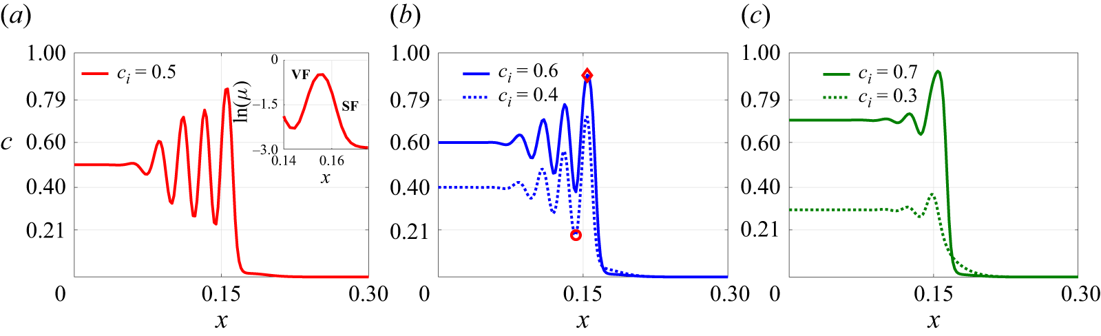


 Open access