


I. Introduction
Given a chosen universe of $ M $
assets, conventional wisdom argues that an unconstrained rational investor should invest in all
$ M $
assets, conventional wisdom argues that an unconstrained rational investor should invest in all $ M $
assets to diversify idiosyncratic risk and improve the efficient frontier. However, this is at odds with the concentrated portfolios typically observed in practice among individual investors (Calvet, Campbell, and Sodini (Reference Calvet, Campbell and Sodini2007), Campbell (Reference Campbell2006), and Goetzmann and Kumar (Reference Goetzmann and Kumar2008)) and institutions (Koijen and Yogo (Reference Koijen and Yogo2019)).Footnote 1 As reviewed by Boyle, Garlappi, Uppal, and Wang (Reference Boyle, Garlappi, Uppal and Wang2012), various papers aim to rationalize the concentrated portfolios of investors or to explain them with behavioral biases. Existing explanations consider, for example, transaction costs, short-sale constraints, prospect theory, overconfidence, cost of information, geographical closeness and familiarity, private incentives, or preferences for higher-order moments.
$ M $
assets to diversify idiosyncratic risk and improve the efficient frontier. However, this is at odds with the concentrated portfolios typically observed in practice among individual investors (Calvet, Campbell, and Sodini (Reference Calvet, Campbell and Sodini2007), Campbell (Reference Campbell2006), and Goetzmann and Kumar (Reference Goetzmann and Kumar2008)) and institutions (Koijen and Yogo (Reference Koijen and Yogo2019)).Footnote 1 As reviewed by Boyle, Garlappi, Uppal, and Wang (Reference Boyle, Garlappi, Uppal and Wang2012), various papers aim to rationalize the concentrated portfolios of investors or to explain them with behavioral biases. Existing explanations consider, for example, transaction costs, short-sale constraints, prospect theory, overconfidence, cost of information, geographical closeness and familiarity, private incentives, or preferences for higher-order moments.
Besides behavioral and financial arguments, another motivation for reducing portfolio size is parameter uncertainty (i.e., the parameters governing the asset return distribution are unknown and must be estimated). In theory, the optimal portfolio can only benefit from increased investment opportunities associated with a higher portfolio size. In practice, however, more parameters and portfolio weights must be estimated, which increases estimation risk and hurts out-of-sample performance (Barroso and Saxena (Reference Barroso and Saxena2021), DeMiguel, Garlappi, and Uppal (Reference DeMiguel, Garlappi and Uppal2009b)).
Sparse portfolio selection aims at alleviating parameter uncertainty precisely by reducing the portfolio size. This is typically achieved by imposing lasso-type constraints, also known as soft-thresholding (Ao, Li, and Zheng (Reference Ao, Li and Zheng2019), DeMiguel, Garlappi, Nogales, and Uppal (Reference DeMiguel, Garlappi, Nogales and Uppal2009a), Fan, Zhang, and Yu (Reference Fan, Zhang and Yu2012), and Yen (Reference Yen2016)) or cardinality constraints (Du, Guo, and Wang (Reference Du, Guo and Wang2023), Gao and Li (Reference Gao and Li2013)). However, these methods suffer from five main drawbacks. First, the optimization programs must be solved in dimension $ M $
and therefore face large estimation risk, even if the output portfolio is ultimately of lower dimension. Second, they can be computationally intensive in high dimension. For instance, cardinality constraints render the portfolio problem NP-hard. Third, they entangle the selection of the assets with the optimization of portfolio weights in one single step. Therefore, sparse methods do not allow for different rebalancing frequencies for portfolio weights and the asset selection, or for flexibility in the asset selection. Fourth, they generally feature hyperparameters that are often estimated by cross-validation, which is time-consuming and adds an extra layer of estimation risk. Lastly, the resulting portfolio size
$ M $
and therefore face large estimation risk, even if the output portfolio is ultimately of lower dimension. Second, they can be computationally intensive in high dimension. For instance, cardinality constraints render the portfolio problem NP-hard. Third, they entangle the selection of the assets with the optimization of portfolio weights in one single step. Therefore, sparse methods do not allow for different rebalancing frequencies for portfolio weights and the asset selection, or for flexibility in the asset selection. Fourth, they generally feature hyperparameters that are often estimated by cross-validation, which is time-consuming and adds an extra layer of estimation risk. Lastly, the resulting portfolio size $ N $
is implicit from the portfolio weights and does not have a clear meaning.
$ N $
is implicit from the portfolio weights and does not have a clear meaning.
To address these drawbacks of sparse portfolio selection, we propose a sequential three-stage process. First, select a portfolio strategy. In this article, we consider a class of portfolio strategies that consists of different combinations of sample mean–variance (MV), global-minimum-variance (GMV), and equal-weighted (EW) portfolios. Although more sophisticated strategies exist, this class has the benefit of being simple, theoretically important, commonly considered in the literature, and allows analytical tractability in finite samples. Second, compute an optimal portfolio size $ N\le M $
. Third, select which
$ N\le M $
. Third, select which $ N $
assets to invest in among the
$ N $
assets to invest in among the $ M $
available ones and optimize the weights on the
$ M $
available ones and optimize the weights on the $ N $
assets with the strategy in step one. Interestingly, Ao et al. (Reference Ao, Li and Zheng2019) propose a similar sequential process for reasons of computational efficiency, selecting a chosen number of
$ N $
assets with the strategy in step one. Interestingly, Ao et al. (Reference Ao, Li and Zheng2019) propose a similar sequential process for reasons of computational efficiency, selecting a chosen number of $ N $
assets to maximize the Sharpe ratio and then implementing their MAXSER strategy on this subset. Specifically, among the S&P 500 stocks, they arbitrarily select 50 of them. In contrast, we show how to select an optimal
$ N $
assets to maximize the Sharpe ratio and then implementing their MAXSER strategy on this subset. Specifically, among the S&P 500 stocks, they arbitrarily select 50 of them. In contrast, we show how to select an optimal $ N $
for several portfolio rules based on estimation-risk considerations.
$ N $
for several portfolio rules based on estimation-risk considerations.
Two key questions remain in our three-stage process: How do we find the optimal portfolio size $ N $
? And how do we then select the
$ N $
? And how do we then select the $ N $
assets? We focus on the first question. Specifically, we introduce a methodology for finding the optimal
$ N $
assets? We focus on the first question. Specifically, we introduce a methodology for finding the optimal $ N $
and leave flexibility to the investor as to the choice of the
$ N $
and leave flexibility to the investor as to the choice of the $ N $
assets. In our empirical analysis, we evaluate the performance of our optimal
$ N $
assets. In our empirical analysis, we evaluate the performance of our optimal $ N $
on 10 simple and sensible asset selection rules as an illustration.
$ N $
on 10 simple and sensible asset selection rules as an illustration.
To find the optimal $ N $
, we consider a classical setting in which investors are expected-utility maximizers with MV preferences, face no investment constraints, and returns are IID multivariate elliptically distributed. In this setting, parameter uncertainty stems from the unknown mean, covariance matrix, and fat tails of returns, which we assume are constant over time. For different portfolio rules within the class of MV portfolio combination strategies we consider, we find the optimal portfolio size
$ N $
, we consider a classical setting in which investors are expected-utility maximizers with MV preferences, face no investment constraints, and returns are IID multivariate elliptically distributed. In this setting, parameter uncertainty stems from the unknown mean, covariance matrix, and fat tails of returns, which we assume are constant over time. For different portfolio rules within the class of MV portfolio combination strategies we consider, we find the optimal portfolio size $ N $
, using a finite-sample setting that trades off between two opposite goals: increasing investment opportunities and reducing estimation risk. This
$ N $
, using a finite-sample setting that trades off between two opposite goals: increasing investment opportunities and reducing estimation risk. This $ N $
is optimal as it maximizes the expected out-of-sample utility (EU), the standard portfolio performance measure under parameter uncertainty (Kan and Zhou (Reference Kan and Zhou2007), Kan, Wang, and Zhou (Reference Kan, Wang and Zhou2021), and Tu and Zhou (Reference Tu and Zhou2011)), and it varies across portfolio rules depending on their estimation risk. We observe empirically that determining the optimal
$ N $
is optimal as it maximizes the expected out-of-sample utility (EU), the standard portfolio performance measure under parameter uncertainty (Kan and Zhou (Reference Kan and Zhou2007), Kan, Wang, and Zhou (Reference Kan, Wang and Zhou2021), and Tu and Zhou (Reference Tu and Zhou2011)), and it varies across portfolio rules depending on their estimation risk. We observe empirically that determining the optimal $ N $
using our theory and selecting the
$ N $
using our theory and selecting the $ N $
assets using different selection rules significantly outperforms investing in all
$ N $
assets using different selection rules significantly outperforms investing in all $ M $
assets in almost 90% of considered configurations.
$ M $
assets in almost 90% of considered configurations.
Our approach has five main benefits compared with the aforementioned sparse methods. First, because we derive the portfolio size before optimizing the portfolio weights, these weights depend on a more limited number of parameters and, thus, face less estimation risk. Second, our approach is computationally less expensive because our optimal $ N $
can be found very efficiently and the portfolio weights are then optimized on a universe of smaller dimension. Third, our optimal
$ N $
can be found very efficiently and the portfolio weights are then optimized on a universe of smaller dimension. Third, our optimal $ N $
depends on the data, the portfolio strategy, and the objective function, but is agnostic as to the selection rule determining which
$ N $
depends on the data, the portfolio strategy, and the objective function, but is agnostic as to the selection rule determining which $ N $
assets to invest in (i.e., the investor has flexibility regarding asset selection). This allows different rebalancing frequencies for portfolio weights and asset selection, which is valuable in practice.Footnote 2 Fourth, our approach does not require the calibration of any hyperparameter such as a constraint threshold. Lastly, the optimal
$ N $
assets to invest in (i.e., the investor has flexibility regarding asset selection). This allows different rebalancing frequencies for portfolio weights and asset selection, which is valuable in practice.Footnote 2 Fourth, our approach does not require the calibration of any hyperparameter such as a constraint threshold. Lastly, the optimal $ N $
has an intuitive meaning from trading off between investment opportunities and estimation risk when maximizing expected utility.
$ N $
has an intuitive meaning from trading off between investment opportunities and estimation risk when maximizing expected utility.
Our theoretical analysis starts with the sample MV (SMV) portfolio, which is optimal in sample, but not out of sample. Assuming that asset returns are equicorrelated as advocated by Engle and Kelly (Reference Engle and Kelly2012) and Clements, Scott, and Silvennoinen (Reference Clements, Scott and Silvennoinen2015),Footnote 3 we express the EU of this portfolio as a function of the portfolio size, the sample size, the correlation, the assets’ Sharpe ratios, and three parameters that measure the impact of fat tails.Footnote 4 We show that because SMV is highly sensitive to estimation errors, its optimal $ N $
is typically very small. As a remedy for this large estimation risk, Kan and Zhou (Reference Kan and Zhou2007) introduce a two-fund rule (2F) that scales down the SMV portfolio by combining it with the risk-free asset to maximize the EU, which Kan and Lassance (Reference Kan and Lassance2025) extend to the case with IID multivariate elliptical returns. Building on this, we derive the optimal
$ N $
is typically very small. As a remedy for this large estimation risk, Kan and Zhou (Reference Kan and Zhou2007) introduce a two-fund rule (2F) that scales down the SMV portfolio by combining it with the risk-free asset to maximize the EU, which Kan and Lassance (Reference Kan and Lassance2025) extend to the case with IID multivariate elliptical returns. Building on this, we derive the optimal $ N $
for the 2F. Remarkably, for typical levels of rather high correlations in equity data, this optimal
$ N $
for the 2F. Remarkably, for typical levels of rather high correlations in equity data, this optimal $ N $
is slightly below half the sample size. Given commonly used sample sizes (e.g., 120 months), this result means that, under the 2F, a finite-sample setting, and our model assumptions, it is optimal to limit the portfolio size to optimize the out-of-sample performance.
$ N $
is slightly below half the sample size. Given commonly used sample sizes (e.g., 120 months), this result means that, under the 2F, a finite-sample setting, and our model assumptions, it is optimal to limit the portfolio size to optimize the out-of-sample performance.
In addition to the 2F, we derive the optimal $ N $
for three-fund rules combining the SMV portfolio, the sample GMV (SGMV) portfolio, and the risk-free asset as in Kan and Zhou (Reference Kan and Zhou2007), DeMiguel, Martín-Utrera, and Nogales (Reference DeMiguel, Martín-Utrera and Nogales2015), and Yuan and Zhou (Reference Yuan and Zhou2024), or combining the SMV portfolio, the EW portfolio, and the risk-free asset as in Tu and Zhou (Reference Tu and Zhou2011), Kan and Wang (Reference Kan and Wang2023), and Lassance, Vanderveken, and Vrins (Reference Lassance, Vanderveken and Vrins2024). Similar to the 2F, the optimal
$ N $
for three-fund rules combining the SMV portfolio, the sample GMV (SGMV) portfolio, and the risk-free asset as in Kan and Zhou (Reference Kan and Zhou2007), DeMiguel, Martín-Utrera, and Nogales (Reference DeMiguel, Martín-Utrera and Nogales2015), and Yuan and Zhou (Reference Yuan and Zhou2024), or combining the SMV portfolio, the EW portfolio, and the risk-free asset as in Tu and Zhou (Reference Tu and Zhou2011), Kan and Wang (Reference Kan and Wang2023), and Lassance, Vanderveken, and Vrins (Reference Lassance, Vanderveken and Vrins2024). Similar to the 2F, the optimal $ N $
for these rules is slightly below half the sample size for typical equity–return correlations. These results extend the literature on portfolio choice with estimation risk by showing that it is beneficial to substantially reduce the portfolio size even after optimally combining the SMV portfolio with robust strategies.
$ N $
for these rules is slightly below half the sample size for typical equity–return correlations. These results extend the literature on portfolio choice with estimation risk by showing that it is beneficial to substantially reduce the portfolio size even after optimally combining the SMV portfolio with robust strategies.
We test our theory first in simulations where we assess the performance of our optimal $ N $
when i) it is subject to estimation errors, ii) asset returns are not equicorrelated, and iii) the selection of the
$ N $
when i) it is subject to estimation errors, ii) asset returns are not equicorrelated, and iii) the selection of the $ N $
assets out of the
$ N $
assets out of the $ M $
available ones is random. The main conclusion is that the size-optimized two-fund and three-fund rules still deliver an EU close to the maximum and substantially larger than that when investing in all
$ M $
available ones is random. The main conclusion is that the size-optimized two-fund and three-fund rules still deliver an EU close to the maximum and substantially larger than that when investing in all $ M $
assets or in too few assets. This shows that our method delivers a satisfying performance even when relaxing the theoretical assumptions, highlighting its practical relevance. Moreover, the simulation analysis allows us to illustrate that, for realistic values of the sample size, our size-optimized two-fund and three-fund rules can outperform more sophisticated benchmark MV portfolios that reduce the portfolio size using soft or hard-thresholding, as well as a factor-plus-alpha (F+A) strategy built on PCA (principal component analysis) and the arbitrage portfolio of Da, Nagel, and Xiu (Reference Da, Nagel and Xiu2024).
$ M $
assets or in too few assets. This shows that our method delivers a satisfying performance even when relaxing the theoretical assumptions, highlighting its practical relevance. Moreover, the simulation analysis allows us to illustrate that, for realistic values of the sample size, our size-optimized two-fund and three-fund rules can outperform more sophisticated benchmark MV portfolios that reduce the portfolio size using soft or hard-thresholding, as well as a factor-plus-alpha (F+A) strategy built on PCA (principal component analysis) and the arbitrage portfolio of Da, Nagel, and Xiu (Reference Da, Nagel and Xiu2024).
Finally, we turn to empirical data. We consider six data sets of characteristic and industry-sorted portfolios and one data set of individual stocks, with $ M $
around 100. Using a rolling window of 120 months, we compare the net out-of-sample utility of 11 portfolio strategies, including our size-optimized two-fund and three-fund rules. For the latter, we propose 10 simple and sensible selection rules to decide which
$ M $
around 100. Using a rolling window of 120 months, we compare the net out-of-sample utility of 11 portfolio strategies, including our size-optimized two-fund and three-fund rules. For the latter, we propose 10 simple and sensible selection rules to decide which $ N $
assets to select. We find large benefits from optimizing
$ N $
assets to select. We find large benefits from optimizing $ N $
using our theory. In the vast majority of cases, the two-fund and three-fund rules implemented with the 10 asset selection rules outperform the same rules applied to all
$ N $
using our theory. In the vast majority of cases, the two-fund and three-fund rules implemented with the 10 asset selection rules outperform the same rules applied to all $ M $
assets. The improvement is particularly large and statistically significant when we shrink the covariance matrix. Moreover, for some asset selection rules, our size-optimized portfolio rules consistently outperform the EW and SGMV portfolios, a notoriously difficult task when the data-set dimension
$ M $
assets. The improvement is particularly large and statistically significant when we shrink the covariance matrix. Moreover, for some asset selection rules, our size-optimized portfolio rules consistently outperform the EW and SGMV portfolios, a notoriously difficult task when the data-set dimension $ M $
is comparable with the sample size, as well as soft and hard-thresholding MV portfolios and the F+A strategy.
$ M $
is comparable with the sample size, as well as soft and hard-thresholding MV portfolios and the F+A strategy.
Our article complements existing work that studies the effect of the portfolio size $ N $
using asymptotic theories. In particular, Ao et al. (Reference Ao, Li and Zheng2019) and Da et al. (Reference Da, Nagel and Xiu2024) consider a class of more sophisticated portfolio strategies that treats estimation risk differently from ours via soft-thresholding and a factor model, respectively. They find, under specific assumptions, that they can asymptotically achieve the performance of the population optimal portfolio as both the portfolio size and the sample size go to infinity. That is, in their asymptotic theories, it is optimal to increase
$ N $
using asymptotic theories. In particular, Ao et al. (Reference Ao, Li and Zheng2019) and Da et al. (Reference Da, Nagel and Xiu2024) consider a class of more sophisticated portfolio strategies that treats estimation risk differently from ours via soft-thresholding and a factor model, respectively. They find, under specific assumptions, that they can asymptotically achieve the performance of the population optimal portfolio as both the portfolio size and the sample size go to infinity. That is, in their asymptotic theories, it is optimal to increase $ N $
. We complement these results by studying a simpler, but nonetheless important, class of portfolio strategies for which we can study the out-of-sample performance analytically in a finite-sample setting. In that case, we find that it is optimal to reduce the portfolio size
$ N $
. We complement these results by studying a simpler, but nonetheless important, class of portfolio strategies for which we can study the out-of-sample performance analytically in a finite-sample setting. In that case, we find that it is optimal to reduce the portfolio size $ N $
. Our simulation and empirical results signal that asymptotic theories like those of Ao et al. (Reference Ao, Li and Zheng2019) and Da et al. (Reference Da, Nagel and Xiu2024), which suggest that increasing
$ N $
. Our simulation and empirical results signal that asymptotic theories like those of Ao et al. (Reference Ao, Li and Zheng2019) and Da et al. (Reference Da, Nagel and Xiu2024), which suggest that increasing $ N $
is beneficial, might not kick in for realistic sample sizes and typically deliver a performance inferior to that of our size-optimized portfolios.
$ N $
is beneficial, might not kick in for realistic sample sizes and typically deliver a performance inferior to that of our size-optimized portfolios.
This article is structured as follows: In Section II, we study the optimal portfolio size for the MV portfolio with no parameter uncertainty. In Section III, we show how to derive an optimal $ N $
for the SMV portfolio and the 2F under parameter uncertainty. Sections IV and V contain our simulation and empirical analysis, respectively. Section VI concludes. The Appendix contains results and proofs that are central to the main text. The Supplementary Material provides additional theoretical, simulation, and empirical results.
$ N $
for the SMV portfolio and the 2F under parameter uncertainty. Sections IV and V contain our simulation and empirical analysis, respectively. Section VI concludes. The Appendix contains results and proofs that are central to the main text. The Supplementary Material provides additional theoretical, simulation, and empirical results.
II. Optimal Portfolio Size Without Parameter Uncertainty
In this section, we study the optimal portfolio size for an unconstrained MV investor who knows the parameters of asset returns without uncertainty. We suppose that the investor starts from a universe of $ M $
assets and wishes to find an optimal number
$ M $
assets and wishes to find an optimal number $ N\le M $
of assets.
$ N\le M $
of assets.
Given a fixed number $ N $
of assets, let
$ N $
of assets, let $ {\boldsymbol{r}}_t $
be the
$ {\boldsymbol{r}}_t $
be the $ N\times 1 $
vector of asset excess returns at time
$ N\times 1 $
vector of asset excess returns at time $ t $
, which has a mean
$ t $
, which has a mean $ {\boldsymbol{\mu}}_N $
and a positive-definite covariance matrix
$ {\boldsymbol{\mu}}_N $
and a positive-definite covariance matrix $ {\boldsymbol{\Sigma}}_N $
. We denote by
$ {\boldsymbol{\Sigma}}_N $
. We denote by $ {\mu}_i $
,
$ {\mu}_i $
, $ {\sigma}_i^2 $
, and
$ {\sigma}_i^2 $
, and $ {s}_i={\mu}_i/{\sigma}_i $
the mean excess return, variance, and Sharpe ratio of asset
$ {s}_i={\mu}_i/{\sigma}_i $
the mean excess return, variance, and Sharpe ratio of asset $ i $
. An MV investor with risk-aversion coefficient
$ i $
. An MV investor with risk-aversion coefficient $ \gamma >0 $
selects the portfolio weights on the risky assets as
$ \gamma >0 $
selects the portfolio weights on the risky assets as
 $$ {\boldsymbol{w}}^{\star }=\underset{\boldsymbol{w}\in {\mathrm{\mathbb{R}}}^N}{\arg \max }U\left(\boldsymbol{w}\right)=\underset{\boldsymbol{w}\in {\mathrm{\mathbb{R}}}^N}{\arg \max }{\boldsymbol{w}}^{\prime }{\boldsymbol{\mu}}_N-\frac{\gamma }{2}{\boldsymbol{w}}^{\prime }{\boldsymbol{\Sigma}}_N\boldsymbol{w}, $$
where $ U\left(\boldsymbol{w}\right) $
is the MV utility of portfolio
$ U\left(\boldsymbol{w}\right) $
is the MV utility of portfolio $ \boldsymbol{w} $
. Solving (1) yields the MV portfolio satisfying
$ \boldsymbol{w} $
. Solving (1) yields the MV portfolio satisfying
 $$ {\boldsymbol{w}}^{\star }=\frac{1}{\gamma }{\boldsymbol{\Sigma}}_N^{-1}{\boldsymbol{\mu}}_N\hskip1em \mathrm{and}\hskip1em U\left({\boldsymbol{w}}^{\star}\right)=\frac{\theta_N^2}{2\gamma}\hskip1em \mathrm{with}\hskip1em {\theta}_N^2={\boldsymbol{\mu}}_N^{\prime }{\boldsymbol{\Sigma}}_N^{-1}{\boldsymbol{\mu}}_N, $$
where $ {\theta}_N $
is the maximum Sharpe ratio. We have that
$ {\theta}_N $
is the maximum Sharpe ratio. We have that $ {\boldsymbol{w}}^{\star } $
combines two funds: the fully invested tangency portfolio,
$ {\boldsymbol{w}}^{\star } $
combines two funds: the fully invested tangency portfolio, $ \boldsymbol{w}={\left({\mathbf{1}}_N^{\prime }{\boldsymbol{\Sigma}}_N^{-1}{\boldsymbol{\mu}}_N\right)}^{-1}{\boldsymbol{\Sigma}}_N^{-1}{\boldsymbol{\mu}}_N $
, and the risk-free asset,
$ \boldsymbol{w}={\left({\mathbf{1}}_N^{\prime }{\boldsymbol{\Sigma}}_N^{-1}{\boldsymbol{\mu}}_N\right)}^{-1}{\boldsymbol{\Sigma}}_N^{-1}{\boldsymbol{\mu}}_N $
, and the risk-free asset, $ \boldsymbol{w}={\mathbf{0}}_N $
.
$ \boldsymbol{w}={\mathbf{0}}_N $
.
Clearly, $ U\left({\boldsymbol{w}}^{\star}\right) $
is nondecreasing with
$ U\left({\boldsymbol{w}}^{\star}\right) $
is nondecreasing with $ N $
because one can set the weight of an additional asset to 0 and keep the same utility. Thus, without parameter uncertainty, it is optimal to consider the whole investment universe and set
$ N $
because one can set the weight of an additional asset to 0 and keep the same utility. Thus, without parameter uncertainty, it is optimal to consider the whole investment universe and set $ N=M $
. To relate
$ N=M $
. To relate $ U\left({\boldsymbol{w}}^{\star}\right) $
and
$ U\left({\boldsymbol{w}}^{\star}\right) $
and $ N $
explicitly, we assume the following about
$ N $
explicitly, we assume the following about $ {\boldsymbol{\Sigma}}_M $
:
$ {\boldsymbol{\Sigma}}_M $
:
Assumption 1. The covariance matrix $ {\boldsymbol{\Sigma}}_M $
takes the form
$ {\boldsymbol{\Sigma}}_M $
takes the form $ {\boldsymbol{\Sigma}}_M\left(\rho \right)={\boldsymbol{D}}_M{\boldsymbol{P}}_M\left(\rho \right){\boldsymbol{D}}_M $
with
$ {\boldsymbol{\Sigma}}_M\left(\rho \right)={\boldsymbol{D}}_M{\boldsymbol{P}}_M\left(\rho \right){\boldsymbol{D}}_M $
with $ {\boldsymbol{D}}_M $
the diagonal matrix of standard deviations and
$ {\boldsymbol{D}}_M $
the diagonal matrix of standard deviations and $ {\boldsymbol{P}}_M\left(\rho \right) $
the equicorrelation matrix,
$ {\boldsymbol{P}}_M\left(\rho \right) $
the equicorrelation matrix,
 $$ {\boldsymbol{P}}_M\left(\rho \right)=\left(1-\rho \right){\boldsymbol{I}}_M+\rho {\mathbf{1}}_M{\mathbf{1}}_M^{\prime }, $$
where $ {\mathbf{1}}_M $
and
$ {\mathbf{1}}_M $
and $ {\boldsymbol{I}}_M $
are the unit vector and matrix, and
$ {\boldsymbol{I}}_M $
are the unit vector and matrix, and $ \rho \in \left(-\frac{1}{M-1},1\right) $
so that
$ \rho \in \left(-\frac{1}{M-1},1\right) $
so that $ {\boldsymbol{\Sigma}}_M $
is invertible.
$ {\boldsymbol{\Sigma}}_M $
is invertible.
Under Assumption 1, the dependence structure depends on a single parameter, $ \rho $
. It follows that for any
$ \rho $
. It follows that for any $ N\le M $
,
$ N\le M $
, $ {\boldsymbol{\Sigma}}_N $
has the same form as in Assumption 1. This assumption is commonly used in portfolio selection to trade off between specification and estimation error.Footnote 5 We use Assumption 1 only as a way to express the EU of our portfolio rules as an explicit function of
$ {\boldsymbol{\Sigma}}_N $
has the same form as in Assumption 1. This assumption is commonly used in portfolio selection to trade off between specification and estimation error.Footnote 5 We use Assumption 1 only as a way to express the EU of our portfolio rules as an explicit function of $ N $
, which will allow us to find the optimal
$ N $
, which will allow us to find the optimal $ N $
. We do not need this assumption for the portfolio weights. In Section OA.1 of the Supplementary Material, we find the optimal
$ N $
. We do not need this assumption for the portfolio weights. In Section OA.1 of the Supplementary Material, we find the optimal $ N $
under another commonly used approximation, the single-factor model, which we show is essentially equivalent to that under equicorrelation.
$ N $
under another commonly used approximation, the single-factor model, which we show is essentially equivalent to that under equicorrelation.
In the next proposition, we provide the analytical expression of $ U\left({\boldsymbol{w}}^{\star}\right) $
under Assumption 1.Footnote 6 This is a novel result to the best of our knowledge.
$ U\left({\boldsymbol{w}}^{\star}\right) $
under Assumption 1.Footnote 6 This is a novel result to the best of our knowledge.
Proposition 1. Under Assumption 1, the utility of the MV portfolio is $ U\left({\boldsymbol{w}}^{\star}\right)={\theta}_N^2/\left(2\gamma \right) $
with
$ U\left({\boldsymbol{w}}^{\star}\right)={\theta}_N^2/\left(2\gamma \right) $
with
 $$ {\theta}_N^2=\frac{N}{1-\rho }{\delta}_N\left({\overline{\boldsymbol{\theta}}}_N\right),\hskip1em {\delta}_N\left({\overline{\boldsymbol{\theta}}}_N\right)={\overline{\theta}}_{N,2}-\frac{N\rho}{1-\rho + N\rho}{\overline{\theta}}_{N,1}^2\ge 0, $$
where $ {\overline{\boldsymbol{\theta}}}_N=\left({\overline{\theta}}_{N,1},{\overline{\theta}}_{N,2}\right) $
and
$ {\overline{\boldsymbol{\theta}}}_N=\left({\overline{\theta}}_{N,1},{\overline{\theta}}_{N,2}\right) $
and $ {\overline{\theta}}_{N,k}=\frac{1}{N}{\sum}_{i=1}^N{s}_i^k $
. Moreover,
$ {\overline{\theta}}_{N,k}=\frac{1}{N}{\sum}_{i=1}^N{s}_i^k $
. Moreover, $ U\left({\boldsymbol{w}}^{\star}\right) $
is nondecreasing in
$ U\left({\boldsymbol{w}}^{\star}\right) $
is nondecreasing in $ N $
and is strictly increasing from
$ N $
and is strictly increasing from $ N $
to
$ N $
to $ N+1 $
whenever
$ N+1 $
whenever $ {s}_{N+1}\ne \rho N{\overline{\theta}}_{N,1}/\left(1-\rho + N\rho \right) $
.
$ {s}_{N+1}\ne \rho N{\overline{\theta}}_{N,1}/\left(1-\rho + N\rho \right) $
.
Proposition 1 shows that the maximum utility is nondecreasing in $ N $
. In Figure 1, we depict
$ N $
. In Figure 1, we depict $ U\left({\boldsymbol{w}}^{\star}\right) $
as a function of
$ U\left({\boldsymbol{w}}^{\star}\right) $
as a function of $ N\in \left\{1,\dots, M\right\} $
for
$ N\in \left\{1,\dots, M\right\} $
for $ \rho \in \left\{\mathrm{0.2,0.5,0.8}\right\} $
and assets’ monthly Sharpe ratios
$ \rho \in \left\{\mathrm{0.2,0.5,0.8}\right\} $
and assets’ monthly Sharpe ratios $ {s}_i $
calibrated to a data set of
$ {s}_i $
calibrated to a data set of $ M=96 $
decile portfoliosFootnote 7 sorted on size and book-to-market (96S-BM) spanning July 1963 to August 2023.Footnote 8
$ M=96 $
decile portfoliosFootnote 7 sorted on size and book-to-market (96S-BM) spanning July 1963 to August 2023.Footnote 8
Figure 1 depicts $ U\left({\boldsymbol{w}}^{\star}\right) $
in equation (4) as a function of the portfolio size
$ U\left({\boldsymbol{w}}^{\star}\right) $
in equation (4) as a function of the portfolio size $ N $
under the assumption that asset returns are equicorrelated with a correlation
$ N $
under the assumption that asset returns are equicorrelated with a correlation $ \rho \in \left\{\mathrm{0.2,0.5,0.8}\right\} $
. We calibrate the assets’ monthly Sharpe ratios to a data set of
$ \rho \in \left\{\mathrm{0.2,0.5,0.8}\right\} $
. We calibrate the assets’ monthly Sharpe ratios to a data set of $ M=96 $
portfolios sorted on size and book-to-market spanning July 1963 to August 2023. Starting with
$ M=96 $
portfolios sorted on size and book-to-market spanning July 1963 to August 2023. Starting with $ N=1 $
asset chosen randomly, we compute
$ N=1 $
asset chosen randomly, we compute $ U\left({\boldsymbol{w}}^{\star}\right) $
. Then, we add a randomly selected asset not previously selected and compute
$ U\left({\boldsymbol{w}}^{\star}\right) $
. Then, we add a randomly selected asset not previously selected and compute $ U\left({\boldsymbol{w}}^{\star}\right) $
again. We continue this procedure until
$ U\left({\boldsymbol{w}}^{\star}\right) $
again. We continue this procedure until $ N=M $
. We repeat this procedure
$ N=M $
. We repeat this procedure $ \mathrm{10,000} $
times and depict the average
$ \mathrm{10,000} $
times and depict the average $ U\left({\boldsymbol{w}}^{\star}\right) $
over all draws. We consider a risk-aversion coefficient
$ U\left({\boldsymbol{w}}^{\star}\right) $
over all draws. We consider a risk-aversion coefficient $ \gamma =1 $
.
$ \gamma =1 $
.

III. Optimal Portfolio Size Under Parameter Uncertainty
In this section, we show that it is no longer optimal for an MV investor to invest in all $ M $
assets when the assets’ parameters are unknown and the investor relies on sample estimates.
$ M $
assets when the assets’ parameters are unknown and the investor relies on sample estimates.
A. Sample Estimates and Distributional Assumption
Given a sample of asset excess returns of size $ T $
,
$ T $
, $ \left({\boldsymbol{r}}_1,\dots, {\boldsymbol{r}}_T\right) $
, let
$ \left({\boldsymbol{r}}_1,\dots, {\boldsymbol{r}}_T\right) $
, let
 $$ {\hat{\boldsymbol{\mu}}}_N=\frac{1}{T}\sum \limits_{t=1}^T{\boldsymbol{r}}_t\hskip1em \mathrm{and}\hskip1em {\hat{\boldsymbol{\Sigma}}}_N=\frac{1}{T}\sum \limits_{t=1}^T\left({\boldsymbol{r}}_t-{\hat{\boldsymbol{\mu}}}_N\right){\left({\boldsymbol{r}}_t-{\hat{\boldsymbol{\mu}}}_N\right)}^{\prime } $$
be the sample estimates of $ {\boldsymbol{\mu}}_N $
and
$ {\boldsymbol{\mu}}_N $
and $ {\boldsymbol{\Sigma}}_N $
, and we require
$ {\boldsymbol{\Sigma}}_N $
, and we require $ T>N $
so that
$ T>N $
so that $ {\hat{\boldsymbol{\Sigma}}}_N $
is almost surely invertible. Given a sample portfolio
$ {\hat{\boldsymbol{\Sigma}}}_N $
is almost surely invertible. Given a sample portfolio $ \hat{\boldsymbol{w}} $
estimated with
$ \hat{\boldsymbol{w}} $
estimated with $ {\hat{\boldsymbol{\mu}}}_N $
and
$ {\hat{\boldsymbol{\mu}}}_N $
and $ {\hat{\boldsymbol{\Sigma}}}_N $
, we measure its performance with the EU pioneered by Kan and Zhou (Reference Kan and Zhou2007),
$ {\hat{\boldsymbol{\Sigma}}}_N $
, we measure its performance with the EU pioneered by Kan and Zhou (Reference Kan and Zhou2007),
 $$ EU\left(\hat{\boldsymbol{w}}\right)=\unicode{x1D53C}\left[U\left(\hat{\boldsymbol{w}}\right)\right]=\unicode{x1D53C}\left[{\hat{\boldsymbol{w}}}^{\prime }{\boldsymbol{\mu}}_N-\frac{\gamma }{2}{\hat{\boldsymbol{w}}}^{\prime }{\boldsymbol{\Sigma}}_N\hat{\boldsymbol{w}}\right]. $$
We then define $ {N}^{\star } $
as the optimal portfolio size
$ {N}^{\star } $
as the optimal portfolio size $ N $
maximizing the EU of
$ N $
maximizing the EU of $ \hat{\boldsymbol{w}} $
.
$ \hat{\boldsymbol{w}} $
.
Kan and Zhou (Reference Kan and Zhou2007) and follow-up papers, such as Tu and Zhou (Reference Tu and Zhou2011), Kan et al. (Reference Kan, Wang and Zhou2021), Lassance et al. (Reference Lassance, Vanderveken and Vrins2024), Lassance, Martín-Utrera, and Simaan (Reference Lassance, Martín-Utrera and Simaan2024), and Yuan and Zhou (Reference Yuan and Zhou2024), evaluate (6) under the IID multivariate normal distributional assumption. Instead, we follow Kan and Lassance (Reference Kan and Lassance2025), who study the EU of various sample portfolios under the IID multivariate elliptical distribution. Like them, we use the stochastic representation of the elliptical distribution in El Karoui (Reference El Karoui2010), (Reference El Karoui2013).
Assumption 2. Asset returns $ {\boldsymbol{r}}_t $
are IID over time and follow a multivariate elliptical distribution. That is,
$ {\boldsymbol{r}}_t $
are IID over time and follow a multivariate elliptical distribution. That is, $ {\boldsymbol{r}}_{t_1}\perp {\boldsymbol{r}}_{t_2} $
for
$ {\boldsymbol{r}}_{t_1}\perp {\boldsymbol{r}}_{t_2} $
for $ {t}_1\ne {t}_2 $
and
$ {t}_1\ne {t}_2 $
and $ {\boldsymbol{r}}_t\overset{d}{=}{\boldsymbol{\mu}}_M+{\left(\tau {\boldsymbol{\Sigma}}_M\right)}^{\frac{1}{2}}{\mathbf{z}}_M $
, where
$ {\boldsymbol{r}}_t\overset{d}{=}{\boldsymbol{\mu}}_M+{\left(\tau {\boldsymbol{\Sigma}}_M\right)}^{\frac{1}{2}}{\mathbf{z}}_M $
, where $ {\mathbf{z}}_M\sim \mathcal{N}\left({\mathbf{0}}_M,{\boldsymbol{I}}_M\right) $
,
$ {\mathbf{z}}_M\sim \mathcal{N}\left({\mathbf{0}}_M,{\boldsymbol{I}}_M\right) $
, $ \tau $
is a positive random variable satisfying
$ \tau $
is a positive random variable satisfying $ \unicode{x1D53C}\left[\tau \right]=1 $
, and
$ \unicode{x1D53C}\left[\tau \right]=1 $
, and $ {\mathbf{z}}_M\perp \tau $
. In particular,
$ {\mathbf{z}}_M\perp \tau $
. In particular, $ {\boldsymbol{\mu}}_M $
and
$ {\boldsymbol{\mu}}_M $
and $ {\boldsymbol{\Sigma}}_M $
are constant over time.
$ {\boldsymbol{\Sigma}}_M $
are constant over time.
We recover the normal distribution when $ \tau =1 $
and the
$ \tau =1 $
and the $ t $
-distribution when
$ t $
-distribution when $ \tau \sim \left(\nu -2\right)/{\chi}_{\nu}^2 $
, where
$ \tau \sim \left(\nu -2\right)/{\chi}_{\nu}^2 $
, where $ {\chi}_{\nu}^2 $
is a chi-square distribution with
$ {\chi}_{\nu}^2 $
is a chi-square distribution with $ \nu >2 $
degrees of freedom. We focus on the elliptical distribution because it is consistent with MV portfolios (Chamberlain (Reference Chamberlain1983), Schuhmacher, Kohrs, and Auer (Reference Schuhmacher, Kohrs and Auer2021)). Specifically, since the multivariate elliptical distribution is closed under linear transformations, all portfolios have the same higher moments and only differ in their mean return and variance. Therefore, for all increasing and concave utility functions, the optimal portfolio under expected utility is MV efficient. We also opt for the elliptical distribution because Kan and Lassance (Reference Kan and Lassance2025) show that accounting for fat tails is crucial in determining optimal portfolio combination rules.
$ \nu >2 $
degrees of freedom. We focus on the elliptical distribution because it is consistent with MV portfolios (Chamberlain (Reference Chamberlain1983), Schuhmacher, Kohrs, and Auer (Reference Schuhmacher, Kohrs and Auer2021)). Specifically, since the multivariate elliptical distribution is closed under linear transformations, all portfolios have the same higher moments and only differ in their mean return and variance. Therefore, for all increasing and concave utility functions, the optimal portfolio under expected utility is MV efficient. We also opt for the elliptical distribution because Kan and Lassance (Reference Kan and Lassance2025) show that accounting for fat tails is crucial in determining optimal portfolio combination rules.
B. Optimal Portfolio Size for Sample Portfolios
The first strategy we consider is the sample counterpart of the MV portfolio in (2), that is,
 $$ {\hat{\boldsymbol{w}}}^{\star }=\frac{1}{\gamma }{\hat{\boldsymbol{\Sigma}}}_N^{-1}{\hat{\boldsymbol{\mu}}}_N. $$
The SMV portfolio is not robust to parameter uncertainty because it is only optimal in sample. Therefore, we also consider the 2F of Kan and Zhou (Reference Kan and Zhou2007) that scales down the SMV portfolio to maximize its EU. This 2F is of the form
 $$ \hat{\boldsymbol{w}}\left(\alpha \right)=\alpha {\hat{\boldsymbol{w}}}^{\star }=\frac{\alpha }{\gamma }{\hat{\boldsymbol{\Sigma}}}_N^{-1}{\hat{\boldsymbol{\mu}}}_N, $$
where $ \alpha \in \mathrm{\mathbb{R}} $
is the combination coefficient. The SMV in (7) corresponds to
$ \alpha \in \mathrm{\mathbb{R}} $
is the combination coefficient. The SMV in (7) corresponds to $ {\hat{\boldsymbol{w}}}^{\star }=\overset{}{\hat{\boldsymbol{w}}}(\alpha =1) $
.
$ {\hat{\boldsymbol{w}}}^{\star }=\overset{}{\hat{\boldsymbol{w}}}(\alpha =1) $
.
In the next proposition, we derive the EU of the 2F and, thus, also the SMV portfolio, the optimal combination coefficient $ {\alpha}^{\star } $
, and which EU it delivers, when asset returns are elliptically distributed. These results then allow us to determine the optimal portfolio size
$ {\alpha}^{\star } $
, and which EU it delivers, when asset returns are elliptically distributed. These results then allow us to determine the optimal portfolio size $ N $
. This proposition follows, with minor adjustments, from Kan and Lassance ((Reference Kan and Lassance2025), Propositions 7 and 8). In Appendix A.I, we follow the same approach for three-fund rules that extend the 2F by incorporating a third fully invested fund that is either the GMV or the EW portfolio. We refer to these as the GMV-three-fund rule (3FGMV) and the EW-three-fund rule (3FEW), respectively.
$ N $
. This proposition follows, with minor adjustments, from Kan and Lassance ((Reference Kan and Lassance2025), Propositions 7 and 8). In Appendix A.I, we follow the same approach for three-fund rules that extend the 2F by incorporating a third fully invested fund that is either the GMV or the EW portfolio. We refer to these as the GMV-three-fund rule (3FGMV) and the EW-three-fund rule (3FEW), respectively.
Proposition 2. Let $ T>N+4 $
,
$ T>N+4 $
, $ \boldsymbol{M}={\boldsymbol{I}}_T-{\mathbf{1}}_T{\mathbf{1}}_T^{\prime }/T $
,
$ \boldsymbol{M}={\boldsymbol{I}}_T-{\mathbf{1}}_T{\mathbf{1}}_T^{\prime }/T $
, $ {\boldsymbol{Z}}_N $
be a
$ {\boldsymbol{Z}}_N $
be a $ T\times N $
matrix of independent standard normal variables,
$ T\times N $
matrix of independent standard normal variables, $ \boldsymbol{\Lambda} $
be a diagonal matrix of
$ \boldsymbol{\Lambda} $
be a diagonal matrix of $ T $
independent copies of
$ T $
independent copies of $ {\tau}^{1/2} $
, and
$ {\tau}^{1/2} $
, and $ \boldsymbol{\Lambda} \perp {\boldsymbol{Z}}_N $
. Then, under Assumption 2, the EU of the 2F
$ \boldsymbol{\Lambda} \perp {\boldsymbol{Z}}_N $
. Then, under Assumption 2, the EU of the 2F $ \hat{\boldsymbol{w}}\left(\alpha \right) $
in (8) is
$ \hat{\boldsymbol{w}}\left(\alpha \right) $
in (8) is
 $$ EU\left(\hat{\boldsymbol{w}}\left(\alpha \right)\right)=\frac{T}{2\gamma \left(T-N-2\right)}\left[\left(2{\alpha \kappa}_{N,1}-\frac{c_N{\alpha}^2{\kappa}_{N,2}T}{T-N-2}\right){\theta}_N^2-\frac{c_N{\alpha}^2{\kappa}_{N,3}N}{T-N-2}\right], $$
where $ {\theta}_N^2 $
is the maximum squared Sharpe ratio given in (4),
$ {\theta}_N^2 $
is the maximum squared Sharpe ratio given in (4), $ {c}_N=\frac{\left(T-2\right)\left(T-N-2\right)}{\left(T-N-1\right)\left(T-N-4\right)} $
, and
$ {c}_N=\frac{\left(T-2\right)\left(T-N-2\right)}{\left(T-N-1\right)\left(T-N-4\right)} $
, and $ {\kappa}_{N,1} $
,
$ {\kappa}_{N,1} $
, $ {\kappa}_{N,2} $
, and
$ {\kappa}_{N,2} $
, and $ {\kappa}_{N,3} $
, which we assume exist, are the functions of only
$ {\kappa}_{N,3} $
, which we assume exist, are the functions of only $ N $
,
$ N $
, $ T $
, and the distribution of
$ T $
, and the distribution of $ \tau $
:
$ \tau $
:
 $$ {\kappa}_{N,1}=\frac{T-N-2}{N}\unicode{x1D53C}\left[\mathrm{tr}\left({\left({\boldsymbol{Z}}_N^{\prime}\boldsymbol{\Lambda} \boldsymbol{M}\boldsymbol{\Lambda } {\boldsymbol{Z}}_N\right)}^{-1}\right)\right], $$
 $$ {\kappa}_{N,2}=\frac{{\left(T-N-2\right)}^2}{c_NN}\unicode{x1D53C}\left[\mathrm{tr}\left({\left({\boldsymbol{Z}}_N^{\prime}\boldsymbol{\Lambda} \boldsymbol{M}\boldsymbol{\Lambda } {\boldsymbol{Z}}_N\right)}^{-2}\right)\right], $$
 $$ {\kappa}_{N,3}=\frac{{\left(T-N-2\right)}^2}{c_N NT}\unicode{x1D53C}\left[{\mathbf{1}}_T^{\prime}\boldsymbol{\Lambda} {\boldsymbol{Z}}_N{\left({\boldsymbol{Z}}_N^{\prime}\boldsymbol{\Lambda} \boldsymbol{M}\boldsymbol{\Lambda } {\boldsymbol{Z}}_N\right)}^{-2}{\boldsymbol{Z}}_N^{\prime}\boldsymbol{\Lambda} {\mathbf{1}}_T\right]. $$
Moreover, the optimal combination coefficient $ {\alpha}^{\star } $
maximizing (9) and the resulting EU are
$ {\alpha}^{\star } $
maximizing (9) and the resulting EU are
 $$ {\alpha}^{\star }=\frac{T-N-2}{c_NT}\left(\frac{\kappa_{N,1}{\theta}_N^2}{\kappa_{N,2}{\theta}_N^2+{\kappa}_{N,3}\frac{N}{T}}\right)\hskip0.66em \mathrm{and}\hskip0.66em EU\left(\hat{\boldsymbol{w}}\left({\alpha}^{\star}\right)\right)=\frac{1}{2\gamma {c}_N}\left(\frac{\kappa_{N,1}^2{\theta}_N^4}{\kappa_{N,2}{\theta}_N^2+{\kappa}_{N,3}\frac{N}{T}}\right). $$
Three comments are in order. First, Proposition 2 is valid for any $ {\boldsymbol{\Sigma}}_N $
, not only those of the form
$ {\boldsymbol{\Sigma}}_N $
, not only those of the form $ {\boldsymbol{\Sigma}}_N\left(\rho \right) $
. Second,
$ {\boldsymbol{\Sigma}}_N\left(\rho \right) $
. Second, $ {\kappa}_{N,1} $
,
$ {\kappa}_{N,1} $
, $ {\kappa}_{N,2} $
, and
$ {\kappa}_{N,2} $
, and $ {\kappa}_{N,3} $
do not have a closed-form expression, but can be evaluated via Monte Carlo simulations given the distribution of
$ {\kappa}_{N,3} $
do not have a closed-form expression, but can be evaluated via Monte Carlo simulations given the distribution of $ \tau $
. We explain how we estimate them in Appendix A.II. Kan and Lassance (Reference Kan and Lassance2025) show that they increase with estimation risk
$ \tau $
. We explain how we estimate them in Appendix A.II. Kan and Lassance (Reference Kan and Lassance2025) show that they increase with estimation risk $ N/T $
and tail heaviness. Third, under parameter uncertainty in
$ N/T $
and tail heaviness. Third, under parameter uncertainty in $ {\boldsymbol{\mu}}_N $
and
$ {\boldsymbol{\mu}}_N $
and $ {\boldsymbol{\Sigma}}_N $
, a larger
$ {\boldsymbol{\Sigma}}_N $
, a larger $ N $
may not always be favorable. Instead, the
$ N $
may not always be favorable. Instead, the $ N $
maximizing (9) trades off between improving the population performance (i.e., increasing
$ N $
maximizing (9) trades off between improving the population performance (i.e., increasing $ {\theta}_N^2 $
) and limiting estimation risk (i.e., decreasing
$ {\theta}_N^2 $
) and limiting estimation risk (i.e., decreasing $ N/T $
).
$ N/T $
).
Next, we proceed as in Section II and relate the EU with $ N $
more explicitly by assuming that the covariance matrix
$ N $
more explicitly by assuming that the covariance matrix $ {\boldsymbol{\Sigma}}_N $
complies with Assumption 1 (i.e.,
$ {\boldsymbol{\Sigma}}_N $
complies with Assumption 1 (i.e., $ {\boldsymbol{\Sigma}}_N={\boldsymbol{\Sigma}}_N\left(\rho \right) $
). We obtain this novel result by plugging the expression for
$ {\boldsymbol{\Sigma}}_N={\boldsymbol{\Sigma}}_N\left(\rho \right) $
). We obtain this novel result by plugging the expression for $ {\theta}_N^2 $
under equicorrelation in (4) into equations (9) and (13).
$ {\theta}_N^2 $
under equicorrelation in (4) into equations (9) and (13).
Corollary 1. Under Assumptions 1 and 2, the EU of the SMV portfolio $ {\hat{\boldsymbol{w}}}^{\star } $
and the optimal 2F
$ {\hat{\boldsymbol{w}}}^{\star } $
and the optimal 2F $ \hat{\boldsymbol{w}}\left({\alpha}^{\star}\right) $
are given by
$ \hat{\boldsymbol{w}}\left({\alpha}^{\star}\right) $
are given by
 $$ EU\left({\hat{\boldsymbol{w}}}^{\star}\right)=\frac{NT}{2\gamma \left(T-N-2\right)}\left[\frac{\delta_N\left({\overline{\boldsymbol{\theta}}}_N\right)}{1-\rho}\left(2{\kappa}_{N,1}-\frac{c_N{\kappa}_{N,2}T}{T-N-2}\right)-\frac{c_N{\kappa}_{N,3}}{T-N-2}\right] $$
 $$ =: E{U}_{smv}\left(N,T,\rho, \tau, {\bar{\theta}}_N\right),\hskip0.33em \mathrm{and} $$
 $$ EU\left(\hat{\boldsymbol{w}}\left({\alpha}^{\star}\right)\right)=\frac{N}{2\gamma {c}_N\left(1-\rho \right)}\times \frac{\kappa_{N,1}^2{\delta}_N{\left({\overline{\boldsymbol{\theta}}}_N\right)}^2}{\kappa_{N,2}{\delta}_N\left({\overline{\boldsymbol{\theta}}}_N\right)+{\kappa}_{N,3}\frac{1-\rho }{T}}=: {EU}_{2f}\left(N,T,\rho, \tau, {\overline{\boldsymbol{\theta}}}_N\right). $$ $ {EU}_{smv} $
and
$ {EU}_{smv} $
and $ {EU}_{2f} $
depend on several parameters.Footnote 9 First, the sample size
$ {EU}_{2f} $
depend on several parameters.Footnote 9 First, the sample size $ T $
, directly but also via
$ T $
, directly but also via $ {c}_N $
and
$ {c}_N $
and $ \left({\kappa}_{N,1},{\kappa}_{N,2},{\kappa}_{N,3}\right) $
. Second, the portfolio size
$ \left({\kappa}_{N,1},{\kappa}_{N,2},{\kappa}_{N,3}\right) $
. Second, the portfolio size $ N $
, directly but also via
$ N $
, directly but also via $ {c}_N $
, the function
$ {c}_N $
, the function $ {\delta}_N $
, and
$ {\delta}_N $
, and $ \left({\kappa}_{N,1},{\kappa}_{N,2},{\kappa}_{N,3}\right) $
. Third, which
$ \left({\kappa}_{N,1},{\kappa}_{N,2},{\kappa}_{N,3}\right) $
. Third, which $ N $
assets are selected via
$ N $
assets are selected via $ {\overline{\boldsymbol{\theta}}}_N=\left({\overline{\theta}}_{N,1},{\overline{\theta}}_{N,2}\right) $
.
$ {\overline{\boldsymbol{\theta}}}_N=\left({\overline{\theta}}_{N,1},{\overline{\theta}}_{N,2}\right) $
.
Now, to maximize $ {EU}_{smv}\left(N,T,\rho, \tau, {\overline{\boldsymbol{\theta}}}_N\right) $
or
$ {EU}_{smv}\left(N,T,\rho, \tau, {\overline{\boldsymbol{\theta}}}_N\right) $
or $ {EU}_{2f}\left(N,T,\rho, \tau, {\overline{\boldsymbol{\theta}}}_N\right) $
with respect to
$ {EU}_{2f}\left(N,T,\rho, \tau, {\overline{\boldsymbol{\theta}}}_N\right) $
with respect to $ N $
, one would also need to optimize the selection of assets because
$ N $
, one would also need to optimize the selection of assets because $ {\overline{\boldsymbol{\theta}}}_N $
depends on
$ {\overline{\boldsymbol{\theta}}}_N $
depends on $ N $
via the chosen subset of assets. This is a difficult optimization problem because the number of possible subsets of
$ N $
via the chosen subset of assets. This is a difficult optimization problem because the number of possible subsets of $ N $
assets with
$ N $
assets with $ N $
going from 1 to
$ N $
going from 1 to $ M $
grows very quickly with
$ M $
grows very quickly with $ M $
.Footnote 10 Moreover, this would introduce potentially severe estimation risk and time instability in the selection of assets, which is undesirable. This is why, to disentangle the determination of the optimal
$ M $
.Footnote 10 Moreover, this would introduce potentially severe estimation risk and time instability in the selection of assets, which is undesirable. This is why, to disentangle the determination of the optimal $ N $
from the asset selection, we replace
$ N $
from the asset selection, we replace $ {\overline{\boldsymbol{\theta}}}_N $
by its counterpart for the whole investment universe (i.e.,
$ {\overline{\boldsymbol{\theta}}}_N $
by its counterpart for the whole investment universe (i.e., $ {\overline{\boldsymbol{\theta}}}_M $
). This approximation may not be accurate when
$ {\overline{\boldsymbol{\theta}}}_M $
). This approximation may not be accurate when $ N $
is small relative to
$ N $
is small relative to $ M $
.Footnote 11 In this case, however, the estimated
$ M $
.Footnote 11 In this case, however, the estimated $ {\overline{\boldsymbol{\theta}}}_N $
will be particularly noisy, and thus estimating it from
$ {\overline{\boldsymbol{\theta}}}_N $
will be particularly noisy, and thus estimating it from $ {\overline{\boldsymbol{\theta}}}_M $
can help too. All in all, the way we determine the optimal portfolio size
$ {\overline{\boldsymbol{\theta}}}_M $
can help too. All in all, the way we determine the optimal portfolio size $ N $
for the SMV portfolio and the optimal 2F becomesFootnote 12
$ N $
for the SMV portfolio and the optimal 2F becomesFootnote 12
 $$ {N}_{smv}^{\star }=\underset{N\in \left\{1,\dots, \min \left(M,T-5\right)\right\}}{\arg \max }{EU}_{smv}\left(N,T,\rho, \tau, {\overline{\boldsymbol{\theta}}}_M\right),\mathrm{and} $$
 $$ {N}_{2f}^{\star }=\underset{N\in \left\{1,\dots, \min \left(M,T-5\right)\right\}}{\arg \max }{EU}_{2f}\left(N,T,\rho, \tau, {\overline{\boldsymbol{\theta}}}_M\right). $$
We now illustrate $ {N}_{smv}^{\star } $
and
$ {N}_{smv}^{\star } $
and $ {N}_{2f}^{\star } $
. Using the full sample of the 96S-BM data set introduced in Section II, we obtain
$ {N}_{2f}^{\star } $
. Using the full sample of the 96S-BM data set introduced in Section II, we obtain $ {\hat{\boldsymbol{\mu}}}_{96} $
and
$ {\hat{\boldsymbol{\mu}}}_{96} $
and $ {\hat{\boldsymbol{\Sigma}}}_{96} $
using (5). Then, we set the population mean
$ {\hat{\boldsymbol{\Sigma}}}_{96} $
using (5). Then, we set the population mean $ {\mu}_M={\hat{\mu}}_{96} $
and the population covariance matrix
$ {\mu}_M={\hat{\mu}}_{96} $
and the population covariance matrix $ {\boldsymbol{\Sigma}}_M={\hat{\boldsymbol{\Sigma}}}_{96}\left(\rho \right)={\hat{\boldsymbol{D}}}_{96}{\boldsymbol{P}}_{96}\left(\rho \right){\hat{\boldsymbol{D}}}_{96} $
with
$ {\boldsymbol{\Sigma}}_M={\hat{\boldsymbol{\Sigma}}}_{96}\left(\rho \right)={\hat{\boldsymbol{D}}}_{96}{\boldsymbol{P}}_{96}\left(\rho \right){\hat{\boldsymbol{D}}}_{96} $
with $ {\hat{\boldsymbol{D}}}_{96}=\operatorname{diag}{\left({\hat{\boldsymbol{\Sigma}}}_{96}\right)}^{1/2} $
, which yields
$ {\hat{\boldsymbol{D}}}_{96}=\operatorname{diag}{\left({\hat{\boldsymbol{\Sigma}}}_{96}\right)}^{1/2} $
, which yields $ {\overline{\boldsymbol{\theta}}}_{96}=\left(\mathrm{0.125,0.0169}\right) $
, and we take
$ {\overline{\boldsymbol{\theta}}}_{96}=\left(\mathrm{0.125,0.0169}\right) $
, and we take $ \rho \in \left\{\mathrm{0.2,0.5,0.8}\right\} $
. We consider either the normal distribution (i.e.,
$ \rho \in \left\{\mathrm{0.2,0.5,0.8}\right\} $
. We consider either the normal distribution (i.e., $ \tau =1 $
and
$ \tau =1 $
and $ {\kappa}_{N,1}={\kappa}_{N,2}={\kappa}_{N,3}=1 $
) or the
$ {\kappa}_{N,1}={\kappa}_{N,2}={\kappa}_{N,3}=1 $
) or the $ t $
-distribution (i.e.,
$ t $
-distribution (i.e., $ \tau \sim \left(\nu -2\right)/{\chi}_{\nu}^2 $
, with
$ \tau \sim \left(\nu -2\right)/{\chi}_{\nu}^2 $
, with $ \nu =6) $
. Figure 2 depicts
$ \nu =6) $
. Figure 2 depicts $ {N}_{smv}^{\star } $
and
$ {N}_{smv}^{\star } $
and $ {N}_{2f}^{\star } $
as a function of
$ {N}_{2f}^{\star } $
as a function of $ T $
. We make several observations. First,
$ T $
. We make several observations. First, $ {N}_{smv}^{\star } $
and
$ {N}_{smv}^{\star } $
and $ {N}_{2f}^{\star } $
increase with
$ {N}_{2f}^{\star } $
increase with $ T $
because, as
$ T $
because, as $ T $
increases, the estimated portfolios become better estimates of the true MV portfolio for which the optimal
$ T $
increases, the estimated portfolios become better estimates of the true MV portfolio for which the optimal $ N=M $
.
$ N=M $
.
Figure 2 depicts the optimal portfolio size for the SMV portfolio, $ {N}_{smv}^{\star } $
in (17) (Graph A), and for the optimal 2F,
$ {N}_{smv}^{\star } $
in (17) (Graph A), and for the optimal 2F, $ {N}_{2f}^{\star } $
in (18) (Graph B), as a function of the sample size
$ {N}_{2f}^{\star } $
in (18) (Graph B), as a function of the sample size $ T $
. Each line represents a different choice of the correlation,
$ T $
. Each line represents a different choice of the correlation, $ \rho =\left\{\mathrm{0.2,0.5,0.8}\right\} $
, and the degrees of freedom of the
$ \rho =\left\{\mathrm{0.2,0.5,0.8}\right\} $
, and the degrees of freedom of the $ t $
-distribution,
$ t $
-distribution, $ \nu =\left\{6,\infty \right\} $
. We calibrate
$ \nu =\left\{6,\infty \right\} $
. We calibrate $ {\overline{\boldsymbol{\theta}}}_M=\left(\mathrm{0.125,0.0169}\right) $
to a data set of
$ {\overline{\boldsymbol{\theta}}}_M=\left(\mathrm{0.125,0.0169}\right) $
to a data set of $ M=96 $
portfolios sorted on size and book-to-market spanning July 1963 to August 2023.
$ M=96 $
portfolios sorted on size and book-to-market spanning July 1963 to August 2023.

Second, $ {N}_{smv}^{\star } $
is very small compared with
$ {N}_{smv}^{\star } $
is very small compared with $ T $
and
$ T $
and $ M $
. For instance, with
$ M $
. For instance, with $ T=240 $
and
$ T=240 $
and $ \rho =0.5 $
,
$ \rho =0.5 $
, $ {N}_{smv}^{\star }=3 $
both for the normal and
$ {N}_{smv}^{\star }=3 $
both for the normal and $ t $
-distributions. For a larger
$ t $
-distributions. For a larger $ \rho =0.8 $
,
$ \rho =0.8 $
, $ {N}_{smv}^{\star } $
gets larger but is still small. For example, when
$ {N}_{smv}^{\star } $
gets larger but is still small. For example, when $ \rho =0.8 $
and
$ \rho =0.8 $
and $ T=120 $
, 180, and 240, we have
$ T=120 $
, 180, and 240, we have $ {N}_{smv}^{\star }=1 $
,
$ {N}_{smv}^{\star }=1 $
, $ 3 $
, and 10 for the normal distribution, and
$ 3 $
, and 10 for the normal distribution, and $ {N}_{smv}^{\star }=1 $
,
$ {N}_{smv}^{\star }=1 $
, $ 2 $
, and 7 for the
$ 2 $
, and 7 for the $ t $
-distribution, respectively.
$ t $
-distribution, respectively.
Third, $ {N}_{smv}^{\star } $
and
$ {N}_{smv}^{\star } $
and $ {N}_{2f}^{\star } $
tend to increase with
$ {N}_{2f}^{\star } $
tend to increase with $ \rho $
. This is because, as we show in Section OA.2 of the Supplementary Material, the maximum utility without parameter uncertainty,
$ \rho $
. This is because, as we show in Section OA.2 of the Supplementary Material, the maximum utility without parameter uncertainty, $ U\left({\boldsymbol{w}}^{\star}\right) $
, is a convex function of
$ U\left({\boldsymbol{w}}^{\star}\right) $
, is a convex function of $ \rho $
and, thus, is increasing in
$ \rho $
and, thus, is increasing in $ \rho $
for
$ \rho $
for $ \rho $
large enough. Therefore, given that
$ \rho $
large enough. Therefore, given that $ U\left({\boldsymbol{w}}^{\star}\right) $
is an increasing function of
$ U\left({\boldsymbol{w}}^{\star}\right) $
is an increasing function of $ N $
, a larger
$ N $
, a larger $ \rho $
tends to increase the optimal
$ \rho $
tends to increase the optimal $ N $
.
$ N $
.
Fourth, $ {N}_{2f}^{\star } $
is higher than
$ {N}_{2f}^{\star } $
is higher than $ {N}_{smv}^{\star } $
, below
$ {N}_{smv}^{\star } $
, below $ T/2 $
, equal to
$ T/2 $
, equal to $ M $
if
$ M $
if $ T/2 $
is enough above
$ T/2 $
is enough above $ M $
, and gets closer to
$ M $
, and gets closer to $ T/2 $
as
$ T/2 $
as $ \rho $
increases. These results can be explained based on (16) and (18). Specifically, we can show that in the normal case, that is,
$ \rho $
increases. These results can be explained based on (16) and (18). Specifically, we can show that in the normal case, that is, $ {\kappa}_{N,1}={\kappa}_{N,2}={\kappa}_{N,3}=1 $
,
$ {\kappa}_{N,1}={\kappa}_{N,2}={\kappa}_{N,3}=1 $
, $ {N}_{2f}^{\star } $
is below
$ {N}_{2f}^{\star } $
is below $ T/2 $
(and equal to
$ T/2 $
(and equal to $ M $
if
$ M $
if $ M $
is sufficiently below
$ M $
is sufficiently below $ T/2 $
), and close to
$ T/2 $
), and close to $ T/2 $
when
$ T/2 $
when $ \rho $
is close to 0 or 1. To see this, consider the
$ \rho $
is close to 0 or 1. To see this, consider the $ N $
maximizing the first term of
$ N $
maximizing the first term of $ {EU}_{2f} $
(i.e.,
$ {EU}_{2f} $
(i.e., $ N/{c}_N $
). We have
$ N/{c}_N $
). We have
 $$ \frac{N}{c_N}=\frac{N\left(T-N-1\right)\left(T-N-4\right)}{\left(T-2\right)\left(T-N-2\right)}\approx \frac{N\left(T-N-4\right)}{\left(T-2\right)}, $$
and the latter is maximized by
 $$ \underset{N\in \left\{1,\dots, \min \left(M,T-5\right)\right\}}{\arg \max}\frac{N\left(T-N-4\right)}{\left(T-2\right)}=\min \left(\left[T/2-2\right],M\right). $$
Moreover, when $ {\kappa}_{N,1}={\kappa}_{N,2}={\kappa}_{N,3}=1 $
, the second term of
$ {\kappa}_{N,1}={\kappa}_{N,2}={\kappa}_{N,3}=1 $
, the second term of $ {EU}_{2f} $
in (16) decreases with
$ {EU}_{2f} $
in (16) decreases with $ N $
and is maximized by
$ N $
and is maximized by $ N=1 $
, which moves
$ N=1 $
, which moves $ {N}_{2f}^{\star } $
below (20). However, the sensitivity of this second term to
$ {N}_{2f}^{\star } $
below (20). However, the sensitivity of this second term to $ N $
depends on how sensitive
$ N $
depends on how sensitive $ N\rho /\left(1-\rho + N\rho \right) $
is to
$ N\rho /\left(1-\rho + N\rho \right) $
is to $ N $
, and it is less so as
$ N $
, and it is less so as $ \rho $
approaches 0 or 1. In equity data where
$ \rho $
approaches 0 or 1. In equity data where $ \rho $
is typically large, we thus expect
$ \rho $
is typically large, we thus expect $ {N}_{2f}^{\star } $
to stay close to (20). Finally, in the elliptical case,
$ {N}_{2f}^{\star } $
to stay close to (20). Finally, in the elliptical case, $ {\kappa}_{N,1} $
,
$ {\kappa}_{N,1} $
, $ {\kappa}_{N,2} $
, and
$ {\kappa}_{N,2} $
, and $ {\kappa}_{N,3} $
also depend on
$ {\kappa}_{N,3} $
also depend on $ N $
, but Figure 2 and later simulations suggest that
$ N $
, but Figure 2 and later simulations suggest that $ {N}_{2f}^{\star } $
still remains close to that under normality.
$ {N}_{2f}^{\star } $
still remains close to that under normality.
Finally, fat tails positively impact $ {N}_{2f}^{\star } $
, whereas we observe the opposite for
$ {N}_{2f}^{\star } $
, whereas we observe the opposite for $ {N}_{smv}^{\star } $
. This can be explained because the 2F optimally scales down the SMV portfolio according to tail heaviness via
$ {N}_{smv}^{\star } $
. This can be explained because the 2F optimally scales down the SMV portfolio according to tail heaviness via $ {\kappa}_{N,1} $
,
$ {\kappa}_{N,1} $
, $ {\kappa}_{N,2} $
, and
$ {\kappa}_{N,2} $
, and $ {\kappa}_{N,3} $
. Therefore, as shown by Kan and Lassance ((Reference Kan and Lassance2025), Proposition 5), the 2F often performs better when asset returns are elliptically instead of normally distributed, and thus we find a larger
$ {\kappa}_{N,3} $
. Therefore, as shown by Kan and Lassance ((Reference Kan and Lassance2025), Proposition 5), the 2F often performs better when asset returns are elliptically instead of normally distributed, and thus we find a larger $ {N}_{2f}^{\star } $
under elliptical returns.
$ {N}_{2f}^{\star } $
under elliptical returns.
IV. Simulation Analysis
In Section IV.A, we study the estimated optimal $ N $
for the SMV portfolio and two-fund and three-fund rules. In Section IV.B, we test whether the EU is close to optimal under the estimated optimal
$ N $
for the SMV portfolio and two-fund and three-fund rules. In Section IV.B, we test whether the EU is close to optimal under the estimated optimal $ N $
and when Assumption 1 (i.e., equicorrelation) is not satisfied. In Section IV.C, we analyze the effect of
$ N $
and when Assumption 1 (i.e., equicorrelation) is not satisfied. In Section IV.C, we analyze the effect of $ N $
on the EU delivered by alternative benchmark portfolio strategies.
$ N $
on the EU delivered by alternative benchmark portfolio strategies.
To run this analysis, we draw monthly excess returns from a $ t $
-distribution (i.e.,
$ t $
-distribution (i.e., $ \tau \sim \left(\nu -2\right)/{\chi}_{\nu}^2 $
), with
$ \tau \sim \left(\nu -2\right)/{\chi}_{\nu}^2 $
), with $ \nu \in \left\{6,\infty \right\} $
. As in Section III.B, we calibrate the mean and covariance matrix to the full sample of 96S-BM data set introduced in Section II. Specifically, we set
$ \nu \in \left\{6,\infty \right\} $
. As in Section III.B, we calibrate the mean and covariance matrix to the full sample of 96S-BM data set introduced in Section II. Specifically, we set $ {\boldsymbol{\mu}}_M={\hat{\boldsymbol{\mu}}}_{96} $
and consider
$ {\boldsymbol{\mu}}_M={\hat{\boldsymbol{\mu}}}_{96} $
and consider $ {\boldsymbol{\Sigma}}_M\in \left\{{\hat{\boldsymbol{\Sigma}}}_{96},{\hat{\boldsymbol{\Sigma}}}_{96}\left(\overline{\rho}\right)\right\} $
, where
$ {\boldsymbol{\Sigma}}_M\in \left\{{\hat{\boldsymbol{\Sigma}}}_{96},{\hat{\boldsymbol{\Sigma}}}_{96}\left(\overline{\rho}\right)\right\} $
, where $ \overline{\rho}=0.74 $
is the average of the correlations in
$ \overline{\rho}=0.74 $
is the average of the correlations in $ {\hat{\boldsymbol{\Sigma}}}_{96} $
. We also consider varying
$ {\hat{\boldsymbol{\Sigma}}}_{96} $
. We also consider varying $ \rho $
. Setting
$ \rho $
. Setting $ {\boldsymbol{\Sigma}}_M={\hat{\boldsymbol{\Sigma}}}_{96}\left(\overline{\rho}\right) $
allows us to compare the estimated optimal values of
$ {\boldsymbol{\Sigma}}_M={\hat{\boldsymbol{\Sigma}}}_{96}\left(\overline{\rho}\right) $
allows us to compare the estimated optimal values of $ N $
with the oracle optimal one that, for the SMV portfolio and the two-fund and three-fund rules, is known theoretically under Assumption 1 (i.e., when
$ N $
with the oracle optimal one that, for the SMV portfolio and the two-fund and three-fund rules, is known theoretically under Assumption 1 (i.e., when $ {\boldsymbol{\Sigma}}_M $
is of the form
$ {\boldsymbol{\Sigma}}_M $
is of the form $ {\boldsymbol{\Sigma}}_M\left(\rho \right) $
).
$ {\boldsymbol{\Sigma}}_M\left(\rho \right) $
).
Throughout this simulation analysis, the EU gains from reducing portfolio size originate from the benefits of a reduction in parameter dimensionality on out-of-sample performance. In-sample, with $ {\boldsymbol{\mu}}_M $
and
$ {\boldsymbol{\mu}}_M $
and $ {\boldsymbol{\Sigma}}_M $
being known, it is optimal to have
$ {\boldsymbol{\Sigma}}_M $
being known, it is optimal to have $ N=M $
.
$ N=M $
.
A. Estimated Optimal Portfolio Size
We now analyze the estimated optimal portfolio size for the SMV portfolio $ \left({\hat{N}}_{smv}^{\star}\right) $
, the 2F
$ \left({\hat{N}}_{smv}^{\star}\right) $
, the 2F $ \left({\hat{N}}_{2f}^{\star}\right) $
, the 3FGMV
$ \left({\hat{N}}_{2f}^{\star}\right) $
, the 3FGMV $ \left({\hat{N}}_{3f,g}^{\star}\right) $
, and the 3FEW
$ \left({\hat{N}}_{3f,g}^{\star}\right) $
, and the 3FEW $ \left({\hat{N}}_{3f, ew}^{\star}\right) $
. These are the estimated counterparts of
$ \left({\hat{N}}_{3f, ew}^{\star}\right) $
. These are the estimated counterparts of $ {N}_{smv}^{\star } $
in (17),
$ {N}_{smv}^{\star } $
in (17), $ {N}_{2f}^{\star } $
in (18),
$ {N}_{2f}^{\star } $
in (18), $ {N}_{3f,g}^{\star } $
in (A.10), and
$ {N}_{3f,g}^{\star } $
in (A.10), and $ {N}_{3f, ew}^{\star } $
in (A.19) following the estimation methodology in Appendix A.II.
$ {N}_{3f, ew}^{\star } $
in (A.19) following the estimation methodology in Appendix A.II.
We simulate $ K=\mathrm{10,000} $
times
$ K=\mathrm{10,000} $
times $ T=120 $
returns and estimate the optimal
$ T=120 $
returns and estimate the optimal $ N $
in each simulation. Figure 3 depicts the boxplots of
$ N $
in each simulation. Figure 3 depicts the boxplots of $ {\hat{N}}^{\star } $
for the different strategies and choices of (
$ {\hat{N}}^{\star } $
for the different strategies and choices of ( $ \nu $
,
$ \nu $
, $ {\boldsymbol{\Sigma}}_M $
). We make several observations. First, when
$ {\boldsymbol{\Sigma}}_M $
). We make several observations. First, when $ {\boldsymbol{\Sigma}}_M={\hat{\boldsymbol{\Sigma}}}_{96}\left(\overline{\rho}\right) $
,
$ {\boldsymbol{\Sigma}}_M={\hat{\boldsymbol{\Sigma}}}_{96}\left(\overline{\rho}\right) $
, $ {\hat{N}}^{\star } $
is close to the oracle
$ {\hat{N}}^{\star } $
is close to the oracle $ {N}^{\star } $
, highlighting the quality of our estimation procedure. Second,
$ {N}^{\star } $
, highlighting the quality of our estimation procedure. Second, $ {\hat{N}}^{\star } $
is similar under
$ {\hat{N}}^{\star } $
is similar under $ {\hat{\boldsymbol{\Sigma}}}_{96} $
and
$ {\hat{\boldsymbol{\Sigma}}}_{96} $
and $ {\hat{\boldsymbol{\Sigma}}}_{96}\left(\overline{\rho}\right) $
, meaning that drawing returns from a distribution violating Assumption 1 does not materially affect the estimation of
$ {\hat{\boldsymbol{\Sigma}}}_{96}\left(\overline{\rho}\right) $
, meaning that drawing returns from a distribution violating Assumption 1 does not materially affect the estimation of $ N $
. Third,
$ N $
. Third, $ {\hat{N}}_{smv}^{\star } $
is very small, in line with Figure 2. Fourth,
$ {\hat{N}}_{smv}^{\star } $
is very small, in line with Figure 2. Fourth, $ {\hat{N}}^{\star } $
is similar across the two-fund and three-fund rules and is typically slightly below
$ {\hat{N}}^{\star } $
is similar across the two-fund and three-fund rules and is typically slightly below $ T/2 $
, which is because
$ T/2 $
, which is because $ \overline{\rho} $
is rather large (see Section III.B). Finally, the lower the
$ \overline{\rho} $
is rather large (see Section III.B). Finally, the lower the $ \nu $
, the higher the
$ \nu $
, the higher the $ {\hat{N}}^{\star } $
in the two-fund and three-fund rules, in line with Figure 2.
$ {\hat{N}}^{\star } $
in the two-fund and three-fund rules, in line with Figure 2.
Figure 3 depicts the boxplots of the estimated optimal portfolio size $ N $
for the sample mean–variance portfolio
$ N $
for the sample mean–variance portfolio $ \left({\hat{N}}_{smv}^{\star}\right) $
, the two-fund rule
$ \left({\hat{N}}_{smv}^{\star}\right) $
, the two-fund rule $ \Big({\hat{N}}_{2f}^{\star } $
), the GMV-three-fund rule
$ \Big({\hat{N}}_{2f}^{\star } $
), the GMV-three-fund rule $ \left({\hat{N}}_{3f,g}^{\star}\right) $
, and the EW-three-fund rule
$ \left({\hat{N}}_{3f,g}^{\star}\right) $
, and the EW-three-fund rule $ \left({\hat{N}}_{3f, ew}^{\star}\right) $
. These are the estimated counterparts of
$ \left({\hat{N}}_{3f, ew}^{\star}\right) $
. These are the estimated counterparts of $ {N}_{smv}^{\star } $
in (17),
$ {N}_{smv}^{\star } $
in (17), $ {N}_{2f}^{\star } $
in (18),
$ {N}_{2f}^{\star } $
in (18), $ {N}_{3f,g}^{\star } $
in (A.10), and
$ {N}_{3f,g}^{\star } $
in (A.10), and $ {N}_{3f, ew}^{\star } $
in (A.19) following the estimation methodology in Appendix A.II. The boxplots are obtained by simulating
$ {N}_{3f, ew}^{\star } $
in (A.19) following the estimation methodology in Appendix A.II. The boxplots are obtained by simulating $ \mathrm{10,000} $
times
$ \mathrm{10,000} $
times $ T=120 $ $ t $
-distributed returns. Using a data set of
$ t $
-distributed returns. Using a data set of $ M=96 $
portfolios sorted on size and book-to-market spanning July 1963 to August 2023, we set
$ M=96 $
portfolios sorted on size and book-to-market spanning July 1963 to August 2023, we set $ {\boldsymbol{\mu}}_M={\hat{\boldsymbol{\mu}}}_{96} $
and
$ {\boldsymbol{\mu}}_M={\hat{\boldsymbol{\mu}}}_{96} $
and $ {\boldsymbol{\Sigma}}_M\in \left\{{\hat{\boldsymbol{\Sigma}}}_{96},{\hat{\boldsymbol{\Sigma}}}_{96}\left(\overline{\rho}\right)\right\} $
, where
$ {\boldsymbol{\Sigma}}_M\in \left\{{\hat{\boldsymbol{\Sigma}}}_{96},{\hat{\boldsymbol{\Sigma}}}_{96}\left(\overline{\rho}\right)\right\} $
, where $ {\hat{\boldsymbol{\Sigma}}}_{96}\left(\overline{\rho}\right) $
is an equicorrelation covariance matrix and
$ {\hat{\boldsymbol{\Sigma}}}_{96}\left(\overline{\rho}\right) $
is an equicorrelation covariance matrix and $ \overline{\rho}=0.74 $
is the average of all correlations in
$ \overline{\rho}=0.74 $
is the average of all correlations in $ {\hat{\boldsymbol{\Sigma}}}_{96} $
. We consider
$ {\hat{\boldsymbol{\Sigma}}}_{96} $
. We consider $ \nu \in \left\{6,\infty \right\} $
degrees of freedom. Each boxplot corresponds to a different choice of
$ \nu \in \left\{6,\infty \right\} $
degrees of freedom. Each boxplot corresponds to a different choice of $ \left(\nu, {\boldsymbol{\Sigma}}_M\right) $
. We depict with crosses the oracle value of the optimal
$ \left(\nu, {\boldsymbol{\Sigma}}_M\right) $
. We depict with crosses the oracle value of the optimal $ N $
that is known under Assumption 1 (i.e., when
$ N $
that is known under Assumption 1 (i.e., when $ {\boldsymbol{\Sigma}}_M $
is of the form
$ {\boldsymbol{\Sigma}}_M $
is of the form $ {\boldsymbol{\Sigma}}_M\left(\rho \right) $
).
$ {\boldsymbol{\Sigma}}_M\left(\rho \right) $
).

Next, in Figure 4, we let $ {\boldsymbol{\Sigma}}_M={\hat{\boldsymbol{\Sigma}}}_{96}\left(\rho \right) $
and depict the oracle
$ {\boldsymbol{\Sigma}}_M={\hat{\boldsymbol{\Sigma}}}_{96}\left(\rho \right) $
and depict the oracle $ {N}^{\star } $
and boxplots of
$ {N}^{\star } $
and boxplots of $ {\hat{N}}^{\star } $
for
$ {\hat{N}}^{\star } $
for $ \rho $
varying between 0.1 and 0.9. We set
$ \rho $
varying between 0.1 and 0.9. We set $ \nu =6 $
; the results are similar for
$ \nu =6 $
; the results are similar for $ \nu =\infty $
. We observe the following: First, the oracle
$ \nu =\infty $
. We observe the following: First, the oracle $ {N}^{\star } $
is slightly below
$ {N}^{\star } $
is slightly below $ T/2 $
when
$ T/2 $
when $ \rho $
is close enough to 1, in line with Figure 2, where
$ \rho $
is close enough to 1, in line with Figure 2, where $ \rho =\overline{\rho}=0.74 $
. In this case of high correlation, typical for equity data,
$ \rho =\overline{\rho}=0.74 $
. In this case of high correlation, typical for equity data, $ {\hat{N}}^{\star } $
is remarkably robust to parameter variability as the boxplots are thin. Second, for the SMV, 2F, and 3FGMV portfolios, the oracle
$ {\hat{N}}^{\star } $
is remarkably robust to parameter variability as the boxplots are thin. Second, for the SMV, 2F, and 3FGMV portfolios, the oracle $ {N}^{\star } $
first decreases with
$ {N}^{\star } $
first decreases with $ \rho $
and then reincreases, attaining its maximum as
$ \rho $
and then reincreases, attaining its maximum as $ \rho $
approaches 1. This is because we want to invest in more assets when the maximum Sharpe ratio,
$ \rho $
approaches 1. This is because we want to invest in more assets when the maximum Sharpe ratio, $ {\theta}_N $
in (4), is larger, which also first decreases then reincreases with
$ {\theta}_N $
in (4), is larger, which also first decreases then reincreases with $ \rho $
(see Section OA.2 of the Supplementary Material). For
$ \rho $
(see Section OA.2 of the Supplementary Material). For $ \rho $
away from 0 and 1, the boxplots widen as
$ \rho $
away from 0 and 1, the boxplots widen as $ {\hat{N}}^{\star } $
becomes more sensitive to the parameters. Third,
$ {\hat{N}}^{\star } $
becomes more sensitive to the parameters. Third, $ \rho $
has a different effect for the 3FEW portfolio:
$ \rho $
has a different effect for the 3FEW portfolio: $ {N}^{\star } $
decreases with
$ {N}^{\star } $
decreases with $ \rho $
. This can be explained because 3FEW combines SMV with EW, which is not subject to estimation risk. Thus, when
$ \rho $
. This can be explained because 3FEW combines SMV with EW, which is not subject to estimation risk. Thus, when $ \rho $
decreases and
$ \rho $
decreases and $ {\theta}_N $
decreases too, 3FEW mostly invests in the EW portfolio and it is optimal to have a large
$ {\theta}_N $
decreases too, 3FEW mostly invests in the EW portfolio and it is optimal to have a large $ N $
even under estimation risk. Finally,
$ N $
even under estimation risk. Finally, $ {\hat{N}}^{\star } $
is overall close to
$ {\hat{N}}^{\star } $
is overall close to $ {N}^{\star } $
on average.
$ {N}^{\star } $
on average.
Figure 4 depicts the boxplots of the estimated optimal portfolio size $ N $
for the sample mean–variance portfolio (Graph A,
$ N $
for the sample mean–variance portfolio (Graph A, $ {\hat{N}}_{smv}^{\star } $
), the two-fund rule (Graph B,
$ {\hat{N}}_{smv}^{\star } $
), the two-fund rule (Graph B, $ {\hat{N}}_{2f}^{\star } $
), the GMV-three-fund rule (Graph C,
$ {\hat{N}}_{2f}^{\star } $
), the GMV-three-fund rule (Graph C, $ {\hat{N}}_{3f,g}^{\star } $
), and the EW-three-fund rule (Graph D,
$ {\hat{N}}_{3f,g}^{\star } $
), and the EW-three-fund rule (Graph D, $ {\hat{N}}_{3f,ew}^{\star } $
). These are the estimated counterparts of
$ {\hat{N}}_{3f,ew}^{\star } $
). These are the estimated counterparts of $ {N}_{smv}^{\star } $
in (17),
$ {N}_{smv}^{\star } $
in (17), $ {N}_{2f}^{\star } $
in (18),
$ {N}_{2f}^{\star } $
in (18), $ {N}_{3f,g}^{\star } $
in (A.10), and
$ {N}_{3f,g}^{\star } $
in (A.10), and $ {N}_{3f, ew}^{\star } $
in (A.19) following the estimation methodology in Appendix A.II. The boxplots are obtained by simulating
$ {N}_{3f, ew}^{\star } $
in (A.19) following the estimation methodology in Appendix A.II. The boxplots are obtained by simulating $ \mathrm{10,000} $
times
$ \mathrm{10,000} $
times $ T=120 $ $ t $
-distributed returns. Using a data set of
$ t $
-distributed returns. Using a data set of $ M=96 $
portfolios sorted on size and book-to-market spanning July 1963 to August 2023, we set
$ M=96 $
portfolios sorted on size and book-to-market spanning July 1963 to August 2023, we set $ {\boldsymbol{\mu}}_M={\hat{\boldsymbol{\mu}}}_{96} $
and
$ {\boldsymbol{\mu}}_M={\hat{\boldsymbol{\mu}}}_{96} $
and $ {\boldsymbol{\Sigma}}_M={\hat{\boldsymbol{\Sigma}}}_{96}\left(\rho \right) $
, where
$ {\boldsymbol{\Sigma}}_M={\hat{\boldsymbol{\Sigma}}}_{96}\left(\rho \right) $
, where $ {\hat{\boldsymbol{\Sigma}}}_{96}\left(\overline{\rho}\right) $
is an equicorrelation covariance matrix and
$ {\hat{\boldsymbol{\Sigma}}}_{96}\left(\overline{\rho}\right) $
is an equicorrelation covariance matrix and $ \rho $
varies between 0.1 and 0.9 with a step size of 0.1. We consider
$ \rho $
varies between 0.1 and 0.9 with a step size of 0.1. We consider $ \nu =6 $
degrees of freedom. We depict with dotted lines and crosses the oracle value
$ \nu =6 $
degrees of freedom. We depict with dotted lines and crosses the oracle value $ {N}^{\star } $
of the optimal
$ {N}^{\star } $
of the optimal $ N $
that is known under Assumption 1 (i.e., when
$ N $
that is known under Assumption 1 (i.e., when $ {\boldsymbol{\Sigma}}_M $
is of the form
$ {\boldsymbol{\Sigma}}_M $
is of the form $ {\boldsymbol{\Sigma}}_M\left(\rho \right) $
).
$ {\boldsymbol{\Sigma}}_M\left(\rho \right) $
).

B. Performance of Size-Optimized Portfolios
We now evaluate the performance of the size-optimized SMV, two-fund, and three-fund rules using $ N={\hat{N}}^{\star } $
. For each choice of (
$ N={\hat{N}}^{\star } $
. For each choice of ( $ \nu $
,
$ \nu $
, $ {\boldsymbol{\Sigma}}_M\Big) $
, where
$ {\boldsymbol{\Sigma}}_M\Big) $
, where $ \nu \in \left\{6,\infty \right\} $
and
$ \nu \in \left\{6,\infty \right\} $
and $ {\boldsymbol{\Sigma}}_M\in \left\{{\hat{\boldsymbol{\Sigma}}}_{96},{\hat{\boldsymbol{\Sigma}}}_{96}\left(\overline{\rho}\right)\right\} $
, we draw
$ {\boldsymbol{\Sigma}}_M\in \left\{{\hat{\boldsymbol{\Sigma}}}_{96},{\hat{\boldsymbol{\Sigma}}}_{96}\left(\overline{\rho}\right)\right\} $
, we draw $ K=\mathrm{10,000} $
times
$ K=\mathrm{10,000} $
times $ L=300 $ $ t $
-distributed returns, which we use in a rolling-window exercise. Specifically, in each simulation
$ t $
-distributed returns, which we use in a rolling-window exercise. Specifically, in each simulation $ k $
, given the sample size
$ k $
, given the sample size $ T=120 $
and a chosen
$ T=120 $
and a chosen $ N $
, we randomly select in each rolling window a subset of
$ N $
, we randomly select in each rolling window a subset of $ N $
assets,Footnote 13 estimate the portfolio on these
$ N $
assets,Footnote 13 estimate the portfolio on these $ N $
assets (see our estimation methodology in Appendix A.II), and evaluate the out-of-sample portfolio return
$ N $
assets (see our estimation methodology in Appendix A.II), and evaluate the out-of-sample portfolio return $ {r}_{t,k} $
on the next month. We also implement the EW portfolio,
$ {r}_{t,k} $
on the next month. We also implement the EW portfolio, $ {\boldsymbol{w}}_{ew}={\mathbf{1}}_N/N $
, on the same
$ {\boldsymbol{w}}_{ew}={\mathbf{1}}_N/N $
, on the same $ N $
assets for comparison. We then roll the window by 1 month and proceed similarly until we reach the end of the sample of
$ N $
assets for comparison. We then roll the window by 1 month and proceed similarly until we reach the end of the sample of $ L $
returns. This gives us, for any
$ L $
returns. This gives us, for any $ N $
, a time series of out-of-sample portfolio returns
$ N $
, a time series of out-of-sample portfolio returns $ {r}_{t,k} $
,
$ {r}_{t,k} $
, $ t=1,\dots, L-T $
and
$ t=1,\dots, L-T $
and $ k=1,\dots, K $
, and we compute the EU as
$ k=1,\dots, K $
, and we compute the EU as
 $$ EU=\frac{1}{K}\sum \limits_{k=1}^K\left({\hat{\mu}}_k-\frac{\gamma }{2}{\hat{\sigma}}_k^2\right)\hskip1em \mathrm{with}\hskip1em {\hat{\mu}}_k=\frac{1}{L-T}\sum \limits_{t=1}^{L-T}{r}_{t,k},{\hat{\sigma}}_k^2=\frac{1}{L-T}\sum \limits_{t=1}^{L-T}{\left({r}_{t,k}-{\hat{\mu}}_k\right)}^2. $$
In Figure 5, we vary $ N $
from 5 to
$ N $
from 5 to $ M=96 $
and depict the results for
$ M=96 $
and depict the results for $ \nu =6 $
and
$ \nu =6 $
and $ {\boldsymbol{\Sigma}}_M={\hat{\boldsymbol{\Sigma}}}_{96} $
, which is the most relevant case. In Section OA.6.1 of the Supplementary Material, we set
$ {\boldsymbol{\Sigma}}_M={\hat{\boldsymbol{\Sigma}}}_{96} $
, which is the most relevant case. In Section OA.6.1 of the Supplementary Material, we set $ \nu =\infty $
and
$ \nu =\infty $
and $ {\boldsymbol{\Sigma}}_M={\hat{\boldsymbol{\Sigma}}}_{96} $
, and in Section OA.6.2,
$ {\boldsymbol{\Sigma}}_M={\hat{\boldsymbol{\Sigma}}}_{96} $
, and in Section OA.6.2, $ \nu \in \left\{6,\infty \right\} $
and
$ \nu \in \left\{6,\infty \right\} $
and $ {\boldsymbol{\Sigma}}_M={\hat{\boldsymbol{\Sigma}}}_{96}\left(\overline{\rho}\right) $
. Graphs A–D in Figure 5 consider the SMV, 2F, 3FGMV, and 3FEW portfolios. Each graph depicts the EU as a function of
$ {\boldsymbol{\Sigma}}_M={\hat{\boldsymbol{\Sigma}}}_{96}\left(\overline{\rho}\right) $
. Graphs A–D in Figure 5 consider the SMV, 2F, 3FGMV, and 3FEW portfolios. Each graph depicts the EU as a function of $ N $
with a solid line using
$ N $
with a solid line using $ \gamma =1 $
and also of the EW portfolio with a dash-dotted red line. In addition, we depict with an horizontal dashed line the EU obtained by using the estimated optimal portfolio size,
$ \gamma =1 $
and also of the EW portfolio with a dash-dotted red line. In addition, we depict with an horizontal dashed line the EU obtained by using the estimated optimal portfolio size, $ N={\hat{N}}_{t,k}^{\star } $
, which varies across rolling windows and simulations.Footnote 14
$ N={\hat{N}}_{t,k}^{\star } $
, which varies across rolling windows and simulations.Footnote 14
Figure 5 depicts the expected out-of-sample utility (EU) of the sample mean–variance portfolio (SMV; Graph A), the two-fund rule (2F; Graph B), the GMV-three-fund rule (3FGMV; Graph C), and the EW-three-fund rule (3FEW; Graph B) as a function of the portfolio size $ N $
. We simulate
$ N $
. We simulate $ \mathrm{10,000} $
samples of
$ \mathrm{10,000} $
samples of $ t $
-distributed returns with
$ t $
-distributed returns with $ \nu =6 $
degrees of freedom. For each
$ \nu =6 $
degrees of freedom. For each $ N $
, we conduct a rolling window exercise as described in Section IV.B, and in each rolling window, we randomly select the
$ N $
, we conduct a rolling window exercise as described in Section IV.B, and in each rolling window, we randomly select the $ N $
assets. Using a data set of
$ N $
assets. Using a data set of $ M=96 $
portfolios sorted on size and book-to-market spanning July 1963 to August 2023, we set
$ M=96 $
portfolios sorted on size and book-to-market spanning July 1963 to August 2023, we set $ {\boldsymbol{\mu}}_M={\hat{\boldsymbol{\mu}}}_{96} $
and
$ {\boldsymbol{\mu}}_M={\hat{\boldsymbol{\mu}}}_{96} $
and $ {\boldsymbol{\Sigma}}_M={\hat{\boldsymbol{\Sigma}}}_{96} $
. In each graph, the solid blue line depicts the EU in (21), the shaded gray area depicts the one-sigma interval around the EU across simulations, and the dashed horizontal blue line depicts the EU obtained when using the estimated optimal
$ {\boldsymbol{\Sigma}}_M={\hat{\boldsymbol{\Sigma}}}_{96} $
. In each graph, the solid blue line depicts the EU in (21), the shaded gray area depicts the one-sigma interval around the EU across simulations, and the dashed horizontal blue line depicts the EU obtained when using the estimated optimal $ N $
(i.e.,
$ N $
(i.e., $ {\hat{N}}_{smv}^{\star } $
for the SMV portfolio,
$ {\hat{N}}_{smv}^{\star } $
for the SMV portfolio, $ {\hat{N}}_{2f}^{\star } $
for 2F,
$ {\hat{N}}_{2f}^{\star } $
for 2F, $ {\hat{N}}_{3f,g}^{\star } $
for 3FGMV, and
$ {\hat{N}}_{3f,g}^{\star } $
for 3FGMV, and $ {\hat{N}}_{3f, ew}^{\star } $
for 3FEW). The dash-dotted red line depicts the EU of the equal-weighted portfolio. The dotted horizontal gray line depicts the zero EU level. The risk-aversion coefficient is
$ {\hat{N}}_{3f, ew}^{\star } $
for 3FEW). The dash-dotted red line depicts the EU of the equal-weighted portfolio. The dotted horizontal gray line depicts the zero EU level. The risk-aversion coefficient is $ \gamma =1 $
.
$ \gamma =1 $
.

We make several observations. First, $ {\hat{N}}^{\star } $
delivers an EU close to the maximum, even though equicorrelation does not hold, there is estimation error in
$ {\hat{N}}^{\star } $
delivers an EU close to the maximum, even though equicorrelation does not hold, there is estimation error in $ {\hat{N}}^{\star } $
, and the asset selection is random.Footnote 15 Second, for 2F, 3FGMV, and 3FEW, the EU is maximized for
$ {\hat{N}}^{\star } $
, and the asset selection is random.Footnote 15 Second, for 2F, 3FGMV, and 3FEW, the EU is maximized for $ N $
slightly below
$ N $
slightly below $ T/2 $
, in line with Section III.B and the average correlation being large (
$ T/2 $
, in line with Section III.B and the average correlation being large ( $ \overline{\rho}=0.74 $
). In contrast, the optimal
$ \overline{\rho}=0.74 $
). In contrast, the optimal $ N $
is very small for SMV, as shown in Figure 2. Third, for 2F, 3FGMV, and 3FEW,
$ N $
is very small for SMV, as shown in Figure 2. Third, for 2F, 3FGMV, and 3FEW, $ {\hat{N}}^{\star } $
delivers an EU substantially larger than that when
$ {\hat{N}}^{\star } $
delivers an EU substantially larger than that when $ N $
is too small or too close to
$ N $
is too small or too close to $ M $
, highlighting the value of choosing the right portfolio size and the cost of blindly investing in all assets. This EU obtained with
$ M $
, highlighting the value of choosing the right portfolio size and the cost of blindly investing in all assets. This EU obtained with $ {\hat{N}}^{\star } $
substantially outperforms the naive EW portfolio, which is a challenging benchmark for
$ {\hat{N}}^{\star } $
substantially outperforms the naive EW portfolio, which is a challenging benchmark for $ M $
close to
$ M $
close to $ T $
.
$ T $
.
C. Comparison with Benchmarks
We now consider benchmark portfolio strategies that we also consider in the empirical analysis of Section V. First, we consider two natural ways of reducing portfolio size, which are soft- and hard-thresholding versions of the SMV portfolio, called SMV-ST and SMV-HT.
SMV-ST solves the MV portfolio problem subject to an $ {L}_1 $
-norm constraint:
$ {L}_1 $
-norm constraint:
 $$ {\hat{\boldsymbol{w}}}_{SMV- ST}=\underset{\boldsymbol{w}\in {\mathrm{\mathbb{R}}}^M}{\arg \max}\;{\boldsymbol{w}}^{\prime }{\hat{\boldsymbol{\mu}}}_M-\frac{\gamma }{2}{\boldsymbol{w}}^{\prime }{\hat{\boldsymbol{\Sigma}}}_M\boldsymbol{w}\hskip1em \mathrm{subject}\ \mathrm{to}\hskip1em {\left\Vert \boldsymbol{w}\right\Vert}_1=\sum \limits_{i=1}^M\mid {w}_i\mid \le \delta . $$
The $ {L}_1 $
-norm constraint performs asset selection and limits short-selling, which helps improve out-of-sample performance (DeMiguel et al. (Reference DeMiguel, Garlappi, Nogales and Uppal2009a)). We calibrate the threshold
$ {L}_1 $
-norm constraint performs asset selection and limits short-selling, which helps improve out-of-sample performance (DeMiguel et al. (Reference DeMiguel, Garlappi, Nogales and Uppal2009a)). We calibrate the threshold $ \delta $
using cross-validation with out-of-sample utility as a decision criterion. Specifically, we search the optimal
$ \delta $
using cross-validation with out-of-sample utility as a decision criterion. Specifically, we search the optimal $ \delta $
in an interval of 1,000 equally spaced values ranging from 0 to
$ \delta $
in an interval of 1,000 equally spaced values ranging from 0 to $ {\delta}_{\mathrm{max}} $
, defined as the norm of the unconstrained solution to (22) (i.e.,
$ {\delta}_{\mathrm{max}} $
, defined as the norm of the unconstrained solution to (22) (i.e., $ {\delta}_{\mathrm{max}}={\left\Vert \frac{1}{\gamma }{\hat{\boldsymbol{\Sigma}}}_M^{-1}{\hat{\boldsymbol{\mu}}}_M\right\Vert}_1 $
).
$ {\delta}_{\mathrm{max}}={\left\Vert \frac{1}{\gamma }{\hat{\boldsymbol{\Sigma}}}_M^{-1}{\hat{\boldsymbol{\mu}}}_M\right\Vert}_1 $
).
SMV-HT selects the portfolio size by keeping only the assets whose absolute SMV portfolio weight is above a threshold $ \overline{w} $
. In that case, the value of
$ \overline{w} $
. In that case, the value of $ N $
is determined by
$ N $
is determined by $ \overline{w} $
as
$ \overline{w} $
as
 $$ {\hat{N}}_{SMV- HT}=\sum \limits_{i=1}^M{\unicode{x1D7D9}}_{\left\{|{\hat{w}}_i^{\star }|\ge \overline{w}\right\}},\hskip1em \mathrm{where}\hskip1em {\hat{\boldsymbol{w}}}^{\star }=\frac{1}{\gamma }{\hat{\boldsymbol{\Sigma}}}_M^{-1}{\hat{\boldsymbol{\mu}}}_M. $$
Once the $ {\hat{N}}_{SMV- HT} $
assets are selected, we recompute the SMV portfolio on these assets, which delivers better performance than keeping the original weights. We select the threshold
$ {\hat{N}}_{SMV- HT} $
assets are selected, we recompute the SMV portfolio on these assets, which delivers better performance than keeping the original weights. We select the threshold $ \overline{w} $
via cross-validation with out-of-sample utility as a decision criterion. Specifically, we search
$ \overline{w} $
via cross-validation with out-of-sample utility as a decision criterion. Specifically, we search $ \overline{w} $
in an interval of 10 equally spaced values ranging from 0 (all assets selected) to
$ \overline{w} $
in an interval of 10 equally spaced values ranging from 0 (all assets selected) to $ {\overline{w}}_{\mathrm{max}} $
(no asset selected), where
$ {\overline{w}}_{\mathrm{max}} $
(no asset selected), where $ {\overline{w}}_{\mathrm{max}}=\max \mid \frac{1}{\gamma }{\hat{\boldsymbol{\Sigma}}}_M^{-1}{\hat{\boldsymbol{\mu}}}_M\mid $
is the largest absolute weight of the full SMV portfolio.Footnote 16
$ {\overline{w}}_{\mathrm{max}}=\max \mid \frac{1}{\gamma }{\hat{\boldsymbol{\Sigma}}}_M^{-1}{\hat{\boldsymbol{\mu}}}_M\mid $
is the largest absolute weight of the full SMV portfolio.Footnote 16
In Figure 6, we depict the EU of SMV-ST and SMV-HT as a function of the number of assets on which they are estimated using the same setup as in Figure 5, with $ \nu =\infty $
.Footnote 17 We also depict boxplots of the estimated optimal
$ \nu =\infty $
.Footnote 17 We also depict boxplots of the estimated optimal $ N $
under SMV-ST and SMV-HT. We make several observations. First, SMV-ST and SMV-HT substantially improve upon the plain SMV portfolio in Figure 5. Second, SMV-ST and SMV-HT deliver an EU that is consistently negative. Therefore, they are less effective approaches to reducing portfolio size than our size-optimized two-fund and three-fund rules shown in Figure 5. Third, SMV-ST and SMV-HT set a small optimal
$ N $
under SMV-ST and SMV-HT. We make several observations. First, SMV-ST and SMV-HT substantially improve upon the plain SMV portfolio in Figure 5. Second, SMV-ST and SMV-HT deliver an EU that is consistently negative. Therefore, they are less effective approaches to reducing portfolio size than our size-optimized two-fund and three-fund rules shown in Figure 5. Third, SMV-ST and SMV-HT set a small optimal $ N $
, in line with the small EU-optimal portfolio size for the SMV portfolio that we obtain theoretically (see Figure 2).
$ N $
, in line with the small EU-optimal portfolio size for the SMV portfolio that we obtain theoretically (see Figure 2).
Figure 6 depicts the expected out-of-sample utility (EU) and the estimated optimal portfolio size of the soft- and hard-thresholding versions of the sample mean–variance (SMV) portfolio, SMV-ST and SMV-HT, described in Section IV.C. We depict these as a function of the number of assets $ N $
on which SMV-ST and SMV-HT are estimated. We simulate
$ N $
on which SMV-ST and SMV-HT are estimated. We simulate $ \mathrm{10,000} $
samples of
$ \mathrm{10,000} $
samples of $ t $
-distributed returns with
$ t $
-distributed returns with $ \nu =6 $
degrees of freedom. For each
$ \nu =6 $
degrees of freedom. For each $ N $
, we conduct a rolling window exercise as described in Section IV.B, and in each rolling window, we randomly select the
$ N $
, we conduct a rolling window exercise as described in Section IV.B, and in each rolling window, we randomly select the $ N $
assets. Using a data set of
$ N $
assets. Using a data set of $ M=96 $
portfolios sorted on size and book-to-market spanning July 1963 to August 2023, we set
$ M=96 $
portfolios sorted on size and book-to-market spanning July 1963 to August 2023, we set $ {\boldsymbol{\mu}}_M={\hat{\boldsymbol{\mu}}}_{96} $
and
$ {\boldsymbol{\mu}}_M={\hat{\boldsymbol{\mu}}}_{96} $
and $ {\boldsymbol{\Sigma}}_M={\hat{\boldsymbol{\Sigma}}}_{96} $
. In Graphs A and C, the solid blue lines depict the EU of SMV-ST or SMV-HT in (21), the shaded gray areas depict the one-sigma interval around the EU across simulations, the dash-dotted red lines depict the EU of the equal-weighted portfolio, and the dotted horizontal gray lines depict the zero EU level. The risk-aversion coefficient is
$ {\boldsymbol{\Sigma}}_M={\hat{\boldsymbol{\Sigma}}}_{96} $
. In Graphs A and C, the solid blue lines depict the EU of SMV-ST or SMV-HT in (21), the shaded gray areas depict the one-sigma interval around the EU across simulations, the dash-dotted red lines depict the EU of the equal-weighted portfolio, and the dotted horizontal gray lines depict the zero EU level. The risk-aversion coefficient is $ \gamma =1 $
. In Graphs B and D, the blue crosses depict the average estimated optimal portfolio size.
$ \gamma =1 $
. In Graphs B and D, the blue crosses depict the average estimated optimal portfolio size.

The final benchmark imposes a small-dimensional factor model in the estimation. Specifically, as detailed in Section OA.4 of the Supplementary Material, we construct an F+A strategy, where the factor part is estimated via PCA, the alpha part via the arbitrage portfolio methodology of Da et al. (Reference Da, Nagel and Xiu2024), and the factor and alpha portfolios are combined to maximize expected utility. This is a relevant benchmark for two reasons. First, although it does not reduce the portfolio size, it still reduces the number of parameters to estimate due to the factor model. Second, Da et al. ((Reference Da, Nagel and Xiu2024), Theorem 4) demonstrate that in the limit as $ N $
and
$ N $
and $ T $
get large, and under specific assumptions, their arbitrage portfolio attains the maximum achievable Sharpe ratio over all portfolios having zero factor exposure. Therefore, the F+A strategy might work well even for a large
$ T $
get large, and under specific assumptions, their arbitrage portfolio attains the maximum achievable Sharpe ratio over all portfolios having zero factor exposure. Therefore, the F+A strategy might work well even for a large $ N $
.
$ N $
.
In Figure 7, we consider the same setup as in Figures 5 and 6 and depict the EU delivered by the F+A strategy as a function of $ N $
. In Graph A, the sample size
$ N $
. In Graph A, the sample size $ T=120 $
. In Graph B,
$ T=120 $
. In Graph B, $ T=60+2N $
increases with
$ T=60+2N $
increases with $ N $
to capture the asymptotics in Da et al. (Reference Da, Nagel and Xiu2024). For comparison, we also depict the EU of the 2F; we find a similar conclusion for three-fund rules. We observe that when
$ N $
to capture the asymptotics in Da et al. (Reference Da, Nagel and Xiu2024). For comparison, we also depict the EU of the 2F; we find a similar conclusion for three-fund rules. We observe that when $ T $
is fixed, the EU of F+A decreases with
$ T $
is fixed, the EU of F+A decreases with $ N $
and substantially underperforms the 2F and EW portfolios. However, when
$ N $
and substantially underperforms the 2F and EW portfolios. However, when $ T $
increases with
$ T $
increases with $ N $
, the EU of F+A tends to improve with
$ N $
, the EU of F+A tends to improve with $ N $
and is maximized at
$ N $
and is maximized at $ N=M $
, where it slightly outperforms the EW portfolio. Nonetheless, the EU of the 2F strategy also improves with
$ N=M $
, where it slightly outperforms the EW portfolio. Nonetheless, the EU of the 2F strategy also improves with $ N $
in that case and outperforms F+A for all
$ N $
in that case and outperforms F+A for all $ N $
. Overall, these results suggest that in our simulation setting, the 2F strategy delivers a better out-of-sample performance under estimation risk than the F+A strategy constructed from Da et al. (Reference Da, Nagel and Xiu2024).
$ N $
. Overall, these results suggest that in our simulation setting, the 2F strategy delivers a better out-of-sample performance under estimation risk than the F+A strategy constructed from Da et al. (Reference Da, Nagel and Xiu2024).
Figure 7 depicts the expected out-of-sample utility (EU) of the factor-plus-alpha (F+A) strategy, described in Section OA.4 of the Supplementary Material, as well as the two-fund rule, as a function of the portfolio size $ N $
. We simulate
$ N $
. We simulate $ \mathrm{10,000} $
samples of
$ \mathrm{10,000} $
samples of $ t $
-distributed returns with
$ t $
-distributed returns with $ \nu =6 $
degrees of freedom. For each
$ \nu =6 $
degrees of freedom. For each $ N $
, we conduct a rolling window exercise as described in Section IV.B, and in each rolling window, we randomly select the
$ N $
, we conduct a rolling window exercise as described in Section IV.B, and in each rolling window, we randomly select the $ N $
assets out of the
$ N $
assets out of the $ M $
available ones. Using a data set of
$ M $
available ones. Using a data set of $ M=96 $
portfolios sorted on size and book-to-market spanning July 1963 to August 2023, we set
$ M=96 $
portfolios sorted on size and book-to-market spanning July 1963 to August 2023, we set $ {\boldsymbol{\mu}}_M={\hat{\boldsymbol{\mu}}}_{96} $
and
$ {\boldsymbol{\mu}}_M={\hat{\boldsymbol{\mu}}}_{96} $
and $ {\boldsymbol{\Sigma}}_M={\hat{\boldsymbol{\Sigma}}}_{96} $
. In each graph, the solid blue and dashed green lines depict the EU in (21) of F+A and 2F, respectively, the shaded gray area depicts the one-sigma interval around the EU of F+A across all simulations, the dash-dotted red line depicts the EU of the equal-weighted portfolio, and the dotted horizontal gray line depicts the zero EU level. In Graph A, the sample size
$ {\boldsymbol{\Sigma}}_M={\hat{\boldsymbol{\Sigma}}}_{96} $
. In each graph, the solid blue and dashed green lines depict the EU in (21) of F+A and 2F, respectively, the shaded gray area depicts the one-sigma interval around the EU of F+A across all simulations, the dash-dotted red line depicts the EU of the equal-weighted portfolio, and the dotted horizontal gray line depicts the zero EU level. In Graph A, the sample size $ T=120 $
is fixed. In Graph B, the sample size increases with
$ T=120 $
is fixed. In Graph B, the sample size increases with $ N $
as
$ N $
as $ T=60+2N $
. The risk-aversion coefficient is
$ T=60+2N $
. The risk-aversion coefficient is $ \gamma =1 $
.
$ \gamma =1 $
.

V. Empirical Analysis
In Sections V.A and V.B, we present the data sets and portfolio strategies, respectively. In Section V.C, we propose different rules to select in which assets to invest. In Section V.D, we detail the out-of-sample methodology and performance measures. Finally, we discuss the results in Section V.E. In this empirical analysis, the out-of-sample performance gains from reducing portfolio size originate not only from parameter uncertainty but also from the inclusion of transaction costs.
A. Data Sets
Our empirical analysis is based on six data sets of characteristic and industry portfolios and one data set of 100 individual stocks, which we list in Table 1 with the time period considered for each. Given that our objective is to reduce the portfolio size, the full investment universe must not be too small in the first place, and thus we consider data sets with $ M $
around 100.
$ M $
around 100.

The first data set already introduced in Section II, 96S-BM, is composed of decile portfolios sorted on size and book-to-market. The second data set, 108CHA, is composed of the long and short legs of the 54 characteristics considered in Lassance and Martín-Utrera (Reference Lassance and Martín-Utrera2025), collected from the authors. The third data set, 100S-OP, is composed of decile portfolios sorted on size and operating profitability. The fourth data set, 94IN-NV, is composed of 48 industry portfolios and the long and short legs obtained from the 23 characteristics in Novy-Marx and Velikov (Reference Novy-Marx and Velikov2015), available on Robert Novy-Marx’s website. The fifth data set, 107IN-CHA, is composed of 47 industry portfolios,Footnote 18 quintile portfolios sorted on size and book-to-market and on operating profitability and investment, and decile portfolios sorted on momentum. The sixth data set, 98IN-CHA-NV, is composed of 47 industry portfolios, quintile portfolios sorted on size and book-to-market, decile portfolios sorted on momentum, and the long and short legs obtained from the eight low-turnover characteristics in Novy-Marx and Velikov (Reference Novy-Marx and Velikov2015). For the seventh and final data set, 100STO, we follow Lassance et al. (Reference Lassance, Vanderveken and Vrins2024) and collect adjusted returns from CRSP for the 235 stocks traded on the three major U.S. stock exchanges that traded between 1998 and 2022. We consider 100 data sets of size $ M=100 $
, randomly drawn from the total pool of 235 stocks, and report the portfolio performance after merging the out-of-sample portfolio returns across the 100 data sets.
$ M=100 $
, randomly drawn from the total pool of 235 stocks, and report the portfolio performance after merging the out-of-sample portfolio returns across the 100 data sets.
In Section OA.7.1 of the Supplementary Material, we look at how Assumption 1 (equicorrelated returns) and Assumption 2 (elliptical returns) transpire in the seven data sets. First, the equicorrelation assumption is reasonable for the 96S-BM, 100S-OP, and 108CHA data sets, with a root-mean-squared error (RMSE) between the observed and equicorrelation matrices of approximately 5%–10%, but less so for the four other data sets, with an RMSE of approximately 10%–20%. Thus, we can assess the performance of our optimal portfolio size across different correlation structures. Second, the parameters $ \left({\kappa}_{M,1},{\kappa}_{M,2},{\kappa}_{M,3}\right) $
defined in (10)–(12), which control the impact of the elliptical fat tails of returns on the EU, substantially depart from 1 (i.e., from normality). Thus, it is crucial to account for fat tails when implementing combination rules given their impact on combination coefficients.
$ \left({\kappa}_{M,1},{\kappa}_{M,2},{\kappa}_{M,3}\right) $
defined in (10)–(12), which control the impact of the elliptical fat tails of returns on the EU, substantially depart from 1 (i.e., from normality). Thus, it is crucial to account for fat tails when implementing combination rules given their impact on combination coefficients.
B. Portfolio Strategies
We evaluate the performance of the 11 portfolio strategies listed in Table 2. The first three are the optimal combination rules in Section III.B and Appendix A.I: the 2F, 3FGMV, and 3FEW. We apply these strategies to all $ M $
assets or a subset of
$ M $
assets or a subset of $ N $
assets, with
$ N $
assets, with $ N $
chosen optimally as
$ N $
chosen optimally as $ {\hat{N}}_{2f}^{\star } $
in (18) for 2F,
$ {\hat{N}}_{2f}^{\star } $
in (18) for 2F, $ {\hat{N}}_{3f,g}^{\star } $
in (A.10) for 3FGMV, and
$ {\hat{N}}_{3f,g}^{\star } $
in (A.10) for 3FGMV, and $ {\hat{N}}_{3f, ew}^{\star } $
in (A.19) for 3FEW, estimated following Appendix A.II.
$ {\hat{N}}_{3f, ew}^{\star } $
in (A.19) for 3FEW, estimated following Appendix A.II.

The next two portfolio strategies are individual portfolios: the EW portfolio and the SGMV portfolio in (A.1). We then consider two portfolio strategies that combine EW and SGMV with the risk-free asset to maximize the EU, EWRF and GMVRF, which might be preferred to 2F, 3FGMV, and 3FEW because they disregard the SMV portfolio that faces high estimation risk. We explain how we estimate the EWRF portfolio in Section OA.5 of the Supplementary Material. Regarding the GMVRF portfolio, we follow Kan and Lassance ((Reference Kan and Lassance2025), Section VI.C.2) and estimate it as
 $$ {\hat{\boldsymbol{w}}}_{gmvrf}=\frac{\kappa_{M,1}}{\kappa_{M,2}}\times \frac{T-M-2}{Tc_M}\times \frac{{\hat{\mu}}_{g,M}{\hat{\boldsymbol{\Sigma}}}^{-1}\mathbf{1}}{\gamma }, $$
where $ {\hat{\mu}}_{g,M} $
is defined in (A.27) and the estimation of
$ {\hat{\mu}}_{g,M} $
is defined in (A.27) and the estimation of $ {\kappa}_{M,1} $
and
$ {\kappa}_{M,1} $
and $ {\kappa}_{M,2} $
is described in Appendix A.II.A.
$ {\kappa}_{M,2} $
is described in Appendix A.II.A.
The next portfolio strategy we consider is the SMV portfolio, which we implement in three different ways. In the first case, we compute the SMV portfolio on all $ M $
assets using equation (7). In the second and third cases, we reduce the portfolio size with soft- and hard-thresholding using the SMV-ST and SMV-HT portfolios introduced in Section IV.C.Footnote 19
$ M $
assets using equation (7). In the second and third cases, we reduce the portfolio size with soft- and hard-thresholding using the SMV-ST and SMV-HT portfolios introduced in Section IV.C.Footnote 19
The last portfolio strategy we implement is the F+A strategy introduced in Section IV.C. We refer to Section OA.4 of the Supplementary Material for more details.
Finally, we consider three different estimates of the covariance matrix. First, the sample estimator in (5) for consistency with our theory. Second, the linear shrinkage estimator of Ledoit and Wolf (Reference Ledoit and Wolf2004). Third, the nonlinear shrinkage estimator of Ledoit and Wolf (Reference Ledoit and Wolf2020), for which we report the results in Section OA.7.2 of the Supplementary Material for conciseness.Footnote 20
Note that whereas we implement the EWRF, SGMV, GMVRF, SMV, SMV-ST, SMV-HT, and F+A benchmark portfolios on all $ M $
assets, we study the impact of the portfolio size
$ M $
assets, we study the impact of the portfolio size $ N $
on their empirical performance in Section OA.7.8 of the Supplementary Material.
$ N $
on their empirical performance in Section OA.7.8 of the Supplementary Material.
C. Asset Selection Rules
Given a portfolio size $ N\le M $
, we consider several selection rules to decide which
$ N\le M $
, we consider several selection rules to decide which $ N $
assets to select. Our purpose is not to find an optimal asset selection rule. Instead, our main objective is to illustrate the added value of optimally reducing the portfolio size, and that even simple but sensible selection rules can deliver substantial gains over choosing all
$ N $
assets to select. Our purpose is not to find an optimal asset selection rule. Instead, our main objective is to illustrate the added value of optimally reducing the portfolio size, and that even simple but sensible selection rules can deliver substantial gains over choosing all $ M $
assets.
$ M $
assets.
For comparison purposes, we apply the proposed selection rules not just to 2F, 3FGMV, and 3FEW but also to the EW portfolio to evaluate their intrinsic value without being affected by estimation errors in optimized portfolio weights. In that case, we take $ N=T/2 $
, where
$ N=T/2 $
, where $ T=120 $
months as explained in Section V.D, because the optimal
$ T=120 $
months as explained in Section V.D, because the optimal $ N $
is close to
$ N $
is close to $ T/2 $
for typical levels of equity correlations as explained in our theory and simulations.
$ T/2 $
for typical levels of equity correlations as explained in our theory and simulations.
We propose 11 asset selection rules, listed in Table 3, satisfying two criteria: They are simple to understand and implement, and apart from the random rule, they are sensible (i.e., they have an economic intuition). The first selection rule consists in choosing all assets and setting $ N=M $
. The 10 remaining selection rules select a subset of
$ N=M $
. The 10 remaining selection rules select a subset of $ N\le M $
assets. Among those, the first one is a random selection, the next six are based solely on marginal information about the assets, and the last three rules also consider information about their dependence. Moreover, the first nine rules select the assets before computing the portfolio weights, whereas the last rule selects the subset of assets after optimizing the weights on all assets. We now describe these 10 asset selection rules.Footnote 21
$ N\le M $
assets. Among those, the first one is a random selection, the next six are based solely on marginal information about the assets, and the last three rules also consider information about their dependence. Moreover, the first nine rules select the assets before computing the portfolio weights, whereas the last rule selects the subset of assets after optimizing the weights on all assets. We now describe these 10 asset selection rules.Footnote 21

Random selection (Rand). We randomly select the $ N $
assets among all
$ N $
assets among all $ M $
assets and report the performance across 100 repetitions of the out-of-sample analysis after merging all portfolio returns. This random rule serves as a benchmark to which other more sensible selection rules can be compared, and it is consistent with the simulation analysis of Section IV.
$ M $
assets and report the performance across 100 repetitions of the out-of-sample analysis after merging all portfolio returns. This random rule serves as a benchmark to which other more sensible selection rules can be compared, and it is consistent with the simulation analysis of Section IV.
Maximum Sharpe ratio (MaxSR). We select the $ N $
assets with the maximum in-sample Sharpe ratios in the estimation window, because the EU of the SMV portfolio in (14) and the 2F in (16) both depend on the assets’ Sharpe ratios. This selection rule is expected to work particularly well when there is momentum in the assets.Footnote 22 We can anticipate several issues with this rule. First, it ranks the assets according to average returns that are notoriously noisy (Merton (Reference Merton1980)). Second, the selected assets have the best Sharpe ratios, and thus we might short good assets. Third, we do not include assets with the worst Sharpe ratios, although shorting them might deliver gains.
$ N $
assets with the maximum in-sample Sharpe ratios in the estimation window, because the EU of the SMV portfolio in (14) and the 2F in (16) both depend on the assets’ Sharpe ratios. This selection rule is expected to work particularly well when there is momentum in the assets.Footnote 22 We can anticipate several issues with this rule. First, it ranks the assets according to average returns that are notoriously noisy (Merton (Reference Merton1980)). Second, the selected assets have the best Sharpe ratios, and thus we might short good assets. Third, we do not include assets with the worst Sharpe ratios, although shorting them might deliver gains.
Minimum Sharpe ratio (MinSR). We select the $ N $
assets with the minimum in-sample Sharpe ratios. This rule will work well under mean reversion in the assets, or from using short positions. We expect MinSR to face the same issues as MaxSR, that is, not having access to the assets with the best Sharpe ratios to form long positions, and ending up with long positions on bad assets.
$ N $
assets with the minimum in-sample Sharpe ratios. This rule will work well under mean reversion in the assets, or from using short positions. We expect MinSR to face the same issues as MaxSR, that is, not having access to the assets with the best Sharpe ratios to form long positions, and ending up with long positions on bad assets.
Best–worst Sharpe ratio (BWSR). We blend the MaxSR and MinSR rules by selecting the $ \left\lceil N/2\right\rceil $
assets with the best in-sample Sharpe ratios and the
$ \left\lceil N/2\right\rceil $
assets with the best in-sample Sharpe ratios and the $ \left\lfloor N/2\right\rfloor $
assets with the worst in-sample Sharpe ratios, which can be combined with long and short positions. This is in line with the standard way of constructing anomaly portfolios as long-short portfolios of stocks in the top and bottom quantiles of a given firm characteristic. However, BWSR may lead to more extreme portfolio weights that do not generalize well out of sample.
$ \left\lfloor N/2\right\rfloor $
assets with the worst in-sample Sharpe ratios, which can be combined with long and short positions. This is in line with the standard way of constructing anomaly portfolios as long-short portfolios of stocks in the top and bottom quantiles of a given firm characteristic. However, BWSR may lead to more extreme portfolio weights that do not generalize well out of sample.
The MaxSR, MinSR, and BWSR selection rules rank assets based on their in-sample Sharpe ratios.Footnote 23 Given that average returns are notoriously noisy, these rankings are bound to be unstable.Footnote 24 As a result, the set of selected assets is likely to change substantially from one period to another, increasing portfolio turnover and transaction costs. To address this point, the next three asset selection rules in Table 3 are the following:
Maximum, minimum, and best–worst variance (MaxVar, MinVar, BWVar). These selection rules rank assets based on the in-sample variance instead of Sharpe ratio. The resulting rankings of assets are expected to be more stable because the variance is quite persistent over time. The MaxVar rule selects assets with the maximum variances, which are bound to also have larger expected returns if a positive risk–return trade-off stands. However, the low-risk anomaly implies that assets and portfolios with lower variances often have larger expected returns (Ang, Hodrick, Xing, and Zhang (Reference Ang, Hodrick, Xing and Zhang2006), Moreira and Muir (Reference Moreira and Muir2017)), which the MinVar rule can exploit.
Minimum correlation with the first principal component (MinPC). We select the assets whose returns have minimum correlations with the first principal component (PC), which are least explained by the remaining assets and, thus, offer higher diversification potential.
Best portfolio Sharpe ratio (Best $ {\theta}_N^2 $
). This selection rule follows Ao et al. (Reference Ao, Li and Zheng2019) and selects the assets that deliver a high maximum squared Sharpe ratio,
$ {\theta}_N^2 $
). This selection rule follows Ao et al. (Reference Ao, Li and Zheng2019) and selects the assets that deliver a high maximum squared Sharpe ratio, $ {\theta}_N^2 $
in (2). It works in 3 steps. First, we form 1,000 random selections of
$ {\theta}_N^2 $
in (2). It works in 3 steps. First, we form 1,000 random selections of $ N $
assets. Second, for each selection, we estimate
$ N $
assets. Second, for each selection, we estimate $ {\theta}_N^2 $
, as detailed in Appendix A.II. Third, we pick the selection that corresponds to the 95% quantile of all estimated values of
$ {\theta}_N^2 $
, as detailed in Appendix A.II. Third, we pick the selection that corresponds to the 95% quantile of all estimated values of $ {\theta}_N^2 $
to avoid outliers.
$ {\theta}_N^2 $
to avoid outliers.
Maximum absolute weights (MaxW). The above selection rules are independent of the portfolio strategy. However, the in-sample portfolio weights on all $ M $
assets are a valuable information. Therefore, MaxW selects the assets based on the portfolio strategy that will be applied to the selected assets. It works in 3 steps. First, compute
$ M $
assets are a valuable information. Therefore, MaxW selects the assets based on the portfolio strategy that will be applied to the selected assets. It works in 3 steps. First, compute $ \hat{\boldsymbol{w}}\in {\mathrm{\mathbb{R}}}^M $
, the portfolio weights on all
$ \hat{\boldsymbol{w}}\in {\mathrm{\mathbb{R}}}^M $
, the portfolio weights on all $ M $
assets for a given strategy (2F, 3FGMV, or 3FEW). Second, select the
$ M $
assets for a given strategy (2F, 3FGMV, or 3FEW). Second, select the $ N $
assets with the maximum absolute weights
$ N $
assets with the maximum absolute weights $ \mid {\hat{w}}_i\mid $
. Third, recompute the strategy on the
$ \mid {\hat{w}}_i\mid $
. Third, recompute the strategy on the $ N $
assets to obtain
$ N $
assets to obtain $ \hat{\boldsymbol{w}}\in {\mathrm{\mathbb{R}}}^N $
.Footnote 25 MaxW selects the assets whose weights are large and, thus, identified as relevant. Note that MaxW does not apply to the EW portfolio whose weights are equal. One issue we anticipate is that MaxW inherits large estimation errors as it is based on portfolio weights optimized under a large
$ \hat{\boldsymbol{w}}\in {\mathrm{\mathbb{R}}}^N $
.Footnote 25 MaxW selects the assets whose weights are large and, thus, identified as relevant. Note that MaxW does not apply to the EW portfolio whose weights are equal. One issue we anticipate is that MaxW inherits large estimation errors as it is based on portfolio weights optimized under a large $ M/T $
.
$ M/T $
.
In Section OA.7.7 of the Supplementary Material, we introduce a measure that determines how much more or less overlap there is between two asset selection rules relative to a pair of independent random selection rules. For essentially all pairs of selection rules we consider, we find that there is either around the same or less overlap than under a random selection. That is, our selection rules select dissimilar assets, which allows us to test our portfolio strategies on different investment universes.
D. Out-of-Sample Methodology
We evaluate the out-of-sample portfolio performance with a standard monthly rebalancing. Specifically, at the end of month $ t $
, we estimate portfolio
$ t $
, we estimate portfolio $ k $
over the
$ k $
over the $ T $
previous months, and we compute its out-of-sample return in month
$ T $
previous months, and we compute its out-of-sample return in month $ t+1 $
. We consider a fixed sample size of
$ t+1 $
. We consider a fixed sample size of $ T=120 $
months.Footnote 26 We repeat this process iteratively, resulting in
$ T=120 $
months.Footnote 26 We repeat this process iteratively, resulting in $ {T}_{tot}-T $
out-of-sample gross returns
$ {T}_{tot}-T $
out-of-sample gross returns $ {r}_{gross,k,t} $
, where
$ {r}_{gross,k,t} $
, where $ {T}_{tot} $
is the total number of months in the data set. We then compute the net out-of-sample returns,
$ {T}_{tot} $
is the total number of months in the data set. We then compute the net out-of-sample returns, $ {r}_{net,k,t}={r}_{gross,k,t} $
if
$ {r}_{net,k,t}={r}_{gross,k,t} $
if $ t=T+1 $
and
$ t=T+1 $
and
 $$ {r}_{net,k,t}=\left(1+{r}_{gross,k,t}\right)\left(1-\kappa \times {\mathrm{turnover}}_{k,t-1}\right)-1\hskip1em \mathrm{if}\hskip1em t=T+2,\dots, {T}_{tot}, $$
where $ \kappa $
is the proportional transaction cost parameter and
$ \kappa $
is the proportional transaction cost parameter and
 $$ {\mathrm{turnover}}_{k,t}=\sum \limits_{i=1}^N\mid {w}_{i,k,t}-{w}_{i,k,{\left(t-1\right)}^{+}}\mid, \hskip1em t=T+1,\dots, {T}_{tot}, $$
with $ {w}_{i,k,t} $
the weight of asset
$ {w}_{i,k,t} $
the weight of asset $ i $
in month
$ i $
in month $ t $
and
$ t $
and $ {w}_{i,k,{\left(t-1\right)}^{+}} $
the prior-month weight before rebalancing in month
$ {w}_{i,k,{\left(t-1\right)}^{+}} $
the prior-month weight before rebalancing in month $ t $
. We set
$ t $
. We set $ \kappa =10 $
basis points in line with the average bid–ask spreads reported by Engle, Ferstenberg, and Russell (Reference Engle, Ferstenberg and Russell2012) and Frazzini, Israel, and Moskowitz (Reference Frazzini, Israel and Moskowitz2018). Finally, we compare the portfolio strategies in terms of annualized out-of-sample utility net of transaction costs,
$ \kappa =10 $
basis points in line with the average bid–ask spreads reported by Engle, Ferstenberg, and Russell (Reference Engle, Ferstenberg and Russell2012) and Frazzini, Israel, and Moskowitz (Reference Frazzini, Israel and Moskowitz2018). Finally, we compare the portfolio strategies in terms of annualized out-of-sample utility net of transaction costs,
 $$ {U}_k=12\times \left({\hat{\mu}}_k-\frac{\gamma }{2}{\hat{\sigma}}_k^2\right), $$
where $ {\hat{\mu}}_k $
and
$ {\hat{\mu}}_k $
and $ {\hat{\sigma}}_k^2 $
are the sample mean and variance of
$ {\hat{\sigma}}_k^2 $
are the sample mean and variance of $ {r}_{net,k,t} $
. We set a risk-aversion coefficient of
$ {r}_{net,k,t} $
. We set a risk-aversion coefficient of $ \gamma =1 $
.Footnote 27 As explained in Section V.C, we repeat this out-of-sample analysis 100 times under the random asset selection rule and compute
$ \gamma =1 $
.Footnote 27 As explained in Section V.C, we repeat this out-of-sample analysis 100 times under the random asset selection rule and compute $ {U}_k $
after merging all portfolio returns.Footnote 28 In Section OA.7.4 of the Supplementary Material, we also report the out-of-sample Sharpe ratio.
$ {U}_k $
after merging all portfolio returns.Footnote 28 In Section OA.7.4 of the Supplementary Material, we also report the out-of-sample Sharpe ratio.
For 2F, 3FGMV, and 3FEW, the assets change as we re-estimate the optimal $ N $
and apply an asset selection rule. Because our methodology disentangles the determination of the optimal
$ N $
and apply an asset selection rule. Because our methodology disentangles the determination of the optimal $ N $
from the choice of the
$ N $
from the choice of the $ N $
assets, we can also disentangle the rebalancing of portfolio weights from the asset selection. Therefore, to make our method less costly and more practical, we rebalance the portfolio weights every month but change the optimal
$ N $
assets, we can also disentangle the rebalancing of portfolio weights from the asset selection. Therefore, to make our method less costly and more practical, we rebalance the portfolio weights every month but change the optimal $ N $
and selected assets every year.Footnote 29
$ N $
and selected assets every year.Footnote 29
Finally, we compute two-sided $ p $
-values for the statistical test of the difference between the net utility of the 2F, 3FGMV, and 3FEW portfolios computed on all assets versus under each of the 10 other selection rules in Table 3. For SMV-HT and SMV-ST, we report
$ p $
-values for the statistical test of the difference between the net utility of the 2F, 3FGMV, and 3FEW portfolios computed on all assets versus under each of the 10 other selection rules in Table 3. For SMV-HT and SMV-ST, we report $ p $
-values relative to SMV. To compute the
$ p $
-values relative to SMV. To compute the $ p $
-values, we generate
$ p $
-values, we generate $ \mathrm{10,000} $
bootstrap samples using the stationary block bootstrap approach of Politis and Romano (Reference Politis and Romano1994) with an average block size of 5, and then use the methodology of Ledoit and Wolf ((Reference Ledoit and Wolf2008), Remark 3.2) to produce the
$ \mathrm{10,000} $
bootstrap samples using the stationary block bootstrap approach of Politis and Romano (Reference Politis and Romano1994) with an average block size of 5, and then use the methodology of Ledoit and Wolf ((Reference Ledoit and Wolf2008), Remark 3.2) to produce the $ p $
-values. We use the symbols ◯, ◑, and ● to indicate that the
$ p $
-values. We use the symbols ◯, ◑, and ● to indicate that the $ p $
-value is less than 10%, 5%, and 1%, respectively.
$ p $
-value is less than 10%, 5%, and 1%, respectively.
E. Discussion of Results
In Table 4, we report the annualized net out-of-sample utility, in percentage points, of the 11 portfolio strategies listed in Table 2. For the 2F, 3FGMV, 3FEW, and EW portfolio strategies, we report the performance across the 11 asset selection rules in Table 3.

The results reported in Table 4 show that portfolio strategies estimated with the shrinkage covariance matrix generally outperform those estimated with the sample one. Therefore, albeit our theory considers the sample covariance matrix for tractability, it is beneficial to shrink it. The ranking of portfolio strategies and asset selection rules is overall similar in both cases, and thus, unless stated otherwise, the discussion that follows essentially applies to either estimator.
First, we address our main objective, which is to assess the value of optimally reducing the portfolio size. For either of 2F, 3FGMV, and 3FEW, reducing the portfolio size delivers substantial performance gains. Specifically, the asset selection rule “All,” which sets $ N=M $
, is almost always outperformed by the remaining selection rules.Footnote 30 The differences are often statistically significant, particularly under the shrinkage covariance matrix. Moreover, for the six data sets of characteristic and industry portfolios, the differences are systematically positive for the Rand, MinSR, BWSR, MaxVar, BWVar, and MinPC asset selection rules and are often substantial. For instance, under the shrinkage covariance matrix, on average across these six data sets, the 2F strategy on all
$ N=M $
, is almost always outperformed by the remaining selection rules.Footnote 30 The differences are often statistically significant, particularly under the shrinkage covariance matrix. Moreover, for the six data sets of characteristic and industry portfolios, the differences are systematically positive for the Rand, MinSR, BWSR, MaxVar, BWVar, and MinPC asset selection rules and are often substantial. For instance, under the shrinkage covariance matrix, on average across these six data sets, the 2F strategy on all $ M $
assets delivers an annualized net utility of 11.30 percentage points, versus 58.17 with the BWSR selection rule. Turning to the 100STO data set, asset selection rules based on average returns (MaxSR, MinSR, BWSR) do not work as well because there is less predictability in average returns among individual stocks. However, the MinVar and BWVar rules based on the variance, as well as the Rand rule, consistently outperform selecting all
$ M $
assets delivers an annualized net utility of 11.30 percentage points, versus 58.17 with the BWSR selection rule. Turning to the 100STO data set, asset selection rules based on average returns (MaxSR, MinSR, BWSR) do not work as well because there is less predictability in average returns among individual stocks. However, the MinVar and BWVar rules based on the variance, as well as the Rand rule, consistently outperform selecting all $ M $
assets. We depict these findings in Figure 8, which shows, for the shrinkage covariance matrix, the difference between the annualized net out-of-sample utility of 2F, 3FGMV, and 3FEW implemented on a subset of
$ M $
assets. We depict these findings in Figure 8, which shows, for the shrinkage covariance matrix, the difference between the annualized net out-of-sample utility of 2F, 3FGMV, and 3FEW implemented on a subset of $ {\hat{N}}^{\star } $
assets versus all
$ {\hat{N}}^{\star } $
assets versus all $ M $
assets. Having addressed our main objective, we now discuss other findings from Table 4.
$ M $
assets. Having addressed our main objective, we now discuss other findings from Table 4.
Figure 8 depicts, for three different portfolio strategies, the difference between the annualized net out-of-sample utility in percentage points obtained when implementing the portfolios on a subset of $ N $
assets, where the optimal
$ N $
assets, where the optimal $ N $
is estimated using our theory, using 10 asset selection rules relative to the case where the portfolios are implemented on all
$ N $
is estimated using our theory, using 10 asset selection rules relative to the case where the portfolios are implemented on all $ M $
assets. The three portfolio strategies are the two-fund rule (blue), the GMV-three-fund rule (green), and the EW-three-fund rule (red). Each graph considers one of the 10 asset selection rules described in Table 3. This figure is constructed following the methodology described in Section V.D. We consider seven data sets described in Table 1. We estimate the portfolios with the linear shrinkage covariance matrix of Ledoit and Wolf (Reference Ledoit and Wolf2004). The net out-of-sample utility is computed using rolling windows, a sample size
$ M $
assets. The three portfolio strategies are the two-fund rule (blue), the GMV-three-fund rule (green), and the EW-three-fund rule (red). Each graph considers one of the 10 asset selection rules described in Table 3. This figure is constructed following the methodology described in Section V.D. We consider seven data sets described in Table 1. We estimate the portfolios with the linear shrinkage covariance matrix of Ledoit and Wolf (Reference Ledoit and Wolf2004). The net out-of-sample utility is computed using rolling windows, a sample size $ T=120 $
months, and proportional transaction costs of 10 basis points. The risk-aversion coefficient is
$ T=120 $
months, and proportional transaction costs of 10 basis points. The risk-aversion coefficient is $ \gamma =1 $
.
$ \gamma =1 $
.

Second, we turn to the EW portfolio. Under the random asset selection rule, reducing $ N $
from
$ N $
from $ M $
to
$ M $
to $ T/2 $
is detrimental. This is because the EW portfolio faces no estimation risk and, thus, benefits from the diversification gains coming from a larger
$ T/2 $
is detrimental. This is because the EW portfolio faces no estimation risk and, thus, benefits from the diversification gains coming from a larger $ N $
. However, when the selection of the
$ N $
. However, when the selection of the $ N $
assets is done using a sensible rule, such as MaxSR or MinVar, reducing
$ N $
assets is done using a sensible rule, such as MaxSR or MinVar, reducing $ N $
often improves the EU of the EW portfolio by removing undesirable assets. We also observe that when
$ N $
often improves the EU of the EW portfolio by removing undesirable assets. We also observe that when $ N=M $
, it is difficult for the 2F, 3FGMV, and 3FEW portfolios to outperform the EW portfolio. In particular, EW outperforms in five out of seven data sets. However, when reducing the portfolio size to
$ N=M $
, it is difficult for the 2F, 3FGMV, and 3FEW portfolios to outperform the EW portfolio. In particular, EW outperforms in five out of seven data sets. However, when reducing the portfolio size to $ N={\hat{N}}^{\star } $
with our theory, there are a number of asset selection rules for which 2F, 3FGMV, and 3FEW systematically outperform EW, particularly when we shrink the covariance matrix, no matter if EW is implemented on all
$ N={\hat{N}}^{\star } $
with our theory, there are a number of asset selection rules for which 2F, 3FGMV, and 3FEW systematically outperform EW, particularly when we shrink the covariance matrix, no matter if EW is implemented on all $ M $
assets or on
$ M $
assets or on $ T/2 $
assets with the same asset selection rule. This key observation highlights the practical importance of our theoretically guided optimal portfolio size.
$ T/2 $
assets with the same asset selection rule. This key observation highlights the practical importance of our theoretically guided optimal portfolio size.
Third, for the six data sets of characteristic and industry portfolios, applying the MinSR and MaxVar asset selection rules to the 2F, 3FGMV, and 3FEW strategies delivers consistently positive utilities almost systematically larger than those of the seven other benchmarks. Focusing on the shrinkage covariance matrix, the BWSR, BWVar, MinPC, and Best $ {\theta}_N^2 $
selection rules also consistently deliver positive utilities generally above the benchmarks. Turning to the 100STO data set, under the shrinkage covariance matrix, the MaxSR, MinVar, and BWVar selection rules yield consistently positive net utilities generally above the benchmarks. This is particularly true when applying these selection rules to 3FGMV and 3FEW because, for individual stocks, adding an exposure to SGMV or EW is valuable given the lower predictability in expected returns. These results are remarkable because the EW portfolio, in particular, is difficult to outperform with MV portfolios when
$ {\theta}_N^2 $
selection rules also consistently deliver positive utilities generally above the benchmarks. Turning to the 100STO data set, under the shrinkage covariance matrix, the MaxSR, MinVar, and BWVar selection rules yield consistently positive net utilities generally above the benchmarks. This is particularly true when applying these selection rules to 3FGMV and 3FEW because, for individual stocks, adding an exposure to SGMV or EW is valuable given the lower predictability in expected returns. These results are remarkable because the EW portfolio, in particular, is difficult to outperform with MV portfolios when $ M/T $
is large, which is the case in our data sets where
$ M/T $
is large, which is the case in our data sets where $ M/T $
ranges from
$ M/T $
ranges from $ 0.78 $
to
$ 0.78 $
to $ 0.9 $
. These results are due to our optimal portfolio size because, under the “All” selection rule, the 2F, 3FGMV, and 3FEW portfolios underperform the EW portfolio in five out of seven data sets.
$ 0.9 $
. These results are due to our optimal portfolio size because, under the “All” selection rule, the 2F, 3FGMV, and 3FEW portfolios underperform the EW portfolio in five out of seven data sets.
Fourth, we turn to the Sharpe ratio selection rules (MaxSR, MinSR, BWSR). Consider first the six data sets of characteristic and industry portfolios. For the EW portfolio, MaxSR consistently outperforms selecting all $ M $
assets. In contrast, MinSR and BWSR underperform. Specifically, on average across these six data sets, the EW portfolio of all assets delivers an annualized net out-of-sample utility of 5.94 percentage points, versus 6.93, 5.08, and 5.60 under MaxSR, MinSR, and BWSR, respectively. These results indicate momentum in characteristic and industry portfolios as an EW portfolio of assets with maximum in-sample Sharpe ratios outperforms the full EW portfolio. In contrast, for the 100STO data set, it is the MinSR and BWSR selection rules that deliver a better EW portfolio than that applied to all assets, indicating reversal in individual stocks.
$ M $
assets. In contrast, MinSR and BWSR underperform. Specifically, on average across these six data sets, the EW portfolio of all assets delivers an annualized net out-of-sample utility of 5.94 percentage points, versus 6.93, 5.08, and 5.60 under MaxSR, MinSR, and BWSR, respectively. These results indicate momentum in characteristic and industry portfolios as an EW portfolio of assets with maximum in-sample Sharpe ratios outperforms the full EW portfolio. In contrast, for the 100STO data set, it is the MinSR and BWSR selection rules that deliver a better EW portfolio than that applied to all assets, indicating reversal in individual stocks.
Although MaxSR works well among characteristic and industry portfolios for constructing an EW portfolio, we find the opposite for the 2F, 3FGMV, and 3FEW portfolios. Specifically, MinSR consistently outperforms selecting all $ M $
assets and MaxSR, the latter being one of the worst selection rules. These results mean that when we use optimized weights, the performance gains do not originate from selecting assets with the best marginal performance, but assets that can be best exploited by the portfolio (e.g., with short positions for the MinSR rule). Finally, BWSR, which capitalizes on long and short positions by selecting both good and bad assets, achieves its objective as it consistently outperforms MaxSR and MinSR under the shrinkage covariance matrix.Footnote 31
$ M $
assets and MaxSR, the latter being one of the worst selection rules. These results mean that when we use optimized weights, the performance gains do not originate from selecting assets with the best marginal performance, but assets that can be best exploited by the portfolio (e.g., with short positions for the MinSR rule). Finally, BWSR, which capitalizes on long and short positions by selecting both good and bad assets, achieves its objective as it consistently outperforms MaxSR and MinSR under the shrinkage covariance matrix.Footnote 31
Fifth, we turn to the variance asset selection rules (MaxVar, MinVar, BWVar). Consider first the six data sets of characteristic and industry portfolios. For the EW portfolio, MinVar consistently outperforms selecting all $ M $
assets. Specifically, on average across the six data sets, the EW portfolio of all assets delivers an annualized net out-of-sample utility of 5.94 percentage points, versus 5.47, 6.44, and 5.65 under MaxVar, MinVar, and BWVar, respectively. This finding indicates a low-risk anomaly in these six data sets. However, as noted previously, this does not necessarily mean that MinVar is also best for the 2F, 3FGMV, and 3FEW strategies. Indeed, Figure 8 shows that for these portfolios, MinVar delivers a worse performance overall than MaxVar and BWVar. This can be explained because assets with maximum variances selected by MaxVar and BWVar often have low average returns as the low-risk anomaly predicts, which the 2F, 3FGMV, and 3FEW portfolios can leverage using small or short positions.Footnote 32 The insights drawn from the 100STO data set are similar, with the asset selection rules favored when considering the EW portfolio (i.e., MaxVar and BWVar), underperforming the MinVar rule when turning to 2F, 3FGMV, and 3FEW.
$ M $
assets. Specifically, on average across the six data sets, the EW portfolio of all assets delivers an annualized net out-of-sample utility of 5.94 percentage points, versus 5.47, 6.44, and 5.65 under MaxVar, MinVar, and BWVar, respectively. This finding indicates a low-risk anomaly in these six data sets. However, as noted previously, this does not necessarily mean that MinVar is also best for the 2F, 3FGMV, and 3FEW strategies. Indeed, Figure 8 shows that for these portfolios, MinVar delivers a worse performance overall than MaxVar and BWVar. This can be explained because assets with maximum variances selected by MaxVar and BWVar often have low average returns as the low-risk anomaly predicts, which the 2F, 3FGMV, and 3FEW portfolios can leverage using small or short positions.Footnote 32 The insights drawn from the 100STO data set are similar, with the asset selection rules favored when considering the EW portfolio (i.e., MaxVar and BWVar), underperforming the MinVar rule when turning to 2F, 3FGMV, and 3FEW.
Sixth, the MinPC asset selection rule, which accounts for asset dependence by selecting those least correlated with the first PC, performs consistently well. In particular, under the shrinkage covariance matrix, the resulting 2F, 3FGMV, and 3FEW portfolios have positive net out-of-sample utilities larger than those under the “All” selection rule in all cases but one.
Seventh, the Best $ {\theta}_N^2 $
selection rule, which maximizes the portfolio Sharpe ratio, outperforms investing in all assets for the 2F, 3FGMV, and 3FEW portfolios under the shrinkage covariance matrix, in all cases but one.
$ {\theta}_N^2 $
selection rule, which maximizes the portfolio Sharpe ratio, outperforms investing in all assets for the 2F, 3FGMV, and 3FEW portfolios under the shrinkage covariance matrix, in all cases but one.
Eighth, the MaxW selection rule outperforms on average all other rules under the shrinkage covariance matrix. For instance, considering the 3FGMV portfolio, MaxW delivers an annualized net utility of 72.15 percentage points on average across data sets, versus 55.09 for the second-best selection rule, BWSR. However, MaxW underperforms all other selection rules under the sample covariance matrix. This can be explained because, in that case, 2F, 3FGMV, and 3FEW are more subject to estimation risk, and thus selecting assets with large absolute weights is less desirable.
Finally, we consider the SMV, SMV-ST, SMV-HT, and F+A benchmarks. First, as expected, SMV is by far the worst strategy. Second, F+A improves upon SMV but is the second-worst strategy. This suggests that although the Da et al. (Reference Da, Nagel and Xiu2024) method is optimal under specific assumptions as $ N $
and
$ N $
and $ T $
get large, it does not work as well as competitors in a finite-sample setting, in line with Figure 7. Third, SMV-ST, which maximizes the MV utility subject to an
$ T $
get large, it does not work as well as competitors in a finite-sample setting, in line with Figure 7. Third, SMV-ST, which maximizes the MV utility subject to an $ {L}_1 $
-norm constraint, greatly improves upon SMV and SMV-HT. However, in most cases, it underperforms the size-optimized 2F, 3FGMV, and 3FEW portfolios. Fourth, SMV-HT, which keeps only the assets whose SMV portfolio weights are above a given threshold, outperforms the plain SMV but delivers negative net utilities. In Section OA.7.3 of the Supplementary Material, we compare the portfolio size obtained with SMV-ST and SMV-HT to that obtained with our theory,
$ {L}_1 $
-norm constraint, greatly improves upon SMV and SMV-HT. However, in most cases, it underperforms the size-optimized 2F, 3FGMV, and 3FEW portfolios. Fourth, SMV-HT, which keeps only the assets whose SMV portfolio weights are above a given threshold, outperforms the plain SMV but delivers negative net utilities. In Section OA.7.3 of the Supplementary Material, we compare the portfolio size obtained with SMV-ST and SMV-HT to that obtained with our theory, $ {\hat{N}}_{smv}^{\star } $
. We find that the three methods set a small
$ {\hat{N}}_{smv}^{\star } $
. We find that the three methods set a small $ N $
on average and that our
$ N $
on average and that our $ {\hat{N}}_{smv}^{\star } $
has much less variability across windows.
$ {\hat{N}}_{smv}^{\star } $
has much less variability across windows.
VI. Conclusion
We offer a novel perspective on the optimal portfolio size and challenge the conventional wisdom that investors should invest in as many assets as possible to eliminate idiosyncratic risk. Specifically, because of parameter uncertainty, we show that it is optimal to invest in a limited number $ N $
of assets. We consider a class of portfolio strategies that consists of different combinations of the SMV, GMV, and EW portfolios. Within this class, we derive the optimal
$ N $
of assets. We consider a class of portfolio strategies that consists of different combinations of the SMV, GMV, and EW portfolios. Within this class, we derive the optimal $ {N}^{\star } $
in a finite-sample setting that maximizes the EU under the assumption of equicorrelated IID multivariate elliptical returns. This
$ {N}^{\star } $
in a finite-sample setting that maximizes the EU under the assumption of equicorrelated IID multivariate elliptical returns. This $ {N}^{\star } $
strikes a trade-off between accessing additional investment opportunities and limiting the number of parameters and weights to estimate. For typical levels of equity return correlations, we find that
$ {N}^{\star } $
strikes a trade-off between accessing additional investment opportunities and limiting the number of parameters and weights to estimate. For typical levels of equity return correlations, we find that $ {N}^{\star } $
is slightly below half the sample size. Our approach is flexible because it disentangles the computation of the optimal
$ {N}^{\star } $
is slightly below half the sample size. Our approach is flexible because it disentangles the computation of the optimal $ N $
from the choice of which
$ N $
from the choice of which $ N $
assets to select.
$ N $
assets to select.
To test our theory empirically, we propose an estimator $ {\hat{N}}^{\star } $
of
$ {\hat{N}}^{\star } $
of $ {N}^{\star } $
and suggest a set of simple, sensible, and intrinsically different selection rules to determine which
$ {N}^{\star } $
and suggest a set of simple, sensible, and intrinsically different selection rules to determine which $ {\hat{N}}^{\star } $
assets to select. We show that our size-optimized portfolios outperform their counterparts that invest in all assets in nearly all cases, across different portfolio strategies, data sets, and asset selection rules, and under transaction costs. Our size-optimized portfolios can also outperform EW and GMV portfolios, which are hard to beat in high dimension, and more sophisticated strategies that build on asymptotic theories.
$ {\hat{N}}^{\star } $
assets to select. We show that our size-optimized portfolios outperform their counterparts that invest in all assets in nearly all cases, across different portfolio strategies, data sets, and asset selection rules, and under transaction costs. Our size-optimized portfolios can also outperform EW and GMV portfolios, which are hard to beat in high dimension, and more sophisticated strategies that build on asymptotic theories.
Overall, our methodology renders portfolio theory valuable in the challenging but practically relevant case where the sample size is close to the size of the investment universe.
Appendix
This appendix contains three sections. In Appendix A.I, we present the theory we use to determine the optimal portfolio size for the three-fund rules. In Appendix A.II, we explain how we estimate the different parameters on which the combination coefficients and the optimal $ N $
depend. In Appendix A.III, we provide the proofs of all theoretical results in the main text.
$ N $
depend. In Appendix A.III, we provide the proofs of all theoretical results in the main text.
A.I. Optimal Portfolio Size for Three-Fund Rules
In Section III, we study the optimal $ N $
for the SMV portfolio and 2F. We now study the optimal
$ N $
for the SMV portfolio and 2F. We now study the optimal $ N $
for three-fund rules. Specifically, we consider, a three-fund rule based on the GMV portfolio in Appendix A.I.A and a three-fund rule based on the EW portfolio in Section A.I.B.
$ N $
for three-fund rules. Specifically, we consider, a three-fund rule based on the GMV portfolio in Appendix A.I.A and a three-fund rule based on the EW portfolio in Section A.I.B.
A.I.A. Three-Fund Rule with the Global Minimum-Variance Portfolio
We include the GMV portfolio as an additional robust portfolio rule to invest in,
 $$ {\boldsymbol{w}}_g=\frac{{\boldsymbol{\Sigma}}_N^{-1}{\mathbf{1}}_N}{{\mathbf{1}}_N^{\prime }{\boldsymbol{\Sigma}}_N^{-1}{\mathbf{1}}_N}. $$
We introduce the following parameters:
 $$ {\mu}_{g,N}=\frac{\mu^{\prime }{\boldsymbol{\Sigma}}_N^{-1}{\mathbf{1}}_N}{{\mathbf{1}}_N^{\prime }{\boldsymbol{\Sigma}}_N^{-1}{\mathbf{1}}_N},{\sigma}_{g,N}^2=\frac{1}{{\mathbf{1}}_N^{\prime }{\boldsymbol{\Sigma}}_N^{-1}{\mathbf{1}}_N},{\lambda}_{g,N}=\frac{\mu_{g,N}}{\sigma_{g,N}^2},{\theta}_{g,N}^2=\frac{\mu_{g,N}^2}{\sigma_{g,N}^2},{\psi}_{g,N}^2={\theta}_N^2-{\theta}_{g,N}^2, $$
which stand for the mean return, variance, price of risk, squared Sharpe ratio, and inefficiency of the GMV portfolio on $ N $
assets. Under parameter uncertainty, the three-fund rule that invests in the SMV portfolio, the sample GMV (SGMV) portfolio, and the risk-free asset is
$ N $
assets. Under parameter uncertainty, the three-fund rule that invests in the SMV portfolio, the sample GMV (SGMV) portfolio, and the risk-free asset is
 $$ \hat{\boldsymbol{w}}\left(\boldsymbol{\alpha} \right)=\frac{\alpha_1}{\gamma }{\hat{\boldsymbol{\Sigma}}}_N^{-1}{\hat{\boldsymbol{\mu}}}_N+\frac{\alpha_2}{\gamma }{\hat{\boldsymbol{\Sigma}}}_N^{-1}{\mathbf{1}}_N, $$
where $ \boldsymbol{\alpha} =\left({\alpha}_1,{\alpha}_2\right)\in {\mathrm{\mathbb{R}}}^2 $
is the vector of combination coefficients. We call
$ \boldsymbol{\alpha} =\left({\alpha}_1,{\alpha}_2\right)\in {\mathrm{\mathbb{R}}}^2 $
is the vector of combination coefficients. We call $ \hat{\boldsymbol{w}}\left(\boldsymbol{\alpha} \right) $
the 3FGMV. In the next proposition, we derive the EU of
$ \hat{\boldsymbol{w}}\left(\boldsymbol{\alpha} \right) $
the 3FGMV. In the next proposition, we derive the EU of $ \hat{\boldsymbol{w}}\left(\boldsymbol{\alpha} \right) $
when asset returns are IID multivariate elliptically distributed, the resulting optimal combination coefficients
$ \hat{\boldsymbol{w}}\left(\boldsymbol{\alpha} \right) $
when asset returns are IID multivariate elliptically distributed, the resulting optimal combination coefficients $ {\boldsymbol{\alpha}}^{\star } $
, and which EU they deliver.Footnote 33 This proposition follows, with minor adjustments, from Kan and Lassance ((Reference Kan and Lassance2025), Propositions 7 and 8).
$ {\boldsymbol{\alpha}}^{\star } $
, and which EU they deliver.Footnote 33 This proposition follows, with minor adjustments, from Kan and Lassance ((Reference Kan and Lassance2025), Propositions 7 and 8).
Proposition A.1. Let $ T>N+4 $
and Assumption 2 hold. Then, the EU of the 3FGMV
$ T>N+4 $
and Assumption 2 hold. Then, the EU of the 3FGMV $ \hat{\boldsymbol{w}}\left(\boldsymbol{\alpha} \right) $
in (A.3) is
$ \hat{\boldsymbol{w}}\left(\boldsymbol{\alpha} \right) $
in (A.3) is
 $$ {\displaystyle \begin{array}{c} EU\left(\hat{\boldsymbol{w}}\left(\boldsymbol{\alpha} \right)\right)=\frac{1}{2\gamma}\frac{T}{T-N-2}\left[2{\kappa}_{N,1}\left({\alpha}_1{\theta}_N^2+{\alpha}_2{\lambda}_{g,N}\right)-\frac{c_NT}{T-N-2}\right.\\ {}\hskip1.24em \left.\times \left({\alpha}_1^2\left({\kappa}_{N,2}{\theta}_N^2+{\kappa}_{N,3}\frac{N}{T}\right)+\frac{\alpha_2^2{\kappa}_{N,2}}{\sigma_{g,N}^2}+2{\alpha}_1{\alpha}_2{\kappa}_{N,2}{\lambda}_{g,N}\right)\right].\end{array}} $$
Moreover, the optimal combination coefficients $ {\boldsymbol{\alpha}}^{\star }=\left({\alpha}_1^{\star },{\alpha}_2^{\star}\right) $
maximizing (A.4) are
$ {\boldsymbol{\alpha}}^{\star }=\left({\alpha}_1^{\star },{\alpha}_2^{\star}\right) $
maximizing (A.4) are
 $$ \left({\alpha}_1^{\star },{\alpha}_2^{\star}\right)=\frac{T-N-2}{c_NT}\left(\frac{\kappa_{N,1}{\psi}_{g,N}^2}{\kappa_{N,2}{\psi}_{g,N}^2+{\kappa}_{N,3}\frac{N}{T}},\frac{\kappa_{N,3}}{\kappa_{N,2}}\times \frac{\kappa_{N,1}\frac{N}{T}{\mu}_{g,N}}{\kappa_{N,2}{\psi}_{g,N}^2+{\kappa}_{N,3}\frac{N}{T}}\right), $$
and the resulting EU is
 $$ EU\left(\hat{\boldsymbol{w}}\left({\boldsymbol{\alpha}}^{\star}\right)\right)=\frac{\kappa_{N,1}^2}{2\gamma {c}_N}\left(\frac{\theta_N^2{\psi}_{g,N}^2+\frac{\kappa_{N,3}}{\kappa_{N,2}}\frac{N}{T}{\theta}_{g,N}^2}{\kappa_{N,2}{\psi}_{g,N}^2+{\kappa}_{N,3}\frac{N}{T}}\right). $$
Proposition A.1 shows that for the optimal 3FGMV, the optimal $ N $
is found by maximizing the EU in (A.6). We proceed by expressing
$ N $
is found by maximizing the EU in (A.6). We proceed by expressing $ {\theta}_N^2 $
and
$ {\theta}_N^2 $
and $ {\theta}_{g,N}^2 $
as explicit functions of
$ {\theta}_{g,N}^2 $
as explicit functions of $ N $
by assuming that the covariance matrix
$ N $
by assuming that the covariance matrix $ {\boldsymbol{\Sigma}}_N $
complies with Assumption 1. This is done in Proposition 1 for
$ {\boldsymbol{\Sigma}}_N $
complies with Assumption 1. This is done in Proposition 1 for $ {\theta}_N^2 $
, and we now derive the expression for
$ {\theta}_N^2 $
, and we now derive the expression for $ {\theta}_{g,N}^2 $
.
$ {\theta}_{g,N}^2 $
.
Proposition A.2. Under Assumption 1, the squared Sharpe ratio of the GMV portfolio is
 $$ {\theta}_{g,N}^2=\frac{N}{1-\rho }{r}_{g,N}\left({\overline{\theta}}_{N,1},{\overline{\lambda}}_N,{\overline{\boldsymbol{\sigma}}}_N\right),\hskip1em {r}_{g,N}\left({\overline{\theta}}_{N,1},{\overline{\lambda}}_N,{\overline{\boldsymbol{\sigma}}}_N\right)=\frac{{\left({\overline{\lambda}}_N-\frac{N\rho}{1-\rho + N\rho}{\overline{\theta}}_{N,1}{\overline{\sigma}}_{N,-1}\right)}^2}{{\overline{\sigma}}_{N,-2}-\frac{N\rho}{1-\rho + N\rho}{\overline{\sigma}}_{N,-1}^2}, $$
where $ {\overline{\theta}}_{N,1} $
is defined in Proposition 1,
$ {\overline{\theta}}_{N,1} $
is defined in Proposition 1, $ {\overline{\boldsymbol{\sigma}}}_N=\left({\overline{\sigma}}_{N,-1},{\overline{\sigma}}_{N,-2}\right) $
,
$ {\overline{\boldsymbol{\sigma}}}_N=\left({\overline{\sigma}}_{N,-1},{\overline{\sigma}}_{N,-2}\right) $
, $ {\overline{\lambda}}_N=\frac{1}{N}{\sum}_{i=1}^N{\lambda}_i $
, and
$ {\overline{\lambda}}_N=\frac{1}{N}{\sum}_{i=1}^N{\lambda}_i $
, and $ {\overline{\sigma}}_{N,k}=\frac{1}{N}{\sum}_{i=1}^N{\sigma}_i^k $
, with
$ {\overline{\sigma}}_{N,k}=\frac{1}{N}{\sum}_{i=1}^N{\sigma}_i^k $
, with $ {\lambda}_i={\mu}_i/{\sigma}_i^2 $
the price of risk of asset
$ {\lambda}_i={\mu}_i/{\sigma}_i^2 $
the price of risk of asset $ i $
.
$ i $
.
Using Propositions 1 and A.2, the EU of the 3FGMV in (A.6) becomes
 $$ {\displaystyle \begin{array}{l} EU\left(\hat{\boldsymbol{w}}\left({\boldsymbol{\alpha}}^{\star}\right)\right)\\ {}=\frac{N{\kappa}_{N,1}^2}{2\gamma {c}_N\left(1-\rho \right)}\frac{\delta_N\left({\overline{\boldsymbol{\theta}}}_N\right)\left({\delta}_N\left({\overline{\boldsymbol{\theta}}}_N\right)-{r}_{g,N}\Big({\overline{\theta}}_{N,1},{\overline{\lambda}}_N,{\overline{\boldsymbol{\sigma}}}_N\Big)\right)+\frac{\kappa_{N,3}}{\kappa_{N,2}}\frac{1-\rho }{T}{r}_{g,N}\left({\overline{\theta}}_{N,1},{\overline{\lambda}}_N,{\overline{\boldsymbol{\sigma}}}_N\right)}{\kappa_{N,2}\left({\delta}_N\left({\overline{\boldsymbol{\theta}}}_N\right)-{r}_{g,N}\Big({\overline{\theta}}_{N,1},{\overline{\lambda}}_N,{\overline{\boldsymbol{\sigma}}}_N\Big)\right)+{\kappa}_{N,3}\frac{1-\rho }{T}}\end{array}} $$
 $$ =: {EU}_{3f,g}\left(N,T,\rho, \tau, {\overline{\theta}}_{N,1},{\overline{\lambda}}_N,{\overline{\boldsymbol{\sigma}}}_N\right). $$
Then, as before, we replace $ \left({\overline{\theta}}_{N,1},{\overline{\lambda}}_N,{\overline{\boldsymbol{\sigma}}}_N\right) $
by
$ \left({\overline{\theta}}_{N,1},{\overline{\lambda}}_N,{\overline{\boldsymbol{\sigma}}}_N\right) $
by $ \left({\overline{\theta}}_{M,1},{\overline{\lambda}}_M,{\overline{\boldsymbol{\sigma}}}_M\right) $
and find the optimal
$ \left({\overline{\theta}}_{M,1},{\overline{\lambda}}_M,{\overline{\boldsymbol{\sigma}}}_M\right) $
and find the optimal $ N $
as
$ N $
as
 $$ {N}_{3f,g}^{\star }=\underset{N\in \left\{1,\dots, \min \left(M,T-5\right)\right\}}{\arg \max }{EU}_{3f,g}\left(N,T,\rho, \tau, {\overline{\theta}}_{M,1},{\overline{\lambda}}_M,{\overline{\boldsymbol{\sigma}}}_M\right). $$
Note that, similar to the 2F, the objective function $ {EU}_{3f,g} $
is proportional to
$ {EU}_{3f,g} $
is proportional to $ N/{c}_N $
, which as shown in (19) and (20) is maximized by
$ N/{c}_N $
, which as shown in (19) and (20) is maximized by $ N $
slightly below
$ N $
slightly below $ T/2 $
.Footnote 34 The simulations in Section IV show that
$ T/2 $
.Footnote 34 The simulations in Section IV show that $ {N}_{3f,g}^{\star } $
is similar to
$ {N}_{3f,g}^{\star } $
is similar to $ {N}_{2f}^{\star } $
and is slightly below
$ {N}_{2f}^{\star } $
and is slightly below $ T/2 $
when
$ T/2 $
when $ \rho $
is not too small.
$ \rho $
is not too small.
A.I.B. Three-Fund Rule with the Equal-Weighted Portfolio
We now consider the EW portfolio as an additional portfolio rule to invest in, $ {\boldsymbol{w}}_{ew}={\mathbf{1}}_N/N $
. We introduce the following parameters similar to the case with the 3FGMV:
$ {\boldsymbol{w}}_{ew}={\mathbf{1}}_N/N $
. We introduce the following parameters similar to the case with the 3FGMV:
 $$ \begin{array}{c}{\mu}_{ew,N}={\boldsymbol{w}}_{ew}^{\mathrm{\prime}}{\mu}_N,{\sigma}_{ew,N}^2={\boldsymbol{w}}_{ew}^{\mathrm{\prime}}{\boldsymbol{\Sigma}}_N{\boldsymbol{w}}_{ew},{\lambda}_{ew,N}=\frac{\mu_{ew,N}}{\sigma_{ew,N}^2},\\ {}{\theta}_{ew,N}^2=\frac{\mu_{ew,N}^2}{\sigma_{ew,N}^2},{\psi}_{ew,N}^2={\theta}_N^2-{\theta}_{ew,N}^2.\end{array} $$
Under parameter uncertainty, the three-fund rule that invests in the SMV portfolio, the EW portfolio, and the risk-free asset is
 $$ \hat{\boldsymbol{w}}\left(\boldsymbol{\beta} \right)=\frac{\beta_1}{\gamma }{\hat{\boldsymbol{\Sigma}}}_N^{-1}{\hat{\boldsymbol{\mu}}}_N+\frac{\beta_2}{\gamma }{\boldsymbol{w}}_{ew}, $$
where $ \boldsymbol{\beta} =\left({\beta}_1,{\beta}_2\right)\in {\mathrm{\mathbb{R}}}^2 $
is the vector of combination coefficients. We call
$ \boldsymbol{\beta} =\left({\beta}_1,{\beta}_2\right)\in {\mathrm{\mathbb{R}}}^2 $
is the vector of combination coefficients. We call $ \hat{\boldsymbol{w}}\left(\boldsymbol{\beta} \right) $
the 3FEW. In the next proposition, we derive the EU of the 3FEW (A.3) when asset returns are IID multivariate elliptically distributed, the resulting optimal combination coefficients
$ \hat{\boldsymbol{w}}\left(\boldsymbol{\beta} \right) $
the 3FEW. In the next proposition, we derive the EU of the 3FEW (A.3) when asset returns are IID multivariate elliptically distributed, the resulting optimal combination coefficients $ {\boldsymbol{\alpha}}^{\star } $
, and which EU they deliver. This is a novel result relative to Kan and Lassance (Reference Kan and Lassance2025), who do not consider the combination of the SMV and EW portfolios.
$ {\boldsymbol{\alpha}}^{\star } $
, and which EU they deliver. This is a novel result relative to Kan and Lassance (Reference Kan and Lassance2025), who do not consider the combination of the SMV and EW portfolios.
Proposition A.3. Let $ T>N+4 $
and Assumption 2 hold. Then, the EU of the 3FEW
$ T>N+4 $
and Assumption 2 hold. Then, the EU of the 3FEW $ \hat{\boldsymbol{w}}\left(\boldsymbol{\beta} \right) $
in (A.12) is
$ \hat{\boldsymbol{w}}\left(\boldsymbol{\beta} \right) $
in (A.12) is
 $$ {\displaystyle \begin{array}{l} EU\left(\hat{\boldsymbol{w}}\left(\boldsymbol{\beta} \right)\right)=\frac{1}{2\gamma}\times \left[\frac{2{\beta}_1{\kappa}_{N,1}{\theta}_N^2T}{T-N-2}+2{\beta}_2{\mu}_{ew,N}\right.\\ {}\left.-\frac{\beta_1^2{c}_N{T}^2}{{\left(T-N-2\right)}^2}\left({\kappa}_{N,2}{\theta}_N^2+{\kappa}_{N,3}\frac{N}{T}\right)-{\beta}_2^2{\sigma}_{ew,N}^2-\frac{2{\beta}_1{\beta}_2{\kappa}_{N,1}{\mu}_{ew,N}T}{T-N-2}\right].\end{array}} $$
Moreover, the optimal combination coefficients $ {\boldsymbol{\beta}}^{\star }=\left({\beta}_1^{\star },{\beta}_2^{\star}\right) $
maximizing (A.13) are
$ {\boldsymbol{\beta}}^{\star }=\left({\beta}_1^{\star },{\beta}_2^{\star}\right) $
maximizing (A.13) are
 $$ \left({\beta}_1^{\star },{\beta}_2^{\star}\right)=\left(\frac{T-N-2}{T}\frac{\kappa_{N,1}{\psi}_{ew,N}^2}{\kappa_{N,1}^2{\psi}_{ew,N}^2+{d}_N},\frac{d_N{\lambda}_{ew,N}}{\kappa_{N,1}^2{\psi}_{ew,N}^2+{d}_N}\right), $$
where $ {d}_N={c}_N{\kappa}_{N,3}\frac{N}{T}+\left({c}_N{\kappa}_{N,2}-{\kappa}_{N,1}^2\right){\theta}_N^2 $
, and the resulting EU is
$ {d}_N={c}_N{\kappa}_{N,3}\frac{N}{T}+\left({c}_N{\kappa}_{N,2}-{\kappa}_{N,1}^2\right){\theta}_N^2 $
, and the resulting EU is
 $$ EU\left(\hat{\boldsymbol{w}}\left({\boldsymbol{\beta}}^{\star}\right)\right)=\frac{1}{2\gamma}\left(\frac{\kappa_{N,1}^2{\theta}_N^2{\psi}_{ew,N}^2+{d}_N{\theta}_{ew,N}^2}{\kappa_{N,1}^2{\psi}_{ew,N}^2+{d}_N}\right). $$
The EU of the optimal 3FEW depends on $ {\theta}_N^2 $
and
$ {\theta}_N^2 $
and $ {\theta}_{ew,N}^2 $
. As usual, we express
$ {\theta}_{ew,N}^2 $
. As usual, we express $ {\theta}_N^2 $
and
$ {\theta}_N^2 $
and $ {\theta}_{ew,N}^2 $
as explicit functions of
$ {\theta}_{ew,N}^2 $
as explicit functions of $ N $
by assuming that the covariance matrix
$ N $
by assuming that the covariance matrix $ {\boldsymbol{\Sigma}}_N $
complies with Assumption 1. We derive the expression for
$ {\boldsymbol{\Sigma}}_N $
complies with Assumption 1. We derive the expression for $ {\theta}_{ew,N}^2 $
in the next proposition.
$ {\theta}_{ew,N}^2 $
in the next proposition.
Proposition A.4. Under Assumption 1, the squared Sharpe ratio of the EW portfolio is
 $$ {\theta}_{ew,N}^2=\frac{N}{1-\rho }{r}_{ew,N}\left({\overline{\mu}}_N,{\overline{\sigma}}_{N,1},{\overline{\sigma}}_{N,2}\right),\hskip1em {r}_{ew,N}\left({\overline{\mu}}_N,{\overline{\sigma}}_{N,1},{\overline{\sigma}}_{N,2}\right)=\frac{\left(1-\rho \right){\overline{\mu}}_N^2}{\left(1-\rho \right){\overline{\sigma}}_{N,2}+\rho N{\overline{\sigma}}_{N,1}^2}, $$
where $ {\overline{\sigma}}_{N,1} $
and
$ {\overline{\sigma}}_{N,1} $
and $ {\overline{\sigma}}_{N,2} $
are defined in Proposition A.2 and
$ {\overline{\sigma}}_{N,2} $
are defined in Proposition A.2 and $ {\overline{\mu}}_N=\frac{1}{N}{\sum}_{i=1}^N{\mu}_i $
.
$ {\overline{\mu}}_N=\frac{1}{N}{\sum}_{i=1}^N{\mu}_i $
.
Using Propositions 1 and A.4, the EU of the 3FEW in (A.15) becomes
 $$ {\displaystyle \begin{array}{l} EU\left(\hat{\boldsymbol{w}}\left({\boldsymbol{\alpha}}^{\star}\right)\right)=\frac{N}{2\gamma \left(1-\rho \right)}\times \\ {}\frac{\kappa_{N,1}^2{\delta}_N\left({\overline{\boldsymbol{\theta}}}_N\right)\left({\delta}_N\left({\overline{\boldsymbol{\theta}}}_N\right)-{r}_{ew,N}\left({\overline{\mu}}_N,{\overline{\sigma}}_{N,1},{\overline{\sigma}}_{N,2}\right)\right)+\left(\frac{\left(1-\rho \right){c}_N{\kappa}_{N,3}}{T}+\left({c}_N{\kappa}_{N,2}-{\kappa}_{N,1}^2\right){\delta}_N\left({\overline{\boldsymbol{\theta}}}_N\right)\right){r}_{ew,N}\left({\overline{\mu}}_N,{\overline{\sigma}}_{N,1},{\overline{\sigma}}_{N,2}\right)}{\kappa_{N,1}^2\left({\delta}_N\left({\overline{\boldsymbol{\theta}}}_N\right)-{r}_{ew,N}\left({\overline{\mu}}_N,{\overline{\sigma}}_{N,1},{\overline{\sigma}}_{N,2}\right)\right)+\left(\frac{\left(1-\rho \right){c}_N{\kappa}_{N,3}}{T}+\left({c}_N{\kappa}_{N,2}-{\kappa}_{N,1}^2\right){\delta}_N\left({\overline{\boldsymbol{\theta}}}_N\right)\right)}\end{array}} $$
 $$ =: {EU}_{3f, ew}\left(N,T,\rho, \tau, {\overline{\mu}}_N,{\overline{\sigma}}_{N,1},{\overline{\sigma}}_{N,2}\right). $$
Finally, we replace $ \left({\overline{\mu}}_N,{\overline{\sigma}}_{N,1},{\overline{\sigma}}_{N,2}\right) $
by
$ \left({\overline{\mu}}_N,{\overline{\sigma}}_{N,1},{\overline{\sigma}}_{N,2}\right) $
by $ \left({\overline{\mu}}_M,{\overline{\sigma}}_{M,1},{\overline{\sigma}}_{M,2}\right) $
and find the optimal
$ \left({\overline{\mu}}_M,{\overline{\sigma}}_{M,1},{\overline{\sigma}}_{M,2}\right) $
and find the optimal $ N $
as
$ N $
as
 $$ {N}_{3f, ew}^{\star }=\underset{N\in \left\{1,\dots, \min \left(M,T-5\right)\right\}}{\arg \max }{EU}_{3f, ew}\left(N,T,\rho, \tau, {\overline{\mu}}_M,{\overline{\sigma}}_{M,1},{\overline{\sigma}}_{M,2}\right). $$
Although it does not appear as clearly as for the 2F and the 3FGMV via $ N/{c}_N $
as a proportionality factor in the objective function, the simulations in Section IV also show that
$ N/{c}_N $
as a proportionality factor in the objective function, the simulations in Section IV also show that $ {N}_{3f, ew}^{\star } $
typically hovers around
$ {N}_{3f, ew}^{\star } $
typically hovers around $ T/2 $
for
$ T/2 $
for $ \rho $
not too small.
$ \rho $
not too small.
A.II. Estimation of Parameters
In this appendix, we explain how we estimate the different parameters that are needed as inputs in our different portfolio rules to determine the optimal portfolio size (i.e., $ {N}_{smv}^{\star } $
,
$ {N}_{smv}^{\star } $
, $ {N}_{2f}^{\star } $
,
$ {N}_{2f}^{\star } $
, $ {N}_{3f,g}^{\star } $
, and
$ {N}_{3f,g}^{\star } $
, and $ {N}_{3f, ew}^{\star } $
) and the optimal combination coefficients (i.e.,
$ {N}_{3f, ew}^{\star } $
) and the optimal combination coefficients (i.e., $ {\alpha}^{\star } $
,
$ {\alpha}^{\star } $
, $ {\alpha}_1^{\star } $
,
$ {\alpha}_1^{\star } $
, $ {\alpha}_2^{\star } $
,
$ {\alpha}_2^{\star } $
, $ {\beta}_1^{\star } $
, and
$ {\beta}_1^{\star } $
, and $ {\beta}_2^{\star } $
).
$ {\beta}_2^{\star } $
).
A.II.A. Estimation of Elliptical Fat Tails
The first set of parameters are those that determine the impact of the fat tails of the elliptical distribution (i.e., $ {\kappa}_{N,1} $
,
$ {\kappa}_{N,1} $
, $ {\kappa}_{N,2} $
, and
$ {\kappa}_{N,2} $
, and $ {\kappa}_{N,3} $
in (10)–(12)). To speed up the computation, we use the high-dimensional approximation of these parameters. Specifically, from El Karoui (Reference El Karoui2010), (Reference El Karoui2013), we have that as
$ {\kappa}_{N,3} $
in (10)–(12)). To speed up the computation, we use the high-dimensional approximation of these parameters. Specifically, from El Karoui (Reference El Karoui2010), (Reference El Karoui2013), we have that as $ N,T\to \infty $
and
$ N,T\to \infty $
and $ N/T\to \phi \in \left(0,1\right) $
,
$ N/T\to \phi \in \left(0,1\right) $
, $ \left({\kappa}_{N,1},{\kappa}_{N,2},{\kappa}_{N,3}\right)\to \left({\tilde{\kappa}}_{N,1},{\tilde{\kappa}}_{N,2},{\tilde{\kappa}}_{N,1}\right) $
, where
$ \left({\kappa}_{N,1},{\kappa}_{N,2},{\kappa}_{N,3}\right)\to \left({\tilde{\kappa}}_{N,1},{\tilde{\kappa}}_{N,2},{\tilde{\kappa}}_{N,1}\right) $
, where $ {\tilde{\kappa}}_{N,1}\ge 1 $
is the unique positive solution to
$ {\tilde{\kappa}}_{N,1}\ge 1 $
is the unique positive solution to
 $$ \unicode{x1D53C}\left[{\left(1-\phi +\phi {\tilde{\kappa}}_{N,1}\tau \right)}^{-1}\right]=1, $$
and $ {\tilde{\kappa}}_{N,2}\ge {\tilde{\kappa}}_{N,1}^2 $
is given by
$ {\tilde{\kappa}}_{N,2}\ge {\tilde{\kappa}}_{N,1}^2 $
is given by
 $$ {\tilde{\kappa}}_{N,2}=\left(1-\phi \right){\left({\tilde{\kappa}}_{N,1}^{-2}-\unicode{x1D53C}\left[\frac{{\phi \tau}^2}{{\left(1-\phi +\phi {\tilde{\kappa}}_{N,1}\tau \right)}^2}\right]\right)}^{-1}. $$
Kan and Lassance (Reference Kan and Lassance2025) show that this high-dimensional approximation is accurate for typical values of $ N $
and
$ N $
and $ T $
.
$ T $
.
Given this result, we need to estimate $ {\tilde{\kappa}}_{N,1} $
and
$ {\tilde{\kappa}}_{N,1} $
and $ {\tilde{\kappa}}_{N,2} $
. We estimate them in two different ways as in Kan and Lassance (Reference Kan and Lassance2025). First, we assume that the asset returns follow a multivariate
$ {\tilde{\kappa}}_{N,2} $
. We estimate them in two different ways as in Kan and Lassance (Reference Kan and Lassance2025). First, we assume that the asset returns follow a multivariate $ t $
-distribution (i.e.,
$ t $
-distribution (i.e., $ \tau \sim \left(\nu -2\right)/{\chi}_{\nu}^2 $
), and we estimate the number of degrees of freedom
$ \tau \sim \left(\nu -2\right)/{\chi}_{\nu}^2 $
), and we estimate the number of degrees of freedom $ \nu $
by maximum likelihood from a sample of
$ \nu $
by maximum likelihood from a sample of $ T $
historical returns
$ T $
historical returns $ \left({\boldsymbol{r}}_1,\dots, {\boldsymbol{r}}_T\right) $
, giving us
$ \left({\boldsymbol{r}}_1,\dots, {\boldsymbol{r}}_T\right) $
, giving us $ \hat{\nu} $
. Then, we can use the closed-form expression for
$ \hat{\nu} $
. Then, we can use the closed-form expression for $ {\tilde{\kappa}}_{N,1} $
and
$ {\tilde{\kappa}}_{N,1} $
and $ {\tilde{\kappa}}_{N,2} $
when asset returns are
$ {\tilde{\kappa}}_{N,2} $
when asset returns are $ t $
-distributed in Kan and Lassance ((Reference Kan and Lassance2025), Proposition 6), which yields that the estimate of
$ t $
-distributed in Kan and Lassance ((Reference Kan and Lassance2025), Proposition 6), which yields that the estimate of $ {\tilde{\kappa}}_{N,1} $
, denoted
$ {\tilde{\kappa}}_{N,1} $
, denoted $ {\tilde{\kappa}}_{N,1}^{\nu } $
, is the unique positive solution to
$ {\tilde{\kappa}}_{N,1}^{\nu } $
, is the unique positive solution to
 $$ {ye}^y{E}_{\hat{\nu}/2}(y)={\phi}_N\hskip1em \mathrm{with}\hskip1em y=\frac{\left(\hat{\nu}-2\right){\phi}_N{\tilde{\kappa}}_{N,1}^{\nu }}{2\left(1-{\phi}_N\right)}\hskip1em \mathrm{and}\hskip1em {\phi}_N=\frac{N}{T}, $$
where $ {E}_n(x)={\int}_1^{\infty }{t}^{-n}{e}^{- xt}\mathrm{d}t $
is the exponential integral, and the estimate of
$ {E}_n(x)={\int}_1^{\infty }{t}^{-n}{e}^{- xt}\mathrm{d}t $
is the exponential integral, and the estimate of $ {\tilde{\kappa}}_{N,2} $
is
$ {\tilde{\kappa}}_{N,2} $
is
 $$ {\tilde{\kappa}}_{N,2}^{\nu }=\frac{2{\left({\tilde{\kappa}}_{N,1}^{\nu}\right)}^2\left(1-{\phi}_N\right)}{\hat{\nu}-{\tilde{\kappa}}_{N,1}^{\nu}\left(\hat{\nu}-2\right)}. $$
We use this estimation method in Section IV, where we simulate returns from a $ t $
-distribution.
$ t $
-distribution.
The second method we use to estimate $ {\tilde{\kappa}}_{N,1} $
and
$ {\tilde{\kappa}}_{N,1} $
and $ {\tilde{\kappa}}_{N,2} $
relies on the following sample estimate of the distribution of
$ {\tilde{\kappa}}_{N,2} $
relies on the following sample estimate of the distribution of $ \tau $
proposed by El Karoui (Reference El Karoui2010), (Reference El Karoui2013):
$ \tau $
proposed by El Karoui (Reference El Karoui2010), (Reference El Karoui2013):
 $$ {\hat{\tau}}_{N,t}=\frac{{\left({\boldsymbol{r}}_t-{\hat{\boldsymbol{\mu}}}_N\right)}^{\prime}\left({\boldsymbol{r}}_t-{\hat{\boldsymbol{\mu}}}_N\right)}{\frac{1}{T}{\sum}_{t=1}^T{\left({\boldsymbol{r}}_i-{\hat{\boldsymbol{\mu}}}_N\right)}^{\prime}\left({\boldsymbol{r}}_i-{\hat{\boldsymbol{\mu}}}_N\right)},\hskip1em t=1,\dots, T, $$
which is consistent as $ N\to \infty $
. Using
$ N\to \infty $
. Using $ {\hat{\tau}}_{N,t} $
, we estimate
$ {\hat{\tau}}_{N,t} $
, we estimate $ {\tilde{\kappa}}_{N,1} $
and
$ {\tilde{\kappa}}_{N,1} $
and $ {\tilde{\kappa}}_{N,2} $
with their sample counterparts (i.e., the estimate of
$ {\tilde{\kappa}}_{N,2} $
with their sample counterparts (i.e., the estimate of $ {\tilde{\kappa}}_{N,1} $
, denoted
$ {\tilde{\kappa}}_{N,1} $
, denoted $ {\tilde{\kappa}}_{N,1}^s $
) is the unique positive solution to
$ {\tilde{\kappa}}_{N,1}^s $
) is the unique positive solution to
 $$ \frac{1}{T}\sum \limits_{t=1}^T{\left(1-{\phi}_N+{\phi}_N{\tilde{\kappa}}_{N,1}^s{\hat{\tau}}_{N,t}\right)}^{-1}=1, $$
and the estimate of $ {\tilde{\kappa}}_{N,2} $
is
$ {\tilde{\kappa}}_{N,2} $
is
 $$ {\tilde{\kappa}}_{N,2}^s=\left(1-{\phi}_N\right){\left({\left({\tilde{\kappa}}_{N,1}^s\right)}^{-2}-\frac{1}{T}\sum \limits_{t=1}^T\frac{\phi_N{\hat{\tau}}_{N,t}^2}{{\left(1-{\phi}_N+{\phi}_N{\tilde{\kappa}}_{N,1}^s{\hat{\tau}}_{N,t}\right)}^2}\right)}^{-1}. $$
We use this second estimation method in Section V to have more freedom in describing the tails of empirical data that may not be $ t $
-distributed.
$ t $
-distributed.
A.II.B. Estimation of Portfolios’ Performance
The second set of parameters are those that determine the performance of the MV, GMV, and EW portfolios and on which the optimal combination coefficients depend: $ {\theta}_N^2 $
in (2),
$ {\theta}_N^2 $
in (2), $ {\psi}_{g,N}^2 $
in (A.2),
$ {\psi}_{g,N}^2 $
in (A.2), $ {\psi}_{ew,N}^2 $
in (A.11),
$ {\psi}_{ew,N}^2 $
in (A.11), $ {\mu}_{g,N} $
in (A.2), and
$ {\mu}_{g,N} $
in (A.2), and $ {\lambda}_{ew,N} $
in (A.11).
$ {\lambda}_{ew,N} $
in (A.11).
For $ {\mu}_{g,N} $
and
$ {\mu}_{g,N} $
and $ {\lambda}_{ew,N} $
, we rely on the estimates that are unbiased when asset returns are IID multivariate normally distributedFootnote 35, i.e.,
$ {\lambda}_{ew,N} $
, we rely on the estimates that are unbiased when asset returns are IID multivariate normally distributedFootnote 35, i.e.,
 $$ {\hat{\mu}}_{g,N}=\frac{{\mathbf{1}}_N^{\prime }{\hat{\boldsymbol{\Sigma}}}_N^{-1}{\hat{\boldsymbol{\mu}}}_N}{{\mathbf{1}}_N^{\prime }{\hat{\boldsymbol{\Sigma}}}_N^{-1}{\mathbf{1}}_N}, $$
 $$ {\hat{\lambda}}_{ew,N}=\frac{T-3}{T}\frac{{\boldsymbol{w}}_{ew}^{\prime }{\hat{\boldsymbol{\mu}}}_N}{{\boldsymbol{w}}_{ew}^{\prime }{\hat{\boldsymbol{\Sigma}}}_N{\boldsymbol{w}}_{ew}}. $$
For $ {\theta}_N^2 $
,
$ {\theta}_N^2 $
, $ {\psi}_{g,N}^2 $
, and
$ {\psi}_{g,N}^2 $
, and $ {\psi}_{ew,N}^2 $
, the sample estimates, obtained by plugging
$ {\psi}_{ew,N}^2 $
, the sample estimates, obtained by plugging $ \left({\hat{\boldsymbol{\mu}}}_N,{\hat{\boldsymbol{\Sigma}}}_N\right) $
, are severely biased. Therefore, we estimate them using the adjusted estimates in Kan and Zhou (Reference Kan and Zhou2007) and Kan and Wang (Reference Kan and Wang2023) that correct the unbiased estimates to ensure they are positive. Specifically, let
$ \left({\hat{\boldsymbol{\mu}}}_N,{\hat{\boldsymbol{\Sigma}}}_N\right) $
, are severely biased. Therefore, we estimate them using the adjusted estimates in Kan and Zhou (Reference Kan and Zhou2007) and Kan and Wang (Reference Kan and Wang2023) that correct the unbiased estimates to ensure they are positive. Specifically, let $ {\hat{\theta}}_N^2={\hat{\boldsymbol{\mu}}}_N^{\prime }{\hat{\boldsymbol{\Sigma}}}_N^{-1}{\hat{\boldsymbol{\mu}}}_N $
,
$ {\hat{\theta}}_N^2={\hat{\boldsymbol{\mu}}}_N^{\prime }{\hat{\boldsymbol{\Sigma}}}_N^{-1}{\hat{\boldsymbol{\mu}}}_N $
, $ {\hat{\psi}}_{g,N}^2={\hat{\theta}}_N^2-{\hat{\theta}}_{g,N}^2 $
, and
$ {\hat{\psi}}_{g,N}^2={\hat{\theta}}_N^2-{\hat{\theta}}_{g,N}^2 $
, and $ {\hat{\psi}}_{ew,N}^2={\hat{\theta}}_N^2-{\hat{\theta}}_{ew,N}^2 $
be the sample estimates of
$ {\hat{\psi}}_{ew,N}^2={\hat{\theta}}_N^2-{\hat{\theta}}_{ew,N}^2 $
be the sample estimates of $ {\theta}_N^2 $
,
$ {\theta}_N^2 $
, $ {\psi}_{g,N}^2 $
, and
$ {\psi}_{g,N}^2 $
, and $ {\psi}_{ew,N}^2 $
, where
$ {\psi}_{ew,N}^2 $
, where $ {\hat{\theta}}_{g,N}^2={\left({\mathbf{1}}_N^{\prime }{\hat{\boldsymbol{\Sigma}}}_N^{-1}{\hat{\boldsymbol{\mu}}}_N\right)}^2/\left({\mathbf{1}}_N^{\prime }{\hat{\boldsymbol{\Sigma}}}_N^{-1}{\mathbf{1}}_N\right) $
and
$ {\hat{\theta}}_{g,N}^2={\left({\mathbf{1}}_N^{\prime }{\hat{\boldsymbol{\Sigma}}}_N^{-1}{\hat{\boldsymbol{\mu}}}_N\right)}^2/\left({\mathbf{1}}_N^{\prime }{\hat{\boldsymbol{\Sigma}}}_N^{-1}{\mathbf{1}}_N\right) $
and $ {\hat{\theta}}_{ew,N}^2={\left({\boldsymbol{w}}_{ew}^{\prime }{\hat{\boldsymbol{\mu}}}_N\right)}^2/\left({\boldsymbol{w}}_{ew}^{\prime}\hat{\boldsymbol{\Sigma}}{\boldsymbol{w}}_{ew}\right) $
. Then, the adjusted estimates are
$ {\hat{\theta}}_{ew,N}^2={\left({\boldsymbol{w}}_{ew}^{\prime }{\hat{\boldsymbol{\mu}}}_N\right)}^2/\left({\boldsymbol{w}}_{ew}^{\prime}\hat{\boldsymbol{\Sigma}}{\boldsymbol{w}}_{ew}\right) $
. Then, the adjusted estimates are
 $$ {\hat{\theta}}_{N,a}^2=\frac{\left(T-N-2\right){\hat{\theta}}_N^2-N}{T}+\frac{2{\left({\hat{\theta}}_N^2\right)}^{\frac{N}{2}}{\left(1+{\hat{\theta}}_N^2\right)}^{\frac{2-T}{2}}}{T\times {B}_{{\hat{\theta}}_N^2/\left(1+{\hat{\theta}}_N^2\right)}\left(\frac{N}{2},\frac{T-N}{2}\right)}, $$
 $$ {\hat{\psi}}_{g,N,a}^2=\frac{\left(T-N-1\right){\hat{\psi}}_{g,N}^2-\left(N-1\right)}{T}+\frac{2{\left({\hat{\psi}}_{g,N}^2\right)}^{\frac{N-1}{2}}{\left(1+{\hat{\psi}}_{g,N}^2\right)}^{\frac{2-T}{2}}}{T\times {B}_{{\hat{\psi}}_{g,N}^2/\left(1+{\hat{\psi}}_{g,N}^2\right)}\left(\frac{N-1}{2},\frac{T-N+1}{2}\right)}, $$
 $$ \begin{array}{c}{\hat{\psi}}_{ew,N,a}^2=\frac{\left(T-N-2\right){\hat{\psi}}_{ew,N}^2-\left(N-1\right)\left(1+{\hat{\theta}}_{ew,N}^2\right)}{T}\\ {}+\frac{2{\left(1+{\hat{\theta}}_{ew,N}^2\right)}^{\frac{T-N}{2}}{\left({\hat{\psi}}_{ew,N}^2\right)}^{\frac{N-1}{2}}{\left(1+{\hat{\theta}}_N^2\right)}^{\frac{3-T}{2}}}{T\times {B}_{{\hat{\psi}}_{ew,N}^2/\left(1+{\hat{\theta}}_N^2\right)}\left(\frac{N-1}{2},\frac{T-N}{2}\right)},\end{array} $$
where $ {B}_x\left(a,b\right)={\int}_0^x{t}^{a-1}{\left(1-t\right)}^{b-1}\mathrm{d}t $
is the incomplete beta function.
$ {B}_x\left(a,b\right)={\int}_0^x{t}^{a-1}{\left(1-t\right)}^{b-1}\mathrm{d}t $
is the incomplete beta function.
A.II.C. Estimation of Assets’ Correlation and Marginal Performance
The third and last set of parameters are those that control the dependence between the assets (i.e., $ \rho $
under Assumption 1) and the marginal performance of the assets (i.e., the three functions
$ \rho $
under Assumption 1) and the marginal performance of the assets (i.e., the three functions $ {\delta}_N\left({\overline{\boldsymbol{\theta}}}_M\right) $
in (4),
$ {\delta}_N\left({\overline{\boldsymbol{\theta}}}_M\right) $
in (4), $ {r}_{g,N}\left({\overline{\theta}}_{M,1},{\overline{\lambda}}_M,{\overline{\boldsymbol{\sigma}}}_M\right) $
in (A.7), and
$ {r}_{g,N}\left({\overline{\theta}}_{M,1},{\overline{\lambda}}_M,{\overline{\boldsymbol{\sigma}}}_M\right) $
in (A.7), and $ {r}_{ew,N}\left({\overline{\mu}}_M,{\overline{\sigma}}_{M,1},{\overline{\sigma}}_{M,2}\right) $
in (A.16)). Recall that the parameters in these functions are computed on all
$ {r}_{ew,N}\left({\overline{\mu}}_M,{\overline{\sigma}}_{M,1},{\overline{\sigma}}_{M,2}\right) $
in (A.16)). Recall that the parameters in these functions are computed on all $ M $
assets to find the optimal
$ M $
assets to find the optimal $ N $
. Following the advice of Adams, Füss, and Glück (Reference Adams, Füss and Glück2017), we use an estimator
$ N $
. Following the advice of Adams, Füss, and Glück (Reference Adams, Füss and Glück2017), we use an estimator $ \hat{\rho} $
given by the average of all sample correlations
$ \hat{\rho} $
given by the average of all sample correlations $ {\hat{\rho}}_{ij} $
obtained from the sample covariance matrix
$ {\hat{\rho}}_{ij} $
obtained from the sample covariance matrix $ {\hat{\boldsymbol{\Sigma}}}_M $
,
$ {\hat{\boldsymbol{\Sigma}}}_M $
,
 $$ \hat{\rho}=\frac{2}{M\left(M-1\right)}\sum \limits_{i=1}^M\sum \limits_{j=i+1}^M{\hat{\rho}}_{ij}. $$
Regarding the functions $ {\delta}_N\left({\overline{\boldsymbol{\theta}}}_M\right) $
,
$ {\delta}_N\left({\overline{\boldsymbol{\theta}}}_M\right) $
, $ {r}_{g,N}\left({\overline{\theta}}_{M,1},{\overline{\lambda}}_M,{\overline{\boldsymbol{\sigma}}}_M\right) $
, and
$ {r}_{g,N}\left({\overline{\theta}}_{M,1},{\overline{\lambda}}_M,{\overline{\boldsymbol{\sigma}}}_M\right) $
, and $ {r}_{ew,N}\left({\overline{\mu}}_M,{\overline{\sigma}}_{M,1},{\overline{\sigma}}_{M,2}\right) $
, we rely on the following proposition.
$ {r}_{ew,N}\left({\overline{\mu}}_M,{\overline{\sigma}}_{M,1},{\overline{\sigma}}_{M,2}\right) $
, we rely on the following proposition.
Proposition A.5. Let the covariance matrix $ {\boldsymbol{\Sigma}}_M $
be known and satisfy Assumption 1. Then, the biases of the estimators of
$ {\boldsymbol{\Sigma}}_M $
be known and satisfy Assumption 1. Then, the biases of the estimators of $ {\delta}_N\left({\overline{\boldsymbol{\theta}}}_M\right) $
,
$ {\delta}_N\left({\overline{\boldsymbol{\theta}}}_M\right) $
, $ {r}_{g,N}\left({\overline{\theta}}_{M,1},{\overline{\lambda}}_M,{\overline{\boldsymbol{\sigma}}}_M\right) $
, and
$ {r}_{g,N}\left({\overline{\theta}}_{M,1},{\overline{\lambda}}_M,{\overline{\boldsymbol{\sigma}}}_M\right) $
, and $ {r}_{ew,N}\left({\overline{\mu}}_M,{\overline{\sigma}}_{M,1},{\overline{\sigma}}_{M,2}\right) $
obtained by plugging the sample mean
$ {r}_{ew,N}\left({\overline{\mu}}_M,{\overline{\sigma}}_{M,1},{\overline{\sigma}}_{M,2}\right) $
obtained by plugging the sample mean $ {\hat{\boldsymbol{\mu}}}_M $
are
$ {\hat{\boldsymbol{\mu}}}_M $
are
 $$ \unicode{x1D53C}\left[{\hat{\delta}}_N\right]-{\delta}_N=\frac{1-\rho }{T}\times \frac{1-\frac{N}{M}\rho + N\rho}{1-\rho + N\rho}, $$
 $$ \unicode{x1D53C}\left[{\hat{r}}_{g,N}\right]-{r}_{g,N}=\frac{1-\rho }{MT}\times \frac{{\overline{\sigma}}_{M,-2}-\frac{N\rho}{1-\rho + N\rho}\left(1+\frac{\left(1-\rho \right)\left(1-\frac{M}{N}\right)}{1-\rho + N\rho}\right){\overline{\sigma}}_{M,-1}^2}{{\overline{\sigma}}_{M,-2}-\frac{N\rho}{1-\rho + N\rho}{\overline{\sigma}}_{M,-1}^2}, $$
 $$ \unicode{x1D53C}\left[{\hat{r}}_{ew,N}\right]-{r}_{ew,N}=\frac{1-\rho }{MT}\times \frac{{\overline{\sigma}}_{M,2}+\frac{\rho }{1-\rho }M{\overline{\sigma}}_{M,1}^2}{{\overline{\sigma}}_{M,2}+\frac{\rho }{1-\rho }N{\overline{\sigma}}_{M,1}^2}. $$
Building on Proposition A.5, we estimate the function $ {\delta}_N\left({\overline{\boldsymbol{\theta}}}_M\right) $
,
$ {\delta}_N\left({\overline{\boldsymbol{\theta}}}_M\right) $
, $ {r}_{g,N}\left({\overline{\theta}}_{M,1},{\overline{\lambda}}_M,{\overline{\boldsymbol{\sigma}}}_M\right) $
, and
$ {r}_{g,N}\left({\overline{\theta}}_{M,1},{\overline{\lambda}}_M,{\overline{\boldsymbol{\sigma}}}_M\right) $
, and $ {r}_{ew,N}\Big({\overline{\mu}}_M, $ $ {\overline{\sigma}}_{M,1},{\overline{\sigma}}_{M,2}\Big) $
by plugging the sample mean
$ {\overline{\sigma}}_{M,1},{\overline{\sigma}}_{M,2}\Big) $
by plugging the sample mean $ {\hat{\boldsymbol{\mu}}}_M $
and the sample covariance matrix
$ {\hat{\boldsymbol{\mu}}}_M $
and the sample covariance matrix $ {\hat{\boldsymbol{\Sigma}}}_M $
and by removing the bias, which we estimate from
$ {\hat{\boldsymbol{\Sigma}}}_M $
and by removing the bias, which we estimate from $ {\hat{\boldsymbol{\mu}}}_M $
and
$ {\hat{\boldsymbol{\mu}}}_M $
and $ {\hat{\boldsymbol{\Sigma}}}_M $
too.
$ {\hat{\boldsymbol{\Sigma}}}_M $
too.
A.III. Proofs of Results in the Main Text
In this appendix, we provide the proofs for all theoretical results given in the main text. Proofs for the theoretical results given in this appendix are available in the Supplementary Material.
A.III.A. Proof of Proposition 1
Denoting $ {\boldsymbol{D}}_N=\operatorname{diag}\left({\sigma}_1,\dots, {\sigma}_N\right) $
,
$ {\boldsymbol{D}}_N=\operatorname{diag}\left({\sigma}_1,\dots, {\sigma}_N\right) $
, $ {\boldsymbol{\Sigma}}_N={\boldsymbol{D}}_N{\boldsymbol{P}}_N\left(\rho \right){\boldsymbol{D}}_N $
and its inverse is given by
$ {\boldsymbol{\Sigma}}_N={\boldsymbol{D}}_N{\boldsymbol{P}}_N\left(\rho \right){\boldsymbol{D}}_N $
and its inverse is given by
 $$ {\boldsymbol{\Sigma}}_N^{-1}={\boldsymbol{D}}_N^{-1}{\boldsymbol{P}}_N{\left(\rho \right)}^{-1}{\boldsymbol{D}}_N^{-1}, $$
where $ {\boldsymbol{D}}_N^{-1}=\operatorname{diag}\left(1/{\sigma}_1,\dots, 1/{\sigma}_N\right) $
and
$ {\boldsymbol{D}}_N^{-1}=\operatorname{diag}\left(1/{\sigma}_1,\dots, 1/{\sigma}_N\right) $
and $ {\boldsymbol{P}}_N{\left(\rho \right)}^{-1} $
exists if and only if
$ {\boldsymbol{P}}_N{\left(\rho \right)}^{-1} $
exists if and only if $ \rho \in \left(-\frac{1}{N-1},1\right) $
and is equal to
$ \rho \in \left(-\frac{1}{N-1},1\right) $
and is equal to
 $$ {\boldsymbol{P}}_N{\left(\rho \right)}^{-1}=\frac{1}{1-\rho}\left({\boldsymbol{I}}_N-\frac{\rho }{1-\rho + N\rho}{\mathbf{1}}_N{\mathbf{1}}_N^{\prime}\right). $$
Combining (A.36) and (A.37) yields
 $$ {\boldsymbol{\Sigma}}_N^{-1}=\frac{1}{1-\rho}\left({\boldsymbol{D}}_N^{-2}-\frac{\rho }{1-\rho + N\rho}{\boldsymbol{D}}_N^{-1}{\mathbf{1}}_N{\mathbf{1}}_N^{\prime }{\boldsymbol{D}}_N^{-1}\right), $$
and thus the maximum utility becomes
 $$ U\left({\boldsymbol{w}}^{\star}\right)=\frac{{\boldsymbol{\mu}}_N^{\prime }{\boldsymbol{\Sigma}}_N^{-1}{\boldsymbol{\mu}}_N}{2\gamma }=\frac{1}{2\gamma \left(1-\rho \right)}\left[{\boldsymbol{\mu}}_N^{\prime }{\boldsymbol{D}}_N^{-2}{\boldsymbol{\mu}}_N-\frac{\rho }{1-\rho + N\rho}{\left({\boldsymbol{\mu}}_N^{\prime }{\boldsymbol{D}}_N^{-1}{\mathbf{1}}_N\right)}^2\right], $$
where $ {\boldsymbol{\mu}}_N^{\prime }{\boldsymbol{D}}_N^{-2}{\boldsymbol{\mu}}_N=N{\overline{\theta}}_{N,2} $
and
$ {\boldsymbol{\mu}}_N^{\prime }{\boldsymbol{D}}_N^{-2}{\boldsymbol{\mu}}_N=N{\overline{\theta}}_{N,2} $
and $ {\boldsymbol{\mu}}_N^{\prime }{\boldsymbol{D}}_N^{-1}{\mathbf{1}}_N=N{\overline{\theta}}_{N,1} $
, which yields the desired result in (4).
$ {\boldsymbol{\mu}}_N^{\prime }{\boldsymbol{D}}_N^{-1}{\mathbf{1}}_N=N{\overline{\theta}}_{N,1} $
, which yields the desired result in (4).
We then study how $ U\left({\boldsymbol{w}}^{\star}\right) $
increases with
$ U\left({\boldsymbol{w}}^{\star}\right) $
increases with $ N $
, which amounts to studying the difference
$ N $
, which amounts to studying the difference $ {\theta}_{N+1}^2-{\theta}_N^2 $
. We have
$ {\theta}_{N+1}^2-{\theta}_N^2 $
. We have
 $$ {\displaystyle \begin{array}{l}\left(1-\rho \right)\left({\theta}_{N+1}^2-{\theta}_N^2\right)\\ {}=\left[\sum \limits_{i=1}^{N+1}{s}_i^2-\frac{\rho }{1-\rho +\left(N+1\right)\rho }{\left(\sum \limits_{i=1}^{N+1}{s}_i\right)}^2\right]-\left[\sum \limits_{i=1}^N{s}_i^2-\frac{\rho }{1-\rho + N\rho}{\left(\sum \limits_{i=1}^N{s}_i\right)}^2\right].\end{array}} $$
Decomposing $ {\left({\sum}_{i=1}^{N+1}{s}_i\right)}^2 $
as
$ {\left({\sum}_{i=1}^{N+1}{s}_i\right)}^2 $
as $ {\left({\sum}_{i=1}^N{s}_i\right)}^2+{s}_{N+1}^2+2{s}_{N+1}{\sum}_{i=1}^N{s}_i $
, (A.40) becomes
$ {\left({\sum}_{i=1}^N{s}_i\right)}^2+{s}_{N+1}^2+2{s}_{N+1}{\sum}_{i=1}^N{s}_i $
, (A.40) becomes
 $$ {\displaystyle \begin{array}{c}\left(1-\rho \right)\left({\theta}_{N+1}^2-{\theta}_N^2\right)=\frac{1-\rho + N\rho}{1-\rho +\left(N+1\right)\rho }{s}_{N+1}^2+\frac{\rho^2{\left({\sum}_{i=1}^N{s}_i\right)}^2}{\left(1-\rho + N\rho \right)\left(1-\rho +\left(N+1\right)\rho \right)}\\ {}-\frac{2\rho {s}_{N+1}{\sum}_{i=1}^N{s}_i}{1-\rho +\left(N+1\right)\rho}\\ {}=\frac{{\left[\rho N{\overline{\theta}}_{N,1}-\left(1-\rho + N\rho \right){s}_{N+1}\right]}^2}{\left(1-\rho + N\rho \right)\left(1-\rho +\left(N+1\right)\rho \right)},\end{array}} $$
which is nonnegative, and strictly positive if and only if $ {s}_{N+1}\ne \rho N{\overline{\theta}}_{N,1}/\left(1-\rho + N\rho \right) $
. This concludes the proof.
$ {s}_{N+1}\ne \rho N{\overline{\theta}}_{N,1}/\left(1-\rho + N\rho \right) $
. This concludes the proof.
A.III.B. Proof of Proposition 2
Equation (9) is a direct extension of Kan and Lassance ((Reference Kan and Lassance2025), Proposition 7) for a general $ \alpha $
instead of
$ \alpha $
instead of $ \alpha =1 $
. It is then easy to show that the
$ \alpha =1 $
. It is then easy to show that the $ \alpha $
maximizing (9) is equal to (13), which also corresponds to Kan and Lassance ((Reference Kan and Lassance2025), equation (50)). Finally, after some developments, plugging (13) into (9) yields the EU in (13), which concludes the proof.
$ \alpha $
maximizing (9) is equal to (13), which also corresponds to Kan and Lassance ((Reference Kan and Lassance2025), equation (50)). Finally, after some developments, plugging (13) into (9) yields the EU in (13), which concludes the proof.
A.III.C. Proof of Corollary 1
Under Assumption 1, the maximum squared Sharpe ratio $ {\theta}_N^2 $
is given by (4). Plugging it into (9) yields the EU of the SMV portfolio
$ {\theta}_N^2 $
is given by (4). Plugging it into (9) yields the EU of the SMV portfolio $ {\hat{\boldsymbol{w}}}^{\star } $
in equation (14), and plugging it into (13) yields the EU of the optimal 2F
$ {\hat{\boldsymbol{w}}}^{\star } $
in equation (14), and plugging it into (13) yields the EU of the optimal 2F $ \hat{\boldsymbol{w}}\left({\alpha}^{\star}\right) $
in (16).
$ \hat{\boldsymbol{w}}\left({\alpha}^{\star}\right) $
in (16).
Supplementary Material
To view supplementary material for this article, please visit http://doi.org/10.1017/S0022109025102457.
Funding Statement
This work was supported by the Fonds de la Recherche Scientifique (F.R.S.-FNRS) under Grant Numbers J.0135.25 and T.0221.22.


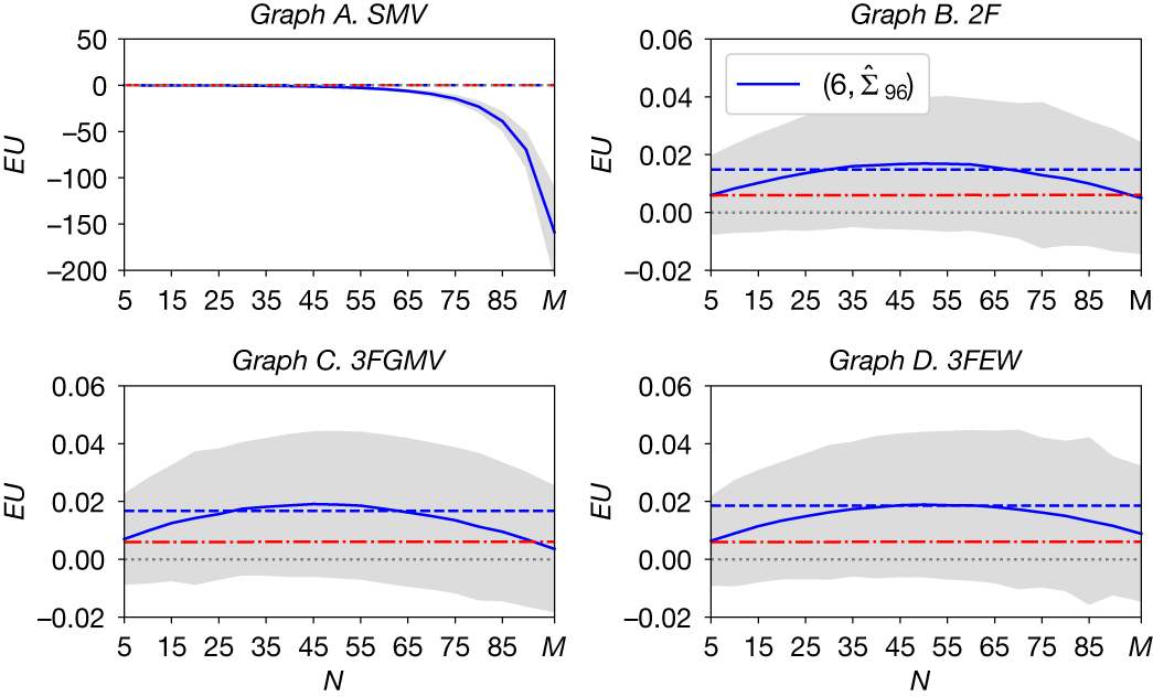


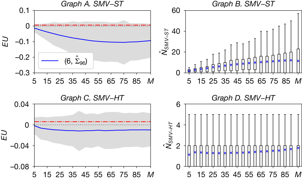


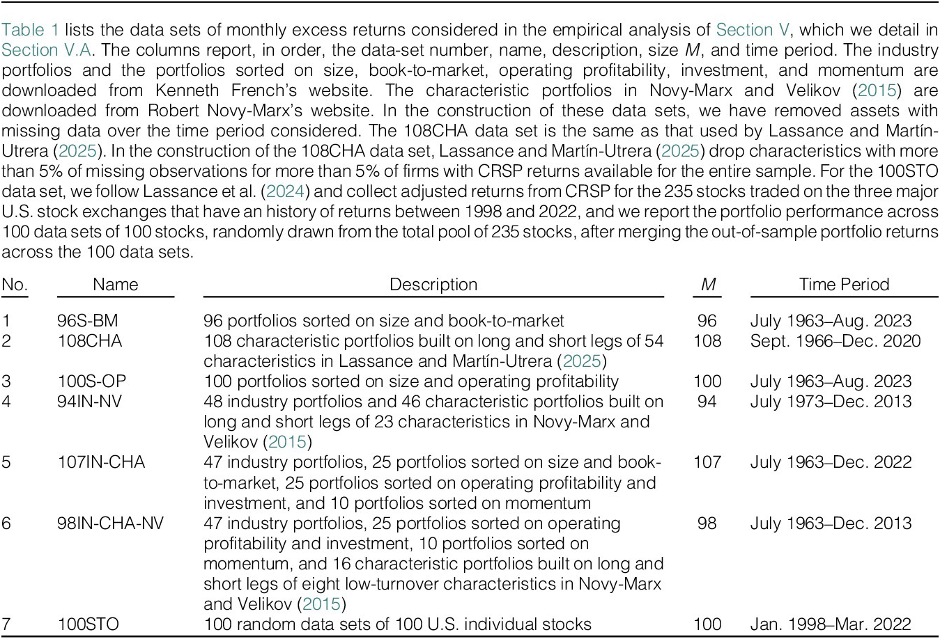
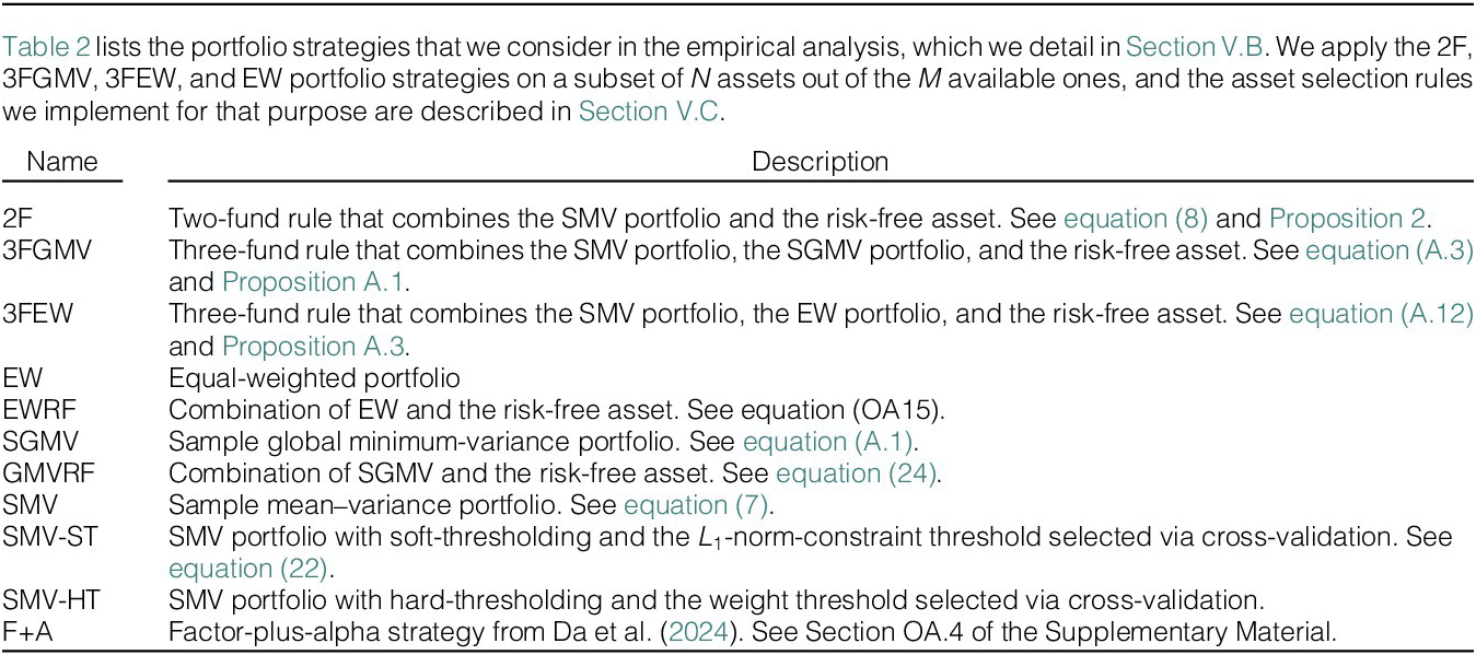
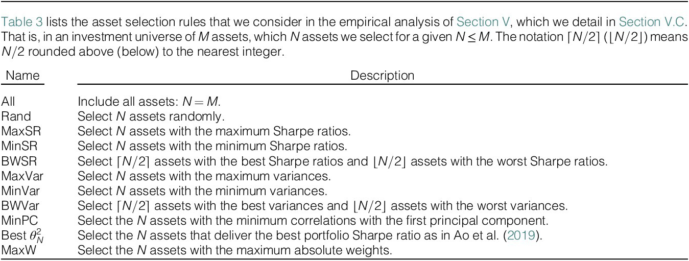
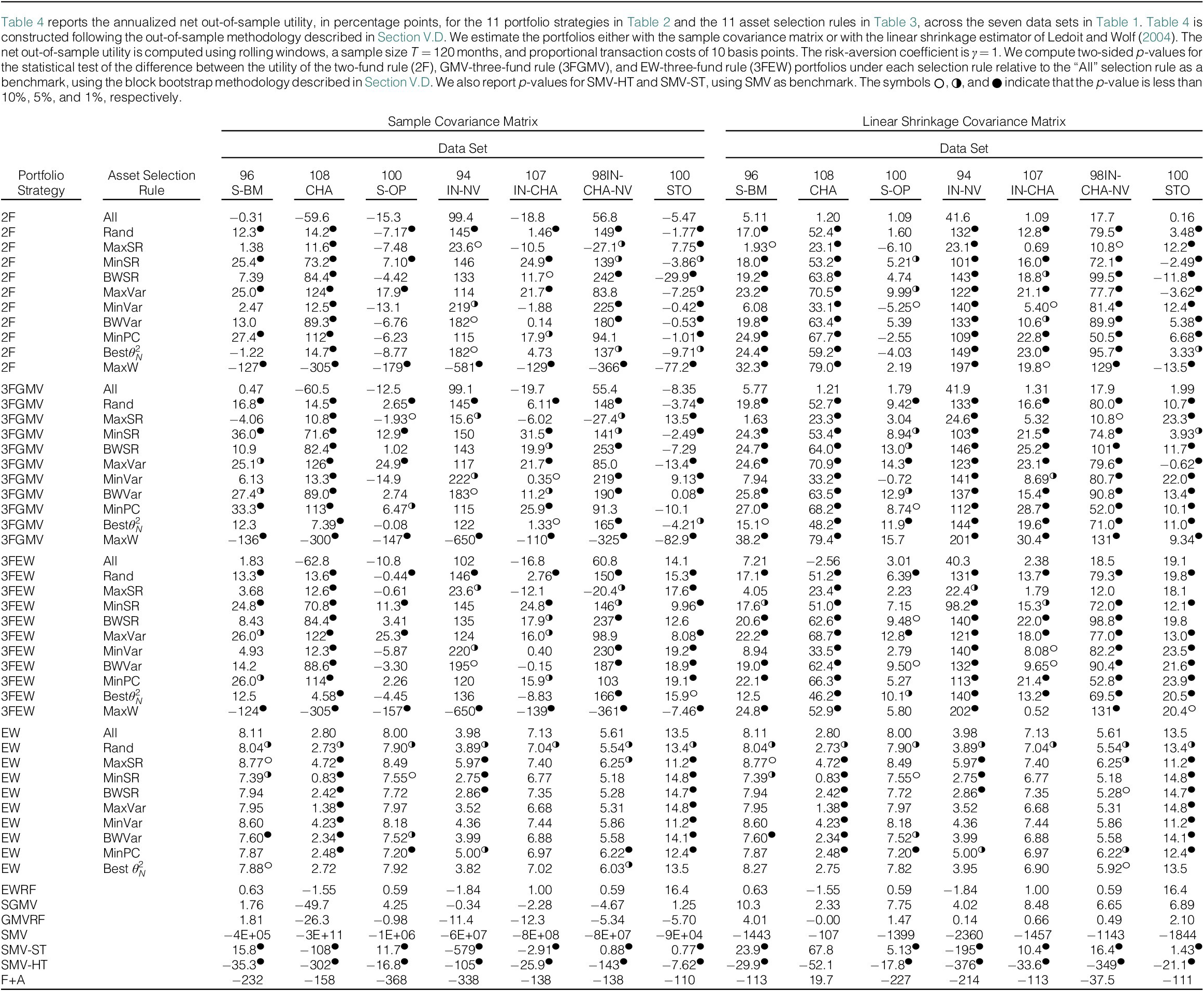
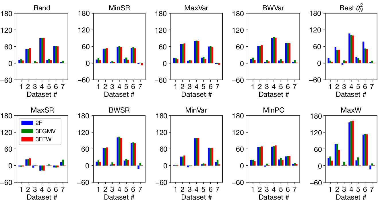


 Open access