


1. Introduction
The moving-boundary problem (Crank Reference Crank1984; Pozrikidis Reference Pozrikidis1997; Fokas & Kalimeris Reference Fokas and Kalimeris2017) plays a pivotal role in understanding various natural processes and engineering applications where boundaries between different phases of matter or regions evolve. A prominent example of this is the Stefan problem, the simplest form (Voller, Swenson & Paola Reference Voller, Swenson and Paola2004; Mitchell & Vynnycky Reference Mitchell and Vynnycky2009; Nandi & Sanyasiraju Reference Nandi and Sanyasiraju2020) of which involves a partial differential equation for energy transport and a dynamic boundary. For example, in heat conduction problems, the phase change between solid and liquid phases creates a boundary that moves as the system evolves. The complexity of these problems arises from the need to model both the evolution of the boundary and the physical processes within the domain, such as heat diffusion or mass transfer, which are often nonlinear and coupled with the dynamics of the boundary itself. While this provides a simple framework for modelling phase changes, real-world systems are often more complex, requiring modifications to account for factors such as fluid movement or external disturbances. In many practical cases (Stern Reference Stern1975; Stevens Reference Stevens2005; McPhee Reference McPhee2008), the involved phase-change material does not remain stationary but instead experiences convection due to energy gradients, buoyancy effects or external forces. The phase change in this case is driven not only by the energy diffusion but also by the convective flow within the liquid. This presents often more significant challenges both in mathematical modelling and physical understanding of the system, as it demands coupling of the flow fields with the energy transport mechanisms governed by convection–diffusion-type equations, alongside the evolving boundary. One particular class of such problems arises in the context of dissolution processes (Davies Wykes et al. Reference Wykes, Megan, Huang, Hajjar and Ristroph2018; Ristroph Reference Ristroph2018; Pegler & Davies Wykes Reference Pegler, Wykes and Megan2020; Wells & Worster Reference Wells and Worster2011; Miao, Yuan & Zhao Reference Miao, Yuan and Zhao2020; Nandi & Yedida Reference Nandi and Yedida2023), where a solute material dissolves into a surrounding fluid.
Over the years, convective dissolution phenomena have been studied across various contexts in the literature, focusing on different aspects such as the shape evolution of dissolving materials (Pegler & Davies Wykes Reference Pegler, Wykes and Megan2020, Reference Pegler, Wykes and Megan2021; Huang & Moore Reference Mac Huang and Moore2022), employment of scaling laws (Huang, Moore & Ristroph Reference Huang, Moore and Ristroph2015; Dietrich et al. Reference Dietrich, Wildeman, Visser, Hofhuis, Kooij, Zandvliet and Lohse2016; Cohen et al. Reference Cohen, Berhanu, Derr and du Pont Courrech2020), flow regime analysis with their impact on the process (Sullivan, Liu & Ecke Reference Sullivan, Liu and Ecke1996; Huang, Shelley & Stein Reference Huang, Shelley and Stein2021; Nandi & Yedida Reference Nandi and Yedida2023) and so on. Despite their apparent diversity across different systems, the physical mechanisms driving these dissolution processes are governed by common underlying principles. In many cases, the dissolution of a solute into a surrounding fluid yields local variations in solute concentration, which subsequently change the fluid’s density. This density variation is the primary mechanism for the formation of convective flow as the system seeks to restore mass equilibrium. The buoyant forces caused by the density gradients lead to natural convection, which significantly affects the dissolution rate and the overall shape of the dissolving boundary. In many practical situations, in addition to these internal, naturally driven forces, external factors such as temperature gradients, shear forces, pressure gradients or external flow fields can also play a significant role in influencing the convective dissolution process. For instance, temperature gradients (Olivella et al. Reference Olivella, Carrera, Gens and Alonso1996; Naviaux et al. Reference Naviaux, Subhas, Rollins, Dong, Berelson and Adkins2019) or pressure changes (Tasaka et al. Reference Tasaka, Sekiguchi, Urahama, Matsubara, Kiyono and Suzuki1990; Ren et al. Reference Ren, Hao, Li, Wang, Liu and Li2024) can modify the dissolution dynamics by affecting both the fluid’s properties and the solubility of the material. Similarly, rotation of the fluid or the presence of mechanical stirring generates shear forces (Khoury, Mauger & Howard Reference Khoury, Mauger and Howard1988; Wallin & Bjerle Reference Wallin and Bjerle1989; Ashokbhai et al. Reference Ashokbhai, Sanjay, Sah and Kaity2024) within the fluid, which can enhance mixing and disturb the formation of concentration gradients near the dissolving material. However, the combined effect of these factors, along with the internal forces, determines the overall efficiency of the dissolution process.
The process driven by the interplay between internal forces with rotational factors is particularly relevant in various industrial applications such as drug dissolution, mixing processes and solute extraction from materials. Most of the studies found in the existing literature on this area are based on experimental results. For example, one may refer to the study on the dissolution of limestone in a rotating cylinder (Wallin & Bjerle Reference Wallin and Bjerle1989), dissolution of hydrocortisone alcohol and acetate in rotating fluids (Khoury et al. Reference Khoury, Mauger and Howard1988), a rotating cylinder electrode (Gabe Reference Gabe1974), and so on. In many of these studies, the typical set-up consists of a dissolvable solute placed in a rotating vertical cylindrical container filled with solvent. On the other hand, in the current study, though we focus on understanding a similar dissolution process, apart from the solute being in the shape of a circular cylinder, such as a candle or rod, the rotating cylindrical container is horizontal, rather than vertical. A previous study on the dissolution in a similar configuration but without rotation was conducted by Nandi & Yedida (Reference Nandi and Yedida2023). They mainly focused on the dissolution rate and shape evolution under various parameters like fluid–solute volumetric ratio, Stefan number $(St)$
, solutal Rayleigh number
$(St)$
, solutal Rayleigh number $(Ra)$
, Schmidt number
$(Ra)$
, Schmidt number $(Sc)$
, etc. However, this study specifically aims to examine the contribution of rotational forces to the dissolution process while keeping all other involved parameters constant. Our objective is to observe how the rate of dissolution differs with the addition of rotational force, along with the corresponding flow behaviours and shape dynamics of the solute. Additionally, the study attempts to predict dissolution time at various rotation speeds and explores the relationship between the percentage of dissolution and time. It also focuses on providing a rough/estimated idea of shape dynamics by introducing a modified Rayleigh number
$(Sc)$
, etc. However, this study specifically aims to examine the contribution of rotational forces to the dissolution process while keeping all other involved parameters constant. Our objective is to observe how the rate of dissolution differs with the addition of rotational force, along with the corresponding flow behaviours and shape dynamics of the solute. Additionally, the study attempts to predict dissolution time at various rotation speeds and explores the relationship between the percentage of dissolution and time. It also focuses on providing a rough/estimated idea of shape dynamics by introducing a modified Rayleigh number $(Ra_{\varOmega })$
that accounts for both gravitational and rotational effects. In the process, it also aims to provide a complete numerical framework for predicting the dissolution dynamics in rotating systems, which is lacking in the existing literature.
$(Ra_{\varOmega })$
that accounts for both gravitational and rotational effects. In the process, it also aims to provide a complete numerical framework for predicting the dissolution dynamics in rotating systems, which is lacking in the existing literature.
Mathematically, modelling dissolution (phase-change) systems chosen for the present configuration is fraught with unique challenges due to the dynamic nature of the interface and the additional mechanical rotational factors introduced by the rotation of the cylinder. Traditional numerical techniques often fail to adequately address such complex, time-dependent and multi-dimensional systems. This study adopts a stable and accurate boundary-fitted grid-based method (Nandi & Sanyasiraju Reference Nandi and Sanyasiraju2022), which is capable of solving the coupled nonlinear governing equations while accurately capturing the transient interface without the need for supplementary tools such as level-set, phase field, immersed boundary methods, etc. Here, at each time step of computation, the physical domain is transformed into a fixed rectangular domain using a boundary-fitted transformation. The transformed energy transport and the flow-field equations are then solved on the computational grid using an unconditionally stable alternating direction implicit (ADI) scheme, while the boundary update equations are solved using a total variation diminishing Runge–Kutta method. Before applying this numerical approach to the problem under consideration, it is validated by solving a benchmark problem of natural convective heat transfer in a counter-rotating cylindrical annulus (Abu-Sitta et al. Reference Abu-Sitta, Khanafer, Vafai and Al-Amiri2007) but without phase transition using the same scheme.
The outline of the paper is as follows. Section 2 details the mathematical formulation of the problem, including the governing equations and boundary conditions. Section 3 discusses the numerical methods used for solving the problem, while § 4 presents and analyses the results of our simulations. Finally, in § 5, we conclude by summarising our findings and suggesting potential directions for future research.
2. Mathematical model
Consider the dissolution of a cylindrical solvable substance (solid/solute) in a solvent (fluid) filling an infinitely long horizontal concentric cylinder rotating in the clockwise direction about its axis (see figure 1). As the solid dissolves, the fluid–solid boundary (interface) recedes, dissolved solute mixes with the solvent and forms a solution (solvent + dissolved solute). It is assumed that the solute is sufficiently solid so that it dissolves uniformly in the solvent without fragmenting under the influence of the developed flow. In general, the fragmentation of a dissolving substance depends on several factors, including mechanical stress from high fluid velocities, chemical instability or reactivity in the solvent, solubility limits, thermal effects and so on. Solute dissolution leads to a density gradient in the fluid, leading to a convective flow.
Further, we assume that the cylinder experiences a clockwise rotation relative to the solute at an angular velocity $\varOmega _0$
about its horizontal axis. Although the rotation of the cylinder enhances the convective flow, the assumptions of the flow remain valid up to a certain rotation speed until the solubility limit is maintained. It is worth mentioning that due to the mechanically induced forced convection resulting from cylinder rotation, the solute dissolution is driven by the combined effects of natural and forced convection.
$\varOmega _0$
about its horizontal axis. Although the rotation of the cylinder enhances the convective flow, the assumptions of the flow remain valid up to a certain rotation speed until the solubility limit is maintained. It is worth mentioning that due to the mechanically induced forced convection resulting from cylinder rotation, the solute dissolution is driven by the combined effects of natural and forced convection.
Assuming that the flow remains invariant along the axis of the cylinder, the problem can be modelled mathematically in two space dimensions. We consider a cross-section of the cylinder perpendicular to its axis such that the liquid region is contained between the cylinder and the interface (see figure 1 b for the initial time and figure 1 c for a later time). We restrict our study to the fluid region, and the boundary concentration of the solute is assumed to be equal to the phase-change concentration at which the solution saturates. Solute dissolution may generate latent heat due to the interactions between the solute and solvent molecules. Depending on the nature of the solute–solvent interactions, it may either absorb or release latent heat. However, the effects of the latent heat generated and heat arising due to mixing during the dissolution are extremely negligible on the flow structure, and hence they are neglected here. Thus, the density of the solution depends solely on the concentration of the dissolved solute.
Schematic representation of the problem under consideration. (a) An infinitely long rotating horizontal cylinder filled with an incompressible solvent (blue) in which a solute (yellow) in the shape of a concentric circular cylinder is placed initially (at time $t = 0$
), and (b) its
$t = 0$
), and (b) its $xy$
cross-section showing the two-dimensional nature of the problem under investigation in this study. (c) Location and geometry of the solute–solvent interface
$xy$
cross-section showing the two-dimensional nature of the problem under investigation in this study. (c) Location and geometry of the solute–solvent interface $\varGamma (t)$
at a later time (
$\varGamma (t)$
at a later time ( $t \gg 1$
) along with its initial position,
$t \gg 1$
) along with its initial position, $\varGamma (0)$
(dashed line), and the cylinder wall,
$\varGamma (0)$
(dashed line), and the cylinder wall, $\varGamma _w$
.
$\varGamma _w$
.

The fluid region, $\varSigma _{l}(t)\subset \mathbb{R}^2$
, is bounded by the rigid wall of the cylinder,
$\varSigma _{l}(t)\subset \mathbb{R}^2$
, is bounded by the rigid wall of the cylinder, $\varGamma _w$
(outer boundary), and the interface,
$\varGamma _w$
(outer boundary), and the interface, $\varGamma (t)$
(inner boundary). At
$\varGamma (t)$
(inner boundary). At $t = 0$
, the fluid region corresponds to an annular region (see figure 1
b), and as time progresses, its shape is determined by the evolving interface
$t = 0$
, the fluid region corresponds to an annular region (see figure 1
b), and as time progresses, its shape is determined by the evolving interface $\varGamma (t)$
(see figure 1
c) governed by the Stefan condition. The liquid is assumed to be incompressible, and the density variation is modelled using the Oberbeck–Boussinesq approximation. The mass balance of the dissolved solute concentration (
$\varGamma (t)$
(see figure 1
c) governed by the Stefan condition. The liquid is assumed to be incompressible, and the density variation is modelled using the Oberbeck–Boussinesq approximation. The mass balance of the dissolved solute concentration ( $c$
) is described in terms of an advection–diffusion equation. Thus, the resulting governing equations read as
$c$
) is described in terms of an advection–diffusion equation. Thus, the resulting governing equations read as
 \begin{align} \boldsymbol{\nabla } \boldsymbol{\cdot }\boldsymbol{u} &= 0, \quad \mbox{in} \quad \varSigma _{l}(t) \times (0, \infty ),{} \end{align}
 \begin{align} \frac {\partial \boldsymbol{u}}{\partial t} + (\boldsymbol{u}\boldsymbol{\cdot }\boldsymbol{\nabla }) \boldsymbol{u} &= - \frac {1}{\rho _0} \boldsymbol{\nabla \!} p + \nu {\nabla} ^2 \boldsymbol{u} + \hat {g} \beta _c c, \quad \mbox{in} \quad \varSigma _{l}(t) \times (0, \infty ), \end{align}
 \begin{align} \frac {\partial c}{\partial t} + \boldsymbol{u}\boldsymbol{\cdot }\boldsymbol{\nabla } c &= D {\nabla} ^2 c, \quad \mbox{in} \quad \varSigma _{l}(t) \times (0, \infty ), \end{align}
where $p$
represents the pressure distribution,
$p$
represents the pressure distribution, $\hat {g}$
denotes the gravitational acceleration,
$\hat {g}$
denotes the gravitational acceleration, $\rho _0 = \rho (c = 0)$
is the density of the solvent,
$\rho _0 = \rho (c = 0)$
is the density of the solvent, $\beta _c$
is the solutal mass expansion coefficient,
$\beta _c$
is the solutal mass expansion coefficient, $c_{\varGamma }$
is the concentration at the interface,
$c_{\varGamma }$
is the concentration at the interface, $\nu$
is the kinematic viscosity and
$\nu$
is the kinematic viscosity and $D$
is the mass diffusivity of the solute in the liquid. The last term on the right-hand side of (2.2) indicates the buoyancy force acting against the force of gravity. Here, we consider that gravity acts vertically downward, i.e.
$D$
is the mass diffusivity of the solute in the liquid. The last term on the right-hand side of (2.2) indicates the buoyancy force acting against the force of gravity. Here, we consider that gravity acts vertically downward, i.e. $\hat {g} = -g\hat {j}$
, where
$\hat {g} = -g\hat {j}$
, where $\hat {j}$
denotes the unit vector in the
$\hat {j}$
denotes the unit vector in the $y$
direction.
$y$
direction.
2.1. Initial and boundary conditions
The mathematical description of the problem is concluded by prescribing initial and boundary conditions. Initially, the fluid region is filled with quiescent solvent, mathematically
 \begin{equation} \boldsymbol{u}(\boldsymbol{x}, 0) = \boldsymbol{0}, \quad c(\boldsymbol{x}, 0) = 0 \qquad \mbox{in} \;\;\; \varSigma _l(0). \end{equation}
Fluid velocity at the boundaries satisfies
 \begin{equation} \boldsymbol{u} = V \hat {n}^\varGamma = (V_{\!x}, V_{\!y} ) \quad \mbox{ on } \quad \varGamma (t), \quad \quad \boldsymbol{u} = (\varOmega _0 y, -\varOmega _0 x ) \quad \mbox{ on } \quad \varGamma _w, \end{equation}
where $V_{\!x}$
and
$V_{\!x}$
and $V_{\!y}$
are the horizontal and vertical components of the interface velocity, respectively, and
$V_{\!y}$
are the horizontal and vertical components of the interface velocity, respectively, and $\hat {n}^\varGamma = (n_x^\varGamma , n_y^\varGamma )$
is the unit normal to the interface into the fluid region. Although the fluid velocity at the interface is assumed to be the same as the interface velocity, one can also use
$\hat {n}^\varGamma = (n_x^\varGamma , n_y^\varGamma )$
is the unit normal to the interface into the fluid region. Although the fluid velocity at the interface is assumed to be the same as the interface velocity, one can also use $V = 0$
(Huang et al. Reference Huang, Shelley and Stein2021). This assumption is relevant because the interface velocity is typically very small (
$V = 0$
(Huang et al. Reference Huang, Shelley and Stein2021). This assumption is relevant because the interface velocity is typically very small ( ${\sim} \boldsymbol{O}(10^{-5})$
) in dissolution problems. On the other hand, the fluid velocity at the wall
${\sim} \boldsymbol{O}(10^{-5})$
) in dissolution problems. On the other hand, the fluid velocity at the wall $\varGamma _w$
is specified based on a fixed clockwise rotation speed
$\varGamma _w$
is specified based on a fixed clockwise rotation speed $\varOmega _0 (\geqslant 0)$
. This indicates that the wall is treated as rotating with a constant angular velocity, without any acceleration or oscillation.
$\varOmega _0 (\geqslant 0)$
. This indicates that the wall is treated as rotating with a constant angular velocity, without any acceleration or oscillation.
At the interface $\varGamma (t)$
, concentration equals the saturation concentration (
$\varGamma (t)$
, concentration equals the saturation concentration ( $c_{\textit{sat}}$
) of the solution:
$c_{\textit{sat}}$
) of the solution:
 \begin{equation} c_{\varGamma } := c(\boldsymbol{x},t) = c_{\textit{sat}} \quad \mbox{ on } \quad \varGamma (t). \end{equation}
As the solute dissolves, the interface recedes as a necessary consequence of mass conservation, described by the flux balance (Wells & Worster Reference Wells and Worster2011; Pegler & Davies Wykes Reference Pegler, Wykes and Megan2021, and references therein):
 \begin{equation} \rho _s (c_s - c_{\varGamma } ) V = - \rho _0 D \boldsymbol{\nabla }c \boldsymbol{\cdot }\boldsymbol{n}^\varGamma \quad \mbox{ on } \quad \varGamma (t), \end{equation}
where $\rho _s$
is the density of the solid,
$\rho _s$
is the density of the solid, $c_s$
is the concentration of the undissolved solute and
$c_s$
is the concentration of the undissolved solute and $V$
is the normal velocity of the interface. The condition (2.7) indicates that the solute dissolution rate/speed depends on the concentration flux at the interface as well as the mass diffusivity of the solute in the solvent. Interestingly, in nature, the mass diffusivity of most solute materials is relatively low. As a result, we can expect the dissolution process to be slower than other phase-change processes, such as melting or solidification. However, the current investigation does not focus on any specific solute or solvent. At the outer boundary
$V$
is the normal velocity of the interface. The condition (2.7) indicates that the solute dissolution rate/speed depends on the concentration flux at the interface as well as the mass diffusivity of the solute in the solvent. Interestingly, in nature, the mass diffusivity of most solute materials is relatively low. As a result, we can expect the dissolution process to be slower than other phase-change processes, such as melting or solidification. However, the current investigation does not focus on any specific solute or solvent. At the outer boundary $\varGamma _w$
, we assume a Neumann condition:
$\varGamma _w$
, we assume a Neumann condition:
 \begin{equation} -\!D \boldsymbol{\nabla }c \boldsymbol{\cdot }\boldsymbol{n}^w = 0 \quad \mbox{ on } \quad \varGamma _w \end{equation}
representing no diffusive flux, wherein $\boldsymbol{n}^w$
represents a unit normal out of the fluid region.
$\boldsymbol{n}^w$
represents a unit normal out of the fluid region.
2.2. Non-dimensionalisation
Introducing the annular gap width $L$
as the characteristic length scale, we define the characteristic velocity as
$L$
as the characteristic length scale, we define the characteristic velocity as
 \begin{equation} u_c = \left ( g \beta _c L \Delta c \right )^{1/2}\!, \end{equation}
which is analogous to the free-fall velocity commonly used in natural convection, obtained by balancing the buoyancy and convective terms appearing in the momentum equation. Using this velocity scale, we render the non-dimensional variables as
 \begin{equation} \boldsymbol{x}^\prime = \frac {\boldsymbol{x}}{L},\quad t^\prime = \frac {t u_c}{L},\quad \boldsymbol{u}^\prime = \frac {\boldsymbol{u}}{u_c}, \quad p^\prime = \frac {p}{\rho u_{c}^2}, \quad c^\prime = \frac {c}{\Delta c}, \quad \mbox{ where } \quad \Delta c = \max _{t = 0}{(\lvert c - c_{\varGamma }\rvert )}. \end{equation}
The corresponding dimensionless equations read (after dropping the prime symbols)
 \begin{align} & \boldsymbol{\nabla } \boldsymbol{\cdot }\boldsymbol{u} = 0, \quad \mbox{ in } \quad \varSigma _{l}(t) \times (0, \infty ), \end{align}
 \begin{align} &\frac {\partial \boldsymbol{u}}{\partial t} + (\boldsymbol{u}\boldsymbol{\cdot }\boldsymbol{\nabla }) \boldsymbol{u} = - \boldsymbol{\nabla \!} p + \frac {1}{\textit{Re}} {\nabla} ^2 \boldsymbol{u} - c \hat {j}, \quad \mbox{ in } \quad \varSigma _{l}(t) \times (0, \infty ), \end{align}
 \begin{align} \frac {\partial c}{\partial t} + \boldsymbol{u}\boldsymbol{\cdot }\boldsymbol{\nabla } c &= \frac {1}{\textit{Pe}} {\nabla} ^2 c, \quad \mbox{ in } \quad \varSigma _{l}(t) \times (0, \infty ). \\[12pt] \nonumber \end{align}
Equations (2.11)–(2.13) are associated with the initial conditions
 \begin{equation} \boldsymbol{u}(\boldsymbol{x}, 0) = \boldsymbol{0}, \quad c(\boldsymbol{x}, 0) = 0 \quad \mbox{ in } \quad \varSigma _l(0), \end{equation}
boundary conditions
 \begin{align} & c = 1 \quad \mbox{ on } \quad \varGamma (t), \qquad \qquad \frac {\partial c}{\partial n^w} = 0 \quad \mbox{ on } \quad \varGamma _w, \end{align}
 \begin{align} & \boldsymbol{u} = V\! \hat {n^w} \quad \mbox{ on } \quad \varGamma (t), \qquad \qquad \boldsymbol{u} = (\varOmega y, -\varOmega x ) \quad \mbox{ on } \quad \varGamma _w, \end{align}
and the Stefan condition
 \begin{align} & V = \frac {St}{\textit{Pe}} \frac {\partial c}{\partial n^\varGamma } \quad \mbox{ on } \quad \varGamma (t). \end{align}
A close look into (2.11)–(2.17) yields that the convective dissolution problem can be studied in terms of four dimensionless parameters: Péclet number ( $\textit{Pe}$
), Reynolds number (
$\textit{Pe}$
), Reynolds number ( $\textit{Re}$
) (or, two derived parameters – solutal Rayleigh number (
$\textit{Re}$
) (or, two derived parameters – solutal Rayleigh number ( $Ra = \textit{Re} \boldsymbol{\cdot }\textit{Pe}$
) and Schmidt number (
$Ra = \textit{Re} \boldsymbol{\cdot }\textit{Pe}$
) and Schmidt number ( $Sc = \textit{Pe}/\textit{Re}$
)); Stefan number (
$Sc = \textit{Pe}/\textit{Re}$
)); Stefan number ( $St$
); and
$St$
); and $\varOmega$
. These parameters are defined as
$\varOmega$
. These parameters are defined as
 \begin{align} & \textit{Re} = \frac {u_c L}{\nu }, \;\; \textit{Pe} = \frac {u_c L}{D}, \;\; Ra = \frac {g \beta _c \Delta c L^3}{\nu D}, \;\; Sc = \frac {\nu }{D}, \;\; St = \frac {\rho _0 \Delta c}{\rho _s \Delta c_s}, \;\; \varOmega = \frac {\varOmega _0 L}{u_c}, \end{align}
where $\Delta c_s = c_s - c_\varGamma$
.
$\Delta c_s = c_s - c_\varGamma$
.
2.3. Stream function–vorticity formulation
The stream function–vorticity formulation of the Navier–Stokes equations in a two-dimensional domain facilitates a more comprehensive and intuitive understanding of flow mechanisms than the conventional representation using primitive variables ( $\boldsymbol{u}, p$
). In a two-dimensional Cartesian framework, the relationships between the stream function
$\boldsymbol{u}, p$
). In a two-dimensional Cartesian framework, the relationships between the stream function $(\psi )$
and vorticity
$(\psi )$
and vorticity $(\omega )$
are defined as follows:
$(\omega )$
are defined as follows:
 \begin{equation} (u,v) = \left ( \frac {\partial \psi }{\partial y}, - \frac {\partial \psi }{\partial x} \right )\!, \quad \omega = \frac {\partial v}{\partial x} - \frac {\partial u}{\partial y}, \end{equation}
where $ u,v$
denote the velocity components of the fluid in
$ u,v$
denote the velocity components of the fluid in $x,y$
directions, respectively. Using these relations, the governing flow system becomes
$x,y$
directions, respectively. Using these relations, the governing flow system becomes
 \begin{align} &\dfrac {\partial ^2 \psi }{\partial x^2} + \dfrac {\partial ^2 \psi }{\partial y^2} = - \omega , \quad \mbox{ in } \quad \varSigma _{l}(t) \times (0, \infty ), \end{align}
 \begin{align} & \dfrac {\partial \omega }{\partial t} + (\boldsymbol{u}\boldsymbol{\cdot }\boldsymbol{\nabla }) \omega = \frac {1}{\textit{Re}} {\nabla} ^2 \omega - \frac {\partial c}{\partial x}, \quad \mbox{ in } \quad \varSigma _{l}(t) \times (0, \infty ). \end{align}
The corresponding boundary conditions for $\psi$
are
$\psi$
are
 \begin{align} &\psi = 0, \quad \dfrac {\partial \psi }{\partial n^\varGamma } = V_{\!x} n_x^\varGamma + V_{\!y} n_y^\varGamma , \quad \mbox{ on } \quad \varGamma (t), \end{align}
 \begin{align} & \psi = 0, \quad \dfrac {\partial \psi }{\partial n^w} = \varOmega (x n_x^w + y n_y^w), \quad \mbox{ on } \quad \varGamma _w. \end{align}
To complete the system, boundary conditions for the vorticity $\omega$
are required to be computed from (2.20) utilising conditions (2.22) and (2.23). These are discussed/specified later.
$\omega$
are required to be computed from (2.20) utilising conditions (2.22) and (2.23). These are discussed/specified later.
2.4. Gibbs–Thomson effect
The Stefan condition (2.17) indicates that the interface velocity can be determined solely from the parameter ratio $St/\textit{Pe}$
and the concentration flux into the fluid region at the interface. Notably, this movement/velocity may also be influenced by the shape of the interface surface. In convex regions, where the local curvature exceeds the mean curvature, the interface moves more rapidly, enhancing the dissolution process. Conversely, in concave regions, the movement is steadier, resulting in a slower dissolution process. Although the initial circular interface of this model is smooth, it may develop irregularities in areas of both low and high curvature during dissolution. In such instances, it is necessary to equilibrate the interface motion between the concave and convex regions. The Gibbs–Thomson effect effectively addresses this requirement by establishing equilibrium in mass exchange between the solid and fluid regions due to interface effects. In this context, the interface velocity is adjusted as (Perez Reference Perez2005; Moore et al. Reference Moore, Ristroph, Childress, Zhang and Shelley2013; Huang et al. Reference Huang, Shelley and Stein2021)
$St/\textit{Pe}$
and the concentration flux into the fluid region at the interface. Notably, this movement/velocity may also be influenced by the shape of the interface surface. In convex regions, where the local curvature exceeds the mean curvature, the interface moves more rapidly, enhancing the dissolution process. Conversely, in concave regions, the movement is steadier, resulting in a slower dissolution process. Although the initial circular interface of this model is smooth, it may develop irregularities in areas of both low and high curvature during dissolution. In such instances, it is necessary to equilibrate the interface motion between the concave and convex regions. The Gibbs–Thomson effect effectively addresses this requirement by establishing equilibrium in mass exchange between the solid and fluid regions due to interface effects. In this context, the interface velocity is adjusted as (Perez Reference Perez2005; Moore et al. Reference Moore, Ristroph, Childress, Zhang and Shelley2013; Huang et al. Reference Huang, Shelley and Stein2021)
 \begin{equation} V = \dfrac {St}{\textit{Pe}} \dfrac {\partial c}{\partial n} - \epsilon\! \left ( \kappa - \frac {2 \pi }{S} \right ) \quad \mbox{ on } \quad \varGamma , \end{equation}
where $\epsilon$
is a smoothing term in the interface velocity to enhance numerical stability without affecting the physical dissolution process (Moore et al. Reference Moore, Ristroph, Childress, Zhang and Shelley2013; Huang et al. Reference Huang, Shelley and Stein2021). Here,
$\epsilon$
is a smoothing term in the interface velocity to enhance numerical stability without affecting the physical dissolution process (Moore et al. Reference Moore, Ristroph, Childress, Zhang and Shelley2013; Huang et al. Reference Huang, Shelley and Stein2021). Here, $\kappa$
and
$\kappa$
and $S$
represent the local curvature and total arc length of the interface, respectively. When the interface is circular, the local curvature
$S$
represent the local curvature and total arc length of the interface, respectively. When the interface is circular, the local curvature $\kappa$
is equivalent to the mean curvature given by
$\kappa$
is equivalent to the mean curvature given by $2\pi /S$
. As a result, no adjustment to the interface velocity is required for a steadily advancing circular interface.
$2\pi /S$
. As a result, no adjustment to the interface velocity is required for a steadily advancing circular interface.
3. Numerical methods
3.1. Transformed model in computational domain
The initial annular domain of the problem evolves due to the dynamic characteristics of the interface, which may lead to complex shapes. Therefore, in order to solve the problem on a uniform Cartesian grid numerically, the physical domain is transformed at every time step into a fixed unit square $([0,1]\times [0,1])$
using a boundary-fitted transformation (see figure 2). This transformation is implemented so that the physical boundaries of the problem align with the boundary curves of the
$([0,1]\times [0,1])$
using a boundary-fitted transformation (see figure 2). This transformation is implemented so that the physical boundaries of the problem align with the boundary curves of the $(\xi ,\eta )$
coordinates. In the present scenario, we map the inner boundary
$(\xi ,\eta )$
coordinates. In the present scenario, we map the inner boundary $\varGamma (t)$
(the interface) to the line
$\varGamma (t)$
(the interface) to the line $\xi = 0$
and the outer rotating wall
$\xi = 0$
and the outer rotating wall $\varGamma _w$
to the line
$\varGamma _w$
to the line $\xi = 1$
. The other two lines,
$\xi = 1$
. The other two lines, $\eta = 0$
and
$\eta = 0$
and $\eta = 1$
, act as artificial boundaries, allowing the computational domain to be defined without resorting to the use of physical boundaries.
$\eta = 1$
, act as artificial boundaries, allowing the computational domain to be defined without resorting to the use of physical boundaries.
Layout of a typical $10\times 24$
grid in the (a) physical
$10\times 24$
grid in the (a) physical $(x,y)$
domain and (b) computational
$(x,y)$
domain and (b) computational $(\xi ,\eta )$
domain.
$(\xi ,\eta )$
domain.

The corresponding Cartesian grid in the $(\xi ,\eta )$
domain is generated by solving the following equations (see Thompson, Thames & Mastin (Reference Thompson, Thames and Mastin1974) and Nandi & Sanyasiraju (Reference Nandi and Sanyasiraju2021) for further details):
$(\xi ,\eta )$
domain is generated by solving the following equations (see Thompson, Thames & Mastin (Reference Thompson, Thames and Mastin1974) and Nandi & Sanyasiraju (Reference Nandi and Sanyasiraju2021) for further details):
 \begin{align} & \alpha x_{\xi \xi } - 2\beta x_{\xi \eta } + \gamma x_{\eta \eta } + J^{2} \big (Px_{\xi } + Qx_{\eta } \big ) = 0, \end{align}
 \begin{align} & \alpha y_{\xi \xi } - 2\beta y_{\xi \eta } + \gamma y_{\eta \eta } + J^{2} \big (Py_{\xi } + Qy_{\eta } \big ) = 0, \end{align}
with
 \begin{align} &\alpha = x_{\eta }^{2} + y_{\eta }^{2}, \quad \beta = x_{\xi } x_{\eta } + y_{\xi } y_{\eta } , \quad \gamma = x_{\xi }^{2} + y_{\xi }^{2}, \quad J = x_{\xi } y_{\eta } - y_{\xi } x_{\eta }. \end{align}
Here, the functions $P$
and
$P$
and $Q$
are used to control the spacing between grid lines. To avoid the interpolation at every time step of calculations, time derivative is calculated in the
$Q$
are used to control the spacing between grid lines. To avoid the interpolation at every time step of calculations, time derivative is calculated in the $(\xi , \eta )$
domain using the following relation:
$(\xi , \eta )$
domain using the following relation:
 \begin{align} \left (\dfrac {\partial g}{\partial t}\right )_{x, y} & = \dfrac {\partial (x, y, g)}{\partial (\xi , \eta , t)}\big/ \dfrac {\partial (x, y, t)}{\partial (\xi , \eta , t)} \nonumber \\ & = \left (\dfrac {\partial g}{\partial t}\right )_{\xi , \eta } - \dfrac {(g_{\xi }y_{\eta } - g_{\eta }y_{\xi })}{J} \left (\dfrac {{\rm d}x}{{\rm d}t}\right )_{\xi , \eta } + \dfrac {(g_{\xi }x_{\eta } - g_{\eta }x_{\xi })}{J} \left (\dfrac {{\rm d}y}{{\rm d}t}\right )_{\xi , \eta }\!, \end{align}
where $g \in \{ c, \omega \}$
.
$g \in \{ c, \omega \}$
.
Using (3.4), the governing equation for the concentration field $c$
in the computational plane reads as
$c$
in the computational plane reads as
 \begin{equation} \left (\dfrac {\partial c}{\partial t}\right )_{\xi , \eta } = A c_{\xi \xi } + B c_{\xi \eta } + C c_{\eta \eta } + D c_{\xi } + E c_{\eta } - \big (u^{\xi }c_{\xi } + u^{\eta } c_{\eta } \big ), \end{equation}
where
 \begin{align} & A = \dfrac {\alpha }{J^{2}\textit{Pe}},\quad B = - \dfrac {2 \beta }{J^{2}\textit{Pe}},\quad C = \dfrac {\gamma }{J^{2}\textit{Pe}}, \nonumber\\ & D = \dfrac {P}{\textit{Pe}} - \dfrac {1}{J}\! \left (x_{\eta }\frac {{\rm d}y}{{\rm d}t} - y_{\eta } \frac {{\rm d}x}{{\rm d}t}\right ), \quad E = \frac {Q}{\textit{Pe}} - \frac {1}{J}\! \left ( y_{\xi } \frac {{\rm d}x}{{\rm d}t} - x_{\xi } \frac {{\rm d}y}{{\rm d}t}\right )\!. \end{align}
Similarly, the equation for the vorticity field can be expressed as
 \begin{equation} \left (\dfrac {\partial \omega }{\partial t}\right )_{\xi , \eta } = A_1 \omega _{\xi \xi } + B_1 \omega _{\xi \eta } + C_1 \omega _{\eta \eta } + D_1 \omega _{\xi } + E_1 \omega _{\eta } - \big(u^{\xi } \omega _{\xi } + u^{\eta } \omega _{\eta } \big) + R, \end{equation}
where
 \begin{align} & A_1 = \dfrac {\alpha }{J^{2}\textit{Re}},\quad B_1 = - \dfrac {2 \beta }{J^{2}\textit{Re}},\quad C_1 = \dfrac {\gamma }{J^{2}Re}, \quad R = - \dfrac {1}{J} ( c_\xi y_\eta - c_\eta y_\xi ), \nonumber\\ & D_1 = \dfrac {P}{\textit{Re}} - \frac {1}{J}\! \left ( x_{\eta } \frac {{\rm d}y}{{\rm d}t} - y_{\eta } \frac {{\rm d}x}{{\rm d}t}\right ), \quad E_1 = \dfrac {Q}{\textit{Re}} - \frac {1}{J}\! \left ( y_{\xi } \frac {{\rm d}x}{{\rm d}t} - x_{\xi } \frac {{\rm d}y}{{\rm d}t} \right )\!. \end{align}
Here, the contravariant fluid velocity components $u^{\xi }$
and
$u^{\xi }$
and $u^{\eta }$
in the
$u^{\eta }$
in the $\xi$
and
$\xi$
and $\eta$
directions are expressed as follows:
$\eta$
directions are expressed as follows:
 \begin{equation} u^{\xi } = \boldsymbol{u} \boldsymbol{\cdot }\boldsymbol{\nabla } \xi = \frac {\psi _\eta }{J}, \quad u^{\eta } = \boldsymbol{u} \boldsymbol{\cdot }\boldsymbol{\nabla } \eta = -\frac {\psi _\xi }{J}, \end{equation}
which satisfy the continuity equation (2.11). Therefore, in computations, techniques such as upwinding or downwinding can be applied using these contravariant components instead of Cartesian ones. This approach facilitates an accurate numerical representation of fluid flow across different coordinate systems. The stream function and the interface normal velocity in the $\xi \eta$
plane are described by
$\xi \eta$
plane are described by
 \begin{align} & \alpha \psi _{\xi \xi } - 2\beta \psi _{\xi \eta } + \gamma \psi _{\eta \eta } + J^{2} P \psi _{\xi } + J^{2}Q \psi _{\eta } = - J^{2}\omega , \end{align}
 \begin{align} & V = - \dfrac {St}{J \textit{Pe} \sqrt {\alpha }} (\alpha c_{\xi } - \beta c_{\eta } ) - \epsilon\! \left ( \kappa - \frac {2 \pi }{S} \right )\!, \quad \mbox{ on } \quad \xi =0 . \end{align}
At the artificial boundaries $\eta = 0$
and
$\eta = 0$
and $\eta = 1$
, the flow variables are periodic. On the other hand, at the other boundaries (
$\eta = 1$
, the flow variables are periodic. On the other hand, at the other boundaries ( $\xi = 0, 1$
), concentration
$\xi = 0, 1$
), concentration $c$
and stream function
$c$
and stream function $\psi$
are computed using (2.15), (2.22) and (2.23). Finally, the boundary conditions for
$\psi$
are computed using (2.15), (2.22) and (2.23). Finally, the boundary conditions for $\omega$
at these boundaries are derived from the conditions for
$\omega$
at these boundaries are derived from the conditions for $\psi$
and (3.10). For example, at the boundary
$\psi$
and (3.10). For example, at the boundary $\xi = 1$
, (2.23) yields
$\xi = 1$
, (2.23) yields
 \begin{align} & \psi _{\eta } = 0, \quad \psi _{\eta \eta } = 0, \end{align}
 \begin{align} & \psi _\xi = \dfrac {J \varOmega }{\alpha } ( xy_\eta - yx_\eta ) = p_1 \quad \text{(say)}. \end{align}
This leads to the equation for $\omega$
as follows:
$\omega$
as follows:
 \begin{equation} \omega = -\frac {1}{J^2} ( \alpha \psi _{\xi \xi } - 2\beta \psi _{\xi \eta } + J^2 P p_1 ). \end{equation}
A similar approach can be used to obtain the condition for $\omega$
at
$\omega$
at $\xi = 0$
. It is important to note that the derivatives involved in the
$\xi = 0$
. It is important to note that the derivatives involved in the $\omega$
boundary condition are computed using a five-point ghost cell technique to incorporate the specified lower-order non-zero derivative condition efficiently.
$\omega$
boundary condition are computed using a five-point ghost cell technique to incorporate the specified lower-order non-zero derivative condition efficiently.
3.2. Numerical scheme implementation for flow and concentration
While implementing the numerical scheme, the spatial derivatives are discretised using standard second-order central difference approximations, while the convection terms are approximated using a third-order QUICK scheme (Johnson & MacKinnon Reference Johnson and MacKinnon1992; Leonard Reference Leonard1995), as described below:
 \begin{equation} \big(u^{\xi } c_{\xi }\big)_{i} = \dfrac {u^{\xi }_{i} + \big\lvert u^{\xi }_{i}\big\rvert }{2} \phi ^{+} + \dfrac {u^{\xi }_{i} - \big\lvert u^{\xi }_{i}\big\rvert }{2} \phi ^{-}, \end{equation}
where
 \begin{align} & \phi ^{+} = \frac {1}{6h} \left ( \phi _{i-2} - 6\phi _{i-1} + 3\phi _{i} + 2\phi _{i+1} \right ), \end{align}
 \begin{align} & \phi ^{-} = \frac {1}{6h} \left ( -2\phi _{i-1} - 3\phi _{i} + 6\phi _{i+1} - \phi _{i+2} \right ). \end{align}
To compute the stream function $\psi$
, Poisson’s equation (3.10) is discretised with the boundary condition
$\psi$
, Poisson’s equation (3.10) is discretised with the boundary condition $\psi = 0$
at
$\psi = 0$
at $\xi = 0, 1$
. The resulting system of algebraic equations is solved using the bi-conjugate gradient-stabilised method with incomplete LU factorisation as a preconditioner, up to a convergence tolerance of
$\xi = 0, 1$
. The resulting system of algebraic equations is solved using the bi-conjugate gradient-stabilised method with incomplete LU factorisation as a preconditioner, up to a convergence tolerance of $10^{-10}$
of the residual vector. On the other hand, for the concentration
$10^{-10}$
of the residual vector. On the other hand, for the concentration $(c)$
and vorticity
$(c)$
and vorticity $(\omega )$
fields, the advection–diffusion equations (3.5) and (3.7) are split in the time direction using the ADI scheme (In’t Hout & Welfert Reference In’t Hout and Welfert2009):
$(\omega )$
fields, the advection–diffusion equations (3.5) and (3.7) are split in the time direction using the ADI scheme (In’t Hout & Welfert Reference In’t Hout and Welfert2009):
 \begin{align} &Y^{(0)} = c^{(n)} + \Delta tf(c^{(n)}), \end{align}
 \begin{align} &Y^{(1)} = Y^{(0)} + \lambda \Delta t [ f_{1}(Y^{(1)}) - f_{1}(c^{(n)}) ], \end{align}
 \begin{align} &Y^{(2)} = Y^{(1)} + \lambda \Delta t [ f_{2}(Y^{(2)}) - f_{2}(c^{(n)}) ], \end{align}
 \begin{align} &Y^{(3)} = Y^{(0)} + \zeta \Delta t [f (Y^{(2)}) - f(c^{(n)}) ], \end{align}
 \begin{align} &Y^{(4)} = Y^{(3)} + \lambda \Delta t [ f_{1}(Y^{(4)}) - f_{1}(Y^{(2)}) ], \end{align}
 \begin{align} &c^{(n+1)} = Y^{(4)} + \lambda \Delta t [ f_{2}(Y^{(5)}) - f_{2}(Y^{(2)}) ], \end{align}
where $f$
is defined as the sum of three functions:
$f$
is defined as the sum of three functions: $f_1$
, which consists of derivatives in the
$f_1$
, which consists of derivatives in the $\xi$
direction;
$\xi$
direction; $f_2$
, which involves derivatives in the
$f_2$
, which involves derivatives in the $\eta$
direction; and
$\eta$
direction; and $f_{12}$
, which includes mixed derivatives and additional terms. The constant parameters
$f_{12}$
, which includes mixed derivatives and additional terms. The constant parameters $\lambda$
and
$\lambda$
and $\zeta$
determining the stability of the ADI scheme are chosen as
$\zeta$
determining the stability of the ADI scheme are chosen as $\lambda \geqslant {1}/{2} + {\sqrt {3}}/{2}$
and
$\lambda \geqslant {1}/{2} + {\sqrt {3}}/{2}$
and $\zeta = {1}/{2}$
, which are in accordance with the stability analysis (In’t Hout & Welfert Reference In’t Hout and Welfert2009; Nandi & Sanyasiraju Reference Nandi and Sanyasiraju2021).
$\zeta = {1}/{2}$
, which are in accordance with the stability analysis (In’t Hout & Welfert Reference In’t Hout and Welfert2009; Nandi & Sanyasiraju Reference Nandi and Sanyasiraju2021).
The ADI splitting (3.18) involves six intermediate steps for computing the required variables for the next time step, comprising two explicit and four implicit steps. The internal variables $Y^{(0)}$
and
$Y^{(0)}$
and $Y^{(3)}$
can be obtained directly from the first and fourth explicit steps, respectively. The other variables
$Y^{(3)}$
can be obtained directly from the first and fourth explicit steps, respectively. The other variables $Y^{(1)},\ Y^{(2)},\ Y^{(4)}$
and
$Y^{(1)},\ Y^{(2)},\ Y^{(4)}$
and $Y^{(5)}$
are computed by solving the following four tri-diagonal systems:
$Y^{(5)}$
are computed by solving the following four tri-diagonal systems:
 \begin{align} &(I - \lambda \Delta t S_{\xi })[Y^{(1)}] = [Y^{(0)}] - \lambda \Delta t S_{\xi }[c^{(n)}] + \lambda \Delta t [B_{1}], \end{align}
 \begin{align} &(I - \lambda \Delta t S_{\eta })[Y^{(2)}] = [Y^{(1)}] - \lambda \Delta t S_{\eta }[c^{(n)}] + \lambda \Delta t [B_{2}], \end{align}
 \begin{align} & (I - \lambda \Delta t S_{\xi })[Y^{(4)}] = [Y^{(3)}] - \lambda \Delta t S_{\xi }[Y^{(2)}] + \lambda \Delta t [B_{3}], \end{align}
 \begin{align} & (I - \lambda \Delta t S_{\eta })[Y^{(5)}] = [Y^{(4)}] - \lambda \Delta t S_{\eta }[Y^{(2)}] + \lambda \Delta t [B_{4}], \end{align}
which are deduced from the remaining four implicit steps. Here, $S_\xi$
and
$S_\xi$
and $S_\eta$
are two tri-diagonal matrices derived from discretised equations involving functions
$S_\eta$
are two tri-diagonal matrices derived from discretised equations involving functions $f_{1}(c)$
and
$f_{1}(c)$
and $f_{2}(c)$
. The column vectors
$f_{2}(c)$
. The column vectors $B_{l}$
(where
$B_{l}$
(where $l = 1, \ldots , 4$
) appearing in (3.19a
–
d
) represent the boundary conditions. The boundary conditions for the variables at the intermediate time steps are treated the same as those at the working time steps.
$l = 1, \ldots , 4$
) appearing in (3.19a
–
d
) represent the boundary conditions. The boundary conditions for the variables at the intermediate time steps are treated the same as those at the working time steps.
It is worth noting that although there are four tri-diagonal systems, two distinct tri-diagonal matrices are sufficient to handle the computations for the required variables at a particular time step. The ADI scheme is preferred over other implicit or explicit methods, such as the Crank–Nicolson and total variation diminishing Runge–Kutta schemes, for solving the convection–diffusion equation for vorticity and concentration owing to the former’s computational economy and unconditional stability.
3.3. Interface tracking
Recall from § 3.1 that $\xi = 0$
corresponds to the interface. Therefore, the unit normal at the interface can be expressed as
$\xi = 0$
corresponds to the interface. Therefore, the unit normal at the interface can be expressed as $\displaystyle \boldsymbol{n}^\varGamma = ( {y_\eta }/{\sqrt {\alpha }}, - {x_\eta }/{\sqrt {\alpha }} )$
. Thus, given the normal velocity
$\displaystyle \boldsymbol{n}^\varGamma = ( {y_\eta }/{\sqrt {\alpha }}, - {x_\eta }/{\sqrt {\alpha }} )$
. Thus, given the normal velocity $V$
from (3.11), the interface in the
$V$
from (3.11), the interface in the $xy$
plane evolves according to
$xy$
plane evolves according to
 \begin{equation} \dfrac {{\rm d}x}{{\rm d}t} = \dfrac {V\! y_\eta }{\sqrt {\alpha }}, \qquad \dfrac {{\rm d}y}{{\rm d}t} = -\dfrac {V\! x_\eta }{\sqrt {\alpha }}, \end{equation}
which can be expressed in a compact form:
 \begin{equation} \dfrac {{\rm d} \boldsymbol{X}}{{\rm d}t} = \boldsymbol{g}(\boldsymbol{X}, t), \end{equation}
where $\boldsymbol{X} = (x, y)^\top$
and
$\boldsymbol{X} = (x, y)^\top$
and $\displaystyle \boldsymbol{g} = ( V\! y_\eta /\sqrt {\alpha }, -V\! x_\eta /\sqrt {\alpha } )^\top$
. Equations (3.21) are solved using the third-order total variation diminishing Runge–Kutta scheme:
$\displaystyle \boldsymbol{g} = ( V\! y_\eta /\sqrt {\alpha }, -V\! x_\eta /\sqrt {\alpha } )^\top$
. Equations (3.21) are solved using the third-order total variation diminishing Runge–Kutta scheme:
 \begin{align} & \boldsymbol{X}^{(1)} = \boldsymbol{X}^{(n)} + \Delta t \boldsymbol{g}(\boldsymbol{X}^{(n)}, t), \end{align}
 \begin{align} & \boldsymbol{X}^{(2)} = \frac {3}{4} \boldsymbol{X}^{(n)} + \frac {1}{4} X^{(1)} + \frac {\Delta t}{4} \boldsymbol{g}(\boldsymbol{X}^{(1)}, t), \end{align}
 \begin{align} & \boldsymbol{X}^{(n+1)} = \frac {1}{3} \boldsymbol{X}^{(n)} + \frac {2}{3} \boldsymbol{X}^{(2)} + \frac {2\Delta t}{3} \boldsymbol{g}(\boldsymbol{X}^{(2)}, t). \end{align}
Here, we have used the total variation diminishing Runge–Kutta method instead of the previously used ADI scheme as the ordinary differential equation system (3.20) involves only unidirectional derivative terms along the $\eta$
direction. However, it is worth noting that a first-order explicit scheme can also be used for solving these boundary update equations rather than higher-order methods, as its effects on the accuracy of the numerical solutions are negligible (Udaykumar, Mittal & Shyy Reference Udaykumar, Mittal and Shyy1999).
$\eta$
direction. However, it is worth noting that a first-order explicit scheme can also be used for solving these boundary update equations rather than higher-order methods, as its effects on the accuracy of the numerical solutions are negligible (Udaykumar, Mittal & Shyy Reference Udaykumar, Mittal and Shyy1999).
3.4. Overview of computational framework
Numerical simulations at a given time step consist of several key steps starting with grid generation using (3.1)–(3.2). Next, the stream function $\psi$
is calculated from (3.10) based on the known values of vorticity
$\psi$
is calculated from (3.10) based on the known values of vorticity $\omega$
. Following this, the fluid velocity components
$\omega$
. Following this, the fluid velocity components $u^{\xi }$
and
$u^{\xi }$
and $u^{\eta }$
are derived from (3.9) using the stream function. The boundary conditions for
$u^{\eta }$
are derived from (3.9) using the stream function. The boundary conditions for $\omega$
are then set according to (3.14). Afterward, the concentration
$\omega$
are then set according to (3.14). Afterward, the concentration $c$
and vorticity
$c$
and vorticity $\omega$
are solved separately using the ADI scheme outlined in (3.18). Once these values are obtained, the moving interface is updated using (3.20) with the computed concentration field
$\omega$
are solved separately using the ADI scheme outlined in (3.18). Once these values are obtained, the moving interface is updated using (3.20) with the computed concentration field $c$
, and the grid is regenerated to reflect the new interface location. This cycle of computation is repeated until convergence is achieved. The numerical solution is assumed to converge when the infinity norm of the absolute errors of the variables
$c$
, and the grid is regenerated to reflect the new interface location. This cycle of computation is repeated until convergence is achieved. The numerical solution is assumed to converge when the infinity norm of the absolute errors of the variables $\omega , c, x^\varGamma\!, y^\varGamma$
satisfies the specified tolerance of
$\omega , c, x^\varGamma\!, y^\varGamma$
satisfies the specified tolerance of $10^{-8}$
. Once the process converges, the flow field, concentration field and interface are all stored at the current time step.
$10^{-8}$
. Once the process converges, the flow field, concentration field and interface are all stored at the current time step.
The code validation and grid independence studies for our computations are presented in Appendices A and B, respectively. The CPU time taken to complete one cycle of computation within the convergence loop is approximately 0.6 s for $50 \times 300$
spatial grid points using MATLAB 2022b in an Intel Xeon(R) Gold 6326 processor with a clock speed of 2.90 GHz and 64 GB of RAM.
$50 \times 300$
spatial grid points using MATLAB 2022b in an Intel Xeon(R) Gold 6326 processor with a clock speed of 2.90 GHz and 64 GB of RAM.
4. Dissolution and mixing
Our primary objective is to study the combined effects of rotation and convection on dissolution and mixing. Throughout this paper, we fix $St/\textit{Pe} = 3 \times 10^{-3}$
,
$St/\textit{Pe} = 3 \times 10^{-3}$
, $Sc = 1$
,
$Sc = 1$
, $\epsilon = 5 \times 10^{-4}$
,
$\epsilon = 5 \times 10^{-4}$
, $r_i/L = 1$
and
$r_i/L = 1$
and $r_o/L = 2$
. Thus, effects of buoyancy force (
$r_o/L = 2$
. Thus, effects of buoyancy force ( $Ra$
) and rotation (
$Ra$
) and rotation ( $\varOmega$
) are studied by varying
$\varOmega$
) are studied by varying $Ra \in [10^5, 10^8]$
and
$Ra \in [10^5, 10^8]$
and $\varOmega \in [0, 2.5]$
.
$\varOmega \in [0, 2.5]$
.
4.1. Qualitative impacts of rotation and buoyancy on flow and solute dissolution
In this section, we discuss the spatio-temporal dynamics of the dissolved solute concentration and the flow field for different values of $Ra$
and
$Ra$
and $\varOmega$
. Figure 3 depicts concentration distribution overlaid by streamlines at four instances corresponding to
$\varOmega$
. Figure 3 depicts concentration distribution overlaid by streamlines at four instances corresponding to $A_d(t) = 10\,\%,\ 30\,\%,\ 60\,\% \text{ and } 90\,\%$
(where
$A_d(t) = 10\,\%,\ 30\,\%,\ 60\,\% \text{ and } 90\,\%$
(where $A_d$
corresponds to the dissolved area, defined in (B3)) for
$A_d$
corresponds to the dissolved area, defined in (B3)) for $Ra = 10^5$
and
$Ra = 10^5$
and $\varOmega = 0$
to 2 with an increment of 0.5. At the early stages (
$\varOmega = 0$
to 2 with an increment of 0.5. At the early stages ( $A_d(t)$
approximately up to 10 %), irrespective of the rotation speed considered here, dissolution and hence the phase-change process are driven by diffusion only (see the first column of figure 3). Thus, the dissolved solute is localised near the interface, and its concentration reduces as we move away from the interface and eventually decays to zero near the wall. However, rotation breaks the left–right symmetry about the vertical axis
$A_d(t)$
approximately up to 10 %), irrespective of the rotation speed considered here, dissolution and hence the phase-change process are driven by diffusion only (see the first column of figure 3). Thus, the dissolved solute is localised near the interface, and its concentration reduces as we move away from the interface and eventually decays to zero near the wall. However, rotation breaks the left–right symmetry about the vertical axis $x = 0$
, as evident from the first column of figure 3.
$x = 0$
, as evident from the first column of figure 3.
Streamlines (white contours) overlaying the concentration contours of the dissolved solute at $A_d(t) = 10\,\%$
,
$A_d(t) = 10\,\%$
, $30\,\%$
,
$30\,\%$
, $60\,\%$
and
$60\,\%$
and $90\,\%$
(left to right) for
$90\,\%$
(left to right) for $Ra = 10^5$
and
$Ra = 10^5$
and $\varOmega =$
0–2 with an increment of 0.5 (top to bottom). The corresponding colour map illustrates the concentration variations in the domain at these instances.
$\varOmega =$
0–2 with an increment of 0.5 (top to bottom). The corresponding colour map illustrates the concentration variations in the domain at these instances.

In the absence of rotation, the primary vortices, which are observed initially on either side of the solute along the horizontal central line, gradually move towards the bottom of the solute over time and remain there until the dissolution process is complete. On the other hand, with a rotation speed of $0.5$
, a primary vortex forms on the right-hand side of the solute’s surface and eventually settles there even when dissolution reaches the
$0.5$
, a primary vortex forms on the right-hand side of the solute’s surface and eventually settles there even when dissolution reaches the $90\,\%$
stage. However, at rotation speeds of
$90\,\%$
stage. However, at rotation speeds of $1,\;1.5$
and
$1,\;1.5$
and $2$
, this vortex ceases to exist after certain stages of dissolution.
$2$
, this vortex ceases to exist after certain stages of dissolution.
Figure 3 also shows that, during dissolution with no rotation, the interplay between diffusion and buoyancy-driven convection aids in developing a laminar velocity boundary layer near the interface except at the topmost part. Rotation induces an additional laminar boundary layer near the cylinder wall. The boundary layer near the interface forms due to the combined effects of buoyancy and centripetal forces. At low rotational speeds, this layer is accompanied by a primary vortex to the right of the interface. As the rotation speed increases, the vortex is pushed away from the interface and eventually disappears. As the cylinder rotates, the fluid in immediate contact with the wall is dragged along, causing the fluid at the surface to move faster than the fluid away from the surface, which leads to the development of an additional boundary layer. An increasing rotation speed induces more shear and larger velocity gradients near the wall, affecting the nature of the boundary-layer thickness.
Streamlines (white contours) overlaying the concentration contours of the dissolved solute at $A_d(t) = 10\,\%$
,
$A_d(t) = 10\,\%$
, $30\,\%$
,
$30\,\%$
, $60\,\%$
and
$60\,\%$
and $90\,\%$
(left to right) for
$90\,\%$
(left to right) for $\varOmega =$
1 and
$\varOmega =$
1 and $Ra = 10^5$
,
$Ra = 10^5$
, $10^6$
and
$10^6$
and $10^7$
(top to bottom). The corresponding colour map illustrates the concentration variations in the domain at these instances.
$10^7$
(top to bottom). The corresponding colour map illustrates the concentration variations in the domain at these instances.

Another important observation is that the flow patterns at rotation speeds greater than $1$
begin to resemble concentric circular layers around both the solute and the cylindrical wall after a certain amount of dissolution. As the rotation speed increases, the gap between these layers becomes smaller. The flow also loses its closed trajectories and tends to become more uniform and structured.
$1$
begin to resemble concentric circular layers around both the solute and the cylindrical wall after a certain amount of dissolution. As the rotation speed increases, the gap between these layers becomes smaller. The flow also loses its closed trajectories and tends to become more uniform and structured.
A similar analysis of the flow regimes is performed by varying the Rayleigh number ( $Ra$
) while keeping the rotation speed fixed at
$Ra$
) while keeping the rotation speed fixed at $\varOmega = 1$
, which corresponds to the case when the rotation-induced laminar velocity of the cylinder is the same as that of the buoyancy-induced characteristic velocity. Figure 4 depicts that the flow varies significantly as the Rayleigh number increases. For
$\varOmega = 1$
, which corresponds to the case when the rotation-induced laminar velocity of the cylinder is the same as that of the buoyancy-induced characteristic velocity. Figure 4 depicts that the flow varies significantly as the Rayleigh number increases. For $Ra \geqslant 10^6$
, flow tends to become more irregular, and dissolved solute is localised in the right half of the cylinder.
$Ra \geqslant 10^6$
, flow tends to become more irregular, and dissolved solute is localised in the right half of the cylinder.
As discussed earlier, in the absence of rotation, buoyancy causes the dissolved solute-laden heavier fluid to sink near the solute boundary and lighter fluid to rise near the cylinder, respecting mass conservation. As dissolution increases, this convective flow progressively becomes confined within the lower half of the cylinder (see supplementary movie 1 available at https://doi.org/10.1017/jfm.2025.11009). When rotation is added to the cylinder, the upward flow near the cylinder is enhanced on the left. At the early stages of the dissolution, the qualitative feature of the flow remains similar on the left, barring fluid parcels moving faster near the cylinder, supported by the clockwise rotation of the cylinder. On the other hand, on the right, the upward flow of the fluid parcels near the cylinder is opposed by the clockwise-rotating cylinder. As a result, a region of upward-moving fluid parcels is formed, confined between two regions with downward-moving fluid parcels. The former carries fluid parcels atop the undissolved solute, leading to a forced convective flow and more dissolution on the left. With increasing dissolution of the solute, the clockwise flow (on the right) near the solute becomes progressively weaker, and the solute appears to be tilted on the right. We further noticed that the clockwise flow near the solute becomes weaker as the rotation speed increases, leading to only an anticlockwise flow near the solute and a clockwise flow near the cylinder (see supplementary movies 2–4).
Overall, we notice that rotation alters the flow topology that leads to the spreading of the dissolved solute around the interface instead of being localised only in the bottom half of the cylinder ( $\varOmega = 0$
). This causes the concentration gradient near the upper part of the interface to be shallow, and, hence, the dissolution slows down.
$\varOmega = 0$
). This causes the concentration gradient near the upper part of the interface to be shallow, and, hence, the dissolution slows down.
To further explore the behaviour of the flow regimes, we trace trajectories of passive tracers released initially at the solute–fluid interface. These trajectories represent the respective pathlines of individual fluid particles coinciding with the tracer particle and reveal how the flow dynamics changes accordingly. The equations governing the trajectory of a particle $P$
with position
$P$
with position $(X_{\!P}(t), Y_{\!P}(t))$
are
$(X_{\!P}(t), Y_{\!P}(t))$
are
 \begin{equation} \dfrac {{\rm d}X_{\!P}}{{\rm d}t} = u(X_{\!P},Y_{\!P},t), \quad \dfrac {{\rm d}Y_{\!P}}{{\rm d}t} = v(X_{\!P},Y_{\!P},t), \end{equation}
where the Eulerian velocity at its location gives the Lagrangian velocity of a particle. These equations are associated with initial conditions $X_{\!P}(t = 0) = X_{\!P}^0, \; Y_{\!P}(t = 0) = Y_{\!P}^0$
.
$X_{\!P}(t = 0) = X_{\!P}^0, \; Y_{\!P}(t = 0) = Y_{\!P}^0$
.
Pathlines of two passive tracers, released initially at $(0.0745, -1.0115)$
and
$(0.0745, -1.0115)$
and $(-0.0204, -1.9441)$
, for rotation speeds ranging from
$(-0.0204, -1.9441)$
, for rotation speeds ranging from $0$
to
$0$
to $1.5$
(shown left to right with an increment of
$1.5$
(shown left to right with an increment of $0.5$
). The respective trajectories of these particles are shown in green and blue. The initial positions of the tracers are marked with open markers, while their final positions are marked with the corresponding filled markers. Arrow markers along the pathlines denote the direction of particle motion. The red contour denotes the final shape of the undissolved solute, while
$0.5$
). The respective trajectories of these particles are shown in green and blue. The initial positions of the tracers are marked with open markers, while their final positions are marked with the corresponding filled markers. Arrow markers along the pathlines denote the direction of particle motion. The red contour denotes the final shape of the undissolved solute, while $+$
represents the centre of the cylinder.
$+$
represents the centre of the cylinder.

Figure 5 shows the trajectories of two tracer particles initially placed at $(X_{\!P}^0, Y_{\!P}^0) = (0.0745$
,
$(X_{\!P}^0, Y_{\!P}^0) = (0.0745$
, $-1.0115)$
and
$-1.0115)$
and $(X_{\!P}^0, Y_{\!P}^0) = (-0.0204, -1.9441)$
for
$(X_{\!P}^0, Y_{\!P}^0) = (-0.0204, -1.9441)$
for $Ra = 10^5$
and various rotation speeds ranging from 0 to 1.5. The initial positions of the tracers are chosen judiciously to capture the key features of the flow. The former (subsequently called ‘P1’) starts near the solute, where the flow variation is primarily dominated by buoyancy. On the other hand, the latter (subsequently called ‘P2’) is released near the cylinder, where the flow is dominated by rotation. The trajectories are tracked until 90 % dissolution of the solute is achieved. In the absence of rotation, P1 is driven by natural convection and follows a trajectory vertically downward before it moves upward along the cylinder wall, whereas P2 experiences upward motion only (see supplementary movie 5).
$Ra = 10^5$
and various rotation speeds ranging from 0 to 1.5. The initial positions of the tracers are chosen judiciously to capture the key features of the flow. The former (subsequently called ‘P1’) starts near the solute, where the flow variation is primarily dominated by buoyancy. On the other hand, the latter (subsequently called ‘P2’) is released near the cylinder, where the flow is dominated by rotation. The trajectories are tracked until 90 % dissolution of the solute is achieved. In the absence of rotation, P1 is driven by natural convection and follows a trajectory vertically downward before it moves upward along the cylinder wall, whereas P2 experiences upward motion only (see supplementary movie 5).
Cylinder rotation significantly alters the particle trajectories. Particles P1 and P2 primarily traverse in the anticlockwise and clockwise directions, respectively. However, for each $\varOmega$
, we observe a unique and distinct characteristic of the particle trajectories. When buoyancy dominates rotation (
$\varOmega$
, we observe a unique and distinct characteristic of the particle trajectories. When buoyancy dominates rotation ( $\varOmega = 0.5$
), the trajectory of P1 is confined to the right half of the cylinder for the majority of the dissolution, except at a later stage when the solute shrinks significantly and the particle has to traverse a small distance to end on the left half of the cylinder. Nonetheless, it eventually ends up on the right half (filled green marker) of the cylinder after spending a small duration on the left. For the same flow parameters, P2 initially rotates in the clockwise direction in accordance with the clockwise motion of the cylinder. However, before completing a full revolution around the solute, the particle is caught in the anticlockwise-rotating fluid parcels on the right, attracting P2 towards the solute. Subsequently, the particle traverses around the solute in the anticlockwise direction and re-enters the clockwise-rotating boundary layer adjacent to the cylinder (see supplementary movie 6).
$\varOmega = 0.5$
), the trajectory of P1 is confined to the right half of the cylinder for the majority of the dissolution, except at a later stage when the solute shrinks significantly and the particle has to traverse a small distance to end on the left half of the cylinder. Nonetheless, it eventually ends up on the right half (filled green marker) of the cylinder after spending a small duration on the left. For the same flow parameters, P2 initially rotates in the clockwise direction in accordance with the clockwise motion of the cylinder. However, before completing a full revolution around the solute, the particle is caught in the anticlockwise-rotating fluid parcels on the right, attracting P2 towards the solute. Subsequently, the particle traverses around the solute in the anticlockwise direction and re-enters the clockwise-rotating boundary layer adjacent to the cylinder (see supplementary movie 6).
For $\varOmega \gt 1$
, when rotation dominates buoyancy, P1 remains confined within a neighbourhood of the initial interface position. In particular, for
$\varOmega \gt 1$
, when rotation dominates buoyancy, P1 remains confined within a neighbourhood of the initial interface position. In particular, for $\varOmega = 1.5$
, it is evident from figure 5 that the particle exhibits a cyclic motion around the solute. The broken symmetry of the trajectory is attributed to the buoyancy that causes a departure of the particle from a perfect cyclic motion. However, as
$\varOmega = 1.5$
, it is evident from figure 5 that the particle exhibits a cyclic motion around the solute. The broken symmetry of the trajectory is attributed to the buoyancy that causes a departure of the particle from a perfect cyclic motion. However, as $\varOmega$
increases, the asymmetry becomes less prominent, and the number of revolutions of the trajectory around the solute increases (not shown for brevity). See supplementary movie 7.
$\varOmega$
increases, the asymmetry becomes less prominent, and the number of revolutions of the trajectory around the solute increases (not shown for brevity). See supplementary movie 7.
Finally, for $\varOmega = 1$
, we observe that, initially, P1 follows a trajectory similar to that for
$\varOmega = 1$
, we observe that, initially, P1 follows a trajectory similar to that for $\varOmega = 0.5$
. However, instead of being confined within the right half of the cylinder, it revolves around the solute as time progresses. After a couple of revolutions around the solute, the particle is slowly pushed away from the interface by a strong buoyant force below the solute. This process continues for a while before the particle is eventually trapped within the boundary layer near the cylinder wall and traverses in the clockwise direction. As anticipated, for both
$\varOmega = 0.5$
. However, instead of being confined within the right half of the cylinder, it revolves around the solute as time progresses. After a couple of revolutions around the solute, the particle is slowly pushed away from the interface by a strong buoyant force below the solute. This process continues for a while before the particle is eventually trapped within the boundary layer near the cylinder wall and traverses in the clockwise direction. As anticipated, for both $\varOmega = 1$
and
$\varOmega = 1$
and $\varOmega = 1.5$
, P2 rotates in the clockwise direction confined within the boundary layer near the cylinder (see supplementary movie 8).
$\varOmega = 1.5$
, P2 rotates in the clockwise direction confined within the boundary layer near the cylinder (see supplementary movie 8).
The above observations of particle paths indicate that the fluid adjacent to the cylinder wall flows in the clockwise direction, while the fluid adjacent to the interface experiences an overall anticlockwise motion. For all the cases under consideration in figure 5, the pathlines are smooth, regular and do not exhibit any disorderly behaviour, a signature of laminar flow. This behaviour is particularly evident at higher rotation speeds, for which the trajectories exhibit smooth circular motions around the solute.
4.2. Quantitative impacts of rotation and buoyancy on solute transport
In this section, we quantify dissolution, mixing and interface shape due to nonlinear interactions between fluid flow and solute dissolution over a wide range of rotation speed ( $\varOmega$
) and Rayleigh number (
$\varOmega$
) and Rayleigh number ( $Ra$
).
$Ra$
).
4.2.1. Dissolution time of the solute
Our numerical experiments are carried out until the solute experiences $95\,\%$
dissolution. Using these simulated data, we predict the time required for complete solute dissolution using spline extrapolation. Table 1 lists the time for the complete dissolution for Rayleigh numbers varying by two orders of magnitude and
$95\,\%$
dissolution. Using these simulated data, we predict the time required for complete solute dissolution using spline extrapolation. Table 1 lists the time for the complete dissolution for Rayleigh numbers varying by two orders of magnitude and $\varOmega$
ranging from 0 to 1.5. Interestingly, rotation-induced forced convection does not enhance dissolution. Rather, for a fixed Rayleigh number, the dissolution process slows down as the rotation speed increases due to a shallow concentration gradient at the interface. We further note, for
$\varOmega$
ranging from 0 to 1.5. Interestingly, rotation-induced forced convection does not enhance dissolution. Rather, for a fixed Rayleigh number, the dissolution process slows down as the rotation speed increases due to a shallow concentration gradient at the interface. We further note, for $Ra = 10^5$
and
$Ra = 10^5$
and $10^6$
, a rotation speed
$10^6$
, a rotation speed $\varOmega = 1.5$
can significantly delay the complete dissolution of the solute with an almost 85 %–94 % increase in complete dissolution as compared with the case at
$\varOmega = 1.5$
can significantly delay the complete dissolution of the solute with an almost 85 %–94 % increase in complete dissolution as compared with the case at $\varOmega = 0$
. Whereas, for
$\varOmega = 0$
. Whereas, for $Ra = 10^7$
, the time taken for complete dissolution with
$Ra = 10^7$
, the time taken for complete dissolution with $\varOmega = 1.5$
increases only up to 8 %–9 % relative to the case of no rotation. In summary, the relative strength of rotation to buoyancy plays a critical role in determining the dissolution of the solute. It appears that there exists a critical rotation speed
$\varOmega = 1.5$
increases only up to 8 %–9 % relative to the case of no rotation. In summary, the relative strength of rotation to buoyancy plays a critical role in determining the dissolution of the solute. It appears that there exists a critical rotation speed $\varOmega _{\textit{cric}}(Ra)$
such that for
$\varOmega _{\textit{cric}}(Ra)$
such that for $\varOmega \lt \varOmega _{\textit{cric}}(Ra)$
, dissolution has a weak dependence on rotation. Our prediction further indicates that
$\varOmega \lt \varOmega _{\textit{cric}}(Ra)$
, dissolution has a weak dependence on rotation. Our prediction further indicates that $\varOmega _{\textit{cric}}$
increases with
$\varOmega _{\textit{cric}}$
increases with $Ra$
.
$Ra$
.
Time required for solute dissolution at various Rayleigh numbers and rotation speeds.

Concentration of dissolved and undissolved solute in the absence of rotation and buoyancy: (a) initially ( $t = 0$
) and (b) at a later time (
$t = 0$
) and (b) at a later time ( $t \gt 0$
). Dissolution recedes the interface (red) radially. Due to this rotational symmetry, the Stefan problem associated with the dissolution can be studied through a one-dimensional model. (c) The concentration profile in the radial direction is shown from top to bottom at
$t \gt 0$
). Dissolution recedes the interface (red) radially. Due to this rotational symmetry, the Stefan problem associated with the dissolution can be studied through a one-dimensional model. (c) The concentration profile in the radial direction is shown from top to bottom at $t = 0$
,
$t = 0$
, $t = 7.5$
(early time),
$t = 7.5$
(early time), $t = 30$
(intermediate time) and
$t = 30$
(intermediate time) and $t = 60$
(later time).
$t = 60$
(later time).

We now aim to theoretically estimate a relationship for the solute dissolution time. To achieve this, we first consider a scenario where the effects of buoyancy and rotational forces are neglected. In such cases, the chosen problem is driven solely by diffusion forces, which reduces it to a classical one-dimensional phase-change problem in the radial direction due to the symmetric nature of the system. Let $r_s(t)$
and
$r_s(t)$
and $r_d(t)$
denote the radius of the undissolved solute and the distance traversed by the solid–liquid interface from its initial position, respectively, at an instantaneous time
$r_d(t)$
denote the radius of the undissolved solute and the distance traversed by the solid–liquid interface from its initial position, respectively, at an instantaneous time $t$
(see figure 6). Thus, we have
$t$
(see figure 6). Thus, we have
 \begin{equation} r_d(t) + r_s(t) = 1 \quad \text{with} \quad r_d(0) = 0 \quad \text{and} \quad r_s(0) = 1. \end{equation}
Overall, the problem can be viewed as the dissolution of a solute block in a fluid, with an expanding fluid region. Resorting to $c(r = r_d(t), t) = 1$
and following the analysis of Stefan (Reference Stefan1891), we obtain
$c(r = r_d(t), t) = 1$
and following the analysis of Stefan (Reference Stefan1891), we obtain $r_d(t)\propto \sqrt {t}$
. Thus, from (4.2) we derive
$r_d(t)\propto \sqrt {t}$
. Thus, from (4.2) we derive
 \begin{equation} 1-r_s(t) = k \sqrt {t} \quad \mbox{which yields} \quad A_d(t) = 2k\sqrt {t} - k^2t, \end{equation}
where $k$
is a constant of proportionality. The above-mentioned scaling relation is valid until the dissolved solute reaches the cylinder wall. Therefore, in the present study, the finite-size effect of the fluid region leads to a breakdown of the said power-law behaviour. We performed numerical simulations by neglecting buoyancy and rotation in our model formulation and determined the interface evolution, which agrees excellently with
$k$
is a constant of proportionality. The above-mentioned scaling relation is valid until the dissolved solute reaches the cylinder wall. Therefore, in the present study, the finite-size effect of the fluid region leads to a breakdown of the said power-law behaviour. We performed numerical simulations by neglecting buoyancy and rotation in our model formulation and determined the interface evolution, which agrees excellently with $k \sqrt {t}$
for
$k \sqrt {t}$
for $k = 0.08$
(correct up to two decimal places) up to
$k = 0.08$
(correct up to two decimal places) up to $t \lesssim 30$
(see figure 7
a).
$t \lesssim 30$
(see figure 7
a).
Time required for the gradual dissolution of the solute: (a) without buoyancy or rotation, (b) for various rotation speeds at a fixed Rayleigh number $Ra \approx 10^5$
and (c) for various Rayleigh numbers at fixed rotation speed
$Ra \approx 10^5$
and (c) for various Rayleigh numbers at fixed rotation speed $\varOmega = 1$
. Solid curves represent numerical results up to 90 % dissolution. The dashed line, proportional to
$\varOmega = 1$
. Solid curves represent numerical results up to 90 % dissolution. The dashed line, proportional to $\sqrt {t}$
, is shown as a guide to the eye. Square markers denote the predicted time for complete dissolution given in table 1.
$\sqrt {t}$
, is shown as a guide to the eye. Square markers denote the predicted time for complete dissolution given in table 1.

Effects of $Ra$
and
$Ra$
and $\varOmega$
on the evolution of
$\varOmega$
on the evolution of $r_d(t)$
and hence
$r_d(t)$
and hence $A_d(t)$
are investigated next. We numerically compute
$A_d(t)$
are investigated next. We numerically compute $A_d(t)$
, defined in (B3), for different values of
$A_d(t)$
, defined in (B3), for different values of $Ra$
and
$Ra$
and $\varOmega$
. For a fixed
$\varOmega$
. For a fixed $Ra$
, the evolution of
$Ra$
, the evolution of $A_d(t)$
is independent of
$A_d(t)$
is independent of $\varOmega$
at the early stages of the dissolution. For example, with
$\varOmega$
at the early stages of the dissolution. For example, with $Ra = 10^5$
, the effects of rotation become evident at
$Ra = 10^5$
, the effects of rotation become evident at $A_d(t) \gtrsim 0.25$
(see figure 7
b). Provided the evolution of the dissolved solute area satisfies the relation (4.3), one infers that
$A_d(t) \gtrsim 0.25$
(see figure 7
b). Provided the evolution of the dissolved solute area satisfies the relation (4.3), one infers that $k$
depends on
$k$
depends on $\varOmega$
in such a way that with increasing
$\varOmega$
in such a way that with increasing $\varOmega$
,
$\varOmega$
, $k^2 t$
is dominated by
$k^2 t$
is dominated by $2 k \sqrt {t}$
in (4.3). This is attributed to the fact that at higher rotation speeds, the rotation-induced effects dominate, and the buoyancy effect becomes negligible, causing the system to behave more like a purely diffusion-driven problem. On the other hand, for a fixed
$2 k \sqrt {t}$
in (4.3). This is attributed to the fact that at higher rotation speeds, the rotation-induced effects dominate, and the buoyancy effect becomes negligible, causing the system to behave more like a purely diffusion-driven problem. On the other hand, for a fixed $\varOmega$
, the effects of
$\varOmega$
, the effects of $Ra$
are evident throughout the dissolution process. However, the overall evolution of
$Ra$
are evident throughout the dissolution process. However, the overall evolution of $A_d(t)$
can be described by a power-law relation
$A_d(t)$
can be described by a power-law relation $A_d(t) \sim t^a$
, for
$A_d(t) \sim t^a$
, for $a \in (0.5278, 0.6354)$
.
$a \in (0.5278, 0.6354)$
.
In an attempt to explain this nonlinear dependence on $Ra$
and
$Ra$
and $\varOmega$
, we revisit the non-dimensional parameters
$\varOmega$
, we revisit the non-dimensional parameters $Ra$
and
$Ra$
and $\varOmega$
. In a forced convection, the velocity field is proportional to
$\varOmega$
. In a forced convection, the velocity field is proportional to $\varOmega$
. Thus, we write
$\varOmega$
. Thus, we write
 \begin{equation} \textit{Re} \sim \varOmega , \quad \textit{Pe} \sim \varOmega \quad \mbox{resulting in} \quad Ra \sim \varOmega ^2. \end{equation}
Subsequently, we observe that $A_d(t)$
follows a
$A_d(t)$
follows a $\sqrt {t}$
relation provided
$\sqrt {t}$
relation provided
 \begin{equation} \sqrt {Ra_{\varOmega }} \lesssim 250, \quad \mbox{where } Ra_\varOmega = \frac {Ra}{\varOmega ^2}. \end{equation}
Within this specific range for $Ra_\varOmega$
, the flow is dominated by rotation, and the interface is consistently observed to maintain its nearly initial circular shape throughout the dissolution process. On the other hand, when
$Ra_\varOmega$
, the flow is dominated by rotation, and the interface is consistently observed to maintain its nearly initial circular shape throughout the dissolution process. On the other hand, when $\sqrt {Ra_{\varOmega }} \gt 250$
, the interface loses its circular shape due to a dominant buoyancy force (see second and third rows of figure 3 and second and third panels of figure 10).
$\sqrt {Ra_{\varOmega }} \gt 250$
, the interface loses its circular shape due to a dominant buoyancy force (see second and third rows of figure 3 and second and third panels of figure 10).
4.2.2. Mixing of the dissolved solute
Here, we quantify mixing of dissolved solute in the solvent and explore the roles of buoyancy and rotation, varying $Ra$
and
$Ra$
and $\varOmega$
. The degree of mixing is defined as (Jha, Cueto-Felgueroso & Juanes Reference Jha, Cueto-Felgueroso and Juanes2011)
$\varOmega$
. The degree of mixing is defined as (Jha, Cueto-Felgueroso & Juanes Reference Jha, Cueto-Felgueroso and Juanes2011)
 \begin{equation} \chi (t) = 1 - \dfrac {\sigma ^2(t)}{\sigma ^2_{\textit{max}}}, \end{equation}
where the variance
 \begin{equation} \sigma ^2(t) = \langle c^2 \rangle - {\langle c \rangle }^2 \end{equation}
of the concentration field can be calculated in terms of the spatial average defined as
 \begin{equation} \langle \ast \rangle (t) = \int _{\varSigma _l(t)} \ast (x,y,t) \, {\rm d}x \, {\rm d}y. \end{equation}
Here, $\sigma ^2_{\textit{max}}$
represents the maximum concentration variance observed during the dissolution or mixing process. Equation (4.6) signifies that at the perfectly segregated state (
$\sigma ^2_{\textit{max}}$
represents the maximum concentration variance observed during the dissolution or mixing process. Equation (4.6) signifies that at the perfectly segregated state ( $\chi = 0$
) variance attains its maximum value; whereas, for the perfectly mixed state, at which concentration is uniform throughout the fluid region,
$\chi = 0$
) variance attains its maximum value; whereas, for the perfectly mixed state, at which concentration is uniform throughout the fluid region, $\chi = 1$
corresponds to the zero variance.
$\chi = 1$
corresponds to the zero variance.
Effects of buoyancy and rotation on the variation of the degree of mixing with the amount of dissolved solute, $A_d$
: (a)
$A_d$
: (a) $Ra = 10^5$
,
$Ra = 10^5$
, $10^6$
and
$10^6$
and $10^7$
(light to dark), without rotation (
$10^7$
(light to dark), without rotation ( $\varOmega = 0$
, solid line) and with rotation (
$\varOmega = 0$
, solid line) and with rotation ( $\varOmega = 1$
, dashed line); (b)
$\varOmega = 1$
, dashed line); (b) $\varOmega = 0.5$
,
$\varOmega = 0.5$
, $1$
and
$1$
and $2$
(light to dark) for
$2$
(light to dark) for $Ra = 10^5$
(solid line) and
$Ra = 10^5$
(solid line) and $Ra = 10^6$
(dashed line). The black line corresponds to pure diffusion, i.e. without buoyancy or rotation.
$Ra = 10^6$
(dashed line). The black line corresponds to pure diffusion, i.e. without buoyancy or rotation.

Due to the absence of dissolved solute in the fluid region initially ( $c_0(\boldsymbol{x}, 0) \equiv 0$
), spatial variance is zero and hence
$c_0(\boldsymbol{x}, 0) \equiv 0$
), spatial variance is zero and hence $\chi (0) = 1$
. As solute dissolves and mixes with the solvent,
$\chi (0) = 1$
. As solute dissolves and mixes with the solvent, $\sigma ^2(t)$
increases, resulting in
$\sigma ^2(t)$
increases, resulting in $\chi (t)$
decreasing until it reaches a local minimum,
$\chi (t)$
decreasing until it reaches a local minimum, $\chi _{\textit{min}}^{\textit{local}, 1}$
. We denote the corresponding dissolved solute area using
$\chi _{\textit{min}}^{\textit{local}, 1}$
. We denote the corresponding dissolved solute area using $A_{d, \textit{min}}^{\textit{local}, 1}$
. For
$A_{d, \textit{min}}^{\textit{local}, 1}$
. For $A_d(t) \leqslant A_{d, \textit{min}}^{\textit{local}, 1}$
,
$A_d(t) \leqslant A_{d, \textit{min}}^{\textit{local}, 1}$
, $\chi (t)$
is dominated by diffusion with a decay rate that depends on
$\chi (t)$
is dominated by diffusion with a decay rate that depends on $Ra$
and
$Ra$
and $\varOmega$
. We note that, depending on
$\varOmega$
. We note that, depending on $Ra$
and
$Ra$
and $\varOmega$
,
$\varOmega$
, $\chi (t)$
may attain the global minimum value
$\chi (t)$
may attain the global minimum value $\chi _{\textit{min}}^{\textit{global}} (= 0)$
. The smallest
$\chi _{\textit{min}}^{\textit{global}} (= 0)$
. The smallest $A_d(t)$
for which
$A_d(t)$
for which $\chi (t) = 0$
is denoted as
$\chi (t) = 0$
is denoted as $A_{d, \textit{min}}^{\textit{global}}$
. For the reference case of no rotation and buoyancy (black line in figure 8),
$A_{d, \textit{min}}^{\textit{global}}$
. For the reference case of no rotation and buoyancy (black line in figure 8), $A_{d, \textit{min}}^{\textit{local}, 1} = A_{d, \textit{min}}^{\textit{global}}$
, which may also occur for certain combinations of
$A_{d, \textit{min}}^{\textit{local}, 1} = A_{d, \textit{min}}^{\textit{global}}$
, which may also occur for certain combinations of $Ra$
and
$Ra$
and $\varOmega$
. In the absence of rotation (
$\varOmega$
. In the absence of rotation ( $\varOmega = 0$
),
$\varOmega = 0$
), $A_{d, \textit{min}}^{\textit{global}}$
increases as
$A_{d, \textit{min}}^{\textit{global}}$
increases as $Ra$
increases (solid lines in figure 8
a). On the other hand, for
$Ra$
increases (solid lines in figure 8
a). On the other hand, for $\varOmega = 1$
,
$\varOmega = 1$
, $A_{d, \textit{min}}^{\textit{global}}$
decreases as
$A_{d, \textit{min}}^{\textit{global}}$
decreases as $Ra$
increases (dashed lines in figure 8
a). However, no such correlation is obtained on varying
$Ra$
increases (dashed lines in figure 8
a). However, no such correlation is obtained on varying $\varOmega\ (\gt 0)$
for a fixed
$\varOmega\ (\gt 0)$
for a fixed $Ra$
(see figure 8
b). Evolution of
$Ra$
(see figure 8
b). Evolution of $\chi (t)$
beyond
$\chi (t)$
beyond $A_{d, \textit{min}}^{\textit{local}, 1}$
is governed by nonlinear interactions of buoyancy and rotation forces. Nonetheless, for a given
$A_{d, \textit{min}}^{\textit{local}, 1}$
is governed by nonlinear interactions of buoyancy and rotation forces. Nonetheless, for a given $Ra$
, at 90
$Ra$
, at 90 $\,\%$
dissolution of the solute, a better mixed state is obtained through rotation as compared with that in the absence of rotation (figure 8
a). Likewise, for a given rotation speed
$\,\%$
dissolution of the solute, a better mixed state is obtained through rotation as compared with that in the absence of rotation (figure 8
a). Likewise, for a given rotation speed $\varOmega$
, at 90
$\varOmega$
, at 90 $\,\%$
dissolution of the solute, a better mixed state is obtained for smaller
$\,\%$
dissolution of the solute, a better mixed state is obtained for smaller $Ra$
(figure 8
b). Thus, we conclude that there is an optimal pair of
$Ra$
(figure 8
b). Thus, we conclude that there is an optimal pair of $Ra$
and
$Ra$
and $\varOmega$
that causes the dissolved solute to mix better in the solvent.
$\varOmega$
that causes the dissolved solute to mix better in the solvent.
4.2.3. Symmetry breaking due to rotation
As discussed in § 4.1, in the absence of rotation, the dissolved solute shrinks due to buoyancy force, spreads symmetrically about the $y$
axis and primarily occupies the bottom half of the cylinder – the centre of mass of the dissolved solute is (0,
$y$
axis and primarily occupies the bottom half of the cylinder – the centre of mass of the dissolved solute is (0, $-y^\ast (t; Ra)$
). The introduction of cylinder rotation breaks this symmetry. To investigate this symmetry breaking, we compute the centre of mass of the dissolved solute as follows:
$-y^\ast (t; Ra)$
). The introduction of cylinder rotation breaks this symmetry. To investigate this symmetry breaking, we compute the centre of mass of the dissolved solute as follows:
 \begin{equation} \mu _X(t) = \int _{\varSigma _l(t)} x c_X(x,t) \, {\rm d}x, \quad \mu _Y(t) = \int _{\varSigma _l(t)} y c_Y(y,t) \, {\rm d}y, \end{equation}
where
 \begin{align} & \displaystyle c_X(x, t) = \int _{\varSigma _l(t)} c_{X,Y}(x, y,t) \, {\rm d}y, \end{align}
 \begin{align} & \displaystyle c_Y(y, t) = \int _{\varSigma _l(t)} c_{X,Y}(x, y,t) \, {\rm d}x \end{align}
and
 \begin{equation} c_{X,Y}(x, y,t) = \dfrac {c(x, y,t)}{\langle c \rangle (t)}. \end{equation}
The angular departure of the line joining ( $\mu _X(t), \mu _Y(t)$
) to the centre of the cylinder from the negative
$\mu _X(t), \mu _Y(t)$
) to the centre of the cylinder from the negative $y$
axis, measured in the counterclockwise direction, can be computed as
$y$
axis, measured in the counterclockwise direction, can be computed as
 \begin{equation} \theta (t) = \tan ^{-1}\left (\dfrac {\mu _Y(t)}{\mu _X(t)}\right ) - \frac {3\pi }{2}. \end{equation}
As anticipated, in the absence of rotation, the inclination angle is always zero (see dashed line in figure 9
a). We discuss our observations for $Ra \in \{ 10^5, 10^6, 10^7 \}$
and
$Ra \in \{ 10^5, 10^6, 10^7 \}$
and $\varOmega \in \{ 0.5, 1, 2 \}$
. For all the parameter values considered here,
$\varOmega \in \{ 0.5, 1, 2 \}$
. For all the parameter values considered here, $\theta$
remains non-negative, signifying that the centre of mass of dissolved solute always shifts to the opposite direction of rotation of the cylinder. Though the overall variation of
$\theta$
remains non-negative, signifying that the centre of mass of dissolved solute always shifts to the opposite direction of rotation of the cylinder. Though the overall variation of $\theta (t)$
with
$\theta (t)$
with $A_d(t)$
is non-monotonic, at the early stages of dissolution, growing angular departure is dominated by diffusion and rotation. As the amount of dissolved solute increases in the solvent, buoyancy forces become stronger and counter the rotation. Nonlinear interactions of these two counterbalancing forces on the spreading of the dissolved solute result in non-monotonic variations of
$A_d(t)$
is non-monotonic, at the early stages of dissolution, growing angular departure is dominated by diffusion and rotation. As the amount of dissolved solute increases in the solvent, buoyancy forces become stronger and counter the rotation. Nonlinear interactions of these two counterbalancing forces on the spreading of the dissolved solute result in non-monotonic variations of $\theta (t)$
with
$\theta (t)$
with $A_d(t)$
. Each local optimum value
$A_d(t)$
. Each local optimum value $\theta _{opt}^{local, i} \; (i = 1, 2,\ldots )$
corresponding to a specific dissolution volume
$\theta _{opt}^{local, i} \; (i = 1, 2,\ldots )$
corresponding to a specific dissolution volume $A_{d, \textit{opt}}^{local, i}$
signifies a reversal of dominance between rotation and buoyancy. To be more specific, for
$A_{d, \textit{opt}}^{local, i}$
signifies a reversal of dominance between rotation and buoyancy. To be more specific, for $A_{d, \textit{opt}}^{\textit{local}, 1} \lt A_d(t) \lt A_{d, \textit{opt}}^{\textit{local}, 2}$
buoyancy dominates rotation and
$A_{d, \textit{opt}}^{\textit{local}, 1} \lt A_d(t) \lt A_{d, \textit{opt}}^{\textit{local}, 2}$
buoyancy dominates rotation and $\theta (t)$
decreases, whereas, for
$\theta (t)$
decreases, whereas, for $A_{d, \textit{opt}}^{\textit{local}, 2} \lt A_d(t) \lt A_{d, \textit{opt}}^{\textit{local}, 3}$
, rotation dominates buoyancy and
$A_{d, \textit{opt}}^{\textit{local}, 2} \lt A_d(t) \lt A_{d, \textit{opt}}^{\textit{local}, 3}$
, rotation dominates buoyancy and $\theta {(t)}$
increases and so on.
$\theta {(t)}$
increases and so on.
Variation of the angle of inclination, $\theta (t)$
, with the dissolved volume,
$\theta (t)$
, with the dissolved volume, $A_d(t)$
: (a) fixed Rayleigh number
$A_d(t)$
: (a) fixed Rayleigh number $Ra = 10^5$
and varying rotation speed
$Ra = 10^5$
and varying rotation speed $\varOmega$
; (b) fixed
$\varOmega$
; (b) fixed $\varOmega = 1$
with varying
$\varOmega = 1$
with varying $Ra$
.
$Ra$
.

For $Ra = 10^5$
,
$Ra = 10^5$
, $A_{d, \textit{opt}}^{\textit{local}, 1}$
(
$A_{d, \textit{opt}}^{\textit{local}, 1}$
( $\theta _{opt}^{\textit{local}, 1}$
) decreases (increases) with
$\theta _{opt}^{\textit{local}, 1}$
) decreases (increases) with $\varOmega$
(see figure 9
a). On the other hand, for
$\varOmega$
(see figure 9
a). On the other hand, for $\varOmega = 1$
, both
$\varOmega = 1$
, both $A_{d, \textit{opt}}^{\textit{local}, 1}$
and
$A_{d, \textit{opt}}^{\textit{local}, 1}$
and $\theta _{opt}^{\textit{local}, 1}$
increase with
$\theta _{opt}^{\textit{local}, 1}$
increase with $Ra$
(see figure 9
b). We further note that for
$Ra$
(see figure 9
b). We further note that for $Ra = 10^5$
and
$Ra = 10^5$
and $\varOmega = 0.5$
,
$\varOmega = 0.5$
, $\theta (t)$
does not vary significantly as solute dissolves. As rotation increases
$\theta (t)$
does not vary significantly as solute dissolves. As rotation increases $(\varOmega \geqslant 1)$
, competing buoyancy and rotation forces result in a rapid oscillation in
$(\varOmega \geqslant 1)$
, competing buoyancy and rotation forces result in a rapid oscillation in $\theta$
as solute dissolves, and the frequency of oscillations increases with
$\theta$
as solute dissolves, and the frequency of oscillations increases with $\varOmega$
(see figure 9
a). At a higher rotation speed,
$\varOmega$
(see figure 9
a). At a higher rotation speed, $\theta (t)$
decreases as
$\theta (t)$
decreases as $A_d(t)$
increases, signifying a homogeneous distribution of the dissolved solute in the fluid region, which is in agreement with our observations in § 4.1.
$A_d(t)$
increases, signifying a homogeneous distribution of the dissolved solute in the fluid region, which is in agreement with our observations in § 4.1.
4.2.4. Interface evolution
This section examines how the shape of the interface evolves during the dissolution process at various rotation speeds. Figure 10 shows the interface at 15 % dissolution intervals up to 90 % for each rotation speed ranging from $0$
to
$0$
to $2$
. Irrespective of the rotation speed, the interface at the initial stages (up to 15 % dissolution) maintains its circular shape and attains different shapes at later stages depending on the resultant of the forces.
$2$
. Irrespective of the rotation speed, the interface at the initial stages (up to 15 % dissolution) maintains its circular shape and attains different shapes at later stages depending on the resultant of the forces.
The shape dynamics of the interface for rotation speeds ranging from $0$
to
$0$
to $2$
(shown from left to right with an increment of
$2$
(shown from left to right with an increment of $0.5$
) and
$0.5$
) and $Ra = 10^5$
. For each case, the positions of the interface evolutions are shown (inward with colour changing from light to dark) at every 15 % interval of dissolution with the outermost curve representing the initial interface and the innermost at 90 % dissolution. The filled black circle indicates the centre of the cylinder.
$Ra = 10^5$
. For each case, the positions of the interface evolutions are shown (inward with colour changing from light to dark) at every 15 % interval of dissolution with the outermost curve representing the initial interface and the innermost at 90 % dissolution. The filled black circle indicates the centre of the cylinder.

In the absence of rotation, the interface evolves to an egg-like shape as solute dissolves. For the same parameter values, a qualitatively similar evolution has been observed by Huang et al. (Reference Huang, Shelley and Stein2021), in which a circular solute placed at the centre of a rectangular domain developed an egg-like shape during dissolution. At these stages, it appears that the solute moves downward due to buoyancy. However, in reality, the solute does not move from its initial position; rather, the convection-induced preferential dissolution of the upper part of the solute results in an apparent movement of the solute. A similar phenomenon is observed at a lower rotation speed of the cylinder ( $\varOmega \leqslant 0.5$
). In such cases, the solute is seen to be tilted noticeably in the direction opposite to that of rotation. However, as rotation speed increases (
$\varOmega \leqslant 0.5$
). In such cases, the solute is seen to be tilted noticeably in the direction opposite to that of rotation. However, as rotation speed increases ( $\varOmega \geqslant 1$
), the interface regains its circular shape. When the cylinder rotates sufficiently fast (e.g.
$\varOmega \geqslant 1$
), the interface regains its circular shape. When the cylinder rotates sufficiently fast (e.g. $Ra = 10^5$
,
$Ra = 10^5$
, $\varOmega \geqslant 1.5$
), the interface maintains almost a perfectly circular shape exhibiting the axisymmetry of the flow and dissolution. A closer look reveals a slight asymmetry of the interface, which is in agreement with a non-zero
$\varOmega \geqslant 1.5$
), the interface maintains almost a perfectly circular shape exhibiting the axisymmetry of the flow and dissolution. A closer look reveals a slight asymmetry of the interface, which is in agreement with a non-zero $\theta$
for such cases.
$\theta$
for such cases.
The shape dynamics of the interface for $Ra = 10^5$
,
$Ra = 10^5$
, $10^6$
and
$10^6$
and $10^7$
(left to right) at a fixed rotation speed
$10^7$
(left to right) at a fixed rotation speed $\varOmega = 1.0$
. For each case, the positions of the interface evolutions are shown (inward with colour changing from light to dark) at every 15 % interval of dissolution, with the outermost curve representing the initial interface and the innermost at 90 % dissolution. The filled black circle indicates the centre of the cylinder.
$\varOmega = 1.0$
. For each case, the positions of the interface evolutions are shown (inward with colour changing from light to dark) at every 15 % interval of dissolution, with the outermost curve representing the initial interface and the innermost at 90 % dissolution. The filled black circle indicates the centre of the cylinder.

A similar analysis is of interface evolution for $\varOmega = 1$
and varying
$\varOmega = 1$
and varying $Ra \in \{ 10^5, 10^6, 10^7 \}$
indicates that the axisymmetry of the interface breaks down as the strength of the buoyancy forces (
$Ra \in \{ 10^5, 10^6, 10^7 \}$
indicates that the axisymmetry of the interface breaks down as the strength of the buoyancy forces ( $Ra$
) increases (see figure 11). As discussed in § 4.2.1, dissolution of the solute exhibits identical power-law behaviour for
$Ra$
) increases (see figure 11). As discussed in § 4.2.1, dissolution of the solute exhibits identical power-law behaviour for $R_\varOmega \lesssim 250$
. Motivated by this observation, we investigated the evolution of the interface in terms of
$R_\varOmega \lesssim 250$
. Motivated by this observation, we investigated the evolution of the interface in terms of $Ra_\varOmega$
. As discussed earlier, we have seen through several experiments that the interface always exhibits a circular shape when
$Ra_\varOmega$
. As discussed earlier, we have seen through several experiments that the interface always exhibits a circular shape when $\sqrt {Ra_{\varOmega }} \lesssim 250$
and tends to lose this shape for higher values of
$\sqrt {Ra_{\varOmega }} \lesssim 250$
and tends to lose this shape for higher values of $Ra_{\varOmega }$
. Here, we summarise the results of nine different numerical experiments in terms of three different values of the non-dimensional group
$Ra_{\varOmega }$
. Here, we summarise the results of nine different numerical experiments in terms of three different values of the non-dimensional group $Ra_\varOmega \gt 250$
.
$Ra_\varOmega \gt 250$
.
Shape dynamics of the interface at 90 % dissolution for three different modified Rayleigh numbers: (a) $\sqrt {Ra_{\varOmega }} = 1000$
, (b)
$\sqrt {Ra_{\varOmega }} = 1000$
, (b) $\sqrt {Ra_{\varOmega }} = 2000$
and (c)
$\sqrt {Ra_{\varOmega }} = 2000$
and (c) $\sqrt {Ra_{\varOmega }} = 4000$
. The filled black circle indicates the centre of the cylinder.
$\sqrt {Ra_{\varOmega }} = 4000$
. The filled black circle indicates the centre of the cylinder.

Figure 12 shows an egg-like interface for all nine cases considered here. However, the orientation of the nose (the pointed end of the egg-like shape) of the interface is primarily determined by $\varOmega$
. As expected, the same rotation speed results in a similar interface and a similar orientation of the nose of the interface. Additionally, as
$\varOmega$
. As expected, the same rotation speed results in a similar interface and a similar orientation of the nose of the interface. Additionally, as $Ra_{\varOmega }$
increases, the nose of the interface becomes sharper, exhibiting behaviour similar to the trend observed when
$Ra_{\varOmega }$
increases, the nose of the interface becomes sharper, exhibiting behaviour similar to the trend observed when $Ra$
increases, as discussed in figure 11. It is worth mentioning that the above-mentioned behaviour of the interface is limited to
$Ra$
increases, as discussed in figure 11. It is worth mentioning that the above-mentioned behaviour of the interface is limited to $Ra \lt 10^8$
, for which the overall dynamics of the flow field and the solute dissolution exhibit significantly different features, and they are briefly discussed in the next section.
$Ra \lt 10^8$
, for which the overall dynamics of the flow field and the solute dissolution exhibit significantly different features, and they are briefly discussed in the next section.
4.3. Dissolution dynamics at $Ra=10^8$

Throughout this paper, we have discussed results for the parameter ranges $10^5 \leqslant Ra \leqslant 6.4 \times 10^7$
and
$10^5 \leqslant Ra \leqslant 6.4 \times 10^7$
and $0 \leqslant \varOmega \leqslant 2.5$
, for which the flow remains regular and exhibits a laminar solutal boundary layer. We close this section by summarising numerical simulations for
$0 \leqslant \varOmega \leqslant 2.5$
, for which the flow remains regular and exhibits a laminar solutal boundary layer. We close this section by summarising numerical simulations for $Ra = 10^8$
and
$Ra = 10^8$
and $\varOmega = 0.5$
in figure 13. We observed that the interface adopts an uneven shape such that the solute region is concave. The solutal boundary layer exhibits characteristics inconsistent with laminar boundary layers (see figures 13
a and 13
b). To better understand this phenomenon, we followed the trajectories of four tracer particles – placed initially on the interface at angular locations 0,
$\varOmega = 0.5$
in figure 13. We observed that the interface adopts an uneven shape such that the solute region is concave. The solutal boundary layer exhibits characteristics inconsistent with laminar boundary layers (see figures 13
a and 13
b). To better understand this phenomenon, we followed the trajectories of four tracer particles – placed initially on the interface at angular locations 0, $\pi /2$
,
$\pi /2$
, $\pi$
and
$\pi$
and $3 \pi /2$
– as the solute dissolves. The trajectories of these tracers are captured up to 90 % of the solute dissolution and shown in figure 13(c). The loopy and relatively non-smooth particle trajectories indicate an irregular flow. Further quantification of these irregular flow dynamics is beyond the scope of the current study and will be considered in our future research.
$3 \pi /2$
– as the solute dissolves. The trajectories of these tracers are captured up to 90 % of the solute dissolution and shown in figure 13(c). The loopy and relatively non-smooth particle trajectories indicate an irregular flow. Further quantification of these irregular flow dynamics is beyond the scope of the current study and will be considered in our future research.
(a) Concentration (undissolved and dissolved solute) distribution at $0\,\%$
(initial),
$0\,\%$
(initial), $15\,\%$
,
$15\,\%$
, $30\,\%$
,
$30\,\%$
, $60\,\%$
and
$60\,\%$
and $80\,\%$
dissolution (from left to right) for
$80\,\%$
dissolution (from left to right) for $Ra=10^8$
and
$Ra=10^8$
and $\varOmega =0.5$
. In each panel, the current position of four particles released at four different positions (leftmost panel) is shown. (b) Shape of the interface at different dissolution volumes from
$\varOmega =0.5$
. In each panel, the current position of four particles released at four different positions (leftmost panel) is shown. (b) Shape of the interface at different dissolution volumes from $0\,\%$
to
$0\,\%$
to $90\,\%$
with an increment of
$90\,\%$
with an increment of $15\,\%$
(inward with colour changing from light to dark). (c) Pathlines of passive tracers released at four different positions. In each case, the brown marker represents the starting position, while the green marker indicates the position at
$15\,\%$
(inward with colour changing from light to dark). (c) Pathlines of passive tracers released at four different positions. In each case, the brown marker represents the starting position, while the green marker indicates the position at $90\,\%$
dissolution.
$90\,\%$
dissolution.

5. Summary and discussions
This work is concerned with the dissolution of a rod-shaped solute in a horizontal cylinder rotating in the clockwise direction. For low solutal Rayleigh numbers, the flow remains regular, resulting in a laminar solutal boundary layer regardless of the rotation speed. However, increasing the rotation speed renders the flow free of vorticity variation. An analysis of the dissolution time reveals that the amount of solute dissolved over time ( $A_d(t)$
) follows a power-law relation, which is determined by the balance between
$A_d(t)$
) follows a power-law relation, which is determined by the balance between $2 k \sqrt {t}$
and
$2 k \sqrt {t}$
and $k^2 t$
terms. In the absence of rotation and buoyancy, a least-squares fit to the numerical data yields
$k^2 t$
terms. In the absence of rotation and buoyancy, a least-squares fit to the numerical data yields $k \sim \boldsymbol{O}(10^{-1})$
, confirming a
$k \sim \boldsymbol{O}(10^{-1})$
, confirming a $\sqrt {t}$
evolution of
$\sqrt {t}$
evolution of $A_d(t)$
. Buoyancy and rotational convection exhibit a nonlinear influence on the amount of solute dissolved. For a fixed Rayleigh number, the square-root behaviour is maintained at higher rotation speeds. On the other hand, for a fixed rotation speed, the exponent of the power law of the relation ranges between 0.5378 to 0.6354 depending on the Rayleigh number.
$A_d(t)$
. Buoyancy and rotational convection exhibit a nonlinear influence on the amount of solute dissolved. For a fixed Rayleigh number, the square-root behaviour is maintained at higher rotation speeds. On the other hand, for a fixed rotation speed, the exponent of the power law of the relation ranges between 0.5378 to 0.6354 depending on the Rayleigh number.
During the dissolution process, as the rotation speed increases, the centre of mass of the dissolved solute moves upward, countered by the buoyancy forces. For sufficiently large rotation speed, the dissolved solute is spread uniformly within the fluid region, bringing the centre of mass to move downward and located at a place close to the case for which diffusion is the only force responsible for the dissolution. On the other hand, for a fixed moderate rotation speed, as $Ra$
increases, the centre of mass moves further away from the corresponding no rotation case. Similar to the dissolution of the solute, mixing of the dissolved solute in the solvent depends on the resultant of buoyancy and cylinder rotation. We conclude that there is an optimal pair of
$Ra$
increases, the centre of mass moves further away from the corresponding no rotation case. Similar to the dissolution of the solute, mixing of the dissolved solute in the solvent depends on the resultant of buoyancy and cylinder rotation. We conclude that there is an optimal pair of $Ra$
and
$Ra$
and $\varOmega$
that causes the dissolved solute to mix better in the solvent. Quantification of this optimal pair is beyond the scope of the current study and will be part of our future research.
$\varOmega$
that causes the dissolved solute to mix better in the solvent. Quantification of this optimal pair is beyond the scope of the current study and will be part of our future research.
As buoyancy dominates over rotational convection, the initial circular-shaped interface changes to an egg-like shape, with the pointed edge becoming increasingly sharp as $Ra$
increases. However, when rotation dominates over buoyancy, the interface nearly retains its initial circular shape throughout dissolution. A modified Rayleigh number analysis revealed that when
$Ra$
increases. However, when rotation dominates over buoyancy, the interface nearly retains its initial circular shape throughout dissolution. A modified Rayleigh number analysis revealed that when $\sqrt {Ra_\varOmega }\lesssim 250$
, the interface always retains its circular shape for any combination of
$\sqrt {Ra_\varOmega }\lesssim 250$
, the interface always retains its circular shape for any combination of $Ra\ (\lt\! 10^8)$
and
$Ra\ (\lt\! 10^8)$
and $\varOmega$
. Although their inclination with the vertical
$\varOmega$
. Although their inclination with the vertical $x$
axis was different, the interface shapes for the same
$x$
axis was different, the interface shapes for the same $Ra_\varOmega$
obtained through different combinations of
$Ra_\varOmega$
obtained through different combinations of $Ra$
and
$Ra$
and $\varOmega$
are seen to exhibit the same characteristics at any instant of dissolution.
$\varOmega$
are seen to exhibit the same characteristics at any instant of dissolution.
Although for dissolution processes $Sc$
is typically
$Sc$
is typically $\boldsymbol{O}(10^2{-}10^4)$
, here we have restricted our discussion to
$\boldsymbol{O}(10^2{-}10^4)$
, here we have restricted our discussion to $Sc = 1$
, in accordance with earlier studies in the literature (Huang et al. Reference Huang, Shelley and Stein2021; Nandi & Yedida Reference Nandi and Yedida2023). Nonetheless, additional numerical experiments for
$Sc = 1$
, in accordance with earlier studies in the literature (Huang et al. Reference Huang, Shelley and Stein2021; Nandi & Yedida Reference Nandi and Yedida2023). Nonetheless, additional numerical experiments for $Sc \geqslant 10$
yielded convergent results ensuring the robustness of our numerical scheme. Detailed quantitative analyses for
$Sc \geqslant 10$
yielded convergent results ensuring the robustness of our numerical scheme. Detailed quantitative analyses for $Sc$
relevant to some practical dissolution problems will be worth considering in future. As a general proposition, it is a compelling question to examine the relevant effects of rotation on the dissolution of a solute in the contexts of pharmaceuticals, food science, chemical engineering and environmental science, having applications in drug release into the bloodstream, ingredient dissolution in liquids, metal extraction from ores and pollutant dispersion in water. The present study paves the way to better understand the role of rotation in convective dissolution.
$Sc$
relevant to some practical dissolution problems will be worth considering in future. As a general proposition, it is a compelling question to examine the relevant effects of rotation on the dissolution of a solute in the contexts of pharmaceuticals, food science, chemical engineering and environmental science, having applications in drug release into the bloodstream, ingredient dissolution in liquids, metal extraction from ores and pollutant dispersion in water. The present study paves the way to better understand the role of rotation in convective dissolution.
Supplementary movies
Supplementary movies are available at https://doi.org/10.1017/jfm.2025.11009.
Acknowledgements
The authors thank the anonymous referees for their valuable comments and suggestions, which helped improve the quality of the paper. S.N., J.C.K. and S.P. acknowledge financial support through the Core Research Grant (CRG/2023/004156) from the Science and Engineering Research Board, Department of Science and Technology, Government of India,. S.P. acknowledges financial support through the Start-Up Research Grant (SRG/2021/001269), MATRICS Grant (MTR/2022/000493) from the Science and Engineering Research Board, Department of Science and Technology, Government of India, and Start-up Research Grant (MATHSUGIITG01371SATP002), IIT Guwahati.
Declaration of interests
The authors report no conflict of interest.
Author contributions
S.N.: Conceptualisation, Formal analysis, Investigation, Validation, Visualisation, Writing – original draft, Writing – review & editing. J.C.K.: Formal analysis, Validation, Visualisation, Writing – review & editing. S.V.S.S.Y.: Formal analysis, Validation, Writing – review & editing. S.P.: Conceptualisation, Formal analysis, Investigation, Validation, Visualisation, Writing – original draft, Writing – review & editing.
Appendix A. Validations
As a benchmark for validating the developed numerical method, we consider the classical Frank disk problem, which admits a self-similar solution describing the evolution of a moving boundary in an infinite medium. This problem, previously studied by Gibou & Fedkiw (Reference Gibou and Fedkiw2005) and Huang et al. (Reference Huang, Shelley and Stein2021), is a Stefan-type model involving temperature diffusion and interface motion without fluid convection. The temperature field $T(x,t)$
evolves according to
$T(x,t)$
evolves according to
 \begin{equation} \frac {\partial T}{\partial t} = \Delta T \quad \text{in } \varSigma _l(t), \qquad V_n = St \frac {\partial T}{\partial n} \quad \text{on } \varGamma (t), \end{equation}
with a radially symmetric interface whose exact position is given by $R(t) = S_0 \sqrt {t}$
, and the corresponding temperature distribution is
$R(t) = S_0 \sqrt {t}$
, and the corresponding temperature distribution is
 \begin{equation} T(x,t) = \begin{cases} 0, & s \leqslant S_0, \\[4pt] T_\infty \left (1 - \dfrac {F(s)}{F(S_0)}\right )\!, & s \gt S_0, \end{cases} \end{equation}
where $s = {|x|}/{\sqrt {t}}$
,
$s = {|x|}/{\sqrt {t}}$
, $F(s) = E_1 ( {s^2}/{4} )$
and
$F(s) = E_1 ( {s^2}/{4} )$
and $E_1(z) = \int _z^\infty ({{\rm e}^{-t}}/{t}) \,{\rm d}t$
is the exponential integral. Following Huang et al. (Reference Huang, Shelley and Stein2021), we set
$E_1(z) = \int _z^\infty ({{\rm e}^{-t}}/{t}) \,{\rm d}t$
is the exponential integral. Following Huang et al. (Reference Huang, Shelley and Stein2021), we set $St = -0.4$
,
$St = -0.4$
, $S_0 = 1.2$
, initial time of the numerical simulation to be
$S_0 = 1.2$
, initial time of the numerical simulation to be $t_0 = 0.1$
and an initial interface radius
$t_0 = 0.1$
and an initial interface radius $R(0.1) = 0.38$
. The far-field temperature
$R(0.1) = 0.38$
. The far-field temperature $T_\infty$
is computed from the Stefan condition using the exact solution, yielding
$T_\infty$
is computed from the Stefan condition using the exact solution, yielding $T_\infty \approx -0.999$
. The computational domain is chosen sufficiently large so that the moving interface remains well within the domain throughout the simulation up to the final time
$T_\infty \approx -0.999$
. The computational domain is chosen sufficiently large so that the moving interface remains well within the domain throughout the simulation up to the final time $t = 1$
.
$t = 1$
.
(a) Grid convergence analysis showing the relative $L^\infty$
errors in arclength and temperature with respect to the number of grid points, where the error norm is computed over all time steps. (b) Evolution of the interface at four time instances:
$L^\infty$
errors in arclength and temperature with respect to the number of grid points, where the error norm is computed over all time steps. (b) Evolution of the interface at four time instances: $t = 0.1$
,
$t = 0.1$
, $0.4$
,
$0.4$
, $0.7$
and
$0.7$
and $1.0$
, where the initial shape corresponds to
$1.0$
, where the initial shape corresponds to $t = 0.1$
. In each case, the numerical solution is shown using solid red curves and the exact interface is indicated by black dashed curves with circular markers. (c) Comparison (following the same graphical representation as (b)) of the total arclength of the interface over time from numerical simulation and the exact solution.
$t = 0.1$
. In each case, the numerical solution is shown using solid red curves and the exact interface is indicated by black dashed curves with circular markers. (c) Comparison (following the same graphical representation as (b)) of the total arclength of the interface over time from numerical simulation and the exact solution.

We provide a grid convergence analysis in figure 14(a), where five different grid configurations ( $5\times 15$
,
$5\times 15$
, $10\times 30$
,
$10\times 30$
, $20\times 60$
,
$20\times 60$
, $40\times 120$
and
$40\times 120$
and $80\times 240$
) are used to compute the relative
$80\times 240$
) are used to compute the relative $L^\infty$
errors in temperature and interface arclength. The errors are evaluated over the entire simulation time. The results indicate the accuracy of our simulation, and a grid of size
$L^\infty$
errors in temperature and interface arclength. The errors are evaluated over the entire simulation time. The results indicate the accuracy of our simulation, and a grid of size $40\times 120$
was found to be large enough to accurately capture the phenomenon. As such, we have used this grid set-up in all our subsequent simulations. Figure 14(b) illustrates the evolution of the moving interface at four different times (
$40\times 120$
was found to be large enough to accurately capture the phenomenon. As such, we have used this grid set-up in all our subsequent simulations. Figure 14(b) illustrates the evolution of the moving interface at four different times ( $t = 0.1$
,
$t = 0.1$
, $0.4$
,
$0.4$
, $0.7$
and
$0.7$
and $1.0$
), with the numerical and exact interfaces in close agreement. Figure 14(c) depicts that the time evolution of the arclength of the interface computed numerically is indistinguishable from that computed using the the exact solution, indicating the accuracy of the proposed method.
$1.0$
), with the numerical and exact interfaces in close agreement. Figure 14(c) depicts that the time evolution of the arclength of the interface computed numerically is indistinguishable from that computed using the the exact solution, indicating the accuracy of the proposed method.
Next, we consider a configuration similar to that of our primary study to further validate the numerical method. Specifically, we examine natural convective heat transfer between concentric horizontal cylinders, where the inner cylinder is heated and the annular region contains cold liquid, in the absence of moving boundaries. We first focus on the case without rotation, which has been extensively studied in the literature through experimental (Bishop, Carley & Powe Reference Bishop, Carley and Powe1968; Kuehn & Goldstein Reference Kuehn and Goldstein1976), numerical (Kuehn & Goldstein Reference Kuehn and Goldstein1976; Ingham Reference Ingham1981; Sarkar, Biswas & Öztop Reference Sarkar, Biswas and Öztop2021) and semi-analytical (Abbott Reference Abbott1964; Mack & Bishop Reference Mack and Bishop1968) approaches.
We perform a grid convergence study by comparing our numerical results with the theoretical findings of Mack & Bishop (Reference Mack and Bishop1968), who employed a power series method to solve the problem. In their approach, both the temperature and stream function were expanded in powers of the Rayleigh number. Using the first three terms of the series, the stream-function value at the stagnation point was reported as $-4.36$
for
$-4.36$
for $Ra = 3000$
,
$Ra = 3000$
, $\textit{Pr} = 0.7$
and a radius ratio
$\textit{Pr} = 0.7$
and a radius ratio $1.85$
. We compute the minimum stream-function value
$1.85$
. We compute the minimum stream-function value $\psi _{min }$
for several grid resolutions, as summarised in table 2. The results ensure convergence of the numerical results to the theoretical value, confirming the grid independence of the solution. Additionally, the average Nusselt numbers (
$\psi _{min }$
for several grid resolutions, as summarised in table 2. The results ensure convergence of the numerical results to the theoretical value, confirming the grid independence of the solution. Additionally, the average Nusselt numbers ( $\textit{Nu}$
) on both the inner and outer walls exhibited convergence across the tested grid resolutions, as shown in table 2. Based on this, we adopt a grid resolution of
$\textit{Nu}$
) on both the inner and outer walls exhibited convergence across the tested grid resolutions, as shown in table 2. Based on this, we adopt a grid resolution of $41 \times 161$
for subsequent simulations.
$41 \times 161$
for subsequent simulations.
Grid independence study for $Ra = 3000$
,
$Ra = 3000$
, $\textit{Pr} = 0.7$
and radius ratio 1.85. The minimum value of stream function (
$\textit{Pr} = 0.7$
and radius ratio 1.85. The minimum value of stream function ( $\psi _{\textit{min}}$
) and average Nusselt numbers at the inner and outer walls are shown for different grid resolutions. Results converge towards the theoretical value
$\psi _{\textit{min}}$
) and average Nusselt numbers at the inner and outer walls are shown for different grid resolutions. Results converge towards the theoretical value $\psi _{\textit{min}} = -4.36$
reported by Mack & Bishop (Reference Mack and Bishop1968).
$\psi _{\textit{min}} = -4.36$
reported by Mack & Bishop (Reference Mack and Bishop1968).

The comparison of average Nusselt number values presented in table 3 demonstrates excellent agreement between the present results and those available in the literature (Kuehn & Goldstein Reference Kuehn and Goldstein1976; Sarkar et al. Reference Sarkar, Biswas and Öztop2021). This confirms that the chosen grid resolution remains sufficiently accurate even at relatively high Rayleigh numbers. Furthermore, a qualitative comparison of streamlines and isotherms obtained using the present method with the published results of Kuehn & Goldstein (Reference Kuehn and Goldstein1976), as shown in figure 15, also revealed an excellent agreement.
Comparison of the computed average Nusselt number ( $\textit{Nu}$
) with available numerical results from the literature (Kuehn & Goldstein Reference Kuehn and Goldstein1976; Sarkar et al. Reference Sarkar, Biswas and Öztop2021) for fixed parameters values,
$\textit{Nu}$
) with available numerical results from the literature (Kuehn & Goldstein Reference Kuehn and Goldstein1976; Sarkar et al. Reference Sarkar, Biswas and Öztop2021) for fixed parameters values, $L/D_i = 0.8$
,
$L/D_i = 0.8$
, $\textit{Pr} = 0.7$
, and various Rayleigh numbers (
$\textit{Pr} = 0.7$
, and various Rayleigh numbers ( $Ra$
).
$Ra$
).

The qualitative comparison of the streamlines and isotherms obtained using the present method (second row) with the published results (Kuehn & Goldstein Reference Kuehn and Goldstein1976) (first row) for fixed $L/Di = 0.8$
. Reproduced with permission from Kuehn & Goldstein (Reference Kuehn and Goldstein1976).
$L/Di = 0.8$
. Reproduced with permission from Kuehn & Goldstein (Reference Kuehn and Goldstein1976).

We now extend the validation by considering the same annular configuration with rotational effects, which makes the set-up even closer to that of the problem considered in this study. Here, we consider the problem of heat transfer between two counter-rotating concentric cylinders for which both numerical and experimental results are available in the existing literature (Launder & Ying Reference Launder and Ying1974; Singh & Rajvanshi Reference Singh and Rajvanshi1982; Lee Reference Lee1992; Fu, Cheng & Shieh Reference Fu, Cheng and Shieh1994; Abu-Sitta et al. Reference Abu-Sitta, Khanafer, Vafai and Al-Amiri2007). The counter-rotation is achieved by rotating the inner cylinder counterclockwise with a constant angular speed $\varOmega _i$
, while the outer cylinder rotates in the clockwise direction with an angular speed
$\varOmega _i$
, while the outer cylinder rotates in the clockwise direction with an angular speed $\varOmega _o$
.
$\varOmega _o$
.
Computations are performed using $41 \times 161$
spatial grid points, which is chosen based on a grid refinement study that minimises the error in the minimum
$41 \times 161$
spatial grid points, which is chosen based on a grid refinement study that minimises the error in the minimum $(\psi _{\textit{min}})$
and maximum
$(\psi _{\textit{min}})$
and maximum $(\psi _{\textit{max}})$
values of the stream function. We compare the present numerical results with those of Abu-Sitta et al. (Reference Abu-Sitta, Khanafer, Vafai and Al-Amiri2007) for
$(\psi _{\textit{max}})$
values of the stream function. We compare the present numerical results with those of Abu-Sitta et al. (Reference Abu-Sitta, Khanafer, Vafai and Al-Amiri2007) for $R\ (:= r_o/r_i) = 2$
,
$R\ (:= r_o/r_i) = 2$
, $Re = 150$
,
$Re = 150$
, $Ra = 10^4$
,
$Ra = 10^4$
, $Pr = 0.7$
and
$Pr = 0.7$
and $\delta\ (:= \varOmega _o r_o / \varOmega _i r_i) \in \{ 0.5, 1 \}$
in table 4, which shows a consistent trend with the existing results.
$\delta\ (:= \varOmega _o r_o / \varOmega _i r_i) \in \{ 0.5, 1 \}$
in table 4, which shows a consistent trend with the existing results.
Comparison of $\psi _{\textit{min}}$
and
$\psi _{\textit{min}}$
and $\psi _{\textit{max}}$
values obtained using the present method with existing numerical results (Abu-Sitta et al. Reference Abu-Sitta, Khanafer, Vafai and Al-Amiri2007) for various values of
$\psi _{\textit{max}}$
values obtained using the present method with existing numerical results (Abu-Sitta et al. Reference Abu-Sitta, Khanafer, Vafai and Al-Amiri2007) for various values of $\delta$
.
$\delta$
.

A qualitative comparison of the streamlines (first and second columns) and isotherms (third and fourth columns) obtained in the present study (first and third columns, respectively) with the results from Abu-Sitta et al. (Reference Abu-Sitta, Khanafer, Vafai and Al-Amiri2007) (second and fourth columns, respectively) for velocity ratios of $\delta = 0.5\text{ and } 1.0$
, with a fixed radius ratio of
$\delta = 0.5\text{ and } 1.0$
, with a fixed radius ratio of $R = 2$
. Reproduced with permission from Abu-Sitta et al. (Reference Abu-Sitta, Khanafer, Vafai and Al-Amiri2007).
$R = 2$
. Reproduced with permission from Abu-Sitta et al. (Reference Abu-Sitta, Khanafer, Vafai and Al-Amiri2007).

Figure 16 demonstrates that the present method accurately captured the flow patterns and temperature distribution, depicting a good agreement with the results of Abu-Sitta et al. (Reference Abu-Sitta, Khanafer, Vafai and Al-Amiri2007).
Appendix B. Grid independence
This study considers six distinct sets of spatial grid points, $10 \times 60$
,
$10 \times 60$
, $20 \times 120$
,
$20 \times 120$
, $30 \times 180$
,
$30 \times 180$
, $40 \times 240$
,
$40 \times 240$
, $50 \times 300$
and
$50 \times 300$
and $60 \times 360$
, with a fixed time step
$60 \times 360$
, with a fixed time step $\Delta t = 10^{-3}$
for the numerical experiments. In each case, the solutions are computed for
$\Delta t = 10^{-3}$
for the numerical experiments. In each case, the solutions are computed for $Ra = 10^6$
,
$Ra = 10^6$
, $10^7$
and
$10^7$
and $10^8$
and
$10^8$
and $\varOmega = 1$
at two time instances –
$\varOmega = 1$
at two time instances – $t = 10$
(developing flow) and
$t = 10$
(developing flow) and $t = 20$
(fully developed flow) – to capture the flow effects induced by the phase change.
$t = 20$
(fully developed flow) – to capture the flow effects induced by the phase change.
The grid independence is tested by comparing the percentage errors for the average Sherwood number $Sh(t)$
, dissolved solute area
$Sh(t)$
, dissolved solute area $A_d(t)$
and the maximum value of the stream function
$A_d(t)$
and the maximum value of the stream function $\psi _{\textit{max}}(t)$
between two successive grid point sets. The average Sherwood number representing the overall mass transfer rate along the interface boundary is defined as
$\psi _{\textit{max}}(t)$
between two successive grid point sets. The average Sherwood number representing the overall mass transfer rate along the interface boundary is defined as
 \begin{equation} Sh(t) = \frac {1}{S(t)} \int _{0}^{S(t)} Sh^\prime (t) {\rm d}s, \end{equation}
where $Sh^\prime (t)$
is the non-dimensional local Sherwood number for mass transfer rate given by
$Sh^\prime (t)$
is the non-dimensional local Sherwood number for mass transfer rate given by
 \begin{equation} Sh^\prime (t) = - \dfrac {\partial c}{\partial n^\varGamma }, \end{equation}
with $S(t)$
being the arc length of the interface. The dissolved area fraction over time is quantified by
$S(t)$
being the arc length of the interface. The dissolved area fraction over time is quantified by
 \begin{equation} A_d(t) = 1 - \dfrac {A_s(t)}{A_s(0)}, \end{equation}
where $A_s(t)$
is the area of the remaining (undissolved) solute at time
$A_s(t)$
is the area of the remaining (undissolved) solute at time $t$
.
$t$
.
Relative percentage error for each quantity is calculated with respect to the value obtained on the next finer grid, using
 \begin{equation} \text{Error}\ (\%) = \dfrac {\left | Q_{\textit{finer}} - Q_{\textit{current}} \right |}{\left | Q_{\textit{current}} \right |} \times 100 , \end{equation}
where $Q$
denotes the computed value of
$Q$
denotes the computed value of $Sh$
,
$Sh$
, $\psi _{\textit{max}}$
or
$\psi _{\textit{max}}$
or $A_d(t)$
.
$A_d(t)$
.
The relative percentage errors in $Sh(t)$
,
$Sh(t)$
, $A_d(t)$
and
$A_d(t)$
and $\psi _{\textit{max}}(t)$
at
$\psi _{\textit{max}}(t)$
at $t = 10$
and
$t = 10$
and $t = 20$
for
$t = 20$
for $\varOmega = 1$
are computed corresponding to different grid resolutions for
$\varOmega = 1$
are computed corresponding to different grid resolutions for $Ra$
varying by two orders of magnitude to ensure the robustness of the numerical scheme. For
$Ra$
varying by two orders of magnitude to ensure the robustness of the numerical scheme. For $Ra = 10^6$
, the relative percentage errors between the two finest grid sets are approximately 0.92 % for
$Ra = 10^6$
, the relative percentage errors between the two finest grid sets are approximately 0.92 % for $Sh(t)$
, 0.21 % for
$Sh(t)$
, 0.21 % for $A_d(t)$
and 0.55 % for
$A_d(t)$
and 0.55 % for $\psi _{\textit{max}}(t)$
at
$\psi _{\textit{max}}(t)$
at $t = 10$
(see table 5). At
$t = 10$
(see table 5). At $t = 20$
, these errors are 1.72 %, 0.57 % and 0.57 %, respectively (see table 5). As evident from table 5, the relative percentage errors in
$t = 20$
, these errors are 1.72 %, 0.57 % and 0.57 %, respectively (see table 5). As evident from table 5, the relative percentage errors in $Sh(t)$
,
$Sh(t)$
, $A_d(t)$
and
$A_d(t)$
and $\psi _{\textit{max}}(t)$
at both
$\psi _{\textit{max}}(t)$
at both $t = 10$
and
$t = 10$
and $t = 20$
remain consistently below 2.5 % for the grid size of
$t = 20$
remain consistently below 2.5 % for the grid size of $50 \times 300$
. Therefore, we use the spatial resolution of
$50 \times 300$
. Therefore, we use the spatial resolution of $50 \times 300$
and a time step size
$50 \times 300$
and a time step size $\Delta t = 10^{-3}$
in all the simulations discussed in this paper.
$\Delta t = 10^{-3}$
in all the simulations discussed in this paper.
Relative percentage error corresponding to different grid sizes for $Sh$
,
$Sh$
, $\psi _{\textit{max}}$
and
$\psi _{\textit{max}}$
and $A_d(t)$
for different values of
$A_d(t)$
for different values of $Ra$
, with
$Ra$
, with $\varOmega = 1$
, at
$\varOmega = 1$
, at $t = 10$
and
$t = 10$
and $20$
.
$20$
.

Grid refinement study of the dissolution solver: (a,b) Instantaneous shape comparison at $t = 10$
and
$t = 10$
and $t = 20$
. (c) Evolution of dissolved area
$t = 20$
. (c) Evolution of dissolved area $A_d(t)$
up to
$A_d(t)$
up to $t = 20$
.
$t = 20$
.

To further strengthen the grid refinement assessment, we also include direct comparisons of the instantaneous interface shapes and area evolution. Figure 17(a,b) presents the interface shapes at $t = 10$
and
$t = 10$
and $t = 20$
for different grid resolutions. The results demonstrate excellent agreement among the three finest grid sets, especially the
$t = 20$
for different grid resolutions. The results demonstrate excellent agreement among the three finest grid sets, especially the $40 \times 240$
,
$40 \times 240$
, $50 \times 300$
and
$50 \times 300$
and $60 \times 360$
cases. Figure 17(c) shows the time evolution of the dissolved area
$60 \times 360$
cases. Figure 17(c) shows the time evolution of the dissolved area $A_d(t)$
up to
$A_d(t)$
up to $t = 20$
for all grids, with the three finest grids converging closely throughout the entire period.
$t = 20$
for all grids, with the three finest grids converging closely throughout the entire period.


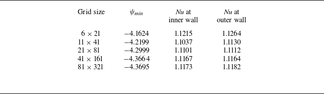


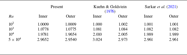


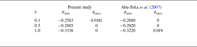


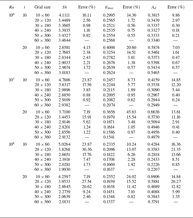


 Open access