


Non-technical Summary
The number of species identified in the fossil record within any given geological time period must partly be explained by both the total number of fossil specimens sampled from that interval and the geographic spread of those samples. The influence of numerical sampling intensity has been well studied, but the effects of geographic variance in sampling are comparatively unknown. To investigate this question, we repeatedly resample a dataset of modern global marine organisms (from the Ocean Biodiversity Information System) using spatial sampling parameters determined by the real geographic spread of fossil organisms as found in the Paleobiology Database. Our findings show that a significant proportion of the variance in fossil diversity through time can be attributed only to changes in the numbers and locations of fossils sampled. This is consistent with the claim that the spatial structure of the fossil record and how it is sampled largely determine the diversity history drawn from it and with the possibility that global diversity has been relatively constant over time.
Introduction
The incomplete and unevenly sampled nature of the fossil record was recognized as an obstacle to accurate reconstructions of trends in global Phanerozoic biodiversity as early as the mid-nineteenth century (Phillips Reference Phillips1860). Temporal unevenness in the numbers of recovered fossils (numerical sampling bias) inflates observed richness during time intervals from which more fossils have been reported. Traditionally employed by paleoecologists in small-scale regional studies, occurrence-based subsampling was adopted by the architects of the Paleobiology Database (PBDB) in an effort to recover a more accurate picture of changes in global richness over the Phanerozoic (Alroy et al. Reference Alroy, Marshall, Bambach, Bezusko, Foote, Fürsich, Hansen, Holland, Ivany, Jablonski, Jacobs, Jones, Kosnik, Lidgard, Low, Miller, Novack-Gottshall, Olszewski, Patzkowsky, Raup, Roy, Sepkoski, Sommers, Wagner and Webber2001, Reference Alroy, Aberhan, Bottjer, Foote, Fursich, Harries, Hendy, Holland, Ivany, Kiessling, Kosnik, Marshall, McGowan, Miller, Olszewski, Patzkowsky, Peters, Villier, Wagner, Bonuso, Borkow, Brenneis, Clapham, Fall, Ferguson, Hanson, Krug, Layou, Leckey, Nürnberg, Powers, Sessa, Simpson, Tomasovych and Visaggi2008). While the details differ across approaches (Alroy et al. Reference Alroy, Marshall, Bambach, Bezusko, Foote, Fürsich, Hansen, Holland, Ivany, Jablonski, Jacobs, Jones, Kosnik, Lidgard, Low, Miller, Novack-Gottshall, Olszewski, Patzkowsky, Raup, Roy, Sepkoski, Sommers, Wagner and Webber2001, Reference Alroy, Aberhan, Bottjer, Foote, Fursich, Harries, Hendy, Holland, Ivany, Kiessling, Kosnik, Marshall, McGowan, Miller, Olszewski, Patzkowsky, Peters, Villier, Wagner, Bonuso, Borkow, Brenneis, Clapham, Fall, Ferguson, Hanson, Krug, Layou, Leckey, Nürnberg, Powers, Sessa, Simpson, Tomasovych and Visaggi2008; Alroy Reference Alroy2010; Chao and Jost Reference Chao and Jost2012; Close et al. Reference Close, Evers, Alroy and Butler2018), subsampling yields increasingly accurate estimates of the temporal changes in both local and global biodiversity over the Phanerozoic.
Sampling bias, however, is not only numerical in origin—the spatial structure of fossil data may be critical as well (Close et al. Reference Close, Benson, Saupe, Clapham and Butler2020b; Antell et al. Reference Antell, Benson and Saupe2024; Fig. 1). Spatial biases in the way the fossil record is sampled differ fundamentally from numerical biases in that the geographic or environmental distribution of data is the primary concern. Biodiversity estimates today, as in the past, are directly influenced by the uneven distribution of taxa over the globe (Buffon Reference Buffon1774; von Humboldt and Bonpland Reference Humboldt and Bonpland1807). The nature of the geological record ensures that the sediments that might record this heterogeneity are neither deposited nor preserved with equal frequency over the Earth's surface. A first-order pattern in fossil diversity studies arises from the tendency of time intervals preserving more area and volume of sedimentary rock to yield more samples and hence more recovered taxa (Raup Reference Raup1976; Crampton et al. Reference Crampton, Beu, Cooper, Jones, Marshall and Maxwell2003; Smith and McGowan Reference Smith and Gowan2007; Ye and Peters Reference Ye and Peters2023). Fossil preservation is also nonrandom across paleoenvironments, and different environments are not consistently represented in the record (Schopf Reference Schopf1978; Peters Reference Peters2007; Patzkowsky and Holland Reference Patzkowsky and Holland2012; Shaw et al. Reference Shaw, Briggs and Hull2020). Furthermore, beyond the spatial inequities of sampling dictated by geological phenomena, a disproportionate percentage of fossil occurrences come from North America and Europe (Alroy et al. Reference Alroy, Marshall, Bambach, Bezusko, Foote, Fürsich, Hansen, Holland, Ivany, Jablonski, Jacobs, Jones, Kosnik, Lidgard, Low, Miller, Novack-Gottshall, Olszewski, Patzkowsky, Raup, Roy, Sepkoski, Sommers, Wagner and Webber2001; McGowan and Smith Reference McGowan and Smith2008; Ye and Peters Reference Ye and Peters2023) due largely to socioeconomic, political, and historical circumstances, with implications for the accuracy of biodiversity reconstructions (Raja et al. Reference Raja, Dunne, Matiwane, Khan, Nätscher, Ghilardi and Chattopadhyay2022).
Comparison of Paleobiology Database (PBDB) sampling in two distinct Paleozoic time bins, illustrating the wide variation in geographic sampling completeness within the PBDB. While it is true that the ca. 447 Ma time bin has more occurrences, those occurrences are also spread out across latitude and multiple ocean basins. On the other hand, the ca. 303 Ma time bin has occurrences concentrated in only one ocean basin and within a relatively small latitudinal band.

Previous studies have acknowledged and, in some cases, attempted to address variation in richness resulting from inconsistent spatial sampling by accounting for changes in outcrop area with time (Raup Reference Raup1976; Smith and Gowan Reference Smith and Gowan2007; Wall et al. Reference Wall, Ivany and Wilkinson2009). While this relates to the broader issue of spatial sampling bias, outcrop area alone is a poor proxy for spatial variation in sampling, because spatial biases originate from both the quantity and the spatial distribution of data. More recently, Close et al. (Reference Close, Benson, Alroy, Carrano, Cleary, Dunne, Mannion, Uhen and Butler2020a,Reference Close, Benson, Saupe, Clapham and Butlerb) used minimum spanning trees (MST) to approximate the spatial coverage of fossil occurrence data and found a strong correlation with numerical sampling-standardized diversity estimates. Reconstruction of biogeographic patterns even as fundamental as the latitudinal diversity gradient (LDG) can thus be complicated by changes in the spatial extent of fossil sampling (Jones et al. Reference Jones, Dean, Mannion, Farnsworth and Allison2021; Antell et al. Reference Antell, Benson and Saupe2024).
Here, we assess the impact of spatial sampling biases on our ability to reconstruct changes in global marine fossil richness over the Phanerozoic in a different way. Instead of subsampling fossil-record data from the PBDB through time, we repeatedly resample the same single dataset, in this case, modern marine skeletonized invertebrate biodiversity retrieved from the Ocean Biodiversity Information System (OBIS), using spatial sampling parameters defined by occurrences in the PBDB from different time intervals through the Phanerozoic. By holding real global richness static and subsampling that same dataset in different spatially explicit ways, we create a model for the Phanerozoic wherein all changes in recovered biodiversity are due only to changes in the spatial distribution of available occurrences through time. Comparing this purely spatially driven model with recovered fossil diversity over the Phanerozoic reveals the extent to which estimated changes in fossil biodiversity are driven by spatial sampling factors alone.
Methods
Datasets
Fossil data spanning the Phanerozoic were downloaded from the PBDB (here on 24 September 2021) and include global marine skeletonized macroinvertebrate occurrences belonging to six major phyla (Arthropoda, Brachiopoda, Cnidaria, Echinodermata, Mollusca, and Porifera), excluding occurrences with uncertain generic assignments and those with an age uncertainty greater than the longest Phanerozoic stage (~18 Myr). Primary references from which the data are drawn include Aberhan (Reference Aberhan1992), Cooper and Grant (Reference Cooper and Grant1977), Foster et al. (Reference Foster, Garvie, Weiss, Muscente, Aberhan, Counts and Martindale2020), Holland and Patzkowsky (Reference Holland and Patzkowsky2007), Fürsich (Reference Fürsich1999), Jung (Reference Jung1989), Manivit et al. (Reference Manivit, Le Nindre and Vaslet1990), Reboulet (Reference Reboulet1996), Reed (Reference Reed1944), and some 13,000 others. The PBDB dataset is analyzed and cleaned manually to remove nonmarine groups, out-of-date or poor taxonomy, and obvious errors. The final dataset contains 23,656 genera spread across 48 subequal ~11 Myr time bins that do not cross stage boundaries (following Alroy et al. Reference Alroy, Aberhan, Bottjer, Foote, Fursich, Harries, Hendy, Holland, Ivany, Kiessling, Kosnik, Marshall, McGowan, Miller, Olszewski, Patzkowsky, Peters, Villier, Wagner, Bonuso, Borkow, Brenneis, Clapham, Fall, Ferguson, Hanson, Krug, Layou, Leckey, Nürnberg, Powers, Sessa, Simpson, Tomasovych and Visaggi2008). Each time bin contains between 3259 and 46,310 occurrences and 353 and 2882 genera. The full dataset contains 590,144 occurrences.
Data on modern marine biodiversity are drawn from the OBIS (here on 26 September 2022) using the robis package (Provoost et al. Reference Provoost, Bosch and Appeltans2022). The database is searched for generic occurrences belonging to all extant taxonomic orders appearing in the PBDB dataset defined previously. Any OBIS occurrences marked as fossil are removed. The OBIS dataset is transformed into a geographic shapefile (Pebesma et al. Reference Pebesma, Bivand, Racine, Sumner, Cook, Keitt and Lovelace2018) and clipped to exclusively shallow-marine environments based on modern continental shelf geometries. Decapods are removed because they comprise an artificially high proportion of the modern diversity dataset. Finally, after OBIS occurrences have been grouped into equal-area grid cells (see below), cells with fewer than 1000 occurrences are removed, as these cells often represent aberrations in the dataset (e.g., latitude and longitude entered in reverse order) or contain very little shallow area (e.g., cells that mostly contain the deep ocean but may intersect a small part of the continental margins). The final OBIS dataset contains 3336 genera across 47 extant orders, for a total of 3,438,977 occurrences.
Quantification of Fossil Spatial Sampling through Time
To describe the geographic distribution of sampling in the PBDB and OBIS datasets, occurrences in both are first geographically binned into 812 equal-area grid cells covering the Earth surface using the R package dggridR (Barnes and Sahr Reference Barnes and Sahr2017). Each grid cell has an area of approximately 630,000 km2, and the mean distance between cell centroids is 855 km. The number of grid cells containing fossil data are counted for each of 48 time bins, and cells are grouped into five latitudinal bands (90–51°S, 50–23.4°S, 23.4°S–23.4°N, 23.4–50°N, and 51–90°N). Counts of cells and their geographic positions form the basis for the selection of modern OBIS cells for resampling. Fossil occurrence and cell MST distances are also calculated using the igraph (Csardi and Nepusz Reference Csardi and Nepusz2006) and sf (Pebesma et al. Reference Pebesma, Bivand, Racine, Sumner, Cook, Keitt and Lovelace2018) R packages. PBDB dataset variables, including the number of occurrences, percent shallow and percent tropical occurrences, and number of publications, are also recorded for each time bin.
Resampling the OBIS Dataset
First, a smaller subset (20%) of the OBIS dataset is randomly selected. This is done to increase processing speed and allow for the quantification of error based on random resampling. Modern cells containing OBIS data are selected to best match the latitudinal and longitudinal distributions of PBDB-occupied cells for each Phanerozoic time bin. To do this, modern cells are first assigned to the appropriate latitudinal band and then shifted eastward until the longitudinal distribution of modern cells within a latitudinal band completely covers the longitudinal distribution of PBDB cells in a given time bin (Fig. 2). For example, if paleo-occurrences in a time bin occupy three cells in the high north latitudinal bin, a set of equivalent OBIS cells will either be selected at those same longitude coordinates (if they contain data) or shifted together until cells can be sampled from those coordinates. In this way, the resampling procedure preserves absolute latitude (important for constraining the LDG) and captures the longitudinal spread of samples (which positively correlates with diversity at a given latitude today; Rosenzweig Reference Rosenzweig1995; Dallas et al. Reference Dallas, Holian and Caten2024; He et al. Reference He, Qin and Soininen2024). Given that there are many more modern cells containing data than there are paleo-cells in any time bin, longitudinal shifting is usually minimal and is most prevalent in the earliest stages of the Phanerozoic. There are always enough modern cells to cover the paleo-distribution with error less than ±25° of longitude.
Schematic showing an overview of the geographic subsampling process, which imposes the sampling “design” the fossil record has “given” us from each of 48 ~11 Ma time bins onto the Ocean Biodiversity Information System (OBIS) dataset of modern marine diversity for the same major groups on continental shelves. A, Geography and sampling intensity of a given latitudinal band from the Paleobiology Database (PBDB), with the pooled number of genera (top number) and occurrences (bottom number) within occupied equal-area cells. B, Geography of available modern data in the same latitudinal band, which are shifted together to the east (with potential wraparound) until their east–west distribution roughly matches the longitudinal distributions of PBDB occurrence data. C, Probability of sampling from each cell within a geographic cluster (e.g., if there are five bins that approximately match the position of the PBDB data, each of those has a probability of 0.2 of being sampled in a given run). D, Modern OBIS cells with approximately correct geography are subsampled so as to match the sampling intensity (no. of occurrences) of corresponding cells in the PBDB dataset, and the resulting number of genera is recorded for each. This process is repeated 25 times using a different random subsample of OBIS each time. See the text for more details.

After a suite of potential representative modern cells are selected, a subset is randomly chosen such that the number of modern cells is equivalent to the number of paleo-cells within a given latitudinal band and their longitudinal distributions match. After the cells have been selected, every OBIS occurrence from those cells is grouped into a dataset, and the number of unique genera is counted. In this way, the resampling protocol assumes complete sampling (or at least as complete as the OBIS dataset) of every PBDB-defined cell that contains data, which is an unrealistically optimistic scenario for fossil sampling but a worst-case scenario for our spatial model. To quantify error, the resampling process is run with a different random subset of the OBIS dataset 25 times.
Resampled OBIS diversity metrics are then compared with the actual fossil record of diversity, both raw (sampled in bin [SIB]) and sampling standardized (shareholder quorum subsampling [SQS]; Alroy Reference Alroy2010) as computed from the fossil data with the R package divDyn (Kocsis et al. Reference Kocsis, Reddin, Alroy and Kiessling2019), using linear regression analysis. Fossil diversity is also compared using linear regression to a variety of metrics computed from the PBDB dataset that broadly fall into three categories: sampling intensity factors (number of occurrences, number of publications, percentage of occurrences composed of any aragonite), spatial factors (number of cells, summed MST distance, latitudinal range of occurrences), and environmental factors (percentage of occurrences from tropical, reefal, shallow, and carbonate environments). Models are created using each PBDB metric alone, in combination with each other, and in combination with the OBIS resampled diversity estimate. Bin-to-bin first differences are also calculated for all diversity and additional dataset variables, and these are similarly subjected to linear regression analysis. Adjusted R 2 (adj. R 2) is calculated with the R statistical programming language and differs from R 2 in that the number of independent regressors (i.e., the number of independent variables) is considered in the calculation. It always produces a value less than or equal to R 2, and the explicit consideration of the number of variables being fit to a model helps reduce the effects of overfitting. Akaike information criterion (AIC) (Bozdogan Reference Bozdogan1987) model ranking scores are additionally used to compare the relative quality of statistical models—lower numbers represent higher quality, and an absolute difference between two represents a statistically significant difference in quality. AIC scores estimate model quality in a relative manner, so the values themselves are only relevant for models derived from the same dataset.
Results
Spatial Sampling in the Fossil and Modern Datasets
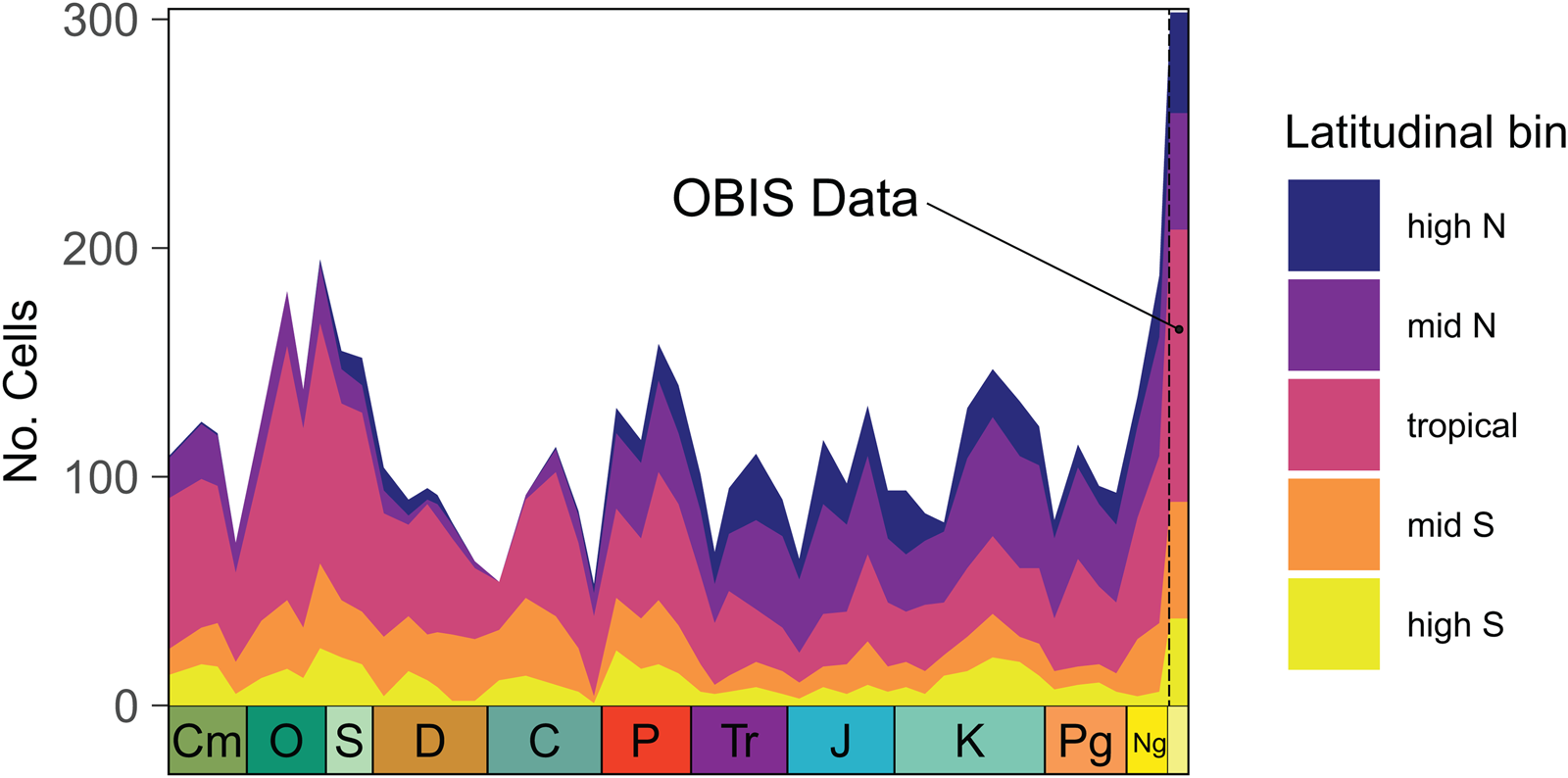
The number of equal-area grid cells occupied by marine-shelf fossil data per time interval varies from 53 to 195 (out of 812 total over the globe) but shows no trend through time (adj. R 2 = −0.019, p = 0.730; Fig. 3). As is true of occurrences (Alroy Reference Alroy2010), the latitudinal distribution of occupied cells is weighted toward the tropics in Paleozoic time bins and the northern midlatitudes during the Meso-Cenozoic. In comparison to the fossil record, modern marine shelves are both more completely and more evenly sampled, with 303 cells sampled and a latitudinal distribution of occupied cells that closely approximates that of all cells available to sample.
Spatial sampling through the Phanerozoic compared with modern data. The number of equal-area grid cells sampled across time within the coarse latitudinal bins used in this study, with cells sampled in the Ocean Biodiversity Information System (OBIS) dataset shown at the farthest right. Spatial sampling through time does not show a linear increase or decrease, but latitudinal sampling shifts northward, tracking the location of North America and Europe over the Phanerozoic; OBIS latitudinal sampling is more complete for every latitudinal band than every Paleobiology Database (PBDB) time bin. CM, Cambrian; O, Ordovician; S, Silurian; D, Devonian; C, Carboniferous; P, Permian; Tr, Triassic; J, Jurassic; K, Cretaceous; Pg, Paleogene; Ng, Neogene.
Resampled Modern Biodiversity versus PBDB Richness Estimates
Spatially resampled modern diversity varies across simulated time bins, with the greatest peaks in the Late Ordovician, middle Permian, and late Cenozoic (Fig. 4). All measures of genus richness are log transformed to reduce the influence of artificially high outliers, for example, the last Cenozoic time bin. Table 1 shows the results of linear correlations between resampled OBIS diversity, recovered fossil diversity, and the additional sample descriptors derived from the PBDB dataset. Without any additional adjustments, spatially resampled modern diversity correlates significantly with fossil diversity derived from both raw uncorrected, SIB diversity (R 2 = 0.408, p < 0.001) and sampling-standardized diversity estimates from SQS (Alroy Reference Alroy2010) (R 2 = 0.247, p < 0.001) (Table 1). Furthermore, the first differences in resampled modern diversity correlate with the first differences in raw and standardized fossil diversity (R 2 = 0.305, p < 0.001 for SIB, R 2 = 0.184, p = 0.001 for SQS) (Fig. 4B,C). As anticipated, bin-to-bin change in the number of fossil occurrences correlates strongly with SIB fossil diversity (R 2 = 0.642, p < 0.001 for value, R 2 = 0.647, p < 0.001 for first differences), but the correlation of occurrences with SQS diversity and first differences is low (R 2 = 0.183, p = 0.001) and nonexistent (R 2 = 0.018, p = 0.180), respectively, indicating that SQS standardization effectively removes the influence of variation in the number of samples. All SQS simulations were performed with a quorum value of 0.4.
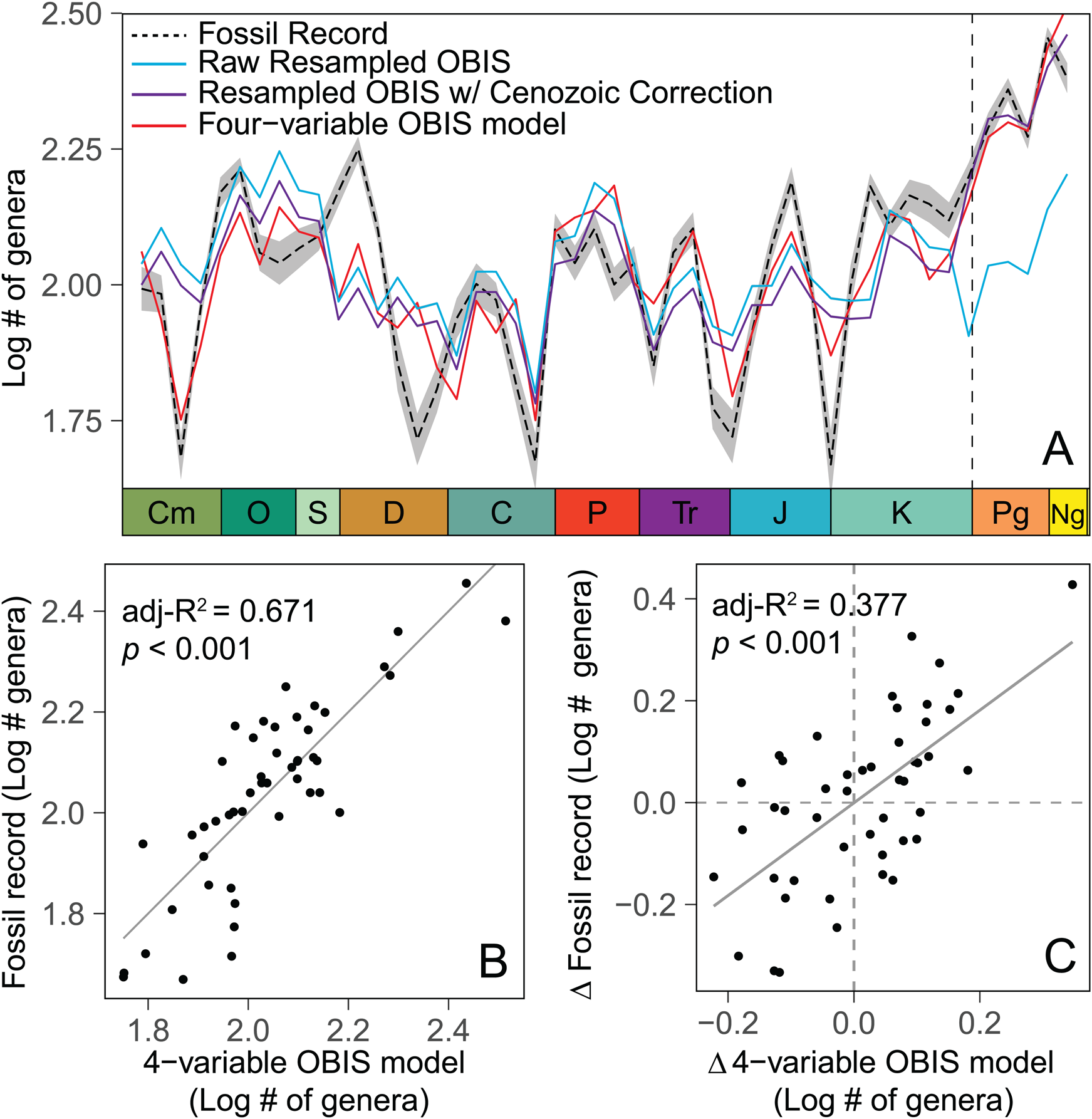
Comparison between three iterations of the resampled modern Ocean Biodiversity Information System (OBIS) model, which estimates expected fossil diversity based on only the spatial distribution of fossil data, and sampling-standardized shareholder quorum subsampling (SQS) richness of fossil marine invertebrate genera drawn from the Paleobiology Database (PBDB) (dashed black line). The raw OBIS model (blue), based only on resampled OBIS data, is adjusted to reflect the step increase into the Cenozoic (purple). The four-variable OBIS model (in red) further incorporates two additional variables: percent of shallow occurrences and latitudinal range of occurrences. A, Secular trends in both resampled model and SQS diversity estimates, with two-sigma error envelopes derived from replicate resampling. B, Correlation between the values of the four-variable OBIS model (best fit of all OBIS models based on adj. R 2 and Akaike information criterion [AIC] values) and fossil SQS. C, Correlation between the time bin to time bin first differences of those estimates, showing that the model generally predicts the magnitude and direction of change in fossil SQS diversity through time. The model explains about 67% of variance in the value of fossil SQS and 38% of the variance in bin-to-bin change. CM, Cambrian; O, Ordovician; S, Silurian; D, Devonian; C, Carboniferous; P, Permian; Tr, Triassic; J, Jurassic; K, Cretaceous; Pg, Paleogene; Ng, Neogene.
Results of linear correlations between resampled Ocean Biodiversity Information System (OBIS) diversity, recovered fossil diversity, and the additional sample descriptors derived from the Paleobiology Database (PBDB) dataset. AIC, Akaike information criterion. Bold indicates significance at the 0.05 level.

Comparison with a Spatially Randomized Dataset
By randomizing the taxonomic column in the OBIS dataset, we can create a modern biodiversity dataset that has no relevant spatial relationships (a taxon is equally likely to appear anywhere, with probability dependent only upon its number of occurrences), and this dataset can be used to test the importance of geography in our model results. While the spatially randomized dataset is still a significant predictor of the SQS value (R 2 = 0.204, p = 0.001), the correlation between first differences is eliminated (R 2 = 0.023, p = 0.156) (Table 1). A similar pattern holds when only brachiopods are analyzed; the spatial model is highly predictive of brachiopod-only SQS value (R 2 = 0.390, p > 0.001), but there is no significant relationship with first differences (R 2 = 0.054, p = 0.062).
Model Residuals
Spatially resampled model residuals were compared against PBDB dataset variables with potential explanatory power for Phanerozoic diversity; these include measures of sampling intensity (number of occurrences, publications), geography (latitudinal range of occurrences, number of equal-area cells sampled), and paleoenvironment (percentage of shallow or tropical occurrences), as well as temporal variables. Model residuals correlate with age in that the model substantially underestimates Cenozoic diversity. A model with a stepwise increase in diversity at the start of the Cenozoic improves the correlation and is clearly favored over one with a continuous increase in diversity through the Phanerozoic (adj. R 2 = 0.528 vs. 0.428, respectively; Table 1). When the Cenozoic age factor is included in the model, the correlation between resampled modern diversity and fossil SQS diversity increases substantially for value but changes little for first differences. After incorporation of the stepwise temporal variable, the remaining substantial offsets between the resampled modern diversity model and fossil SQS diversity can be accounted for with only two additional PBDB dataset parameters—percentage of shallow occurrences and absolute latitudinal range of occurrences (i.e., the highest latitude minus the lowest latitude, 0 to 180). The inclusion of these additional explanatory variables produces a model with four independent variables (resampled modern diversity estimate, stepwise time, percentage of shallow occurrences, and latitudinal range) and is referred to henceforth as the “four-variable model” (Fig. 4; Table 1). This model offers a large improvement in predictive power for the value of fossil SQS (R 2 = 0.671, p < 0.001) and a relatively smaller improvement in the correlation with SQS first differences (R 2 = 0.377, p < 0.001). Note that none of the temporal variation exhibited by the four-variable model comes from actual change in biodiversity with time, aside from the step increase at the Mesozoic/Cenozoic boundary.
Discussion
Our results indicate that the SQS-corrected view of skeletonized, marine invertebrate, fossil diversity can be reasonably reproduced with a simple null model of geographically resampled modern biodiversity, a binary age parameter, and two dataset variables relating to the geography and environment of sampling. Our null model can be generated without a single fossil taxon ever being named or described, and yet it approximates the very best estimates of both the overall trend of and bin-to-bin changes in Phanerozoic diversity inferred from the fossil record. These results question the validity of all reconstructions of biodiversity trends drawn from the fossil record, even after sampling standardization. Aside from the stepwise increase into the Cenozoic, they are also consistent with the hypothesis that the global number of skeletonized marine invertebrate genera is mostly static (Alroy et al. Reference Alroy, Marshall, Bambach, Bezusko, Foote, Fürsich, Hansen, Holland, Ivany, Jablonski, Jacobs, Jones, Kosnik, Lidgard, Low, Miller, Novack-Gottshall, Olszewski, Patzkowsky, Raup, Roy, Sepkoski, Sommers, Wagner and Webber2001), with apparent variation resulting almost entirely from changes in the spatial distribution of sampling.
The provocative nature of this statement demands rigorous interrogation of the analysis. Is it possible that our results could be determined solely by inadequacies in the OBIS dataset rather than real variation in the spatial coverage of fossil occurrence data? Do real diversity perturbations like mass extinctions stand out as outliers in the comparison between modeled and fossil record diversity, as they should so long as richness was suppressed for a substantial portion of a time bin? Finally, if our results are legitimate and truly indicate that recovered fossil biodiversity is driven by spatial sampling factors, what is the relative importance of numerical sampling intensity, spatial sampling intensity, and environmental factors?
Is OBIS Sufficient?
First, any attempt to describe modern biodiversity, including the OBIS database, is plagued by similar sampling biases, as in the fossil record (Hughes et al. Reference Hughes, Orr, Ma, Costello, Waller, Provoost, Yang, Zhu and Qiao2021). Inevitably, some regions will be undersampled (e.g., the Southern Ocean; Bonnet-Lebrun et al. Reference Bonnet-Lebrun, Sweetlove, Griffiths, Sumner, Provoost, Raymond, Ropert-Coudert and Van de Putte2023), some taxa will be underrepresented (e.g., bryozoans; Kopperud et al. Reference Kopperud, Lidgard and Liow2022), and some environments will be overrepresented (e.g., shallow coastal habitats; Klein et al. Reference Klein, Appeltans, Provoost, Saeedi, Benson, Bajona, Peralta and Bristol2019; Shaw et al. Reference Shaw, Briggs and Hull2020). Klein et al. (Reference Klein, Appeltans, Provoost, Saeedi, Benson, Bajona, Peralta and Bristol2019) note that half of described marine species are not found in OBIS (see also Webb and Vanhoorne Reference Webb and Vanhoorne2020), and those that are tend to be common and well known. However, a closer look at the OBIS dataset in comparison with PBDB data shows that our results are unlikely to arise from spatial or other biases within OBIS. For example, while more records come from Europe and North America in the OBIS, mirroring the socioeconomic and access issues seen in the PBDB (Fig. 5A), the bias is much less pervasive or impactful. Even where raw sampling numbers are relatively lower, biodiversity hotspots in places like the Indo-Pacific, Gulf of Mexico, and the African south coast still stand out within our subset of the OBIS dataset (Fig. 5B). By comparing data from the most recent PBDB time bin (the late Miocene–Quaternary) with the OBIS dataset, it becomes clear that OBIS is better sampled across latitude (Fig. 6) and taxonomy (Fig. 7). Southern Hemisphere sampling in the PBDB is comparatively incomplete, and latitudinal sampling deficiencies are only worse in deep time. The most recent PBDB time bin is also overwhelmingly dominated by mollusks, especially bivalves (69% and 41%, respectively), while the OBIS contains a taxonomically broader suite of organisms (only 37% mollusk and 18% bivalve; see also Webb and Vanhoorne Reference Webb and Vanhoorne2020). The median OBIS cell contains five of the six phyla examined in this study, while the median recent PBDB cell only contains two. Finally, comparing cells that are occupied by occurrences in both datasets shows that well-represented cells in the PBDB are typically well sampled in the OBIS, but the reverse is not true (Fig. 8). In sum, there are many more cells sampled in the OBIS and those cells are consistently better sampled than those of the PBDB. Even if sampling of the OBIS is not complete—biological sampling can never be considered 100% comprehensive—sampling within the OBIS is certainly comprehensive enough for comparisons to the PBDB and for global spatial diversity statistics.
Ocean Biodiversity Information System (OBIS) occurrences and richness in our subset of the data. A, OBIS occurrences within equal-area cells. B, OBIS generic richness within equal-area cells. Patterns in A are largely driven by spatial sampling biases (e.g., a greater number of scientific institutions in the Northern Hemisphere), but important marine invertebrate diversity hotspots can be seen in B, implying that imperfect spatial sampling has not greatly distorted spatial diversity patterns in the OBIS.

Latitudinal sampling in the Ocean Biodiversity Information System (OBIS) dataset (blue) versus the most recent (mid-Miocene to Recent) time bin of the Paleobiology Database (PBDB) (red). OBIS sampling is more complete in the Southern Hemisphere (A), but both exhibit the latitudinal diversity gradient (B).

The number of phyla per sampled cell in the Ocean Biodiversity Information System (OBIS) dataset (A) versus the most recent time bin of the Paleobiology Database (PBDB) (B).

The numbers of families present in cells occupied in both the Ocean Biodiversity Information System (OBIS) and most recent Paleobiology Database (PBDB) data. All diverse PBDB cells are also diverse in OBIS, but the reverse is not the case.

Second, our results cannot be dismissed as noise. If spatial sampling factors are important for driving the similarity between SQS diversity and resampled modern diversity, then removing the spatial component of the dataset through randomization should eliminate the correlation, and this is exactly what happens. When the taxonomic column of the OBIS dataset is randomized, effectively removing all relationships between space and the distribution of organisms on the Earth, the model fails to accurately predict bin-to-bin change in the SQS value of the fossil record (adj. R 2 = 0.023, p = 0.156; Table 1). Furthermore, all versions of the model, including the spatially randomized one, predict bin-to-bin change in SQS value better than does the number of fossil occurrences through time. If SQS reduced the influence of spatial sampling bias as much as it does numerical sampling bias, we would expect the correlation between SQS and the number of occurrences through time to be similar to the correlation between SQS and resampled modern diversity, and this is not the case (Table 1).
Finally, our model is methodologically complex but theoretically simple. From a theoretical standpoint, the model can be conceived as sampling the modern landscape of biodiversity with the same or similar spatial fidelity as that in the fossil record. If the spatial distribution of fossil sampling were sufficient, there should be no appreciable change in predicted richness, as the same data are being sampled each time. There is no particularly good reason to believe that marine biodiversity in deep time was spatially arrayed in a similar manner to modern biodiversity—in fact there are many reasons to believe this not to be the case. While some manifestation of the LDG seems to be more or less persistent, the shape of that relationship has varied significantly over time, from unimodal to bimodal to flat (Crame Reference Crame2001; Alroy et al. Reference Alroy, Aberhan, Bottjer, Foote, Fursich, Harries, Hendy, Holland, Ivany, Kiessling, Kosnik, Marshall, McGowan, Miller, Olszewski, Patzkowsky, Peters, Villier, Wagner, Bonuso, Borkow, Brenneis, Clapham, Fall, Ferguson, Hanson, Krug, Layou, Leckey, Nürnberg, Powers, Sessa, Simpson, Tomasovych and Visaggi2008; Mannion Reference Mannion2020), and the latitudinal and longitudinal distribution of taxa have clearly changed with the changing configuration of continents and ocean basins (Valentine Reference Valentine1973). Nevertheless, the modern landscape can suffice as a null hypothesis for our spatial sampling model, and if the spatial distribution of organisms on the Earth has changed dramatically through deep time, it should be relatively easy to reject our null hypothesis. Again this is not the case. Our results suggest that, when estimating trends or changes in global-scale diversity, even SQS-standardized fossil diversity remains substantially impacted by spatial sampling factors.
Insights from Model Residuals
If the resampled OBIS model can be considered a null model of expected SQS fossil diversity, a closer look at time bins when the raw model and subsequent adjustments perform poorly may be informative.
First, a fundamental question arising from paleobiodiversity studies is whether the dramatic apparent increase in biodiversity into the Cenozoic and toward the present is real or an artifact (Alroy et al. Reference Alroy, Marshall, Bambach, Bezusko, Foote, Fürsich, Hansen, Holland, Ivany, Jablonski, Jacobs, Jones, Kosnik, Lidgard, Low, Miller, Novack-Gottshall, Olszewski, Patzkowsky, Raup, Roy, Sepkoski, Sommers, Wagner and Webber2001). Consistent with Alroy (Reference Alroy2010), our analysis of SQS richness shows an approximately twofold increase in the average richness of Cenozoic time bins compared with those of the Paleo-Mesozoic, even when unconsolidated sediments are excluded from the analysis. To test the hypothesis of a step change in marine biodiversity following the Cretaceous–Paleogene mass extinction, we compare models that include no time-dependent variable, a “Cenozoic or not” factor, and time as a continuous variable (i.e., bin age in millions of years). Results (Table 1) clearly favor the “Cenozoic or not” model as the model with the most explanatory power for both SIB and SQS fossil diversity estimates, indicating the likelihood of a real stepwise increase in marine biodiversity starting near the Cretaceous/Paleogene boundary. However, geographic sampling proxies like the resampled OBIS diversity estimate and the summed MST length of PBDB-sampled cells accurately explain the observed increase in SQS and SIB richness during the Cenozoic, indicating little support for a continuous increase in richness among marine invertebrates over the last 66 Myr. Close and colleagues likewise found a stepwise increase in the biodiversity of marine animals (Close et al. Reference Close, Benson, Saupe, Clapham and Butler2020b) and terrestrial vertebrates (Close et al. Reference Close, Benson, Alroy, Carrano, Cleary, Dunne, Mannion, Uhen and Butler2020a) in the early Cenozoic that they could not attribute to a spatial sampling artifact. Whether this observed stepwise increase is real or the result of additional bias (e.g., more splitting of Cenozoic genera; Hendy Reference Hendy, Allison and Bottjer2010) remains an open question and deserves closer investigation.
After correcting for the step up into the Cenozoic, residuals correlate weakly but significantly with two variables drawn from the PBDB dataset (Fig. 4A). First, the percentage of fossil occurrences from relatively shallow environments (roughly, shallower than benthic assemblage zone 4, exclusive) correlates positively with the residuals (adj. R 2 = 0.193, p = 0.001). Residual correlation with an environmental variable is unsurprising, because the OBIS model does not take any paleoenvironmental information into account, and biological diversity certainly varies across environments. However, to the degree that times with proportionately more fossils from shallow environments also reflect times of greater continental flooding and expansion of shallow seas, this correlation could reflect a real signal of biotic response to expansion and contraction of habitat area (Peters and Husson Reference Peters and Husson2017). The extent of shallow-marine sediment is also seen to correlate positively with spatially subsampled diversity by Close et al. (Reference Close, Benson, Saupe, Clapham and Butler2020b), suggesting species–area effects (Rosenzweig Reference Rosenzweig1995) not predicted by sampling alone. The significant middle Cambrian overestimation of PBDB diversity, for example, disappears in the four-variable OBIS model that incorporates percent shallow occurrences (Figs. 4A, 9), perhaps reflecting a real increase in diversity during the expansion of shallow-water habitats associated with continental flooding during the Sauk sequence. Given the nature of Paleo-Mesozoic fossil data, a relative increase in the sampling of inferred deep occurrences (or a reduction in the proportion of shallow occurrences) might additionally reflect times of increased ocean anoxia. Deep environments are often inferred from the presence of black shales and dark-colored micrites, which are typically depauperate and more directly indicative of anoxia than they are of deep water (Smith et al. Reference Smith, Schieber and Wilson2019). Anoxia might therefore contribute to the forces producing relatively lower than expected fossil SQS diversity (e.g., Peters Reference Peters2007) in intervals with proportionally less shallow sampling.
Several other environmental variables were tested, including the percentage of tropical and reefal occurrences, both of which are often associated with higher origination and standing diversity in the literature (Aberhan and Kiessling Reference Aberhan, Kiessling and Talent2012), but none explained any significant proportion of variation in the residuals. Rather than showing that these variables are not important for standing diversity, this indicates that modern and paleoenvironmental trends diverge in this respect—in the modern dataset, the tropics and reefal locations have not changed from where they were in the past, but the location of the shallow ocean certainly has. In other words, the modern dataset already has a spatial concentration of diversity at the tropics (and at reefs, which are mostly tropical), so no additional information from the fossil dataset is necessary to explain these spatial patterns. The only other variable to significantly correlate with model residuals was a simple measure of the absolute latitudinal range of fossil occurrences in each time bin (adj. R 2 = 0.098, p = 0.017), an unsurprisingly weak correlation, given that the model already attempts to account for latitudinal variation in sampling. Its incorporation as an additional explanatory variable implies that the original OBIS model may have treated latitude with too little granularity.
The OBIS Cenozoic-corrected and four-variable models tend to overestimate richness in time bins at or immediately after the major mass extinctions (Fig. 4A), but model residuals for most of these time bins (Fig. 9) do not stand out, reinforcing that rebound from extinctions largely happens within the succeeding time bin at this scale, as suggested by other studies of regional and global biodiversity (Alroy et al. Reference Alroy, Aberhan, Bottjer, Foote, Fursich, Harries, Hendy, Holland, Ivany, Kiessling, Kosnik, Marshall, McGowan, Miller, Olszewski, Patzkowsky, Peters, Villier, Wagner, Bonuso, Borkow, Brenneis, Clapham, Fall, Ferguson, Hanson, Krug, Layou, Leckey, Nürnberg, Powers, Sessa, Simpson, Tomasovych and Visaggi2008; Close et al. Reference Close, Benson, Saupe, Clapham and Butler2020b). The Late Devonian biodiversity crisis is an exception, perhaps owing to its duration over a longer interval of time. PBDB richness is much lower compared with the OBIS model predictions at the Jurassic/Cretaceous (J/K) boundary (Fig. 4A). The latter is especially interesting given that the J/K boundary is generally poorly understood and may be an interval especially affected by sampling biases (Tennant et al. Reference Tennant, Mannion and Upchurch2016). On the other hand, the interval from the end-Silurian to the Middle Devonian stands out as a period with uncharacteristically high residuals—that is, fossil diversity is higher than expected by the OBIS model. Close et al. (Reference Close, Benson, Saupe, Clapham and Butler2020b) also find SQS diversity to be elevated at this time relative to their spatially standardized analysis. One might infer this to reflect an expansion in marine biodiversity (Klug et al. Reference Klug, Kröger, Kiessling, Mullins, Servais, Frýda, Korn and Turner2010; Ruban Reference Ruban2013), yet the interval encompassing the well-known Ordovician radiation does not stand out as a time of elevated richness compared with model estimates. The Early–Middle Devonian, however, is a particularly spatially well-sampled interval, specifically with an atypically high latitudinal range of sampling, even though the number of occurrences collected from that interval is unremarkable.
Residuals between the resampled four-variable Ocean Biodiversity Information System (OBIS) model and fossil shareholder quorum subsampling (SQS) diversity. Dashed lines show the ages of the “big five” mass extinctions. CM, Cambrian; O, Ordovician; S, Silurian; D, Devonian; C, Carboniferous; P, Permian; Tr, Triassic; J, Jurassic; K, Cretaceous; Pg, Paleogene; Ng, Neogene.

Moving Forward
What can be done to remedy or address the effects of spatial bias in the fossil record? One line of thought is to simply increase sampling efforts in previously undersampled locations, including across the Global South. Given that the density of sampling is much higher in North America and Europe than in the rest of the world (Ye and Peters Reference Ye and Peters2023), much could be learned from this process, and many gaps in knowledge might be filled. However, it is likely that biases originating from the spatially nonrandom distribution of exposed sedimentary rock of appropriate age (rather than from sociopolitical phenomena) would still influence interpretations of the fossil record, even after substantial sampling efforts, because the samples necessary to fill the gaps simply do not exist. Another approach is to focus on numerically standardized paleobiological diversity within multiple areas of comparable spatial extent drawn from each time interval (Close et al. Reference Close, Benson, Alroy, Carrano, Cleary, Dunne, Mannion, Uhen and Butler2020a,Reference Close, Benson, Saupe, Clapham and Butlerb), allowing for direct comparisons across geological time at spatially consistent scales. While both increased sampling and improved understanding of diversity variance within and across equal spatial regions are important for addressing the spatial structure inherent in the fossil record, spatially informed quantitative and statistical methods are critical as well. Paleobiologists will benefit from new focus on the development of novel spatial resampling techniques (e.g., recent work by Antell et al. [Reference Antell, Benson and Saupe2024]) and from interdisciplinary studies with ecologists and neontologists experienced in dealing with spatial sampling questions.
Additionally, future efforts to address spatial bias in the sampling-standardized record of fossil diversity should focus on differentiating the real biogeographic effects imposed by plate tectonics, continental flooding, and global climate change from the artificial variation introduced by the distribution of sampling. The spatial distribution of marine taxa today is not likely to approximate that in, for example, the Middle Devonian, because in the latter, the Northern Hemisphere was mostly devoid of land or shallow water (Scotese Reference Scotese2016) and the continents were less dispersed than today (Zaffos et al. Reference Zaffos, Finnegan and Peters2017). Likewise for the Cretaceous hothouse, with much warmer temperatures and no ice at the poles. As well, given the preponderance of data from North America and Europe and their northward shift out of the tropics over the last ~200 Myr, if anything like the modern LDG is typical of the Phanerozoic, numerically standardized estimates alone are still likely to underestimate mid–late Mesozoic diversity in comparison to the Paleozoic. To what degree are recovered patterns in paleobiodiversity in space and time real and due to such factors, as opposed to driven purely by spatial (and numerical) sampling limitations?
In conclusion, we show that a subset of the OBIS dataset of modern global biodiversity with taxonomic membership comparable to the skeletonized marine invertebrate fossil record, when sampled spatially as dictated by the fossil record, produces predicted richness values and first differences that reasonably correlate with fossil richness estimates, even after state-of-the-art numerical subsampling procedures have been applied. As also deduced by Close et al. (Reference Close, Benson, Saupe, Clapham and Butler2020b) using entirely different methods, these results strongly caution the overinterpretation of biodiversity trends inferred from the fossil record and are consistent with the argument that global marine biodiversity has been largely static over the Phanerozoic, with apparent variation resulting almost entirely from changes in the spatial distribution of sampling. Changes in spatial sampling parameters, like the number and distribution of geographic cells sampled, their summed MST distances, and their latitudinal range, are at least as important for predicting fossil richness values as factors associated with numerical sampling intensity. This analysis highlights the importance of the spatial distribution of sampling in analyses of large-scale fossil biodiversity and echo the call from Antell et al. (Reference Antell, Benson and Saupe2024) for the development of new methodologies that explicitly account for spatial biases in the fossil record.
Acknowledgments
We thank all of the original authors, data enterers, programmers, and contributors whose work produced the Paleobiology Database and the Ocean Biodiversity Information System. Without you, these kinds of analyses would not be possible. M. Clapham and an anonymous reviewer provided valuable feedback that helped refine the article, and we are grateful to them. Special thanks to J. Kastigar in the editorial office for patience and understanding. DBP was supported by Collaboration for Unprecedented Success and Excellence (CUSE) grant II-38-2020 from Syracuse University's Office of Research to LCI and fellowships from the Department of Earth Sciences and the Graduate School. This paper is Publication No. 493 for the Paleobiology Database.
Competing Interests
The authors declare no competing interests.
Data Availability Statement
Data and R code are available from the Dryad Digital Repository: https://doi.org/10.5061/dryad.2280gb621.


 Open access