2. Geometric tools

In the section, we introduce some terminology, and prove some lemmas used in the proofs of Theorems 1 and 2.

Let $0 < r \leq \pi/2$ denote the radius of spindle convexity. As r is fixed throughout the paper, we will generally omit it from the notation. By the distance of two points on $S^2$ , we will generally mean their spherical distance. The set $B\subset S^2$ is a spherical circular disc of radius r if it is the set of points that has distance at most r from a fixed point of $S^2$ , called the centre of the disc. The boundary of B is then the intersection of $S^2$ with a plane that has distance $\cos r$ from the origin, and is hence a Euclidean circle of radius $\sin r$ . If a set $K\subset S^2$ is spherically r-spindle convex – that is, it coincides with its spherical r-spindle convex hull – we will refer to it as a spherical r-convex disc or spherical spindle convex disc; we note that we emphasize the word circular in the previous definition to make the distinction between the two clear.

A subset D of a spherical spindle convex disc K is called a spherical disc-cap if $D = \operatorname{cl} (K\cap B^\mathrm{c})$ for some spherical circular disc B of radius r, where $\operatorname{cl}\!(\!\cdot\!)$ and $\cdot^\mathrm{c}$ denote the closure and complement of a set, respectively. We note that the disc-cap D is bounded by a segment of $\partial K$ , and a segment of $\partial B$ . As discussed above, while the latter is obtained from a spherical circular disc, it is also a Euclidean circular arc, which has (Euclidean) radius $\sin r$ , and some central angle measured in the plane in which the arc lies.

We use the usual o and O notation: $g=o(h)$ as $x\to x_0$ if $\lim_{x \to x_0} g(x)/h(x) = 0$ ; $g=O(h)$ if $ \limsup_{x\to x_0} g(x)/h(x) <\infty$ . We also write $g\sim h$ as $x\to x_0$ when $g=g(x)$ and $h=h(x)$ are asymptotically equal, i.e. $g(x)/h(x)\to 1$ as $x\to x_0$ .

We first collect some definitions and results from differential geometry.

To state the second lemma, regarding disc-caps of spindle convex sets, we recall the following. For a differentiable curve $\gamma\subset S^2$ , its normal plane at a point $x_0 \in \gamma$ is defined as the plane that contains $x_0$ and is perpendicular to the tangent vector of $\gamma$ at $x_0$ . Since we know that the vector pointing from the origin to $x_0$ is perpendicular to the tangent plane of the sphere at $x_0$ , it is also perpendicular to the tangent vector of $\gamma$ at $x_0$ . This implies that the normal plane contains the origin, and hence intersects the sphere in a great circle.

We refer to $x_0$ as the vertex, and to t as the height of the cap.

Lemma 3. Let K be a spherical r-convex disc with $C^5$ boundary and with the property that $\kappa_\mathrm{g}(x) > \cot r$ for every $x\in \partial K$ , and let $\varrho$ be an arc-length parametrisation of $\partial K$ . We denote by $A(t,s_0)$ the area of the spherical disc-cap with vertex $\varrho(s_0)$ and height t, and by $\Delta\theta(t,s_0)$ the central angle of the circular arc that determines this disc-cap. Then

$$ \Delta\theta(t,s_0) = \vartheta_1 t^{1/2} + \vartheta_2 t^{3/2} + O(t^2), \quad A(t,s_0) = v_1 t^{3/2} + v_2 t^{5/2} + O(t^{7/2}), $$

where the coefficients are dependent on s₀, namely

\begin{align*} \vartheta_1 & = \frac{2}{\sin r}\sqrt{\frac{2}{\Delta \kappa_\mathrm{g}}}, \qquad v_1 = \frac 43 \sqrt{\frac{2}{\Delta \kappa_\mathrm{g}}}, \\ \vartheta_2 & = \sqrt{\frac{2}{\Delta\kappa_\mathrm{g}}} \frac{-\frac12\Delta\kappa_\mathrm{g}^4-\frac32\cot r\cdot(\Delta\kappa_\mathrm{g})^3 - \frac56(1+\cot^2 r)(\Delta\kappa_\mathrm{g})^2-\frac16\kappa_\mathrm{g}''\Delta\kappa_\mathrm{g} + \frac{5}{18} (\kappa_\mathrm{g}')^2}{\sin r\cdot(\Delta\kappa_\mathrm{g})^3}, \\ v_2 & = \sqrt{\frac{2}{\Delta\kappa_\mathrm{g}}}\frac{-\frac15\Delta\kappa_\mathrm{g}^4 - \frac35\cot r\cdot(\Delta\kappa_\mathrm{g})^3-\frac35(1+\cot^2 r)(\Delta\kappa_\mathrm{g})^2 - \frac{1}{15}\kappa_\mathrm{g}''\Delta\kappa_\mathrm{g} + \frac19(\kappa_\mathrm{g}')^2} {(\Delta\kappa_\mathrm{g})^3}, \end{align*}

where $\Delta\kappa_\mathrm{g} = \Delta\kappa_\mathrm{g}(s_0) = \kappa_\mathrm{g}(s_0)-\cot r$ and $\kappa_\mathrm{g}'=\kappa_\mathrm{g}'(s_0)$ .

Proof. We may assume without loss of generality that $\varrho$ is a parametrisation with positive orientation, $s_0=0$ , $\varrho(0) = (0,0,1)$ , and $\dot{\varrho}(0)=(1,0,0)$ ; hence, $\varrho(0)\times \dot{\varrho}(0)=(0,1,0)$ . Using Lemma 1, we can express the higher derivatives of $\varrho(s)$ in terms of the orthonormal basis $\varrho(s)$ , $\dot{\varrho}(s)$ , and $\varrho(s)\times \dot{\varrho}(s)$ . By the smoothness condition on the boundary, this leads us to obtain the fourth-order series expression for $\varrho(s)$ around $\varrho(0)$ :

(2) \begin{align} \varrho(s) & = \bigg(s-\frac{s^3}{6}\big(\kappa_\mathrm{g}^2+1\big)-\frac{s^4}{8}\kappa_\mathrm{g}\kappa_\mathrm{g}' + O(s^5), \nonumber \\ & \qquad \frac{s^2}{2}\kappa_\mathrm{g}+\frac{s^3}{6}\kappa_\mathrm{g}' + \frac{s^4}{24}\big(\kappa_\mathrm{g}''-\kappa_\mathrm{g}-\kappa_\mathrm{g}^3\big) + O(s^5), \nonumber \\ & \qquad 1-\frac{s^2}{2} + \frac{s^4}{24}\big(\kappa_\mathrm{g}^2+1\big)+O(s^5)\bigg). \end{align}

Now, let $C=C(t)$ be the spherical circular disc that determines the spherical disc-cap with vertex $\varrho(0)$ and height t. Then, by Lemma 2, the centre of C is at distance $r+t$ from the origin along the great circle $S^2 \cap \{x=0\}$ , implying that C has centre $(0, \sin(r+t), \cos(r+t))$ . This vector forms an orthonormal basis together with the vectors (1, 0, 0) and $(0, -\cos(r+t), \sin(r+t))$ , thus $\partial C$ can be parametrised as

(3) \begin{align} & \big(\sin r\cos\varphi, \nonumber \\ & \phantom{\big(} \cos r\sin(r+t) + \sin r\cos(r+t)\sin\varphi, \nonumber \\ & \phantom{\big(} \cos r\cos(r+t) - \sin r\sin(r+t)\sin\varphi\big), \quad \varphi \in [0,2\pi ], \end{align}

since the Euclidean radius of $\partial C$ is $\sin r$ , and its centre has distance $\cos r$ from the origin. Note that the closest point of $\partial C$ to $\varrho(0)$ is at the parameter value $\varphi=3\pi/2$ ; hence, for small enough t, the arc of $\partial C$ that is contained in K is given by parameter values in $[\pi, 2\pi]$ .

Our first goal is to express the intersection points of $\partial K$ and $\partial C$ in terms of t. Let $x_-$ and $x_+$ denote the x-coordinates of the points of intersection.

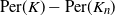
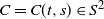
Consider the orthogonal projection of the construction to the tangent plane $z=1$ to the sphere at $\varrho(0)$ , or equivalently, the xy plane, see Figure 1. The projection of $\partial K$ is the graph of the function

$$ K(x) \, :\!= \, \frac{x^2}{2}\kappa_\mathrm{g} + \frac{x^3}{6}\kappa_\mathrm{g}' + \frac{x^4}{24}\big(\kappa_\mathrm{g}'' + 3\kappa_\mathrm{g} + 3\kappa_\mathrm{g}^3\big) + f(x) $$

in the xy plane near the origin, where $f(x) = O(x^5)$ as $x\to 0$ . This can be obtained from the series expansion (2) of $\varrho(s)$ as follows. Let x denote the first coordinate of the parametrisation. Then the powers of x, and thus any polynomial expression of x, can be expressed in terms of s (up to some $O(s^m)$ term), and matching the coefficients to the second coordinate of the expansion yields the expression for K(x). The necessary arc of the projection of $\partial C$ is described for $x\leq \sin r$ by the function

$$C(x) \, :\!= \, \cos r \sin(r+t)-\cos(r+t)\sqrt{\sin^2 r-x^2}$$

for arbitrary t when $r=\pi/2$ , and for $t<\pi/2-r$ when $r<\pi/2$ . This can be assumed since we are interested in the behaviour as $t\to 0$ .

Figure 1. Projection of a disc-cap to the tangent plane.

The equality $K(x) = C(x)$ gives us an implicit relationship between t and x at the points of intersection. We use implicit differentiation (see [Reference Koepf12]) to derive the fourth-order Taylor expansion of t around 0. This can be done as follows. Introduce the notation $F(x,t)\, :\!= \,K(x)-C(x)$ ,

$$F_1(x,t) \, :\!= \, -\frac{\partial F(x,t)/\partial x}{\partial F(x,t)/\partial t},$$

and, recursively,

$$F_k(x,t)\, :\!= \,\frac{\partial F_{k-1}(x,t)}{\partial x} + \frac{\partial F_{k-1} (x,t)}{\partial t} \cdot F_1(x,t)$$

for $k\geq 2$ . Then, applying the two-dimensional chain rule to F(x,t(x)), where we now consider $t=t(x)$ as a function of x, we have $t'(x) \, :\!= \, {\mathrm{d}t(x)}/{\mathrm{d}x} = F_1(x,t(x))$ ; further, by differentiating $F_{k-1}(x,t(x))$ , we obtain

$$F_k(x,t(x)) = \frac{\partial F_{k-1}(x,t(x))}{\partial x}.$$

Thus, the kth derivative of $t=t(x)$ (with respect to x) coincides with $F_k(x,t(x))$ . This gives us a method to derive the fourth-order Taylor expansion of t around 0. Since F is polynomial in x and trigonometric in t, this is a lengthy but straightforward computation. As such, we chose not to include the steps here explicitly; however, to ensure the correctness of the calculations, and make the subsequent formula verifiable, we refer to the supplementary computational script [Reference Nagy and Vígh15]. Applying this method yields that at the points of intersection,

$$ t=\frac{x^2}{2}(\kappa_\mathrm{g}-\cot r) + \frac{x^3}{6}\kappa_\mathrm{g}' + \frac{x^4}{24}\big(\kappa_\mathrm{g}'' + 3\kappa_\mathrm{g}^3 + 9\kappa_\mathrm{g} -3\cot^3 r - 9\cot r\big) + O(x^5) $$

as $x\to 0$ . Note that since $\partial K$ is of class $C^5$ , the function K(x), and consequently the remainder term f(x), is four times differentiable. If a function is $O(x^n)$ and is differentiable at 0, its derivative is $O(x^{n-1})$ around zero, which in our case implies that the first four derivatives of f(x) equal 0 at $x=0$ . Since the implicit differentiation used above requires at most the fourth derivative of K(x) at point $x=0$ , the term f(x) does not affect the results.

By introducing the notation $\Delta\kappa_\mathrm{g} = \kappa_\mathrm{g} - \cot r$ , the above formula can be reformulated as

$$ t=\frac{x^2}{2}\Delta\kappa_\mathrm{g} + \frac{x^3}{6}\kappa_\mathrm{g}' + \frac{x^4}{24}(\kappa_\mathrm{g}'' + 3(\Delta\kappa_\mathrm{g})^3 + 9\cot r(\Delta\kappa_\mathrm{g})^2 + 9(1+\cot^2r)\Delta\kappa_\mathrm{g}) + O(x^5). $$

We aim now to obtain x as a function of t. There are two solutions around $x=0$ , $x_-<0<x_+$ , obtained by inverting the function on the negative and positive domains, respectively. To do this, we use [Reference Fodor and Montenegro Pinzón8, Lemma 2] (see also [Reference Gruber11, Lemma 2] in a more general form). By the assumptions, $\Delta\kappa_\mathrm{g} >0$ , hence the function t(x) is strictly increasing in a small enough neighbourhood $(0,\varepsilon)$ , and the above lemma can be used. The inverse on the negative domain can be obtained by inverting the function $t(-x)$ on $x>0$ , which by the same argument is strictly increasing in an appropriate interval there, and taking its negative. With this approach, we get

$$ x_+ = C_1t^{1/2} + C_2t + C_3t^{3/2} + O(t^2), \qquad x_- = -C_1t^{1/2} + C_2t - C_3t^{3/2} + O(t^2), $$

where

\begin{align*} C_1 & = \sqrt{\frac{2}{\Delta}\kappa_\mathrm{g}}, \qquad C_2 = \frac{-\kappa_{\mathrm{g}}{\prime}}{3(\Delta\kappa_{\mathrm{g}})^2}, \\ C_3 & = \sqrt{\frac{2}{\Delta}\kappa_\mathrm{g}} \frac{-\frac{1}{4}\Delta\kappa_{\mathrm{g}}^4-\frac{3}{4}\cot r\cdot(\Delta\kappa_\mathrm{g})^3 - \frac34(1+\cot^2 r)(\Delta\kappa_\mathrm{g})^2-\frac{1}{12}\kappa_\mathrm{g}''\Delta\kappa_\mathrm{g} + \frac{5}{36}(\kappa_\mathrm{g}')^2}{(\Delta\kappa_\mathrm{g})^3}. \end{align*}

Now, since the intersection points lie on $\partial C$ , by (3) we have $\sin r \cos \theta_+ = x_+$ for some parameter value $\theta_+\in[0,2\pi]$ . As noted before, we know that the segment of $\partial C$ contained in K is obtained for parameter values in $[\pi,2\pi]$ for small enough t. Hence, we obtain

\begin{align*} \theta_+ = \frac{3\pi}{2} + \arccos\bigg(\frac{x_+}{\sin r}\bigg) & = \frac{3\pi}{2} + \frac{x_+}{\sin r} + \frac{x_+^3}{6\sin^3r} + O(x_+^5) \\ & = \frac{3\pi}{2} + \frac{C_1}{\sin r}t^{1/2} + \frac{C_2}{\sin r}t + \bigg(\frac{C_3}{\sin r} + \frac{C_1^3}{6\sin^3 r}\bigg)t^{3/2} + O(t^2), \end{align*}

where we used the expansion of the function $\arccos(x)$ around $x=0$ . Using a similar argument for the solution to $\sin r\cos\theta_- = x_-$ , we obtain

$$ \Delta\theta \, :\!= \, \theta_+ - \theta_- = \frac{2C_1}{\sin r}t^{1/2} + \frac{2}{\sin r}\bigg(C_3+ \frac{C_1^3}{6\sin^2r}\bigg)t^{3/2} + O(t^2), $$

which yields the statement of the lemma after some algebraic manipulations.

The surface area can be computed via the integral

$$ \int\limits_{x_-}^{x_+}\int\limits_{K(x)}^{C(x)}\frac{1}{\sqrt{1-x^2-y^2}\,}\,\mathrm{d}y\,\mathrm{d}x = \int\limits_{x_-}^{x_+}\int\limits_{K(x)}^{C(x)} \bigg(1 + \frac{x^2}{2} + \frac{3x^4}{8} + h(x) + \frac{y^2}{2} + g(y)\bigg)\,\mathrm{d}y\,\mathrm{d}x, $$

where $h(x) = O(x^6)$ and $g(y) = O(y^4)$ . We will also use an expansion of C(x), namely

$$ C(x) = t + O(t^3) + \frac{x^2}{2}(\cot r - t + O(t^2)) + \frac{x^4}{8}(\cot r + O(t)) + O(x^6). $$

Clearly, K(x) and C(x) are positive for all values of $x\in [x_-,x_+]$ by construction. For small enough t, and some $M>0$ , it also holds that

\begin{align*} x_+ & < \phantom{-}Mt^{1/2}, & C(x) & < Mt, & |h(x)| < Mx^6, \\ x_- & > -Mt^{1/2}, & K(x) & < Mx^2, & |g(y)| \leq M y^4 \end{align*}

for the values of x and y that are in the examined interval for that value of t. Then,

$$ \Bigg|\int\limits_{x_-}^{x_+}\int\limits_{K(x)}^{C(x)}h(x)\,\mathrm{d}y\,\mathrm{d}x\Bigg| < \int\limits_{x_-}^{x_+}\int\limits_{0}^{C(x)}|h(x)|\,\mathrm{d}y\,\mathrm{d}x < \int\limits_{x_-}^{x_+}Mt\cdot Mx^6\,\mathrm{d}x = \frac{M^2}{7} \cdot t \big(x_+^7 - x_-^7\big) < \frac{2M^9}{7} t^{9/2}. $$

Similarly,

$$ \Bigg|\int\limits_{x_-}^{x_+}\int\limits_{K(x)}^{C(x)}g(y)\,\mathrm{d}y\,\mathrm{d}x\Bigg| < \int\limits_{x_-}^{x_+}\int\limits_{0}^{C(x)}|g(y)|\,\mathrm{d}y\,\mathrm{d}x < \frac M5\int\limits_{x_-}^{x_+}C^5(x)\,\mathrm{d}x < \frac{M^6}{5}t^5(x_+-x_-) < \frac{2M^7}{5} \cdot t^{11/2}. $$

Hence, the integrals of h(x) and g(y) carry no significant terms.

After integrating with respect to y, we obtain that the surface area is equal to

\begin{align*} & \int_{x_-}^{x_+}t + O(t^3) - \frac{x^2}{2}(\Delta\kappa_\mathrm{g} + O(t^2)) - \frac{x^3}{6}\kappa_\mathrm{g}' \\ & \quad + \frac{x^4}{24}\big(\kappa_\mathrm{g}'' + 3(\Delta\kappa_\mathrm{g})^3 + 9\cot r(\Delta\kappa_\mathrm{g})^2 + 9\Delta\kappa_\mathrm{g}(1+\cot^2r) + O(t^2)\big)\,\mathrm{d} x + O(t^{7/2}). \end{align*}

Using a similar argument as before, the integral of $O(t^3)$ and $x^2 O(t^2)$ is $O(t^{7/2})$ , and the integral of $x^4 O(t^2)$ is $O(t^{9/2})$ . Thus, the terms not explicitly determined are not significant, and the remaining are.

As a consequence, it is enough to compute the polynomial integral

$$ \int_{x_{-}}^{x_{+}}t - \frac{x^2}{2}\Delta\kappa_\mathrm{g} - \frac{x^3}{6}\kappa_\mathrm{g}' + \frac{x^4}{24}\big(\kappa_\mathrm{g}'' + 3(\Delta\kappa_\mathrm{g})^3 + 9\cot r(\Delta\kappa_\mathrm{g})^2 + 9\Delta\kappa_\mathrm{g}(1+\cot^2r)\big)\,\mathrm{d}x. $$

This yields the desired result after a long but straightforward calculation, which can be verified in the supplementary file [Reference Nagy and Vígh15].

For the proof of Theorem 2, we need a similar geometric result in the case when K is a spherical circular disc of radius r. In that case, a disc-cap of height t is the complement of the intersection of two circular discs of radius r whose spherical centres are at distance t, or equivalently their set-theoretical difference. Clearly, the surface area and central angle do not depend on the vertex of the disc-cap, hence we reduce the above notation to A(t) for the surface area and $\Delta \theta(t)$ for the central angle. By [Reference Nagy and Vígh14, Lemma 6], the corresponding central angle is

\begin{equation*} \Delta \theta(t) = 2\arccos\bigg(\frac{\sin t}{1+\cos t}\cdot \cot r\bigg).\end{equation*}

For the area, we need an improvement on [Reference Nagy and Vígh14, Lemma 5].

Lemma 4. Let A(t) denote the surface area of the set-theoretical difference of two spherical circular discs of radius r whose centres are at distance t. Then

$$ A(t) = 2\bigg(2\arcsin\bigg(\frac{\sin(t/2)}{\sin r}\bigg) + 2\cos\ r\arccos\bigg(\frac{\tan(t/2)}{\tan r}\bigg) - \pi\cos r\bigg). $$

Moreover, the third-order expansion of A(t) around $t=0$ is

$$A(t) = 2\sin r \cdot t - \frac{1}{12} \cos r \cot r \cdot t^3 + O(t^5) .$$

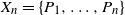
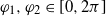
Let A be the centre of one of the circular discs, B and C the two intersection points of their boundaries, and D the midpoint of the segment connecting B and C, which coincides with the midpoint of the segment connecting the two centres; see Figure 2. By construction, $d(A,B) = r$ , $d(A,D) = t/2$ , and the angle ADB is $\pi/2$ . Let $\beta$ and $\alpha$ denote the angles DBA and BAC, respectively, and let $a=d(B,D)$ . We use spherical trigonometry in the triangle ABD. By the spherical sine theorem, $\sin \beta = \sin(t/2)/\sin r$ . By the spherical cosine theorem used for the side AB, $\cos r = \cos a \cos (t/2)$ , and for the side BD,

$$\cos(\alpha/2) = \frac{\cos a - \cos r \cos(t/2)}{\sin r \sin(t/2)} = \frac{\tan(t/2)}{\tan r}.$$

Figure 2. The surface area of the intersection of two spherical circular discs.

The surface area of half of the intersection is then obtained by subtracting the area of the triangle from the area of the circular sector, $\alpha\cdot(1-\cos r) - (\alpha + 2\beta - \pi)$ , which yields the assertions after substituting in the above formulas obtained for $\alpha$ and $\beta$ .

3. Proofs of Theorems 1 and 2

In the proof of Theorem 1, we closely follow the proof of the corresponding planar result in [Reference Fodor, Kevei and Vígh6, Theorem 1.2], whose argument is based on the technique used in [Reference Spivak17].

Proof of Theorem 1. Let $P_1$ and $P_2$ be two distinct points in K. There are exactly two spherical circular discs of radius r that contain both points in their boundaries. Let $D^{-}(P_1, P_2)$ and $D^{+} (P_1,P_2)$ denote the spherical disc-caps determined by these circular discs, i.e. the closure of the subset of K that is not covered by the corresponding disc. We also introduce the notation $A^{-}(P_1, P_2)= A(D^{-}(P_1, P_2))$ and $A^{+}(P_1, P_2)= A(D^{+} (P_1, P_2))$ . Furthermore, let $i(P_1, P_2)$ denote the length of the shorter r-arc connecting $P_1$ and $P_2$ .

The random pair of points $P_1,P_2\in K$ determines an edge of $K_n$ if and only if $D^{-}(P_1,P_2)$ or $D^{+}(P_1,P_2)$ don’t contain more of the chosen n points. Hence, our goal is to determine $\mathbb{E}(\operatorname{Per}(K)-\operatorname{Per}(K_n)) = \operatorname{Per}(K)-\binom n2\cdot I_n$ , where

$$ I_n = \frac{1}{A^2}\int\limits_{K}\int\limits_{K}\bigg(\bigg(1 -\frac{A^-(P_1,P_2)}{A}\bigg)^{n-2} + \bigg(1 -\frac{A^+(P_1,P_2)}{A}\bigg)^{n-2}\bigg)i(P_1,P_2)\,\mathrm{d}P_1\,\mathrm{d}P_2. $$

To compute this integral, we carry out the integral transformation in [Reference Nagy and Vígh14, Section 3], which can be described as follows. Let $\varrho=\varrho(s)$ be an arc-length parametrisation of $\partial K$ with positive orientation, and let $C=C(t,s)\in S^2$ be the point at distance $r+t$ from $\varrho(s)$ in the direction of $\varrho(s)\times \dot{\varrho}(s)$ along the great circle determined by the normal plane of $\partial K$ at $\varrho(s)$ . The normal plane is then the plane spanned by $\varrho(s)$ and $\varrho (s) \times \dot{\varrho}(s)$ , implying that

$$C = C(t,s)=\cos(r+t)\cdot \varrho(s) + \sin(r+t) \cdot \varrho(s)\times \dot \varrho(s).$$

Let $K_{t,s}$ denote the spherical circular disc with centre C(t, s) and radius r.

An orthonormal basis in the orthogonal complement of C is given by

\begin{equation*} w_1(t,s) \, :\!= \, \dot \varrho(s), \quad w_2(t,s) \, :\!= \, - \sin(r+t)\cdot \varrho(s) + \cos(r+t) \cdot \varrho(s)\times \dot \varrho(s). \end{equation*}

Any pair of points $(P_1, P_2)$ in K determines exactly two disc-caps, and by Lemma 2 each has a unique vertex $\varrho(s)$ and height t. Hence, the points can be reparametrised as

$$ P_i = \cos r\cdot C(t,s) + \sin r\cdot[\cos(\varphi_i)\cdot w_1(t,s) + \sin(\varphi_i)\cdot w_2(t,s)] $$

for some parameters $\varphi_1,\varphi_2\in [0,2\pi]$ . In general, this transformation is twofold, but because of the properties of the specific integrand here, every cap gets counted exactly twice.

Note that in this parametrisation, the area of the disc-cap is only dependent on t and s, and will be denoted by A(t, s), which is exactly the quantity defined in Lemma 3. Moreover, the circular arc connecting $P_1$ and $P_2$ has central angle $|\varphi_1-\varphi_2|$ in the plane in which it lies, and hence $i(P_1,P_2) = \sin r \cdot |\varphi_1-\varphi_2|$ .

Let t(s) denote the greatest value of t for which $K\cap K_{t,s}$ is nonempty, and let $[\theta_1, \theta_2]$ be the interval (depending on t and s) parametrising $\partial K_{t,s}\cap K$ . Then, by [Reference Nagy and Vígh14, Lemma 3], carrying out the above transformation yields

\begin{align*} I_n = \frac{1}{A^2}\int_{\partial K}\int_0^{t(s)}\int_{\theta_1}^{\theta_2}\int_{\theta_1}^{\theta_2} & \bigg(1-\frac{A(t,s)}{A}\bigg)^{n-2}\sin r|\varphi_1-\varphi_2| \\ & \times \sin^2 r(\sin(r+t)\kappa_\mathrm{g}-\cos(r+t))|\sin(\varphi_1-\varphi_2)|\, \mathrm{d}\varphi_1\,\mathrm{d}\varphi_2\,\mathrm{d}t\,\mathrm{d}s. \end{align*}

Note that $\kappa_\mathrm{g}=\kappa_\mathrm{g}(\varrho(s))$ is a function of s; however, we omit this from the notation to be as concise as possible. After integrating with respect to $\varphi_1$ and $\varphi_2$ , we obtain

\begin{align*} I_n = \frac{\sin^3 r}{A^2}\int_{\partial K}\int_0^{t(s)}&\bigg(1-\frac{A(t,s)}{A}\bigg)^{n-2} (\sin(r+t)\kappa_\mathrm{g}-\cos(r+t)) \\[5pt] & \times 2(2-\Delta\theta\sin\Delta\theta - 2\cos\Delta\theta)\, \mathrm{d}t\,\mathrm{d}s, \end{align*}

where $\Delta\theta \, :\!= \, \theta_2-\theta_1$ . This corresponds to the central angle $\Delta \theta = \Delta \theta (t,s)$ defined in Lemma 3.

We first show that $I_n$ is negligible on the interval $t\geq t'$ for arbitrary fixed $t'>0$ . It is clear that, for fixed s, the function A(t, s) is increasing in t; furthermore, it follows from a compactness argument that $\alpha \, :\!= \, \min_s A(t',s)>0$ , implying that $A(t,s)\geq \alpha$ for all s and $t\geq t'$ . Hence, the exponential term of the integrand can be upper bounded by $(1-\alpha/A)^{n-2}$ . The other terms can be bounded by a universal constant, again by a compactness argument, thus

\begin{align*} & n^{2/3}\binom{n}{2}\frac{\sin^3 r}{A^2}\int_{\partial K}\int_{t'}^{t(s)}\bigg(1-\frac{A(t,s)}{A}\bigg)^{n-2} (\sin(r+t)\kappa_\mathrm{g}(s)-\cos(r+t)) \\[5pt] & \qquad\qquad\qquad\qquad\qquad \times 2(2-\Delta\theta\sin\Delta\theta-2\cos\Delta\theta)\, \mathrm{d}t\,\mathrm{d}s \\[5pt] & \quad \leq Cn^{2/3}\binom n2\bigg(1-\frac{\alpha}{A}\bigg)^{n-2} \to 0 \quad \text{as } n\to\infty, \end{align*}

where C is some absolute constant. As a consequence, we aim to determine

$$ \lim_{n\to\infty}\mathbb{E}(\operatorname{Per}(K) - \operatorname{Per}(K_n))n^{2/3} = \lim_{n\to\infty}\bigg(\operatorname{Per}(K)-\binom n2\int_{\partial K}\hat I_n(s)\,\mathrm{d}s\bigg)n^{2/3}, $$

where

\begin{align*} \hat I_n(s) \, :\!= \, \frac{\sin^3 r}{A^2} \int_{0}^{t'} &\bigg(1-\frac{A(t,s)}{A}\bigg)^{n-2}(\sin(r+t)\kappa_\mathrm{g}-\cos(r+t)) \\ & \times 2(2-\Delta\theta\sin\Delta\theta - 2\cos\Delta\theta)\,\mathrm{d}t. \end{align*}

Fix $\varepsilon>0$ . We can choose $t'>0$ such that the following conditions hold for all $t\in[0,t']$ and all parameters s:

1. (i) $|\sin(r+t)\kappa_\mathrm{g}-\cos(r+t)-\sin r(\Delta\kappa_\mathrm{g} + t(1 + \cot^2 r + \cot r\Delta\kappa_\mathrm{g}))| < \varepsilon t$ by the first-order series expansion of the left-hand side;

2. (ii) $|A(t,s) - \big(v_1 t^{3/2} + v_2 t^{5/2}\big)| < \varepsilon t^{5/2}$ and

3. (iii) $1 \leq \left(1 - \dfrac{A(t,s)}{A}\right)^{-2} < 1 + \dfrac{3v_1}{A}t^{3/2}$ from the expansion of A(t, s) in Lemma 3;

4. (iv) $\bigg|2(2-\Delta\theta\sin\Delta\theta-2\cos\Delta\theta) - \dfrac{1}{6}\bigg(\vartheta_1^4t^2 + \bigg(4\vartheta_1^3\vartheta_2-\dfrac{\vartheta_1^6}{15}\bigg)t^3\bigg)\bigg| < \dfrac{\varepsilon}{6}t^3$ using the expansion of $\Delta\theta$ in Lemma 3, as well as the sixth-order Taylor polynomial $x^4/6 - x^6 / 90 + o(x^6)$ of $2(2 - x \sin x - 2 \cos x)$ ;

5. (v) $\bigg|\bigg(1 + \dfrac{3v_1}{A}t^{3/2}\bigg)(1+\cot^2 r+\cot r\kappa_\mathrm{g}\pm\varepsilon) \bigg(4\vartheta_1^3\vartheta_2-\dfrac{\vartheta_1^6}{15}\pm\varepsilon\bigg)t^4$

$\qquad +\ \dfrac{3v_1}{A}t^{3/2}\bigg[\Delta\kappa_\mathrm{g}\vartheta_1^4t^2 + \Delta\kappa_\mathrm{g}\bigg(4\vartheta_1^3\vartheta_2-\dfrac{\vartheta_1^6}{15}\pm\varepsilon\bigg)t^3$

$\qquad +\ \vartheta_1^4(1+\cot^2 r+\cot r\Delta\kappa_\mathrm{g}\pm\varepsilon)t^3\bigg]\bigg| < \varepsilon t^3$ ;

1. (vi) ${\mathrm{e}}^{-y}{\mathrm{e}}^{-(c+\varepsilon)y^{5/3}n^{-2/3}} \leq \bigg[1 - \dfrac{y}{n} - c\bigg(\dfrac{y}{n}\bigg)^{5/3}\bigg]^n \leq {\mathrm{e}}^{-y}{\mathrm{e}}^{-cy^{5/3}n^{-2/3}}$ and

2. (vii) ${\mathrm{e}}^{-(1+\varepsilon)y} \leq \bigg[1 - \dfrac{y}{n} - c\bigg(\dfrac{y}{n}\bigg)^{5/3}\bigg]^n \leq {\mathrm{e}}^{-(1-\varepsilon)y}$ for every $0 < y \leq n \min_s v_1(s) (t')^{2/3} /A$ and $c \in [- a, a]$ , with $a= A^{2/3} \max_s |v_2(s)/v_1^{5/3}(s)|$ .

We also choose $\delta= \delta(\varepsilon)$ small enough that, for all $|y| \leq \delta$ , ${\mathrm{e}}^{-y} \leq 1 - (1-\varepsilon)y$ . Lastly, let $n_0$ be large enough that

$$ \max_s\frac{|v_2(s)|A^{2/3}}{v_1^{5/3}(s)n_0^{1/3}} \leq \delta, \qquad \max_s\frac{(1-\varepsilon)(v_2(s)-\varepsilon)A^{2/3}D_2^\varepsilon}{v_1^{7/3}(s)n_0^{3/5}} \leq \varepsilon, $$

with $D_2^\varepsilon$ defined by (4). By assumptions (i)–(v),

\begin{align*} \hat I_n(s) & \leq \frac{\sin^4 r}{6A^2}\int_0^{t'}\bigg(1-\frac{A(t,s)}{A}\bigg)^n \big(\Delta\kappa_\mathrm{g} + (1+\cot^2 r+\cot r\Delta\kappa_\mathrm{g}+\varepsilon)t\big) \\ &\;\;\qquad\quad \qquad \times \bigg(\vartheta_1^4t^2 + \bigg(4\vartheta_1^3\vartheta_2-\frac{\vartheta_1^6}{15}+\varepsilon\bigg)t^3\bigg) \bigg(1 + \frac{3v_1}{A}t^{3/2}\bigg)\,\mathrm{d}t \\ & \leq \frac{\sin^4r}{6A^2}\int_0^{t'}\bigg(1-\frac{v_1}{A}t^{3/2}-\frac{v_2-\varepsilon}{A}t^{5/2}\bigg)^n \big(D_1t^2 + D_1D_2^\varepsilon t^3\big)\,\mathrm{d}t, \end{align*}

where

(4) \begin{equation} D_1 = \Delta\kappa_\mathrm{g}\vartheta_1^4, \ D_1D_2^\varepsilon = \vartheta_1^4(1 + \cot^2 r + \cot r\Delta\kappa_\mathrm{g} + \varepsilon) + \Delta\kappa_\mathrm{g}\bigg(4\vartheta_1^3\vartheta_2 - \frac{\vartheta_1^6}{15}+\varepsilon\bigg) + \varepsilon. \end{equation}

Using the substitution $t^{3/2} v_1 /A= y/n$ , we have

$$ \hat I_n(s) \leq \frac{\sin^4 rD_1}{9n^2v_1^2}\int_0^{n t''} \bigg[1 - \frac{y}{n} - \frac{(v_2-\varepsilon)A^{2/3}}{v_1^{5/3}}\bigg(\frac yn\bigg)^{5/3}\bigg]^n \bigg[1 + D_2^\varepsilon\bigg(\frac{Ay}{nv_1}\bigg)^{2/3}\bigg]y\,\mathrm{d}y, $$

where $t''\, :\!= \, (t')^{3/2} v_1 /A$ .

We consider the integral on the interval $[n^{1/5},nt'']$ first. As $D_2^\varepsilon$ has a uniform upper bound, and $v_1$ a uniform (nonzero) lower bound, for large enough n the second factor is at most 2. Using assumption (vii), the expression is upper bounded by

$$ \frac{2\sin^4rD_1}{9n^2v_1^2}\int_{n^{1/5}}^{nt''}{\mathrm{e}}^{-(1-\varepsilon)y} nt''\,\mathrm{d}y \leq \frac{2\sin^4rD_1}{9nv_1^2}{\mathrm{e}}^{-(1-\varepsilon)n^{1/5}}, $$

which tends to zero faster than any polynomial of n, and hence tends to zero when multiplied by $\binom n2\cdot n^{2/3}$ .

For the integral on $[0,n^{1/5}]$ we use assumption (v), and the choice of $\delta$ and $n_0$ , to obtain the following upper bound for $n\geq n_0$ :

\begin{eqnarray*} &&\frac{\sin^4rD_1}{9n^2v_1^2}\int_0^{n^{1/5}}{\mathrm{e}}^{-y}\exp\bigg\{{-}\frac{(v_2-\varepsilon)A^{2/3}}{v_1^{5/3}} \frac{y^{5/3}}{n^{2/3}}\bigg\}\bigg[1+D_2^\varepsilon\bigg(\frac{Ay}{nv_1}\bigg)^{2/3}\bigg]y\,\mathrm{d}y \\[10pt]&&\quad\leq \frac{\sin^4rD_1}{9n^2v_1^2}\int_0^{n^{1/5}}{\mathrm{e}}^{-y} \bigg(1-(1-\varepsilon)\frac{(v_2-\varepsilon)A^{2/3}}{v_1^{5/3}}\frac{y^{5/3}}{n^{2/3}}\bigg) \bigg[1+D_2^\varepsilon\bigg(\frac{Ay}{nv_1}\bigg)^{2/3}\bigg]y\,\mathrm{d}y. \end{eqnarray*}

Multiplying out the product, and again using the choice of $n_0$ , we obtain the upper bound

$$ \frac{\sin^4rD_1}{9n^2v_1^2}\int_0^{n^{1/5}}{\mathrm{e}}^{-y} \bigg[1+\frac{A^{2/3}}{n^{2/3}}\bigg(\frac{D_2^\varepsilon}{v_1^{2/3}}y^{2/3} - (1-\varepsilon)\frac{(v_2-\varepsilon)}{v_1^{5/3}}y^{5/3} + \varepsilon\bigg)\bigg]y\,\mathrm{d}y. $$

Expanding the domain of the integration, and using the definition of the Gamma function, we get the bound

$$ \frac{\sin^4rD_1}{9n^2v_1^2}\bigg[1 + \frac{A^{2/3}}{n^{2/3}}\bigg(\frac{D_2^\varepsilon}{v_1^{2/3}}\Gamma\bigg(\frac83\bigg) - (1-\varepsilon)\frac{v_2-\varepsilon}{v_1^{5/3}}\Gamma\bigg(\frac{11}{3}\bigg) + 2\varepsilon\bigg)\bigg]. $$

We can obtain a lower bound in a similar way, and as $\varepsilon$ was arbitrary, $\hat I_n(s)$ is asymptotically equal to this formula with $\varepsilon=0$ .

If we write in the formulas for $D_1$ and $v_1$ , we see that $\sin^4 r D_1/(18v_1^2) = 1$ , and since $\int_{\partial K} 1\,\mathrm{d}s = \operatorname{Per}(K)$ , in the limit the perimeter cancels out, hence

\begin{align*} \lim_{n\to\infty}\mathbb{E}(\operatorname{Per}(K)-\operatorname{Per}(K_n))n^{2/3} & = \lim_{n\to\infty}\bigg(\operatorname{Per}(K)-\binom n2\int_{\partial K}\hat I_n(s)\,\mathrm{d}s\bigg)n^{2/3} \\ & = \int_{\partial K}\frac{\sin^4rD_1A^{2/3}}{18v_1^2} \bigg(\frac{v_2}{v_1^{5/3}}\Gamma\bigg(\frac{11}{3}\bigg) - \frac{D_2}{v_1^{2/3}}\Gamma\bigg(\frac83\bigg)\bigg)\,\mathrm{d}s. \end{align*}

After expanding the formulas (see also [Reference Nagy and Vígh15]), we obtain that the limit of the expectation is finally equal to

\begin{eqnarray*}&& \sqrt[\ 3\ ]{\frac{2A^2}{3}}\Gamma\bigg(\frac53\bigg)\frac14\int_{\partial K} \Delta\kappa_\mathrm{g}^{1/3}(3\Delta\kappa_\mathrm{g}+4\cot r) - \frac{5(\kappa_\mathrm{g}')^2-3\kappa_\mathrm{g}''\Delta\kappa_\mathrm{g}}{3\Delta\kappa_\mathrm{g}^{8/3}}\, \mathrm{d}s \\&&\quad = \sqrt[\ 3\ ]{\frac{2A^2}{3}}\Gamma\bigg(\frac53\bigg)\frac14\int_{\partial K} \Delta\kappa_\mathrm{g}^{1/3}(3\kappa_\mathrm{g}+\cot r) - \frac{5(\kappa_\mathrm{g}')^2 - 3\kappa_\mathrm{g}''\Delta\kappa_\mathrm{g}}{3\Delta\kappa_\mathrm{g}^{8/3}}\, \mathrm{d}s. \end{eqnarray*}

By an elementary calculation, the last term in the integral is exactly the derivative of the expression $\kappa_\mathrm{g}'/\Delta\kappa_\mathrm{g}^{5/3}$ , and hence its integral is zero. The remaining expression is exactly the statement of the theorem.

Proof of Theorem 2. In the case when K is the circular disc of radius r, we follow similar steps. The integral transformation used is geometrically similar to the previous one, and its Jacobian is given by [Reference Nagy and Vígh14, Lemma 1], hence we obtain

\begin{align*}\lim_{n\to\infty}\mathbb{E}(\operatorname{Per}(K_n)) = \lim_{n\to\infty}\binom{n}{2}\frac{2\sin^3r}{A^2}\int_0^{t'} & \bigg(1-\frac{A(t)}{A}\bigg)^n\nonumber\\[8pt] &\times\sin t\cdot(2-\Delta\theta\sin\Delta\theta - 2\cos\Delta\theta)\,\mathrm{d}t, \end{align*}

where $A\, :\!= \,\operatorname{SArea}(K) = 2\pi(1-\cos r)$ , and the upper bound of the integral t ^′ is some sufficiently small fixed number. Using the appropriate series expansions, we obtain that the integral is of the form

$$ \int_0^{t'}\bigg(1-\frac{2\sin r}{A}t + \frac{\cot r\cos r}{12A}t^3 + O(t^5)\bigg)^n \bigg(t-\frac{t^3}{6} + O(t^5)\bigg)(4-\pi\cot r\cdot t + O(t^3))\,\mathrm{d}t. $$

Using similar analytical tools as above, we obtain the statement of the theorem.

4. Duality

We define the spherical r-convex dual of the set

\begin{align*}H \text{ as } H^r=\{y\in S^2 \mid H\subseteq B(y,r)\} = \bigcap_{x\in H} B(x,r). \end{align*}

As discussed in the introduction, this operation reverses inclusion, and if $H=K$ is an r-spindle convex disc, $K = (K^r)^r$ , justifying the name ‘duality’. If K has a $C^1$ boundary, then for any $x=\varrho(s)\in \partial K$ , the smoothness guarantees that there is a unique point, denoted by $x^r\, :\!= \,x^r(s)$ , such that the spherical circular disc with centre $x^r$ and radius r supports K at x, i.e. $B(x^r,r)$ contains K, and their supporting great circles at x coincide (see Figure 3). By the definition of the dual set, $x^r\in K^r$ , and more specifically it is a boundary point. It is also straightforward to check that $(x^r)^r=x$ .

Figure 3. The spherical spindle convex dual.

We note that in the special case of $r=\pi/2$ , it is easy to see that $K^{\pi/2}=-K^\circ$ , where $K^\circ = \{y\in S^2 \mid \langle y, x\rangle \leq 0\ \text{for all}\ x\in K\}$ is the spherical polar body.

1. (i) $\operatorname{Per}(K^r) = \sin r\cdot2\pi - \cos r\cdot\operatorname{Per}(K) - \sin r\cdot\operatorname{SArea}(K)$ , and

2. (ii) $\operatorname{SArea}(K^r) = (1-\cos r)\cdot2\pi - \sin r\cdot\operatorname{Per}(K) + \cos r\cdot\operatorname{SArea}(K)$ .

Furthermore, if K has a $C^2$ boundary with the property that $\kappa_\mathrm{g}(x) > \cot r$ for every $x\in \partial K$ , the equality

1. (iii) $\sin^2 r \cdot (\kappa_\mathrm{g}^r(x^r)-\cot r)(\kappa_\mathrm{g}(x)-\cot r)=1$ also holds, where $\kappa_\mathrm{g}^r(y)$ denotes the geodesic curvature of $\partial K^r$ at a point y.

Proof. First, we assume K is of class $C^2$ and $\kappa_\mathrm{g}>\cot r$ , and let $\varrho = \varrho(s)$ be an arc-length parametrisation of $\partial K$ with positive orientation. Then the centre $x^r$ of the support r-disc at $x = \varrho(s) \in \partial K$ can be explicitly determined using the parametrisation of $\partial K$ , namely

$$x^r = \cos r \cdot \varrho(s) + \sin r \cdot \varrho(s) \times \dot{\varrho}(s).$$

Hence, a parametrisation of $\partial K^r$ is given by

(5) \begin{equation} \zeta(s) = \cos r\cdot\varrho(s) + \sin r\cdot\varrho(s)\times\dot{\varrho}(s), \quad s\in [0,\operatorname{Per}(K)]. \end{equation}

Differentiating and using the relationship $\ddot{\varrho}=\kappa_\mathrm{g}\cdot\varrho\times\dot{\varrho}-\varrho$ from Lemma 1, we obtain that $\dot{\zeta}(s) = -\dot{\varrho}(s) \cdot \sin r \cdot (\kappa_\mathrm{g}(\varrho(s)) - \cot r)$ . Hence,

\begin{align*} \operatorname{Per}(K^r) = \int_0^{\operatorname{Per}(K)}|\dot{\zeta}(s)|\,\mathrm{d}s & = \int_0^{\operatorname{Per}(K)}\sin r(\kappa_\mathrm{g}(\varrho(s))-\cot r)\,\mathrm{d}s \\ & = \sin r\int_0^{\operatorname{Per}(K)}\kappa_\mathrm{g}(\varrho(s))\,\mathrm{d}s - \cos r\cdot\operatorname{Per}(K), \end{align*}

and as the Gaussian curvature of $S^2$ is constant 1, by the Gauss–Bonnet theorem we have

$$ \int_0^{\operatorname{Per}(K)}\kappa_\mathrm{g}(\varrho(s))\,\mathrm{d}s = 2\pi - \int_K1\,\mathrm{d}A = 2\pi - \operatorname{SArea}(K), $$

which yields the first part of the assertion. Since $(K^r)^r = K$ , using the corresponding formula for $K\, :\!= \,K^r$ and some algebraic manipulations, we obtain the second expression.

To obtain the formula for the geodesic curvature, we first find an expression for the curvature $\kappa^r$ of $\partial K^r$ . To do this, we use the standard differential geometry formula

$$\kappa^r(\zeta(s)) = \frac{|\dot \zeta (s)\times \ddot \zeta(s)| }{|\dot{\zeta}(s)|^3}.$$

From (5), we see that

\begin{align*} \ddot{\zeta}(s) & = -\ddot{\varrho}(s)\cdot\sin r\cdot(\kappa_\mathrm{g}(\varrho(s))-\cot r) - \dot{\varrho}(s)\cdot\sin r\cdot\kappa_\mathrm{g}'(\varrho(s)) \\ & = -(\kappa_\mathrm{g}(\varrho(s))\cdot\varrho\times\dot{\varrho} - \varrho)\cdot\sin r \cdot (\kappa_\mathrm{g}(\varrho(s))-\cot r) - \dot{\varrho}(s)\cdot\sin r\cdot\kappa_\mathrm{g}'(\varrho(s)), \end{align*}

and hence $\dot{\zeta}(s)\times\ddot{\zeta}(s) = \sin^2r(\kappa_\mathrm{g}(\varrho(s))-\cot r)^2\cdot (\kappa_\mathrm{g}(\varrho(s))\cdot\varrho(s) - \varrho(s)\times\dot{\varrho}(s))$ , implying that its length is

$$ \sin^2r(\kappa_\mathrm{g}(\varrho(s))-\cot r)^2\cdot\big(\kappa_\mathrm{g}^2(\varrho(s))+1\big)^{1/2} = \sin^2r(\kappa_\mathrm{g}(\varrho(s))-\cot r)^2\kappa(\varrho(s)), $$

and thus

$$\kappa^r(\zeta(s)) = \frac{\kappa(\varrho(s))}{\sin r \cdot (\kappa_\mathrm{g}(\varrho(s))-\cot r)}.$$

Since $(x^r)^r=x$ , we can express $\kappa(\varrho(s))$ in terms of $\kappa^r(\zeta(s))$ in a similar way, which yields the desired equality.

As the duality transformation is continuous, for general K we can obtain the results for surface area and perimeter by using standard approximating tools.

We note that if we consider the perimeter and surface area as special intrinsic volumes, the case for the polar body follows from combining Theorem 4.3.1 and Corollary 4.3.3 of [Reference Glasauer10] in dimension 2.

Lemma 6. Let K be a spherical spindle convex disc with $C^2$ boundary and with the property that $\kappa_\mathrm{g}(x)>\cot r$ for every $x\in \partial K$ . Then

$$ \int_{\partial K^r}F\big(\Delta\kappa_\mathrm{g}^r\big)\,\mathrm{d}s = \int_{\partial K}F\bigg(\frac{1}{\sin^2 r\Delta\kappa_\mathrm{g}}\bigg)\cdot \sin r\cdot\Delta\kappa_\mathrm{g}\,\mathrm{d}s $$

for any integrable function F, where the integration is taken with respect to arc length on both sides, $\Delta\kappa_\mathrm{g} \, :\!= \, \kappa_\mathrm{g} - \cot r$ , $\Delta\kappa_\mathrm{g}^r \, :\!= \, \kappa_\mathrm{g}^r-\cot r$ , and $\kappa_\mathrm{g}$ ( $\kappa_\mathrm{g}^r$ ) is understood as $\kappa_\mathrm{g}(\varrho(s))$ ( $\kappa_\mathrm{g}^r(\hat\varrho(s))$ ) if $\varrho(s)$ ( $\hat\varrho(s)$ ) is an arc-length parametrisation of $\partial K$ ( $\partial K^r$ ).

We find the Jacobian as follows. The ratio of the arc lengths of $\partial K^r$ and $\partial K$ between the points $\zeta(s)$ , $\zeta(s+h)$ and $\varrho(s)$ , $\varrho(s+h)$ , respectively, is

$$ \frac{1}{h}\cdot\int_{s}^{s+h}|\dot{\zeta}(\tau)|\,\mathrm{d}\tau = \frac{1}{h}\cdot\int_{s}^{s+h}\sin r\cdot(\kappa_\mathrm{g}(\varrho(\tau))-\cot r)\,\mathrm{d}\tau. $$

The limit of this expression as $h \to 0$ is, by definition,

$$ \frac{\mathrm{d}}{\mathrm{d}h}\int_{s}^{s+h}\sin r\cdot(\kappa_\mathrm{g}(\varrho(\tau))-\cot r)\,\mathrm{d}\tau = \sin r\cdot(\kappa_\mathrm{g}(\varrho(s))-\cot r), $$

where we used the Leibniz integral rule to obtain the formal derivative.

5. A circumscribed model

In this section, we prove the asymptotic formulae stated in Theorem 3, regarding the expectation of the area and perimeter deviations of a spherical spindle convex disc K and a circumscribed spherical disc–polygon $K_{(n)}$ . Recall that $K_{(n)}$ is obtained by taking the spherical spindle convex dual of the spherical spindle convex hull of n uniformly distributed, independent points chosen from $K^r$ .

By Lemma 5, we have

(6) \begin{equation} \begin{aligned} \operatorname{Per}(K_{(n)}) - \operatorname{Per}(K) & = \cos r\cdot\big(\operatorname{Per}\big(K^r\big)-\operatorname{Per}\big(K_{(n)}^r\big)\big) + \sin r\cdot\operatorname{SArea}\big(K^r\setminus K_{(n)}^r\big), \\ \operatorname{SArea}\big(K_{(n)}\setminus K\big) & = \sin r\cdot\big(\operatorname{Per}(K^r)-\operatorname{Per}\big(K_{(n)}^r\big)\big) - \cos r\cdot\operatorname{SArea}\big(K^r\setminus K_{(n)}^r\big), \end{aligned}\end{equation}

and, by definition, $K^r_{(n)}$ is a uniform disc–polygon in $K^r$ .

To be concise, we use the notation $\Delta\kappa_\mathrm{g}(s) = \kappa_\mathrm{g}(s)-\cot r$ as previously, and $\Delta\kappa_\mathrm{g}^r(s) = \kappa_\mathrm{g}^r(s)-\cot r$ for the dual disc, as well as $A(\!\cdot\!)$ for $\operatorname{SArea}(\!\cdot\!)$ . From (1), and using the integral transformation in Lemma 6, we obtain

\begin{align*} \lim_{n\to\infty}\mathbb{E}\big(\!\operatorname{SArea}\big(K^r \setminus K_{(n)}^r\big)\big) \cdot n^{2/3} & = \sqrt[\ 3\ ]{\frac{2A(K^r)^2}{3}}\Gamma\bigg(\frac53\bigg) \int_{\partial K^r}\big(\Delta\kappa_\mathrm{g}^r(s)\big)^{1/3}\,\mathrm{d}s \\[8pt] & = \sqrt[\ 3\ ]{\frac{2A(K^r)^2}{3}}\Gamma\bigg(\frac53\bigg) \int_{\partial K}\bigg(\frac{1}{\sin^2 r\Delta\kappa_\mathrm{g}}\bigg)^{1/3}\sin r\Delta\kappa_\mathrm{g}\, \mathrm{d}s \\[8pt] & = \sqrt[\ 3\ ]{\frac{2A(K^r)^2}{3}}\Gamma\bigg(\frac53\bigg)(\!\sin r)^{1/3} \int_{\partial K}\Delta\kappa_\mathrm{g}^{2/3}\,\mathrm{d}s.\end{align*}

Similarly, from Theorem 1 we have

\begin{align*} & \lim_{n\to\infty}\mathbb{E}\big(\!\operatorname{Per}(K^r) - \operatorname{Per}\big(K_{(n)}^r\big)\big)\cdot n^{2/3} \\[8pt] & \qquad = \sqrt[\ 3\ ]{\frac{2A(K^r)^2}{3}}\Gamma\bigg(\frac53\bigg)\int_{\partial K^r} \big(\Delta\kappa_\mathrm{g}^r\big)^{1/3}\cdot\bigg(\frac34\Delta\kappa_\mathrm{g}^r + \cot r\bigg)\,\mathrm{d}s \\[8pt] & \qquad = \sqrt[\ 3\ ]{\frac{2A(K^r)^2}{3}}\Gamma\bigg(\frac53\bigg)\int_{\partial K} \bigg(\frac{1}{\!\sin^2r\Delta\kappa_\mathrm{g}}\bigg)^{1/3} \bigg(\frac{3}{4\sin^2r\Delta\kappa_\mathrm{g}} + \cot r\bigg)\sin r\Delta\kappa_\mathrm{g}\,\mathrm{d}s \\ & \qquad = \sqrt[\ 3\ ]{\frac{2A(K^r)^2}{3}}\Gamma\bigg(\frac53\bigg)(\sin r)^{1/3}\int_{\partial K} \Delta\kappa_\mathrm{g}^{2/3}\bigg(\frac{3}{4\sin^2r\Delta\kappa_\mathrm{g}} + \cot r\bigg)\,\mathrm{d}s.\end{align*}

Combining these results with (6), we have

\begin{eqnarray*} && \lim_{n\to\infty}\mathbb{E}(\!\operatorname{SArea}(K_{(n)}\setminus K))n^{2/3} \\ &&\qquad =\sqrt[\ 3\ ]{\frac{2A(K^r)^2}{3}}\Gamma\bigg(\frac53\bigg)(\!\sin r)^{1/3}\int\limits_{\partial K} \Delta\kappa_\mathrm{g}^{2/3}\bigg(\sin r\bigg(\frac{3}{4\sin^2r\Delta\kappa_\mathrm{g}} + \cot r\bigg) - \cos r\bigg)\,\mathrm{d}s , \end{eqnarray*}

and

\begin{eqnarray*} && \lim_{n\to\infty}\mathbb{E}(\!\operatorname{Per}(K_{(n)}-\operatorname{Per}(K))n^{2/3} \\ &=& \sqrt[\ 3\ ]{\frac{2A(K^r)^2}{3}}\Gamma\bigg(\frac53\bigg)(\!\sin r)^{1/3}\int\limits_{\partial K} \Delta\kappa_\mathrm{g}^{2/3}\bigg(\cos r\bigg(\frac{3}{4\sin^2r\Delta\kappa_\mathrm{g}} + \cot r\bigg) + \sin r\bigg)\,\mathrm{d}s, \end{eqnarray*}

which yield the desired formulas after simplification of the integrand, and substituting $A(K^r)$ with $(1-\cos r)2\pi - \sin r \operatorname{Per}{(K)} + \cos r A(K)$ from Lemma 5.