

INTRODUCTION
The Arctic sea-ice cover and its changes in recent years are one of the most visible signs of climate change. Sea-ice extent has decreased dramatically in the last decades, ~10.8% per decade for the minimum ice extent over the period 1979–2015, and a thinning of the ice cover of ~0.6 m per decade over the period 2000–12 has also been observed (Lindsay and Schweiger, Reference Lindsay and Schweiger2015; Serreze and Stroeve, Reference Serreze and Stroeve2015; Comiso and others, Reference Comiso, Meier and Gersten2017). For a better understanding of the ongoing changes and their relevance to the local and global climate, a more detailed knowledge of the sea-ice cover is necessary, especially to capture the effects of small-scale features like leads (Marcq and Weiss, Reference Marcq and Weiss2012; Vihma, Reference Vihma2014). The retreating sea ice also attracts more ship traffic to the polar ocean for exploration, exploitation, research and tourism (Eguíluz and others, Reference Eguíluz, Fernández-Gracia, Irigoien and Duarte2016). Safe navigation in ice-infested waters demands high resolution and timely information of the actual sea-ice situation.
Fram Strait, located between Svalbard and Greenland, is the main gateway to the Arctic Ocean and plays an important role in the sea-ice mass balance of the Arctic. The majority of the exported sea ice is transported through this strait by the East Greenland Current while comparatively warm Atlantic Water is brought into the Arctic basin by the West Spitzbergen Current (Kwok and others, Reference Kwok, Spreen and Pang2013; Carmack and others, Reference Carmack2015; Smedsrud and others, Reference Smedsrud, Halvorsen, Stroeve, Zhang and Kloster2017). The sea-ice cover in this region is highly dynamic. In particular, the marginal ice zone (MIZ), i.e. the transition between the closed pack ice and the open ocean, is exposed to rapid changes induced by wind and currents due to lower ice concentration (e.g. Shuchman and others, Reference Shuchman1987). To cover these dynamic sea-ice processes, observations with high spatial and temporal resolution are necessary.
While passive microwave radiometry offers a long-term and consistent record of sea-ice parameters, for example concentration and extent, since 1978, its low resolution is not suitable for studying small-scale features especially in the MIZ (Meier and others, Reference Meier, Peng, Scott and Savoie2014). Optical sensors, on the other hand, offer high spatial resolution but the imagery is hampered by clouds and the polar night. Synthetic aperture radar (SAR) combines a resolution of ~100 m for wide swath images with a coverage of the entire Arctic in a few days. For some parts of the Arctic, for example Fram Strait to Franz Josef Land, daily coverage is common. Operating in the microwave region of the electromagnetic spectrum, SAR images are almost unaffected by atmospheric conditions and offer a day-and-night year-round imaging capability due to the active nature of the sensor.
To date, operational ice charts are based on the manual interpretation of available data sources, but efforts have been made to automatize the retrieval of sea-ice parameters. SAR imagery has been employed for instance for sea-ice classification (e.g. Zakhvatkina and others, Reference Zakhvatkina, Alexandrov, Johannessen, Sandven and Frolov2012), ice concentration (e.g. Wang and others, Reference Wang, Scott and Clausi2017) and sea-ice drift estimation (e.g. Korosov and Rampal, Reference Korosov and Rampal2017; Lehtiranta and others, Reference Lehtiranta, Siiriä and Karvonen2015). C-band (wavelength 3.75–7.5 cm) is the preferred frequency used for operational monitoring of sea ice with SAR as it offers good discrimination between ice types and ice water contrast during summer (Carsey, Reference Carsey1992; Geldsetzer and others, Reference Geldsetzer2015). But studies have shown that other frequencies, mainly X- (wavelength 2.5–3.75 cm) and L-band (15– 30 cm), add complementary information that can aid interpretation of the images and retrieval of sea-ice parameters (Johansson and others, Reference Johansson2017; Eriksson and others, Reference Eriksson2010). Dierking and Busche (Reference Dierking and Busche2006) demonstrate the usefulness of L-band data in identifying floe boundaries and deformation features such as ridges, shear zones and rubble fields, while a study by Casey and others (Reference Casey, Howell, Tivy and Haas2016) underlines the capabilities of L-band during the melt season.
The use of dual-polarization imagery eases the distinction between ice and water (Scheuchl and others, Reference Scheuchl, Flett, Caves and Cumming2004). While for the co-polarization channel the backscatter of open water highly depends on wind speed, wind direction and incidence angle and can reach the values of sea ice, this effect is largely reduced for the cross-polarization channel and nearly independent from the incidence angle (Isoguchi and Shimada, Reference Isoguchi and Shimada2009; Horstmann and others, Reference Horstmann2015). Backscatter alone has proven not to be sufficient for reliable and accurate image interpretation over a wide range of incidence angles and changing ambient conditions (Karvonen, Reference Karvonen2014). Texture measures are widely used as additional image features as they do not only take the brightness into account, but also its spatial variation (Shokr, Reference Shokr1991; Haralick and others, Reference Haralick, Shanmugam and Dinstein1973). Texture features derived from grey-level co-occurrence matrices (GLCM) have been used in a number of sea-ice classification algorithms (Soh and Tsatsoulis, Reference Soh and Tsatsoulis1999; Clausi, Reference Clausi2002; Zakhvatkina and others, Reference Zakhvatkina, Korosov, Muckenhuber, Sandven and Babiker2017). Autocorrelation is another texture feature which has proven capabilities in ice-water discrimination and ice concentration estimation (Karvonen and others, Reference Karvonen, Simila and Makynen2005; Berg and Eriksson, Reference Berg and Eriksson2012; Karvonen, Reference Karvonen2012).
In this paper, we present a comparison of sea ice/open water maps of Fram Strait derived from spaceborne C- and L-band SAR imagery. We use wide swath SAR data from two currently operating satellite missions: Sentinel-1, a C-band SAR operated by the European Space Agency (ESA) within the scope of the Copernicus programme, and ALOS-2 PALSAR-2, a L-band mission operated by the Japan Aerospace Exploration Agency (JAXA). All images are dual-polarization, i.e both horizontal transmit and receive (HH) and horizontal transmit and vertical receive (HV) bands are available. While C-band SAR imagery is widely used for sea-ice analysis and currently provided by two missions (Sentinel-1, Radarsat-2), ALOS-2 PALSAR-2 is the only spaceborne L-band SAR currently in operation. To the best of our knowledge, this is the first time that ALOS-2 PALSAR-2 ScanSAR data are evaluated for sea-ice monitoring. Fully polarimetric, i.e transmission and reception of both horizontal and vertical polarizations, ALOS-2 PALSAR-2 data with smaller spatial coverage (50 km swath width) have been used for sea-ice studies (Johansson and others, Reference Johansson2017, Reference Johansson, Brekke, Spreen and King2018).
The main objective of the work presented here is to study the information differences between the two frequencies and their consequences on the derived ice/water maps and the potential benefits of combining the two frequencies to obtain more accurate results.
The challenge for classification of wide swath imagery is the variety of covered ice regimes within a scene, the variability of backscatter properties with ambient conditions over ice and open water, and the incidence angle dependence of the backscatter intensities. Machine learning techniques are state-of-the-art for such image classification. Hence, in our study, we use a feed-forward neural network to achieve the mapping between image features, i.e brightness information, texture features and incidence angle, and the output classes. Neural networks have been successfully used in a number of studies on the sea-ice classification, (e.g. Berg and Eriksson, Reference Berg and Eriksson2012; Karvonen, Reference Karvonen2014; Ressel and others, Reference Ressel, Frost and Lehner2015). Once trained they can be applied to any SAR image to obtain a classified image. Furthermore, new features can be easily integrated into a network. It is a supervised learning method and hence for the training of the network, a training dataset with correct classes is needed. We used manually defined regions of ice and water for the training process.
One network has been trained for each frequency separately to accommodate the different backscatter levels.
SATELLITE IMAGERY AND VALIDATION DATA
Satellite imagery
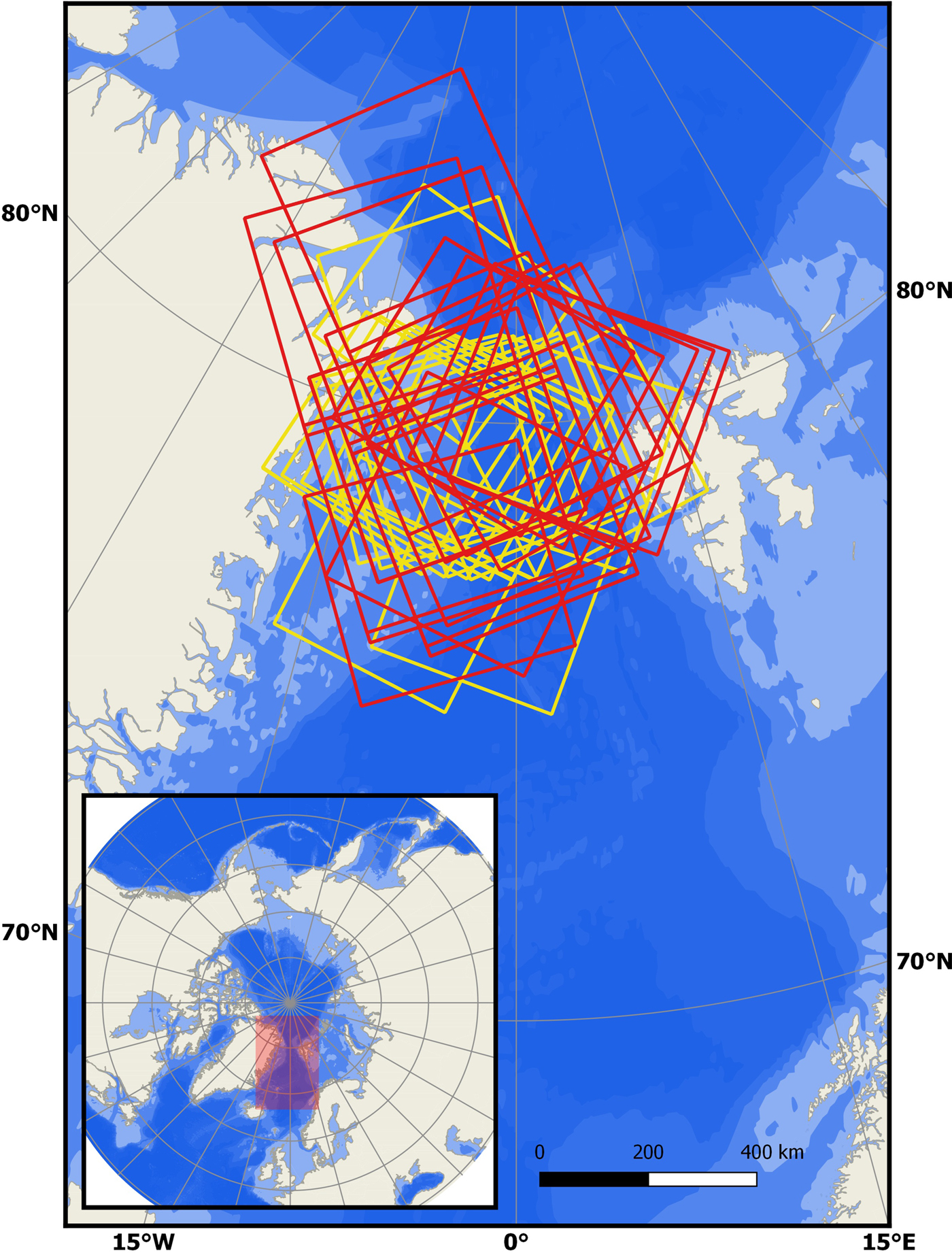
Figure 1 shows the geographical location of the study area in Fram Strait between Greenland and Svalbard. The outlines of the used images from the spaceborne SAR sensors ALOS-2 PALSAR-2 (L-band) and Sentinel-1 (C-band) are shown in yellow and red, respectively. The goal of this study is the evaluation of C- and L-band images for ice/water classification. Therefore, a set of six near-coincidental image pairs is included in the dataset. Acquisition times between the two sensors for these pairs differ by 2--3 hours and different orbit directions, i.e. on descending orbit for ALOS-2 PALSAR-2 and on ascending orbit for Sentinel-1. This implies that near and far range is at different image locations and features are seen from different viewing angles for the two frequencies. The incidence angle dependence is especially pronounced over open water and hence, the backscatter over open ocean is differently affected at the two frequencies. A detailed description of the utilized imagery and validation data is given below.
Study area with PALSAR-2 images in yellow and Sentinel-1 images in red. Coastline from OpenStreetMap (http://openstreetmapdata.com/data/coastlines). Bathymetry (0, 200, 1000, 2000, 3000, 4000 m) from naturalearthdata.com.
Sentinel-1 C-band
Copernicus' Sentinel-1 mission, a constellation of two C-band SAR satellites with dual polarization capabilities, offers a coverage of the entire Arctic within a few days and an exact revisit time of 6 days. Images over Fram Strait are usually acquired daily. The data are freely available from the Copernicus Open Access Hub (https://scihub.copernicus.eu/). Twenty-five images, acquired during the period from October 2015 to March 2016 over Fram Strait, have been used for algorithm development and verification. Data before October 2015 have not been considered due to the noise calibration not been working efficiently then. The images are level-1 ground range detected (GRD) products, i.e. detected, multi-looked and projected to the ground range, in Extra Wide (EW) swath mode with medium resolution and dual polarization (HH - horizontal transmit and receive and HV - horizontal transmit and vertical receive). The swath width is ~400 km and the resolution is ~90 m with a pixel size of 40 m (see Table 1).
Parameters of the SAR sensors and operation modes used in this study

* Noise equivalent sigma zero.
The data have been preprocessed with the Sentinel Application Platform (SNAP) according to the following processing chain: apply orbit file - thermal noise removal - calibration - projection to UTM Zone 30N. The images have been calibrated to γ 0:
 $$\gamma _0 = \displaystyle{{\sigma _0} \over {\cos \theta _{inc}}}$$
with backscatter intensity σ 0 and incidence angle θ inc, to account for variations of the backscatter intensity with incidence angle. Hereafter γ 0 is termed backscatter intensity. To achieve a good spatial overlap with the L-band data at some occasions, two Sentinel-1 images from the same orbit have been sliced together. Apply orbit file and removal of Boarder Noise was applied to the individual images and the same processing chain as above was followed after the slicing operation.
ALOS-2 PALSAR-2 L-band
L-band imagery from the ALOS-2 PALSAR-2 sensor was acquired from the Japan Aerospace Exploitation Agency (JAXA) in ScanSAR Wide Beam Dual (WBD) mode. The images are level 1.5 data which are multi-looked and geocoded. The images have a swath width of 350 km and a resolution of ~90 m with a pixel size of 25 m (see Table 1). The data are dual polarization data in HH and HV. ALOS-2 PALSAR-2 provides an exact revisit time of 14 days, but data over the Arctic is more scarce and not available for every date due to the acquisition plan. The images have been calibrated to γ 0 using the provided calibration factors and formulas and the incidence angle which can be derived from the product metadata (JAXA, 2017). The images have been resized to 40 m pixel size and projected to UTM Zone 30N to be comparable with the Sentinel-1 C-band data. Twenty four images acquired between October 2014 and February 2016 were used for algorithm training and evaluation.
Reference data
Validation and ground truth data for large swath and high-resolution SAR imagery is difficult to obtain. Though reference data might be available from other sensors or in-situ measurements, they seldom coincide in time with the SAR imagery and spatial scales are varying. High-resolution data from airborne campaigns with different instruments provide information in the needed scale but are not generally available. Verification of SAR image derived sea-ice information could be improved by the coordinated acquisition of relevant reference data. The results in this study are compared with manually derived sea-ice charts and ice concentration maps from passive microwave radiometry.
Ice charts from MET Norway
Sea-ice concentration maps over the Arctic are freely available from the Norwegian Meteorological Institute in netCDF-format. They can be obtained from https://thredds.met.no/thredds/catalog/myocean/siw-tac/siw-metno-svalbard/catalog.html. The ice charts are issued on a daily basis with restriction to Norwegian working days. They are based on manual interpretation of satellite imagery from SAR sensors like Sentinel-1 and Radarsat-2 and complemented by information from visual and infrared data provided by the Meteorological Operational Satellite Programme (MetOp), National Oceanic and Atmospheric Administration (NOAA) and data from the Moderate Resolution Imaging Spectrometer (MODIS).
The data are polygonized and classified into six concentration classes according to standards of the World Meteorological Organization: open water – 0-1/10, very open drift ice – 1/10-3/10, open drift ice – 4/10-6/10, close drift ice – 7/10-8/10, very close drift ice – 9/10-10/10 and fast ice – 10/10. The sea-ice concentration data are re-sampled to a grid of 1000 m x 1000 m. The ice chart resembles the subjective interpretation of the ice analyst which can vary significantly between different analysts/groups (Karvonen and others, Reference Karvonen, Vainio, Marnela, Eriksson and Niskanen2015). As Sentinel-1 images are an input for the concentration estimation, the ice chart is not independent from the C-band data.
AMSRE-2 radiometer data
The University of Bremen publishes daily sea-ice concentration maps derived from satellite passive microwave radiometry. The data are freely available for download in hdf-format (https://seaice.uni-bremen.de/data/amsr2/). The ARTIST (Arctic Radiation and Turbulence Interaction STudy) Sea Ice algorithm is applied to data from the Advanced Microwave Scanning Radiometer 2 (AMSR2) to retrieve ice concentration (Spreen and others, Reference Spreen, Kaleschke and Heygster2008). It uses the polarization difference of the brightness temperatures of the vertical and horizontal polarization in the 89 GHz channel of the instrument. To account for the influence of atmospheric cloud liquid water and water vapour a weather filtering scheme is applied to the data. This is necessary to avoid spurious ice concentration over open water. For mid and high ice concentrations (above 65%) the error is generally smaller than 10% but for low ice concentrations, substantial deviations may occur. The data are available in different resolutions. Here the regional map of Svalbard is used with a resolution of 3.125 km.
METHOD
For classification, backscatter intensities γ 0 in co- and cross-polarization, the incidence angle and the autocorrelation of an image block (11 pixel × 11 pixel) around a centre pixel are used as an input to a neural network. Three classes are distinguished by the algorithm: ice, open water and thin ice/calm water. The third class is introduced to account for low backscatter intensities due to reduced surface roughness caused by low winds, surface films or new ice formation. Hence no distinction between calm water and thin ice can be made without taking the spatial context into relation.
The normalized discrete Autocorrelation A at lag (i, j), where i, j denote a shift in pixel distance from the centre pixel of the image block I(x, y), is defined as follows (Gonzalez and Woods, Reference Gonzalez and Woods2007):
 $$A(i,j) = \displaystyle{1 \over {n - 1}}\displaystyle{{\sum\nolimits_{x,y} {(I(} x - i,y - j) - \mu )(I(x,y) - \mu )} \over {\sigma ^2}}$$
where n is the number of pixels, μ the mean value and σ the standard deviation of the image block. Over open water, the autocorrelation is usually low due to fluctuations of the sea surface caused by wind and waves whereas the autocorrelation over sea ice is higher because of smoother variations in backscatter values or small-scale structures within the ice (Karvonen and others, Reference Karvonen, Simila and Makynen2005). The autocorrelation is calculated for an 11 pixel×11 pixel image block in all directions for |i|, |j| ≤ 3 and weighted by the inverse distance of the lag. The mean value is assigned as the autocorrelation at the centre pixel of the image block and is computed for every fifth pixel in an image to minimize computational load. Thus the effective pixel size is increased by a factor of five, to 200 m.
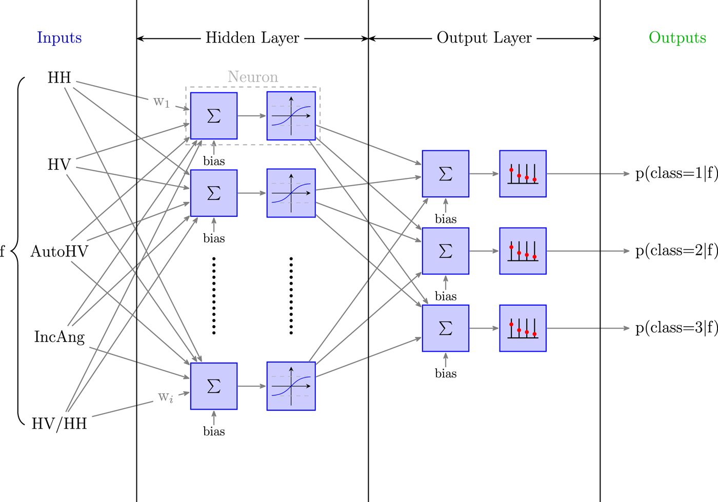
A feed-forward neural network with one hidden layer is used for the mapping between the image features and the different classes (Jain and others, Reference Jain, Mao and Mohiuddin1996). Artificial Neural Networks (ANN) are machine learning algorithms that need training data to obtain a network that can be applied to unknown data of the same kind to perform, for example a classification task. The architecture of the employed network is depicted in Figure 2. The network consists of three layers: the input layer, one hidden layer and an output layer where each layer has a number of neurons or nodes. The input layer has five neurons of pixel-wise image features, namely backscatter in HH and HV polarization, autocorrelation in HV polarization, incidence angle and HV/HH polarization ratio. No significant improvement in the classification was achieved by including HH autocorrelation. The hidden layer consists of four neurons where each neuron computes a weighted sum of the neurons of the input layer and evaluates the result with an activation function. A tangent sigmoid is used as the activation function in the hidden layer. The number of neurons in the hidden layer is determined such that good generalization is achieved while the number of neurons is kept as small as possible. We selected four hidden neurons as algorithm performance does not significantly increase with more neurons. The output layer consists of three neurons representing the targeted classes: water, thin ice/calm water and ice.
Schematic sketch of the utilized neural network.
The classes are coded in a 1-of-3 coding scheme where class k ∈ {1, 2, 3} is represented by a unit vector t with t k = 1 and t l≠k = 0 (Bishop, Reference Bishop2006). The activation function is a softmax function
 $$y_k = p(class = k \vert f) = \displaystyle{{\exp (a_k)} \over {\sum\nolimits_j {\exp (a_j)} }},$$
where the a k are the weighted sums of the outputs of the hidden layer and f the input feature vector. The output of the softmax function is equivalent to the probability p(class = k|f) of belonging to class k (Richard and Lippmann, Reference Richard and Lippmann1991).
Manually interpreted SAR images, where regions of interest (ROIs) were assigned to different ice classes, are used as targets for the training process. The classes have been identified by manual interpretation of backscatter characteristics, texture and spatial context of the SAR image scenes. Sea ice has a variety of backscatter intensities but usually shows features such as ridges, floe outlines or leads. Open water has much fewer features and the backscatter intensities are distributed more evenly even though wind or current induced patterns can be visible. Thin ice/calm water class comprises areas with very low backscatter intensities due to almost specular reflection and no textural features. From SAR images alone, thin ice and calm water cannot be distinguished unambiguously. It should be noted that SAR signatures of sea ice are very sensitive to small-scale properties of the ice, e.g. surface roughness and size and volume fraction of air bubbles within the ice. Thin ice could, therefore, also be represented by the ice class if the surface roughness is enhanced due to, for example rafting or frost flowers, resulting in increased backscatter intensities especially at C-band. A good overview of SAR signatures of open water and sea ice can be found, for example in Carsey (Reference Carsey1992) and Jackson and others (Reference Jackson and Apel2004).
The same number of training samples (4 000 000) has been used for the classes water and ice, while all defined samples of thin ice/calm water class have been considered due to their significantly smaller number (~60 000 samples for PALSAR-2 and 400 000 for Sentinel-1). These numbers also represent the relative occurrence of the classes within the scenes. The network uses scaled conjugate gradient backpropagation (Møller, Reference Møller1993) with cross-entropy as performance function for the training process. Ten networks have been trained for each frequency separately and the best performing one has been selected for deriving ice/water maps from the SAR images.
Data division
In total 24 ALOS-2 PALSAR-2 and 25 Sentinel-1 images are available for this study. Twelve images of each frequency are used for training of the neural networks. For those images, Regions of interest (ROIs) representing the three classes have been selected to set the training samples. All ROIs were selected by the same person to avoid biases in the manual interpretation. This dataset will be referred to as the training dataset.
The remaining images of the two sensors are used for the evaluation of the algorithm performance against ice charts and radiometer derived ice/water maps. This is termed as the evaluation dataset. Included in this set are six pairs of near-coincidental C- and L-band images, which are used to compare the algorithm outputs of the two frequencies.
The datasets are comprised of winter images from October to April with one summer scene from June 2015 used in the evaluation dataset. The division has been made such that images from the different months are represented in the test and evaluation dataset. For training, the same number of ascending and descending orbit images have been used.
Confusion matrix
The performances of the classifier are assessed using a confusion matrix, which compares the classification result to the training data (Stehman, Reference Stehman1997). The confusion matrix enables to identify the nature of error sources in the classification process.
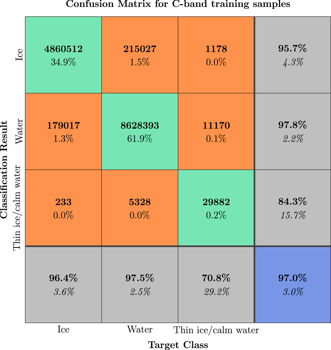
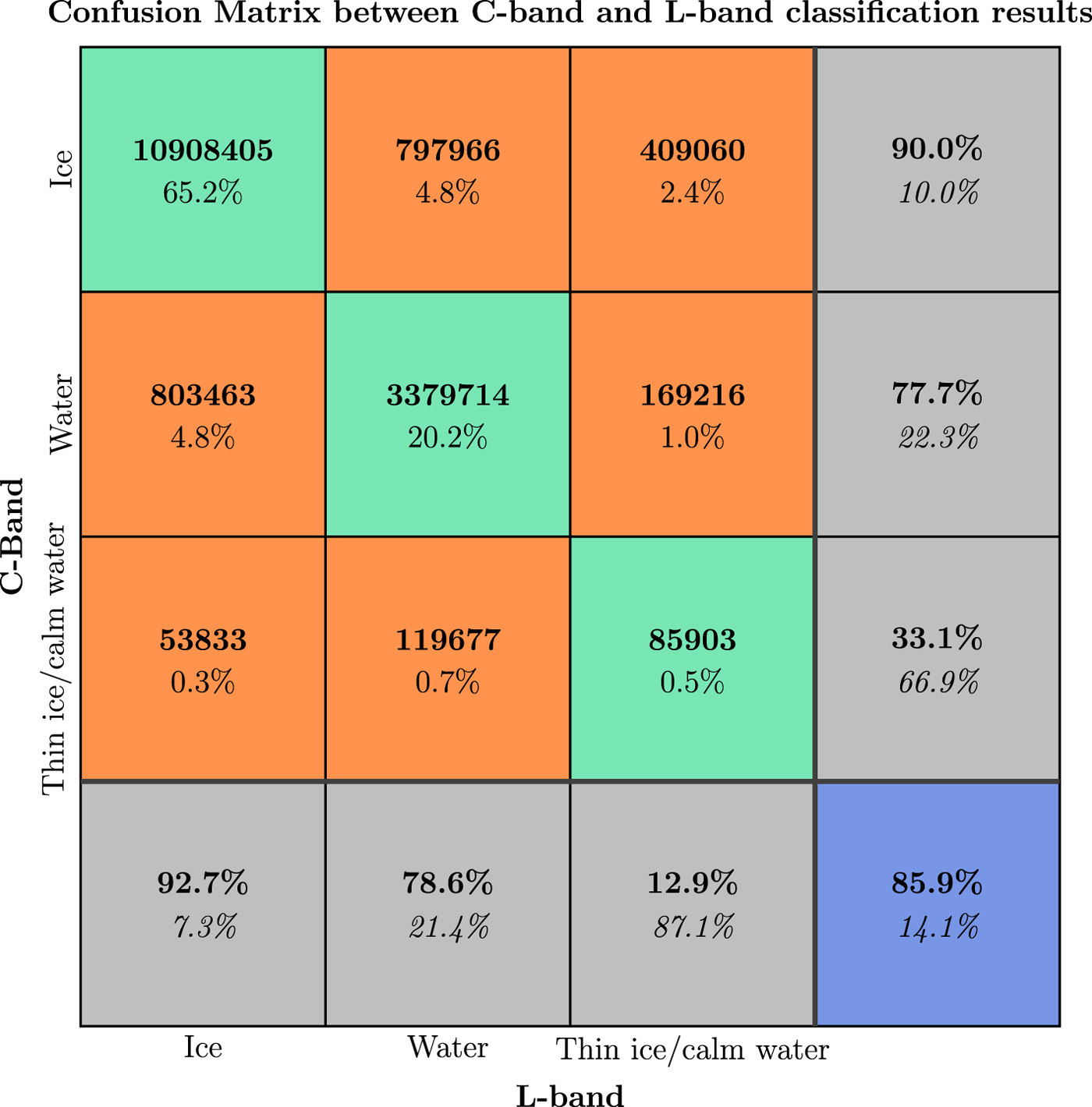
For the confusion matrices shown in this paper, we choose a representation where the classification results are denoted in the rows and the training samples in the columns. The main diagonal elements represent the number of correctly classified samples, highlighted in green, while off-diagonal elements show misclassified pixels, highlighted in orange. The last element of each column gives the accuracy, i.e. the fraction of correctly classified pixels with regard to the total number of pixels for this class in the training dataset. That is, the probability that the pixel is correctly classified. The last element of each row gives the reliability, i.e the fraction of pixels correctly classified with regard to the total number of pixels in this class. That is, the reliability gives the probability that a pixel classified into a class is indeed of this class. Reliability and accuracy are marked as grey in Figures 3, 4 and 6. The overall accuracy is the number of correctly classified samples divided by the total number of samples and is shown in blue.
Confusion matrix for classification results against training samples for C-band. Green and orange indicate correctly and incorrectly classified samples, respectively. Blue gives overall performance in percentage classified correctly (bold) and incorrectly (italic), while grey summarizes the accuracy (row) and reliability (column).
Confusion matrix for classification results against training samples for L-band. Green and orange indicate correctly and incorrectly classified samples, respectively. Blue gives overall performance in percentage classified correctly (bold) and incorrectly (italic), while grey summarizes the accuracy (row) and reliability (column).

RESULTS
Algorithm evaluation
Algorithm performance is first tested on all available training samples derived from the ROIs of the training dataset, which include the samples used for training of the network. Figures 3 and 4 present the confusion matrices between the classification results in the rows and the target training samples in the columns for C-band (Sentinel-1) and L-band (ALOS-2 PALSAR-2), respectively. For C-band an overall classification accuracy, i.e. percentage of total correctly classified samples, of 97% is achieved (Fig. 3), while for L-band the overall accuracy is 88.8% (Fig. 4).
For C-band accuracy (last row, Fig. 3) and reliability (last column) show values above 95% for ice and water classes and significantly lower values for the thin ice/calm water class. The smaller areas of thin ice/calm water class can be a reason for the lower separability of this class.
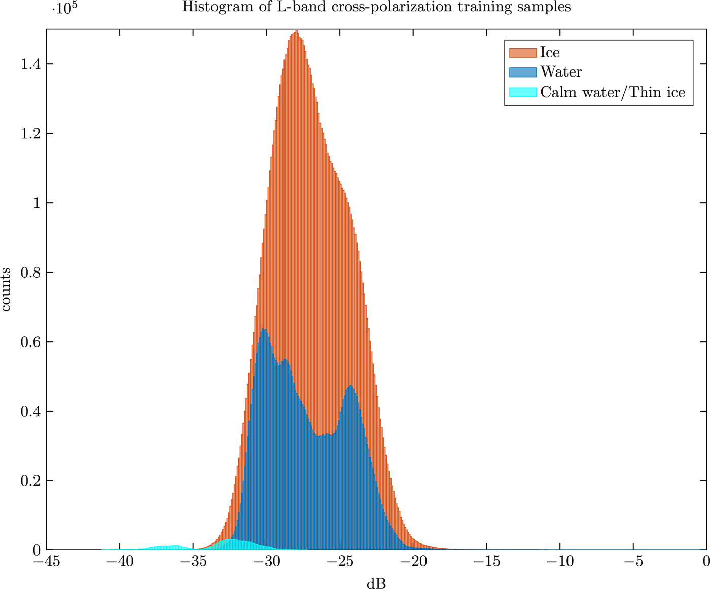
For L-band the accuracy is comparable for all classes, being slightly below 90% for ice and water and slightly above 90% for thin ice/calm water (Fig. 4). The reliability of the water class, that means whether a pixel classified as water actually is water, is however strongly reduced, mainly due to misclassification of ice into water. This indicates that underestimation of ice might occur in the final classification result. One reason could be the non-existent contrast between ice and water samples at cross-polarization. Figure 5 shows the distributions of cross-polarization backscatter values for all three classes. The overlap of ice and water samples reduces the separability between these two classes, especially when autocorrelation fails to discriminate these, for example where autocorrelation is low over sea ice. The reduced contrast is in line with observations over ice and water with ALOS PALSAR by Wakabayashi and others (Reference Wakabayashi, Mori and Nakamura2013).
Histogramm of all cross-polarization (HV) training samples at L-band.
The generalization capabilities of the algorithm, i.e. the ability of the networks to perform well on non-training data, are evaluated by applying the neural networks to the evaluation data-set and comparing the classification results against ice charts and ice/water maps derived from radiometer data. For this purpose the water and thin ice/calm water class have been combined into one single class, as no equivalent can be derived from the reference data. This choice introduces errors within the ice pack but reduces errors to a larger effect at calm water areas when compared with the reference data. The C-band and L-band classification results are resampled to the lower resolutions of the reference data to facilitate comparison. Ice/water maps from ice charts and radiometer ice concentration have been derived by setting a threshold of 15% ice concentration to distinguish ice and water. Radiometer data and downsampled ice charts show an agreement of 93.89% with a standard deviation of 2.48%. Largest differences occur at the ice edge. Ice charts are characterized by a loss of details due to the manual processing. Meanwhile, radiometer data are prone to larger errors in ice concentration estimation for low concentrations and thin ice (Spreen and others, Reference Spreen, Kaleschke and Heygster2008; Wiebe and others, Reference Wiebe, Heygster and Markus2009). Our method, which uses a concentration threshold to distinguish the classes, is hence affected by those errors. Ice drift seems to play a minor role for the deviations from the low-resolution reference data compared with the two aforementioned effects.
Ice charts are based on the latest available data, mainly SAR imagery when the ice chart is produced. For Sentinel-1, we can assume that the morning image has been considered. That implies a time difference of 7--15 hours to the imagery used in our study. The radiometer ice concentration maps use the latest available swath, which is recorded around noon for our area of interest, thus resulting in a few to 10 hours time difference. Ice drift in Fram Strait can reach values of up to 0.4 m/s and can thus be significant even in such time spans.
For C-band data, a mean accordance of 87.23% with a standard deviation 6.16% could be achieved in comparison with the ice charts and 89.33% with a standard deviation of 6.63% towards the AMSR2 radiometer data. At L-band a mean agreement of 84.17% with standard deviation of 6.86% is obtained in comparison with the ice charts and of 86.25% with a standard deviation 6.85% compared with the radiometer data. There is no significant preference of the C-band data in terms of better classification results when compared with the ice charts, which are mainly based on C-band imagery. The better agreement of our classification results with ice/water maps derived from radiometer data compared with the ice charts might be attributed to the loss of details at a lower resolution.
The main deviations between SAR derived ice maps and ice/water maps from ice charts and radiometer data occur in the marginal ice zone and at the thin ice/open water features within the ice pack. For ice charts, small features might have been omitted in the process of creating the chart when defining the outline of the polygons. The lower resolution reduces the effect of ice drift in between the acquisition of the data. Smaller features within the icepack are also visible in the radiometer data by a reduced ice concentration in those areas. But this reduction is not large enough to be picked up by the 15% threshold between ice and open water. This induces that some of the differences might not be attributed to actual misclassification but to different interpretations of the same situation in the datasets. A more detailed description of these effects will be given later on.
For one C-band scene (02.02.2016, scene centre: 79.5° N, 6.5° W) a severe misclassification over open water occurred, when high wind speeds (15 m/s) raised the cross-polarization return above the noise floor of the sensor and clear wind induced patterns could be seen. This situation has probably not been well reflected in the training data samples. One summer scene from 28.06.2015 was included in the evaluation dataset. In C-band, a more pronounced misclassification of ice into the water class can be observed within the pack ice while for L-band misclassification mostly occurred at the ice edge. This indicates that the algorithm needs to be tuned to accommodate the changing SAR signatures during the melting season.
Comparison of C-band and L-band
Six near-coincidental image pairs are included in the evaluation dataset. Figure 6 shows the confusion matrix between C- and L-band classification results of all near co-incidental image pairs. The diagonal matrix elements, highlighted in green, indicate matching classes while non-diagonal elements, highlighted in orange, show deviating classification results. The overall agreement, i.e. the class is the same in both images, is 85.9%. Accuracy and reliability are above 90% and thus indicate that ice is mostly ice in both frequencies. For water, the agreement between the two frequencies is significantly lower at 78.6%, which is also reflected in a lower reliability. The thin ice/open water class shows the least agreement. One reason for pixels classified as thin ice in L-band but as ice in C-band, is the lower separability of newly formed thin ice and young ice. L-bands larger wavelength on the one hand penetrates further into the ice and specular reflection occurs at the ice/water interface and on the other hand, is less sensitive to small-scale surface roughness from, for example frost flowers. Generally, differences between the two frequencies are more pronounced at the ice edge and these deviations are also reflected when the classification results are compared with the reference ice/water maps from ice charts and radiometer data.
Confusion matrix between classification results of all near-coincident C- and L-band image pairs. Green and orange indicate correctly and incorrectly classified samples, respectively. Blue gives overall performance in percentage classified correctly (bold) and incorrectly (italic), while grey summarizes the accuracy (row) and reliability (column).
The classification differences between the two frequencies are demonstrated in more detail on the basis of one example image pair from the 12.10.2015 but are characteristic for all the image pairs. The images were acquired 3 h apart, with L-band preceding the C-band acquisition. The images were taken on different orbital nodes, ascending for Sentinel-1 and descending for PALSAR-2. Wind speed was ~7 m s−1 according to ERA-Interim reanalysis data.
In Figure 7, a Sentinel-1 C-band and a PALSAR-2 L-band dual-polarization SAR scene from the 12.10.2015 are shown alongside the ice-water classification result. The red arrows indicate the flight direction and both satellites are right looking. Figures 7a and b show the HH and the HV backscatter intensity, respectively, in dB for Sentinel-1. In co-polarization the strong dependency on the incidence angle of the backscatter values over the open ocean can be seen while this is not evident over ice areas. The intensity decreases from near range on the left side of the image to far range on the right. In cross-polarization over low backscatter areas a characteristic repetitive pattern within the sub-swaths, additionally to the boundaries of the single scans, is visible. These stem from the Terrain Observation by Progressive Scans (TOPSAR) technique used for processing of the data and are not removed by the provided noise calibration (Miranda, Reference Miranda2015). Especially in the cross-polarization channel the boundary between sea ice and open water is clearly defined.
Example of SAR imagery and classification results from 12.10.2015. Upper panels from left to right show HH backscatter intensity, HV backscatter intensity and the classification result for the C-band Sentinel-1 case (Contains Copernicus Sentinel data 2015). Lower panels from left to right show the corresponding L-band data from ALOS-2 PALSAR-2 (copyright JAXA) and classification result. Red arrows indicate flight direction and time difference between the two images is ~3 h. The encircled area is discussed in the text.
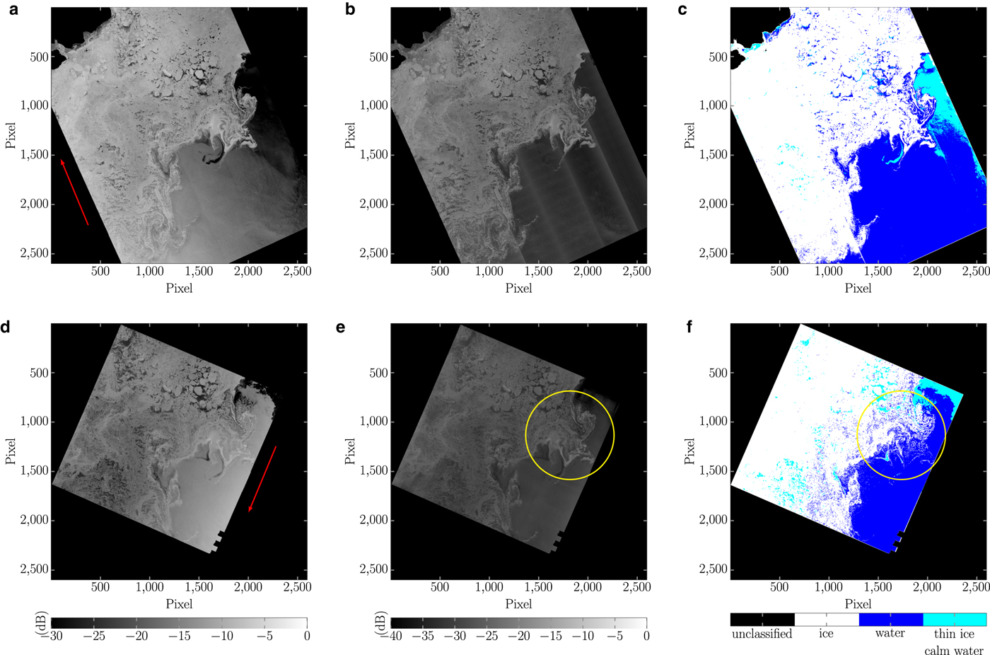
Figures 7d and e show the backscatter intensity in dB for the PALSAR-2 HH and HV channel, respectively. Generally, backscatter intensities are lower for L-band compared with C-band by ≈4.4 dB due to the longer wavelength. The open water at near range (right side of each image) shows a high backscatter decreasing slightly with incidence angle. The contrast between ice and water at cross-polarization is much lower compared with C-band. The quality for some scenes of the cross-polarization channel is severely degraded in low backscatter areas for the PALSAR-2 data though this effect is not pronounced in the selected scene. Striping and banding and a loss of resolution are observed in some but not all images and in non-regular patterns restricted to low backscatter areas. Compared with the C-band scene the same image features, for example ice edge and thin ice/open water areas in the pack ice can be visually identified.
In Figures 7c and f the results of the classification algorithm are presented, where ice is displayed white, open water blue and thin ice/calm water as cyan. The algorithm is able to pick up the features and complex outline of the ice edge and distinguish generally well between ice and open water areas for both frequencies. The yellow circle in Figures 7e and f outlines an area, where the algorithm for L-band shows less accuracy in classifying water and ice correctly. Smooth textures with relatively high backscatter are usually characteristic for near range open water and might be the reason for enhanced misclassification in this area.
The differences between the two frequencies are highlighted in Figure 8, where the C-band classification result is subtracted from the L-band result. For this plot the thin ice/calm water class is combined with the water class, to only distinguish two classes. Yellow shows water in L-band and ice in C-band, red indicates ice in L-band and water in C-band and blue depicts agreement. The area marked with a yellow circle in Figure 7e is clearly visible with yellow signature in Figure 8. Differences are pronounced for small scale features at the ice edge and in the ice pack. While ice drift played a minor role for misclassification with the reference data, it is not negligible for comparison of high resolution SAR derived ice/water classification maps. White outlined in Figure 8 are areas where ice drift has shifted features enough to disagree spatially and possibly also in their form and size. Indicative is the occurrence of both misclassification types, marked as red and yellow in the figure, in close proximity.
Difference of classification results between L- and C-band for the case 12.10.2015. Thin ice/calm water combined with water class for display. White outlined areas are explained in the text.
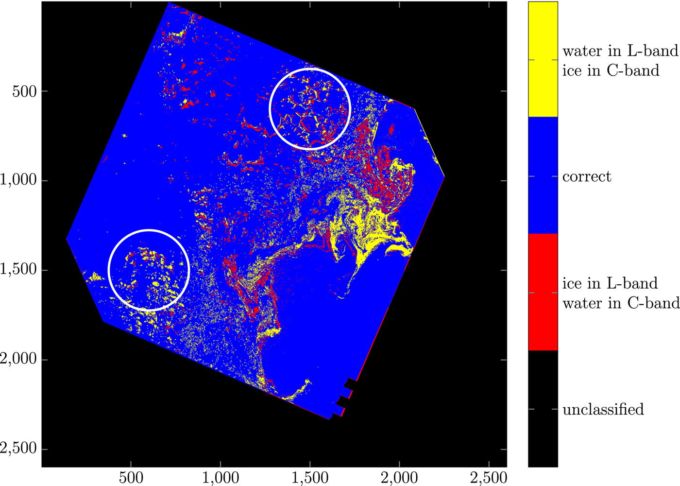
Figure 9 compares the ice charts and radiometer derived ice/water maps with the classification results of the algorithm. The black line in Figure 9a and the yellow line in Figure 9d denote the 15% concentration line, that distinguishes ice and water in the ice chart and radiometer data, respectively. For this comparison the thin ice/calm water class is combined with the water class for the SAR derived classification.
The upper panels show from left to right the ice chart and the difference to the classification result from Sentinel-1 and PALSAR-2 for 12.10.2015. The lower panels show from left to right the radiometer sea-ice concentration data and the difference to the classification results from Sentinel-1 and PALSAR-2. The black and yellow line in (a) and (d), respectively, show the 15% threshold used for ice/water delineation. Encircled areas A and B are discussed in the text.
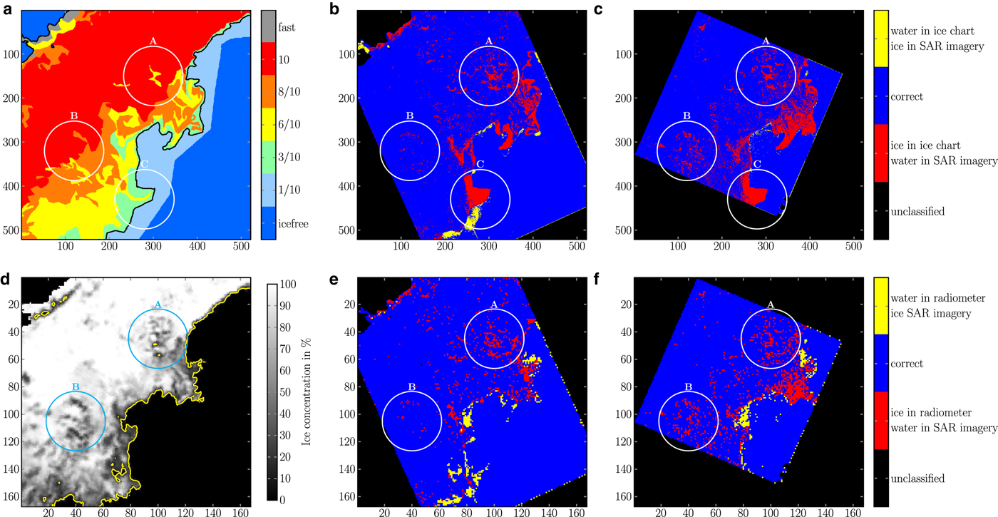
The largest deviations occur at the ice edge and small-scale features within the ice pack. The latter is highlighted in areas A and B in Figure 9. For these areas, a reduction of ice concentration is clearly visible in the radiometer data, while only area A shows lower ice concentration in the ice chart. The 15% threshold used for ice/water separation omit these features and they are, thus, visible as misclassification in the difference maps. These areas indicate that the differences between the SAR derived ice/water maps and ice charts and radiometer data highlight areas where thin or young ice is difficult to distinguish from open water. The texture of these areas is usually smooth and the backscatter intensities are lower than the surrounding ice, which are more common characteristics of open water than of ice.
Deviations at the ice edge between the SAR classification result and the ice charts mainly occur due to generalization when drawing the polygons outlining the different ice concentrations. Area C highlights a part of the ice edge where this effect is strongly pronounced (Fig. 9a–c). When comparing with the radiometer data, the differences at the ice edge can be attributed to the lower accuracy of ice concentration estimation at low ice concentrations and for thin ice areas affecting the accuracy of the selected 15% threshold (Spreen and others, Reference Spreen, Kaleschke and Heygster2008; Wiebe and others, Reference Wiebe, Heygster and Markus2009). The frequency differences in Figure 8, especially the area with predominantly yellow can also be identified by comparing Figures 9b with c and e with f, respectively.
CONCLUSIONS
The presented algorithm for ice/water classification of high resolution SAR imagery is able to produce accurate results for both C- and L-band compared with reference ice charts and ice concentration from radiometer data. Compared with ice/water classification results for Radarsat-2 C-band data from Leigh and others (Reference Leigh, Wang and Clausi2014) and Zakhvatkina and others (Reference Zakhvatkina, Korosov, Muckenhuber, Sandven and Babiker2017), our classification accuracy is slightly lower, <90% compared with 96% and 91%, respectively. The different scales and sources of the used images and validation data make a direct intercomparison difficult. Nevertheless, our algorithm is able to produce ice water maps capable of representing the complex outline of the ice-water edge as well as fine structures within the pack ice. Furthermore, the algorithm can be expanded by additional features to improve the classification result. This paper is to the best of our knowledge the first to investigate ice/water classification of L-band data from a satellite SAR sensor, thus no comparison can be made.
The ice edge is clearly outlined in C-band derived ice/water maps and a good separation between ice and open water is achieved. For one scene with high wind speeds, a severe degradation in ice water distinction was observed. Features within the pack ice, that most likely represent young ice, are attributed to open water because of their lower backscatter and smoother texture. At L-band, discrimination between ice and water is impeded in the marginal ice zone by reduced ice/water contrast at cross-polarization and an additional smoother texture caused by sub-resolution ice floes or pancake ice. Features within the icepack are mostly classified as thin ice/calm water, which reflects the actual ice situation. The differences between the two frequencies are in line with the characteristics of their wavelength with regard to the interaction with ice and open water.
Deviations between the two frequencies but also when compared with ice/water maps derived from ice charts and radiometer data occur mostly within the marginal ice zone and for small-scale features within the ice pack attributed to thin or young ice. While our algorithm preserves these features by classifying those as thin ice/calm water or water, the comparison ice maps omit those due to the threshold for binary ice/water classification. Technically thin and young ice should be classified as ice, but on the other hand, these areas provide valuable information, for example to determine the lead frequency or for navigation in ice-infested waters. Time difference between acquisitions plays a role for the direct comparison of ice/water from high-resolution SAR imagery but are of minor influence for comparison with the low-resolution reference data.
Though general features are well represented by our classification map, the algorithm leaves room for improvement especially in the marginal ice zone. In this area sub-resolution ice floes cause a smooth texture similar to water areas. Algorithm performance could be improved, for example by usage of additional texture features, i.e. derived from grey-level co-occurrence matrices, or different scales of texture features. The difference in interaction of the two frequencies with sea ice and open water, could be addressed by using different features in the training process of the neural networks. Furthermore, wind induced patters with high autocorrelation or increased backscatter intensities in cross-polarization over open water seem to be a challenge for the present algorithm. The inclusion of more training data representing high wind conditions could account for this issue. While Sentinel-1 data is freely available and a representative dataset can be obtained, access to ALOS-2 PALSAR-2 data is much more limited.
The image quality of the original SAR data is also an issue. The cross-polarization channel for Sentinel-1 is effected by its high noise floor and artefacts at subswath boarders can be visible in the classification result. ALOS-2 PALSAR-2 ScanSAR (level 1.5) images show degradation of image quality at low backscatter areas for some scenes in cross-polarization. The effects for Sentinel-1 are the same for all the images, but the degradation of the ALOS-2 PALSAR-2 is more random and not always pronounced. Howell and others (Reference Howell2018) report problems with the cross-polarization channel though they do not give further details. Here it should be kept in mind that ALOS-2 PALSAR-2 is designed for land observations.
C-band shows a more robust ice/water classification and is thus a better choice for this specific task. Nevertheless, ice water classification can be achieved with L-band data to increase temporal coverage. Furthermore, identification of thin ice areas within the ice pack is enhanced in L-band and thus could be of interest for applications in shipping and navigation. A combination of these two frequencies could possibly improve classification results. To date, the direct utilization of the two frequencies is obstructed by the time difference between acquisitions of different sensors.
ACKNOWLEDGMENTS
We thank the Swedish National Space Board for their research funding (contract dnr. 140/13). ALOS-2 PALSAR-2 data were provided by JAXA under the 4th ALOS RA, PI number 1331. We also thank the two anonymous reviewers for their constructive comments on the manuscript.


 Open access