Introduction

Predictions of the mechanical behaviour of ice in high-strain zones rely heavily on a knowledge of the expected type of fabric development in such a dynamic environment. Natural deformation of glaciers that is accomplished by deformation in ductile shear zones is accompanied by grain-size reduction involving intracrystalline slip with recovery to grain-size-insensitive dislocation creep to grain-size-sensitive diffusion creep (Reference Petrenko and WhitworthPetrenko and Whitworth, 1999). In most cases, the reduction in grain-size is achieved by dynamic recrystallization of larger grains that had a pre-existing crystallographic fabric. Dynamic recrystallization may alter the grain-size of materials during deformation by grain-boundary migration or formation of new high-angle boundaries (Reference PoirierPoirier, 1985). However, it has been suggested that initial fabrics influence the way dynamic recrystallization produces the final fabric (Reference Alley, Gow, Meese, Fitzpatrick, Waddington and BolzanAlley and others, 1997; Reference Piazolo and PasschierPiazolo and Passchier, 2002). As large strains are accumulated in these fine-grained regions, there is a question of whether there is any preservation of the initial fabrics and a misorientation distribution between neighbouring grains.

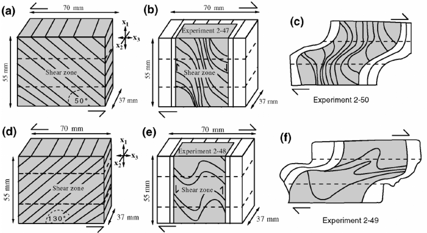
The interpretation of c-axis fabrics in shear zones is usually made with the assumption that there may be an inherited fabric component because we can identify folds in inherited layering, with the accommodation of strain in the microstructure being partitioned by the recrystallization processes. Many authors (e.g.Reference WilsonWilson,1981; Reference Lloyd, Law, Mainprice and WheelerLloyd and others, 1992; Reference Tison, Thorsteinsson, Lorrain and KipfstuhlTison and others, 1994; Reference Thorsteinsson, Kipfstuhl and MillerThorsteinsson and others, 1997) have interpreted such features as representing the persistence of original microstructural domains and lower-shear-strain features to higher shear strains. One cause of the lack of consensus regarding the way in which the role of adjacent grains is inherited from a precursor microstructure may be the lack of clear observational details. In this study, we undertake a two-stage experimental approach to deform a well-defined layered sample (Fig1). In the first stage we deform a sample with layers that are inclined to the bulk shortening and extension axes (Fig. 1a and d), as described by Reference Wilson and SimWilson and Sim (2002), to produce a buckled sample that contains a shear zone. The second stage is to rotate this sample 90° and add two ice wedges (Fig. 1b and e) and re-deform the sample under the same initial axial stress. The reoriented sample is therefore deformed from a mutually opposite direction to produce a variety of folded structures in the layering (Fig. 1c and f). In undertaking such a study we are attempting to replicate the fold development seen in ice sheets (Reference Alley, Gow, Meese, Fitzpatrick, Waddington and BolzanAlley and others, 1997) and glaciers (e.g. Reference Tison, Hubbard, Maltman, Hubbard and HambreyTison and Hubbard, 2000), particularly where a stratified ice mass rotates over a basement irregularity. Typically folds have been noted near the bedrock and are associated with single-maximum c-axis fabrics inclined to the normal of the foliation, or may be accompanied by multiple-maxima fabrics. In this paper, we attempt to illustrate the processes in the transition from an inherited fabric to the final fabric in a shear zone complicated by varying strain distributions in the folded layers. This work will also examine the effect of an initial fabric on the mechanical behaviour of the polycrystalline ice.

Fig. 1.

Experimental stages where initial samples (a, d) are deformed then rotated 90° (b, e) and re-deformed under the same physical conditions (c, f). (a) Stage 1 initial sample with layering inclined 50° to the x₂x₃plane (experiment 2-47). (b) Stage 2 where deformed sample 2-47 minus portion that was used to make vertical section was rotated 90° and inserted between ice wedges to have the same dimensions as in (a). (c) Sketch showing distribution of layers in vertical section (x₁x₃) at the completion of the stage 2 experiment 2-50 (d) Stage 1 with layering inclined 130° to the x₂x₃ plane (experiment 2-48). (e) Stage 2 where deformed sample was rotated 90° and re-deformed (experiment 2-49). (f) Sketch showing distribution of layering seen in a vertical section (x₁ x₃) at completion of experiment 2-49.

Experimental Procedure and Mechanical Behaviour

The tests described here were in a deformation apparatus and under conditions similar to those described by Li and others (1996) and were performed under both constant-load and constant-shear-strain conditions at –2°C. The test apparatus was located inside a freezer box, with the controls and recording system outside it, as described by Li and others (1996). The temperature was controlled by circulating silicon oil around a sample shielded by a film of aluminium foil. Thermistors were placed adjacent to the specimen and at selected sites in the silicon oil bath to record the temperature of the test. The temperature variation was never more than ±0.2°C during the month-long experiments. The ice-test sample was laboratory-prepared, comprising layers (-10 mm wide) of fine ice intergrown with elongate crystals, similar to that described by Wilson (1981). A sample measuring approximately 70 mm x 55 mm x 37 mm is frozen into two support boxes (as illustrated by Li and others, 1996), and the strain is not uniformly distributed, but localized to the centre of the sample (Fig. 2, zone 3). There are also transitional zones where the original layering is progressively rotated (Fig. 2, zone 2), and these are juxtaposed with relatively undeformed boundary zones (Fig. 2, zone 1).

Fig. 2.

Microstructure in x₁x₃ vertical sections (V) of deformed layered ice illustrated as axial-distribution (AVA) diagrams. The fine red lines illustrate the distribution of preserved layer boundaries. Dashed white lines enclose specific areas where c-axis concentrations were obtained. Shown at the bottom of the micrograph is the shortening ("¹) that is applied parallel to the x ¹ axis (Fig. 1) and the shear strain (γ) recorded across the shear zone. (a) The colour code shows the relative azimuth and plunge of the pixel distribution across the thin section that relates to the c-axis orientation. (b) Experiment 2- 47 after stage 1 deformation where the greatest degree of recrystallization and layer rotation occurs within a ∽10 mm wide zone that transects the sample (zone 3), bounded by two transitional regions (zone 2), with zone 1 containing a high proportion of undeformed host grains. (c) Experiment 2-50 after stage 2 deformation. (d) Experiments 2-48/2-49 after stage 2 deformation. Layers 1 and 2 are preserved from experiment 2-48.

Creep curves for each test are shown in Figure 3. The creep curves are plots of octahedral strain rate as a function of octahedral strain and demonstrate that, under these test conditions, the octahedral strain rates for experiments 2-47, 2-49 and 2-50 (i.e. the strain to the minimum) are very similar. The creep curve for 2-48, by contrast, is not a simple decrease in strain rate but preserves an inflection that may reflect an initial resistance to buckling occurring in the layering that was inclined perpendicular to the shearing direction (experiment 2-48; Fig. 1d). Experiments 2-47 and 2-48 reach a minimum (at ~ 1 x 10^–7 s–¹) after 1 % octahedral shear strain, and beyond this point all of the curves for stage 1 exhibit strainrate increases to a greater tertiary strain rate and follow similar paths (Fig. 3). All of the re-deformed samples (experiments 2-49 and 2-50) reach minimum strain rates of ~4 x 10^–7 s–¹, but beyond this point the strain rate increases and then decreases at octahedral shear strains of ~ 8 % before undergoing a secondary increase (curves for 2-49 and 2-50; Fig. 3). The creep curve for experiment 2-49 has a greater tertiary strain rate than the other samples and suggests that the initial pattern of crystal-orientation fabrics and rate of rotation of the inherited layering govern the shear strain rate.

Fig. 3.

Creep curves for samples experimentally deformed at –2°C in combined compression and shear with a compressive stress of 0.22 MPa and shear stress of 0.4 MPa. (a) Creep curves for deformed (stage 1; experiment 2-48 with initial layering inclined 130° to the x₂x₃ plane) and re-deformed sample (stage 2; experiment 2-49 where the stage 1 sample is rotated 90). (b) Creep curves for deformed (stage 1; experiment 2-47 with initial layering inclined 50° to the x₂x₃ plane) and re-deformed sample (stage 2; experiment 2-50 where the stage 1 sample is rotated 90^˚).

Orientation of caxes was obtained using the fabric analysis apparatus illustrated in Figure 4 and using the apparatus described by Reference Russell-Head and WilsonRussell-Head and Wilson (2001). The analysis process works in two stages: (1) The analytical instrument scans the thin section and collects and processes image data. (2) The section data acquired from the analytical instrument are loaded into a separate analysis software (called INVESTIGATOR) that allows the operator to examine individual crystallographic variation across individual grains. Unlike traditional texture analysis, the information allows considerable interactive data processing, using INVESTIGATOR, as the link between microstructure and individual c-axis orientations.

Fig. 4.

Sketch of fabric analyzer. The computer-controlled fabric analyzer uses five imaging axes to simultaneously crossed-polar images of the thin-section material. The polarizers and retarder plate are directly mounted on high-resolution motors, and high-intensity light-emitting diodes provide the light source. The real-time analysis of images using the INVESTIGATOR software uses images obtained from the five cameras as the polars are rotated, with and without the retarder provides the information necessary to reconstruct the individual c-axis orientation for each pixel in the section image.

Therefore the new system for fabric analysis separates the instrument from the analysis. The instrument (Fig. 4) automatically scans a thin section and collects sets of tiled images that represent stepped rotations of crossed polars in three oblique directions through the section. The lower polarizer has a retarder plate that resolves the plane containing the c axis of the ice crystal. The intersection of the planes from the three oblique views provides the c-axis direction. Theanalysis software provides user feedback on the position of the three planes and their intersections at each pixel in the thin-section image. It is easy to choose where to make a determination and to get immediate indication of the quality of the determination.This technique is at least as reliable as the standard Rigsby stage method. The next version of the instrument is expected to yield higher accuracy, which will be independently tested by comparison with the electron backscatter technique using a quartz thin section.

The microstructural images acquired were typically on the order of 2000 x 2000 pixels that were decomposed and reprocessed as axial-distribution diagrams or AVA diagrams (Achsenverteilungsanalysis) or as scatter diagrams of individual grain c-axis orientation plotted on an equal-area stereographic net. A standard colour code (Fig. 2a) was used to identify the c-axis directions as azimuths and dips in the micrographs. In this scheme, north-trending axes are in blue, east-trending axes are in orange, axes normal to the plane of the thin section are in black and gradational shades represent angular differences between neighbouring pixels. A change in colour intensity to the centre of the colour circle (black) corresponds to c axes increasing in plunge from horizontal, on the periphery, to vertical at the centre of the net. This is an easy method of measuring ice grain orientations, and large datasets can be collected quickly (e.g. in this study 450 grains were measured and analyzed in 2 hours). The c-axis fabrics were measured in two planes, one horizontal section (H) oriented parallel to the shear zone and parallel to the direction of shear, and a vertical section (V) perpendicular to the foliation and parallel to the direction of shear.

Textural and Microstructural Evolution

At the termination of the stage 1 deformation, the AVA diagram illustrates a central high-strain zone (zone 3, Fig. 2b) where there is a concentration of grains with c axes oriented sub-parallel to the shortening direction. This is clearly seen from the concentration of blue grains in Figure 2b, that corresponds to the orientation spread seen in the colour wheel (Fig. 2a). In the least deformed zones (zone 1; Fig. 5a), there is a retention of the random c-axis pattern of the starting material. Elements of this pattern are also observed in measurements obtained in the intermediate strain zone (zone 2; Fig. 5b). However, in the higher-strained area (zone 3; Fig. 5c), there are two asymmetric concentrations of c axes relative to the compression axis with a strong single maximum, rotated with the sense of shear. This pattern of preferred orientation has been reproduced in duplicate experiments (Fig. 6a), where the sample was not required for re-deformation. Here the c-axis pattern measured in horizontal sections, that parallel the shear zones (Fig. 6b; fabric diagram 2-43 H, zone 3), displays strong concentrations of c axes that lie at high angles to the central shear zone (Fig.5c). There are two asymmetric concentrations of c axes relative to the compression axis with a strong single maximum, rotated in the direction of the sense of shear.

Fig. 5.

Orientation relationships in a vertical section through the deformed sample 2-47 (Fig 2b) seen after stage 1, but prior to the sample being rotated 90° and re-deformed (stage 2). (a–c) Lower-hemisphere equal-area projection showing the distributions of c axes, neighbour-pair and random-pair mis orientation distributions measured from zones 1 (a), 2 (b) and 3 (c) that are illustrated in Figure 2b.

The fabric transition into the zone of higher shear strain is very rapid. This is well illustrated on the scale of the total sample or within individual zones. Randomly oriented grains in zone 1 (Fig. 5a) are rapidly transformed into the two-maxima pattern seen in zones 2 and 3 (Fig. 5b and c). This is well highlighted in any individual layers (e.g. zones 2A, 2AA and 3A; Fig. 2b) where a small population of grains exhibit the same pattern (Fig. 7a). This central region of the sample with its strong crystal fabrics was then rotated 90° (Fig. 1b and e) so that the asymmetric maxima were lying east–west (e.g. Fig. 8d), rather than north–south, at the commencement of the stage 2 deformation (Fig. 1b and e). The reason for undertaking this rotation is to simulate the situation in a glacier where layering is rotated as the ice mass passes over basement riser as reported by Reference Tison, Thorsteinsson, Lorrain and KipfstuhlTison and others (1994).

Fig. 6.

Lower-hemisphere equal-area projections showing the distributions of c axes, neighbour-pair and random-pair misorientation distributions measured in vertical (V) and horizontal (H) sections within zone 3 of deformed sample 2-43. Shortening (ε¹ = 12.1%) and shear strain (γ =2.11) are comparable to experiments 2-47 and 2-49; in the latter two tests it was not possible to make horizontal sections.

Fig. 7.

Stereonets showing the distributions of c axes in vertical sections through experiments 2-47, 2-50 and 2-49. The azimuths correspond to the colour code (Fig. 2a), with the zero or north point parallel to the compression axis. (a) Experiment 2-47 showing c-axis distributions within individual layers, namely zones 2A, 3A and 2AA (for location see Fig. 2b). (b) Experiment 2-50 showing total scatter diagrams in zones 1–3 and c-axis distributions within individual layers, namely zones 1A and B, 2A and B, 3A and B (for locations see Fig. 2c). (c) Experiment 2-49 showing total scatter diagrams in zones 1–3 and c-axis distributions within layers 1 and 2, and the overlapping area E (for location see Fig. 2d). The measurements in areas A–D are from different regions of relatively undeformed zone 1.

Fig. 8.

Distribution of misorientation angles between adjacent ice grains and corresponding c-axis distributions. (a) The neighbour-pair misorientation distribution in the starting material. Misorientations below 10 are designated sub-grains. (b) Lower-hemisphere equal-area projection showing the distributions of caxes in the starting material. (c, d) Distribution of misorientation angles between adjacent ice grains and corresponding c-axis distributions in stage 1 from experiment 2-47 and recorded in zone 3. (e, f) Distribution of misorientation angles between adjacent ice grains and corresponding c-axis distributions in stage 2 from experiment 2-50 and recorded in area C, zones 1A and 1B.

At the conclusion of stage 2 deformation, the c-axis patterns seen across the samples show quite considerable variations in localized areas (Fig. 7b and c). In the least deformed zones (zone 1; Fig. 7b and c) there is a near-random c-axis pattern that reflects in part the inherited fabric; this also has contributions from the starting material used to enclose the stage 1 sample (e.g. Fig. 2c, areas A and B; Fig. 2d, area A). In zones 1A, 1B and area C (Fig. 2c), however, there are elements of an inherited east–west concentration of c axes, from the zone 3 pattern developed in stage 1 (Fig. 7b, zones 1A and 1B). The transitional zone 2 also incorporates part of this east–west inherited fabric, but has superimposed on it a strong asymmetric sub-maximum that lies oblique to the plane of shearing and direction of shortening (Fig.7b, zones 2, 2A and 2B), whereas, in the highly sheared portion of the samples (e.g. Fig. 7b, zones 3,3A,3B; Fig. 7c, zone 3), there is one strong maximum and sub-maximum that are asymmetric with respect to the shear zone boundary. This central zone preserves no evidence of the pre-existing fabrics (e.g. Fig. 7c, area E). By analogy with numerical fabric studies (e.g. Reference Van der Veen and WhillansVan der Veen and Whillans, 1994; Reference Ximenis, Calvet, Garcia, Casas, Sabat, Maltman, Hubbard and HambreyZhang and Reference Wilson and ZhangWilson, 1997), this asymmetrical c-axis fabric distribution is considered to be indicative of non-coaxial (approximately simple shear) strain histories.

Depending on the initial layer orientation with respect to the direction of shear, two different patterns of layer folding were produced as a result of stage 1 deformation, and these produce differences in the creep behaviour (Fig. 3). The initial yielding of the layered ice, where the layering is inclined with the direction of shear (Fig. 1b; experiment 2-47), produces sigmoidal-shaped layering consistent with the sense of shear (Fig.1a; see also Reference Wilson and SimWilson and Sim, 2002). Where the initial layering was inclined to the shearing direction (Fig.1d; experiment 2-48), the layering is folded into a series of open buckles (Fig.1e). These layers are defined by the preservation of air bubbles along the original layer boundaries. The grain microstructure that is associated with this deformation is characterized by a serrated interlocking grain structure, and throughout the whole sample there is a noticeable absence of undulose extinction within any grain (Fig. 2b). Accompanying the strain in the shear zones (zone 3), there was a subtle reduction in grain-size (Fig. 2b), which is comparable with the more extensive set of results described by Reference Wilson and SimWilson and Sim (2002).

After the stage 2 deformation, the original sigmoidal pattern seen in experiment 2-47 is refolded (Fig. 1c). However, the preservation of the original layering in the shear zones is difficult to recognize in thin sections (60 μm thick) but can be ascertained in thicker slabs cut from the sample (120μm thick). The grain microstructure in the high-strain zone (Fig. 2c, zone 3) is dominated by fine recrystallized grains (diameter 1–3 mm) in the re-deformed area (Fig. 2c, zones 3A and 3B); here there is a prominent two-maxima c-axis crystallographic fabric (Fig.9b). The transitional lower-strained areas (e.g. Fig. 2c, zones 2A and 2B) have a greater grain-size (2.5–10 mm) and a greater distribution of c axes lying in the east–west quadrant (Fig. 9e) that may reflect an inherited east–west component from stage 1.

Fig. 9.

Grain misorientation distribution between adjacent grains and corresponding c-axis distributions in experiment 2-50 from areas of high strain (zones 3A and 3B; Fig 2c) and intermediate strain (zones 2 A and 2B; Fig 2c). (a, d) The neighbour-pair misorientation distributions. (b, e) The total c-axis distributions in zones 3A, 3B, 2A and 2B (Fig 2c). (c, f) The c axes corresponding to the grains that belong to misorientation subsets: intermediate-angle (10–25°), high-angle (50–65°) and very high-angle boundaries (120–150°).

Where a set of original upright folds (Fig. 1e) are sheared and flattened (Fig. 1f), a complicated set of disharmonic fold structures (Reference Van der Pluijm and MarshakVan der Pluijm and Marshak,1997) are produced that are asymmetric in the direction of shear (Fig. 2d). The pre-existing layering is difficult to recognize in thin section because of extensive grain growth, with variable grain-sizes (2–7 mm), in zones 2 and 3, and the corresponding c-axis fabrics in these areas all exhibit evidence of a two-maxima pattern (Fig.7c, zones 2 and 3). There is a complete removal of evidence of the earlier east–west-trending caxes in layers 1 and 2 (Fig. 7c), with all grains contributing to the two-maximapattern seen in the total plot for zone 2 (Fig.7c). This is in marked contrast to the lowest-strained regions (Fig. 7c, zone 1) where there are smaller grain-sizes ∽3mm in area B, 2–5mm in area C and 5–6mm in area D (Fig. 2d). These lower-strained areas preserve elements of the pre-existing east–west-trending c-axis fabric and retain the original grain-size (areas B and C; Fig. 2d) or have experienced apparent grain growth (area D; Fig. 2d).

Misorientation Distribution Data

Misorientation distribution data provide more information about intra-grain processes in the development of the c-axis orientation patterns (Reference Wheeler, Prior, Jiang, Spiess and TrimbyWheeler and others, 2001) and may help us to understand texture-forming processes and deformation mechanisms. The normal method is to select the minimum misorientation angle and its corresponding rotation axis (Reference Alley, Gow and MeeseAlley and others, 1995). As pointed out by Reference Wheeler, Prior, Jiang, Spiess and TrimbyWheeler and others (2001), there is generally no physical significanceto this convention, and it does not necessarily mean that two grains are misoriented because they have actually rotated around a chosen axis. In this paper, any set of grain pairs is used to calculate a set of misorientation angles using the method described by Reference Wheeler, Prior, Jiang, Spiess and TrimbyWheeler and others (2001). The misorientation-angle distribution of every grain is related to every other grain and represented graphically by a histogram of misorientation angles or by a cumulative frequency curve. Our database for misorientation analyses is the collection of c-axis measurements of crystallographic orientations. These data allow us to perform two kinds of misorientation analysis (Fig. 5, 6, 8 and 9): (1) a neighbour-pair misorientation calculated from two c-axis orientation measurements, either side of a boundary between neighbouring grains, and (2) a random-pair misorientation calculated from the orientations of grain pairs that are not necessarily in physical contact (Reference Fliervoet, Drury and ChopraFliervoet and others, 1999). The dataset size is, in the case of neighbour-pair misorientation distribution, related to the number of measured neighbouring grain pairs. In the case of the random-pair misorientation distribution, the measured c axes of the neighbouring grain pairs are randomly paired. It is expected that important information about grain boundaries can be detected by comparing the misorientation distributions. In the following, we present the results from grain misorientation analyses performed on zones representing the transition from low to higher strains.

In the starting material the neighbour-pair misorientation distribution appears to be either essentially random (Fig. 5a) with no distinct population groupings, or a broad girdle (Fig. 8a) that appears to correspond to crossed girdle distribution (Fig. 8b). After stage 1 of the deformation history, the high-strain zone in the centre of the sample has a neighbour-pair misorientation c-axis distribution that is non-random, characterized by a peak at 10–30°, a sub-peak centred at 50–65° and a broad peak at 120–150° (Fig. 5c and 8c). The neighbour-pair misorientation distribution is very similar to the random-pair misorientation distribution and suggests that grains are not influenced by their neighbours (Fig. 6). These non-random fabrics were then rotated and re-deformed in order to see what strain regime would preserve these fabrics.

Figure 8 shows the significant changes that can occur in the c-axis pattern and the neighbour-pair misorientation distribution from prior to stage 1 deformation (Fig. 8a and b) at the onset of stage 2 deformation (Fig. 8c and d) and in an area that did not undergo shearing (Fig. 8e and f). Prior to stage 2 deformation, the pattern would have been east–west concentrations of c axes (Fig. 8d), due to rotation of the sample, in grains with diameters of 2–4 mm (Fig. 2b, zone 3). Remnants of this pattern are still seen, but there is the initiation of new grains with steep plunging c axes that randomizes the previous fabric (Fig. 8f) and substantial grain growth (e.g. zones 1A, 1B and area C in Fig. 2c; areas B, C and D in Fig. 2d). This produces a reasonably flat distribution of neighbour-pair misorientations with sub-peaks at 15°, 60°, 115° and 130–140° (Fig. 8e). These sub-peaks are not strong and do not match up with the misorientation angles observed after the stage 1 deformation (Fig. 5b and c). Although these areas were not experiencing substantial deviatoric stresses, there was sufficient stress to promote grain growth with the removal of some of the strongly oriented grains (Fig. 8d), and initiate new grains with orientation fabrics. This may reflect migration recrystallization in a constrained environment (Fig. 8f).

In contrast to this random pattern, areas that experienced any component of shear strain (zones 2 and 3) exhibit no evidence of inherited c-axis component, namely the preexisting east–west-trending fabrics (e.g. Fig. 9). Neighbourpair misorientations suggest there are distinct subsets of preferred c-axis misorientation angles, namely intermediateangle (10–25°), high-angle (60–65°) and very high-angle (120–150°), that are identified in the higher-strained (Fig. 9a) and lower-strained areas (Fig. 9b). As illustrated by Reference Wheeler, Prior, Jiang, Spiess and TrimbyWheeler and others (2001), the neighbour-pair misorientation distribution depends on which grain pairs are neighbours. This is illustrated in Figure 9 where the particular subsets (Fig. 9c and f) that contribute to the final c-axis preferred orientation (Fig. 9b and e) are separated out. It is clearly seen that the strongly clustered set of orientations contributing to the strongest concentration of c axes belongs to the intermediate angles 10–25°.

Discussion

Conclusions

1. 1. Advances in optical imaging techniques that allow the preparation of axial-distribution (AVA) diagrams, combined with computer-aided measurements, have been used for the preparation of individual c-axis orientation data. This has allowed routine analysis of individual grain-orientation determinations to be undertaken across a set of experimentally deformed samples of layered ice. Unlike traditional texture analysis, the information allows considerable interactive data processing with a strong link between microstructure and fabric data.

2. 2. These experiments suggest that at small strains there is a rapid change in c-axis crystallographic fabric through a process of dynamic recrystallization. Two dominant clusterings (point maxima) of c axes are present in any sample experiencing shear strains of γ ≥ 0.7: a dominant c-axis point maximum lying approximately 5° from the pole to the bulk shear plane and in the direction of shear, with a secondary maximum 45° to the shear plane.

3. 3. Pre-existing fabrics can be destroyed or modified by migration recrystallization that occurs in regions of lower differential stress and is accompanied by extensive grain-boundary migration (e.g. the transition from Fig. 8d to Fig. 8f). However, at sufficiently small strains, there is a switch from grain-boundary migration processes that can be considered as migration recrystallization, to the grain-size-sensitive mechanisms involving dynamic recrystallization.

4. 4. Individual c-axis orientation determinations across grain boundaries have been analyzed as neighbour-pair and random-pair misorientation distributions. The misorientation axes and crystallographic orientations indicate that there are distinct sets, which imply that adjacent grains have physically interacted to create special boundary relationships in the recrystallized aggregate.

5. 5. The grain-sizes of the recrystallized ice are quite coarse (≥1mm), and subgrains are not recognized optically; similarly, the absence of low-angle misorientations between c axes suggests that subgrain rotation is minimal or is obliterated by the dynamic recrystallization processes.