





1. Introduction
Semantic textual similarity (STS) measures the semantic equivalence between two sentences. This makes STS a crucial preliminary step in many NLP tasks, such as intelligent question answering, machine translation (MT), and automatic summarisation. For intelligent question-answering tasks, all candidate answers are ranked according to sentence similarity to a given question (Wang et al. (Reference Wang, Smith and Mitamura2007); Yang et al. (Reference Yang, Yih and Meek2015)). In MT, sentence similarity is used to judge whether two sentences have the same meaning (Yin and Schütze (Reference Yin and Schütze2015); He et al. (Reference He, Wieting, Gimpel, Rao and Lin2016); Santos et al. (Reference Santos, Alves and Oliveira2020)).
Existing work on STS can be broadly divided into two categories: lexicon-based and semantic-based. Lexicon-based approaches (Richardson and Smeaton (Reference Richardson and Smeaton1995); Niwattanakul et al. (2013); Opitz et al. (Reference Opitz, Daza and Frank2021); Wang and Yu (Reference Wang and Yu2023)) calculate the correlation between the character streams of two sentences being compared, which can be applied at the level of characters or words. The major core of semantic-based approaches is text representation. Current text representation approaches are mostly based on two models: sequence models and structured models. Regarding the studies on sequence models, Pagliardini et al. (Reference Pagliardini, Gupta and Jaggi2018) and Le and Mikolov (Reference Le and Mikolov2014) proposed Sent2vec and Doc2Vec to calculate sentence similarity, which use pre-trained word/sentence embeddings directly for the similarity task without training a neural network model on them. He et al. (Reference He, Gimpel and Lin2015) proposed an elaborate convolutional network (ConvNet) variant which infers sentence similarity by extracting features at multiple levels of granularity and using multiple types of pooling. Mueller and Thyagarajan (Reference Mueller and Thyagarajan2016) proposed a siamese recurrent neural networks, which use two identical long short-term memory (LSTM) networks to project zero-padded word embeddings of a sentence to fixed-sized 50-dimensional vectors using Manhattan distance as the similarity function between 2 sub-networks. Tharindu et al. (Reference Tharindu, Orasan and Mitkov2019) extended the siamese recurrent neural networks and used thesaurus-based augmentation (Miller, Reference Miller1992) to add 10,022 additional training examples. The siamese recurrent neural networks acquire excellent results. Bidirectional Encoder Representations from Transformers (BERT) (Devlin et al. Reference Devlin, Chang, Lee and Toutanova2019) is a pre-trained transformer network (Vaswani et al. Reference Vaswani, Shazeer, Parmar, Uszkoreit, Jones, Gomez, Kaiser and Polosukhin2017), which set new state-of-the-art results for various NLP tasks, including question answering, sentence classification, and sentence-pair regression. BERT and RoBERTa (Liu et al. Reference Liu, Ott, Goyal, Du, Joshi, Chen, Levy, Lewis, Zettlemoyer and Stoyanov2019) have set a new state-of-the-art performance on sentence-pair regression tasks like STS. Reimers and Gurevych (Reference Reimers and Gurevych2019) proposed Sentence-BERT (SBERT), a modification of the pre-trained BERT network, and it uses siamese and triplet network structures to derive semantically meaningful sentence representations. Based on the BERT model, Gao et al. (Reference Gao, Yao and Chen2021) proposed SimCSE, a simple contrastive sentence embedding framework, which can produce superior sentence embeddings. Various contrastive learning-based approaches (Chuang et al. Reference Chuang, Dangovski, Luo, Zhang, Chang, Soljacic, Li, Yih, Kim and Glass2022) rely on two main components, data augmentation and an instance-level contrastive loss. However, the discrete nature of the text makes it challenging to establish universal rules for effective text augmentation generation. Zhang et al. Reference Zhang, Xiao, Zhu, Ma and Arnold2022 tackle the challenge by presenting a neighbourhood-guided virtual augmentation strategy to support contrastive learning. As it is widely acknowledged that structural information is vital for NLP (Nguyen et al. (Reference Nguyen, Joty, Hoi and Socher2019); Zhang et al. (Reference Zhang, Wu, Zhou, Duan, Zhao and Wang2020)), there is an increasing interest in improving text representation by using syntactic information.
In order to use sentence structure information, Richard et al. (Reference Richard, Perelygin, Wu, Chuang, Manning, Ng and Potts2013) proposed to use a recurrent neural network to construct a text representation. This method applied a pre-specified parse tree to the recurrent neural network (RNN) to construct a structured representation. Tai et al. (Reference Tai, Socher and Manning2015) proposed a generalisation of the standard LSTM architecture to tree-structured and showed its superiority for representing sentence meaning over a sequential. Most of these works enhanced pre-trained language model (LM) by adding syntax-driven attention components to the transformer (Li et al. (Reference Li, Zhou, Li, Xu and Cao2021); Xu et al. (Reference Xu, Guo, Tang, Su, Shou, Gong, Zhong, Quan, Duan and Jiang2021); Bai et al. (Reference Bai, Wang, Chen, Yang, Bai, Yu and Tong2021)). They used the added components to produce a syntax-aware representation and inject this additional representation into the origin alone from the vanilla transformer so as to get a final syntax-enhanced representation. There are also some efforts on incorporating syntax-related objectives into the pre-training stage, such as syntax head prediction (Wang et al. Reference Wang, Tang, Duan, Wei, Huang, Cao, Jiang and Zhou2021) and dependency distance prediction (Xu et al. Reference Xu, Guo, Tang, Su, Shou, Gong, Zhong, Quan, Duan and Jiang2021). Zhang et al. (Reference Zhang, Xiao, Zhu, Ma and Arnold2022) proposed the syntax-guided contrastive language model (SynCLM). Based on contrastive learning, SynCLM uses syntactic information to create contrastive positive and negative examples and uses them to help the pre-trained LM to learn rich syntactic knowledge. Yet, there are few available resources for treebank annotations, and the results of existing grammatical analysis models are not very satisfactory.
In the absence of corpus resources, reinforcement learning is introduced to solve problems to a certain degree (Yogatama et al. (Reference Yogatama, Blunsom, Dyer, Grefenstette and Ling2017); Feng et al. (Reference Feng, Zhang, Hao and Chen2017)). Zhang et al. (Reference Zhang, Huang and Zhao2018) proposed a reinforcement learning (RL) method to build structured sentence representations by identifying task-relevant structures without explicit structure annotations. The frame structure of the sentence can promote the understanding of the overall structure of the sentence, but the sentence components can better reflect the semantic information of the sentence. However, the above models use reinforcement learning to learn sentence structures and build sentence representations with structures. They only refer to the sentence structure at the phrase level, without indicating the role of words in the sentence.
In this paper, we propose a skeleton-based reinforcement learning approach to increase similarity calculation accuracy. Skeleton grammar is essentially a selected subset of dependency grammar, which not only constructs the sentence structure but also indicates the function of each word in the sentence. The approach consists of three components: policy network (PNet), sentence representation model (SRM), and similarity calculation model (SCM). First, the skeleton words are identified through the policy network. Then the skeleton words are delivered to the SRM. According to the skeleton words, the sentence representation is constructed in the framework of parallel networks by designing two sentence representation models: CC-LSTM and AS-LSTM. CC-LSTM builds the sentence representation by constrained word context, and it is thought the relationship between the front word and the back word of the skeleton word is not close, so the skeleton word will be used as the boundary of the context. AS-LSTM first identifies the skeleton word of the sentence and then constructs the skeleton representation of the current skeleton word through the qualifier of the skeleton word. AS-LSTM not only highlights the primary information of the sentence but also retains the secondary information.
2. Related work
2.1 Application of reinforcement learning in NLP tasks
RL (Gu et al. Reference Gu, Shen, Shen, Shang and Han2022) is a promising approach that automatically and actively explores the environment and achieves the optimised strategy for final tasks (Karthik et al. (Reference Karthik, Kulkarni and Barzilay2015); Wang et al. (Reference Wang, Li and He2018); Wang et al. (Reference Wang, Liu, Qin, Sun and Fu2020); Wang et al. (Reference Wang, Ding, Han, Han, Choi and Fu2019)). RL has been explored in NLP-related interactive tasks such as text-based games (Karthik et al. Reference Karthik, Kulkarni and Barzilay2015), text summarisation (Tang et al. Reference Tang, Gao, Zhang and Wang2023), dialogue systems (Wang et al. Reference Wang, Li and He2018), machine translation (Yehudai et al. Reference Yehudai, Choshen, Fox and Abend2022), information extraction (Huang et al. Reference Huang, Liang, Zhixu, Xiao and Ji2023), and text classification (Lichen et al. Reference Lichen, Zong, Liu, Qin, Cheng, Yu, Zhang, Chen and Fu2021).
Compressive text summarisation offers a balance between the conciseness issue of extractive summarisation and the factual hallucination issue of abstractive summarisation. Dual-agent reinforcement learning (Tang et al. Reference Tang, Gao, Zhang and Wang2023) utilises unsupervised dual-agent reinforcement learning to optimise a summary’s semantic coverage and fluency by simulating human judgement on text summarisation quality. For sentence summarisation, Hyun et al. (Reference Hyun, Wang, Park, Xie and Yu2022) devise an abstractive model based on RL without ground-truth summaries. To further enhance the summary quality, the research developed a multi-summary learning mechanism that generates multiple summaries with varying lengths for a given text while making the summaries mutually enhance each other.
Applying RL following maximum likelihood estimation (MLE) pre-training is a versatile method for enhancing neural machine translation (NMT) performance. Yehudai et al. (Reference Yehudai, Choshen, Fox and Abend2022) explore the impact of the size of the vocabulary and the dimension of the action space on MT performance. The research finds that effectively reducing the dimension of the action space without changing the vocabulary also yields notable improvement as evaluated by BLEU, semantic similarity, and human evaluation.
Information extraction (IE) has been studied extensively. The experiments observe that different extraction orders can significantly affect the extraction results for a great portion of instances, and the ratio of sentences that are sensitive to extraction orders increases dramatically with the complexity of the IE task. Huang et al. (Reference Huang, Liang, Zhixu, Xiao and Ji2023) propose an RL-based framework to generate an optimal extraction order for each instance dynamically.
Unlike all the above studies, text classification is to assign one or multiple category labels to a sequence of text tokens. The main task of RL in text classification tasks is to assist text feature extraction. Lichen et al. (Reference Lichen, Zong, Liu, Qin, Cheng, Yu, Zhang, Chen and Fu2021) propose SentRL, a reinforcement learning-based framework for aspect-based sentiment classification. In this framework, an agent is deployed to walk on the dependency graphs of sentiment text, explore paths from target aspect nodes to their potential sentimental regions, and differentiate the effectiveness of different paths. In this paper, we propose a RL method to learn sentence representation by discovering the skeleton of the sentence.
2.2 Fusion syntax model
Syntax is a crucial prior for NLP-oriented neural network models. Along this direction, a range of interesting approaches have been proposed, like Tree-LSTM (Tai et al. Reference Tai, Socher and Manning2015), PECNN (Yang et al. Reference Yang, Tong, Ma and Deng2016), SDP-LSTM (Xu et al. Reference Xu, Mou, Li, Chen, Peng and Jin2015), Supervised Treebank Conversion (Jiang et al. Reference Jiang, Li, Zhang, Zhang, Li and Si2018), PRPN (Shen et al. Reference Shen, Lin, wei Huang and Courville2018), and ON-LSTM (Shen, Reference Shen, Tan, Sordoni and Courville2019).
Recent works also integrate syntactic knowledge into the transformer and BERT. Sachan et al. (Reference Sachan, Zhang, Qi and Hamilton2021) investigate popular strategies for incorporating dependency structures into pre-trained language models, revealing essential design decisions are necessary for strong performances. Also using dependency parsing, Li et al. (Reference Li, Zhou, Li, Xu and Cao2021) propose a syntax-aware local attention (SLA) which applies dependency parsing to the input text and integrates it with BERT. In addition, for constituency parsing, Syntax-BERT (Bai et al. Reference Bai, Wang, Chen, Yang, Bai, Yu and Tong2021) has a complete self-attention typology and decomposes the self-attention network into multiple sub-networks according to the tree structure.
The above research indicates that using syntactic structures in general fields can improve the performance of BERT and Transformer. Some researchers combine domain-specific information to construct sentence frameworks and add them to the corresponding models.
Bao et al. (Reference Rogers, Boyd-Graber and Okazaki2023) propose a novel opinion tree parser, which aims to model and parse the sentiment elements from the opinion tree structure. The tree structure is a novel context-free opinion grammar, which is generalised and well-designed; it is used to normalise the sentiment elements into a comprehensive and complete opinion tree. The detailed evaluation shows that the model significantly advances the state-of-the-art performance on several benchmark datasets. Tang et al. (Reference Tang, Deléger, Bossy, Zweigenbaum and Nédellec2022) propose three syntax-enhanced models based on the domain-specific BioBERT model: Chunking-Enhanced-BioBERT and Constituency-Tree-BioBERT, in which constituency information is integrated; and a Multi-Task-Learning framework, Multi-Task-Syntactic (MTS)-BioBERT, in which syntactic information is injected implicitly by adding syntax-related tasks as training objectives.
Multiple research studies show that golden syntax trees can dramatically improve the performance of semantic representation, but there are few available resources for treebank annotations, and the results of existing grammatical analysis models are not very satisfactory. In order to overcome the limitations of a lack of manually annotated syntax trees, Gu et al. (Reference Gu, Shen, Shen, Shang and Han2022) revisit the LM-based unsupervised parsing models by providing a phrase-centred perspective. The research proposes to regularise the parser with phrases extracted by an unsupervised phrase tagger to help the LM model quickly manage low-level structures. Similarly, our approach effectively overcomes this limitation. We utilise reinforcement learning to generate sentence skeletons and construct sentence representations based on the skeleton structure. In the experiment, no additional syntax frameworks were used.
3. Methodology
The paper proposes a skeleton-based reinforcement learning method to increase similarity accuracy. The overall process is shown in Figure 1. This approach consists of three components: PNet, SRM, and SCM. PNet adopts a stochastic policy and samples an action at each state. It keeps sampling until the end of a sentence and produces an action sequence for the sentence. Then, PNet transfers the action sequence into a SRM based on the framework of parallel networks. In the parallel network, two sentence representation models are designed: CC-LSTM and AS-LSTM. SCM calculates similarity based on the sentence representation and offers reward computation to PNet.
Illustration of the overall process. The policy network (PNet) samples an action at each state. The sentence representation model (SRM) offers state representation to PNet and outputs the final sentence representation to the SCM when all actions are sampled. SCM performs similarity calculation and provides reward_loss to PNet. Reward by Reward_L, Rpos and Reward_Loss consists of three parts. The SRM includes parallel networks. Among them, ${h^1}_n$
represents the low-dimensional hidden layer of LSTM step n-th, and
${h^1}_n$
represents the low-dimensional hidden layer of LSTM step n-th, and ${h^2}_n$
represents the high-dimensional hidden layer of LSTM step n-th. Taking the n-th word in a sentence as an example to illustrate the interaction between PNet and SRM.
${h^2}_n$
represents the high-dimensional hidden layer of LSTM step n-th. Taking the n-th word in a sentence as an example to illustrate the interaction between PNet and SRM. $\oplus$
represents the connection of two vectors.
$\oplus$
represents the connection of two vectors. $\odot$
represents a dot product.
$\odot$
represents a dot product. $\otimes$
represents matrix multiplication.
$\otimes$
represents matrix multiplication. $\ominus$
represents vector subtraction.
$\ominus$
represents vector subtraction. $+$
indicates vector addition.
$+$
indicates vector addition.

3.1 Policy network (PNet)
The policy network (Sutton et al. Reference Sutton, McAllester, Singh and Mansour2000) adopts a stochastic policy $\pi (a_t|s_t;\;\theta )$
and uses a delayed reward to guide the policy learning. It samples an action with the probability at each state. The delayed reward comes from the SCM and the rule of manual summary, so it is necessary to complete the action sampling of the entire sentence to get the corresponding reward. Following, we specifically introduce the state, action, reward function, and objective function.
$\pi (a_t|s_t;\;\theta )$
and uses a delayed reward to guide the policy learning. It samples an action with the probability at each state. The delayed reward comes from the SCM and the rule of manual summary, so it is necessary to complete the action sampling of the entire sentence to get the corresponding reward. Following, we specifically introduce the state, action, reward function, and objective function.
State. The state contains the context information of the current word. In the model, LSTM is adopted to encode the context of the current word to generate the current state.
Action. Actions are generated based on the generated state. In the model, there are two actions to form a binary action space { $qualifier$
,
$qualifier$
, $skeleton$
}. The action spaces indicating that the word is a qualifier word or a skeleton word of a sentence.
$skeleton$
}. The action spaces indicating that the word is a qualifier word or a skeleton word of a sentence. $Skeleton$
refers to the remaining parts after the layers of attributive, adverbial, and complement are removed one after another and mainly includes the subject, the predicate, and the object. The
$Skeleton$
refers to the remaining parts after the layers of attributive, adverbial, and complement are removed one after another and mainly includes the subject, the predicate, and the object. The $qualifier$
words refer to the attributive, adverbial, complement, and so on, which modifies the skeleton words.
$qualifier$
words refer to the attributive, adverbial, complement, and so on, which modifies the skeleton words.
We adopt a stochastic policy. Let the action at state t be denoted; the policy is defined as follows:
 \begin{equation} \pi (a_t|s_t;\;\theta ) = \sigma (W \times s_t + b) \end{equation}
where $\pi (a_t|s_t;\;\theta )$
denotes the probability of choosing,
$\pi (a_t|s_t;\;\theta )$
denotes the probability of choosing, $\sigma$
denotes the sigmoid function, and
$\sigma$
denotes the sigmoid function, and $\theta$
=
$\theta$
= $\{W, b\}$
denotes the parameters set of PNet.
$\{W, b\}$
denotes the parameters set of PNet.
Reward. A reward is a typical delayed reward because no reward can be obtained until the action sequence is fully generated. In this model, the reward is divided into three parts:
-
• The part-of-speech tagging weight rewards ( $Rpos$
): The part-of-speech (POS) tagging is very helpful in the identification of the skeleton of the sentence. Words with some parts of speech are probably the skeleton words of the sentence, such as verbs, nouns, pronouns, etc., but words of some parts of speech are of very low probability, such as adjectives, adverbs, etc. Therefore, according to the characteristics of each POS, the corresponding weight can be assigned, which can greatly improve the efficiency of the experiment and avoid many detours. The weight of each part of speech is set according to the ratio of the POS to the skeleton word in the corpus.(2)where
\begin{equation} Rpos = \frac {\delta {\sum _{i=1}^{lenth}{|{a_i}^v - \lambda |}}}{lenth} \end{equation}
$lenth$
denotes the sentence length, and
$\lambda$
is the weight of POS.
$a_i$
represents an action. If
$a_i$
is the
$skeleton$
, then the value of
${a_i}^v$
is 1; otherwise, it is 0.
$\delta$
is the average of loss during pre-training.
$Rpos$
): The part-of-speech (POS) tagging is very helpful in the identification of the skeleton of the sentence. Words with some parts of speech are probably the skeleton words of the sentence, such as verbs, nouns, pronouns, etc., but words of some parts of speech are of very low probability, such as adjectives, adverbs, etc. Therefore, according to the characteristics of each POS, the corresponding weight can be assigned, which can greatly improve the efficiency of the experiment and avoid many detours. The weight of each part of speech is set according to the ratio of the POS to the skeleton word in the corpus.(2)where
\begin{equation} Rpos = \frac {\delta {\sum _{i=1}^{lenth}{|{a_i}^v - \lambda |}}}{lenth} \end{equation}
$lenth$
denotes the sentence length, and
$\lambda$
is the weight of POS.
$a_i$
represents an action. If
$a_i$
is the
$skeleton$
, then the value of
${a_i}^v$
is 1; otherwise, it is 0.
$\delta$
is the average of loss during pre-training.
-
• The relative length of the skeleton words rewards (
$Reward_L$
): In sentences of similar length, the number of skeleton words is similar, and the number of skeleton words also increases as the length of the sentence increases. In the experiment, the
$Reward_L$
function is summarised based on the corpus annotated in the validation set, and we get the following reward function.(3)where
\begin{align} & Reward_L =\nonumber \\& \!\!\left\{\!\begin{array}{l@{\quad}l} {0.3}^*(\textit{len}_{\textit{skeleton}}-\textit{lg} (\alpha^*\textit{lenth}^{2})-\beta^*\textit{lenth})& {0.06}^*\textit{lenth}+{1.8} \le \textit{len}_{\textit{{skeleton}}}\le {0.6}^*\textit{lenth} +{1.6}\\ \textit{len}_{\textit{skeleton}}-\textit{lg} (\alpha^*\textit{lenth}^{2})-\beta^*\textit{lenth} & \text{otherwise.} \end{array} \right.\end{align}
$len_{skeleton}$
denotes the number of skeleton words in a sentence,
$lenth$
is sentence length, and
$\alpha$
and
$\beta$
are parameters and set manually. According to the experiment, we set the value of parameter
$\alpha$
as 0.4 and the value of parameter
$\beta$
as 0.08.
-
• After the action sequence is generated, the instructive SRM generates a sentence representation, and the final SCM gets corresponding rewards based on the sentence representation. The reward function includes the loss function of the SCM.


Therefore, the reward function of this model follows Eq. 4:
 \begin{equation} Reward = Rpos + Reward_L + J(\theta ) \end{equation}
3.2 Sentence representation model
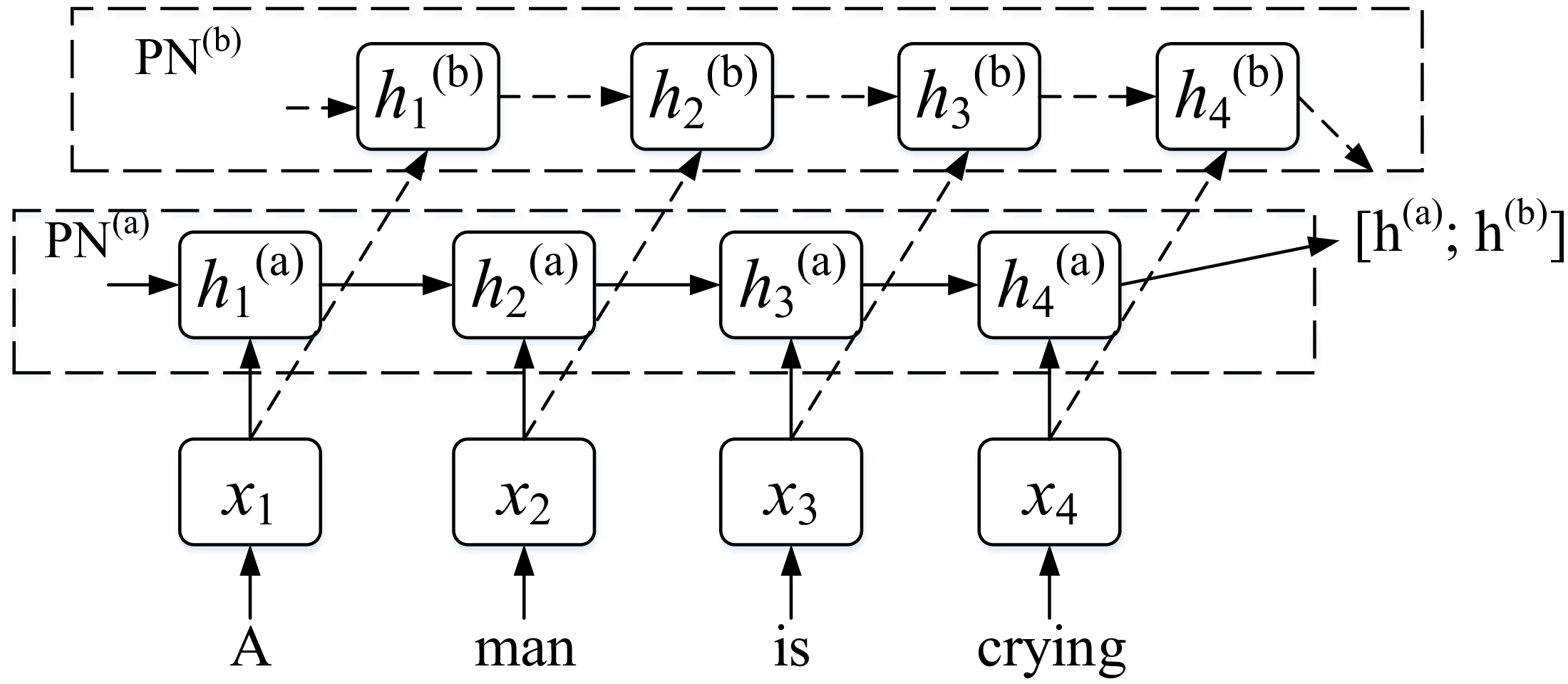
In the SRM, our proposed parallel networks model is outlined in Figure 3. There are two networks, $PN^{(a)}$
and
$PN^{(a)}$
and $PN^{(b)}$
; the hidden layer dimensions of the two networks are different. Based on the parallel networks framework, we design two sentence representation models: context constrained LSTM (CC-LSTM) and Adorned skeleton LSTM (AS-LSTM). Both of these models are based on the BiLSTM and attention mechanisms.
$PN^{(b)}$
; the hidden layer dimensions of the two networks are different. Based on the parallel networks framework, we design two sentence representation models: context constrained LSTM (CC-LSTM) and Adorned skeleton LSTM (AS-LSTM). Both of these models are based on the BiLSTM and attention mechanisms.
BiLSTM model and Attention mechanism.

3.2.1 BiLSTM
LSTM (Hochreiter and Schmidhuber Reference Hochreiter and Schmidhuber1997) is a variant of a RNN. It is mainly used to solve the problem of vanishing gradient. The LSTM model can selectively retain context information through control mechanisms such as input gates, forget gates, and output gates, and it can capture long-distance dependencies in the text. Many variations of LSTM have been applied to natural language processing tasks, such as MT, question-answering systems, and sentence classification. Bidirectional LSTM is one variant, which can effectively obtain the features before and after the current word. BiLSTM mainly consists of three representation layers: an embedding layer, a BiLSTM layer, and an output layer. Figure 2 shows the basic structure of BiLSTM.
3.2.2 Attention mechanism
Transformers and BERT have contributed new state-of-the-art results to various NLP tasks. The attention layer is depicted in Figure 2. Let O be a matrix consisting of the hidden layer vectors $[O_1O_2\ldots O_n]$
in the hidden layer, and O is the input of the attention layer. The attention-based method represents the sentence, including sentence skeleton information, as a weighted sum of these hidden layer vectors.
$[O_1O_2\ldots O_n]$
in the hidden layer, and O is the input of the attention layer. The attention-based method represents the sentence, including sentence skeleton information, as a weighted sum of these hidden layer vectors.
 \begin{equation} A = \tan h(O) \end{equation}
 \begin{equation} \alpha = softmax(\omega _T * A) \end{equation}
 \begin{equation} S_1 = \tan h(O * \alpha ^T) \end{equation}
Here, $\alpha$
is the normalised weight vector, and
$\alpha$
is the normalised weight vector, and $\omega$
is a parameter vector.
$\omega$
is a parameter vector. $S_1$
is the initial state,
$S_1$
is the initial state, $S_1 = Att(X;\; \theta _1)$
, and
$S_1 = Att(X;\; \theta _1)$
, and $\theta _1$
represents all the parameters in this method.
$\theta _1$
represents all the parameters in this method.
The overall process of parallel networks, $PN^{(a)}$
and
$PN^{(a)}$
and $PN^{(b)}$
, have the same input, but the hidden layer dimensions are different: sentence representation from an output concatenation of
$PN^{(b)}$
, have the same input, but the hidden layer dimensions are different: sentence representation from an output concatenation of $PN^{(a)}$
and
$PN^{(a)}$
and $PN^{(b)}$
.
$PN^{(b)}$
.

3.2.3 Parallel networks
The proposed parallel networks model is outlined in Figure 3. There are two networks, $PN^{(a)}$
and
$PN^{(a)}$
and $PN^{(b)}$
, which process the same sentence but have different hidden layer dimensions for obtaining features from multiple levels. Comparing the two networks, the input word embedding for
$PN^{(b)}$
, which process the same sentence but have different hidden layer dimensions for obtaining features from multiple levels. Comparing the two networks, the input word embedding for $PN^{(a)}$
and
$PN^{(a)}$
and $PN^{(b)}$
are the same at each step. When generating hidden layers,
$PN^{(b)}$
are the same at each step. When generating hidden layers, $PN^{(a)}$
uses high-dimensional weight vectors, with hidden layers having higher dimensions. On the contrary,
$PN^{(a)}$
uses high-dimensional weight vectors, with hidden layers having higher dimensions. On the contrary, $PN^{(b)}$
uses low latitude weight vectors, and the hidden layer dimensions are relatively low.
$PN^{(b)}$
uses low latitude weight vectors, and the hidden layer dimensions are relatively low.
The final sentence representation is obtained by concatenating the output results of $PN^{(a)}$
and
$PN^{(a)}$
and $PN^{(b)}$
. In the experiment, the parallel networks model used two dimensions of hidden layers, 900 and 300, respectively. The experiment proved that the 300-dimension hidden layer performed better on short sentences, while the 900-dimension hidden layer had better results on long sentences.
$PN^{(b)}$
. In the experiment, the parallel networks model used two dimensions of hidden layers, 900 and 300, respectively. The experiment proved that the 300-dimension hidden layer performed better on short sentences, while the 900-dimension hidden layer had better results on long sentences.
3.2.4 Context constrained LSTM (CC-LSTM)
The main idea of context constrained LSTM (CC-LSTM) is to build a sentence representation by constrained word context. In this way, it is expected to get more relevant context for the current word. In CC-LSTM, there is a two-level structure:
-
1. Contextual representation layer which builds contextual representation using skeleton words as the boundary.
-
2. Sentence representation layer which gets sentence representation with contextual representation as input.
-
• Contextual representation layer: The skeleton word has a closer relationship with the modifier phrase in the context and the nearby skeleton word. As a qualifier word, its main function is to modify the skeleton word of the context, so its context mainly includes the words between the two skeleton words before and after. Take the sentence in Figure 4 as an example: “
$dog$
” is the skeleton word, which is more closely related to “
$a$
,” “
$brown$
,” and “
$is$
.” “
$In$
” is a qualifier word; “
$is$
” and “
$grass$
” are the same distance from it, but “
$in$
” and “
$grass$
” are more closely related because they are in the same constrained space.


CC-LSTM translates the actions obtained from PNet to a SRM. Formally, given a sentence $W = w_1w_2{\cdots }w_n$
, there is a corresponding action sequence
$W = w_1w_2{\cdots }w_n$
, there is a corresponding action sequence $A = a_1a_2{\cdots }a_n$
obtained from PNet. In this setting, each action
$A = a_1a_2{\cdots }a_n$
obtained from PNet. In this setting, each action $a_i$
at word position
$a_i$
at word position $x_i$
is chosen from {
$x_i$
is chosen from { $qualifier$
,
$qualifier$
, $skeleton$
}, where
$skeleton$
}, where $qualifier$
indicates that the word has a modification function in a sentence, and a
$qualifier$
indicates that the word has a modification function in a sentence, and a $skeleton$
means that the word is skeleton word and acts as a boundary of context.
$skeleton$
means that the word is skeleton word and acts as a boundary of context.
Examples for context constrained LSTM (CC-LSTM).

To limit the word context through the skeleton words, each word will get a variable-length context window. In order for context representation to work in the BiLSTM model, we need to map variable-length contexts to fixed-length spaces. We use the LSTM to map the variable-length context. Taking $w_6$
in Figure 4 as an example, the upper boundary of
$w_6$
in Figure 4 as an example, the upper boundary of $w_6$
is
$w_6$
is $w_5$
, and the lower boundary is
$w_5$
, and the lower boundary is $w_9$
. The context representation is as follows Eq. 8–10:
$w_9$
. The context representation is as follows Eq. 8–10:
 \begin{equation} c_6^1 = LSTM(w_5, w_6) \end{equation}
 \begin{equation} c_6^2 = LSTM(w_6, w_7, w_8, w_9) \end{equation}
 \begin{equation} c_6 = c_6^1 \oplus c_6^2 \end{equation}
where LSTM denotes the LSTM model, $w_6$
is the embedding of “
$w_6$
is the embedding of “ $in$
,”
$in$
,” $c_6$
is the context representation of “
$c_6$
is the context representation of “ $in$
,” and
$in$
,” and $\oplus$
indicates vector concatenation. The contextual representation of other words is similar to
$\oplus$
indicates vector concatenation. The contextual representation of other words is similar to $w_6$
. We need to generate a contextual representation of each word one by one.
$w_6$
. We need to generate a contextual representation of each word one by one.
-
• The sentence representation layer. The sentence representation layer contains two parts: BiLSTM and an attention mechanism. The input of BiLSTM is the context representation, and its hidden layers are used as the input of the attention mechanism.
(11)
\begin{equation} o = BiLSTM(c_1, c_2,\ldots , c_n) \end{equation}
(12)where
\begin{equation} S = att(o) \end{equation}
$o$
denotes hidden layers of BiLSTM, it contains multiple outputs;
$S$
is sentence representation.


3.2.5 Adorned skeleton LSTM (AS-LSTM)
Adorned skeleton LSTM (AS-LSTM) first identifies the skeleton word of the sentence and then constructs the skeleton representation of the current skeleton word through the qualifiers of the skeleton word. We define the qualifiers for the current skeleton word to be the word between the two skeletons before and after it. This process is implemented by sampling an action in $\{qualifier, skeleton\}$
at each word position, where
$\{qualifier, skeleton\}$
at each word position, where $skeleton$
indicates that a word is the skeleton of a sentence and
$skeleton$
indicates that a word is the skeleton of a sentence and $qualifier$
means the word has a modification function.
$qualifier$
means the word has a modification function.
Examples for Adorned skeleton LSTM (AS-LSTM).

As shown in Figure 5, the AS-LSTM adopts a two-level structure: a skeleton representation layer and a sentence representation layer.
-
• Skeleton representation layer: In the skeleton representation layer, the skeleton words divide the sentence into several independent fragments; each fragment includes a skeleton word and several qualifier words of the skeleton word. The skeleton word needs to be combined with qualifier words to reflect its true meaning. Therefore, we need to construct the skeleton representation based on the qualifier. The qualifiers of a skeleton are divided into pre-modifiers and post-modifiers according to their positions. A pre-modifier and a post-modifier are allowed to be null. The pre-modifier and skeleton word generate the top skeleton representation. The post-modifier and skeleton word generate the tail skeleton representation. Take the skeleton word “
$dog$
” as an example. “
$dog$
” is a skeleton word; its pre-modifier is “
$A$
” and “
$brown$
,” and its post-modifier is none.(13)
\begin{equation} f_1 = BiLSTM(w_1, w_2, w_3) \end{equation}
(14)
\begin{equation} b_1 = BiLSTM(w_3) \end{equation}
(15)where
\begin{equation} sk_1 = att(f_1, b_1) \end{equation}
$BiLSTM$
denotes the BiLSTM model,
$f_1$
is the skeleton representation of the pre-modifier,
$b_1$
is the skeleton representation of the post-modifier, and
$sk_1$
is the skeleton representation of “
$dog$
.” The attention mechanism is applied to give different weights to
$f_1$
and
$b_1$
that have different effects on the skeleton words.


-
• Sentence Representation Layer: The sentence representation layer contains two parts: a BiLSTM and an attention mechanism. The input of BiLSTM is the skeleton representation, and its hidden layers are used as the input of the attention mechanism.
(16)
\begin{equation} o = BiLSTM(sk_1, sk_2, sk_3) \end{equation}
(17)where
\begin{equation} S = att(o) \end{equation}
$o$
denotes hidden layers of BiLSTM, it contains multiple outputs;
$S$
is sentence representation.


3.3 Similarity calculation model
Given a sentence pair, we predict a real-valued similarity score in some range $[1, K]$
, where
$[1, K]$
, where $K$
$K$ $\gt$
1 and is an integer. The sequence
$\gt$
1 and is an integer. The sequence $\{1, 2, {\cdots }, K\}$
is some ordinal scale of similarity, where higher scores indicate greater degrees of similarity, and we allow real-valued scores to account for ground-truth ratings that are the average over the evaluations of several human annotators.
$\{1, 2, {\cdots }, K\}$
is some ordinal scale of similarity, where higher scores indicate greater degrees of similarity, and we allow real-valued scores to account for ground-truth ratings that are the average over the evaluations of several human annotators.
Firstly, SRM generates a representation of sentence pairs. Given these sentence representations, we predict the similarity score $\hat {y}$
using a neural network that considers both the distance and angle between the pair (
$\hat {y}$
using a neural network that considers both the distance and angle between the pair ( $h_L$
,
$h_L$
, $h_R$
):
$h_R$
):
 \begin{equation} h_{\times } = h_L * h_R \end{equation}
 \begin{equation} h\_ = |h_L - h_R| \end{equation}
 \begin{equation} h_s = \sigma \big(W^{(\times )}h_{\times } + W^{(+)h\_ + b^{(h)}}\big) \end{equation}
 \begin{equation} \hat {p}\theta = softmax\big(W^{(p)}h_s + b^{(p)}\big) \end{equation}
 \begin{equation} \hat {y} = r^T\hat {p}\theta \end{equation}
where $r^T$
=
$r^T$
= $[1 2 . . . K]$
and the absolute value function is applied elementwise. The use of both distance measures
$[1 2 . . . K]$
and the absolute value function is applied elementwise. The use of both distance measures $h_{\times }$
and
$h_{\times }$
and $h\_$
is empirically motivated: it is found that the combination outperforms the use of either measure alone. The multiplicative measure
$h\_$
is empirically motivated: it is found that the combination outperforms the use of either measure alone. The multiplicative measure $h_{\times }$
can be interpreted as an elementwise comparison of the signs of the input representation. The subtractive measure
$h_{\times }$
can be interpreted as an elementwise comparison of the signs of the input representation. The subtractive measure $h\_$
can measure the difference between the input representation
$h\_$
can measure the difference between the input representation $\hat {p}\theta$
and the vector representation of our predicted outcome.
$\hat {p}\theta$
and the vector representation of our predicted outcome. $\hat {y}$
is predicted outcome.
$\hat {y}$
is predicted outcome.
The cost function is the regularised KL-divergence (Solomon and Leibler Reference Solomon and Leibler1951) between p and $\hat {p}\theta$
:
$\hat {p}\theta$
:
 \begin{equation} J(\theta ) = \dfrac {1}{m}\sum ^{m}_{k=1}KL(p^k||\hat {p}\theta ^k) + \dfrac {\lambda }{2}||\theta ||^2_2 \end{equation}
where m is the number of training pairs and the superscript k indicates the kth sentence pair. Note that we use the same KL-loss function and sparse target distribution technique as (Tai et al. Reference Tai, Socher and Manning2015).
4. Experiments
4.1 Tasks and datasets
The datasets SICK and SemEval are used in the experiment.
4.1.1 Sentences involving compositional knowledge (SICK) dataset
The dataset is from the 2014 SemEval competition (Marelli et al. Reference Marelli, Bentivogli, Baroni, Bernardi, Menini and Zamparelli2014) and consists of 9927 sentence pairs, 4500 pairs of training set, 500 pairs of validation set, and 4927 pairs of test set. Each sentence pair is scored manually, and the relatedness score range is [1, 5]. With higher scores indicating the two sentences are more closely related.
4.1.2 STS benchmark dataset
The dataset comprises 8628 sentence pairs. The STS Benchmark dataset was used in the STS tasks and organised in the context of SemEval between 2012 and 2016. The selection of datasets includes text from image captions, news headlines, and user forums. 8,628 different sentence pairs of varying
The Microsoft Video Paraphrase Dataset (MSRVID) (Agirre et al. Reference Agirre, Diab, Cer and Gonzalez-Agirre2012) was collected for the 2012 SemEval competition and consists of 1,500 pairs of short video descriptions which were then annotated. Among them, 1000 sentence pairs are used as a training corpus, 250 sentence pairs as a test corpus, and 250 sentence pairs as a validation corpus.
4.1.3 Hyperparameters and training detail
Hyperparameters. Dropout (Srivastava, Salakhutdinov, and Hinton Reference Srivastava, Salakhutdinov and Hinton2013) is applied to embedding hidden states with a rate of 0.5. All models are optimised using the Adam optimiser (Kingma and Jimmy Reference Kingma and Jimmy2015), with an initial learning rate of 0.0014 and a decay rate of 0.95. A batch size of 32 is adopted. Sentences with similar lengths are batched together. The L2 regularisation parameter is set to 0.00001.
Training detail. The initialisation of word vectors consists of three types of vectors. The three types of vectors mainly include GloVe (Pennington, Socher, and Manning Reference Pennington, Socher and Manning2014) embeddings, trained word vector from the word2vec (Mikolov et al. Reference Mikolov, Chen, Corrado and Dean2013) model, and trained POS vector from the word2vec model. In the experiment, these three vectors are spliced. Among them, the word vector training corpus based on word2vec is the SICK dataset and STS benchmark dataset. Similarly, the POS tagging sequence required by the POS vector also comes from the POS of the SICK dataset and STS benchmark dataset. The POS tagging tool we use is NLTK. The initial hidden layer required for training is randomly generated. In order to ensure the stability of the initial hidden layer during testing, we uniformly use the mean of the hidden layer vectors generated during the training process.
-
• Rpos setting: The Rpos function is set based on the weight of the corresponding POS for each word in the sentence. In the corpus, the POS of each word corresponds to a weight, which is calculated based on the corpus annotated in the SICK corpus validation set. That is, the proportion of each POS as the backbone in the corpus is the weight of each POS. Due to the Rpos function assisting reinforcement learning to learn the optimal solution faster, the value of Rpos being too high can interfere with the reward of the result and affect the PNet. To prevent the reward values calculated based on POS weights from being too large, multiply them by a balance parameter. The parameter is the average value of loss during pre-training.
-
• Reward_L: The reward_L function is summarised based on the corpus annotated in the validation set. In statistics, the sentence length in the corpus is used as the horizontal axis, and the number of skeletons in the sentence is used as the vertical axis. The points formed are denoted as
$(x, y)$
. When labelling points in coordinates, there is a high coincidence rate because the number of skeleton
$y$
and sentence length
$x$
are both integers. In order to highlight the density of the points, a number between [–0.5, 0.5] is randomly added to the number of skeleton
$y$
and sentence length
$x$
, which is equivalent to randomly marking points in a circle with
$(x, y)$
as the centre and 0.5 as the radius.


The points composed of the length of each sentence and the number of skeletons in the sentence are marked in Figure 6. And three lines were set, $y_1$
,
$y_1$
, $y_2$
, and
$y_2$
, and $y_3$
. Among them,
$y_3$
. Among them, $y_1$
and
$y_1$
and $y_2$
are boundary functions, and
$y_2$
are boundary functions, and $y_3$
is the objective function. The points in the figure are almost all concentrated between the lines
$y_3$
is the objective function. The points in the figure are almost all concentrated between the lines $y_1$
and
$y_1$
and $y_2$
; therefore, we choose a piecewise function for Reward_L. At the coordinate points between lines
$y_2$
; therefore, we choose a piecewise function for Reward_L. At the coordinate points between lines $y_1$
and
$y_1$
and $y_2$
, we believe that the number of skeletons corresponding to the sentence length is relatively reasonable. Therefore, when calculating the error with the objective function in this area, we multiply it by a coefficient; the coefficient was 0.3 in the experiment. At points outside of lines
$y_2$
, we believe that the number of skeletons corresponding to the sentence length is relatively reasonable. Therefore, when calculating the error with the objective function in this area, we multiply it by a coefficient; the coefficient was 0.3 in the experiment. At points outside of lines $y_1$
and
$y_1$
and $y_2$
, we consider them unreasonable and use the original values when calculating the error with the objective function.
$y_2$
, we consider them unreasonable and use the original values when calculating the error with the objective function.
The relationship between the number of skeletons and sentence length in the annotated corpus.

4.2 Results on SICK dataset
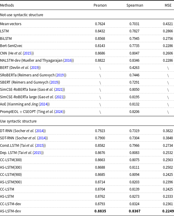
The results are summarised in Table 1. The model uses Pearson’s, Spearman’s, and MSE as evaluation metrics. In the experiment, we did not choose to expand the external training corpus, so we chose the experimental results under the same training corpus for comparison. In addition, due to some researchers choosing to incorporate validation set data into the training set to train the training model during experiments, we also trained and compared the results under the same training data. We used the suffix ‘dev’ as a marker for these results. In each column, the best result is shown in bold.
Test set results on the SICK, MALSTM-dev model, CC-LSTM-dev model, and AS-LSTM-dev model use 5000 sentence pairs as a training corpus, including the SICK training set and SICK validation set. Others only use the training set as the training corpus. (300) and (900) represent that the models select 300-dimensional and 900-dimensional hidden layers in the process of training the corpus, respectively.

The experiment involves two setups: not using syntactic structure vs using syntactic structure in the process of constructing the sentence representation. In the model of not-using syntactic structure, it is observed that the MALSTM leads to a huge improvement. SimCSE and BERT also used a large amount of corpus for pre-training, but Bert’s results on the SICK dataset were not satisfactory. SimCSE added a comparative model on top of Bert’s pre-training model, significantly improving the test results. In models that use syntactic information, the best results are not achieved for Tree-LSTM, but the Tree-LSTM improves 1 point compared with the LSTM baseline model.
Skeleton-based approaches do not rely on parse trees but POS to assist skeleton word identification. From the experimental result, AS-LSTM exceeds all the above models under the same training corpus. Even with a single hidden layer, AS-LSTM (900) achieves excellent results. In addition, compared with models using only a single hidden layer, the results are significantly improved in the parallel networks.
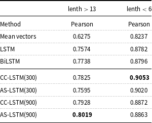
In order to find out the reason why the PN can improve the calculation results of sentence similarity, they designed experiments to select a 300-dimensional hidden layer and a 900-dimensional hidden layer for the LSTM model. In the experiment, choose two different sets of data, including length of sentence pairs greater than 13 (393 pairs) and less than 6 (195 pairs). Experimental results in Table 2 show that the 300-dimensional hidden layer has better results in short sentences under the same model. To the contrary, higher dimensions have excellent performance on long sentence pairs.
Compare the results of sentences of different lengths, (300) and (900), representative models. Select 300-dimensional and 900-dimensional hidden layers in the process of training the corpus, respectively

In the CC-LSTM and AS-LSTM models, the skeleton word decomposes the sentence into multiple parts, reducing the connection of words between different parts. Both of these models perform relatively well in longer sentence pairs.
4.3 Results on STS benchmark dataset
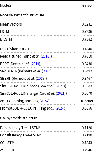
Our results on the STS benchmark dataset are summarised in Table 3. Compared with the results obtained by SimCSE-RoBERTa in large-scale corpus training, the results obtained only in the training set are relatively poor. After analysis, the main reasons are twofold. Firstly, the STS corpus contains too many types of sentences, and there are significant differences between different types of sentences. Secondly, the number of sentences in each type is too small, and SimCSE-RoBERTa is trained on a large-scale corpus to obtain more information. Although our results are worse than SimCSE-RoBERTa, SBERT and SRoBERTa, they are much better than other models trained only in the training corpus. In each column, the best result is shown in bold.
Results on the STS benchmark dataset: “*” indicates that the result comes from the internet page

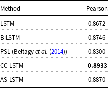
Our results on the MSRVID data are presented in Table 4. The results show the CC-LSTM model has a better performance in short sentence pairs.
Results on MSRVID dataset

4.4 Result analysis
To investigate how the discovered skeleton sentence influences sentence similarity calculation performance, we present result analysis from quantitative perspectives. Statistics show that there is a certain difference between the skeleton information obtained through reinforcement learning and the manually annotated skeleton information. However, from the experimental results, skeleton-based approaches are higher than other models that use syntactic information, so we believe that the skeleton information obtained through reinforcement learning is more suitable for the STS task.
We present further analysis on what POS is identified as the skeleton word. We investigate the impact of part-of-speech tagging on skeleton recognition.
Next, further analyse which POS is easily identified as a skeleton word. And the impact of part of speech tagging on skeleton recognition was studied.
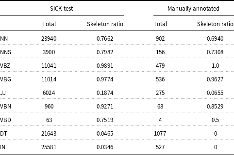
For words of different POS, the probability of being identified as the skeleton of the sentence is also different. We separately count the SICK dataset test results and the sentences marked with the skeleton information in the SICK dataset. Among them, the sentences marked with the skeleton information in the SICK dataset are 495 sentences, and skeleton information is manually labelled. Table 5 shows the total number of important POS in the dataset and the proportion of skeletons. We find the following POS are more likely to be identified as the skeleton word: NN (Noun, singular), NNS (Noun, plural), VBG (Verb, gerund or present participle), VBZ (Verb, 3rd person singular present), VBD (Verb, past tense), and VBN (Verb, participle). In addition, some POS with a low probability of being identified as the skeleton include CD (Cardinal number), DT (Determiner), IN (Preposition or subordinating conjunction), JJ (Adjective), and RB (Adverb).
The frequency of various POS in the dataset and the ratio of the skeleton

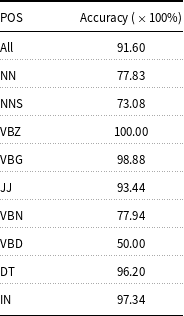
In this skeleton-based approach, the reinforcement learning can obtain the skeleton of the sentence in the model training and then use the skeleton information to construct the sentence representation. In order to verify the quality of the sentence skeleton recognition results, we use sentences annotated with skeleton information as the standard skeleton tagging dataset for experiments. Table 6 shows the accuracy of the skeleton annotation.
The accuracy of skeleton recognition and the accuracy of each POS skeleton recognition

According to the specific analysis of the results based on the annotated corpus, the accuracy of JJ, VBG, VBD, CD, IN, and other parts of speech recognition achieves a satisfactory high level, but the accuracy of noun and NNS recognition is comparatively low.
AS-LSTM_N only uses the loss function as the reward function. AS-LSTM_L represents the addition of Reward_L to the reward function in AS-LSTM_N. AS-LSTM_P represents the addition of Rpos to the reward function in AS-LSTM_N. AS-LSTM_A indicates that all rewards have been added. BiLSTM represents using only the BiLSTM model to obtain results. The horizontal axis represents the epoch, and the vertical axis represents the corresponding result of the epoch.

4.5 Ablation studies
Figure 7 presents ablation studies for the reward function. The reward function is divided into three parts: the loss function, Reward_L, and Rpos. The loss function is the foundation of the reward function, Reward_L, and Rpos plays a certain auxiliary role. We conduct ablation studies on the AS-LSTM to further analyse the effectiveness of each reward. Compared to using only the loss function as a reward, AS-LSTM_L and AS-LSTM_P have improved the results by 0.06 and 0.22, respectively. They not only have some improvement in results but also greatly reduce the epoch when achieving the best results. Compared to AS-LSTM_L, AS-LSTM_P not only achieves higher and more robust results but also has a lower epoch when obtaining the best results. Adding Reward_L to AS-LSTM_P resulted in an increase of 0.11 in AS-LSTM_A results and a decrease of 3 epochs for optimal results. In addition, in Figure 6, we can also observe that although the BiLSTM model achieves relatively high results quickly, it is particularly prone to overfitting. The AS-LSTM model does not exhibit this performance and exhibits more robust results.
5. Conclusion
This paper presents a skeleton-based reinforcement learning method which learns sentence representation by discovering sentence skeletons. In the framework of the parallel networks, there are two representation models: CC-LSTM and AS-LSTM. CC-LSTM builds the sentence representation by constraining word context and uses the skeleton as the boundary of the word context, restricting the acquisition of the word context. In the AS-LSTM model, words in the sentence are first classified into skeleton words or modifiers, and then the skeleton representation is constructed. AS-LSTM constructs a sentence vector through skeleton representation. Extensive experiments show that our method has outstanding performance, which not only finds the skeleton information of the sentence but also exploits the skeleton information to improve the accuracy of similarity calculation.
6. Limitations
The limitations of our work can be stated from three perspectives. First, the current generated sentence skeleton contains relatively little structural information. It can be future work to explore how to automatically generate the more complex grammar. Secondly, the current model only has two action spaces. In future work, we will try to design multiple action spaces to complete the experiment. Thirdly, the AS-LSTM model is not very friendly to sentences containing negative words. In future work, we will attempt to identify negative words as the skeleton as much as possible for experimentation.
Acknowledgements
This work was supported by the National Natural Science Foundation of China (No.U1936109).






 Open access

