


1. Introduction
In practice, turbulent boundary layers (TBLs) are typically subjected to incoming turbulence. In the case of an external TBL, both freestream turbulence (FST) and the TBL develop downstream while interacting with each other. This occurs both in nature and in industrial applications, for example an open channel downstream of a water reservoir such as a hydropower dam, in which the TBL is affected by upstream disturbances in the flow.
A wealth of experimental studies, and more recently, several direct numerical simulations (DNS) have been dedicated to gaining insights into the effects of FST on the statistics of TBLs. In general, FST is known to increase the friction velocity ( $U_\tau$) of zero-pressure-gradient (ZPG) TBLs and suppress the wake region of the mean velocity profile, while having minimal effect on the log region (e.g. Blair Reference Blair1983; Hancock & Bradshaw Reference Hancock and Bradshaw1983; Castro Reference Castro1984; Thole & Bogard Reference Thole and Bogard1996; Dogan, Hanson & Ganapathisubramani Reference Dogan, Hanson and Ganapathisubramani2016; Dogan, Hearst & Ganapathisubramani Reference Dogan, Hearst and Ganapathisubramani2017; Esteban et al. Reference Esteban, Dogan, Rodríguez-López and Ganapathisubramani2017; Hearst, Dogan & Ganapathisubramani Reference Hearst, Dogan and Ganapathisubramani2018; Dogan et al. Reference Dogan, Hearst, Hanson and Ganapathisubramani2019). Recently, using laser Doppler velocimetry at several streamwise locations, Jooss et al. (Reference Jooss, Li, Bracchi and Hearst2021) investigated the coevolution of a ZPG-TBL and FST. They showed that by moving downstream, some of the FST effects, e.g. the wake suppression, weakened due to the decay of the FST intensity ( $u'_\infty /U_\infty$, where $u'_\infty$ denotes the standard deviation of the streamwise velocity fluctuations and $U_\infty$ indicates the mean streamwise velocity, both in the freestream). They stated that, in addition to friction Reynolds number ( $Re_\tau = U_\tau \delta /\nu$, where $\delta$ is the boundary layer thickness and $\nu$ denotes the kinematic viscosity of the fluid) and $u'_\infty /U_\infty$, the coevolution of the TBL and FST is another decisive parameter that should be remarked on for characterising a TBL subjected to FST.
The instantaneous structure of TBLs is nowadays known to be populated by regions with uniform streamwise momentum, known as uniform momentum zones (UMZs). The presence of UMZs in a ZPG-TBL was originally reported by Meinhart & Adrian (Reference Meinhart and Adrian1995) using particle image velocimetry (PIV) measurements, where they argued that UMZ edges coincide with high negative vorticity streaks. This was confirmed by later studies of Eisma et al. (Reference Eisma, Westerweel, Ooms and Elsinga2015), de Silva, Hutchins & Marusic (Reference de Silva, Hutchins and Marusic2016) and de Silva et al. (Reference de Silva, Philip, Hutchins and Marusic2017). Adrian, Meinhart & Tomkins (Reference Adrian, Meinhart and Tomkins2000) studied the characteristics of UMZs extensively, referring to them as signatures of hairpin vortices. They identified the UMZs using the histogram of the instantaneous streamwise velocity, where each UMZ was represented as a peak in the histogram, referred to as the ‘modal velocity’. The same approach was utilised later by de Silva et al. (Reference de Silva, Hutchins and Marusic2016) to study the structural properties of these zones over a wide range of  $Re_\tau \approx 10^3$– $10^4$ using several PIV databases. The authors argued that the number of the UMZs present in a ZPG-TBL increases logarithmically with $Re_\tau$. In addition, the authors found no discernible correlation between the instantaneous location of the TBL edge, which they referred to as the instantaneous boundary layer height, and the number of UMZs. Instead, they observed that variations in the instantaneous boundary layer height influenced the thickness of outer UMZs located farther from the wall. Given the importance of UMZs in the structural organisation of a boundary layer on the one hand, and the prevalence of PIV and advancements in DNS on the other, it is of no surprise that the study of UMZs has been a hot topic recently. This is reflected by multiple studies investigating the UMZs in turbulent channel (Kwon et al. Reference Kwon, Philip, de Silva, Hutchins and Monty2014; Anderson & Salesky Reference Anderson and Salesky2021; Zheng & Anderson Reference Zheng and Anderson2022; Huang et al. Reference Huang, Jie, Xu and Zhao2024) and pipe flows (Chen, Chung & Wan Reference Chen, Chung and Wan2020; Gul, Elsinga & Westerweel Reference Gul, Elsinga and Westerweel2020), and their temporal evolution in TBLs (Laskari et al. Reference Laskari, de Kat, Hearst and Ganapathisubramani2018; Laskari & McKeon Reference Laskari and McKeon2021). In a recent study, using PIV measurements of a ZPG-TBL subjected to two different FST intensities, Hearst et al. (Reference Hearst, de Silva, Dogan and Ganapathisubramani2021) reported the presence of UMZs. They argued that the number of UMZs decreases with increasing $u'_\infty /U_\infty$ and that the distribution of the modal velocities for the inner UMZs, i.e. closer to the wall, remains intact when FST is present, suggesting the near-wall structures are robust to FST. Asadi, Kamruzzaman & Hearst (Reference Asadi, Kamruzzaman and Hearst2022a) investigated the effects of incoming turbulence on the central UMZ, i.e. the quiescent core, of turbulent channel flow, stating that the incoming turbulence manipulates the momentum content of the core, which in turn gives rise to low-momentum and high-momentum core states.
A prerequisite for correctly identifying UMZs using the histogram method is to discard the instantaneous freestream (de Silva et al. Reference de Silva, Hutchins and Marusic2016). This in itself requires the boundary between the instantaneous TBL and freestream flow to be identified. A TBL and an irrotational freestream flow are in contact through the so-called turbulent/non-turbulent interface (TNTI). The characteristics of the TNTI were first described in the seminal work of Corrsin & Kistler (Reference Corrsin and Kistler1955), pivoting around the essential fact that the vorticity is absent in the irrotational non-turbulent freestream. Even though the task of identifying the instantaneous TNTI, i.e. separating the instantaneous TBL from the irrotational freestream, would sound straightforward, it is usually challenging due to the presence of noise obscuring the exact location of this fine interface, especially in experimental measurements. Some of the previous studies that have identified an interface between a turbulent flow and a non-turbulent freestream are listed in table 1. DNS benefits from high spatial resolution, and well-defined boundary and initial conditions, which facilitate the use of a threshold to identify the TNTI layer as an iso-surface with a low vorticity magnitude. In DNS of ZPG-TBLs, the vorticity threshold value is usually chosen using the joint probability density function (j.p.d.f.) of the wall-normal location ( $\kern0.7pt y$) and the logarithm of the normalised vorticity magnitude $|\omega |^* = |\omega | (\nu /U_\tau ^2) \sqrt {\delta _{99}^+}$, where $\delta _{99}$ indicates the boundary layer thickness based on the height at which the mean velocity reaches within 99 % of $U_\infty$ (Jiménez et al. Reference Jiménez, Hoyas, Simens and Mizuno2010; Borrell & Jiménez Reference Borrell and Jiménez2016; Lee, Sung & Zaki Reference Lee, Sung and Zaki2017). An alternative approach would be to plot the volume of turbulent region as a function of the vorticity threshold (e.g. da Silva et al. Reference da Silva, Hunt, Eames and Westerweel2014; Krug et al. Reference Krug, Holzner, Marusic and van Reeuwijk2017; Watanabe, Zhang & Nagata Reference Watanabe, Zhang and Nagata2018; Zhang, Watanabe & Nagata Reference Zhang, Watanabe and Nagata2023). Nevertheless, DNS is often limited to relatively low Reynolds numbers, small computational volumes and simple geometries. With recent advances in digital cameras and computer power, experimental measurements have been performed to investigate the TNTI at higher Reynolds numbers. Planar PIV measurements have been the most common experimental method to study the spatial characteristics of boundary layers, e.g. UMZs and TNTIs. The TNTI surface is manifested as a contorted line in two-dimensional (2-D) PIV measurements. Although some experimental studies opted for the spanwise vorticity threshold to identify the TNTI (e.g. Eisma et al. Reference Eisma, Westerweel, Ooms and Elsinga2015), it is quite difficult to identify instantaneous TNTIs in PIV fields using a vorticity threshold, as the accuracy of vorticity estimations is typically limited by low spatial resolution and PIV noise (Reuther & Kähler Reference Reuther and Kähler2018). Thus, surrogate methods were developed to mark the TNTI based on different flow characteristics, e.g. employing the local turbulent kinetic energy deficit (KED) criterion (Chauhan et al. Reference Chauhan, Philip, de Silva, Hutchins and Marusic2014; Philip et al. Reference Philip, Meneveau, de Silva and Marusic2014), using a passive scalar (Prasad & Sreenivasan Reference Prasad and Sreenivasan1989; Westerweel et al. Reference Westerweel, Fukushima, Pedersen and Hunt2009) and utilising local seeding to mark the turbulent fluid (Reuther & Kähler Reference Reuther and Kähler2018). Moreover, several artificial intelligence methods have been developed recently to separate the turbulent regions from non-turbulent regions of the flow based on machine learning algorithms (Wu et al. Reference Wu, Lee, Meneveau and Zaki2019b; Li et al. Reference Li, Yang, Zhang, He, Deng and Shen2020; Younes et al. Reference Younes, Gibeau, Ghaemi and Hickey2021; Khojasteh, van de Water & Westerweel Reference Khojasteh, van de Water and Westerweel2024).
Some prior studies that identified an interface to distinguish between a turbulent flow and non-turbulent freestream.

The presence of vortical structures in FST raises significant questions regarding the very nature of a TBL/FST interface. First and foremost, does such an interface exist? The concept of an interface separating a TBL from FST was briefly mentioned by Wu et al. (Reference Wu, Moin, Wallace, Skarda, Lozano-Durán and Hickey2017) and investigated in their later work (Wu, Wallace & Hickey Reference Wu, Wallace and Hickey2019a) using DNS of a spatially developing TBL subjected to homogeneous isotropic FST with a maximum  $u'_\infty /U_\infty$ of 3 %. Given that a TBL and decaying FST exhibit distinct vortical organisations, Wu et al. (Reference Wu, Wallace and Hickey2019a) speculated that an interface exists between them. Scholars have been unable to mark the interface using a constant vorticity threshold due to the presence of instantaneous vorticity in FST. Table 2 presents some prior studies that used surrogate methods to identify an interface between two turbulent flows. Wu et al. (Reference Wu, Wallace and Hickey2019a) considered heating the wall in their simulations and using a scalar (normalised temperature values) threshold to identify a surrogate interface. As a means of validating their methodology, they used qualitative comparisons of scalar interfaces with associated vorticity fields as well as the observation of quasi-step jumps across the interface in conditionally averaged profiles of swirling strength and normalised temperature. In a concurrent study, You & Zaki (Reference You and Zaki2019) stated that due to the presence of diffusion on both sides of the interface, the scalar is not a reliable marker to distinguish between the freestream and boundary layer flow. Instead, using a level-set numerical approach, they removed the diffusion effects altogether to identify a sharp virtual interface between FST and the TBL. Although the level-set approach provided a more robust technique to draw instantaneous boundaries between the FST and TBL, it identified a material boundary between the two flows, neglecting the entrainment of the freestream fluid into the boundary layer. Hearst et al. (Reference Hearst, de Silva, Dogan and Ganapathisubramani2021) employed a KED threshold method, similar to the studies of de Silva et al. (Reference de Silva, Hutchins and Marusic2016) and Laskari et al. (Reference Laskari, de Kat, Hearst and Ganapathisubramani2018), to isolate the instantaneous boundary layer flow in their PIV fields. Performing sensitivity analyses, they argued that the trends of their results were insensitive to the threshold choice. In addition, they observed sudden changes in conditionally averaged profiles of velocity and swirling strength across the interface. It is worth mentioning that in turbulent channel flows, the identification of the quiescent core boundary is widely accepted to be momentum-based, indicated by continuous contour lines of constant velocity (Kwon et al. Reference Kwon, Philip, de Silva, Hutchins and Monty2014; Yang, Hwang & Sung Reference Yang, Hwang and Sung2016, Reference Yang, Hwang and Sung2019; Jie et al. Reference Jie, Xu, Dawson, Andersson and Zhao2019; Jie, Andersson & Zhao Reference Jie, Andersson and Zhao2021; Asadi et al. Reference Asadi, Kamruzzaman and Hearst2022a). In addition, Dogan et al. (Reference Dogan, Hearst, Hanson and Ganapathisubramani2019) noted a certain degree of similarity in momentum transport between a TBL subjected to FST and turbulent channel flow. In particular, the wake region of a TBL developing under FST more closely resembles the wake region of a turbulent channel flow than a ZPG-TBL.
Some prior studies that identified an interface to distinguish between two turbulent flows.

Considering the studies mentioned previously, the methodology for correctly identifying an interface separating a TBL from FST is debatable as various scholars have opted for different methods. In addition, the presence of the interface is evaluated less rigorously in experimental measurements, where practical limitations, such as measurement noise and limited spatial resolution, pose formidable obstacles to its identification. To the best of the authors’ knowledge, spatially resolved measurements of a TBL under the influence of FST at multiple streamwise locations do not exist to date. In addition, DNS studies are restricted by computational costs, which in this case limits the Reynolds number (Kozul et al. Reference Kozul, Hearst, Monty, Ganapathisubramani and Chung2020) as well as the number of FST cases (Wu et al. Reference Wu, Wallace and Hickey2019a; You & Zaki Reference You and Zaki2019) tested in the simulations. In this study, three different incoming FST intensities are produced using an active grid, which then are measured with PIV at four different streamwise locations far downstream of the grid, providing new insight into the fluid mechanics of this problem. Solely using PIV measurements, we introduce a new method to identify interfaces that separate structural features of the TBL from FST based on vorticity distributions. The effects of FST on the interface properties and the UMZs within the TBL are highlighted by comparing the active cases with a low-turbulence reference case and, then, the streamwise evolution of the effects is investigated for the cases with FST. The experimental set-up, measurement method and characteristics of the test cases are detailed in § 2. The new interface identification method is introduced and tested in § 3. The effects of FST on the TBL structures as well as the streamwise changes of the effects are discussed in § 4.
2. Experimental procedure
2.1. Experimental set-up
The experiments were carried out in the water channel facility at the Norwegian University of Science and Technology. The details of the facility are described by Jooss et al. (Reference Jooss, Li, Bracchi and Hearst2021) in Appendix A of their article. The test section provides a free-surface open-channel test bed filled to a height of 0.22 m ( $H$) for the present investigation and measures 1.8 m in width and 11 m in length. To trip the boundary layer, a strip of multiscale grip tape with a length of 50 mm in the streamwise direction was placed at the bottom wall immediately downstream of the active grid, spanning the whole width of the test section. To effectively dampen the surface waves created by the motion of the grid bars, two slanted surface plates were installed on both the upstream and downstream sides of the active grid. The plate installed inside the contraction measured 1.5 m in the streamwise direction and was cut to the shape of the contraction out of a 6-mm-thick marine-grade aluminium sheet. The surface plate placed inside the test section was a rectangular 10-mm-thick acrylic plate, measuring 1.8 m in width and extending 3 m downstream (see figure 1 for a schematic).
Schematic of the water channel, active grid, and measurement set-up.

Since the introduction of active grids, pioneered by the seminal work of Makita (Reference Makita1991), they have become powerful tools for researchers to effectively tailor the turbulent characteristics of flows. Applying minor modifications, the same active grid utilised by Jooss et al. (Reference Jooss, Li, Bracchi and Hearst2021) was used to set the incoming flow conditions in the present investigation (see Jooss et al. Reference Jooss, Li, Bracchi and Hearst2021, Appendix B, for detailed information regarding the design and operation of the grid). In short, the grid consists of 18 vertical and 10 horizontal bars each of which was connected to a stepper motor, allowing for the independent control of each bar. The agitator wings were built in a square shape out of 1-mm-thick stainless steel sheets with holes cut out of them to reduce the blockage ratio. In order for the grid to fit the cross-section of the flow, the configuration of the wings was modified compared with that used by Jooss et al. (Reference Jooss, Li, Bracchi and Hearst2021). This included using only two horizontal bars and installing an additional row of half-wings on the vertical bars (figure 1). The grid mesh length ( $M$), i.e. the distance between the grid bars, was 100 mm. Fully random sequences of the rotational period, acceleration and velocity as described by Hearst & Lavoie (Reference Hearst and Lavoie2015) were fed to the motors. The mean rotational velocity was changed between test cases to create different incoming flow conditions as described in § 2.3.
2.2. Experimental measurements
Planar PIV measurements were performed in streamwise–wall-normal planes in the spanwise centre of the channel. To evaluate the streamwise evolution of the flow, four streamwise planes were examined located at  $X = 55M$, $65M$, $72M$ and $85M$, where $X$ represents the streamwise axis of the global coordinate system, whose origin is at the active grid location. Polystyrene particles with a mean diameter of 40 $\mathrm {\mu }$m (Dynoseeds TS40, with a density of 1050 kg m $^{-3}$) were mixed with recirculated water and used as tracer particles. A Litron Nano L PIV laser (dual-pulse Nd:YAG with a maximum energy of 200 mJ per pulse) was utilised to illuminate the fields of view (FOVs). Before entering the channel through the glass floor, the laser beam was reflected upwards by a Thorlabs Laser Line mirror and transformed into a sheet by a series of two spherical and one cylindrical lenses (LaVision Sheet Optics). The laser sheet was focused so that its thickness was less than 1 mm throughout the FOV. A LaVision Imager MX 25 MP camera ( $5120 \times 5120$ pixels with a pixel size of 4.5 $\mathrm {\mu }$m), fitted with a Sigma 180 mm $f$/2.8 EX DG lens, captured double-frame images of the flow fields. The camera was set to capture FOVs of approximately $200\ {\rm mm} \times 200\ {\rm mm}$ in the streamwise and wall-normal directions, resulting in a magnification factor of 0.115. An $f$-stop of 5.6 was used throughout the measurements, yielding particle image sizes of more than 2 pixels (according to the Gaussian fits to the autocorrelation of particle images and consistent with the approximate equation found in Smith & Neal (Reference Smith and Neal2016) and Adrian & Westerweel (Reference Adrian and Westerweel2011)). A programmable timing unit (LaVision PTU X) synchronised the laser pulses with the exposure period of the camera. Double-frame particle images were recorded at 2 Hz using LaVision DaVis 10.1 software, providing independent samples for the targeted analyses. The same software was used later to process the image pairs, employing an iterative cross-correlation process with a square $128 \times 128$ window for the first pass and a $48 \times 48$ window as the final pass with an overlap of 75 %. The resulting nominal spatial resolution and vector spacing were 2 and 0.5 mm, respectively. The preprocessing of the image pairs, i.e. subtracting the background, smoothing the particle images, intensity normalisation and subtracting the sliding background, was performed with special care to optimise the signal-to-noise ratio and reduce PIV uncertainties. The resulting velocity uncertainties, estimated by DaVis based on the cross-correlation fields (Sciacchitano et al. Reference Sciacchitano, Neal, Smith, Warner, Vlachos, Wieneke and Scarano2015; Wieneke Reference Wieneke2015), were approximately $2\,\%$ of $U_\infty$ next to the bottom wall of the channel and dropped below $1\,\%$ in the regions away from the edges of the FOV. A sufficient particle image size together with the image preprocessing procedure circumvented pixel-locking issues (Hearst & Ganapathisubramani Reference Hearst and Ganapathisubramani2015), i.e. no spurious peaks were observed in histograms of subpixel displacements. To calculate vorticity fields, the velocity fields were filtered over a $3 \times 3$ window, and then, the gradients were estimated using a three-point centred scheme. The uncertainty of the instantaneous vorticity was estimated to be approximately 2 s $^{-1}$ using the PIV uncertainty propagation method (Sciacchitano & Wieneke Reference Sciacchitano and Wieneke2016). Utilising a 25 MP camera in this experiment provides an adequate number of vorticity data points per each PIV field without compromising on the data quality. PIV fields were fitted with a local coordinate system, where $x$- and $y$-axis point in the streamwise and wall-normal directions, respectively. The $x$-axis origin was located at the upstream edge of the domain, whereas the $y$-axis origin was at the bottom wall.
In addition to the regular PIV processing, a single-pixel approach (Westerweel, Geelhoed & Lindken Reference Westerweel, Geelhoed and Lindken2004; Oldenziel, Sridharan & Westerweel Reference Oldenziel, Sridharan and Westerweel2023) was utilised in the regions below the regular PIV domain to resolve the mean velocity profile in the near-wall region. Using images of a 2-D calibration target, a third-order polynomial function was fitted to map the image plane to the object plane; this function was then used to dewarp the particle images. This procedure corrects the misalignment between the pixel rows in the image and the bottom wall of the channel and rectifies the perspective and lens diffraction effects. The dewarped image pairs were intensity normalised using a min–max filter (Adrian & Westerweel Reference Adrian and Westerweel2011). Using the fact that the streamwise evolution of the flow is negligible across the FOV, one row in the first image frame (4924 pixels) was cross-correlated with the rows of pixels (4924 pixels) in the second frame in a domain of 8 pixels in the wall-normal direction. The resulting correlation fields were then summed over all the recorded frames. A 3-point Gaussian fit was utilised to estimate subpixel mean displacements. This procedure yielded the mean velocity data in the near-wall region with a spatial resolution of 1 pixel ( $\approx$40 $\mathrm {\mu }$m) along the wall-normal axis. The single-pixel and regular PIV results were merged utilising a weighting function that was a combination of a linear and an error function. The resulting mean velocity profiles are shown in figure 2(a).
(a) Inner normalised mean velocity profiles for all the test cases; the inset shows the streamwise evolution of the wake region for case B. (b) Inner normalised turbulent fluctuations profiles for the active cases measured at  $X/M = 55$ and REF. (c) Inner normalised turbulent fluctuation for case B measured at the different streamwise locations. REF, $-\blacklozenge -$, grey; case A, $-\blacksquare -$, blue; case B, $-\bullet -$, green; case C, $-\blacktriangle -$, red; with lighter colours indicating increasing streamwise distance from the grid. The solid and the dashed black line are DNS data of a canonical ZPG-TBL (Sillero et al. Reference Sillero, Jiménez and Moser2013) and open channel flow (Yao et al. Reference Yao, Chen and Hussain2022), respectively. In (b) and (c), standard deviations of the streamwise (filled symbols) and wall-normal (open symbols) velocities are shown with filled and open symbols, respectively, and the symbols with black border indicate the Reynolds shear stress profiles.

2.3. Test cases and their characteristics
Three different active grid rotational velocity distributions, i.e. top hat distributions centred around mean rotational velocity ( $\varOmega$) with a spread of $\omega = \varOmega /2$, were used to set the incoming flow conditions. These active grid cases, called ‘active cases’ hereafter, were tested at four different streamwise locations, where 3000 PIV fields were collected for each case. A reference case, REF, with the active grid removed from the facility was tested separately at $X/M = 95$ with 2000 recorded PIV fields; this case is used as a benchmark for measurements in the facility and was only acquired at one very far downstream position such that its $Re_\tau$ was comparable to the other cases. The test cases are listed in table 3 together with their parameters. By adjusting the pump's operating frequency, $U_\infty$ was kept constant for the active cases at $U_\infty = 0.61 \pm 0.1$ m s $^{-1}$. Here $U_\tau$ was estimated using a composite velocity profile fit to the mean velocity profiles as described by Rodríguez-López, Bruce & Buxton (Reference Rodríguez-López, Bruce and Buxton2015). Esteban et al. (Reference Esteban, Dogan, Rodríguez-López and Ganapathisubramani2017) showed that the method yields reliable estimates of $U_\tau$ for TBLs subjected to FST. The values of $U_\tau$ are listed in table 3.
The freestream and boundary layer parameters of the cases at the different streamwise locations.

Some studies have shown that, for TBLs subjected to FST, using  $\delta _{99}$ to determine the boundary layer thickness yields dubious results (Dogan et al. Reference Dogan, Hanson and Ganapathisubramani2016; Hearst et al. Reference Hearst, de Silva, Dogan and Ganapathisubramani2021). Thus, Dogan et al. (Reference Dogan, Hanson and Ganapathisubramani2016) utilised the iterative integral approach, originally presented by Perry & Li (Reference Perry and Li1990), to calculate the boundary layer thickness ( $\delta$). The same method is employed here, where $\delta = \delta ^* U_\infty /(C_1 U_\tau )$, $\delta ^* = \int _0^\infty (1-U/U_\infty )\,\mathrm {d}\kern 0.05em y$ denotes the boundary layer displacement thickness, and $C_1 = \int _0^1 ((U_1-U)/U_\tau )\,\mathrm {d}\kern 0.05em y/\delta$. The resulting $\delta$ values (see table 3) were typically 20 % greater than $\delta _{99}$. It is worth mentioning that resolving the mean velocity profiles all the way down to the viscous sublayer using the single-pixel approach improved the estimates of $U_\tau$ and $\delta ^*$. Considering each active case, $\delta$ increases in the streamwise direction, whereas a decreasing trend is observed for $U_\tau$. The growth rate of $\delta$ is higher than the decay rate of $U_\tau$, resulting in increasing $Re_\tau$ values with the development of the boundary layer downstream. These trends are in agreement with that observed for a canonical ZPG-TBL (Marusic et al. Reference Marusic, Chauhan, Kulandaivelu and Hutchins2015) and a ZPG-TBL interacting with FST (Jooss et al. Reference Jooss, Li, Bracchi and Hearst2021). Comparing different cases at the same streamwise location indicates a marginal increase in $U_\tau$ by increasing $u'_\infty /U_\infty$ in line with previous studies (Hancock & Bradshaw Reference Hancock and Bradshaw1989; Sharp, Neuscamman & Warhaft Reference Sharp, Neuscamman and Warhaft2009; Dogan et al. Reference Dogan, Hanson and Ganapathisubramani2016; Esteban et al. Reference Esteban, Dogan, Rodríguez-López and Ganapathisubramani2017; Jooss et al. Reference Jooss, Li, Bracchi and Hearst2021); however, in contrast to these studies, $\delta$ is not considerably affected by FST intensity for the flows tested here. This yields similar $Re_\tau$ for different cases tested at the same downstream location, which is reminiscent of observations made by Asadi et al. (Reference Asadi, Kamruzzaman and Hearst2022a) regarding the robustness of $Re_\tau$ to the incoming turbulence in a closed channel flow. Compared with the aforementioned literature, this is likely related to the limited height of FST flow above the TBL; the former is exposed to the dynamic boundary condition at the free surface which, in turn, limits the expansion of the boundary layer typical for FST-TBL flows. The evidence for this effect is presented later in § 3. Furthermore, the spatial two-point autocorrelation of the streamwise velocity fluctuations (see Dogan et al. Reference Dogan, Hearst, Hanson and Ganapathisubramani2019 and Asadi, Kamruzzaman & Hearst Reference Asadi, Kamruzzaman and Hearst2022b for examples) in the freestream region was examined (not shown here), revealing approximately equivalent dimensions of the FST scales for the different active cases. The above evidence indicates that the flows examined in this study are, in fact, developing open channel flows.
Figure 2(a) shows mean streamwise velocity profiles of all the test cases normalised by inner variables. Two DNS datasets are included for reference, i.e. a canonical ZPG-TBL (Sillero, Jiménez & Moser Reference Sillero, Jiménez and Moser2013) at  $Re_\tau \approx 1990$ and a fully developed open channel flow (Yao, Chen & Hussain Reference Yao, Chen and Hussain2022) at $Re_\tau \approx 2000$. The current results agree with previous studies (Blair Reference Blair1983; Hancock & Bradshaw Reference Hancock and Bradshaw1983; Thole & Bogard Reference Thole and Bogard1996; Dogan et al. Reference Dogan, Hanson and Ganapathisubramani2016; Hearst et al. Reference Hearst, Dogan and Ganapathisubramani2018; Asadi et al. Reference Asadi, Kamruzzaman and Hearst2022a) in that the only significant effect of incoming turbulence on the mean velocity profile is in the wake region, where the wake is suppressed by FST. The inset in figure 2(a) illustrates the streamwise evolution of the outer region for case B (which is representative of all active cases in this study), similar to observations made by Jooss et al. (Reference Jooss, Li, Bracchi and Hearst2021), the wake suppression effect is relieved downstream with the decay of the FST intensity.
Figure 2(b) presents the statistics of the fluctuating velocity components of cases A, B and C at  $X/M = 55$. The REF case and DNS data are included for comparison. Similar to the results of Hearst et al. (Reference Hearst, Dogan and Ganapathisubramani2018), Dogan et al. (Reference Dogan, Hearst, Hanson and Ganapathisubramani2019), You & Zaki (Reference You and Zaki2019), Jooss et al. (Reference Jooss, Li, Bracchi and Hearst2021) and Asadi et al. (Reference Asadi, Kamruzzaman and Hearst2022a), streamwise fluctuations within the boundary layer are considerably amplified in the outer regions by incoming turbulence, demonstrating visible deviations from the REF and DNS profiles. FST also penetrates into the TBL and amplifies the streamwise fluctuations in the inner regions, which is demonstrated more explicitly for the extreme case C. The freestream wall-normal fluctuations are suppressed due to the dynamic boundary condition at the free surface, which results in relatively high $u_\infty '/v_\infty '$ ratios in the freestream ( $1.4 < u_\infty '/v_\infty ' < 2.6$ for all the test cases). This is in line with our previous observation (Asadi et al. Reference Asadi, Kamruzzaman and Hearst2022a) in a turbulent channel flow, where inlet turbulence did not affect the wall-normal fluctuations profiles (see Asadi et al. Reference Asadi, Kamruzzaman and Hearst2022a, figure 3b); however, the results of Dogan et al. (Reference Dogan, Hearst, Hanson and Ganapathisubramani2019) showed that a significant increase in wall-normal fluctuations of FST above a ZPG-TBL penetrates deeper in the boundary layer and the profiles exhibit deviations in the inner regions (see Dogan et al. Reference Dogan, Hearst, Hanson and Ganapathisubramani2019, figure 4). Nevertheless, figure 2(b) demonstrates negligible Reynolds shear stress values in the freestream, indicating uncorrelated streamwise and wall-normal fluctuations of FST. In addition, the Reynolds shear stress profiles match inside the boundary layer. This can be explained through the argument made by You & Zaki (Reference You and Zaki2019) that the wall-normal fluctuations of FST permeate into the boundary layer, work against the mean shear and, hence, produce Reynolds shear stresses. Accordingly, since FST has a negligible effect on $v'$ in the inner region, i.e. $y^+ \lessapprox 1000$, for the flows tested here, no significant effects on the Reynolds shear stress could be seen.
Lastly, figure 2(c) illustrates the streamwise evolution of the second-order statistics for case B as the representative of other cases. Moving downstream, the decay of streamwise and wall-normal fluctuations in the freestream is visible. Interestingly, the wall-normal fluctuations grow across the inner region of the boundary layer. Although marginal, the same trend is also present in the Reynolds shear stress profiles. This indicates that the boundary layer develops and matures downstream, while the FST decays. This is in line with the observation made by Jooss et al. (Reference Jooss, Li, Bracchi and Hearst2021) regrading the streamwise fluctuations in the inner regions and complements it by providing the wall-normal and Reynolds shear stress measurements.
3. Separating boundary layer turbulence from FST
As mentioned previously in § 1, separating the TBL and FST flows is a prerequisite for identifying the instantaneous structures within TBLs, i.e. UMZs. Wu et al. (Reference Wu, Wallace and Hickey2019a) were the first to propose that, analogous to a TNTI, which distinguishes the turbulent flow from an irrotational freestream, there exists an interface that demarcates the boundaries of a TBL subjected to FST. In this section, we seek to establish a method to identify instantaneous interfaces based on the physical aspects of the boundary layer and freestream flows.
The presence of FST causes severe instantaneous velocity variations in the freestream region, which, in turn, poses significant challenges for a number of techniques designed to identify the TNTI. For example, the fuzzy clustering method developed by Younes et al. (Reference Younes, Gibeau, Ghaemi and Hickey2021) relies on a uniform freestream, and the algorithm diverges for the cases tested in this study with significant FST intensity. In addition, as mentioned by Hearst et al. (Reference Hearst, de Silva, Dogan and Ganapathisubramani2021), the local seeding and homogeneity approaches (Reuther & Kähler Reference Reuther and Kähler2018) seem to be unsuitable when FST is present above the TBL. The KED method, introduced by Chauhan et al. (Reference Chauhan, Philip, de Silva, Hutchins and Marusic2014), is known as a well-established method utilised by multiple scholars, especially in experimental studies, to identify TNTIs in wall-bounded flows (e.g. Kwon, Hutchins & Monty Reference Kwon, Hutchins and Monty2016; Saxton-Fox & McKeon Reference Saxton-Fox and McKeon2017; Laskari et al. Reference Laskari, de Kat, Hearst and Ganapathisubramani2018). However, Watanabe et al. (Reference Watanabe, Zhang and Nagata2018) examined TNTIs identified using KED and vorticity criteria and reported significant discrepancies concerning the conditional statistics. They attributed these to different transport mechanisms of kinetic energy and vorticity from the TBL to the non-turbulent freestream. In addition, Reuther & Kähler (Reference Reuther and Kähler2018) noted deficiencies in the KED technique due to higher local instantaneous streamwise velocity features within the TBL in the vicinity of the interface as well as local noise. Bearing these in mind, with the presence of FST leading to significant fluctuations of local freestream velocity, it is far more challenging to identify an interface between two turbulent regions solely based on the local kinetic energy content of the flow. Moreover, the previous studies (Wu et al. Reference Wu, Wallace and Hickey2019a; You & Zaki Reference You and Zaki2019; Hearst et al. Reference Hearst, de Silva, Dogan and Ganapathisubramani2021) asserted unanimously that due to the presence of vortical structures in FST, using a constant vorticity threshold similar to that utilised to identify the TNTI (Jiménez et al. Reference Jiménez, Hoyas, Simens and Mizuno2010; Borrell & Jiménez Reference Borrell and Jiménez2016; Lee et al. Reference Lee, Sung and Zaki2017) is not appropriate to mark the interface in these flows. Figure 3(a) depicts the j.p.d.f. of  $|\omega _z|^*$ and $y$ for case C measured at $X/M = 55$, which clearly shows the problem. Unlike the DNS studies of a canonical TBL (e.g. Jiménez et al. Reference Jiménez, Hoyas, Simens and Mizuno2010; Borrell & Jiménez Reference Borrell and Jiménez2016; Lee et al. Reference Lee, Sung and Zaki2017), it is not possible to separate the FST vorticity content from that of the TBL using a constant vorticity threshold. Although a passive scalar threshold was shown to work well as a surrogate for detecting TNTIs, both for a TBL (Watanabe et al. Reference Watanabe, Zhang and Nagata2018) and a free shear flow (Gampert et al. Reference Gampert, Boschung, Hennig, Gauding and Peters2014), the presence of vorticity in FST makes it unclear if a scalar isocontour exactly matches one based on vorticity. As mentioned by You & Zaki (Reference You and Zaki2019), when a TBL is subjected to FST, diffusion is present on both sides of the interface. It is also worth comparing the transport equations of the vorticity magnitude,
 \begin{equation} \frac{\partial \omega^2}{\partial t} + u_j\frac{\partial \omega^2}{\partial x_j}= 2\omega_i\omega_j \frac{\partial u_i}{\partial x_j} + \nu \frac{\partial^2 \omega^2}{\partial x_j \partial x_j} - 2\nu \frac{\partial \omega_i}{\partial x_j} \frac{\partial \omega_i}{\partial x_j}, \end{equation}
and a scalar ( $\phi$),
 \begin{equation} \frac{\partial \phi}{\partial t} + u_j\frac{\partial \phi}{\partial x_j}= D \frac{\partial^2 \phi}{\partial x_j \partial x_j}, \end{equation}
where  $D$ denotes the molecular diffusivity of the scalar. These equations are analogues in the vicinity of a TNTI inside an irrotational freestream since the first and last terms on the right-hand side of (3.1), i.e. the vortex stretching and dissipation terms, respectively, can be crossed out. For this reason, it should come as no surprise that DNS studies of a turbulent mixing layer (Gampert et al. Reference Gampert, Boschung, Hennig, Gauding and Peters2014; Watanabe et al. Reference Watanabe, Sakai, Nagata, Ito and Hayase2015) and a TBL (Watanabe et al. Reference Watanabe, Zhang and Nagata2018) found that, for $Sc = 1$, where $Sc = \nu /D$ is the Schmidt number, the TNTI defined as a vorticity interface and a scalar interface closely resemble each other. In experimental settings, employing a high-Schmidt-number scalar is essential to minimise molecular diffusion of the scalar, thereby maintaining a sharp scalar interface (Westerweel et al. Reference Westerweel, Fukushima, Pedersen and Hunt2005). The situation for (3.1) and (3.2) changes in the presence of FST; the instantaneous vorticity is non-zero in the freestream, and vortex stretching acts on both sides of the interface (Kankanwadi & Buxton Reference Kankanwadi and Buxton2022) and thus remains in (3.1) but does not exist in (3.2). Thus, the governing equations suggest that the parity that exists between vorticity transport and scalar transport for the TNTI situation may not hold exactly for this case. While this possible disparity between a scalar and vorticity interface has not been investigated explicitly in the context of a boundary between a TBL and FST, examples of the disparity between scalar isolines and vorticity shear events within a TBL were observed by Eisma, Westerweel & Van De Water (Reference Eisma, Westerweel and Van De Water2021). They found less than 5 % correlation between the edges of uniform concentration zones (isocontours of a passive scalar) and vorticity shear events, which contrasts with a 30 % correlation between vorticity shear events and the edges of UMZs in the same study.
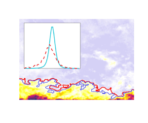
The statistics of spanwise vorticity for case C measured at  $X/M = 55$. (a) The j.p.d.f. of the spanwise vorticity and wall-normal location. (b) The normalised mean spanwise vorticity profile. (c) The vorticity distributions in the regions with $\Delta y/H \approx 5\,\%$ at the top and the bottom of the FOV, demarcated in (b), representing the freestream (the cyan lines) and boundary layer (the orange lines) vorticity distributions, respectively.

In our previous study (Asadi et al. Reference Asadi, Kamruzzaman and Hearst2022a), we highlighted the effect of incoming turbulence in manipulating the instantaneous momentum content of the core region of a turbulent channel flow, showing that when subjected to incoming turbulence, a constant velocity threshold could not correctly identify the core region in all PIV fields. This could be interpreted as a word of caution that employing a constant threshold value might not be the proper way to identify flow features in the presence of local variations in flow properties. This is not a new notion in investigating turbulent flows as the conventional way of identifying UMZs in TBLs is based on examining the instantaneous streamwise velocity histograms (e.g. Adrian et al. Reference Adrian, Meinhart and Tomkins2000; de Silva et al. Reference de Silva, Hutchins and Marusic2016). Nonetheless, since instantaneous data are more prone to noise and are limited by the spatial resolution as well as the extent of the domain, establishing a robust method to identify the flow features is a challenging task, especially in experimental studies.
The new method to identify the interface between a TBL and FST presented in this study is built upon the same physical basis identified by Wu et al. (Reference Wu, Wallace and Hickey2019a), i.e. that the TBL and FST contain different vortical structures. The TBL is directly affected by the presence of the wall and populated by hairpin vortices (Wu & Moin Reference Wu and Moin2009; Wu et al. Reference Wu, Moin, Wallace, Skarda, Lozano-Durán and Hickey2017), resulting in the dominance of prograde vortices, whose rotational direction is established by the mean shear. FST, however, contains random vortices originating from the interaction of the incoming flow and turbulence-producing objects, e.g. grid wings in the context of the current study. The mean spanwise vorticity profile for case C measured at  $X/M = 55$ is depicted in figure 3(b), where a strong negative mean spanwise vorticity is visible in the near-wall region, whose magnitude decays moving away from the wall. Figure 3(c) visualises the differences in the vortical organisation of the boundary layer and FST by illustrating the probability density function (p.d.f.) of vorticity in two regions at the top and the bottom of the PIV FOV (rectangular regions with $\Delta y/H \approx 5\,\%$ and $\Delta x$ equal to the entire extent of the FOV) for the same test case. As shown in this figure, the FST vorticity content has a symmetric distribution centred at zero, whereas the TBL vorticity distribution is clearly skewed towards negative values and is considerably wider than that in the FST region. It follows that an instantaneous field exhibits different vorticity distributions in the freestream and boundary layer regions.
Accordingly, beginning from the top regions of the FOV, the distribution of vorticity is assessed in different zones to identify the onset of the boundary layer region. Continuous contour lines of a constant property ( $\psi$) that span the entire extent of the FOV could be utilised to divide the PIV FOV into different regions of interest (ROIs). To determine whether a ROI belongs to the TBL or FST, its vorticity distribution is assessed. Two conditions are considered to identify the ROI as being a part of the instantaneous TBL: (1) the vorticity p.d.f. should be considerably different than that of local FST located above the ROI; at the same time, (2) the vorticity distribution in the ROI should have a clear tendency towards negative values. The first condition is examined by calculating the Euclidean distance between the p.d.f.s ( $D$) (functionally this is done with the pdist2 function in MATLAB), while the second condition is assessed using the median value, which is less sensitive to extreme outliers compared with the mean value.
The following steps were repeated for each instantaneous field to identify instantaneous interfaces.
(i) The highest continuous contour line of $\psi _a = \psi _{max}$ is identified in the instantaneous field.
(ii) The next continuous contour line located closer to the wall is identified for
$\psi _b = \psi _a - \Delta \psi$, demarcating a ROI confined between the two continuous contour lines of $\psi _a$ and $\psi _b$.(iii) The two conditions for the ROI to be identified as a part of the instantaneous TBL flow are: (1) the Euclidean distance between the ROI's vorticity p.d.f. and that of the local FST, located above the continuous contour line of
$\psi _a$, should be greater than a threshold value, i.e. $D > D_{th}$; (2) the median value of the ROI's vorticity distribution should be smaller than a negative threshold value, i.e. $M < M_{th}$.(iv) If both conditions are satisfied, the ROI is deemed to be a part of the instantaneous boundary layer flow. In this case, the top boundary marked by the continuous contour line of
$\psi _{th} = \psi _a$ is identified as the instantaneous interface.(v) Otherwise, the ROI is considered to belong to the FST, and the next ROI located closer to the wall is considered by setting
$\psi _a = \psi _b$ and repeating the procedure from step (ii).


Two different properties are utilised herein to divide the PIV FOV into different ROIs: streamwise velocity ( $\psi = u$) and spanwise vorticity magnitude ( $\psi = |\omega _z|$). The spacing of contour lines [step (ii)] should be carefully selected to be small enough to prevent missing the actual interface and at the same time, large enough to ensure an adequate number of data points within ROIs for reliable convergence of the spanwise vorticity p.d.f. and its median value. After careful inspection, the spacing was chosen as $\Delta u = 0.015U_\infty$ and $\Delta \omega _z = 0.075U_\infty /H$. In addition, in each iteration, the number of data points within the ROI was required to be greater than 800 for analysis reliability. If the condition was not met, that iteration would be skipped by setting $\psi _b = \psi _a - 2 \Delta \psi$. The requirement for a minimum number of data points constrains the proximity of two adjacent contour lines. In an idealised scenario where the contour lines are spaced uniformly in the wall-normal direction, this limit corresponds to approximately 2.5 mm for the current measurements (though such uniform spacing is seldom realised in practice). For the current dataset, this spacing ranges between 39 and 64 viscous units and from 1.6 % to 2.1 % of the boundary layer thickness $\delta$, representing the best and worst-case scenarios across all cases. It is important to note that this spacing is dictated largely by PIV resolution; thus, improvements in resolution could reduce the physical spacing further. As a result, the uncertainty in the detected interface is not inherent to the method itself but influenced by the measurement set-up; for example, the same technique applied to DNS would result in finer resolution. Furthermore, alternative criteria could be explored in the future to reduce the step size required for assessing differences in vorticity p.d.f.s.
Figure 4 shows a sample instantaneous field where the vorticity distributions are assessed for three different ROIs outlined using continuous contour lines of constant velocity. In this instantaneous field, ROI 1 is found to belong to the local FST flow as the vorticity distributions in local FST 1 and ROI 1 are very similar (figure 4c), hence neither of the two conditions in step (iii) are satisfied. Discrepancies between the vorticity distributions in local FST 2 and ROI 2 is observed (figure 4c); however, the vorticity distribution in ROI 2 exhibits no considerable tendency towards the negative vorticity values, i.e. the second condition in step (iii) is not satisfied. Moving to the next region closer to the wall, the spanwise vorticity p.d.f. in ROI 3 is skewed towards negative values and is significantly different from that in local FST 3 (figure 4i). Therefore, both conditions in step (iii) for ROI 3 to be a part of the boundary layer flow are met, and the red contour line is identified as the velocity interface in this particular instantaneous field.
An example of the interface identification procedure for an instantaneous velocity field of case C measured at  $X/M = 55$: (a), (d) and (g) instantaneous streamwise velocity field and (b), (e) and (h) instantaneous vorticity field for the first, second and third iteration of the interface detection procedure, respectively. The contour lines demarcate lines of constant velocity separating the local FST and the ROI. (c, f,i) Vorticity distributions inside the local FST (the cyan line) and the ROI (the orange dashed line) for the first, second and third iteration, respectively. The red line shows the continuous contour line of $u_{th} = 1.075U_\infty$ as the identified velocity interface for this instantaneous field.

The variations in vorticity distributions in the local FST for each test case are used to determine the two threshold values. For each instantaneous field, the vorticity median value in the region above the highest continuous velocity contour line was calculated, representing the median value of the vorticity distribution in the local FST flow ( $M_{i,FST}$ for $i = 1,2,\ldots, N$, where $N$ is the number of PIV samples for a test case). To keep the number of vorticity data points constant for the p.d.f. analysis, a rectangular region at the top of the FOV was used with $\Delta y/H \approx 5\,\%$ and $\Delta x$ equal to the entire extent of the interrogated domain, in which the variations of the vorticity p.d.f.s were quantified by calculating the Euclidean distance between each instantaneous p.d.f. and the mean p.d.f. ensemble averaged over the PIV fields of the test case ( $D_{i, FST}$ for $i = 1,2,\ldots, N$); to ensure the exclusion of any possible TBL regions from this quantification, the fields with the highest continuous velocity contour passing through the specified region were discarded. Subsequently, our inspections showed that threshold values of $D_{th} = 3 \sigma (D_{i,FST})$ and $M_{th} = 3 \sigma (M_{i,FST})$ could distinguish a TBL vorticity distribution from oscillations of the FST vorticity distribution. The sensitivity of the method to the threshold values is discussed in Appendix A. Instead of single vorticity data points, distributions of vorticity are utilised, resulting in greater robustness of the method to measurement noise.
Each instantaneous field is assigned a velocity threshold ( $u_{th}$) and a vorticity ( $|\omega _{th}|$) threshold, where the velocity and the vorticity interfaces are denoted by the continuous contour lines of the velocity threshold and the vorticity threshold, respectively. Although the instantaneous thresholds are identified for the majority of the fields, there are instances where no threshold could be identified. This occurs for an instantaneous field when no ROI satisfies both conditions on step (iii), and also, in some rare instances, when there is no continuous contour line of constant velocity or constant vorticity throughout the PIV FOV. The number of these instances depends on the streamwise extent of the FOV and the choice of $\psi$, and appears to increase with increasing FST intensity. Since it is common to identify UMZs over a streamwise extent of 2000 viscous units ( $\Delta x^+ = 2000$) using the velocity histogram method (Adrian et al. Reference Adrian, Meinhart and Tomkins2000; de Silva et al. Reference de Silva, Hutchins and Marusic2016; Hearst et al. Reference Hearst, de Silva, Dogan and Ganapathisubramani2021), to be consistent, a portion of each field in the centre of FOV with a streamwise extent of $\Delta x^+ = 2000$ is employed hereafter to identify interfaces, which are utilised later in § 4.4 to isolate the boundary layer flow and identify UMZs. In addition, the PIV fields with no identified interface, which form less than 3 % of the total fields for the worst case (most upstream position for case C), are left out of the analyses.
To address why two different contour lines, constant velocity contour lines and constant vorticity magnitude contour lines, are utilised to identify the interface between the TBL and FST, it is essential to consider the distinct roles they play in identifying turbulent events. Continuous contour lines of constant velocity were utilised in earlier studies to demarcate different momentum regions in turbulent flows, such as UMZs in turbulent wall-bounded flows (Adrian et al. Reference Adrian, Meinhart and Tomkins2000; de Silva et al. Reference de Silva, Hutchins and Marusic2016; Chen et al. Reference Chen, Chung and Wan2020; Gul et al. Reference Gul, Elsinga and Westerweel2020; Hearst et al. Reference Hearst, de Silva, Dogan and Ganapathisubramani2021), and the core region of turbulent channel flow (Kwon et al. Reference Kwon, Philip, de Silva, Hutchins and Monty2014; Yang et al. Reference Yang, Hwang and Sung2019; Asadi et al. Reference Asadi, Kamruzzaman and Hearst2022a). Constant vorticity contour lines are typically preferred for identifying TNTIs (Watanabe et al. Reference Watanabe, Zhang and Nagata2018). In the cases examined here, specifically for identifying UMZs within the TBL when subjected to FST, we find that constant velocity contour lines identify the UMZ region more clearly. This observation is explained here through the examination of two different sample instantaneous velocity fields, as depicted in figure 5. In the sample PIV field of case REF illustrated in figure 5(a–c), the red line represents the interface identified using a velocity contour line, whereas the green line is the selected vorticity interface. Notably, the velocity contour line effectively tracks the momentum events within the PIV field (figure 5a), whereas the vorticity contour line seems to bound the vortical features of the flow (figure 5c). Nevertheless, both interfaces identify the same UMZs within the TBL, as indicated by the modal peaks in the histogram of the streamwise velocity for the data points beneath the interfaces (figure 5d), with the UMZ edges (shown with blue lines in figure 5a,c) drawn at the midpoints between the two neighbouring modal velocities. Figure 5(e–h) shows similar figures for an instantaneous field of case C. While the velocity interface outlines the momentum events (figure 5d), the vorticity interface bounds the vortical features of the flow (figure 5g). However, the vorticity interface meanders through regions with severely different momentum content (figure 5f). As a result, it identifies an extra UMZ compared with the velocity interface (figure 5h). Moreover, as illustrated in figure 5( f), the vorticity magnitude based contour is incapable of providing an outer boundary for the UMZs within the field as it cuts through them. The examples provided in figure 5 are representative. Taking into account the insights of Dogan et al. (Reference Dogan, Hearst, Hanson and Ganapathisubramani2019), who argued that a TBL subjected to FST exhibits similarities to turbulent channel flow, and the findings of Kwon et al. (Reference Kwon, Philip, de Silva, Hutchins and Monty2014), Yang et al. (Reference Yang, Hwang and Sung2016, Reference Yang, Hwang and Sung2019) and Asadi et al. (Reference Asadi, Kamruzzaman and Hearst2022a), who highlighted the essential importance of the core region identified using constant velocity contour lines in turbulent channel flow dynamics, it is plausible that the interface between a TBL and FST identified using a velocity contour line harbours its own significance and should be considered in relevant analyses. Both the velocity and vorticity interfaces are identified and analysed in this study to further investigate their features; however, in § 4.4, the velocity interfaces are utilised to identify the UMZs within the TBL.
Two examples of instantaneous PIV fields with identified interfaces and UMZs. The instantaneous streamwise velocity fields are shown in (a) and (b) for the example of case REF and in (e) and ( f) for the example of case C. The red lines illustrate the velocity interface, whereas the vorticity interface is shown with the green lines. The instantaneous vorticity fields are shown in (c) and (g) for the example of case REF and case C, respectively. Histograms of the streamwise velocity beneath the velocity interface (red histograms) and the vorticity interface (green histograms) are presented in (d) and (h) for the example of case REF and case C, respectively. Blue symbols in (d) and (h) highlight the modal peaks in the histograms, corresponding to UMZs shown in (a), (b), (e) and ( f) with the UMZ edges (the blue lines) drawn at the midpoints between the two neighbouring modal velocities.

Figure 6(a,b) shows the distribution of velocity and vorticity thresholds, respectively, identified for case REF together with cases A, B and C measured at  $X/M = 55$. The eye is drawn immediately to the spread of both velocity and vorticity threshold values when FST is present. The former is in agreement with our previous observation in a turbulent channel flow affected by the incoming turbulence, where increasing the centreline turbulence intensity resulted in the spread of the distribution of modal velocities (see Asadi et al. Reference Asadi, Kamruzzaman and Hearst2022a, figure 5). Tables 4 and 5 list the mean and standard deviation of the identified velocity and vorticity thresholds, respectively, for all the test cases. The mean velocity and vorticity values, when different cases are compared, generally seems to slightly decrease and increase, respectively with increasing FST intensity. The standard deviations of both velocity and vorticity thresholds clearly increase with increasing FST intensities. A considerably wider spread of threshold values in the presence of FST emphasises the inadequacy of using a constant threshold value to identify the interface in these flows with high FST levels. However, this approach may still be effective in identifying the interface in low-turbulence freestream flows, as indicated by the narrow distribution of velocity and vorticity thresholds observed in case REF. The fact that the FST and REF cases differ in this way is a key finding, illustrating the need for dynamic thresholding. The efficacy of this approach is demonstrated in subsequent sections.
Distributions of the normalised threshold values. (a,b) Distributions of the velocity thresholds and the vorticity thresholds, respectively, identified for cases A (blue), B (green) and C (red) measured at  $X/M = 55$ as well as REF (grey). (c) Distributions of both the velocity thresholds (——) and vorticity thresholds ( $-\bullet -$) identified for case B at the different streamwise locations, with the lighter colours indicating the increased streamwise distance from the grid.

The mean and standard deviation of the velocity thresholds and the corresponding interface location, as well as the UMZ statistics for the cases at the different streamwise locations.

The mean and standard deviation of the vorticity thresholds and the corresponding interface location.

Having identified the interfaces, it is now possible to examine the effect of FST on the intermittency of the TBL and the spatial location of the interface. Mean intermittency ( $\gamma$) profiles are calculated by binarising the velocity grid points according to their position in each instantaneous field, i.e. the grid points between the interface and the bottom wall are located inside the TBL and are given a value of 1, whereas the grid points above the interface are considered to be a part of FST and their value is set to zero. Ensemble averaging of the binarised values across the PIV fields and then in the streamwise direction yields the intermittency profile. Figure 7(a) illustrates the intermittency profiles for case REF together with that of Reuther & Kähler (Reference Reuther and Kähler2018) and Borrell & Jiménez (Reference Borrell and Jiménez2016) for TBLs, where the TNTIs were identified using the local seeding method in experimental measurements and a vorticity threshold ( $|\omega |^* = 0.2$) in DNS, respectively. The wall-normal location is normalised using $\delta _{99}$ to make the profiles comparable. When comparing the intermittency profiles of case REF obtained using the velocity and vorticity interfaces, it is observed that the latter exhibits slightly lower and higher intermittency values in the regions with $0.5< y/\delta _{99}<0.8$ and $1< y/\delta _{99}<1.2$, respectively. This might be linked to a more contorted vorticity interface in the PIV fields. The intermittency profile of the vorticity interface shows a closer agreement with those found in other studies. Furthermore, the mean and standard deviation of the interface location ( $\kern0.7pt \overline {y_i}$ and $\sigma (y_i)$, respectively) listed in tables 4 and 5 are well within the range of the previous TNTI studies (see e.g. Borrell & Jiménez Reference Borrell and Jiménez2016, figure 4).
(a) Intermittency profiles for case  $|\omega ^*| = 0.2$ from Borrell & Jiménez (Reference Borrell and Jiménez2016) ( $-\blacktriangleleft -$, black), case $s_{th} = 40$ from Reuther & Kähler (Reference Reuther and Kähler2018) ( $\circ$, violet) and case REF of the present study obtained using the velocity interface ( $-\blacklozenge -$, grey) and the vorticity interface ( $-\blacksquare -$, grey). (b,d) Intermittency profiles and (c,e) p.d.f.s of the interface location for cases A (blue), B (green) and C (red) measured at $X/M = 55$ as well as case REF (grey), with (b,c) derived using the velocity interfaces and (d,e) derived using the vorticity interfaces.

Figure 7(b,c) depict the intermittency profiles and p.d.f.s of  $y_i$, respectively, derived using the momentum interface for case REF and active cases measured at $X/M = 55$. The same profiles for the vorticity interface are shown in figure 7(d,e). The figures clearly show notable disparities in the spatial characteristics of the interface for the REF case compared with the active cases. For the REF case, $\gamma$ and the $y_i$ p.d.f. can be approximated as Gaussian, which aligns with the findings of previous studies (Chauhan et al. Reference Chauhan, Philip, de Silva, Hutchins and Marusic2014; Borrell & Jiménez Reference Borrell and Jiménez2016). However, this Gaussian approximation does not hold true for cases A, B and C. Considering these active cases in figure 7(c,e), there are visible differences between the p.d.f.s in the inner regions, where the peak moves closer to the wall for increased FST intensities, suggesting that on average the increased FST intensity pushes the interface closer to the wall. The $\overline {y_i}$ values listed in tables 4 and 5 confirm this notion, which is also consistent with previous observations indicating that increased incoming flow turbulence pushed the uppermost UMZ edge of a ZPG-TBL, and the core boundary of a turbulent channel flow closer to the wall (Hearst et al. Reference Hearst, de Silva, Dogan and Ganapathisubramani2021 and Asadi et al. Reference Asadi, Kamruzzaman and Hearst2022a, respectively). In addition, similar to the results of the latter regarding increased variations in the core boundary location, the $\sigma (y_i)$ values, listed in tables 4 and 5, increase when subjected to increased FST fluctuations. It is worth mentioning that in figure 7(c,e) the $y_i$ distributions for the active cases are very similar in the regions close to the top of the FOV, indicating the bounding effect of free surface, which, in turn, seems to suppress the increase in $\delta$ by FST, as was listed explicitly in table 3.
While the velocity and vorticity interfaces exhibit similarities in terms of the statistical properties of their spatial characteristics, the distinct characteristics of these interfaces become evident in their ability to highlight relevant phenomena. As illustrated in figure 5, the velocity interface captures momentum-related events within the TBL, whereas the vorticity interface emphasises vortical features. This distinction underscores the need to consider both types of interfaces for a comprehensive understanding of TBL dynamics. We also acknowledge that the vorticity magnitude used herein is derived from the spanwise vorticity. For the specific case of a TNTI, the total vorticity magnitude or enstrophy are typically employed via DNS. While these quantities are disproportionately governed by the spanwise vorticity near the wall (by orders of magnitude) they are not necessarily perfectly analogous to it and, thus, their instantaneous contours may differ. This is a topic for future DNS studies to investigate while integrating the variable thresholding presented herein. In addition, both the total vorticity magnitude and the enstrophy are unsigned quantities, limiting a key criterion used to differentiate the freestream from the boundary layer, i.e. the sign of the spanwise vorticity. Thus, in the subsequent section, we delve deeper into the specific insights provided by the velocity and vorticity interfaces, elucidating their respective roles in characterising turbulent flow structures and dynamics.
4. Streamwise evolution
Using pointwise measurements, Jooss et al. (Reference Jooss, Li, Bracchi and Hearst2021) pioneered the investigation of the streamwise evolution of a TBL affected by FST. They found that the spatial development of a TBL and FST is an essential determinant of the TBL state under FST influence. Performing PIV measurements at four different streamwise locations, i.e.  $X/M = 55$, 65, 72 and 85, along with the new method to identify the instantaneous interfaces, enables us to examine the streamwise evolution of the interface characteristics and how this affects the organisation of UMZs in the boundary layer. The active cases measured at $X/M = 55$ are compared with case REF to highlight the FST effects; nevertheless, the observed trends are applicable to the active cases measured at the other streamwise locations.
4.1. Intermittency and the interface location
As shown in figure 6(a,b), increasing the FST intensity resulted in increased variations of the velocity and vorticity thresholds identified to mark the interface. The distributions of the velocity and vorticity thresholds for case B at different streamwise locations are depicted in figure 6(c). P.d.f.s of the velocity thresholds, represented by the solid lines in the figure, exhibit a sharper peak and a narrower distribution by moving in the streamwise direction, i.e. the lighter colours. A more condensed range of vorticity thresholds is also noticed in this figure, where, generally, there is a decline in the likelihood of finding high vorticity threshold values as one moves in the streamwise direction. As the intensity of FST decreases farther downstream from the grid, the trends observed in figure 6(c) suggest a resurgence of the threshold distribution shown in figure 6(a,b) for REF. The same trend is also confirmed for all three cases (not shown here). This observation is significant in that it demonstrates that the effect of the turbulence is not to affect a permanent change on the TBL that is transported downstream but rather is local.
The effects of FST on the intermittency and the location of the interfaces were discussed in § 3. The  $\overline {y_i}$ values increases in the streamwise direction for each active case (tables 4 and 5), indicating the movement of the interface away from the wall. Although the trend in the fluctuations is less clear, $\sigma (y_i)/\overline {y_i}$ tangibly decreases moving in the streamwise direction. This is different than what was observed by You & Zaki (Reference You and Zaki2019) for the material boundary of the TBL, where the $\sigma (y_i)/\overline {y_i}$ value increased abruptly after a sudden injection of homogeneous-isotropic turbulence on top of the TBL and then remained constant farther downstream. The progressively more chaotic behaviour of the interface observed by You & Zaki (Reference You and Zaki2019) might be attributable to the artificial addition of FST in their DNS and/or the way the boundary layer fluid was tracked in their work by ignoring the entrainment process. Overall, the interface statistics presented in the current study, similar to the velocity and vorticity threshold distributions, show a return to the undisturbed state.
Figure 8 shows the streamwise evolution of the intermittency and  $y_i$ distribution obtained using the velocity and vorticity interfaces for cases A, B and C. The REF case is also included for comparison. The wall-normal coordinate is normalised by $\overline {y_i}$ for each test case as it provides a more physical scaling basis compared with $\delta$ which solely depends on the mean velocity profile. Moving in the streamwise direction, the intermittency increases in the inner regions, corresponding to the movement of the interface away from the wall. This is also visualised in figure 8(g–l), where the peaks of the p.d.f.s are located farther from the wall for downstream measurement locations, i.e. lighter colours. As shown by case REF, for a Gaussian distribution of $y_i$, the peak is located at $y/y_i = 1$, and $\gamma = 0.5$ at $y/y_i = 1$. The streamwise trends in the profiles are in the same direction, where the peak location moves away from the wall and the intermittency grows at $y/y_i = 1$. Thus, similar to the velocity thresholds, a tendency to recover the canonical characteristics is observed when moving downstream of the active grid.
Streamwise evolution of (a–f) intermittency profiles and (g–l) p.d.f.s of the interface location for cases A (blue), B (green) and C (red) in the left, the middle and the right panels, respectively, with lighter colours indicating increased streamwise distance from the grid. (a–c) and (g–h) are derived using the velocity interfaces, whereas (d–f) and (j–l) are for the vorticity interfaces.

4.2. Conditional averages
Conditional averaging is a common tool in boundary layer studies to examine flow statistics in the vicinity of an interface, e.g. TNTIs (Chauhan et al. Reference Chauhan, Philip, de Silva, Hutchins and Marusic2014; Eisma et al. Reference Eisma, Westerweel, Ooms and Elsinga2015), UMZs (de Silva et al. Reference de Silva, Philip, Hutchins and Marusic2017; Chen et al. Reference Chen, Chung and Wan2020), the core boundary of turbulent channel flow (Kwon et al. Reference Kwon, Philip, de Silva, Hutchins and Monty2014; Yang et al. Reference Yang, Hwang and Sung2016; Asadi et al. Reference Asadi, Kamruzzaman and Hearst2022a) and the boundary of a ZPG-TBL subjected to FST (Wu et al. Reference Wu, Wallace and Hickey2019a; Hearst et al. Reference Hearst, de Silva, Dogan and Ganapathisubramani2021). The same technique is employed here to probe the flow statistics in the proximity of the identified interfaces. A local wall-normal coordinate is defined whose origin is always on the interface, i.e.  $y-y_i$. This allows us to move along the interface and average the statistics towards the boundary layer and FST, i.e. $y-y_i < 0$ and $y-y_i>0$, respectively. The conditionally averaged profiles are then calculated by averaging the vertical profiles over the instantaneous PIV fields for each test case. A prerequisite for this analysis is that the interface should be a single-valued function of $x$. This is not always the case since the interface folds back on itself occasionally. To circumvent the issue, whenever the interface takes on several wall-normal locations at a specific $x$, the closest point to the wall is chosen as the interface location for the velocity interface, ensuring that no FST is included as a boundary layer region in the analysis. For the vorticity interface, the farthest point from the wall is selected, representing the projection of the freestream on to the interface. Hereafter, the conditional averaging is denoted by angle brackets, i.e. $\langle \,\rangle$.
Figure 9 shows the conditionally averaged profiles derived using the velocity and vorticity interfaces for the active cases measured at the most upstream measurement location, i.e.  $X/M = 55$. The results of the REF case are also included for comparison. Figure 10(a) demonstrates the conditionally averaged streamwise velocity profiles. The profiles are offset by the mean conditional velocity at the interface location ( $\langle u_i \rangle$). The conditionally averaged profiles across both the velocity and the vorticity interface show a relatively uniform streamwise velocity inside the FST and a positive shear within the TBL in all the cases. The transition between these regions is different for the velocity and vorticity interfaces. When considering the velocity interfaces, a sharp jump in the streamwise velocity profile occurs across the interface, where the magnitude of the jump increases with increasing FST intensity. This is consistent with the observations of Hearst et al. (Reference Hearst, de Silva, Dogan and Ganapathisubramani2021) and Asadi et al. (Reference Asadi, Kamruzzaman and Hearst2022a). Using the approach utilised by Chauhan et al. (Reference Chauhan, Philip, de Silva, Hutchins and Marusic2014) and Hearst et al. (Reference Hearst, de Silva, Dogan and Ganapathisubramani2021) to quantify the magnitude of the jump ( $D[U_\infty ]$) for the conditionally averaged profiles across the velocity interface shown in figure 9(a) yields $D[U_\infty ] \approx 0.03$, 0.05, 0.06 and 0.07 for REF, A, B and C, respectively. In contrast, a smooth transition links the uniform velocity profile on the freestream side of the vorticity interface to the sheared velocity profile on the TBL side, and there is thus no explicit velocity jump across the vorticity interface.
(a) Streamwise velocity, (b) spanwise vorticity and (c) streamwise turbulent fluctuations profiles conditionally averaged across the velocity interface (——) and the vorticity interface ( $-\bullet -$) for cases A (blue), B (green) and C (red) measured at $X/M = 55$ as well as case REF (grey).

Streamwise evolution of (a–c) streamwise velocity, (d–f) spanwise vorticity and (g–i) streamwise turbulent fluctuations profiles conditionally averaged across the velocity interface (——) and the vorticity interface ( $-\bullet -$) for cases A (blue), B (green) and C (red) in the left, the middle and the right panels, respectively, with lighter colours indicating increased streamwise distance from the grid.

Figure 9(b) presents the conditionally averaged spanwise vorticity profiles. It is clear that the mean spanwise vorticity level inside the TBL is negative, whereas it is zero in the freestream. This is true for both the velocity and vorticity interfaces and provides strong evidence for the validity of the method, which was supposed to identify an interface separating the vortical structures of the TBL from those of the FST. The previously observed difference in the behaviour of the conditionally averaged velocity profiles is also represented here, where sharp peaks in the vorticity profiles are indicative of high shear events at the velocity interface, similar to the previous observations for TNTIs (Chauhan et al. Reference Chauhan, Philip, de Silva, Hutchins and Marusic2014; Eisma et al. Reference Eisma, Westerweel, Ooms and Elsinga2015), the uppermost UMZ edge of a TBL subjected to FST (Hearst et al. Reference Hearst, de Silva, Dogan and Ganapathisubramani2021) and the core boundary of turbulent channel flows (Kwon et al. Reference Kwon, Philip, de Silva, Hutchins and Monty2014; Asadi et al. Reference Asadi, Kamruzzaman and Hearst2022a), while the sharp jumps of the mean vorticity are observed across the vorticity interface similar to the previous observation for TNTI identified using a spanwise vorticity threshold (Borrell & Jiménez Reference Borrell and Jiménez2016; Watanabe et al. Reference Watanabe, Zhang and Nagata2018).
The streamwise fluctuations are evaluated with respect to the conditionally averaged velocity profiles, and the resulting streamwise-normal Reynolds stress profiles are shown in figure 9(c). A relatively uniform fluctuation level is exhibited within the freestream, whereas the fluctuations increase on the TBL side of the interface when moving towards the wall, i.e.  $(y-y_i)<0$. The bulge in the profiles obtained using the velocity interface is an artefact of using constant velocity contour lines in instantaneous velocity fields and were similarly visible in the results of Chauhan et al. (Reference Chauhan, Philip, de Silva, Hutchins and Marusic2014) (see figure 6 in their work), who used a constant KED threshold to identify the TNTI.
The results presented above exhibit the characteristics expected from an interface that separates the FST region with a uniform mean velocity and negligible mean spanwise vorticity from the TBL region with a sheared velocity profile and mean negative spanwise vorticity, affirming the validity of the method. It should be noted that the physical characteristics of the conditionally averaged properties have been taken into account in this study to confirm the validity of the method. This provides a more vigorous standard than the conventional logic of merely observing step changes in the conditional statistics (see Appendix B for an example).
To assess the streamwise evolution of the conditionally averaged properties, the profiles measured at different streamwise locations are depicted in figure 10 for each grid case, i.e. case A, B and C in the left, the middle and the right column, respectively. To avoid inclusion of the streamwise changes in the normalisation of the vertical coordinate, it is normalised by  $H$, which is a constant. When considering the profiles obtained using the velocity interface, a similar streamwise trend is observed for all the tested cases, where the magnitude of the streamwise velocity jump across the the velocity interface decreases in the streamwise direction (figure 10a–c); consequently, the peaks in the conditionally averaged vorticity profiles appear to generally diminish downstream of the grid. On the boundary layer side of the interface, the mean spanwise vorticity magnitude drops by moving farther downstream, whereas on the freestream side, it retains an approximately zero value regardless of the streamwise location (figure 10d–f). The former can be explained by the movement of the interface away from the wall, and the latter is an inherent feature of the freestream as discussed earlier. Moreover, figure 10(g–i) exhibit similar trends as seen in figure 9(c), where the level of streamwise fluctuations scales with the FST intensity and thus diminishes downstream of the grid. The trends observed in the profiles acquired using the vorticity interface are generally similar to those found using the velocity interface, where the streamwise velocity profiles in figure 10(a–c) display reduced shear within the TBL when moving downstream of the grid. This corresponds to a decrease in mean vorticity magnitude on the TBL side of the profiles in figure 10(d–f). The uniformity of the velocity and the absence of vorticity within the FST remain consistent in all examined scenarios at various streamwise positions. The only deviation is in the scaling of the streamwise velocity fluctuations conditionally averaged across the vorticity interface, where no meaningful pattern is seen. This indicates that the vorticity interface does not accurately track the momentum events in the fields when FST is present, as shown explicitly in figure 5( f) for a specific field. Overall, when considering the streamwise development of conditionally averaged profiles, a similar recovery effect is observed, with the statistics tending to return to the conditional averages across the interface as seen in case REF.
4.3. Zonal averages
In boundary layer studies, zonal averaging is utilised to investigate the differences between the flow features when the flow is situated inside different regions at different wall-normal locations. For example, the wall-normal profiles of flow statistics were examined by Kwon et al. (Reference Kwon, Philip, de Silva, Hutchins and Monty2014) inside and outside the core region of a turbulent channel flow, Chen et al. (Reference Chen, Chung and Wan2020) inside different UMZs of a turbulent pipe flow and You & Zaki (Reference You and Zaki2019) inside and outside the material boundary of a TBL subjected to FST. We employ the same technique here to examine the streamwise velocity statistics zonally averaged inside the TBL and FST. The details of the technique were described by You & Zaki (Reference You and Zaki2019) (see § 3.1 of their work entitled ‘conditional sampling’). In short, the same binary values used for calculating the intermittency profiles are used here as a weighting factor to calculate the zonal averages inside the TBL and FST.
The streamwise velocity profiles zonally averaged inside the boundary layer ( $U_{BL}$) and freestream ( $U_{FS}$) for REF together with active cases at $X/M = 55$ are depicted in figure 11(a,d) derived using the velocity and the vorticity interfaces, respectively. It should be noted that $U_{BL}$ and $U_{FS}$ can be combined using $\gamma$ to reproduce the mean velocity profile, i.e. $U = \gamma U_{BL} + (1-\gamma ) U_{FS}$. The zonally averaged profiles of the active cases inside FST are only shown for the regions with $\gamma < 0.9$ since FST is seldom present beyond this range. The same is applied to the zonally averaged TBL profiles for the regions with $\gamma > 0.1$. In both figure 11(a) and 11(d), the boundary layer profiles are matched in the log region for the different cases and closely follow the logarithmic law of the wall, whereas the wake suppression effect by increasing the FST level is visible in the outer region. In fact, the wake suppression effect induced by FST results from a combination of a more frequent presence of freestream flow in the regions closer to the wall (as shown in figure 7) and a fuller $U_{BL}$ profile. When demarcated by the velocity interface, the freestream exhibits a more uniform streamwise velocity level (figure 11a) than when demarcated by the vorticity interface (figure 11a). Figure 11(b,e) illustrates zonally averaged fluctuations of streamwise velocity relative to the zonal mean obtained using the velocity and the vorticity interface, respectively. The boundary layer profiles in the inner regions follow the general scaling trend observed in figure 2(b), indicating amplification of turbulent fluctuations within the boundary layer by FST. In figure 11(b), freestream fluctuation profiles maintain a constant level in the wall-normal direction, whereas in figure 11(b), elevated fluctuation levels are observed within the freestream in the inner regions. The spanwise vorticity profiles zonally averaged inside the TBL and FST are illustrated in figure 11(c, f) derived using the velocity and the vorticity interface, respectively. The vorticity interface ensures a consistent zero mean vorticity level within the FST independent of the wall-normal location, whereas the zonally averaged profiles in the FST, obtained from the velocity interface, show non-zero vorticity levels in the inner areas. The results presented in figure 11 elucidate the underlying difference between the velocity and the vorticity interface in distinguishing the freestream flow from the TBL based on the momentum and the vorticity content, respectively, demonstrating the validity of the method.
Profiles of (a) and (d) the inner normalised mean velocity, (b) and (e) streamwise turbulent fluctuations and (c) and ( f) spanwise vorticity zonally averaged inside the boundary layer (the solid lines as well as the lines with filled symbols) and FST (the dashed lines as well as the lines with open symbols) for cases A (blue), B (green) and C (red) measured at  $X/M = 55$ as well as case REF (grey). (a–c) are derived using the velocity interface, whereas (d–f) are derived using the vorticity interface.

The streamwise development of the zonally averaged statistics obtained using the velocity and the vorticity interface are illustrated in figures 12 and 13, respectively, for cases A, B and C. The inner normalised velocity profiles (figures 12a–c and 13a–c) illustrate a gradual recovery of the wake region with the decay of FST intensity in the streamwise direction, as noted before in the mean velocity profiles shown in figure 2(a) and similar to the results of Jooss et al. (Reference Jooss, Li, Bracchi and Hearst2021). The log region remains intact at various streamwise locations, corroborating the robustness of the logarithmic law of the wall to freestream perturbations, as previously illustrated in figure 2(a) and observed in other studies (Hancock & Bradshaw Reference Hancock and Bradshaw1989; Dogan et al. Reference Dogan, Hanson and Ganapathisubramani2016; Hearst et al. Reference Hearst, Dogan and Ganapathisubramani2018; You & Zaki Reference You and Zaki2019; Jooss et al. Reference Jooss, Li, Bracchi and Hearst2021). The FST fluctuation profiles in figures 12(d–f) and 13(d–f) are arranged in a decreasing order moving in the streamwise direction, indicating the decay of the grid generated turbulence. For cases A and B, the boundary layer fluctuation profiles collapse in the inner regions for different streamwise locations, whereas the FST intensity level separates them in the outer regions. In case C, however, the FST impact on the boundary layer profiles in the outer regions extends closer to the wall, indicating a deeper penetration of the FST effects on the streamwise fluctuations of the boundary layer in this case with a significant level of turbulence in the freestream. This distinction is similar to the findings of Jooss et al. (Reference Jooss, Li, Bracchi and Hearst2021) (see figure 5e, f in their paper). The spanwise vorticity profiles zonally averaged inside the FST, depicted in figures 12(g–i) and 13(g–i), generally collapse, indicating that the streamwise development has no impact on the FST profiles. The TBL profiles exhibit minor deviations for  $y/\delta <0.5$, where the vorticity magnitude decreases slightly when moving in the streamwise direction. The TBL profiles generally match for $y/\delta >0.5$, indicating an outer scaling of the vorticity in this region.
Streamwise evolution of (a–c) the inner normalised mean velocity, (d–f) streamwise turbulent fluctuations and (g–i) spanwise vorticity profiles zonally averaged inside the boundary layer (the solid lines) and FST (the dashed lines) obtained using the velocity interfaces for cases A (blue), B (green) and C (red) in the left, the middle and the right panels, respectively, with lighter colours indicating increased streamwise distance from the grid.

Streamwise evolution of (a–c) the inner normalised mean velocity, (d–f) streamwise turbulent fluctuations and (g–i) spanwise vorticity profiles zonally averaged inside the boundary layer (the lines with filled symbols) and FST (the lines with open symbols) obtained using the vorticity interfaces for cases A (blue), B (green) and C (red) in the left, the middle and the right panels, respectively, with lighter colours indicating increased streamwise distance from the grid.

4.4. UMZs
The existence of UMZs in TBLs exposed to FST was confirmed by Hearst et al. (Reference Hearst, de Silva, Dogan and Ganapathisubramani2021). Given the observations of Jooss et al. (Reference Jooss, Li, Bracchi and Hearst2021) that streamwise evolution also plays a role in the system, it is natural to wonder how the UMZs evolve in space. Hearst et al. (Reference Hearst, de Silva, Dogan and Ganapathisubramani2021) identified the UMZs using the well-established histogram method, in which the instantaneous freestream flow was eliminated in the histogram analysis to avoid concealing the peaks corresponding to the UMZs characteristic velocities (see figure 18 in their work). Following in the footsteps of de Silva et al. (Reference de Silva, Hutchins and Marusic2016) and Laskari et al. (Reference Laskari, de Kat, Hearst and Ganapathisubramani2018), Hearst et al. (Reference Hearst, de Silva, Dogan and Ganapathisubramani2021) identified a KED-based interface as the uppermost UMZ edge of the TBL and disregarded the flow above the interface. The same histogram-based technique is employed here to identify the UMZs, where the instantaneous interfaces identified using the velocity contour lines are employed to separate the TBL flow from FST. As illustrated in the examples of figure 5, the velocity interfaces effectively isolate the momentum events associated with the TBL, which, in turn, allows for the correct identification of the UMZs present in the TBL. Apart from using the new method to identify the instantaneous boundary layer flow, the other steps are the same as stated by Hearst et al. (Reference Hearst, de Silva, Dogan and Ganapathisubramani2021) in section 4.2 of their paper. As mentioned earlier in § 3, a subdomain of the PIV FOV in the centre with a streamwise extent of  $\Delta x^+ = 2000$ is chosen for the analysis. The instantaneous streamwise velocity is isolated below the momentum-based interface whose histogram (with a bin size of $0.1U_\infty$) is examined to identify the peaks as the modal velocities of the UMZs ( $u_{{UMZ}}$). The midpoint between the two neighbouring modal velocities can then be used to mark the boundary between the two adjacent UMZs. The peak detection parameters, i.e. peak prominence, peak height and minimum peak distance, are optimised to ignore spurious peaks in the histograms and kept the same for the different test cases. Although varying the streamwise domain extent, histogram bin size and peak detection parameters affects the number of the detected UMZs ( $N_{{UMZ}}$), the observed trends when comparing the test cases with each other are found to be robust and similar to what was found by Hearst et al. (Reference Hearst, de Silva, Dogan and Ganapathisubramani2021). Figure 14 illustrates examples of the instantaneous fields with the identified UMZs for cases B and C measured at $X/M = 55$ as well as REF.
Examples of PIV fields with identified UMZs and their modal velocities. (a), (c), and (e) are the instantaneous PIV fields of case REF, case B measured at  $X/M = 55$ and case C measured at $X/M = 55$, respectively, with the red lines indicating the velocity interface between the boundary layer and the freestream, and the blue lines indicating the UMZ edges within the boundary layer. (b), (d), and ( f) show the p.d.f. of the normalised instantaneous streamwise velocity within the boundary layer for case REF, case B measured at $X/M = 55$ and case C measured at $X/M = 55$, respectively, with the red symbols indicating the identified modal velocities of the UMZs.

The average number of identified UMZs ( $\overline {N_{{UMZ}}}$) is presented in table 4 for all the test cases. Comparing REF with the active cases, similar to the results of Hearst et al. (Reference Hearst, de Silva, Dogan and Ganapathisubramani2021), fewer UMZs are identified when the TBL is influenced by FST. The fields in figure 14 are chosen to illustrate the general trends observed in the presence of FST, where the velocity interface approaches the wall and the number of identified UMZs decreases. According to Hearst et al. (Reference Hearst, de Silva, Dogan and Ganapathisubramani2021), one possible explanation would be the destruction of the UMZs in the boundary layer by FST whenever its fluctuations are comparable to those in the boundary layer at a particular wall-normal location. On the other hand, the underlying dynamics of the flow inside the boundary layer are observed to be robust to FST perturbations (Dogan et al. Reference Dogan, Hanson and Ganapathisubramani2016, Reference Dogan, Hearst and Ganapathisubramani2017; Hearst et al. Reference Hearst, Dogan and Ganapathisubramani2018), and as discussed in § 4.2, the flow characteristics inside the boundary layer were only subjected to a level change that appeared to be mainly due to the variations of the interface position. Accordingly, this might suggest that the UMZs are compressed closer to the wall and masked due to the limited spatial resolution of PIV in the near-wall region. In fact, this hypothesis is in line with the observation made by de Silva et al. (Reference de Silva, Hutchins and Marusic2016) that the instantaneous location of the TNTI did not affect the number of the UMZs present in the boundary layer; instead, when the interface was situated farther from the wall, the upper UMZs in the boundary layer were thicker. If the inner UMZs are compressed, occasionally a portion of them might be discernible in the measurement domain. In that case, it is likely that the upper boundary of the UMZ is discontinuous, i.e. the contour line marking the upper edge of the UMZ does not span the whole extent of the FOV. An example is illustrated in figure 15 for a sample PIV field of case C measured at $X/M = 55$, where the black contour lines marking the upper edge of the UMZ closer to the wall are discontinuous and reach the bottom of the FOV. The occurrence rate of these fields ( $R_{d}$) containing discontinuous UMZs is listed in table 4 as a percentage of the total examined fields.
(a) A sample instantaneous PIV field of case C measured at  $X/M = 55$, with the red line indicating the velocity interface between the boundary layer and FST, and the black lines marking the discontinuous boundary between the UMZs. (b) The histogram of the normalised instantaneous streamwise velocity within the boundary layer, with the red symbols indicating the identified modal velocities of the UMZs.

Furthermore, table 4 lists the average number of the continuous UMZs ( $\overline {N_{{UMZ,c}}}$) calculated by discarding the discontinuous UMZs. As presented for case REF, less than 1 % of the PIV fields contain a discontinuous UMZ, indicating that almost all the UMZs in the PIV fields were large enough for the current spatial resolution to fully cover their upper edge. Thus, discarding the discontinuous UMZs does not considerably affect the average number of the identified UMZs for this case. In contrast, $R_{d}$ increases significantly when the TBL is subjected to increasing FST intensities. Consequently, when discarding the discontinuous UMZs, $\overline {N_{{UMZ}}}$ noticeably decreases for the active cases. It should be mentioned that discontinuous UMZs are always detected in proximity to the bottom edge of the FOV, where the UMZ boundary extends all the way down. In conclusion, when FST is present, a frequent presence of UMZ segments near the bottom of the examined domain indicates the compression of the UMZs in this region. This also implies information is buried in the regions closer to the wall due to low spatial resolution, especially given the fact that the separation of the scales should be larger for a higher turbulent state. Nonetheless, further investigation of the structures in the near-wall region requires higher spatial resolution in the near-wall region or is better suited for DNS investigations. To ensure consistency when comparing cases, the discontinuous UMZs are neglected in the remainder of the present study.
Figure 16(a) illustrates the distribution of  $N_{{UMZ,c}}$ identified in the PIV fields of the active cases measured at $X/M = 55$ as well as REF. When FST is present, the number of PIV fields with $N_{{UMZ,c}} \geq 2$ is still greater than those with $N_{{UMZ,c}} = 1$, indicating the existence of UMZs within the TBL for the cases tested in this study. In the presence of FST, the number of instantaneous fields with more than two UMZs in the boundary layer is significantly reduced, and the p.d.f.s exhibit a peak at $N_{{UMZ,c}} = 2$. The former is similar to the trend observed by Hearst et al. (Reference Hearst, de Silva, Dogan and Ganapathisubramani2021) in figure 11(a) of their work. $\overline {N_{{UMZ,c}}}$ (listed in table 4) for the active cases measured at the same streamwise location demonstrates a decreasing trend as FST intensity increases. Figure 16(b) depicts the p.d.f.s of the modal velocities for the same cases as shown in 16(a). Among the active cases, the change in the distribution of the modal peaks is more noticeable than the variations of $N_{{UMZ,c}}$. Artificial peaks were observed by Hearst et al. (Reference Hearst, de Silva, Dogan and Ganapathisubramani2021) in the distribution of modal velocities in figure 11(b) (figure 11b in Hearst et al. Reference Hearst, de Silva, Dogan and Ganapathisubramani2021 has a mislabelled $x$-axis: their figure 11b shows the same information as figure 16b of the present work, i.e. the p.d.f. of the UMZ modal velocities) of their work caused by the constant KED threshold used to separate the instantaneous TBL and FST flows; since individual threshold values are selected in this study for this purpose, no spurious peaks are observed in figure 16(b). In fact, similar to the p.d.f.s of the threshold values shown in figure 6(a), the modal peaks are more evenly distributed for increased FST intensities. A greater spread in the distribution of the modal velocities with a higher FST intensity is similar to what we observed (Asadi et al. Reference Asadi, Kamruzzaman and Hearst2022a, figure 5) for modal peaks in a turbulent channel flow affected by inlet turbulence. This is a direct effect of the increased variations of the streamwise momentum inside the boundary layer induced by FST (see figure 11b). In addition, figure 16(b) shows that the probability of the occurrence of the UMZs with $u_{{UMZ}} > U_\infty$ significantly increases in the presence of FST. Based on the analysis of Heisel et al. (Reference Heisel, De Silva, Hutchins, Marusic and Guala2020), who showed that the mean velocity profile could be derived by averaging UMZ velocities, the fuller $U_{BL}$ profiles in the presence of FST, as discussed in § 4.3, can be attributed to the more frequent occurrence of UMZs with higher characteristic velocities.
The distribution of the (a) number of continuous UMZs and (b) normalised modal velocities identified for the active cases measured at  $X/M = 55$ as well as REF: REF, $-\blacklozenge -$, grey; case A, $-\blacksquare -$, blue; case B, $-\bullet -$, green; case C, $-\blacktriangle -$, red.

Figure 17 shows the streamwise changes in the distribution of  $N_{{UMZ,c}}$ and $u_{{UMZ}}$ for cases A, B and C. In general, moving in the streamwise direction, the occurrence of PIV fields with $N_{{UMZ,c}} = 1$ decreases, whereas the number of fields in which two or more UMZs are identified increases. An increasing trend is observed for $\overline {N_{{UMZ,c}}}$ with development of the flow in the streamwise direction (see table 4). This indicates that as the interface moves away from the wall with the decay of FST in the streamwise direction, more continuous UMZs are identified throughout the examined domain. The p.d.f.s of $u_{{UMZ}}$ measured at different streamwise locations (figure 17d–f) appear to change in accordance with the FST intensity, especially for $u_{{UMZ}}/U_\infty > 0.8$, where generally the peak in the p.d.f. grows sharper, whereas the probability of $u_{{UMZ}}/U_\infty > 1$ decreases with decreasing FST intensities in the streamwise direction. Overall, the UMZs within the TBL exhibit the same recovery pattern observed for the other TBL properties.
Streamwise evolution of the distributions of (a–c) number of continuous UMZs and (d–f) normalised modal velocities for case A ( $-\blacksquare -$, blue), case B ( $-\bullet -$, green) and case C ( $-\blacktriangle -$, red), respectively, with lighter colours indicating increased streamwise distance from the grid.

5. Conclusion and discussion
Planar PIV measurements were performed to examine the effects of FST on the instantaneous structure of a TBL and how these effects evolve in the streamwise direction. Three different active grid sequences were utilised to produce FST cases with different turbulence intensities, which were tested at four different streamwise locations downstream of the grid. A reference case with significantly lower FST content was tested as well.
A new method has been introduced to identify the interface between the instantaneous TBL and FST flows. The regions of the flow were marked using continuous contour lines, with the fields analysed twice: once using velocity contour lines and once using vorticity contour lines to identify both a velocity interface and a vorticity interface. Two criteria were employed to distinguish the local FST from a region within the boundary layer adjacent to it: (1) the vorticity p.d.f.s should be considerably different; (2) in the boundary layer region, the median value of the vorticity distribution should be notably negative. As a result, individual velocity and vorticity thresholds have been determined for each instantaneous field, and the interfaces have been marked by continuous contour lines of constant velocity and vorticity thresholds.
The spatial characteristics of the interface were significantly altered by FST, regardless of the chosen interface (velocity or vorticity). Notably, the p.d.f. of the interface location for the active cases could not be described by a normal Gaussian distribution, unlike that for case REF. Furthermore, in the presence of FST, the interface moves considerably towards the wall. Certain distinctions in the flow characteristics near the interface were elucidated by conditional averaging for the velocity interface when compared with the vorticity interface, where the velocity interface exhibited a sharp jump in the streamwise velocity and a sharp peak in the spanwise vorticity at the interface location, whereas a smooth transition of the streamwise velocity and a sharp jump in the spanwise vorticity were observed at the vorticity interface location. Nevertheless, the trends with increased FST intensity were similar, where increased magnitudes of the shear and spanwise vorticity were observed within the TBL with increasing FST intensity. In addition, the overall shape of the conditionally averaged profiles for the velocity or the vorticity interface did not change when the TBL was subjected to various incoming FST intensities, indicating the robustness of the flow dynamics inside the TBL. Moreover, on the freestream side of the interface, a uniform mean velocity and negligible mean vorticity were found for all the tested cases, as expected for grid-generated turbulence. The zonally averaged profiles inside the FST revealed that the mean velocity and streamwise fluctuations were more uniform when the velocity interface was used; on the other hand, the vorticity interface produced more uniform vorticity profiles. This highlighted the different behaviour of the velocity interface and vorticity interface in outlining the momentum events and the vortical features of the flow, respectively. Note, such clear differences were not necessarily apparent from previous TNTI studies where both the momentum and vorticity isocontours roughly separate rotational from irrotational fluid, although specifics along the lines may differ. Nonetheless, the zonally averaged profiles obtained using both interfaces showed the robustness of the log region as well as a wake suppression effect and increased TBL fluctuations for the active cases. The velocity interface was used to isolate the TBL for identifying the UMZs as it was demonstrated that the vorticity interface cuts through the UMZs whereas the momentum interface caps them. Under the influence of FST, the average number of identified UMZs in the boundary layer decreased, whereas the occurrence of UMZs in the near-wall region with discontinuous boundaries increased. This indicated compression of the UMZs closer to the wall as a result of the interface moving towards the wall. The streamwise evolution of the effects was investigated for each of the active cases by comparing the statistics measured at different locations downstream of the grid. In line with the previous observations of Jooss et al. (Reference Jooss, Li, Bracchi and Hearst2021), a general recovery of the statistics was observed when moving downstream away from the turbulence generating grid, regardless of the interface choice. This included the displacement of the interface average location away from the wall and a decrease in the velocity/vorticity jump across the interface. Downstream of the grid, the turbulent fluctuations within the freestream diminished, resulting in a weakening of the effects on the zonal averages within the boundary layer, i.e. the return of the wake and a reduction in streamwise turbulent fluctuations. Moving in the streamwise direction, the number of the identified UMZs with continuous boundaries appeared to increase.
This study marks a significant step forwards by elucidating the features of the velocity interface and the vorticity interface between a TBL and FST. It is crucial to consider the unique significance of each interface in relevant analysis. The velocity interface employed in this study is well-suited for examining the characteristics of UMZs within the TBL, similar to the established method of using a velocity interface to demarcate the boundary of the quiescent core in turbulent channel flows. Meanwhile, the vorticity interface may be more suitable for investigating vorticity transport events within these flows. The layer between rotational and irrotational fluid provides more flexibility in the analysis as it is home to isolines of momentum, vorticity and passive scalars, although these are not necessarily all perfectly colocated. However, when considering two turbulent flows, these quantities represent distinct phenomena due to the differences in their transport equations in fully turbulent flows. Therefore, it is imperative to only use a specific interface to track phenomena relevant to that interface, for instance, misleading results might be produced by studying momentum events using a vorticity interface or vice versa. Such results should be considered in future studies attempting to define a universal ‘turbulent–turbulent interface’ separating different regions of turbulence, should such a phenomenon exist. The present results demonstrate that understanding and respecting the unique features and roles of each interface is essential for accurate analysis and interpretation of TBL dynamics under varying incoming flow conditions. Furthermore, this study has identified, for the first time, how the instantaneous structure of a TBL evolving beneath FST changes in space.
Acknowledgement
The authors are grateful to Prof. J. Westerweel for detailed information and insightful discussion on single-pixel PIV processing.
Funding
This project and all authors were funded by the Research Council of Norway (RCN) project number 288046 (WallMix). Later stages of RJH's work were support by the European Union through a ERC Starting Grant (GLITR, 101041000). Views and opinions expressed are however those of the authors only and do not necessarily reflect those of the European Union or the European Research Council Executive Agency. Neither the European Union nor the granting authority can be held responsible for them.
Declaration of interests
The authors report no conflict of interest.
Data availability statement
The velocity vector fields for all test cases examined in this study are publicly accessible through DataverseNO at doi:10.18710/MVG1OX.
Appendix A. Sensitivity analysis of the interface detection method
As stated in § 3, two threshold values were utilised to assess the differences between the vorticity distributions in the local freestream and ROIs. The thresholds were defined based on the variations of the vorticity distributions in freestream regions, i.e.  $D_{th} = 3\sigma (D_{i,FST})$ and $M_{th} = 3\sigma (M_{i,FST})$. Varying these threshold values affects the selected $u_{th}$ and $|\omega _{th}|$ in some of the PIV fields. A sensitivity analysis is carried out by increasing and decreasing the reference threshold values, i.e. $D_{th} = 3\sigma (D_{i,FST})$ and $M_{th} = 3\sigma (M_{i,FST})$, by 10 %, 25 % and 50 % to examine the effect on the results. Figure 18 shows the velocity interface location statistics for different threshold values. The results are presented for the active cases measured at $X/M = 55$, case C measured at different streamwise locations, as well as REF, which represents the general patterns across all test cases. Minor variations in the reference threshold values, e.g. $\pm$10 %, do not significantly affect the statistics. The results for case REF demonstrate a higher degree of robustness to more severe changes in the threshold values due to the significantly lower vorticity content in the freestream. In addition, for the active cases, the changes in $\overline {y_i}$ values are more notable than $\sigma (y_i)$. In general, when the threshold values are increased, lower velocity contour lines, i.e. those that are closer to the wall, are chosen as the interface in some of the fields, resulting in lower $\overline {y_i}$ values. The opposite is observed for decreased threshold values. Nevertheless, when comparing the cases with each other, the trends discussed in §§ 3 and 4.1 are valid regardless of the selected threshold values. The same trends were also observed for the vorticity interface (not shown here), independent of the chosen threshold values.
The mean (the filled symbols) and standard deviation (the open symbols) of the interface location vs threshold values for (a) case A ( $-\blacksquare -$, blue), case B ( $-\bullet -$, green) and case C ( $-\blacktriangle -$, red) measured at $X/M = 55$ as well as REF ( $-\blacklozenge -$, grey), and (b) case C ( $-\blacktriangle -$, red) measured at different streamwise locations with lighter colours indicating increased streamwise distance from the grid. The reference threshold values are $D_{th} = 3\sigma (D_{i,FST})$ and $M_{th} = 3\sigma (M_{i,FST})$ for each test case.

To investigate the effects on the conditional averages, figure 19 illustrates the conditionally averaged profiles of the streamwise velocity and the spanwise vorticity derived using the velocity and the vorticity interface for various threshold values. For better visualisation, only the most turbulent case, i.e. case C measured at  ${X/M = 55}$, is shown as a representative of all test cases. As shown, the deviations of the profiles are negligible for small changes in the reference threshold values ( $\pm$10 %). However, a substantial increase in the reference threshold values, e.g. $+$50 %, biases the interface towards the boundary layer region in some of the fields; consequently, increased magnitudes of the mean shear and spanwise vorticity are observed on the FST side of the interface, i.e. $(y-y_i) > 0$. In contrast, when the reference thresholds are significantly decreased, for instance by $-$50 %, the interface is shifted towards the freestream in certain PIV fields. This, in turn, causes decreased magnitudes of the mean shear and vorticity on the boundary layer side of the interface. Similar to what was observed for the interface location statistics, the trends for the conditionally averaged profiles and the other properties discussed in § 4 are found to be robust to the variations of the threshold values for both the velocity and the vorticity interface (not shown here for brevity). Overall, the sensitivity analysis underlines the idea expressed by Borrell & Jiménez (Reference Borrell and Jiménez2016) and Wu et al. (Reference Wu, Wallace and Hickey2019a) that the thresholds represent ranges of values as opposed to specific values.
(a,c) Streamwise velocity and (b,d) spanwise vorticity profiles conditionally averaged across the interface for case C measured at  $X/M = 55$. (a) and (b) are derived using the velocity interface, whereas (c) and (d) are for the vorticity interface. The interface is identified by applying $-$50 %, $-$25 %, $-$10 %, $+$10 %, $+$25 % and $+$50 % change (the grey lines with darkening colours, respectively) to both $D_{th} = 3 \times \sigma (D_{i,FST})$ and $M_{th} = 3 \times \sigma (M_{i,FST})$ used in this study (the red lines).

It is worth mentioning that the bin size of the vorticity p.d.f.s, i.e.  $2$ s
$2$ s $^{-1}$, was chosen based on the evaluated uncertainties (see § 2.2). The sensitivity of the results to this parameter is also assessed (not shown here), and the statistics are found to be robust to minor increases/decreases in the value. However, a significant increase in the bin size (more than 25 %) masks the differences between the vorticity distributions in the boundary layer and freestream regions, posing severe issues for the identification process.
Appendix B. Comparison of the method with the KED approach
It is worth comparing the method proposed in this study to identify the velocity interface between a TBL and FST with the KED method utilised by de Silva et al. (Reference de Silva, Hutchins and Marusic2016), Laskari et al. (Reference Laskari, de Kat, Hearst and Ganapathisubramani2018) and Hearst et al. (Reference Hearst, de Silva, Dogan and Ganapathisubramani2021) to identify the uppermost UMZ edge in their TBLs. As a representation of all the test cases, the results are shown for the test case with the highest FST intensity, i.e. case C measured at  $X/M = 55$. The method used by Hearst et al. (Reference Hearst, de Silva, Dogan and Ganapathisubramani2021) is utilised to determine the constant KED threshold ( $k_{th}$), which yields the greatest proportion of PIV fields with a continuous KED contour (see § 4.1 of their work for details of the method). As shown in figure 20(a), a normalised threshold value of $k_{th}/k_\infty = 1.2$ is identified ( $k_\infty$ denotes the mean KED value in the freestream region), resulting in continuous KED contours in approximately 88 % of the total PIV fields. The interface location statistics calculated using the KED approach are $\overline {y_i} = 51.0$ mm and $\sigma (y_i) = 42.2$ mm, resulting in $\sigma (y_i)/\overline {y_i} = 0.829$, compared with $\overline {y_i} = 56.6$ mm, $\sigma (y_i) = 40.9$ mm, and $\sigma (y_i)/\overline {y_i} = 0.72$ evaluated by the newly introduced method for the velocity interfaces. Figure 20(b,c) depict the streamwise velocity and spanwise vorticity fields, respectively, for a sample PIV field of case C measured at $X/M = 55$, as well as the interfaces identified by both methods. Figure 20(d) illustrates the vorticity distributions in the region between the interfaces (the orange dashed line) and in the local freestream region (the solid cyan line). As shown, the vorticity distribution in the region between the two contour lines is considerably different than that in the local freestream and clearly skewed towards negative values, indicating that this region belongs to the instantaneous boundary layer. This indicates that the boundary between the instantaneous TBL and FST is more precisely delineated by the vorticity-based method. Although this field is an example, it represents the general concept that using the KED approach with a single threshold value cannot differentiate between the vortical structures of the TBL and those of the FST. This is further investigated here by examining the conditional averages. Figure 21 illustrates the conditionally averaged flow properties across the velocity interfaces quantified using the method introduced in this work and the KED approach. In the freestream region, the conditionally averaged profiles diverge noticeably. The KED approach shows a significant shear with increasing streamwise velocities inside the freestream (figure 21a) that is uncharacteristic of the freestream. Although the interface selected by the KED method leads to a step change in the conditionally averaged vorticity profile (figure 21b), the mean vorticity magnitude inside the freestream is non-zero, indicating incorrect interface choices typically biased towards the boundary layer side of the interface.
(a) Percentage of PIV fields in which a continuous KED contour exists at  $k_{th}$ for case C measured at $X/M = 55$; the grey dashed line indicates the selected threshold. (b,c) An instantaneous streamwise velocity and spanwise vorticity field, respectively, of case C measured at $X/M = 55$. The interfaces identified using the vorticity-based method ( $u_{th} = 1.005\,U_\infty$) and the KED approach ( $k_{th}/k_\infty = 1.2$) are indicated with the red and blue lines, respectively. (d) The vorticity distributions in the regions above the higher interface, i.e. local FST region (the cyan line), and between the interfaces (the orange dashed line).

(a) Streamwise velocity and (b) spanwise vorticity profiles conditionally averaged across the velocity interface identified using the current method (the solid red lines) and the KED method (the dashed black lines) for case C measured at  $X/M = 55$.

Based on the aforementioned evidence, a single KED threshold has insufficient precision in the presence of FST and results in blurred statistics. Furthermore, the conditionally averaged statistics shown in figure 21 should be regarded as a warning that a mere step change in the statistics across the interface without exhibiting any consistent physical characteristics should not be interpreted as confirmation that correct interfaces between various regions in the flow have been identified.


 Open access