


Introduction
Sediment cores retrieved from paleolakes provide valuable records of past climatic conditions, and in the eastern African rift (EAR) these can be linked directly to the environments in which our hominin ancestors evolved. Retrieved cores are subjected to a myriad of tests, some quick and nondestructive (e.g., geophysical scans, imaging, and core-scan X-ray fluorescence [XRF]), and others that require more time-consuming and destructive sampling, sample preparation, and laboratory analysis (e.g., X-ray diffraction [XRD], isotopic analyses, biomarker analyses, and paleomagnetic and radiometric age dating). By necessity these sample-based studies will also have a coarser resolution than the scans, yielding records on the decimeter to meter scale depending on sampling interval compared with continuous or centimeter-scale resolution of the various imaging and scanning techniques. This results in two difficulties: (1) while the labor-intensive sample-based data (e.g., XRD mineralogy) yield more readily interpretable paleoclimate proxies, which can be linked more directly to changes in aridity or lake conditions, the coarser sampling resolution can result in missed shorter-duration events; and (2) while scans (e.g., XRF elemental abundances) might pick up on shorter-duration events and more accurately place major transitions, deciphering the causes of such changes based on scan data alone can be challenging.
To address this issue, Kodikara et al. (Reference Kodikara, McHenry, Stanistreet, Stollhofen, Njau, Toth and Schick2024) developed a wide and deep learning model to predict the relative mineral compositions of sediment cores based on XRF scan data. They used the 1-cm-resolution core-scan XRF data from the 2014 Olduvai Gorge Coring Project (OGCP) Cores 2A and 3A, retrieved from the Pleistocene Olduvai basin in northern Tanzania (Stanistreet et al., Reference Stanistreet, Boyle, Stollhofen, Deocampo, Deino, McHenry, Toth, Schick and Njau2020a), in conjunction with the XRD-derived mineral assemblages from the same cores determined for samples collected at 32 cm intervals within fluviolacustrine units (McHenry et al., Reference McHenry, Kodikara, Stanistreet, Stollhofen, Njau, Schick and Toth2020a). Their deep learning models were able to predict the presence of minerals and whether they were abundant or trace with high accuracies.
The current study will (1) apply the trained deep learning model (from Kodikara et al., Reference Kodikara, McHenry, Stanistreet, Stollhofen, Njau, Toth and Schick2024) to the entire OGCP Cores 2A and 3A to predict mineral assemblages at 1 cm intervals throughout the finer fluviolacustrine intervals; and (2) validate these predictions against published XRD data, sedimentological core descriptions, and core images. We will evaluate the predictive capabilities of the model for each mineral class based on XRD data and core descriptions, identify potential causes of discrepancies along with strategies for improvement, and propose recommendations for future methodological improvements.
Background
The Olduvai basin is a rift-shoulder basin associated with the EAR in northern Tanzania (Fig. 1), which hosted an often saline-alkaline lake for much of the Pleistocene. Olduvai Gorge cuts through the sedimentary record exposing lake, lake margin, alluvial fan/plain, volcanic, and volcaniclastic deposits in outcrop (Hay, Reference Hay1976). The stratigraphy exposed by Olduvai Gorge is subdivided into a series of beds, from oldest to youngest: Beds I–IV, Masek, Ndutu, and Naisiusiu (Hay, Reference Hay1976). These outcrops also expose a world-renowned record of hominin evolution, including fossils of multiple hominin species, associated lithic artifacts, and related faunal remains (Leakey, Reference Leakey1971), some of which include cut marks left by stone tools (e.g., Pante et al., Reference Pante, Blumenschine, Capaldo and Scott2012). The volcanic record exposed by the gorge documents the explosive eruptive history of the adjacent Ngorongoro Volcanic Highlands (NVH) (e.g., Hay, Reference Hay1976; McHenry et al., Reference McHenry, Mollel and Swisher2008). Evidence from outcrop shows that Paleolake Olduvai expanded and contracted over time, following both long-term trends toward increased aridity and shorter-term, often cyclical wet–dry cycles (e.g., Hay, Reference Hay1976; Ashley, Reference Ashley2007; Deocampo et al., Reference Deocampo, Berry, Beverly, Ashley and Jarrett2017; Stanistreet et al., Reference Stanistreet, Boyle, Stollhofen, Deocampo, Deino, McHenry, Toth, Schick and Njau2020a).
Location of the Olduvai basin and positions of the 2014 Olduvai Gorge Coring Project (OGCP) cores. (A) Map of East Africa. (B) Regional map showing the geographic context of Olduvai Gorge on the shoulder of the eastern African Rift (EAR), with the Ngorongoro Volcanic Highlands (NVH) to the east and south and metamorphic basement exposures to the west and north (map after Ashley and Hay, Reference Ashley, Hay, Renaut and Ashley2002). (C) Map of the Olduvai basin, showing the locations of Olduvai Gorge, major faults, the reconstructed position of the Olduvai paleolake during the deposition of Beds I and II, and the position of the three 2014 OGCP coring locations (map after Stanistreet et al., Reference Stanistreet, Boyle, Stollhofen, Deocampo, Deino, McHenry, Toth, Schick and Njau2020a).

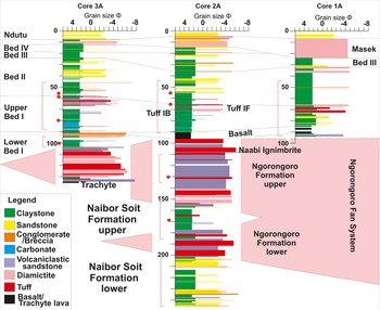
The gorge only exposes a small part of the basin’s sedimentary record, both in terms of area and depth. To capture a more complete record, in 2014 the OGCP retrieved four sediment cores (1A, 2A, 3A, and 3B) from three different locations, targeting the anticipated depocenter for the paleolake at various times (originally designated by Hay [Reference Hay1976], revised in Stollhofen and Stanistreet [Reference Stollhofen and Stanistreet2012]). These provide an excellent record of the Olduvai paleolake and show that it was older, deeper, and more continually present than expected based on analysis of outcrop stratigraphy (Stanistreet et al., Reference Stanistreet, Stollhofen, Deino, McHenry, Toth, Schick and Njau2020b). A map of the Olduvai basin, incorporating the revised extent of its depocenter during deposition of Beds I and II in the Pleistocene based on OGCP results, is presented in Figure 1C. The older part of the record, exposed in Core 3A and especially in Core 2A (which extends to 245 m below the surface, with ∼135 m of section below the stratigraphic level known from outcrop), comprises the newly defined Ngorongoro (volcanic) and Naibor Soit (fluviolacustrine) Formations (Stanistreet et al., Reference Stanistreet, Stollhofen, Deino, McHenry, Toth, Schick and Njau2020b). The base of Core 2A, dating to ∼2.3 Ma (Deino et al., Reference Deino, Heli, King, McHenry, Stanistreet, Stollhofen, Njau, Mwankunda, Schick and Toth2021), still lies within fluviolacustrine sediments. Figure 2 shows detailed stratigraphy for Cores 2A and 3A after Stanistreet et al. (Reference Stanistreet, Stollhofen, Deino, McHenry, Toth, Schick and Njau2020b). More details on these cores are available in the following papers: introduction/overview: Njau et al. (Reference Njau, Toth, Schick, Stanistreet, McHenry and Stollhofen2021); stratigraphy/sedimentology: Stanistreet et al. (Reference Stanistreet, Stollhofen, Deino, McHenry, Toth, Schick and Njau2020b); geochronology: Deino et al. (Reference Deino, Heli, King, McHenry, Stanistreet, Stollhofen, Njau, Mwankunda, Schick and Toth2021); tephrostratigraphy: McHenry et al. (Reference McHenry, Stanistreet, Stollhofen, Njau, Schick and Toth2020b); and carbonates: Stanistreet et al. (Reference Stanistreet, Doyle, Hughes, Rushworth, Stollhofen, Toth, Schick and Njau2020c). Of particular relevance to the current study are McHenry et al. (Reference McHenry, Kodikara, Stanistreet, Stollhofen, Njau, Schick and Toth2020a): paleolake mineralogy using XRD; and Stanistreet et al. (Reference Stanistreet, Boyle, Stollhofen, Deocampo, Deino, McHenry, Toth, Schick and Njau2020a): core-scan XRF.
Stratigraphic sections for Olduvai Gorge Coring Project (OGCP) Cores 1A, 2A, and 3A. Beds I and II and the top of the Ngorongoro Formation have outcrop equivalents, while most of the Ngorongoro Formation and all of the Naibor Soit Formation are known only from these cores. The intervals for which X-ray diffraction (XRD) data are available in McHenry et al. (Reference McHenry, Stanistreet, Stollhofen, Njau, Schick and Toth2020b) are indicated with red brackets. The representative sections discussed at length in this paper are indicated with red dots.

McHenry et al. (Reference McHenry, Kodikara, Stanistreet, Stollhofen, Njau, Schick and Toth2020a) report XRD-derived relative mineral abundances for the finer-grained (fluviolacustrine) intervals of the OGCP cores, sampled at 32 cm intervals, from 45 m below surface (mbs) to the bases of Cores 1A, 2A, and 3A, for a total of 426 samples. These data show changes in mineralogy over time in the Olduvai paleolake, including changes in sediment source (e.g., more detrital quartz from western fluvial sources in younger intervals, more volcanic anorthoclase in older intervals sourced from the NVH to the east) and the changing salinity, alkalinity, and composition of the lake (e.g., different zeolite minerals, authigenic K-feldspar, clay minerals, and carbonates).
Stanistreet et al. (Reference Stanistreet, Boyle, Stollhofen, Deocampo, Deino, McHenry, Toth, Schick and Njau2020a) used intensity counts and element ratios from core-scan XRF data from Cores 2A and 3A (from ∼1.3 to 2.0 Ma) to show high-resolution changes in elemental composition, focusing on Mg, Al, and Ti. Following prior work by Deocampo et al. (Reference Deocampo, Berry, Beverly, Ashley and Jarrett2017), Mg served as a proxy for authigenic clays, while elevated Al and Ti were interpreted to indicate more detrital input. Especially in upper Olduvai Bed I and lower Bed II, these proxies showed robust cyclical trends, interpreted as alternating wet and dry cycles associated with precession, obliquity, or shorter-duration events, and following similar trends reconstructed using other proxies, including carbon isotopes and biomarkers (Colcord et al., Reference Colcord, Shilling, Sauer, Freeman, Njau, Stanistreet, Stollhofen, Schick, Toth and Brassell2018, Reference Colcord, Shilling, Freeman, Njau, Stanistreet, Stollhofen, Schick, Toth and Brassell2019; Shilling et al., Reference Shilling, Colcord, Karty, Hansen, Freeman, Njau and Stanistreet2019, Reference Shilling, Colcord, Karty, Hansen, Freeman, Njau and Stanistreet2020). Similar trends were also identified in the XRD-derived mineral assemblages reported in McHenry et al. (Reference McHenry, Gebregiorgis and Foerster2023), where the presence, absence, and relative abundance of zeolite minerals and authigenic K-feldspar also appear to track wet–dry cycles for this interval.
The deep learning model developed by Kodikara et al. (Reference Kodikara, McHenry, Stanistreet, Stollhofen, Njau, Toth and Schick2024) for the 2014 OGCP cores used the Keras deep learning framework (https://keras.io) and consists of two sub-models: a classification model and a regression model. The classification model is used to predict the mineral assemblages (likely presence or absence of specific minerals or mineral groups), while the regression model predicts the relative abundances of mineral groups. The models were created using the sequential class and functional application programming interfaces with different wide and deep neural network architectures. Wide and deep neural networks provide the benefits of both memorization and generalization of input data for prediction, which is particularly relevant in interpretative fields such as geology. The model was trained using 1329 samples, which consist of core-scan XRF elemental intensity data from Stanistreet et al. (Reference Stanistreet, Boyle, Stollhofen, Deocampo, Deino, McHenry, Toth, Schick and Njau2020a), along with lithology derived from detailed core descriptions from Stanistreet et al. (Reference Stanistreet, Stollhofen, Deino, McHenry, Toth, Schick and Njau2020b). The mineralogy data for those samples were obtained from the XRD-derived mineral assemblages reported by McHenry et al. (Reference McHenry, Kodikara, Stanistreet, Stollhofen, Njau, Schick and Toth2020a). The models were built by first defining the input features as element ratios derived from XRF scan intensity data. Selected element intensity ratios were transformed to log scales to avoid artifacts generated by possible dilution effects. Correlation matrices were calculated for these element ratios to quantify the strength of association between pairs of element ratios in the dataset. After careful analysis of the correlations between each element ratio pair as well as mineral presence in the dataset, and based on the literature, geochemical reasoning, and prioritizing elements with related geochemical behavior, 12 element ratios were selected: K/Al, Ca/Al, Mg/Al, Fe/Al, K/Si, Ca/Si, Mg/Si, Fe/Si, Si/Al, S/Fe, Mg/Ca, and Ca/K. These cover the elements that constitute the major (non-accessory) mineral phases identified in this study.
The final dataset for the model developed in Kodikara et al. (Reference Kodikara, McHenry, Stanistreet, Stollhofen, Njau, Toth and Schick2024) includes the core-scan XRF intensity values of seven elements (Al, Ca, Fe, K, Mg, S, and Si), the lithology of each sample position (based on detailed core descriptions, subdividing samples into claystone, clay-sand, sandstone, tuff, carbonate, or diamictite categories), and the mineral abundances at each sample location based on qualitative analysis of XRD data (where relative abundance was estimated as abundant, common, minor, trace, or absent based on relative peak height in McHenry et al. [Reference McHenry, Kodikara, Stanistreet, Stollhofen, Njau, Schick and Toth2020a]). No semiquantitative estimated mineral abundances were available for this dataset, but the qualitative estimates are expected to be internally consistent. The dataset was split into training, validation, and testing sets to ensure generalization and prevent overfitting. Training involved iterating over various architectures and hyperparameters such as learning rates, computational model layer structures, and computational model activation functions. The validation dataset was used to select the best-performing configurations. The model was validated using 265 unseen data records, and its accuracy was assessed with six additional test records. The optimized deep neural network (DNN) achieved greater than 86% binary accuracy, while the regression models demonstrated high reliability in predicting the relative mineral abundances of the samples. Improvements were made by analyzing model loss and accuracy trends to mitigate overfitting and enhance predictive power.
Methods
The current study uses the previously described trained deep learning models to reconstruct the mineral assemblages of two OGCP cores (Cores 2A and 3A) at 1 cm intervals, an improvement over the 32 cm interval of XRD sampling of the lacustrine intervals. Details of data preparation, feature engineering, the selection of DNN models, hyperparameter tuning, and model accuracies of the trained models can be found in Kodikara et al. (Reference Kodikara, McHenry, Stanistreet, Stollhofen, Njau, Toth and Schick2024). The dataset for this study consists of core-scan XRF intensities for seven elements (Al, Ca, Fe, K, Mg, S, and Si) from Stanistreet et al. (Reference Stanistreet, Doyle, Hughes, Rushworth, Stollhofen, Toth, Schick and Njau2020c) along with the lithology descriptions of each sample point (Supplementary Tables S1–S4). Six lithological classes were selected: carbonate (includes carbonates and marl), sandy clay (includes clayey sandstone), claystone, diamictites (mudflow), sandstone, and tuff (which includes reworked tuff/volcaniclastic sandstone). Coarse-grained lithological classes such as conglomerate and breccia, along with samples that fell on lithological boundaries (referred to as “ambiguous” in McHenry et al. [Reference McHenry, Kodikara, Stanistreet, Stollhofen, Njau, Schick and Toth2020a]) were excluded from this study, because the original models were not trained to classify these categories and no XRD data are available for the coarser lithologies for comparison. The process and justification for the selection of these element ratios and grouped lithology classes for the model are discussed in detail in Kodikara et al. (Reference Kodikara, McHenry, Stanistreet, Stollhofen, Njau, Toth and Schick2024). The models were run on a FreeBSD 14.1 desktop computer (AMD Phenom 6-core at 2.799 GHz, 20 GB RAM, GT 710 GPU) using the neovim text editor.
Results
The trained model can predict the mineral assemblages (presence/absence of minerals or mineral groups) and their relative abundances using regression and classification models, respectively. For classification models, mineral assemblages were categorized into classes based on lithological context and geochemical associations, allowing for binary predictions of mineral presence. The classification model can predict 10 mineral or mineral groups: quartz, plagioclase, K-feldspar, calcite, dolomite, non-analcime zeolites, analcime, smectite, illite, and Fe-bearing minerals. The probabilities of the presence of these minerals were rescaled to 0–1. We recommend a threshold of 0.5 to determine mineral presence, balancing sensitivity and specificity. However, because it is difficult to assign one common threshold value for all lithologies for all cores, we present the original probability values for more qualitative interpretations. Minerals with a score of 0.5 or higher are considered likely present. The detailed results of our classification models for Cores 2A and 3A, along with the core-scan XRF intensities for the elements used, lithologies, and XRD-derived mineral assemblages from McHenry et al. (Reference McHenry, Kodikara, Stanistreet, Stollhofen, Njau, Schick and Toth2020a), are presented in Supplementary Tables 1 and 2.
The regression modeling results predict abundances for five mineral classes: quartz, feldspars (K-feldspar and plagioclase, considered together), carbonates (calcite, dolomite, and aragonite, considered together), zeolites (including analcime and others), and clay minerals (both smectite and illite). The mineral group abundances derived from the regression model were scaled between 0 and 1, with individual values reflecting relative rather than absolute proportions. It is important to note that these values do not sum to 1, as they represent independent estimates of each mineral’s relative abundance (and more than one mineral can be “abundant” in a single sample). The predicted mineral assemblages and abundances of those mineral groups for Cores 2A and 3A, along with the core-scan XRF intensities for the elements used, lithologies, and XRD-derived mineral assemblages from McHenry et al. (Reference McHenry, Kodikara, Stanistreet, Stollhofen, Njau, Schick and Toth2020a) are presented in Supplementary Tables 3 and 4.
Although the deep learning models were applied to the entirety of Cores 2A and 3A (that contained the modeled lithologies), specific ∼3 m intervals of interest were selected for more detailed discussion, due to (1) the availability of 32-cm-resolution XRD data; (2) the presence of previously identified mineralogical transitions based on the XRD data; (3) coverage of different intervals of the paleolake record; and (4) correspondence to intervals of interest in Olduvai Gorge outcrops (e.g., boundary of Beds I and II, directly above Tuff IF). For these intervals, the model-generated mineral assemblages with their relative abundances were compared with the core descriptions (lithology), core images, and individual XRD patterns and resulting XRD-derived mineral assemblages.
Discussion
The detailed sedimentological descriptions (Stanistreet et al., Reference Stanistreet, Stollhofen, Deino, McHenry, Toth, Schick and Njau2020b) and extensive published database of XRD-derived mineral assemblages (McHenry et al., Reference McHenry, Kodikara, Stanistreet, Stollhofen, Njau, Schick and Toth2020a) make the 2014 OGCP cores an excellent test case for whether mineral assemblages can be satisfactorily predicted based on core-scan XRF elemental data. The following examples are representative cases, including intervals and lithologies for which the models performed well (consistent with XRD-based mineral assemblages and core descriptions) and others where the model struggled to re-create the previously documented assemblages. The example core intervals are presented in stratigraphic order, from youngest to oldest.
Olduvai Bed II paleolake, Cores 2A and 3A
Core 2A: 2A-23Y-(1-2), 54–56.8 mbs
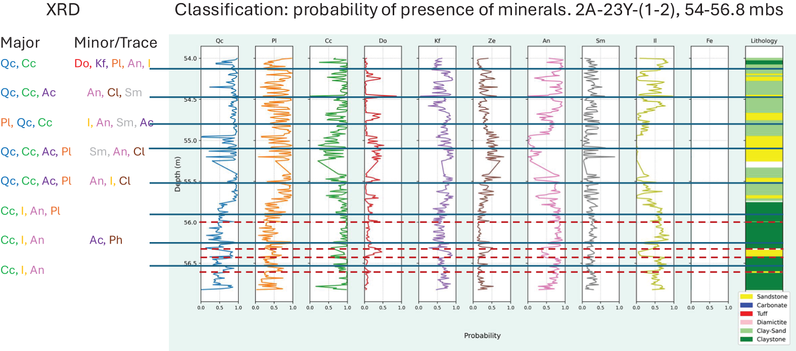
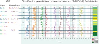
This interval was selected to represent Olduvai Bed II and covers an interval that transitions from claystone-dominated to sandstone-dominated, with intervals of both throughout. Based on the XRD results published in McHenry et al. (Reference McHenry, Kodikara, Stanistreet, Stollhofen, Njau, Schick and Toth2020a), it also covers a major mineralogical shift, with quartz not observed below 55.6 mbs but ubiquitous above. Calcite and analcime are recognized in all XRD samples from this interval. For the samples with the strongest clay signals in their bulk XRD patterns, illite is the dominant clay (although smectite is also observed as a trace phase in some samples).
The classification model for this interval (Fig. 3) shows a change in the probability of quartz at ∼55.7 mbs. Below this level, the probability of quartz is under 0.5 for about half of the data points (but notably higher in the two thin sandstone layers within this interval), while above that level it is predicted to be present in almost every sample. Analcime is predicted to be present in almost all samples except those in the thicker sandstone. Where clays are predicted (most intervals excluding sandstone), illite is much more likely than smectite. The probability for calcite is high for much of this interval, with dolomite reaching 0.5 for only a few “spikes” that do not correspond to XRD-sampled intervals.
Classification model results for core interval 2A-23Y-(1-2), 54–56.8 m below surface (mbs), vs. lithological classes, with X-ray diffraction (XRD) phase IDs for individual samples from McHenry et al. (Reference McHenry, Stanistreet, Stollhofen, Njau, Schick and Toth2020b). Solid blue lines show stratigraphic positions of XRD-analyzed samples. For the classification categories: Qc = quartz, Pl = plagioclase, Cc = calcite, Do = dolomite, Kf = K-feldspar (including anorthoclase), Ze = non-analcime zeolite (including chabazite, phillipsite, erionite, clinoptilolite), An = analcime, Sm = smectitic clay, Il = illitic clay, Fe = iron-bearing minerals. XRD results use the same abbreviations, plus Ab = albite, Ac = anorthoclase, Ar = aragonite, Ch = chabazite, Cl = clinoptilolite, Er = erionite, Gl = glass, Hb = hornblende, and Ph = phillipsite. Classification data plotted show model-calculated probability (0 to 1) that a mineral is present. Values greater than 0.5 indicate likely presence. In this interval, quartz has the highest probabilities (and analcime has lower probabilities) in sandstone and the lowest probabilities below 55.7 mbs, consistent with XRD. The dashed red lines indicate the positions of thin sandstone within the claystone-dominated lower interval, highlighting these mineralogical differences.
The regression model (Fig. 4) predicts a modest increase in the abundance of quartz within this interval, with only two “spikes” in predicted quartz abundance below 55.7 mbs and more samples predicted to have abundant quartz above. Most quartz “spikes” coincide with thin sandstone intervals identified in the core descriptions. Predicted feldspar abundance also peaks in sandstone compared to claystone or sandy claystone. Carbonates are predicted as abundant throughout, with the highest abundances predicted in the thickest sandstone interval (54.93–55.25 mbs). Zeolites (which for the regression model include both analcime and non-analcime) are predicted to be moderately abundant throughout, except for some data points within the thickest sandstone intervals. While the regression model does not differentiate between smectite and illite, their combined total abundance is predictably lower in the sandstone intervals.
Regression model results for core interval 2A-23Y-(1-2), 54–56.8 m below surface (mbs), vs. lithological classes. QC = quartz, PK = feldspar (plagioclase and K-feldspar), CD = carbonates (calcite and dolomite), AZ = zeolites (analcime and non-analcime), and SI = clays (illitic or smectitic). Abundances are relative and do not add up to 1 (because one sample can have more than one “abundant” mineral).

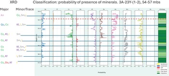
Core 3A: 3A-23Y-(1-2), 54–57 mbs
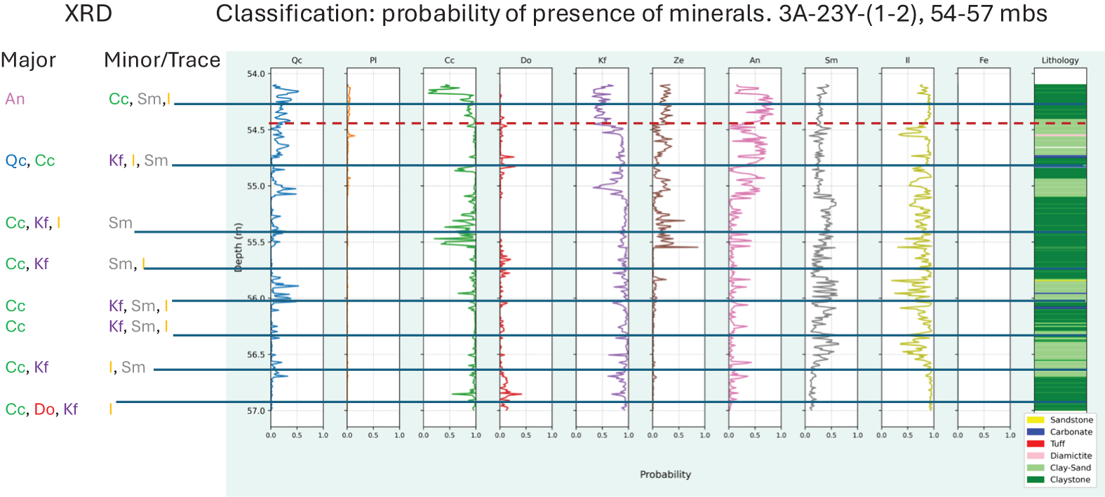
This interval represents lower Bed II in Core 3A. Core 3A records a deeper-water environment than Core 2A (particularly for Bed II) and is thus dominated by claystone, with only thin sandstone and a few layers with authigenic calcite crystal concentrations, some of which were interpreted by Hay and Kyser (Reference Hay and Kyser2001) as pseudomorphs after evaporite minerals but most of which were likely crystallized as calcite in equilibrium with lake water (Bennett et al., Reference Bennett, Marshall and Stanistreet2012). Calcite is present in all samples analyzed by XRD (McHenry et al., Reference McHenry, Kodikara, Stanistreet, Stollhofen, Njau, Schick and Toth2020a) for this interval, and K-feldspar (likely authigenic) in all but one. Both smectite and illite are identified in all samples; where one is more abundant, it is always illite. Only the uppermost sample contained a zeolite (analcime). Quartz is also only recognized in one sample (the second from the top).
The classification model for this interval (Fig. 5) predicts no quartz for almost all samples, with a few “spikes” barely exceeding 0.5. Calcite is predicted for almost every sample. While dolomite is not predicted in any sample at greater than 0.5 probability, it is notable that the most significant “spike” (0.415 at 56.854 mbs) corresponds approximately to the one XRD sample from this interval that identified dolomite (as a minor phase). Illite is predicted for almost all samples, whereas the probability of smectite exceeds 0.5 for some intervals between 55 and 56.5 mbs. No zeolites are predicted below 55.55 mbs, with only two (single sample) “spikes” for non-analcime zeolites above. Analcime is predicted to be absent below 55.2 mbs, but present in many samples above. This is consistent with the XRD observations, which had analcime as a common phase at 54.27 mbs (but not in samples below). The higher resolution provided by the core-scan XRF data–based model provides a more exact placement for this transition (to analcime bearing): it first appears at 55.054 mbs. The predicted presence of K-feldspar is also a good match for the XRD results—it is predicted (and observed) for all samples below 54.27 m, but it is less likely above (and not observed by XRD). This is a meaningful transition, as it also corresponds to the emergence of analcime. K-feldspar in this part of the core is likely an authigenic product, formed in the sediments at the expense of zeolites under highly saline-alkaline conditions (Hay and Kyser, Reference Hay and Kyser2001; McHenry, Reference McHenry2009, Reference McHenry2010, McHenry et al., Reference McHenry, Kodikara, Stanistreet, Stollhofen, Njau, Schick and Toth2020a). Extrapolating upward in the core, using the predictions of the classification model, analcime is predicted to be present in most samples up to at least 2A-16Y-1 (34.6 m), and in many intervals above that level, especially in claystone.
Classification model results for core interval 3A-23Y-(1-2), 54–57 m below surface (mbs), vs. lithological classes with X-ray diffraction (XRD) phase IDs for individual samples from McHenry et al. (Reference McHenry, Stanistreet, Stollhofen, Njau, Schick and Toth2020b). See Figure 3 caption for mineral abbreviations and for scale description. Plots show the likely presence of calcite and K-feldspar for most of this interval, with the probability of analcime increasing at the expense of K-feldspar above 54.5 mbs, indicated by the dashed red line. Illite is more likely than smectite for most of this interval.
The regression model (Fig. 6) supports the low abundance of quartz, with only two “spikes” (both tied to thin sandy intervals). Carbonates vary in predicted abundance, with high expected abundances in most intervals except for some claystone intervals with little carbonate. These low-carbonate intervals are instead enriched in zeolites and feldspar.
Regression model results for core interval 3A-23Y-(1-2), 54–57 m below surface (mbs), vs. lithological classes. See Figure 4 caption for mineral abbreviations and for scale description.

Olduvai Bed I to Bed II transition, Cores 2A and 3A
Core 2A-28Y-1 to 29Y-1, 64.9–67.4 mbs
This interval was selected because it includes the transition between Olduvai Beds I and II (Tuff IF), an important stratigraphic marker in outcrop and base of the “time slice” investigated in detail by the Olduvai Landscape Archaeology and Paleoanthropology Project (OLAPP; Blumenschine and Peters, Reference Blumenschine and Peters1998). It is well characterized in outcrop, where it is interpreted to coincide with a rapid lake recession and desiccation, recognized even near the lake depocenter (Stollhofen et al., Reference Stollhofen, Stanistreet, McHenry, Mollel, Blumenschine and Masao2008). XRD of the highly altered Tuff IF in Core 2A reveals mostly the zeolite mineral phillipsite and anorthoclase (residual from the primary tuff), with minor authigenic K-feldspar, smectite, and analcime. Directly beneath the tuff lies a dolomite layer, recognized in the core (and confirmed by XRD) and in outcrop at sites within the lake depocenter (e.g., Hay and Kyser, Reference Hay and Kyser2001).
The position of Tuff IF within the core is visible using the classification model (Fig. 7), based on the absence of carbonate and presence of non-analcime zeolites. Because anorthoclase is included in the “K-feldspar” group in the model, the predicted occurrence of K-feldspar in the Tuff IF interval is also consistent. Smectite is predicted for some samples within Tuff IF but is not as likely as it is for the enclosing claystone intervals. The dolomite layer below Tuff IF also shows up clearly, and its thickness is consistent with core descriptions. K-feldspar, identified as “minor” in most XRD samples, is predicted for most intervals. XRD samples with trace or no K-feldspar match up with intervals within the model with lower probabilities for K-feldspar. Quartz is predicted to be absent for most of the interval, although it is likely present in the lower part (in the more sandy claystone units). The one XRD sample from this interval that showed quartz in XRD is in this part of the core (at 67.12 mbs). Calcite is predicted throughout this section, except in Tuff IF, consistent with the XRD results. Smectite is predicted throughout most of the interval, consistent with XRD, with illite only predicted for one thin claystone above Tuff IF (unfortunately not represented in the XRD study). Overall excellent agreement is shown between the classification model, the XRD results, and the observed lithologies.
Classification model results for core interval 2A-28Y-1 to 29Y-1, 64.9-67.4 m below surface (mbs) vs. lithological classes with X-ray diffraction (XRD) phase IDs for individual samples from McHenry et al. (Reference McHenry, Stanistreet, Stollhofen, Njau, Schick and Toth2020b). See Figure 3 caption for mineral abbreviations and for scale description. This core interval includes marker Tuff IF (interval indicated by dashed red lines), identifiable here by its lower probability for containing calcite or dolomite and its higher probability of containing non-analcime zeolites, compared with enclosing claystone.
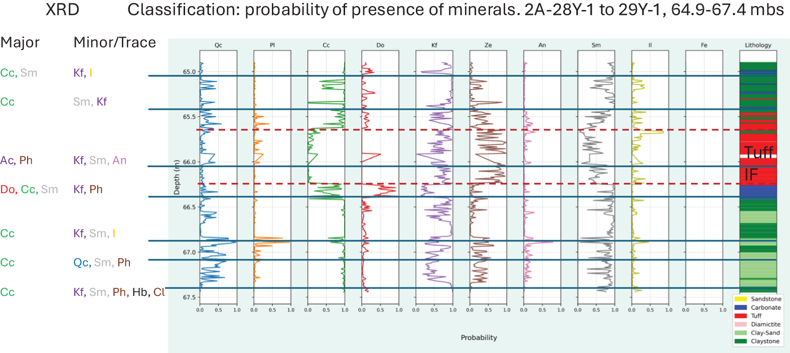
Of special interest in the classification model is the pattern of K-feldspar versus zeolite probabilities; where the model predicts the presence of K-feldspar, it does not predict zeolites, and vice versa. This is similar to the XRD-generated abundances for upper Bed I (McHenry et al., Reference McHenry, Kodikara, Stanistreet, Stollhofen, Njau, Schick and Toth2020a, Reference McHenry, Gebregiorgis and Foerster2023), where this pattern was interpreted to indicate the formation of authigenic K-feldspar at the expense of zeolites at times of increased saline-alkaline conditions in the paleolake basin.
The regression model also clearly predicts the position of Tuff IF, with abundant zeolite, generally high feldspars, negligible carbonate, and lower amounts of clay minerals within this unit compared with units above and below (Fig. 8). Because carbonates are combined in the regression model, the dolomite layer does not stand out as well in this data. Carbonates are predicted to be the most abundant components of samples from the bottom of this interval (below 66.25 mbs), consistent with XRD results showing abundant calcite and only minor amounts of other phases. The core descriptions document calcite crystal-rich layers in this section.
Regression model results for core interval 2A-28Y-1 to 29Y-1, 64.9–67.4 m below surface (mbs) vs. lithological classes. See Figure 4 caption for mineral abbreviations and for scale description. Tuff IF is identifiable in the model results by its lower abundance of carbonate, increased abundance of zeolite, and lower abundance of clay compared with enclosing claystone.

Core 3A-24Y-(1- 2), 57–60 mbs
This section was selected because it also includes Tuff IF, the uppermost. unit of Olduvai Bed I. As this transition was also considered for Core 2A, it provides the opportunity to compare the two cores. Only five XRD analyses cover this range (McHenry et al., Reference McHenry, Kodikara, Stanistreet, Stollhofen, Njau, Schick and Toth2020a), and none included any data for the tuffs or for the carbonate layer underlying Tuff IF (which was dominated by dolomite in Core 2A). General trends based on XRD show calcite and K-feldspar throughout, with illite in the basal two samples and more smectite above. Zeolites (phillipsite or analcime) are only minor or trace phases (in the claystone and sandstone sampled), if present at all.
The classification model provides more detail (Fig. 9). First, it clearly predicts the position of Tuff IF (consistent with core lithology), based on an abrupt absence of calcite and dolomite and an abrupt increase in the probability of non-analcime zeolites. The probability of dolomite is highest directly beneath Tuff IF, at the position of the marl from the core description. K-feldspar and zeolites are also not predicted for this dolomite layer. Calcite is predicted to be present throughout, except in Tuff IF and a few individual data points below. The XRD data point at 59.57 mbs is difficult to reconcile with the classification model. Based on XRD, this should contain dolomite, analcime, and illite (with no calcite and only trace K-feldspar), but the model does not predict any dolomite and puts calcite at a high probability for this point and for neighboring points. Analcime is possible (greater than 0.5 probability at 59.578 mbs) and illite is also likely.
Classification model results for core interval 3A-24Y-(1-2), 57–60 m below surface (mbs), vs. lithological classes with X-ray diffraction (XRD) phase IDs for individual samples from McHenry et al. (Reference McHenry, Stanistreet, Stollhofen, Njau, Schick and Toth2020b). See Figure 3 caption for mineral abbreviations and for scale description. This Core 3A interval also includes marker Tuff IF, which shows up clearly with its lower probabilities for calcite, dolomite, and analcime, combined with its higher probabilities for non-analcime zeolites.

As in the equivalent interval in Core 2A, aside from the tuffs and dolomite layer, the probabilities for K-feldspar and zeolites follow opposite patterns (where one is higher, the other is low), although the overall likelihood of non-analcime zeolites outside Tuff IF is lower in Core 3A.
The regression model for this part of Core 3A (Fig. 10) also shows the position of Tuff IF (little carbonate, abundant zeolites and K-feldspar). Because the regression model does not differentiate dolomite from calcite, the dolomite layer beneath Tuff IF cannot be isolated from the overall high carbonate abundances below Tuff IF. In general, the sediments beneath Tuff IF are predicted to be dominated by carbonate and clay minerals, consistent with the XRD results. Other phases are only present at the trace or minor level.
Regression model results for core interval 3A-24Y-(1-2), 57–60 m below surface (mbs), vs. lithological classes. See Figure 4 caption for mineral abbreviations and for scale description. Tuff IF is identifiable based on its higher predicted abundance of zeolites and feldspar and lower abundance of carbonate compared with surrounding sediments. Other thinner tuff beds in the same interval do not provide as strong a signal.

Olduvai Bed I (Core 3A)
3A-31Y-2, 79.5–81 mbs
This interval represents the top of a thick marl unit best observed in Core 3A, which represents a deeper-water facies assemblage than present in Core 2A. It contains a thin altered tuff toward the top but otherwise consists of carbonate-rich claystone and marl. Dolomite, calcite, and aragonite are all identified by XRD, although calcite is only recognized as a minor phase. Smectite is also abundant in all samples.
The classification model (Fig. 11) is consistent with the XRD observations. Dolomite is likely throughout this part of the core, except for at the very top (above the tuff). Calcite is predicted for the claystone part of the section but less likely in the marl (below 80.5 mbs), its probability drops to below 0.5 right at the transition noted in the core lithological description. Because aragonite and calcite are polymorphs, the model does not distinguish between them. Smectite is predicted to be present throughout, with no illite. The top of the core is predicted to contain non-analcime zeolites. Although not recognized in XRD, this does make sense lithologically, given the identified tuff (for which no XRD data are available). The XRD results from the section immediately above the selected interval do register zeolites, notably phillipsite.
Classification model results for core interval 3A-31Y-2, 79.5–81 m below surface (mbs), vs. lithological classes with X-ray diffraction (XRD) phase IDs for individual samples from McHenry et al. (Reference McHenry, Stanistreet, Stollhofen, Njau, Schick and Toth2020b). See Figure 3 caption for mineral abbreviations and for scale description. This interval contains the top of a dolomitic marl, which can be seen in the high probability of dolomite. Increased zeolite probabilities toward the top correspond to a thin tuff bed (dashed red line).

The regression model (Fig. 12) predicts high carbonate abundances throughout, with slightly lower abundances toward the top of the interval where zeolite is slightly more abundant. The sharp peak in predicted zeolite abundance (and drop in carbonate) at 79.7 mbs corresponds with the thin tuff there.
Regression model results for core interval 3A-31Y-2, 79.5–81 m below surface (mbs), vs. lithological classes. See Figure 4 caption for mineral abbreviations and for scale description.

3A-39Y-(1-2), 99.2–102 mbs
This core interval was selected because it represents a time period within Lower Olduvai Bed I that is found exclusively in Core 3A (and is absent due to an unconformity in both Cores 1A and 2A). The XRD results showed it to be free of zeolites and authigenic K-feldspar, indicating likely fresher conditions than the rest of Bed I above. The specific interval also covers a transition from calcite-free to calcite-rich, and from illite to smectite as the dominant clay. Minor to trace feldspar (anorthoclase or plagioclase) is observed in all XRD samples in this interval.
The classification model (Fig. 13) shows a transition at about 100.2 mbs for multiple minerals. Illite transitions to smectite, the probability of quartz drops from around 0.5 to near zero, and the probability of K-feldspar and non-analcime zeolites increases. The probability of calcite abruptly increases from near zero to almost certain at around 99.7 mbs. The probability for dolomite also increases, although it is less uniform between samples compared with calcite. The probability of iron-bearing minerals is also enhanced in the upper part of the core. Although no iron-bearing minerals were observed in the XRD results for samples in this interval, the sample immediately overlying this interval (at 98.9 mbs) contains minor pyrite and the detailed core descriptions identified two pyrite-bearing horizons at the appropriate positions (99.35 and 99.57 mbs). Some of these trends are readily apparent in the XRD data—for example, the illite to smectite transition and emergence of calcite. However, the increase in probability for non-analcime zeolites is not evident in the XRD data. The XRD samples at 99.86 and 100.16 mbs should fall within the zeolite-bearing zone according to the model but did not register any zeolite. The only quartz registered by XRD occurs in the lower part of the interval, where the classification model predicts its presence.
Classification model results for core interval 3A-39Y-(1-2), 99–102 m below surface (mbs), vs. lithological classes with X-ray diffraction (XRD) phase IDs for individual samples from McHenry et al. (Reference McHenry, Stanistreet, Stollhofen, Njau, Schick and Toth2020b). See Figure 3 caption for mineral abbreviations and for scale description. The increased probability of iron-bearing phases in the upper part of this interval corresponds with pyrite in the core descriptions (indicated on the lithology column by orange diamonds). The transition from illite to smectite, and the abrupt increase in carbonate, are consistent with XRD results, however the increase in zeolite abundance is not; no zeolites were identified by XRD in this part of the core.

The regression model (Fig. 14) predicts abundant zeolite in the upper part of this core interval (for the same interval predicted in the classification model), but again the XRD results do not support this. We even re-ran the two collected samples from this interval using XRD (with a newer XRD instrument with lower backgrounds) to double-check and found no zeolite. The lower estimated abundances of clay minerals in the same interval also do not appear to be supported by the XRD data. An inspection of the core image for the modeled zeolite-rich section reveals a bioturbated but notably darker and largely featureless claystone unit compared with the units above and below. In the regression model, the increased abundance of zeolite correlates to a decreased abundance of clay minerals. As neither trend was observed in XRD, it is likely that this trend could be explained by a change in clay composition for which the model was not trained
Regression model results for core interval 3A-39Y-(1-2), 99–102 m below surface (mbs), vs. lithological classes. See Figure 4 caption for mineral abbreviations and for scale description. The transition to carbonate-rich sediment is consistent with X-ray diffraction (XRD) results, but the peak in zeolite intensity is not.

Ngorongoro Formation (volcanic), Core 2A
Core 2A-51Y-2, 130.45–131.9 mbs
This interval was chosen to represent the tuffs of the Ngorongoro Volcanic Formation. Only two samples from this interval were run by XRD (McHenry et al., Reference McHenry, Kodikara, Stanistreet, Stollhofen, Njau, Schick and Toth2020a). These tuffs and pyroclastic flow deposits still contain volcanic glass (registered in XRD as an amorphous “hump”) along with abundant anorthoclase feldspar and the non-analcime zeolites erionite (major) and chabazite (minor). The tephra composition of these units (from McHenry et al., Reference McHenry, Stanistreet, Stollhofen, Njau, Schick and Toth2020b), based on electron microprobe analysis of phenocrysts and glass, reveal a rhyolitic composition, with altered glass and primary phenocryst phases dominated by anorthoclase feldspar and augite with minor titanomagnetite and ilmenite—no quartz was recorded.
The classification model for this interval (Fig. 15) predicts quartz, plagioclase, and non-analcime zeolites throughout, with no clay or carbonate minerals. K-feldspar probability exceeds 0.5 for much of this interval, and analcime exceeds it occasionally. The positions of the two XRD control points happen to fall at positions where quartz, plagioclase, and analcime are notably low, which is consistent with the XRD results showing only anorthoclase (categorized as K-feldspar) and non-analcime zeolites. The regression model (Fig. 16) predicts high abundances for feldspars and zeolites, variable abundance for quartz, and little to no clay minerals. Carbonates are predicted at moderate abundances only for a few samples (and are otherwise absent).
Classification model results for core interval 2A-51Y-2, 130.45–131.9 m below surface (mbs), vs. lithological classes with X-ray diffraction (XRD) phase IDs for individual samples from McHenry et al. (Reference McHenry, Stanistreet, Stollhofen, Njau, Schick and Toth2020b). See Figure 3 caption for mineral abbreviations and for scale description. This core interval is entirely composed of less altered tuff from the Ngorongoro Formation. Clay and carbonate probabilities are low, whereas feldspar, quartz, and zeolite probabilities are high. XRD did not reveal zeolite for this interval, instead showing volcanic glass (a phase not considered in this model).

Regression model results for core interval 2A-51Y-2, 130.45–131.9 m below surface (mbs), vs. lithological classes. See Figure 4 caption for mineral abbreviations and for scale description.

One major limitation of the model in this part of the core is that volcanic glass was not considered when building the model, and even if it was, the trachytic compositions of Bed I and the rhyolitic compositions of the Ngorongoro Formation may complicate the modeling. The contribution of the glass to the overall composition is thus divided between phases included in the model, including quartz, plagioclase, and zeolites. This model predicts that rhyolitic glass-bearing intervals are richer in quartz than they actually are (because high silica from the glass is almost certainly being attributed to quartz), and it predicts a high probability of plagioclase in a rhyolite that contains none (but which does have abundant anorthoclase, classified with the K-feldspar). This highlights the importance of using the phases abundant in the cores to build and train the models and applying the models only to cores with relevant mineral assemblages.
Naibor Soit Formation, Core 2A
Core 2A-65Y-(1-2), 168–170.9 mbs
This interval was chosen to represent the upper Naibor Soit Formation, newly discovered in core and unknown from outcrop. This fluviolacustrine interval lies between the two major volcanic pulses of the Ngorongoro Formation and is mineralogically distinct from the well-studied Olduvai Beds Formations above. The specific interval selected contains no coarse units, only claystone and sandy claystone. Based on XRD (McHenry et a. 2020a), quartz should be abundant in the top of the interval and at the very base (in clayey sandstone) but absent in the middle. Non-analcime zeolites (chabazite and erionite) were identified in all XRD samples, although sometimes as only minor phases. Feldspar is identified in most samples but tends to be either anorthoclase or plagioclase (rather than K-feldspar). Illite is present in all samples, whereas calcite is present in a few samples.
The classification model is much noisier for this interval than for those described from the Olduvai Formation (Fig. 17). Quartz, plagioclase, calcite, and analcime swing wildly from definitively present to absent. Quartz and plagioclase are predicted to be present throughout the upper part of this interval (above 168.8 mbs), which is consistent with the XRD results. Both are also expected to be present at the base of the interval (below 170.65 mbs), which is consistent with XRD for quartz but not for plagioclase (anorthoclase is abundant for this interval according to XRD, but has been lumped with K-feldspar in the model). A point-by-point comparison of the classification model results against XRD for calcite reveals that the five samples for which calcite was identified by XRD correspond to samples modeled to have high probabilities of calcite, while most that did not contain calcite in their diffraction patterns had lower probabilities in the model. The prediction of analcime is particularly problematic, as it was not identified in a single sample by XRD. A point-by-point comparison of the model data to the equivalent XRD data shows that in most cases, the XRD samples correspond to intervals with lower probability for analcime. But the bottom two samples (at 170.6 and 170.9 mbs) are in the middle of intervals with higher probabilities that did not yield analcime in their XRD patterns. Also problematic is that non-analcime zeolites have moderate to low probabilities in the lowest meter of this interval, yet are identified in all XRD samples, in some cases as common constituents. Illite is accurately predicted as the dominant clay.
Classification model results for core interval 2A-65Y-(1-2), 168–170.9 m below surface (mbs), vs. lithological classes with X-ray diffraction (XRD) phase IDs for individual samples from McHenry et al. (Reference McHenry, Stanistreet, Stollhofen, Njau, Schick and Toth2020b). See Figure 3 caption for mineral abbreviations and for scale description. This core interval represents the Naibor Soit Formation. The high level of “noise” in the probabilities for quartz, plagioclase, calcite, and zeolites likely reflects actual mineralogical variability over short time intervals, as this sample-to-sample variability is also observed in the XRD data, but it could also be attributed to lack of adequate model training. The model predicts the presence of analcime throughout much of this core section, but it was not detected in any of the XRD samples (which all happen to coincide with dips in its probability). Conversely, non-analcime zeolites are detected in all XRD samples, although the probability of their presence is on average lower than that of analcime.

The regression model for this interval (Fig. 18) is also noisy, with many abrupt transitions in mineral abundance. Where present, carbonates and feldspars are predicted to have the greatest abundances. The combined zeolite category has a steadier, more moderate abundance. Quartz is more abundant near the base and top of this section, consistent with its higher probabilities in the classification model. The apparent “noise” in this part of core likely represents real variations in the presence and abundance of specific phases, which also vary sample-to-sample in the XRD results.
Regression model results for core interval 2A-65Y-(1-2), 168–170.9 m below surface (mbs), vs. lithological classes. See Figure 4 caption for mineral abbreviations and for scale description.

Overall trends for the models versus XRD mineralogy and core descriptions
The models described in Kodikara et al. (Reference Kodikara, McHenry, Stanistreet, Stollhofen, Njau, Toth and Schick2024) were developed using intensity ratios from the core-scan XRF data, XRD-derived mineral identifications, and lithology (from the core sedimentological descriptions), but did not consider stratigraphic position. Within those constraints, the optimized DNN classification model achieved greater than 86% binary accuracy with unseen data in terms of being able to accurately predict the minerals present (at above the trace level). The current study applies these models to all XRF data points (within the modeled lithologies) and also ties them to their stratigraphic position, making it possible to use more lithological information to interpret the quality of the fit.
The core sections described in the previous sections represent typical intervals for the finer-grained fluviolacustrine portions of Cores 2A and 3A, with one section representing the Ngorongoro Volcanic Formation (tuffs and pyroclastic flows). Within these sections, the model predictions appear to be well suited for:
1. identifying dolomite-rich layers;
2. distinguishing between carbonate-rich and carbonate-poor intervals;
3. identifying intervals of sandstone within claystone-dominated sediments;
4. identifying (altered) tuffs within claystone-dominated sediments; and
5. predicting which clay (illite or smectite) is dominant.
The models also struggled in some areas:
1. less-altered tuffs of the Ngorongoro Formation (rhyolitic glass, not considered in the model, is interpreted as quartz and zeolite); and
2. analcime and non-analcime zeolites in non-tuff sediments, especially where the non-analcime zeolite is not phillipsite.
Increased probabilities for zeolites (and increased predicted abundances) help to clearly identify tuff layers, but their presence and abundances in other sediment types is more problematic. This can result either in the prediction of zeolites in sections of the cores in which none are detected by XRD (e.g., Core 3A lower Bed I: 3A-39Y-(1-2) [99.2-102 mbs] [Figures 13-14]) or the failure to predict zeolites in sections of the cores for which they are identified in XRD as common constituents (e.g., Core 2A Naibor Soit Formation: 2A-65Y-(1-2) [168–170.9 mbs] [Figures 17-18). Notably, the zeolite predictions appear to be a better fit for the XRD data in the upper part of the cores (Bed II and upper Bed I) and worse in lower Bed I and the Naibor Soit Formation. This could be related to the specific zeolites; the upper Beds are dominated by phillipsite and analcime, whereas in the Ngorongoro and Naibor Soit Formations, chabazite and erionite are the dominant non-analcime zeolites. The “non-analcime zeolite” category includes phillipsite, chabazite, erionite, and clinoptilolite, but the model appears to work best for units where phillipsite dominates (e.g., Bed II and upper Bed I).
One fundamental consideration for any model that predicts mineral assemblages based on elemental composition is that different mineral assemblages can add up to the same bulk composition. This is especially true in closed-basin environments, where dissolved components are more likely to be re-precipitated or re-incorporated locally, rather than leached and removed from the system. McHenry (Reference McHenry2009, Reference McHenry2010) investigated the bulk elemental compositions, mineral assemblages, and mineral compositions of Olduvai Tuff IF altered in different environments across the Olduvai basin, and found that while bulk composition changed very little, alteration assemblages varied considerably, with the same bulk composition achieved through different abundances of clay versus zeolite minerals and different clay and zeolite elemental compositions. This can be seen in the current study, where the bulk compositions of less-altered tuffs of the Ngorongoro Formation, composed largely of volcanic glass, yield quartz, feldspar, and zeolite assemblages in the models. Zeolites and feldspars have similar elemental compositions (and many zeolites overlap each other in composition as well).
The closed-basin saline-alkaline lake environment allows for considerable differences in authigenic mineral assemblages (different zeolites, clays, and carbonates) associated with only minor changes in bulk elemental composition, complicating our ability to extract mineralogical interpretations from core-scan XRF elemental data. The models do better when there is a difference in the source of the sediments—for example, quartz-rich fluvial input from the western to southwestern metamorphics versus weathered volcanics from the Ngorongoro Volcanic Highlands to the east and south versus fine-grained authigenic lacustrine sediments. Mineralogical differences tied to in situ alteration or authigenesis (resulting from changes in lake conditions or fluid composition) are more difficult to identify based on bulk elemental composition alone.
Mineral assemblages in saline and alkaline lacustrine environments typically exhibit varying degrees of disequilibrium, as the precipitation and preservation of individual mineral phases are strongly influenced by kinetic constraints associated with fluctuations in temperature, salinity, and brine chemistry, as well as episodic changes in hydrological and redox conditions (Chase et al., Reference Chase, Arizaleta and Tutolo2021). High-resolution XRF and micro-XRF scanning techniques are most effective in sedimentary successions in which mineral assemblages are closer to equilibrium—such as well-lithified Paleozoic sandstones and shales—where chemical signatures tend to be compositionally homogeneous and diagenetically stable (Gabriel et al., Reference Gabriel, Reinhardt, Chang and Bhattacharya2022). Therefore, it is important to further evaluate the performance of the DNN-based approach on such equilibrium-prone core materials to assess its general applicability and robustness across diverse sedimentary contexts.
Considerations for model improvement
The model developed was limited by the training dataset. To differentiate volcanic glass from quartz, the model would require enough training data representing glass. Unfortunately, the training set only had 19 data points (out of 425 total) containing glass, which is insufficient for model development, even if we use the other associated minerals or lithologies for the deep learning models. Additional XRD analysis of fresher tuffaceous units of the Ngorongoro Formation (where glass is present) could help address this specific shortcoming, but in general, minerals and mineral groups that occur less frequently in the cores are more difficult to incorporate into the models.
It is extremely difficult to identify different zeolite minerals using their elemental ratios alone, even with a full geochemical analysis. A reliable classification is only possible based on mineral structure considerations (Passaglia and Sheppard, Reference Passaglia, Sheppard, Bish and Ming2002). If distinguishing individual zeolites from one another is important for a study, a separate model focusing on zeolites could potentially be developed, introducing new element ratios based on previous zeolite research, such as complex elemental intensity ratios like Si/(Al+Fe), modified after Hay and Sheppard (Reference Hay, Sheppard, Bish and Ming2001), and (Ca + Mg)/(Na + K) after Langella et al. (Reference Langella, Cappelletti, Gennaro, Bish and Ming2001). In the trained model, Kodikara et al. (Reference Kodikara, McHenry, Stanistreet, Stollhofen, Njau, Toth and Schick2024) used only the major elements, including Al, Ca, Fe, K, Mg, S, and Si, yet some minor elements are also available in the core-scan XRF database. Some minor elements, such as Ba and Sr, may sometimes be present as fundamental, subordinate, or occasional elements in zeolites (Passaglia and Sheppard, Reference Passaglia, Sheppard, Bish and Ming2002), and their inclusion in the models could yield new associations.
The high probability of co-occurrence of tuff with analcime in the training data gives more weight to the high probability of predicting analcime when high Si and Na are present in units identified as tuff. This needs to be carefully addressed in future models, by obtaining more XRD data from samples where analcime is absent in tuff layers (e.g., less-altered or erionite- and chabazite-dominated altered tuffs of the Ngorongoro Formation, which are underrepresented in the XRD dataset) or present in non-tuff layers.
Kodikara et al. (Reference Kodikara, McHenry, Stanistreet, Stollhofen, Njau, Toth and Schick2024) used the mineral abundance data documented by McHenry et al. (Reference McHenry, Kodikara, Stanistreet, Stollhofen, Njau, Schick and Toth2020a), which are reported as qualitative abundance based on relative XRD peak heights. They categorized the relative mineral abundances into four classes: “Abundant,” “Common,” “Minor,” and “Trace.” However, Kodikara et al. (Reference Kodikara, McHenry, Stanistreet, Stollhofen, Njau, Toth and Schick2024) only used “Abundant,” “Common,” and “Minor” as 3, 2, and 1, respectively, and later rescaled them to a 0–1 scale, assuming that “Trace” minerals may not be reflected in elemental data and intending to reduce the complexity. This cascaded shift from qualitative to quantitative followed by rescaling will also affect the predictive results. XRD analysis of future OGCP cores will be more quantitative, introducing the use of an internal standard to help better calibrate peak heights to actual mineral abundances and better account for non-diffracting phases.
Kodikara et al. (Reference Kodikara, McHenry, Stanistreet, Stollhofen, Njau, Toth and Schick2024) used simplified, combined lithological classes for the training data (e.g., tuff and volcanoclastic sandstone as tuff; calcite, dolomite, and marl as carbonate). This reliance on existing lithological descriptions limits the applicability of these models to new cores for which data are not yet available. A future iteration of this model could make use of the tone, color, and texture of associated RGB images (derived using a convolutional neural network) instead of lithological classes to train the dataset. In this way, we would be able to fully automate the mineral identification process using only the XRF scan and RGB image data, providing predictions that could then aid in sedimentological analysis and sample prioritization.
Rapid paleoenvironmental fluctuations detected by the model
The results of this model application provide predictions about the presence and absence of authigenic minerals throughout the fluviolacustrine intervals of the Olduvai Beds, which can be used to locate major lithological transitions and identify higher-frequency changes in the depositional environment. Stanistreet et al. (Reference Stanistreet, Boyle, Stollhofen, Deocampo, Deino, McHenry, Toth, Schick and Njau2020a) used the same core-scan XRF data as an elemental proxy for changes in paleoenvironment for Olduvai Bed I and part of Bed II, and found that the ratio of Mg to Al (and the XRF counts for Ti) yielded a likely high-resolution climate signal. They interpreted higher Al and Ti as indicators of added detrital input, due to higher-energy input to the Olduvai basin (during wetter intervals) and the contribution of detrital pedogenic clays washed into the basin. Elevated Mg was instead tied to lower-energy authigenic formation of Mg clays, during times of less detrital input. They found that these elements and element ratios showed cyclicity that could be matched to other paleoenvironmental indicators, including hydrogen isotopes (Colcord et al., Reference Colcord, Shilling, Freeman, Njau, Stanistreet, Stollhofen, Schick, Toth and Brassell2019). However, the Stanistreet et al. (Reference Stanistreet, Boyle, Stollhofen, Deocampo, Deino, McHenry, Toth, Schick and Njau2020a) paper did not establish the changes in mineralogy associated with these element and element ratio changes.
McHenry et al. (Reference McHenry, Kodikara, Stanistreet, Stollhofen, Njau, Schick and Toth2020a) used the XRD-derived mineral assemblages as proxies for changes in lake conditions, although at a 32 cm sampling interval, these data lack the high-resolution coverage of the core-scan XRF data. The current study helps extrapolate between the two resolutions, using the XRD results to test model predictions for higher-resolution changes in mineral assemblage. The core interval immediately surrounding Tuff IF at the transition from Olduvai Bed I to Bed II, shown in Figure 7 for Core 2A (2A-28Y-1 to 29Y-1, 64.9–67.4 mbs) and in Figure 9 for Core 3A (3A-24Y-(1-2), 57–60 mbs), is a good example. Stanistreet et al. (Reference Stanistreet, Boyle, Stollhofen, Deocampo, Deino, McHenry, Toth, Schick and Njau2020a) recognized cycles in the Mg/Al and Ti core-scan XRF data for this interval, with elevated Mg/Al indicating drier intervals and elevated Ti indicating wetter conditions. McHenry et al. (Reference McHenry, Kodikara, Stanistreet, Stollhofen, Njau, Schick and Toth2020a) found that in this interval, the driest intervals corresponded to elevated authigenic K-feldspar, while intermediate intervals had less K-feldspar and more zeolite, typically phillipsite. The wettest conditions had neither K-feldspar nor zeolite. The results of the current model identify the same trend, with alternating intervals with high probabilities for K-feldspar or zeolite (Fig. 7). The model predicts even shorter intervals of alternating K-feldspar and zeolite than McHenry et al. (Reference McHenry, Kodikara, Stanistreet, Stollhofen, Njau, Schick and Toth2020a), as some transitions occur within a single 32 cm XRD sampling interval.
The application of this model to OGCP Cores 2A and 3A shows frequent transitions between drier (authigenic K-feldspar) and wetter (zeolite) intervals, some of which were captured in the XRD study (McHenry et al., Reference McHenry, Kodikara, Stanistreet, Stollhofen, Njau, Schick and Toth2020a), and some of which were not due to insufficient sampling resolution. These also correspond well with the elemental cyclicity described in Stanistreet et al. (Reference Stanistreet, Boyle, Stollhofen, Deocampo, Deino, McHenry, Toth, Schick and Njau2020a), which they linked to insolation and more regional or global climate events.
Conclusions
Application of the wide and deep learning models developed in Kodikara et al. (Reference Kodikara, McHenry, Stanistreet, Stollhofen, Njau, Toth and Schick2024), based on core-scan XRF and lithological descriptions of the OGCP 2014 cores from the Olduvai basin, Tanzania, to identify mineral assemblages, met with mixed success. Compared with XRD data from the same cores, the models were excellent at predicting the positions of dolomite layers, carbonate-rich intervals, tuffs within claystone, and smectitic versus illitic clay-rich intervals. The models struggled to correctly identify zeolite-rich intervals, especially those not associated with tuffs or where the zeolite minerals were chabazite and/or erionite (rather than phillipsite or analcime), or for less-altered tuffs such as those in the Ngorongoro Formation, where glass rather than zeolite prevails. Given that paleolake Olduvai was a closed basin and that much zeolitization occurs through in situ alteration, it is not surprising that element ratios alone are insufficient to reconstruct some mineral assemblages. Therefore, expanding the dataset with quantitative XRD data and diverse lithologies, along with integrating complex element ratios and RGB image features, would significantly enhance the accuracy, automation, and overall robustness of XRF-based deep learning models for mineral and sedimentological analysis.
Supplementary material
The supplementary material for this article can be found at https://doi.org/10.1017/qua.2025.10060
Acknowledgments
We would like to thank the Stone Age Institute, which organized and funded the Olduvai Gorge Coring Project (OGCP) and subsequent XRF scanning of the core with support from the Kaman Foundation, the Gordon and Ann Getty Foundation, the John Templeton Foundation, the Fred Maytag Foundation, and Kay and Frank Woods. We also thank the Commission for Science and Technology (COSTECH), the Department of Antiquities, the Ministry of Natural Resources and Tourism (MNRT), and the Ngorongoro Conservation Area Authority (NCAA) in Tanzania for granting permission to conduct research in Tanzania. We thank Anders Noren, Kristina Brady, and the staff of the LacCore facility (now the Continental Scientific Drilling Facility) at the University of Minnesota, Twin Cities, for all their support with sampling the core. We also thank Erik Brown and Wally Lingwall of the Large Lakes Observatory, University of Minnesota, Duluth, who undertook the XRF scanning of the core. Many thanks to the C, Python, Keras, NumPy, Matplotlib, R, and R package diagram developers.
Financial support
XRD analyses were additionally supported by the National Science Foundation (BCS grant no. 1623884 to JKN and LJM). Computational work was also supported by NASA SSW grant NNH20ZDA001N.
Competing interests
The authors declare that they have no financial interest directly or indirectly related to the work submitted for publication.


 Open access