





1. Introduction
Low-order models are an enabling tool in fluid dynamics, providing unique opportunities for rapid prediction and forecasting, estimation and control, and design optimisation (Benner, Gugercin & Willcox Reference Benner, Gugercin and Willcox2015; Brunton & Noack Reference Brunton and Noack2015; Rowley & Dawson Reference Rowley and Dawson2017). However, most use-cases require that low-order models remain faithful to the physics and underlying dynamics of the flows under consideration. This can be especially challenging in aerodynamics applications because the difficulty of crafting a low-order model that faithfully captures the essential physical and dynamical processes of a flow grows with increasing Reynolds number (Moehlis, Faisst & Eckhardt Reference Moehlis, Faisst and Eckhardt2004; Cavalieri & Nogueira Reference Cavalieri and Nogueira2022).
In fluid dynamics, low-order models have traditionally been obtained within the framework of projection-based model reduction (Holmes et al. Reference Holmes, Lumley, Berkooz and Rowley2012), whereby the Navier–Stokes equations are projected onto a low-dimensional subspace (e.g. Galerkin projection onto a subspace spanned by dominant proper orthogonal decomposition (POD) modes). Indeed, projection-based reduced-order models (ROMs) have proven a powerful tool for distilling the complex dynamics of unsteady flows into a compact set of ordinary differential equations (ODEs) that support real-time analysis, optimisation and predictive control (Rowley & Dawson Reference Rowley and Dawson2017; Taira et al. Reference Taira, Brunton, Dawson, Rowley, Colonius, McKeon, Schmidt, Gordeyev, Theofilis and Ukeiley2017; Brunton, Noack & Koumoutsakos Reference Brunton, Noack and Koumoutsakos2020; Taira et al. Reference Taira, Hemati, Brunton, Sun, Duraisamy, Bagheri, Dawson and Yeh2020).
Despite demonstrated successes in obtaining simplified yet physically faithful models in fluid dynamics, projection-based model reduction can be difficult to implement in practice. Projection-based approaches often demand full access to the governing equations and their discretisations – an intrusive requirement that limits their applicability, especially when working with complex computational fluid dynamics (CFD) codes (Peherstorfer & Willcox Reference Peherstorfer and Willcox2016). Projection-based model reduction can also result in models that diverge due to neglected energy transfers (Cazemier, Verstappen & Veldman Reference Cazemier, Verstappen and Veldman1998; Schlegel & Noack Reference Schlegel and Noack2015).
In contrast, data-driven frameworks – such as sparse identification of nonlinear dynamics (SINDy) (Brunton et al. Reference Brunton, Proctor, Kutz and Bialek2016; Loiseau & Brunton Reference Loiseau and Brunton2018), physics-informed neural networks (Raissi, Perdikaris & Karniadakis Reference Raissi, Perdikaris and Karniadakis2019; Thuerey et al. Reference Thuerey, Weißenow, Prantl and Hu2020), operator learning (Lu et al. Reference Lu, Jin, Pang, Zhang and Karniadakis2021) and operator inference (Peherstorfer & Willcox Reference Peherstorfer and Willcox2016; Kramer, Peherstorfer & Willcox Reference Kramer, Peherstorfer and Willcox2024) – are non-intrusive, inferring compact dynamical systems directly from data generated by CFD or measured in experiments. The data-driven approach enables rapid model construction and deployment even when a first-principles description is unavailable or only partially observed (Brunton et al. Reference Brunton, Proctor, Kutz and Bialek2016; Raissi et al. Reference Raissi, Perdikaris and Karniadakis2019).
Nonetheless, low-order models obtained from data-driven frameworks have their own limitations as well, often failing to generalise outside training datasets and commonly yielding unphysical energy growth under extrapolation (Duraisamy, Iaccarino & Xiao Reference Duraisamy, Iaccarino and Xiao2019; Karniadakis et al. Reference Karniadakis, Kevrekidis, Lu, Perdikaris, Wang and Yang2021). As such, much work has focused on ensuring that data-driven models adhere to known physical laws (e.g. conservation of mass, momentum and energy). In the case of incompressible flows, the quadratic nature of the convective nonlinearity in the Navier–Stokes equations admits energy transfer between modal triads – so-called triadic interactions (Schmidt Reference Schmidt2020). Furthermore, the divergence-free condition on the velocity field along with mild assumptions regarding boundary conditions results in the convective nonlinearity being lossless – i.e. the quadratic terms are energy preserving, only serving to redistribute kinetic energy without net production or dissipation. Data-driven methods have been developed to impose these physics-based constraints within modelling frameworks (Loiseau & Brunton Reference Loiseau and Brunton2018); however, the enforcement of lossless quadratic terms is not sufficient to guarantee that resulting models will maintain physically viable predictions over long-time horizons. Indeed, it is common for such models to yield predictions that grow unbounded with time – an indicator of unphysical behaviour. This is particularly problematic in flow control and estimation applications: a ROM that is not globally bounded may diverge or exit its regime of validity, undermining any controller or estimator based on it.
Notions of stability and boundedness have been investigated and developed to contend with the possibility of this unphysical feature in the dynamics of low-order models. Methods have been proposed for efficiently analysing the asymptotic stability of quadratic ROMs (Kramer Reference Kramer2021; Enayati Kafshgarkolaei & Hemati Reference Enayati Kafshgarkolaei and Hemati2025) or for directly identifying asymptotically stable ROMs from data (Goyal, Duff & Benner Reference Goyal, Duff and Benner2024). However, asymptotic stability is often a stronger condition than would be desired in many aerodynamics applications where trajectories remain bounded with time, but do not necessarily asymptote to an equilibrium point (e.g. wake shedding from an aerofoil). For such systems, it is natural to consider notions of long-time boundedness of trajectories (Khalil Reference Khalil2002).
Prior work by Schlegel & Noack (Reference Schlegel and Noack2015) studied the problem of long-time boundedness and established that quadratic dynamical systems whose quadratic nonlinearity is lossless can admit a trapping region – a monotonically attracting invariant set within which all trajectories remain indefinitely. The Schlegel and Noack trapping theorem provides conditions for the existence of a trapping region, which can be used to prove the long-time boundedness of projection-based ROMs for incompressible flows via non-convex optimisation (Schlegel & Noack Reference Schlegel and Noack2015). The theorem also provides a (conservative) upper bound on the size of the trapping region, if one exists. Recent work by Kaptanoglu et al. (Reference Kaptanoglu, Callaham, Aravkin, Hansen and Brunton2021) has leveraged the Schlegel and Noack trapping theorem within the SINDy modelling framework to facilitate the identification of bounded models from data. This trapping SINDy approach resorts to using gradient descent and relax-and-split methods (Champion et al. Reference Champion, Zheng, Aravkin, Brunton and Kutz2020) for the numerical solution of the modelling problem. The authors have provided a Python implementation of their method, which includes several benchmark examples that demonstrate the method’s efficacy in yielding bounded models from data (de Silva et al. Reference de Silva, Champion, Quade, Loiseau, Kutz and Brunton2020; Kaptanoglu et al. Reference Kaptanoglu2022). Recent work by Peng et al. (Reference Peng, Manohar, Brunton, Kaptanoglu and Hansen2024) have extended the trapping SINDy framework to consider quadratic systems whose nonlinearity weakly violates the lossless constraint, using local notions of long-time boundedness to enable modelling of a larger class of systems.
Alongside these ROM-focused developments, sum-of-squares (SOS) and semidefinite programming (SDP) have also been used in fluid mechanics to certify stability and design feedback control laws for polynomial (or polynomially approximated) flow models (Goulart & Chernyshenko Reference Goulart and Chernyshenko2012; Chernyshenko et al. Reference Chernyshenko, Goulart, Huang and Papachristodoulou2014; Huang et al. Reference Huang, Chernyshenko, Goulart, Lasagna, Tutty and Fuentes2015; Lasagna et al. Reference Lasagna, Huang, Tutty and Chernyshenko2016). In related dynamical-systems literature, polynomial optimisation and SDP relaxations have been developed to bound extrema over global attractors and to compute converging outer approximations of attractors for polynomial systems (Goluskin Reference Goluskin2020; Schlosser & Korda Reference Schlosser and Korda2021). More generally, convex optimisation has been advocated as a systematic way to learn polynomial dynamical systems subject to side information, with Lyapunov-type inequalities (Ahmadi & El Khadir Reference Ahmadi and El Khadir2023). The trapping-region viewpoint adopted in the present work can be interpreted as a particular Lyapunov-based boundedness certificate within this broader framework, closely related to classical energy estimates for fluid models (Doering & Gibbon Reference Doering and Gibbon1995; Khalil Reference Khalil2002).
In our recent work (Liao et al. Reference Liao, Leonid Heide, Hemati and Seiler2025), we have made theoretical advances that improve upon the Schlegel and Noack trapping theorem and establish a pair of convex SDP conditions that have been shown to yield trapping regions that are significantly smaller than those from earlier analytical estimates. The first SDP poses a feasibility problem to certify whether a monotonically attracting trapping region exists. If this problem is infeasible, one can formally conclude that no trapping region is admissible for the given system.
When the feasibility condition is satisfied, a second (dual) SDP is solved to minimise the radius of the invariant ball, thereby proving that the dynamical system is confined by the smallest possible Euclidean sphere. Since there is a unique optimal solution for the radius of the smallest invariant ball – by virtue of convexity – it follows that this optimal trapping-region size can provide a distinct dynamical boundedness property that should be captured by a low-order model in order to be dynamically consistent with the governing equations, in as much as any physical property should be captured for a model to be physically consistent with the governing equations.
In this paper we show how the trapping-SDP conditions from (Liao et al. Reference Liao, Leonid Heide, Hemati and Seiler2025) can be integrated within data-driven modelling frameworks to formally guarantee long-time boundedness in the modelling process, and to (at least approximately) achieve dynamical consistency as needed to produce physically viable predictions over long-time horizons. In the context of prior SOS/SDP approaches, the goal of the present paper is not to develop the most general polynomial Lyapunov analysis, but rather to integrate a pair of tractable convex certificates for Euclidean trapping balls into a data-driven identification loop tailored to lossless quadratic ROMs. To this end, our proposed trapping-SDP modelling framework consists of an alternating (block coordinate descent) minimisation that cycles between the solution of two convex optimisation problems – (i) a regression problem, and (ii) a stability-enforcement problem – both of which can be solved efficiently using available convex optimisation software packages.
To focus the discussion, we demonstrate this integration within the SINDy modelling framework – though integration within alternative data-driven modelling frameworks follows similarly. The proposed trapping-SDP modelling approach is first presented on two canonical examples that allow direct comparison with known governing equations and associated optimal trapping regions. We then apply our approach to obtain a six-mode ROM of unsteady flow separation over a NACA 65(1)-412 aerofoil at a Reynolds number of ${\textit{Re}}=20\,000$
and angle of attack
${\textit{Re}}=20\,000$
and angle of attack $\alpha =4^\circ$
based on data from direct numerical simulations (DNS). In each scenario, we obtain models with guaranteed long-time boundedness properties and report the optimal trapping regions for the given set of parameters. All identified models are found to be predictive for short- and long-time horizons when applied to off-training validation tests.
$\alpha =4^\circ$
based on data from direct numerical simulations (DNS). In each scenario, we obtain models with guaranteed long-time boundedness properties and report the optimal trapping regions for the given set of parameters. All identified models are found to be predictive for short- and long-time horizons when applied to off-training validation tests.
We note that relative to trapping SINDy (Kaptanoglu et al. Reference Kaptanoglu, Callaham, Aravkin, Hansen and Brunton2021), which couples the Schlegel–Noack trapping conditions to SINDy using relax-and-split and gradient-based iterations to handle a non-convex stabilisation step, we formulate boundedness enforcement as convex SDP subproblems that admit global solutions. Specifically, the feasibility SDP provides either (i) a certificate that a globally monotonically attracting Euclidean trapping ball exists for the chosen library and hyperparameters, or (ii) a rigorous infeasibility certificate within the adopted quadratic-energy certificate class. When feasible, we compute the tight trapping-ball radius (for a fixed centre) via a SDP dual, avoiding reliance on conservative analytic radius estimates based on worst-case eigenvalue bounds. Moreover, boundedness enters our identification procedure as a hard semidefinite constraint, so every accepted candidate model is accompanied by an explicit certificate, enabling systematic sweeps over hyperparameters rather than ad hoc tuning.
The paper is organised as follows. In § 2 we review requisite background on ROMs for incompressible flows, long-time boundedness, trapping regions, trapping SDPs and SINDy. In § 3 we present our trapping-SDP modelling framework within the context of SINDy. Section 4 reports on the application of the trapping-SDP modelling framework on two numerical benchmark systems. Application to data-driven model reduction of separated flow is reported in § 5. Conclusions are summarised in § 6.
2. Background and preliminaries
2.1. Reduced-order models of incompressible flows
Before presenting our method, we first establish the essential system properties of ROMs for incompressible flows. Reduced-order modelling aims to approximate the (infinite-dimensional) partial differential equations (PDEs) that govern the system with a low- (finite-)dimensional representation. A common model reduction technique is the Galerkin projection, i.e. an orthogonal projection of these PDEs onto a finite-dimensional subspace spanned by a set of basis functions. In incompressible flows, the nonlinear (convective) term of the Navier–Stokes equations merely redistributes energy among the flow’s degrees of freedom – a so-called lossless property of the convective nonlinearity. Galerkin projection of the incompressible Navier–Stokes equations onto an $n$
-dimensional subspace yields ODEs of the form
$n$
-dimensional subspace yields ODEs of the form
 \begin{equation} \dot {x}(t) = c + Lx(t) + f(x(t)), \end{equation}
where $x(t) \in \mathbb{R}^n$
is the reduced state, the function,
$x(t) \in \mathbb{R}^n$
is the reduced state, the function, $ f: \mathbb{R}^{n} \to \mathbb{R}^{n}$
is quadratic, with its
$ f: \mathbb{R}^{n} \to \mathbb{R}^{n}$
is quadratic, with its $i$
th entry given by
$i$
th entry given by $f_i(x) = x^\top Q^{(i)} x \ ( i = 1, \ldots , n)$
, the matrix
$f_i(x) = x^\top Q^{(i)} x \ ( i = 1, \ldots , n)$
, the matrix $L \in \mathbb{R}^{n \times n}$
contains the linear terms and
$L \in \mathbb{R}^{n \times n}$
contains the linear terms and $ c \in \mathbb{R}^n$
is a constant vector. The quadratic term matrices
$ c \in \mathbb{R}^n$
is a constant vector. The quadratic term matrices $ \{ Q^{(i)} \}_{i=1}^n \in \mathbb{R}^{n \times n}$
here are symmetric. If the kinetic energy of the system (2.1) is defined as
$ \{ Q^{(i)} \}_{i=1}^n \in \mathbb{R}^{n \times n}$
here are symmetric. If the kinetic energy of the system (2.1) is defined as
 \begin{equation} K_0(x) = \frac {1}{2}\|x\|^2, \end{equation}
then the nonlinearity $f(x(t))$
is said to be lossless if
$f(x(t))$
is said to be lossless if
 \begin{equation} x^\top f(x) = 0 \quad \text{for all }x \in \mathbb{R}^n. \end{equation}
This indicates that $f$
neither generates nor dissipates energy, but instead redistributes it among the components of
$f$
neither generates nor dissipates energy, but instead redistributes it among the components of $x$
. Ensuring energy conservation requires that the quadratic term matrices
$x$
. Ensuring energy conservation requires that the quadratic term matrices $Q^{(i)}$
comprising the nonlinear term
$Q^{(i)}$
comprising the nonlinear term $f(x(t))$
satisfy the condition
$f(x(t))$
satisfy the condition
 \begin{equation} \sum _{i,j,k=1}^n Q_{\textit{jk}}^{(i)} x_i x_j x_k = 0 \quad \text{for all }x \in \mathbb{R}^n. \end{equation}
Under the lossless condition, the time derivative of the energy (2.2) along trajectories of the system (2.1) simplifies to
 \begin{equation} \frac {d}{{\rm d}t}K_0(x(t)) = x(t)^\top \left (c + L_Sx(t)\right ), \end{equation}
where $ L_S = ({1}/{2})(L + L^\top )$
denotes the symmetric part of
$ L_S = ({1}/{2})(L + L^\top )$
denotes the symmetric part of $ L$
. Equation (2.5) indicates that the quadratic nonlinearity
$ L$
. Equation (2.5) indicates that the quadratic nonlinearity $f$
does not affect the energy evolution.
$f$
does not affect the energy evolution.
If the system’s coordinates are translated by a constant vector $ m \in \mathbb{R}^n$
, where
$ m \in \mathbb{R}^n$
, where $ y = x - m$
, the system dynamics (2.1) become
$ y = x - m$
, the system dynamics (2.1) become
 \begin{equation} \dot {y}(t) = d(m) + A(m) y(t) + f(y(t)), \end{equation}
where $ d(m) = c + Lm + f(m)$
and the matrix
$ d(m) = c + Lm + f(m)$
and the matrix $ A(m)$
is given by
$ A(m)$
is given by
 \begin{equation} A(m) = L + 2\begin{pmatrix} m^\top Q^{(1)} \\ \vdots \\ m^\top Q^{(n)} \end{pmatrix}\!. \end{equation}
The quadratic nonlinearity $ f(y)$
in the shifted system (2.6) remains identical to that in the original system (2.1), ensuring that the lossless property is preserved after translation. The symmetric part of
$ f(y)$
in the shifted system (2.6) remains identical to that in the original system (2.1), ensuring that the lossless property is preserved after translation. The symmetric part of $ A(m)$
, denoted
$ A(m)$
, denoted $ A_S(m)$
, is defined as
$ A_S(m)$
, is defined as
 \begin{equation} A_S(m) =\frac {1}{2} \bigl(A(m) + A(m)^\top \bigr)= L_S - \sum _{k=1}^n m_k Q^{(k)}, \end{equation}
where $ m_k$
is the
$ m_k$
is the $ k$
th element of the translation vector
$ k$
th element of the translation vector $ m$
. A more detailed derivation of (2.8) is provided in Appendix A
$ m$
. A more detailed derivation of (2.8) is provided in Appendix A
The energy in the shifted coordinates is $ K_{m}(y) = ( {1}/{2}) \| y \|^2$
and its time derivative is
$ K_{m}(y) = ( {1}/{2}) \| y \|^2$
and its time derivative is
 \begin{equation} \frac {d}{{\rm d}t} K_{m}(y(t)) = y(t)^\top d(m) + y(t)^\top A_s(m) y(t). \end{equation}
Further details on Galerkin projection and the derivation of lossless ROMs can be found in Appendix B and Schlegel & Noack (Reference Schlegel and Noack2015), Loiseau & Brunton (Reference Loiseau and Brunton2018).
2.2. Long-time boundedness and trapping regions
In reduced-order modelling of fluid dynamics, ensuring solutions remain bounded is a crucial problem, as unbounded behaviours correspond to non-physical or unrealistic phenomena. Here, we focus on globally uniformly ultimately bounded systems (Khalil Reference Khalil2002), which means there exists a region such that trajectories from any initial condition eventually lie within a ball of radius $\beta \gt 0$
. Formally, for a nonlinear system (2.1), the following holds for some
$\beta \gt 0$
. Formally, for a nonlinear system (2.1), the following holds for some $\beta \gt 0$
:
$\beta \gt 0$
:
 \begin{align} \|{x}(t)\| \leqslant \beta \quad \text{for all} \, t \geqslant t_0 + T\bigl (\|{x}_0\|\bigr ). \end{align}
Here $T(\boldsymbol{\cdot })$
is a function depending on the initial condition
$T(\boldsymbol{\cdot })$
is a function depending on the initial condition ${x}_0$
but not on the initial time
${x}_0$
but not on the initial time $t_0$
.
$t_0$
.
A practical way to verify boundedness in lossless quadratic systems is through the concept of a trapping region (Schlegel & Noack Reference Schlegel and Noack2015), a compact, forward-invariant set $D\subseteq \mathbb{R}^n$
that, once entered by a trajectory, cannot be exited. If the energy is strictly decreasing outside
$D\subseteq \mathbb{R}^n$
that, once entered by a trajectory, cannot be exited. If the energy is strictly decreasing outside $D$
(i.e.
$D$
(i.e. $ {{\rm d}K}/{{\rm d}t}\lt 0$
), the trapping region is said to be globally monotonically attracting, and hence, all trajectories eventually enter
$ {{\rm d}K}/{{\rm d}t}\lt 0$
), the trapping region is said to be globally monotonically attracting, and hence, all trajectories eventually enter $D$
. Here,
$D$
. Here, $D$
may be any compact forward-invariant set; it need not be spherical. In the remainder of this work we specialise to Euclidean balls because our boundedness certificates are constructed using the quadratic kinetic energy storage function, whose sublevel sets are precisely
$D$
may be any compact forward-invariant set; it need not be spherical. In the remainder of this work we specialise to Euclidean balls because our boundedness certificates are constructed using the quadratic kinetic energy storage function, whose sublevel sets are precisely $\ell _2$
balls. This choice yields a tractable certificate class and an interpretable bound, though it can be conservative relative to higher-degree SOS Lyapunov functions and generalised invariant sets (Goulart & Chernyshenko Reference Goulart and Chernyshenko2012; Chernyshenko et al. Reference Chernyshenko, Goulart, Huang and Papachristodoulou2014; Huang et al. Reference Huang, Chernyshenko, Goulart, Lasagna, Tutty and Fuentes2015; Lasagna et al. Reference Lasagna, Huang, Tutty and Chernyshenko2016; Goluskin Reference Goluskin2020; Schlosser & Korda Reference Schlosser and Korda2021). More general ellipsoidal bounds can be obtained by replacing
$\ell _2$
balls. This choice yields a tractable certificate class and an interpretable bound, though it can be conservative relative to higher-degree SOS Lyapunov functions and generalised invariant sets (Goulart & Chernyshenko Reference Goulart and Chernyshenko2012; Chernyshenko et al. Reference Chernyshenko, Goulart, Huang and Papachristodoulou2014; Huang et al. Reference Huang, Chernyshenko, Goulart, Lasagna, Tutty and Fuentes2015; Lasagna et al. Reference Lasagna, Huang, Tutty and Chernyshenko2016; Goluskin Reference Goluskin2020; Schlosser & Korda Reference Schlosser and Korda2021). More general ellipsoidal bounds can be obtained by replacing $K_m(y)$
with a weighted quadratic storage function
$K_m(y)$
with a weighted quadratic storage function $K_{m,P}(y)=( 1/2) y^\top P y$
with
$K_{m,P}(y)=( 1/2) y^\top P y$
with $P\succ 0$
, whose sublevel sets are ellipsoids; however, we focus on Euclidean balls for simpler repeated embedding of the certificates inside a data-driven identification loop (Boyd et al. Reference Boyd, El Ghaoui, Feron and Balakrishnan1994).
$P\succ 0$
, whose sublevel sets are ellipsoids; however, we focus on Euclidean balls for simpler repeated embedding of the certificates inside a data-driven identification loop (Boyd et al. Reference Boyd, El Ghaoui, Feron and Balakrishnan1994).
Lorenz (Reference Lorenz1963) provided a condition for the existence of such a trapping region for lossless systems like (2.1), stating that if the symmetric part of the linear operator satisfies $ L_S = ({1}/{2})(L + L^\top ) \prec 0$
then a trapping region exists. To see this, rewrite the energy of the system (2.5) in terms of the operator
$ L_S = ({1}/{2})(L + L^\top ) \prec 0$
then a trapping region exists. To see this, rewrite the energy of the system (2.5) in terms of the operator $L_S$
as
$L_S$
as
 \begin{align} \frac {d}{{\rm d}t} K_0\bigl (x(t)\bigr ) \,=\, x(t)^\top c \,+\, x(t)^\top L_S\,x(t). \end{align}
Then, it can be shown that if $L_s$
is negative definite, there exists a finite radius outside of which the energy decreases, thus implying system trajectories will eventually enter a finite ball from which they cannot exit – i.e. trajectories will remain bounded indefinitely. For a detailed derivation, we refer the reader to Lorenz (Reference Lorenz1963), Schlegel & Noack (Reference Schlegel and Noack2015). We note that these trapping-region arguments are naturally interpreted as quadratic Lyapunov (energy) estimates for dissipative systems, consistent with classical treatments of boundedness and absorbing sets (Doering & Gibbon Reference Doering and Gibbon1995; Khalil Reference Khalil2002).
$L_s$
is negative definite, there exists a finite radius outside of which the energy decreases, thus implying system trajectories will eventually enter a finite ball from which they cannot exit – i.e. trajectories will remain bounded indefinitely. For a detailed derivation, we refer the reader to Lorenz (Reference Lorenz1963), Schlegel & Noack (Reference Schlegel and Noack2015). We note that these trapping-region arguments are naturally interpreted as quadratic Lyapunov (energy) estimates for dissipative systems, consistent with classical treatments of boundedness and absorbing sets (Doering & Gibbon Reference Doering and Gibbon1995; Khalil Reference Khalil2002).
Schlegel & Noack (Reference Schlegel and Noack2015) further generalised this by leveraging the fact that quadratic systems preserve their nonlinearities under a coordinate shift, as described above in the introduction to § 2. Schlegel and Noack showed that if there is a region such that the shifted operator $A_s(m)$
is negative definite, a less conservative estimate for a globally monotonically attracting trapping region in the form of a ball
$A_s(m)$
is negative definite, a less conservative estimate for a globally monotonically attracting trapping region in the form of a ball $B\bigl (m,R_m\bigr )$
centred at
$B\bigl (m,R_m\bigr )$
centred at $m$
with radius
$m$
with radius $R_m$
can be obtained. Moreover, Schlegel and Noack prove that the system (2.6) possesses a trapping region if and only if there exists an
$R_m$
can be obtained. Moreover, Schlegel and Noack prove that the system (2.6) possesses a trapping region if and only if there exists an $m$
such that
$m$
such that
 \begin{equation} A_s(m) \,=\, L_s \,-\, \sum _{i=1}^n m_i\,Q^{(i)} \,\prec \, 0. \end{equation}
In other words, by choosing $ m$
such that
$ m$
such that $ A_s(m)$
is negative definite, we ensure that the energy (2.9) decreases outside the trapping region. When (2.12) holds, the radius of the trapping region centred at
$ A_s(m)$
is negative definite, we ensure that the energy (2.9) decreases outside the trapping region. When (2.12) holds, the radius of the trapping region centred at $m$
is given by
$m$
is given by
 \begin{align} R_m \,=\, \frac {\|\,c + L\,m + f(m)\|\,} {\bigl |\lambda _{max }\bigl (A_s(m)\bigr )\bigr |}, \end{align}
where $\lambda _{max }\bigl (A_s(m)\bigr )$
is the largest (least negative) eigenvalue of
$\lambda _{max }\bigl (A_s(m)\bigr )$
is the largest (least negative) eigenvalue of $A_s(m)$
. The numerator
$A_s(m)$
. The numerator $\|c+Lm+f(m)\|$
here essentially acts as a constant forcing or `drift’ term, while the denominator
$\|c+Lm+f(m)\|$
here essentially acts as a constant forcing or `drift’ term, while the denominator $|\lambda _{max }\bigl (A_s(m)\bigr )|$
is the least negative (i.e. worst-case) rate at which the quadratic term can remove energy from the system. All trajectories of the system eventually enter
$|\lambda _{max }\bigl (A_s(m)\bigr )|$
is the least negative (i.e. worst-case) rate at which the quadratic term can remove energy from the system. All trajectories of the system eventually enter $B(m,R_m)$
and remain there, establishing global boundedness. As will be discussed in the next section, the radius
$B(m,R_m)$
and remain there, establishing global boundedness. As will be discussed in the next section, the radius $R_m$
is an upper-bound estimate on the trapping-region size and is therefore usually overly conservative. For more detailed proofs and broader discussions of trapping regions in lossless quadratic systems, we refer the reader to Schlegel & Noack (Reference Schlegel and Noack2015), Liao et al. (Reference Liao, Leonid Heide, Hemati and Seiler2025).
$R_m$
is an upper-bound estimate on the trapping-region size and is therefore usually overly conservative. For more detailed proofs and broader discussions of trapping regions in lossless quadratic systems, we refer the reader to Schlegel & Noack (Reference Schlegel and Noack2015), Liao et al. (Reference Liao, Leonid Heide, Hemati and Seiler2025).
2.3. Optimal trapping regions via convex optimisation
While the Schlegel-Noack condition shown in (2.12) gives a clear algebraic criterion for global boundedness, its practical implementation poses two challenges. First, verifying the trapping-region condition requires a search over the translation vector $m\in \mathbb{R}^n$
to render the symmetric part
$m\in \mathbb{R}^n$
to render the symmetric part $A_s(m)$
negative definite. Schlegel & Noack (Reference Schlegel and Noack2015) cast this as a non-convex inf-sup problem, minimising the maximal eigenvalue of
$A_s(m)$
negative definite. Schlegel & Noack (Reference Schlegel and Noack2015) cast this as a non-convex inf-sup problem, minimising the maximal eigenvalue of $A_s(m)$
, and advocate simulated annealing for its solution. However, without convexity there is no guarantee of finding the true global minimum; failure of the annealing search therefore leaves the boundedness test inconclusive, since a valid trapping region may still exist.
$A_s(m)$
, and advocate simulated annealing for its solution. However, without convexity there is no guarantee of finding the true global minimum; failure of the annealing search therefore leaves the boundedness test inconclusive, since a valid trapping region may still exist.
Second, when a candidate shift vector $m$
is found using the Schlegel and Noack method, the resulting radius shown in (2.13) is an upper-bound approximation, and thus, an inherently conservative overestimate. For a detailed explanation, we refer the reader to Liao et al. (Reference Liao, Leonid Heide, Hemati and Seiler2025). In short, this conservatism arises due to radius
$m$
is found using the Schlegel and Noack method, the resulting radius shown in (2.13) is an upper-bound approximation, and thus, an inherently conservative overestimate. For a detailed explanation, we refer the reader to Liao et al. (Reference Liao, Leonid Heide, Hemati and Seiler2025). In short, this conservatism arises due to radius $R_m$
being estimated from the worst-case alignment of the linear ‘drift’ vector
$R_m$
being estimated from the worst-case alignment of the linear ‘drift’ vector $c+Lm+f(m)$
with the maximum (most conservative) eigenvalue of the quadratic ‘dissipation’ rate
$c+Lm+f(m)$
with the maximum (most conservative) eigenvalue of the quadratic ‘dissipation’ rate $\lambda _{max}(A_S(m))$
. Consequently, the resulting bounds may be excessively large, which can be particularly problematic in reduced-order fluid dynamics models where unphysically large trapping regions do not accurately reflect the true system dynamics.
$\lambda _{max}(A_S(m))$
. Consequently, the resulting bounds may be excessively large, which can be particularly problematic in reduced-order fluid dynamics models where unphysically large trapping regions do not accurately reflect the true system dynamics.
In our recent work (Liao et al. Reference Liao, Leonid Heide, Hemati and Seiler2025), we developed a fully convex framework to remove these limitations and both certify the existence of trapping regions and compute their tightest possible radii for lossless quadratic systems. We provide a summary of these optimisation problems here, and refer the reader to Liao et al. (Reference Liao, Leonid Heide, Hemati and Seiler2025) for detailed proofs and derivations.
To determine whether a trapping region exists for a given system, we recast the Schlegel–Noack criterion shown in (2.12) as a single linear matrix inequality (LMI). This is done by noting that in the condition (2.12), the shifted term $A_s(m)$
depends affinely on
$A_s(m)$
depends affinely on $m$
. Checking negative definiteness of
$m$
. Checking negative definiteness of $A_s(m)$
is thus an LMI feasibility problem (Boyd & Vandenberghe Reference Boyd and Vandenberghe2004), which can be solved with standard convex optimisation solvers (e.g. SeDuMi, MOSEK, SDPT3). Specifically, we introduce a scalar slack variable
$A_s(m)$
is thus an LMI feasibility problem (Boyd & Vandenberghe Reference Boyd and Vandenberghe2004), which can be solved with standard convex optimisation solvers (e.g. SeDuMi, MOSEK, SDPT3). Specifically, we introduce a scalar slack variable $a$
and solve
$a$
and solve
 \begin{align} \begin{split} \mathop {\mathrm{min}}\limits _{m \in \mathbb{R}^n, a \in \mathbb{R}} &\quad {a} \\\mathrm{s.t.} & \quad {A_s(m) \preceq a I_n.} \end{split}\end{align}
If the optimal solution $a^* \lt 0$
then
$a^* \lt 0$
then $A_s(m)\prec 0$
for some
$A_s(m)\prec 0$
for some $m$
, confirming that a trapping region exists. Conversely, if
$m$
, confirming that a trapping region exists. Conversely, if $a^* \geqslant 0$
then there are no coordinates under which the kinetic energy,
$a^* \geqslant 0$
then there are no coordinates under which the kinetic energy, $K_m(y)=({1}/{2})y^\top y$
, verifies the existence of a trapping region for this system (Liao et al. Reference Liao, Leonid Heide, Hemati and Seiler2025).
$K_m(y)=({1}/{2})y^\top y$
, verifies the existence of a trapping region for this system (Liao et al. Reference Liao, Leonid Heide, Hemati and Seiler2025).
If a trapping region exists, we next refine the size of the trapping region. Instead of using the conservative estimate (2.13), we solve a quadratically constrained quadratic program (QCQP) to compute the exact minimal radius $R^*_m$
:
$R^*_m$
:
 \begin{align} (R_m^*)^2 &= \max _{y} y^\top y \\[-32pt] \nonumber \end{align}
 \begin{align} \text{s. t.}\ d(m)^\top y + y^\top A_s(m)\,y &\geqslant 0. \\[0pt] \nonumber \end{align}
Although this QCQP is non-convex, the dual function of its Lagrangian form admits a convex SDP dual problem (2.16) that can be solved to global optimality (Boyd & Vandenberghe Reference Boyd and Vandenberghe2004):
 \begin{align} (R_m^*)^2 &= \min _{\lambda \geqslant 0,\beta } \beta \\[-28pt] \nonumber \end{align}
 \begin{align} \text{s.t.} \begin{bmatrix} I_n + \lambda \,A_s(m) & \dfrac {\lambda }{2}\,d(m) \\ \dfrac {\lambda }{2}\,d(m)^\top & -\beta \end{bmatrix} &\preceq 0. \\[0pt] \nonumber \end{align}
Here, $\lambda$
is the primal-Lagrangian variable and
$\lambda$
is the primal-Lagrangian variable and $\beta$
is a dual variable. Solving (2.16) yields
$\beta$
is a dual variable. Solving (2.16) yields $R_m^\ast$
, the radius of the tightest certified Euclidean trapping ball
$R_m^\ast$
, the radius of the tightest certified Euclidean trapping ball $B(m,R_m^\ast )$
for a given centre
$B(m,R_m^\ast )$
for a given centre $m$
within the quadratic-energy certificate class. When solving (2.16), the shift
$m$
within the quadratic-energy certificate class. When solving (2.16), the shift $m$
is treated as fixed (e.g. obtained from the feasibility problem (2.14) or from the stability-enforcement step discussed later in § 3 for a learned model). Jointly optimising over both the centre
$m$
is treated as fixed (e.g. obtained from the feasibility problem (2.14) or from the stability-enforcement step discussed later in § 3 for a learned model). Jointly optimising over both the centre $m$
and the trapping-ball radius would couple
$m$
and the trapping-ball radius would couple $A_S(m)$
and
$A_S(m)$
and $d(m)$
with the SDP variables, resulting in a nonlinear (and generally non-convex) semidefinite program. We therefore do not attempt a joint optimisation in the present work, and instead adopt the sequential procedure: first certify feasibility by finding a shift
$d(m)$
with the SDP variables, resulting in a nonlinear (and generally non-convex) semidefinite program. We therefore do not attempt a joint optimisation in the present work, and instead adopt the sequential procedure: first certify feasibility by finding a shift $m$
for which
$m$
for which $A_S(m)\prec 0$
and then compute the globally optimal certified radius
$A_S(m)\prec 0$
and then compute the globally optimal certified radius $R_m^\ast$
for the given shift
$R_m^\ast$
for the given shift $m$
. By leveraging this convex formulation, we avoid the conservatism of the original approach, enabling more precise and physically realistic bounds on the system’s dynamics.
$m$
. By leveraging this convex formulation, we avoid the conservatism of the original approach, enabling more precise and physically realistic bounds on the system’s dynamics.
Using several numerical examples, we demonstrated in Liao et al. (Reference Liao, Leonid Heide, Hemati and Seiler2025) that both the trapping-region existence certificate and the optimal radius can be solved efficiently with standard SDP solvers, yielding bounds often orders of magnitude tighter than prior analytical estimates. A discussion of computational complexity and scaling for the SDPs (2.14) and (2.16) can be found in Liao et al. (Reference Liao, Leonid Heide, Hemati and Seiler2025), where analysis of systems with state dimension $n\sim \mathcal{O}(100)$
were reported using a standard desktop computer. These convex formulations form the backbone of the present data-driven identification loop, ensuring that, for any choice of hyperparameters, we can both guarantee whether a lossless, globally bounded ROM exists and, if it does, compute its optimal trapping region in a single unified framework.
$n\sim \mathcal{O}(100)$
were reported using a standard desktop computer. These convex formulations form the backbone of the present data-driven identification loop, ensuring that, for any choice of hyperparameters, we can both guarantee whether a lossless, globally bounded ROM exists and, if it does, compute its optimal trapping region in a single unified framework.
2.4. Identification of sparse and lossless ROMs from data
The ability to certifiably determine optimal trapping regions – as discussed in § 2.3 – can be leveraged within data-driven modelling frameworks, such as the operator inference framework (Peherstorfer & Willcox Reference Peherstorfer and Willcox2016; Goyal et al. Reference Goyal, Duff and Benner2024; Kramer et al. Reference Kramer, Peherstorfer and Willcox2024) and the SINDy framework (Brunton et al. Reference Brunton, Proctor, Kutz and Bialek2016; Loiseau & Brunton Reference Loiseau and Brunton2018). In this work, we demonstrate integration within the SINDy modelling framework, which is an optimisation-based regression algorithm commonly used for identifying sparse governing equations. The sparsity-promoting nature of SINDy enables the construction of more robust models despite errors in finite datasets, as promoting sparsity tends to prevent error propagation through coupled state variables.
In SINDy we first collect $n_t$
‘snapshots’ of the time evolution of the
$n_t$
‘snapshots’ of the time evolution of the $n$
-dimensional state
$n$
-dimensional state $x$
and its time derivative
$x$
and its time derivative $\dot {x}$
into data matrices
$\dot {x}$
into data matrices $ {X} \in \mathbb{R}^{n_t \times n}$
and
$ {X} \in \mathbb{R}^{n_t \times n}$
and $ {\dot {X}} \in \mathbb{R}^{n_t \times n}$
, respectively. Each column of
$ {\dot {X}} \in \mathbb{R}^{n_t \times n}$
, respectively. Each column of $X$
corresponds to the time series of an individual state variable
$X$
corresponds to the time series of an individual state variable $ x_i(t)$
sampled at discrete time points
$ x_i(t)$
sampled at discrete time points $ t_1, t_2, \ldots , t_{n_t}$
, and similarly for
$ t_1, t_2, \ldots , t_{n_t}$
, and similarly for $\dot {X}$
. In this work, we determine
$\dot {X}$
. In this work, we determine $\dot {X}$
from the data in
$\dot {X}$
from the data in $X$
using an eighth-order central difference scheme. The data matrices
$X$
using an eighth-order central difference scheme. The data matrices $X$
and
$X$
and $\dot {X}$
are then related by the dynamics, and SINDy provides a convenient way to express the right-hand side of (2.1) as the product of a candidate function library
$\dot {X}$
are then related by the dynamics, and SINDy provides a convenient way to express the right-hand side of (2.1) as the product of a candidate function library $\varTheta (X)$
and a coefficient matrix
$\varTheta (X)$
and a coefficient matrix $\varXi$
:
$\varXi$
:
 \begin{equation} \dot {X} = {\varTheta }(X) \, {\varXi }, \quad \quad \varXi \in \mathbb{R}^{ \left(1+n+\tfrac {n(n+1)}{2}\right)\times n}, \quad \varTheta (X) \in \mathbb{R}^{n_t \times \left(1+n+\tfrac {n(n+1)}{2}\right)}. \quad \quad \end{equation}
The candidate function library ${\varTheta }(X)$
is a data matrix consisting of constant (affine), linear and quadratic functions of the columns of
${\varTheta }(X)$
is a data matrix consisting of constant (affine), linear and quadratic functions of the columns of $X$
as needed to describe the flow. The candidate function library is constructed as
$X$
as needed to describe the flow. The candidate function library is constructed as
 \begin{equation} \varTheta (X)= \begin{bmatrix} \vdots & \vdots & \vdots \\[3pt] 1 & X^{P_1} & X^{P_2} \\ \vdots & \vdots & \vdots \\ \end{bmatrix}\!, \end{equation}
where the first column represents the affine terms, $ X^{P_1}$
contains linear functions of the data in
$ X^{P_1}$
contains linear functions of the data in $X$
and
$X$
and $ X^{P_2}$
contains quadratic functions of the data in
$ X^{P_2}$
contains quadratic functions of the data in $X$
. Note that we have chosen
$X$
. Note that we have chosen $X^{P_2}$
to contain the unique quadratic monomials
$X^{P_2}$
to contain the unique quadratic monomials $x_j x_k$
with
$x_j x_k$
with $j\leqslant k$
(a non-redundant representation). Equivalently, the columns of
$j\leqslant k$
(a non-redundant representation). Equivalently, the columns of $X^{P_2}$
are indexed by the upper-triangular index pairs
$X^{P_2}$
are indexed by the upper-triangular index pairs $(j,k)$
of a symmetric quadratic form. To correctly represent
$(j,k)$
of a symmetric quadratic form. To correctly represent $x^\top Q^{(i)} x$
with symmetric
$x^\top Q^{(i)} x$
with symmetric $Q^{(i)}$
, the off-diagonal monomials
$Q^{(i)}$
, the off-diagonal monomials $x_j x_k$
for
$x_j x_k$
for $j\lt k$
in
$j\lt k$
in $X^{P_2}$
are scaled by a factor of
$X^{P_2}$
are scaled by a factor of $2$
, since each cross-term appears twice in the full expansion. The associated coefficient matrix
$2$
, since each cross-term appears twice in the full expansion. The associated coefficient matrix $\varXi$
is defined as
$\varXi$
is defined as
 \begin{equation} {\varXi } \,=\, \begin{pmatrix} c^\top \\ L \\ Q^{\triangle } \\ \end{pmatrix}, \quad c \,\in \, \mathbb{R}^{n}, \quad \quad L \,\in \, \mathbb{R}^{n \times n}, \quad Q^{\triangle } \,\in \, \mathbb{R}^{\left(\tfrac {n(n+1)}{2}\right)\times n}, \end{equation}
and includes the coefficients associated with the affine terms $c$
, linear terms
$c$
, linear terms $L$
and quadratic terms
$L$
and quadratic terms $ Q^{\triangle }$
.
$ Q^{\triangle }$
.
The coefficient matrix $\varXi$
in (2.17) is unknown, but can be determined via regression. The SINDy framework exploits the fact that only a few terms in
$\varXi$
in (2.17) is unknown, but can be determined via regression. The SINDy framework exploits the fact that only a few terms in $\varTheta (X)$
will contribute to the dynamics of the flow, and so seeks to find a sparse coefficient matrix
$\varTheta (X)$
will contribute to the dynamics of the flow, and so seeks to find a sparse coefficient matrix $\varXi$
that best represents the dynamics. We note that even if the true underlying equations of motion are not sparse, promoting sparsity has the advantage of introducing model robustness to truncation errors and other factors. In addition to promoting sparsity in
$\varXi$
that best represents the dynamics. We note that even if the true underlying equations of motion are not sparse, promoting sparsity has the advantage of introducing model robustness to truncation errors and other factors. In addition to promoting sparsity in $\varXi$
, we must ensure that the resulting model will possess quadratic terms that are lossless, which can be achieved by solving for a coefficient matrix
$\varXi$
, we must ensure that the resulting model will possess quadratic terms that are lossless, which can be achieved by solving for a coefficient matrix $\varXi$
that enforces
$\varXi$
that enforces $x^\top f(x)=0$
. To this end, we define a constrained least-squares regression problem with an
$x^\top f(x)=0$
. To this end, we define a constrained least-squares regression problem with an $L_1$
-regularisation (sparsity-promoting) term as (Loiseau & Brunton Reference Loiseau and Brunton2018)
$L_1$
-regularisation (sparsity-promoting) term as (Loiseau & Brunton Reference Loiseau and Brunton2018)
 \begin{align} \mathop {\mathrm{min}}\limits _{{\varXi }}& \quad {\left \| {\varTheta }(X) \,{\varXi } - \dot {X} \right \|_2^2+\delta \|\varXi \|_1} \nonumber \\ \mathrm{s.t.} & \quad {{C} \,{\varXi }(:) \,=\, {d}}. \end{align}
Here, the term $\delta \|\varXi \|_1$
promotes sparsity in
$\delta \|\varXi \|_1$
promotes sparsity in $\varXi$
, with the parameter
$\varXi$
, with the parameter $ \delta$
controlling the degree to which sparsity is promoted. A larger
$ \delta$
controlling the degree to which sparsity is promoted. A larger $ \delta$
promotes a sparser solution, while a smaller
$ \delta$
promotes a sparser solution, while a smaller $ \delta$
results in more active terms in
$ \delta$
results in more active terms in $ \varXi$
; in general, the degree of sparsity with respect to
$ \varXi$
; in general, the degree of sparsity with respect to $\delta$
is problem dependent and cannot be determined a priori. The linear constraint
$\delta$
is problem dependent and cannot be determined a priori. The linear constraint $C\varXi (:)=d$
, where
$C\varXi (:)=d$
, where $\varXi (:)=\xi$
is the vectorised form of the matrix
$\varXi (:)=\xi$
is the vectorised form of the matrix $\varXi$
, ensures the identified system is lossless by encoding algebraic constraints on the quadratic entries of
$\varXi$
, ensures the identified system is lossless by encoding algebraic constraints on the quadratic entries of $\varXi (:)$
via the matrix
$\varXi (:)$
via the matrix $C$
and vector
$C$
and vector $d$
. For an explanation of how the constraint matrix
$d$
. For an explanation of how the constraint matrix $C$
and the vector
$C$
and the vector $d$
are determined, refer to Appendix B.
$d$
are determined, refer to Appendix B.
By jointly enforcing sparsity and the lossless property, SINDy can be used to find a model that is physically consistent with governing incompressible Navier–Stokes equations. However, enforcing the nonlinear terms to be lossless is not sufficient to guarantee that resulting model trajectories will be long-time bounded. Thus, the resulting model may not be dynamically consistent with respect to the flow being modelled. For incompressible flows that admit a trapping region, matching the optimal trapping-region size provides a means of obtaining models that are (at least approximately) dynamically consistent. In the next section we describe how the convex optimisation problems associated with optimal trapping regions from § 2.3 can be integrated within the SINDy framework.
3. Optimally bounded nonlinear models from data
We now describe how to combine the convex optimisation methods described in 2.3 with the data-driven identification of a sparse, lossless and bounded quadratic ROM via SINDy, as described in § 2.4. To begin, we represent the system (2.1) in terms of a candidate function library and coefficient matrix, as in the SINDy formulation (2.17). We then modify the constrained least-squares problem (2.20) to simultaneously enforce boundedness, sparsity and losslessness in the identified dynamics.
Our objective is to find the coefficient matrix $\varXi$
such that the resulting model is sparse, conserves energy via lossless quadratic terms and admits a provably optimal trapping region that guarantees long-time boundedness of model trajectories. In addition to solving for the coefficient matrix
$\varXi$
such that the resulting model is sparse, conserves energy via lossless quadratic terms and admits a provably optimal trapping region that guarantees long-time boundedness of model trajectories. In addition to solving for the coefficient matrix $ \varXi$
, we must also find the shift vector
$ \varXi$
, we must also find the shift vector $ m$
. Recall from § 2.2 that by shifting the system to be centred at
$ m$
. Recall from § 2.2 that by shifting the system to be centred at $ m$
such that
$ m$
such that $ A_S(m)$
is negative definite, we ensure that the energy (2.9) decreases outside the trapping region. As discussed in § 2.3, we certify this condition in a single convex program by introducing a scalar slack variable
$ A_S(m)$
is negative definite, we ensure that the energy (2.9) decreases outside the trapping region. As discussed in § 2.3, we certify this condition in a single convex program by introducing a scalar slack variable $a$
to relax the strict negative-definiteness condition into a tractable inequality. Thus, for a given coordinate shift
$a$
to relax the strict negative-definiteness condition into a tractable inequality. Thus, for a given coordinate shift $m$
, we seek the trapping region
$m$
, we seek the trapping region $B(m,R_m)$
centred about
$B(m,R_m)$
centred about $m$
that has the smallest radius. This is formulated as an optimisation problem that seeks to minimise the difference between the model prediction and observed data, while promoting a sparse solution for
$m$
that has the smallest radius. This is formulated as an optimisation problem that seeks to minimise the difference between the model prediction and observed data, while promoting a sparse solution for $ \varXi$
and enforcing system stability. The optimisation problem is defined as
$ \varXi$
and enforcing system stability. The optimisation problem is defined as
 \begin{align} \mathop {\mathrm{min}}\limits _{\varXi ,m, a} & \quad {\|\varTheta (X) \varXi - \dot {X}\|_2^2 + \delta \|\varXi \|_1 + a + \eta \,\|m\|_2} \nonumber \\ \mathrm{s.t.} & \quad {C\varXi (:)=d} \nonumber \\ & \quad {A_S(m, \varXi ) \preceq a I_n} \nonumber \\ & \quad {-\gamma \leqslant a.} \end{align}
Just as in the SINDy equation (2.20), the first term of the objective function is the least-squares error between the predicted dynamics $ \varTheta (X) \varXi$
and the observed time derivatives
$ \varTheta (X) \varXi$
and the observed time derivatives $ \dot {X}$
, while the second term is an
$ \dot {X}$
, while the second term is an $ \ell _1$
-regularisation term that promotes sparsity in
$ \ell _1$
-regularisation term that promotes sparsity in $ \varXi$
. The third term,
$ \varXi$
. The third term, $a$
, is the previously discussed slack variable for the trapping-region condition. The final term in the cost function
$a$
, is the previously discussed slack variable for the trapping-region condition. The final term in the cost function $\eta \|m\|^2$
is added to regularise the optimisation to promote smaller shifts when multiple
$\eta \|m\|^2$
is added to regularise the optimisation to promote smaller shifts when multiple $m$
satisfy the trapping condition, improving numerical conditioning. The constraint
$m$
satisfy the trapping condition, improving numerical conditioning. The constraint $C\varXi (:) = d$
ensures that the nonlinearity is lossless. The second constraint
$C\varXi (:) = d$
ensures that the nonlinearity is lossless. The second constraint $A_S(m,\varXi )\preceq a I_n$
and the objective term that minimises
$A_S(m,\varXi )\preceq a I_n$
and the objective term that minimises $a$
provide a boundedness certificate whenever the optimal slack satisfies
$a$
provide a boundedness certificate whenever the optimal slack satisfies $a^\ast \lt 0$
; in this case,
$a^\ast \lt 0$
; in this case, $A_S(m,\varXi )\prec 0$
and the system admits a globally monotonically attracting trapping ball. Note that the term
$A_S(m,\varXi )\prec 0$
and the system admits a globally monotonically attracting trapping ball. Note that the term $A_S(m,\varXi )$
has been modified from (2.8) to be a function of both
$A_S(m,\varXi )$
has been modified from (2.8) to be a function of both $m$
and
$m$
and $\varXi$
. This notation is introduced because
$\varXi$
. This notation is introduced because $A_S(m)$
is dependent on the linear term
$A_S(m)$
is dependent on the linear term $L$
and quadratic terms
$L$
and quadratic terms $Q^{(i)}$
, which are now encoded in the decision variable
$Q^{(i)}$
, which are now encoded in the decision variable $\varXi$
. Finally, to prevent the objective from becoming unbounded from below, we impose the constraint
$\varXi$
. Finally, to prevent the objective from becoming unbounded from below, we impose the constraint $-\gamma \leqslant a$
, which places a user-specified lower bound on the slack variable. Without this lower-bound constraint, we observed the optimisation to drive
$-\gamma \leqslant a$
, which places a user-specified lower bound on the slack variable. Without this lower-bound constraint, we observed the optimisation to drive $a$
to very negative values while selecting excessively large coordinate shifts
$a$
to very negative values while selecting excessively large coordinate shifts $m$
. These large shifts can render
$m$
. These large shifts can render $A_S(m,\varXi )$
strongly negative definite, yet remain only weakly penalised through the regularisation term
$A_S(m,\varXi )$
strongly negative definite, yet remain only weakly penalised through the regularisation term $\eta \|m\|_2$
. Such solutions correspond to trapping certificates centred far outside the region explored by the training data and are not meaningful for the intended modelling task. The parameter
$\eta \|m\|_2$
. Such solutions correspond to trapping certificates centred far outside the region explored by the training data and are not meaningful for the intended modelling task. The parameter $\gamma$
therefore limits the enforced dissipation level and keeps the search in a physically relevant range.
$\gamma$
therefore limits the enforced dissipation level and keeps the search in a physically relevant range.
This formulation enforces boundedness through a semidefinite constraint in (3.1), so any model retained after the hyperparameter sweep is accompanied by an explicit certificate (and models with $a^\ast \geqslant 0$
are discarded). In this sense, our approach differs from stability-promoting variants that rely on non-convex penalties or gradient-based stabilisation steps (Kaptanoglu et al. Reference Kaptanoglu, Callaham, Aravkin, Hansen and Brunton2021).
$a^\ast \geqslant 0$
are discarded). In this sense, our approach differs from stability-promoting variants that rely on non-convex penalties or gradient-based stabilisation steps (Kaptanoglu et al. Reference Kaptanoglu, Callaham, Aravkin, Hansen and Brunton2021).
3.1. The trapping-SDP modelling framework
The trapping-SDP procedure presented here solves for both the coefficient matrix $ \varXi$
and the shift vector
$ \varXi$
and the shift vector $ m$
while promoting sparsity, boundedness and enforcing losslessness in the nonlinear term. To solve the problem using convex optimisation techniques, we consider two alternating steps: a regression step for the coefficient matrix
$ m$
while promoting sparsity, boundedness and enforcing losslessness in the nonlinear term. To solve the problem using convex optimisation techniques, we consider two alternating steps: a regression step for the coefficient matrix $ \varXi$
and a stability-enforcement step for the shift vector
$ \varXi$
and a stability-enforcement step for the shift vector $ m$
and a slack variable
$ m$
and a slack variable $ a$
. This is because the full optimisation problem (3.1) is not jointly convex in
$ a$
. This is because the full optimisation problem (3.1) is not jointly convex in $(\varXi ,m,a)$
: the semidefinite constraint depends on both the regression coefficients (through
$(\varXi ,m,a)$
: the semidefinite constraint depends on both the regression coefficients (through $L$
and
$L$
and $Q^{(i)}$
encoded in
$Q^{(i)}$
encoded in $\varXi$
) and the shift
$\varXi$
) and the shift $m$
. Solving (3.1) directly would therefore require a non-convex optimisation procedure. We instead adopt an alternating (block coordinate descent) strategy that yields two convex subproblems: a regression step in
$m$
. Solving (3.1) directly would therefore require a non-convex optimisation procedure. We instead adopt an alternating (block coordinate descent) strategy that yields two convex subproblems: a regression step in $\varXi$
with
$\varXi$
with $(m,a)$
fixed and a stability-enforcement step in
$(m,a)$
fixed and a stability-enforcement step in $(m,a)$
with
$(m,a)$
with $\varXi$
fixed.
$\varXi$
fixed.
This alternating minimisation approach – sometimes referred to as block coordinate descent – is commonly used for problems where separate components (in this case, sparsity and stability) influence different parts of the optimisation problem. It simplifies each subproblem and accelerates convergence. The procedure proceeds in the following steps:
-
(i) variable initialisation,
-
(ii) regression,
-
(iii) stability enforcement,
-
(iv) iteration of steps (ii) and (iii),
-
(v) sparsity refinement.
This framework depends on two hyperparameters: the sparsity-promoting weight $\delta$
and the stability-enforcement term
$\delta$
and the stability-enforcement term $\gamma$
. We are interested in determining a model that best balances the desire for a small modelling error, a large degree of sparsity and a small trapping region. Therefore, we sweep over a range of values for
$\gamma$
. We are interested in determining a model that best balances the desire for a small modelling error, a large degree of sparsity and a small trapping region. Therefore, we sweep over a range of values for $\delta$
and
$\delta$
and $\gamma$
, repeating the modelling procedure described above for each parameter pair and then selecting the model that best balances the desired features.
$\gamma$
, repeating the modelling procedure described above for each parameter pair and then selecting the model that best balances the desired features.
For each candidate model resulting from the parameter sweep, we evaluate the performance using a validation-based procedure. Specifically, we first train the model on a finite trajectory from the training data. Then, we generate validation trajectories by time marching the identified model from a set of off-training initial conditions, ensuring the model is validated against data that was not seen during the training phase.
The model’s accuracy is then assessed by computing the root-mean-square error (RMSE) between the predicted dynamics $x_i(t)$
and the validation data
$x_i(t)$
and the validation data $x_{i,\textit{true}}(t)$
:
$x_{i,\textit{true}}(t)$
:
 \begin{equation} \textit{RMSE}=\sqrt {\frac {1}{n}\sum _{i=1}^{n}\bigl (x_i(t)-x_{i,\textit{true}}(t)\bigr )^2}. \end{equation}
We compute the trapping region associated with each model and record its radius. As a measure of model sparsity, we use the sparsity ratio, i.e. the ratio of the number zero elements to the total number of elements in $\varXi$
. The final model to be selected is the one that best balances a small prediction error, large sparsity ratio and a small trapping-region radius. In practice, we observe that models with the lowest prediction error often also possess the tightest or nearly tightest trapping regions. This multi-criterion model selection approach ensures that the final model is accurate, robust to numerical error and globally bounded.
$\varXi$
. The final model to be selected is the one that best balances a small prediction error, large sparsity ratio and a small trapping-region radius. In practice, we observe that models with the lowest prediction error often also possess the tightest or nearly tightest trapping regions. This multi-criterion model selection approach ensures that the final model is accurate, robust to numerical error and globally bounded.
We will now discuss each step of the procedure in greater detail.
3.1.1. Initialisation
It is necessary to first test whether a globally attracting trapping region can exist for the provided training data and hyperparameter $\gamma$
. We therefore begin by computing an unconstrained least-squares estimate of the coefficient library
$\gamma$
. We therefore begin by computing an unconstrained least-squares estimate of the coefficient library $\varXi ^{(0)}$
, which provides an approximation of the dynamics in the chosen function library
$\varXi ^{(0)}$
, which provides an approximation of the dynamics in the chosen function library $\varTheta (X)$
:
$\varTheta (X)$
:
 \begin{align} \varXi ^{(0)} \,\gets \, &\arg \min _{\varXi }\,\frac {1}{2}\,\left\|\varTheta (X)\,\varXi \,-\,\dot {X}\right\|_2^2,\nonumber\\ &\text{subject to}\quad C\,\varXi (:) = d. \end{align}
This initial fit ensures that the initial coefficient matrix $\varXi ^{(0)}$
lies in a region of the parameter space that accurately reflects the underlying physics, rather than an arbitrary model.
$\varXi ^{(0)}$
lies in a region of the parameter space that accurately reflects the underlying physics, rather than an arbitrary model.
Problem (3.3) is a convex equality-constrained least-squares program. In our implementation, the lossless constraints are homogeneous with $d=0$
(Appendix B), so the feasible set
$d=0$
(Appendix B), so the feasible set $\{\varXi : C\varXi (:)=d\}$
is non-empty (i.e.
$\{\varXi : C\varXi (:)=d\}$
is non-empty (i.e. $\varXi (:)$
is in the nullspace of
$\varXi (:)$
is in the nullspace of $C$
) and at least one global minimiser exists (Boyd & Vandenberghe Reference Boyd and Vandenberghe2004). The constraint matrix
$C$
) and at least one global minimiser exists (Boyd & Vandenberghe Reference Boyd and Vandenberghe2004). The constraint matrix $C$
is constructed to act only on the quadratic coefficient block of
$C$
is constructed to act only on the quadratic coefficient block of $\varXi$
, leaving the affine and linear blocks unconstrained by
$\varXi$
, leaving the affine and linear blocks unconstrained by $C\varXi (:)=d$
. We therefore set
$C\varXi (:)=d$
. We therefore set $\delta =0$
in the initialisation so that sparsity is not imposed before boundedness feasibility is assessed; sparsity promotion is introduced only in subsequent iterations via (3.6). Furthermore, solving a least-squares problem with the lossless constraints
$\delta =0$
in the initialisation so that sparsity is not imposed before boundedness feasibility is assessed; sparsity promotion is introduced only in subsequent iterations via (3.6). Furthermore, solving a least-squares problem with the lossless constraints $C\,\varXi (:) = d$
preserves any known symmetry or conservation laws from the outset, preventing later iterations from chasing infeasible or physically inconsistent solutions. Finally, this initialisation provides a data-consistent starting point for the SDP step: since
$C\,\varXi (:) = d$
preserves any known symmetry or conservation laws from the outset, preventing later iterations from chasing infeasible or physically inconsistent solutions. Finally, this initialisation provides a data-consistent starting point for the SDP step: since $\varXi ^{(0)}$
already captures the principal dynamics, the subsequent searches for a trapping region via coordinate shift
$\varXi ^{(0)}$
already captures the principal dynamics, the subsequent searches for a trapping region via coordinate shift $m$
and slack variable
$m$
and slack variable $a$
are more likely to find a valid bounded solution, rather than failing due to an ill-posed initial guess. In practice, this regression-first strategy greatly accelerates convergence of the alternating optimisation and enhances the robustness of the final sparse, lossless and globally bounded ROM.
$a$
are more likely to find a valid bounded solution, rather than failing due to an ill-posed initial guess. In practice, this regression-first strategy greatly accelerates convergence of the alternating optimisation and enhances the robustness of the final sparse, lossless and globally bounded ROM.
Once the coefficient matrix $\varXi ^{(0)}$
is obtained, it is necessary to verify whether the current model admits a globally attracting trapping region and, if so, to compute an initial estimate of its centre. By the Schlegel–Noack trapping theorem, there exists a trapping region if and only if one can find a shift vector
$\varXi ^{(0)}$
is obtained, it is necessary to verify whether the current model admits a globally attracting trapping region and, if so, to compute an initial estimate of its centre. By the Schlegel–Noack trapping theorem, there exists a trapping region if and only if one can find a shift vector $m\in \mathbb{R}^n$
such that the shifted symmetric operator
$m\in \mathbb{R}^n$
such that the shifted symmetric operator
 \begin{align} A_S(m) \,=\, L_S\bigl(\varXi ^{(0)}\bigr) \,-\,\sum _{i=1}^n m_i\,Q^{(i)}\bigl(\varXi ^{(0)}\bigr) \end{align}
is negative definite. As discussed in § 2.3, we certify this condition in a single convex program by using the slack variable $a$
to relax the strict negative-definiteness condition into a tractable inequality:
$a$
to relax the strict negative-definiteness condition into a tractable inequality:
 \begin{equation} \begin{aligned} \bigl(m^{(0)},\,a^{(0)}\bigr) \,\gets \,&\arg \min _{m,\,a}\,\bigl (a + \eta \,\|m\|_2\bigr ),\\ &\text{subject to}\quad A_S\bigl (m,\varXi ^{(0)}\bigr )\,\preceq \, a\,I_n,\\ &\qquad \quad -\gamma \,\leqslant \, a. \end{aligned} \end{equation}
As in (3.1), the constraint $-\gamma \leqslant a$
prevents the SDP from being unbounded from below. Similarly, the regularisation term
$-\gamma \leqslant a$
prevents the SDP from being unbounded from below. Similarly, the regularisation term $\eta \|m\|^2$
biases the solution toward smaller shifts when multiple
$\eta \|m\|^2$
biases the solution toward smaller shifts when multiple $m$
satisfy the trapping condition. Upon convergence, a negative optimal value
$m$
satisfy the trapping condition. Upon convergence, a negative optimal value $a^{(0)}\lt 0$
provides a rigorous certificate that a globally attracting trapping region exists for the initial ROM, allowing the initial estimates
$a^{(0)}\lt 0$
provides a rigorous certificate that a globally attracting trapping region exists for the initial ROM, allowing the initial estimates $(m^{(0)},a^{(0)})$
to then seed the alternating regression and stability-enforcement iterations that jointly refine both
$(m^{(0)},a^{(0)})$
to then seed the alternating regression and stability-enforcement iterations that jointly refine both $\varXi$
and the trapping-region parameters. Conversely, in the case that
$\varXi$
and the trapping-region parameters. Conversely, in the case that $a^{(0)}\geqslant 0$
, we can definitively conclude that a globally attracting trapping region does not exist for the current model coefficients, and so can discard the model. We emphasise that
$a^{(0)}\geqslant 0$
, we can definitively conclude that a globally attracting trapping region does not exist for the current model coefficients, and so can discard the model. We emphasise that $a^{(0)}\geqslant 0$
does not rule out the existence of bounded dynamics in general; rather, it indicates that the initial (lossless) least-squares fit cannot be certified as globally bounded within the adopted quadratic-energy certificate class. Because the subsequent regression step (3.6) enforces boundedness by requiring feasibility with respect to the previous iterate’s certificate, we require an initial feasible certificate (i.e.
$a^{(0)}\geqslant 0$
does not rule out the existence of bounded dynamics in general; rather, it indicates that the initial (lossless) least-squares fit cannot be certified as globally bounded within the adopted quadratic-energy certificate class. Because the subsequent regression step (3.6) enforces boundedness by requiring feasibility with respect to the previous iterate’s certificate, we require an initial feasible certificate (i.e. $a^{(0)}\lt 0$
) to start the alternating loop. If no hyperparameter choice yields
$a^{(0)}\lt 0$
) to start the alternating loop. If no hyperparameter choice yields $a^{(0)}\lt 0$
then an alternative library, model order or boundedness certificate class is required. This two-step initialisation is both theoretically grounded and practically effective: the least-squares fit captures the dominant dynamics from data and the SDP then determines whether global boundedness is attainable. Together, they provide a starting point for seeking a model with an optimal trapping region.
$a^{(0)}\lt 0$
then an alternative library, model order or boundedness certificate class is required. This two-step initialisation is both theoretically grounded and practically effective: the least-squares fit captures the dominant dynamics from data and the SDP then determines whether global boundedness is attainable. Together, they provide a starting point for seeking a model with an optimal trapping region.
3.1.2. Iterative regression and stability enforcement
We next proceed with an alternating block coordinate descent loop, updating the coefficients and the stability certificate in turn until both have converged. For the regression step, we solve the following convex optimisation problem to update $ \varXi$
at each iteration
$ \varXi$
at each iteration $ k$
, with
$ k$
, with $ m^{(k-1)}$
and
$ m^{(k-1)}$
and $ a^{(k-1)}$
fixed:
$ a^{(k-1)}$
fixed:
 \begin{equation} \begin{aligned} \varXi ^{(k)} \gets &\arg \min _{\varXi } && \left\|\varTheta (X) \varXi - \dot {X}\right\|_2^2 + \delta \|\varXi \|_1 \\ & \: \text{s.t.} && C\varXi (:) = d \\ & && A_S\bigl(m^{(k-1)}, \varXi \bigr) \preceq a^{(k-1)}I_n. \end{aligned} \end{equation}
Here, the $\ell _1$
penalty
$\ell _1$
penalty $\delta \|\varXi \|_1$
promotes sparsity in the coefficient matrix
$\delta \|\varXi \|_1$
promotes sparsity in the coefficient matrix $ \varXi$
, while the semidefinite constraint enforces that the current linear and quadratic operators admit a trapping region when shifted by
$ \varXi$
, while the semidefinite constraint enforces that the current linear and quadratic operators admit a trapping region when shifted by $m^{(k-1)}$
. Because this is a convex program, we can obtain the updated estimate for
$m^{(k-1)}$
. Because this is a convex program, we can obtain the updated estimate for $\varXi ^{(k)}$
efficiently. Next, holding
$\varXi ^{(k)}$
efficiently. Next, holding $\varXi ^{(k)}$
fixed, we refine the shift vector
$\varXi ^{(k)}$
fixed, we refine the shift vector $m$
and slack variable
$m$
and slack variable $a$
by solving
$a$
by solving
 \begin{equation} \begin{aligned} m^{(k)}, a^{(k)} \gets &\arg \min _{m, a} && a + \eta \|m\|_2 \\ & \: \text{s.t.} && A_S\bigl(m, \varXi ^{(k)}\bigr) \preceq a I_n \\ & && -\gamma \leqslant a. \end{aligned} \end{equation}
This SDP updates the trapping-region centre $m$
and slack variable
$m$
and slack variable $a$
so that the shifted symmetric operator
$a$
so that the shifted symmetric operator $A_S(m, \varXi ^{(k)})$
remains negative definite, thereby enforcing global boundedness for the current model. Again, we use a small
$A_S(m, \varXi ^{(k)})$
remains negative definite, thereby enforcing global boundedness for the current model. Again, we use a small $\eta$
so that the
$\eta$
so that the $\eta \|m\|_2$
term regularises the shift so as to avoid ill-conditioned solutions. We iterate between the regression and stability-enforcement steps until convergence is achieved, based on the following criteria:
$\eta \|m\|_2$
term regularises the shift so as to avoid ill-conditioned solutions. We iterate between the regression and stability-enforcement steps until convergence is achieved, based on the following criteria:
 \begin{align} \bigl \lvert \varXi ^{(k)} - \varXi ^{(k-1)}\bigr \rvert \,\leqslant \, \epsilon _{\varXi } \quad \text{and}\quad \bigl \lvert m^{(k)} - m^{(k-1)}\bigr \rvert \,\leqslant \, \epsilon _{m}. \end{align}
At convergence, the trapping-region condition is checked. If $a^{(k)}\geqslant 0$
, the identified model is not guaranteed to be bounded and, thus, removed as a candidate. Just as in the initialisation, infeasibility at this step indicates that boundedness cannot be certified within the chosen model structure and certificate class, not that the underlying system is necessarily unbounded. If
$a^{(k)}\geqslant 0$
, the identified model is not guaranteed to be bounded and, thus, removed as a candidate. Just as in the initialisation, infeasibility at this step indicates that boundedness cannot be certified within the chosen model structure and certificate class, not that the underlying system is necessarily unbounded. If $a^{(k)}\lt 0$
, we obtain a model that simultaneously fits the data, is sparse as prescribed by the hyperparameter
$a^{(k)}\lt 0$
, we obtain a model that simultaneously fits the data, is sparse as prescribed by the hyperparameter $\delta$
and provably admits an optimal trapping region. Since boundedness certification is complementary to predictive accuracy, our model selection balances the certified bound size with validation error and sparsity. This alternating scheme leverages the convexity of each subproblem to ensure efficient and reliable computation of the final ROM.
$\delta$
and provably admits an optimal trapping region. Since boundedness certification is complementary to predictive accuracy, our model selection balances the certified bound size with validation error and sparsity. This alternating scheme leverages the convexity of each subproblem to ensure efficient and reliable computation of the final ROM.
3.1.3. Convergence and refinement
We now briefly discuss the convergence properties of the algorithm and the final refinement step. Let
 \begin{equation} J\bigl(\varXi ^{(k)},m^{(k)},a^{(k)}\bigr) = \frac 12\bigl\|\varTheta (X)\,\varXi ^{(k)} - \dot X\bigr\|_2^2 +\delta \bigl\|\varXi ^{(k)}\bigr\|_1 + a^{(k)} + \eta \bigl\|m^{(k)}\bigr\|_2 \end{equation}
denote the objective function at iteration $k$
. We note that the objective is bounded from below by
$k$
. We note that the objective is bounded from below by $-\gamma$
due to the constraint
$-\gamma$
due to the constraint $a \geqslant -\gamma$
. At the initial iterate (
$a \geqslant -\gamma$
. At the initial iterate ( $k=0$
), the objective function is
$k=0$
), the objective function is $J(\varXi ^{(0)},m^{(0)},a^{(0)})$
by virtue of initialisation. At each subsequent iterate
$J(\varXi ^{(0)},m^{(0)},a^{(0)})$
by virtue of initialisation. At each subsequent iterate $k$
,
$k$
,
 \begin{equation} J\bigl(\varXi ^{(k-1)},m^{(k-1)},a^{(k-1)}\bigr)\geqslant J\bigl(\varXi ^{(k)},m^{(k-1)},a^{(k-1)}\bigr) \geqslant J\bigl(\varXi ^{(k)},m^{(k)},a^{(k)}\bigr), \end{equation}
where the first inequality holds because $\varXi ^{(k)}$
minimises
$\varXi ^{(k)}$
minimises $J(\varXi ,m^{(k-1)},a^{(k-1)})$
over a feasible set that contains
$J(\varXi ,m^{(k-1)},a^{(k-1)})$
over a feasible set that contains $\varXi ^{(k-1)}$
, and the second inequality holds because
$\varXi ^{(k-1)}$
, and the second inequality holds because $(m^{(k)},a^{(k)})$
minimises
$(m^{(k)},a^{(k)})$
minimises $J(\varXi ^{(k)},m,a)$
over a feasible set that contains
$J(\varXi ^{(k)},m,a)$
over a feasible set that contains $(m^{(k-1)},a^{(k-1)})$
.
$(m^{(k-1)},a^{(k-1)})$
.
After iterating through the regression and stability steps, we check for convergence based on the changes in $ \varXi$
and
$ \varXi$
and $ m$
. The algorithm terminates when both updates fall below the prescribed tolerances
$ m$
. The algorithm terminates when both updates fall below the prescribed tolerances $ \epsilon _{\varXi }$
and
$ \epsilon _{\varXi }$
and $ \epsilon _m$
. From an algorithmic standpoint, while each subproblem in the alternating procedure is convex, the combined problem (3.1) is not jointly convex in
$ \epsilon _m$
. From an algorithmic standpoint, while each subproblem in the alternating procedure is convex, the combined problem (3.1) is not jointly convex in $(\varXi ,m,a)$
, so convergence is to a stationary point that can depend on initialisation and hyperparameters; this behaviour is typical of block coordinate descent methods for non-convex objectives (Tseng Reference Tseng2001). If convergence is achieved, we refine the solution by fixing the sparsity pattern and forcing small terms in
$(\varXi ,m,a)$
, so convergence is to a stationary point that can depend on initialisation and hyperparameters; this behaviour is typical of block coordinate descent methods for non-convex objectives (Tseng Reference Tseng2001). If convergence is achieved, we refine the solution by fixing the sparsity pattern and forcing small terms in $ \varXi$
to zero. Let
$ \varXi$
to zero. Let $ \varXi ^{K}$
be the converged coefficient vector and define a tolerance such that any
$ \varXi ^{K}$
be the converged coefficient vector and define a tolerance such that any $ |\varXi ^{K}_i| \lt \epsilon _x$
is considered small. We construct the matrices
$ |\varXi ^{K}_i| \lt \epsilon _x$
is considered small. We construct the matrices $ C_{\textit{ref}}$
and
$ C_{\textit{ref}}$
and $ d_{\textit{ref}}$
as
$ d_{\textit{ref}}$
as
 \begin{align} C_{\textit{ref}}(i,j) = \begin{cases} 1 & \text{if } \left|\varXi ^{K}_j\right| \lt \epsilon _x, \\ 0 & \text{otherwise}, \end{cases} \quad \text{and} \quad d_{\textit{ref}} = \boldsymbol{0}. \end{align}
The augmented constraint matrices are
 \begin{align} \tilde {C} = \begin{pmatrix} C \\ C_{\textit{ref}} \end{pmatrix}, \quad \tilde {d} = \begin{pmatrix} d \\ d_{\textit{ref}} \end{pmatrix}. \end{align}
Using the optimal solutions for the shift vector $m^{*}$
and the slack variable
$m^{*}$
and the slack variable $a^{*}$
, obtained in the last iteration of (3.7), we then solve the optimisation problem one final time with these updated constraints to ensure the small terms are forced to zero:
$a^{*}$
, obtained in the last iteration of (3.7), we then solve the optimisation problem one final time with these updated constraints to ensure the small terms are forced to zero:
 \begin{equation} \begin{aligned} \varXi ^{*} \gets &\arg \min _{\varXi } && \bigl\|\varTheta (X) \varXi - \dot {X}\bigr\|_2^2 + \delta \|\varXi \|_1 \\ & \: \text{s.t.} && \tilde {C}\varXi = \tilde {d} \\ & && A_S(m^{*}, \varXi ) \preceq a^{*} I_n. \end{aligned} \end{equation}
This step finalises the sparse and bounded model by eliminating negligible coefficients. We note that the refinement step could increase the cost
 \begin{equation} J\bigl(\varXi ^{(k-1)},m^{(k-1)},a^{(k-1)}\bigr)\leqslant J^{*}(\varXi ^{*},m^*,a^*) \end{equation}
as more constraints are imposed during this step. However, since we terminate when both $\|\varXi ^{(k)}-\varXi ^{(k-1)}\|$
and
$\|\varXi ^{(k)}-\varXi ^{(k-1)}\|$
and $\|(m^{(k)},a^{(k)})-(m^{(k-1)},a^{(k-1)})\|$
fall below user-specified tolerances, we ensure a self-consistent, locally optimal solution.
$\|(m^{(k)},a^{(k)})-(m^{(k-1)},a^{(k-1)})\|$
fall below user-specified tolerances, we ensure a self-consistent, locally optimal solution.
4. Numerical benchmark examples
In this section we provide two numerical benchmark examples to illustrate the proposed method on systems with known dynamics: (i) a Lorenz dynamical system (Lorenz Reference Lorenz1963), and (ii) a ROM of a sinusoidally forced shear flow (Moehlis et al. Reference Moehlis, Faisst and Eckhardt2004). Application to an unsteady nonlinear aerodynamics problem follows in § 5.
4.1. Lorenz system
To illustrate our approach, we first examine the Lorenz dynamical system (Lorenz Reference Lorenz1963)
 \begin{align} \frac {{d} x_1}{{d}t} &= -\sigma x_1 + \sigma x_2,\\[-10pt]\nonumber \end{align}
 \begin{align} \frac {{d} x_2}{{d}t} &= \rho x_1 - x_2 - x_1 x_3,\\[-10pt]\nonumber \end{align}
 \begin{align} \frac {{d} x_3}{{d}t} &= -\alpha x_3 + x_1 x_2, \end{align}
with parameters $\sigma = 10$
,
$\sigma = 10$
, $\rho = 28$
and
$\rho = 28$
and $\alpha = {8}/{3}\approx 2.667$
. Although the Lorenz system exhibits chaotic behaviour and lacks stable equilibrium points, it has been shown to be bounded (Schlegel & Noack Reference Schlegel and Noack2015). In our analysis, we verify that by applying a translation
$\alpha = {8}/{3}\approx 2.667$
. Although the Lorenz system exhibits chaotic behaviour and lacks stable equilibrium points, it has been shown to be bounded (Schlegel & Noack Reference Schlegel and Noack2015). In our analysis, we verify that by applying a translation $m$
, the symmetric part of the linear operator,
$m$
, the symmetric part of the linear operator, $A_s(m)$
, becomes negative definite. According to the theorem discussed in § 2.2, this implies the existence of a trapping region
$A_s(m)$
, becomes negative definite. According to the theorem discussed in § 2.2, this implies the existence of a trapping region $B(m, R_m)$
with an estimated radius
$B(m, R_m)$
with an estimated radius $R_m = 101.33$
. We note that this radius slightly differs from that reported in Schlegel & Noack (Reference Schlegel and Noack2015), due to a correction noted by Kaptanoglu et al. (Reference Kaptanoglu, Callaham, Aravkin, Hansen and Brunton2021).
$R_m = 101.33$
. We note that this radius slightly differs from that reported in Schlegel & Noack (Reference Schlegel and Noack2015), due to a correction noted by Kaptanoglu et al. (Reference Kaptanoglu, Callaham, Aravkin, Hansen and Brunton2021).
In our previous work (Liao et al. Reference Liao, Leonid Heide, Hemati and Seiler2025), we used our trapping-SDP method to determine a trapping region for the Lorenz system. There, we obtained a translation $m = [0,\, 0,\, 38]^\top$
and an optimal trapping-region radius of
$m = [0,\, 0,\, 38]^\top$
and an optimal trapping-region radius of $R_m^* = 39.25$
, which is significantly smaller than the conservative bound of
$R_m^* = 39.25$
, which is significantly smaller than the conservative bound of $R_m = 101.33$
. It is important to note that these results were achieved with full knowledge of the system dynamics. In contrast, our current objective is to employ our data-driven algorithm to recover the dynamic equations from a sample trajectory of the Lorenz system without prior knowledge of the governing equations, and to obtain a trapping-region size close to the optimal value determined previously.
$R_m = 101.33$
. It is important to note that these results were achieved with full knowledge of the system dynamics. In contrast, our current objective is to employ our data-driven algorithm to recover the dynamic equations from a sample trajectory of the Lorenz system without prior knowledge of the governing equations, and to obtain a trapping-region size close to the optimal value determined previously.
To this end, we integrated the Lorenz equations (4.1) forward in time over 5000 time steps from a random initial condition. We then applied the algorithm described in § 3, sweeping over a range of sparsity ( $\delta$
) and stability (
$\delta$
) and stability ( $\gamma$
) parameters, ultimately choosing a model that balanced accuracy and trapping-region size (as shown in figure 1). Our method successfully recovered the sparsity pattern of the original Lorenz system with parameters
$\gamma$
) parameters, ultimately choosing a model that balanced accuracy and trapping-region size (as shown in figure 1). Our method successfully recovered the sparsity pattern of the original Lorenz system with parameters $\sigma = 9.9903$
,
$\sigma = 9.9903$
, $\rho = 27.9684$
and
$\rho = 27.9684$
and $\alpha = 2.6661$
. The trapping region for the identified model was
$\alpha = 2.6661$
. The trapping region for the identified model was $R_m^* = 39.3144$
, closely matching the optimal value from our earlier work (Liao et al. Reference Liao, Leonid Heide, Hemati and Seiler2025). These results are summarised in table 1.
$R_m^* = 39.3144$
, closely matching the optimal value from our earlier work (Liao et al. Reference Liao, Leonid Heide, Hemati and Seiler2025). These results are summarised in table 1.
To validate the results, we integrated the discovered model from a set of initial conditions not used for training and compared them to the true dynamics. These results are summarised in figure 2, where we also compare the trapping region identified using our method with that of Schlegel and Noack. Note that the energy of the shifted system $K_m(x(t))$
decays monotonically towards the trapping region.
$K_m(x(t))$
decays monotonically towards the trapping region.
Tabulated comparison of the true Lorenz parameters used to generate the training trajectory with the parameters obtained using our method (labelled as `model result’). The table also compares the optimal trapping region of the true Lorenz system with the trapping region of the model.

Model selection for the three-state Lorenz ROM. Each marker denotes a candidate model obtained by sweeping the sparsity parameter $\delta$
(horizontal axis: sparsity ratio in
$\delta$
(horizontal axis: sparsity ratio in $\varXi$
) across two levels and varying the stability weight
$\varXi$
) across two levels and varying the stability weight $\gamma$
(colour scale). The trapping-region size
$\gamma$
(colour scale). The trapping-region size $R_m^*$
(depth axis) and the RMSE of the state predictions (vertical axis) are shown for each model. Because the Lorenz system has only three states, only two sparsity patterns arise, producing two vertical `stems’ of points. The denser stem (lower sparsity) yields a larger RMSE and looser bounds, while the sparser stem (higher sparsity) achieves both lower error and a tighter trapping region. The optimal model, indicated by the red star, corresponds to the higher-sparsity solution with the smallest RMSE and trapping region.
$R_m^*$
(depth axis) and the RMSE of the state predictions (vertical axis) are shown for each model. Because the Lorenz system has only three states, only two sparsity patterns arise, producing two vertical `stems’ of points. The denser stem (lower sparsity) yields a larger RMSE and looser bounds, while the sparser stem (higher sparsity) achieves both lower error and a tighter trapping region. The optimal model, indicated by the red star, corresponds to the higher-sparsity solution with the smallest RMSE and trapping region.

4.2. Sinusoidally forced shear flow
Next, we consider the nine-state Galerkin model of a sinusoidally forced shear flow introduced by Moehlis et al. (Reference Moehlis, Faisst and Eckhardt2004), which has been used in a number of previous works to demonstrate nonlinear stability analysis methods (see, e.g. Goulart & Chernyshenko Reference Goulart and Chernyshenko2012; Liu & Gayme Reference Liu and Gayme2020; Kalur et al. Reference Kalur, Mushtaq, Seiler and Hemati2022; Buzhardt & Graham Reference Buzhardt and Graham2025; Enayati Kafshgarkolaei & Hemati Reference Enayati Kafshgarkolaei and Hemati2025; Heide & Hemati Reference Heide and Hemati2025). The flow consists of a sinusoidal body force applied between two free-slip, counter-moving walls. The reduced-order Galerkin model is based on a projection of the dynamics onto nine Fourier modes, each capturing a physically important feature of the flow dynamics. For more details on the model and its physical significance, the reader is referred to the original source (Moehlis et al. Reference Moehlis, Faisst and Eckhardt2004).
Trapping-region comparison. Here $B(m,R^*_m)$
shows the trapping region computed via our method and
$B(m,R^*_m)$
shows the trapping region computed via our method and $B(m,R_m)$
shows the trapping region computed via the Schlegel and Noack method.
$B(m,R_m)$
shows the trapping region computed via the Schlegel and Noack method.

The nine-state model has the form
 \begin{equation} \dot {\tilde {x}} = f(\tilde {x};\textit{Re}) = \tilde {L}({\textit{Re}})\tilde {x}+ Q(\tilde {x})\tilde {x}, \end{equation}
where the state vector $\tilde {x}=\tilde {x}(t)\in \mathbb{R}^{9}$
consists of nine modal coefficients that govern the temporal evolution of the flow. The quadratic term is defined as
$\tilde {x}=\tilde {x}(t)\in \mathbb{R}^{9}$
consists of nine modal coefficients that govern the temporal evolution of the flow. The quadratic term is defined as
 \begin{equation} Q(\tilde {x})\,\tilde {x} \,=\, \begin{bmatrix} \tilde {x}^\top Q^{(1)} \tilde {x} \\ \vdots \\ \tilde {x}^\top Q^{(9)} \tilde {x} \end{bmatrix}, \end{equation}
where each $Q^{(i)}\in \mathbb{R}^{9\times 9}$
is symmetric and
$Q^{(i)}\in \mathbb{R}^{9\times 9}$
is symmetric and $\tilde {x}^\top Q(\tilde {x})\,\tilde {x}\equiv 0$
, i.e. the quadratic nonlinearity is lossless. The linear operator
$\tilde {x}^\top Q(\tilde {x})\,\tilde {x}\equiv 0$
, i.e. the quadratic nonlinearity is lossless. The linear operator $\tilde {L}({\textit{Re}})$
is Hurwitz and is parameterised by the Reynolds number
$\tilde {L}({\textit{Re}})$
is Hurwitz and is parameterised by the Reynolds number ${\textit{Re}}\gt 0$
. In the original formulation the non-trivial equilibrium sits at
${\textit{Re}}\gt 0$
. In the original formulation the non-trivial equilibrium sits at
 \begin{align} \tilde x = [\,1,\,0,\ldots ,0\,]^\top ,\quad \dot {\tilde x}=0. \end{align}
To recentre this fixed point at the origin, we introduce the shift
 \begin{align} x = \tilde x - c,\qquad c = [\,1,\,0,\ldots ,0\,]^\top , \end{align}
so that $\dot x = 0$
at
$\dot x = 0$
at $x=0$
. This translation modifies the linear operator: if
$x=0$
. This translation modifies the linear operator: if $\widetilde L({\textit{Re}})$
is the original linear term then
$\widetilde L({\textit{Re}})$
is the original linear term then
 \begin{align} L({\textit{Re}}) \,=\, \widetilde L({\textit{Re}})\,+\,W, \end{align}
where $W\in \mathbb{R}^{9\times 9}$
is chosen to absorb the cross-terms introduced by the shift, namely
$W\in \mathbb{R}^{9\times 9}$
is chosen to absorb the cross-terms introduced by the shift, namely
 \begin{align} W\,\tilde x \,=\, Q(\tilde x)\,c \,+\, Q(c)\,\tilde x, \end{align}
with $Q(\boldsymbol{\cdot })$
being the collection of symmetric quadratic operators.
$Q(\boldsymbol{\cdot })$
being the collection of symmetric quadratic operators.
We apply our modelling framework for a Reynolds number of ${\textit{Re}}=200$
to provide a stringent test of our method’s ability to recover both the correct governing coefficients and a certifiably tight trapping region. As noted by Moehlis et al. (Reference Moehlis, Faisst and Eckhardt2004), the case of
${\textit{Re}}=200$
to provide a stringent test of our method’s ability to recover both the correct governing coefficients and a certifiably tight trapping region. As noted by Moehlis et al. (Reference Moehlis, Faisst and Eckhardt2004), the case of ${\textit{Re}}=200$
results in strongly nonlinear interactions with intermittent bursts. The strong energy exchanges and modal interactions in this flow make obtaining accurate and bounded ROMs from data challenging.
${\textit{Re}}=200$
results in strongly nonlinear interactions with intermittent bursts. The strong energy exchanges and modal interactions in this flow make obtaining accurate and bounded ROMs from data challenging.
The model was initially trained on three concatenated simulations, each generated from random initial conditions in $[-3,3]$
and evolved for 1000 time steps over
$[-3,3]$
and evolved for 1000 time steps over $t\in [0,1000]$
; this range was chosen to ensure return to baseline within the simulation window. The model was then validated on a separate set of initial conditions to assess its ability to generalise beyond the training regime. A sweep over
$t\in [0,1000]$
; this range was chosen to ensure return to baseline within the simulation window. The model was then validated on a separate set of initial conditions to assess its ability to generalise beyond the training regime. A sweep over $\gamma$
and
$\gamma$
and $\delta$
was performed to generate a set of candidate models, and the model that best balanced a low error while maintaining a tight trapping region was selected for each case (see figure 3).
$\delta$
was performed to generate a set of candidate models, and the model that best balanced a low error while maintaining a tight trapping region was selected for each case (see figure 3).
Model selection for the nine-state sinusoidal shear-flow ROM. Each marker represents a candidate model obtained by sweeping the sparsity parameter $\delta$
(horizontal axis: sparsity ratio in
$\delta$
(horizontal axis: sparsity ratio in $\varXi$
) and the stability weight
$\varXi$
) and the stability weight $\gamma$
(colour scale) through our alternating regression–SDP procedure. The trapping-region size
$\gamma$
(colour scale) through our alternating regression–SDP procedure. The trapping-region size $R_m^*$
(log scale, depth axis) and the RMSE of the POD coefficient predictions (vertical axis) are plotted for each model. For each
$R_m^*$
(log scale, depth axis) and the RMSE of the POD coefficient predictions (vertical axis) are plotted for each model. For each $\gamma$
(colour), varying
$\gamma$
(colour), varying $\delta$
yields a vertical `stem’ of points: sparser models (higher
$\delta$
yields a vertical `stem’ of points: sparser models (higher $\delta$
) lie to the left, while denser models lie to the right. Note that two distinct clusters emerge, one with small trapping regions but higher RMSE (lower
$\delta$
) lie to the left, while denser models lie to the right. Note that two distinct clusters emerge, one with small trapping regions but higher RMSE (lower $\gamma$
) and another with larger regions but lower RMSE (higher
$\gamma$
) and another with larger regions but lower RMSE (higher $\gamma$
). The optimal model, marked by the red star, strikes the best compromise, achieving both low error and a tight trapping region.
$\gamma$
). The optimal model, marked by the red star, strikes the best compromise, achieving both low error and a tight trapping region.

Coefficient matrices $\varXi$
, for the
$\varXi$
, for the ${\textit{Re}}=200$
sinusoidal shear flow, with modelled and true coefficients on the left and right, respectively. The sparsity pattern of the modelled and true coefficients is identical. The off-diagonal linear terms are a result of the shift
${\textit{Re}}=200$
sinusoidal shear flow, with modelled and true coefficients on the left and right, respectively. The sparsity pattern of the modelled and true coefficients is identical. The off-diagonal linear terms are a result of the shift $W$
to ensure that the system is centred at the origin.
$W$
to ensure that the system is centred at the origin.

To determine the accuracy of the selected model, we first compared the errors between the modelled and true coefficients. The errors were computed via the Frobenius norm of the difference between the true and modelled coefficient matrices, normalised by the Frobenius norm of the true matrices. This resulted in a linear coefficient error of $\|L^* - L\|_F/\|L\|_F=0.0165 \,\%$
and a quadratic coefficient error of
$\|L^* - L\|_F/\|L\|_F=0.0165 \,\%$
and a quadratic coefficient error of $\|Q^* - Q\|_F/\|Q\|_F=0.027\,\%$
. The errors are all of the order of a hundredth of a percent, thus indicating that both the linear and quadratic model coefficients are accurately recovered. Next, we compared the optimal trapping-region radius for our model (
$\|Q^* - Q\|_F/\|Q\|_F=0.027\,\%$
. The errors are all of the order of a hundredth of a percent, thus indicating that both the linear and quadratic model coefficients are accurately recovered. Next, we compared the optimal trapping-region radius for our model ( $R_m^*$
) with that of the true system (
$R_m^*$
) with that of the true system ( $R_{m,\textit{true}}^*$
), yielding an error of
$R_{m,\textit{true}}^*$
), yielding an error of $\|R_m^* - R_{m,\textit{true}}^*\|_F/\|R_{m,\textit{true}}^*\|_F=0.001\,\%$
. Furthermore, the shift vector
$\|R_m^* - R_{m,\textit{true}}^*\|_F/\|R_{m,\textit{true}}^*\|_F=0.001\,\%$
. Furthermore, the shift vector $m^*=[-0.5,0,0,0,0,0,0,0,-0.5]^\top$
of the recovered model was identical to that of the true system.
$m^*=[-0.5,0,0,0,0,0,0,0,-0.5]^\top$
of the recovered model was identical to that of the true system.
The trapping-SDP modelling approach correctly recovered the sparsity pattern of the true coefficient matrices. Figure 4 shows a comparison of the modelled coefficient matrices $\varXi ^*$
and the true coefficient matrices
$\varXi ^*$
and the true coefficient matrices $\varXi$
, where colour maps indicate active terms and inactive terms are rendered in white. The sparsity pattern of the modelled coefficients exactly matches that of the true coefficients, and the magnitudes match exactly. Additionally, figure 5 shows the time evolution of the system’s energy along with the identified trapping region. The trajectories initiated from conditions outside the trapping region exhibit a monotonic decay until they enter the region, after which the energy remains bounded. The energy curves from the true model and the reconstructed model match closely.
$\varXi$
, where colour maps indicate active terms and inactive terms are rendered in white. The sparsity pattern of the modelled coefficients exactly matches that of the true coefficients, and the magnitudes match exactly. Additionally, figure 5 shows the time evolution of the system’s energy along with the identified trapping region. The trajectories initiated from conditions outside the trapping region exhibit a monotonic decay until they enter the region, after which the energy remains bounded. The energy curves from the true model and the reconstructed model match closely.
The energy and state validation trajectories for ${\textit{Re}}=200$
. The grey indicates the true trajectory and the black dashed line indicates the trajectory obtained from integrating the modelled
${\textit{Re}}=200$
. The grey indicates the true trajectory and the black dashed line indicates the trajectory obtained from integrating the modelled $\varXi$
from off-training initial conditions. Note that the energy decays monotonically towards the trapping region. (a) Energy for
$\varXi$
from off-training initial conditions. Note that the energy decays monotonically towards the trapping region. (a) Energy for ${\textit{Re}}=200$
, (b) state trajectories for
${\textit{Re}}=200$
, (b) state trajectories for ${\textit{Re}}=200$
.
${\textit{Re}}=200$
.

5. Low-order model of unsteady separation over an aerofoil
Here, we apply our framework to obtain low-order models of unsteady separation over a NACA 65(1)-412 aerofoil at ${\textit{Re}}=20\,000$
(with respect to the chord) and an angle of attack of
${\textit{Re}}=20\,000$
(with respect to the chord) and an angle of attack of $\alpha =4^\circ$
(see figure 6). Accurately modelling an aerofoil’s baseline (uncontrolled) flow is critical for developing effective flow control strategies. Reduced-order models that capture the essential flow physics of baseline flows while simplifying model complexity are especially valuable for controller design (Brunton & Noack Reference Brunton and Noack2015; Rowley & Dawson Reference Rowley and Dawson2017). Without a faithful baseline flow model, control laws may be ineffective or even destabilising.
$\alpha =4^\circ$
(see figure 6). Accurately modelling an aerofoil’s baseline (uncontrolled) flow is critical for developing effective flow control strategies. Reduced-order models that capture the essential flow physics of baseline flows while simplifying model complexity are especially valuable for controller design (Brunton & Noack Reference Brunton and Noack2015; Rowley & Dawson Reference Rowley and Dawson2017). Without a faithful baseline flow model, control laws may be ineffective or even destabilising.
Baseline flow over a NACA 65(1)-412 aerofoil at ${\textit{Re}}=20\,000$
and
${\textit{Re}}=20\,000$
and $\alpha =4^\circ$
.
$\alpha =4^\circ$
.

5.1. Direct numerical simulations and data curation
For model training, we conducted DNS of the baseline flow. The flow considered is nominally incompressible; yet, the moderate Reynolds number and the strong separation bubble make it a challenging test for reduced-order modelling: the flow exhibits a broad spectrum of energetic scales, an unsteady separation region and a self-sustained oscillation (lift ‘buzz’) whose phase must be captured accurately (Tank et al. Reference Tank, Klose, Jacobs and Spedding2021). We also conducted DNS of the flow response to localised pulse forcing in order to provide a rich dataset for off-training model validation. Localised forcing was applied at six chordwise locations on the suction side of the aerofoil,
 \begin{align} z_x/c \in \{0.1,\,0.2,\,0.3,\,0.4,\,0.45,\,0.5\}, \end{align}
and at six discrete times corresponding to fractions of the natural lift-oscillation period,
 \begin{align} T_{pulse} \in \bigl\{0,\,T_f/6,\,2T_f/6,\,3T_f/6,\,4T_f/6,\,5T_f/6\bigr\}, \end{align}
yielding a total of 36 validation cases. Each pulse is an instantaneous, zero-mass, Gaussian-shaped forcing whose principal axis is oriented normal to the surface. The validation cases are initialised after the pulse-induced transient has decayed for model identification and testing of trapping-region performance. Specific details on the DNS are reported in Appendix C.
Prior to applying our modelling framework, we curate the DNS data by restricting the spatial domain to focus on the separation bubble and near-wake region (see figure 6). This restriction concentrates the modelling effort on the suction-side separation dynamics above the aerofoil and the immediate near wake, which are the primary regions of interest for reduced-order modelling and control, while reducing the number of spatial degrees of freedom. The full computational domain and numerical details are reported in C. The resulting spatial domain consists of $r=48{\,}549$
spatial grid points and 550 temporal snapshots.
$r=48{\,}549$
spatial grid points and 550 temporal snapshots.
Next, we decompose the velocity field $\boldsymbol{u}(\boldsymbol {z},t)$
into a temporal-mean component
$\boldsymbol{u}(\boldsymbol {z},t)$
into a temporal-mean component $\bar {\boldsymbol{u}}(\boldsymbol {z})$
and a fluctuating component
$\bar {\boldsymbol{u}}(\boldsymbol {z})$
and a fluctuating component $\boldsymbol{u}^{\boldsymbol{\prime}}(\boldsymbol {z})$
. Thus,
$\boldsymbol{u}^{\boldsymbol{\prime}}(\boldsymbol {z})$
. Thus,
 \begin{equation} \boldsymbol{u}(\boldsymbol {z},t) = \bar {\boldsymbol{u}}(\boldsymbol {z})+\sum _{i=1}^{n} \boldsymbol{\phi }_i(\boldsymbol {z}) x_i(t), \end{equation}
where we have expanded the fluctuations in a basis of POD modes $\boldsymbol{\phi }_i(\boldsymbol{z})\in \mathbb{R}^{2r}$
determined from snapshots of
$\boldsymbol{\phi }_i(\boldsymbol{z})\in \mathbb{R}^{2r}$
determined from snapshots of $\boldsymbol{u}^{\boldsymbol{\prime}}(\boldsymbol {z},t)$
. In this work, we retain the leading
$\boldsymbol{u}^{\boldsymbol{\prime}}(\boldsymbol {z},t)$
. In this work, we retain the leading $n=6$
POD modes (see figure 7), which capture 80 % of the fluctuating kinetic energy in the baseline flow. Thus, the state vector to be used within the modelling framework will correspond to the six POD modal coefficients
$n=6$
POD modes (see figure 7), which capture 80 % of the fluctuating kinetic energy in the baseline flow. Thus, the state vector to be used within the modelling framework will correspond to the six POD modal coefficients $x_i$
. Note that the leading six POD modes are dominated by wake structures and that the first four modes in particular retain much of the larger-scale dynamics within the separation region above the aerofoil. The higher-order POD modes that have been excluded from the modelling exhibit finer-scale spatial structures; as such, we expect that fine-scale features will not be fully captured in the flow reconstruction based on (5.3).
$x_i$
. Note that the leading six POD modes are dominated by wake structures and that the first four modes in particular retain much of the larger-scale dynamics within the separation region above the aerofoil. The higher-order POD modes that have been excluded from the modelling exhibit finer-scale spatial structures; as such, we expect that fine-scale features will not be fully captured in the flow reconstruction based on (5.3).
Mean flow $\bar {\boldsymbol{u}}(\boldsymbol {z})$
and leading six POD modes
$\bar {\boldsymbol{u}}(\boldsymbol {z})$
and leading six POD modes $\boldsymbol{\phi }_i(\boldsymbol{z})$
used in modelling flow over a NACA 65(1)-412 at
$\boldsymbol{\phi }_i(\boldsymbol{z})$
used in modelling flow over a NACA 65(1)-412 at ${\textit{Re}}=20\,000$
and
${\textit{Re}}=20\,000$
and $\alpha =4^\circ$
, visualised via the associated vorticity field.
$\alpha =4^\circ$
, visualised via the associated vorticity field.

Finally, we perform a time-interpolation of the POD coefficients to refine the time resolution ( $\Delta t=0.002$
) and obtain POD coefficient time-derivative information from an eighth-order central differencing scheme.
$\Delta t=0.002$
) and obtain POD coefficient time-derivative information from an eighth-order central differencing scheme.
This post-processing is conducted over a shorter time horizon than the original DNS, amounting to 14.5 % of the DNS simulation horizon. The total number of snapshots on this finer grid available for model training is then $n_t=400$
, from which snapshot data matrices
$n_t=400$
, from which snapshot data matrices $X$
and
$X$
and $\dot {X}$
in (2.17) are constructed.
$\dot {X}$
in (2.17) are constructed.
5.2. Aerofoil model results
We apply our modelling framework to the snapshot data matrices of POD coefficients, constructed as described above. In doing so, we swept over the sparsity-promoting parameter $\delta$
and the stability regularisation weight
$\delta$
and the stability regularisation weight $\gamma$
to generate a family of candidate models, each constrained to admit a monotonically attracting trapping region. From this candidate pool, we selected the model that best balanced the RMSE of the modelled coefficients with respect to validation data and the size of the trapping region
$\gamma$
to generate a family of candidate models, each constrained to admit a monotonically attracting trapping region. From this candidate pool, we selected the model that best balanced the RMSE of the modelled coefficients with respect to validation data and the size of the trapping region $B(m,R_m^*)$
.
$B(m,R_m^*)$
.
Figure 8 visualises this model selection process. We plot the RMS prediction error versus sparsity and trapping-region size. Models with larger trapping regions exhibit a higher prediction error, as do overly sparse models. These trends suggest that an optimal trade-off exists: although sparsity is desirable, some small but important coupling terms must be retained to accurately capture the dynamics. The best-performing model was $22\,\%$
sparse (i.e. 22 % of the model coefficients were set to zero) and yielded a minimal trapping-region radius of
$22\,\%$
sparse (i.e. 22 % of the model coefficients were set to zero) and yielded a minimal trapping-region radius of $R_m^* = 1{\,}452$
. Note that application of the Schlegel and Noack method to the same model yields a trapping-region radius estimate of
$R_m^* = 1{\,}452$
. Note that application of the Schlegel and Noack method to the same model yields a trapping-region radius estimate of $R_m = 1{\,}930$
, which is roughly 32 % more conservative than the optimal estimate. We report coefficients for the selected model in Appendix D.
$R_m = 1{\,}930$
, which is roughly 32 % more conservative than the optimal estimate. We report coefficients for the selected model in Appendix D.
Model selection for the six-state aerofoil ROM. Each marker represents a candidate model obtained by sweeping the sparsity parameter $\delta$
(horizontal axis: sparsity ratio in
$\delta$
(horizontal axis: sparsity ratio in $\varXi$
) and the stability weight
$\varXi$
) and the stability weight $\gamma$
(colour scale from dark blue,
$\gamma$
(colour scale from dark blue, $\gamma =10^1$
, to dark red,
$\gamma =10^1$
, to dark red, $\gamma =10^5$
). The trapping-region size
$\gamma =10^5$
). The trapping-region size $R_m^*$
(depth axis) and the RMSE of the POD coefficient predictions (vertical axis) are shown for each model. Compared with the three- and nine-state cases, the aerofoil data yields a broader spread in both RMSE and trapping-region size, reflecting the increased system complexity. Although many models achieve similarly low RMSE (clustered near the front of the plot), they differ substantially in their certified trapping region. We selected the red-star model by first identifying the five models with the smallest RMSE and then choosing the one among them with the tightest bounding region. Importantly, all low-error candidates behave well under time integration, demonstrating robustness across hyperparameter choices.
$R_m^*$
(depth axis) and the RMSE of the POD coefficient predictions (vertical axis) are shown for each model. Compared with the three- and nine-state cases, the aerofoil data yields a broader spread in both RMSE and trapping-region size, reflecting the increased system complexity. Although many models achieve similarly low RMSE (clustered near the front of the plot), they differ substantially in their certified trapping region. We selected the red-star model by first identifying the five models with the smallest RMSE and then choosing the one among them with the tightest bounding region. Importantly, all low-error candidates behave well under time integration, demonstrating robustness across hyperparameter choices.

Coefficient magnitudes of the six-state ROM for the aerofoil flow. Linear, affine and quadratic terms are shown in separate blocks; colours indicate log-scaled coefficient magnitudes and zero (sparse) entries are rendered in white.

In figure 9 we present the learned coefficient structure of the identified six-state model. Several features stand out. First, unlike the Lorenz and nine-state models, which omitted affine terms, the six-state ROM of the aerofoil benefits significantly from including affine terms in the candidate library. In practice, allowing each equation to include a constant bias term improved fit and boundedness: the learned affine shifts in $\dot {x}_1$
,
$\dot {x}_1$
, $\dot {x}_5$
and
$\dot {x}_5$
and $\dot {x}_6$
captures a persistent mean-flow deviation or bias that cannot be represented by purely linear or quadratic terms. This highlights the importance of incorporating affine modes when modelling flows with non-zero equilibrium offsets, ensuring the ROM can adjust its baseline state as needed for accurate long-term predictions. Second, strong linear couplings are evident in the equations for
$\dot {x}_6$
captures a persistent mean-flow deviation or bias that cannot be represented by purely linear or quadratic terms. This highlights the importance of incorporating affine modes when modelling flows with non-zero equilibrium offsets, ensuring the ROM can adjust its baseline state as needed for accurate long-term predictions. Second, strong linear couplings are evident in the equations for $\dot {x}_1$
,
$\dot {x}_1$
, $\dot {x}_2$
,
$\dot {x}_2$
, $\dot {x}_3$
and
$\dot {x}_3$
and $\dot {x}_5$
. In contrast, the
$\dot {x}_5$
. In contrast, the $\dot {x}_4$
equation contains no affine components and only a weak linear coupling with POD mode 5; its evolution is governed mainly by quadratic terms, underscoring the nonlinear nature of that mode. Finally, mode 5 not only carries its affine shift and a strong linear coupling with POD mode 6, but also features significant quadratic coefficients across multiple modal pairs. This indicates that, beyond its linear and constant contributions, mode 5 is subject to rich nonlinear modal interactions. While the model is sparse, the retained coefficients (shown in grey) suggest meaningful nonlinear interactions, despite the fact that the model was trained exclusively on the unactuated baseline flow.
$\dot {x}_4$
equation contains no affine components and only a weak linear coupling with POD mode 5; its evolution is governed mainly by quadratic terms, underscoring the nonlinear nature of that mode. Finally, mode 5 not only carries its affine shift and a strong linear coupling with POD mode 6, but also features significant quadratic coefficients across multiple modal pairs. This indicates that, beyond its linear and constant contributions, mode 5 is subject to rich nonlinear modal interactions. While the model is sparse, the retained coefficients (shown in grey) suggest meaningful nonlinear interactions, despite the fact that the model was trained exclusively on the unactuated baseline flow.
To assess generalisation within the baseline limit cycle, we validated the ROM on three off-training initial conditions drawn from phase-shifted points along the same unforced trajectory. This tests whether the ROM correctly reproduces the oscillatory dynamics over long time horizons. Results for coefficients $x_1$
,
$x_1$
, $x_3$
and
$x_3$
and $x_5$
are shown in figure 10. The ROM (black dashed line) closely tracks the DNS (grey solid line) across all cases. A small phase drift is observed as time progresses, likely due to the exclusion of higher-order POD modes that may encode weak phase-coupling dynamics lost during truncation. Importantly, the model preserves the amplitude and qualitative features of the oscillation, suggesting robust internal limit cycle dynamics.
$x_5$
are shown in figure 10. The ROM (black dashed line) closely tracks the DNS (grey solid line) across all cases. A small phase drift is observed as time progresses, likely due to the exclusion of higher-order POD modes that may encode weak phase-coupling dynamics lost during truncation. Importantly, the model preserves the amplitude and qualitative features of the oscillation, suggesting robust internal limit cycle dynamics.
Validation of the six-state ROM on off-training initial conditions along the baseline limit cycle. Solid grey curves show the true POD coefficients, while black dashed curves show the ROM predictions. Each column corresponds to a different phase-shifted initialisation (marked by red stars). Displayed are modes $x_{1}$
,
$x_{1}$
, $x_{3}$
and
$x_{3}$
and $x_{5}$
; the remaining modes (
$x_{5}$
; the remaining modes ( $x_{2}$
,
$x_{2}$
, $x_{4}$
,
$x_{4}$
, $x_{6}$
) exhibit similar agreement and are omitted for clarity.
$x_{6}$
) exhibit similar agreement and are omitted for clarity.

Although the model was trained only on baseline flow data, we further validated it on perturbed (pulsed) flow simulations. In these cases, the ROM was initialised with states taken after the actuation-induced transient had largely decayed, ensuring the validation remains within the ROM’s attractor manifold. This isolates model fidelity to intrinsic dynamics rather than evaluating its response to exogenous forcing (which it was not trained to reproduce).
Figure 11 shows the selected validation windows for three actuation times at $z_x/c$
, with the initial state (post-transient) marked by a red star. Although some residual unsteadiness remains, this set-up allows testing whether the ROM remains bounded and predictive from non-training states.
$z_x/c$
, with the initial state (post-transient) marked by a red star. Although some residual unsteadiness remains, this set-up allows testing whether the ROM remains bounded and predictive from non-training states.
Time series of the true kinetic energy $K(x(t))_{true}$
for pulsed flow at
$K(x(t))_{true}$
for pulsed flow at $x/c=0.1$
, showing three sample actuation times:
$x/c=0.1$
, showing three sample actuation times: $t=0\,T_f/6$
,
$t=0\,T_f/6$
, $t=2\,T_f/6$
and
$t=2\,T_f/6$
and $t=4\,T_f/6$
. In each subplot, the grey-shaded interval denotes the transient phase, the solid red line marks the actuation instant and the vertical dashed lines show the three other pulse timings for comparison. The black curve to the right of the shaded region shows the data used for validation, initialised at
$t=4\,T_f/6$
. In each subplot, the grey-shaded interval denotes the transient phase, the solid red line marks the actuation instant and the vertical dashed lines show the three other pulse timings for comparison. The black curve to the right of the shaded region shows the data used for validation, initialised at $t=3.5$
, indicated by the red star.
$t=3.5$
, indicated by the red star.

Figure 12 displays the energy evolution and trapping regions for the selected initialisations. In all cases, the ROM remains safely within its trapping region for the entire simulation horizon. However, the trapping-region bounds are much larger than in the previous examples. Several factors likely contribute to this comparatively large trapping region in the six-state aerofoil model. First, truncating the POD expansion to just six modes necessarily omits higher-order interactions that would otherwise strengthen the negative-definite component of the dynamics; without these modes, the identified quadratic operators must compensate, broadening the worst-case energy estimate. Second, the finite POD basis itself may not perfectly orthogonalise all nonlinear couplings, introducing spurious cross-terms that further inflate the radius required to cover every trajectory. Finally, the inclusion of a non-zero affine shift, most prominently in the $\dot x_{5}$
equation, displaces the centre
$\dot x_{5}$
equation, displaces the centre $m$
of the trapping ball away from the origin, which increases the minimal radius even though the actual energy peaks remain small. Nonetheless, this bound still certifies global boundedness: throughout every test case, the six-state ROM remains inside its invariant ball and faithfully reproduces the baseline flow amplitudes. We also note that similar to the unforced case, phase drift increases with time, especially evident in the second and third scenarios. For actuation cases at
$m$
of the trapping ball away from the origin, which increases the minimal radius even though the actual energy peaks remain small. Nonetheless, this bound still certifies global boundedness: throughout every test case, the six-state ROM remains inside its invariant ball and faithfully reproduces the baseline flow amplitudes. We also note that similar to the unforced case, phase drift increases with time, especially evident in the second and third scenarios. For actuation cases at $t=0T_f/6$
and
$t=0T_f/6$
and $t=4T_f/6$
, we visualise two flow field snapshots (initial and final validation times) in figures 13 and 14, comparing the ROM prediction, the DNS and the projection of DNS onto the six POD modes. The ROM captures the flow structure well, including the separation bubble, although again, the wake exhibits higher errors due to phase shifts.
$t=4T_f/6$
, we visualise two flow field snapshots (initial and final validation times) in figures 13 and 14, comparing the ROM prediction, the DNS and the projection of DNS onto the six POD modes. The ROM captures the flow structure well, including the separation bubble, although again, the wake exhibits higher errors due to phase shifts.
Validation of kinetic energy evolution for pulsed flow at $x/c=0.3$
with actuation at
$x/c=0.3$
with actuation at $t=0\,T_f/6$
,
$t=0\,T_f/6$
, $2\,T_f/6$
and
$2\,T_f/6$
and $4\,T_f/6$
. In each panel, the solid grey line shows the true energy, the black dashed line is the ROM prediction and the red star marks the initialisation point. The shaded yellow band indicates the trapping region
$4\,T_f/6$
. In each panel, the solid grey line shows the true energy, the black dashed line is the ROM prediction and the red star marks the initialisation point. The shaded yellow band indicates the trapping region $B(m,R_m^*)$
computed by our SDP method, while the red horizontal line denotes the larger trapping radius obtained via the Schlegel–Noack theorem.
$B(m,R_m^*)$
computed by our SDP method, while the red horizontal line denotes the larger trapping radius obtained via the Schlegel–Noack theorem.

Vorticity fields for the pulsed case at $x/c=0.3$
with actuation at
$x/c=0.3$
with actuation at $t=0\,T_f/6$
. Shown at (a)
$t=0\,T_f/6$
. Shown at (a) $t=3.5$
and (b)
$t=3.5$
and (b) $t=5.4$
are (top) the full DNS solution, (middle) the six-state POD projection of the DNS and (bottom) the six-state ROM prediction. Results are shown for (a) t = 3.5 and (b) t = 5.4.
$t=5.4$
are (top) the full DNS solution, (middle) the six-state POD projection of the DNS and (bottom) the six-state ROM prediction. Results are shown for (a) t = 3.5 and (b) t = 5.4.

Vorticity fields for the pulsed case at $x/c=0.3$
with actuation at
$x/c=0.3$
with actuation at $t=4\,T_f/6$
. Shown at (a)
$t=4\,T_f/6$
. Shown at (a) $t=3.5$
and (b)
$t=3.5$
and (b) $t=5.4$
are (top) the full DNS solution, (middle) the six-state POD projection of the DNS and (bottom) the six-state ROM prediction. Results are shown for(a) t = 3.5 and (b) t = 5.4.
$t=5.4$
are (top) the full DNS solution, (middle) the six-state POD projection of the DNS and (bottom) the six-state ROM prediction. Results are shown for(a) t = 3.5 and (b) t = 5.4.

Finally, we quantified the full-field reconstruction error across all test cases in figure 15. The ROM-predicted velocity field was compared with both the full DNS and the six-mode projection of DNS using the relative kinetic energy of the flow. Results confirm that the ROM closely approximates the separation bubble dynamics, although error accumulates downstream in the wake due to phase drift. This is consistent with prior observations and underscores the trade-off between model simplicity and full spatial accuracy in open flows Galletti et al. (Reference Galletti, Bottaro, Bruneau and Iollo2007), Callaham, Loiseau & Brunton (Reference Callaham, Loiseau and Brunton2023).
Time-averaged RMS error of the ROM over all validation cases. Panel (a) compares the ROM to full DNS and panel (b) to the six-state DNS projection. The error peaks in the wake downstream of the trailing edge, while the separation region above the aerofoil remains accurately captured.

6. Conclusion
In this work we have presented a convex-optimisation-based framework for data-driven identification of ROMs of incompressible flows with certifiable boundedness properties. Our proposed trapping-SDP modelling framework (i) provides an unambiguous certificate of whether any lossless, globally bounded ROM exists for a given set of model parameters and hyperparameters, and (ii) if one does exist, computes a certified minimal Euclidean trapping ball $B(m,R_m^\ast )$
for the identified model within the adopted quadratic-energy certificate class (for the computed centre
$B(m,R_m^\ast )$
for the identified model within the adopted quadratic-energy certificate class (for the computed centre $m$
). These convex subproblems are embedded into an alternating regression and stability-enforcement loop with provable convergence properties. We integrated our trapping-SDP loop within the context of the SINDy modelling framework to identify models that are simultaneously lossless, globally bounded and sparse. When the projected dynamics violate losslessness due to, for example, open-flow boundaries, numerical discretisation effects, truncation or weak compressibility, enforcing the lossless constraints in the regression should be interpreted as a modelling prior that regularises the surrogate model to yield bounded predictions. In such cases, the certificate applies rigorously to the learned ODE model rather than directly to the full-order system. Extensions to nonlinear-encoder coordinates or more general nonlinear representations would require an additional structure to recover analogous energy and losslessness properties. A remaining limitation is scalability: the present implementation uses off-the-shelf SDP solvers that enables modelling of systems with tens of modes. The size of the regression problem and the number of constraints grow with system dimension, introducing a computational bottleneck for higher-order systems. Such bottlenecks can potentially be overcome through tailored implementations that exploit problem structure, which is the subject of future investigation.
$m$
). These convex subproblems are embedded into an alternating regression and stability-enforcement loop with provable convergence properties. We integrated our trapping-SDP loop within the context of the SINDy modelling framework to identify models that are simultaneously lossless, globally bounded and sparse. When the projected dynamics violate losslessness due to, for example, open-flow boundaries, numerical discretisation effects, truncation or weak compressibility, enforcing the lossless constraints in the regression should be interpreted as a modelling prior that regularises the surrogate model to yield bounded predictions. In such cases, the certificate applies rigorously to the learned ODE model rather than directly to the full-order system. Extensions to nonlinear-encoder coordinates or more general nonlinear representations would require an additional structure to recover analogous energy and losslessness properties. A remaining limitation is scalability: the present implementation uses off-the-shelf SDP solvers that enables modelling of systems with tens of modes. The size of the regression problem and the number of constraints grow with system dimension, introducing a computational bottleneck for higher-order systems. Such bottlenecks can potentially be overcome through tailored implementations that exploit problem structure, which is the subject of future investigation.
We demonstrated the effectiveness of our modelling approach first on two canonical benchmark problems: the chaotic Lorenz system and a nine-state Galerkin model of sinusoidal shear flow. In these examples, our approach recovered models that faithfully reproduced the known benchmark with regards to model coefficients and minimum trapping-region radius. We then applied our approach to obtain a six-mode model of unsteady separation over a NACA-65(1)-412 aerofoil at ${\textit{Re}}=20\,000$
and
${\textit{Re}}=20\,000$
and $\alpha =4^\circ$
from DNS data. The resulting model exhibited uniformly bounded long-time behaviour under arbitrary initial conditions, while retaining only the essential affine, linear and quadratic terms needed for accurate prediction over short- and long-time horizons.
$\alpha =4^\circ$
from DNS data. The resulting model exhibited uniformly bounded long-time behaviour under arbitrary initial conditions, while retaining only the essential affine, linear and quadratic terms needed for accurate prediction over short- and long-time horizons.
The trapping-SDP modelling framework was shown to yield models with optimal trapping regions in all the examples considered. This distinguishing feature of the trapping-SDP modelling framework facilitates the identification of models that are both physically and dynamically consistent with the governing equations, enabling predictive capabilities for both short- and long-time horizons. Moreover, by solving convex subproblems at each step, we were able to leverage mature off-the-shelf solvers to realise a tractable and reliable method for computing data-driven models with these certifiably optimal boundedness properties. We anticipate that the core idea – bringing convex, globally valid certificates into data-driven fluids modelling – will open new pathways toward trustworthy ROMs for prediction, optimisation and the control of complex flows.
Funding
This material is based upon work supported by the Air Force Office of Scientific Research under award number FA9550-21-1-0434.
Declaration of interests
The authors report no conflict of interest.
Appendix A. Derivation of the lossless translated form
For completeness, we briefly derive (2.8). Starting from (2.7), we write
 \begin{align} A(m) = L + 2 \begin{bmatrix} m^\top Q^{(1)}\\ \vdots \\ m^\top Q^{(n)} \end{bmatrix} =: L + M(m). \end{align}
Taking the symmetric part gives
 \begin{align} A_S(m) = \frac {1}{2}\big (A(m) + A(m)^\top \big ) = L_S + \frac {1}{2}\big (M(m) + M(m)^\top \big ). \end{align}
Now consider the $(i,j)$
entry of
$(i,j)$
entry of $M(m)$
. Using the symmetry of
$M(m)$
. Using the symmetry of $Q^{(i)}$
, we obtain
$Q^{(i)}$
, we obtain
 \begin{align} M_{\textit{ij}}(m) = 2 \sum _{k=1}^{n} m_k Q^{(i)}_{kj} = 2 \sum _{k=1}^{n} m_k Q^{(i)}_{\textit{jk}}. \end{align}
Hence,
 \begin{align} \frac {1}{2}\left (M_{\textit{ij}}(m) + M_{ji}(m)\right ) = \sum _{k=1}^{n} m_k \left ( Q^{(i)}_{\textit{jk}} + Q^{(j)}_{ik} \right ). \end{align}
The lossless, or energy-preserving, condition on the quadratic tensor can be written as
 \begin{align} Q^{(i)}_{\textit{jk}} + Q^{(j)}_{ik} + Q^{(k)}_{\textit{ij}} = 0, \end{align}
so that
 \begin{align} Q^{(i)}_{\textit{jk}} + Q^{(j)}_{ik} = -Q^{(k)}_{\textit{ij}}. \end{align}
Substituting this identity into the previous expression yields
 \begin{align} \frac {1}{2}\left (M_{\textit{ij}}(m) + M_{ji}(m)\right ) = -\sum _{k=1}^{n} m_k Q^{(k)}_{\textit{ij}}. \end{align}
Therefore,
 \begin{align} A_S(m) = L_S - \sum _{k=1}^{n} m_k Q^{(k)}, \end{align}
which is precisely (2.8). The factor of 2 in (2.7) is absorbed when taking the symmetric part, and the minus sign follows directly from the lossless identity above.
Appendix B. Obtaining physics-based constraints
In order to obtain reduced-order governing equations that are consistent with the Navier–Stokes form, the physical properties of the incompressible fluid must be captured. The constrained approach described in § 2.4 allows active enforcement of desired conditions. To enforce physics-based constraints, the assumption that the quadratic and bilinear terms in the Navier–Stokes equation must be energy conserving is made. As the state $x$
is chosen such that it is related directly to the kinetic energy of the perturbation, the constraint to make the quadratic nonlinear term energy preserving can be written in the form:
$x$
is chosen such that it is related directly to the kinetic energy of the perturbation, the constraint to make the quadratic nonlinear term energy preserving can be written in the form: $x^\top {Q}(x){x}=0$
. We note that it is also possible to use the POD-basis representation defined in (5.3) together with the fact that POD modes form an orthonormal set to rewrite (2.1) in terms of the POD coefficients as
$x^\top {Q}(x){x}=0$
. We note that it is also possible to use the POD-basis representation defined in (5.3) together with the fact that POD modes form an orthonormal set to rewrite (2.1) in terms of the POD coefficients as
 \begin{equation} \dot {x}_i(t)=\sum _{j=1}^{n}\sum _{k=1}^{n}Q^{(i)}_{\textit{jk}}x_jx_k+\sum _{j=1}^{n}L_{\textit{ij}}x_j+c_i \qquad i=1,2,\ldots ,n. \end{equation}
The derivation of using the terms $Q_{\textit{jk}}^{(i)}$
,
$Q_{\textit{jk}}^{(i)}$
, $L_{\textit{ij}}$
and
$L_{\textit{ij}}$
and $c_i$
in (B1) to obtain constraints for
$c_i$
in (B1) to obtain constraints for $\varXi$
is based on triadic interactions inherent to Galerkin projection methods (Rempfer & Fasel Reference Rempfer and Fasel1994; Balajewicz, Dowell & Noack Reference Balajewicz, Dowell and Noack2013). The approach takes advantage of the symmetric nature of the term
$\varXi$
is based on triadic interactions inherent to Galerkin projection methods (Rempfer & Fasel Reference Rempfer and Fasel1994; Balajewicz, Dowell & Noack Reference Balajewicz, Dowell and Noack2013). The approach takes advantage of the symmetric nature of the term $Q_{\textit{jk}}^{(i)}$
and the fact that it retains the energy-preserving property of the nonlinearity in the Navier–Stokes equations. The energy within each POD mode is expressed by
$Q_{\textit{jk}}^{(i)}$
and the fact that it retains the energy-preserving property of the nonlinearity in the Navier–Stokes equations. The energy within each POD mode is expressed by $K_i(t)=({1}/{2})x_i^2(t)$
, which is differentiated in time to obtain (Rempfer & Fasel Reference Rempfer and Fasel1994)
$K_i(t)=({1}/{2})x_i^2(t)$
, which is differentiated in time to obtain (Rempfer & Fasel Reference Rempfer and Fasel1994)
 \begin{equation} \dot {K}_i(t)=\sum _{j=1}^{n}\sum _{k=1}^{n}Q^{(i)}_{\textit{jk}}x_ix_jx_k+\sum _{j=1}^{n}L_{\textit{ij}}x_ix_j+c_ix_i \qquad i=1,2,\ldots ,n. \end{equation}
Here, the constraint on $Q_{\textit{jk}}^{(i)}$
means that the quadratic nonlinearity can only serve to exchange energy between modes and does not contribute to the rate of change of the total energy of the system. Using this and the fact that the sum of the individual modes constitutes the total energy of the system, let
$Q_{\textit{jk}}^{(i)}$
means that the quadratic nonlinearity can only serve to exchange energy between modes and does not contribute to the rate of change of the total energy of the system. Using this and the fact that the sum of the individual modes constitutes the total energy of the system, let $K(t)=\sum _{i=1}^n K_i(t)=(1/2)\sum _{i=1}^n x_i^2(t)$
. The cubic contribution to
$K(t)=\sum _{i=1}^n K_i(t)=(1/2)\sum _{i=1}^n x_i^2(t)$
. The cubic contribution to $\dot K(t)$
is
$\dot K(t)$
is
 \begin{equation} 0 = \sum _{i=1}^n \sum _{j=1}^n \sum _{k=1}^n Q^{(i)}_{\textit{jk}}\, x_i x_j x_k. \end{equation}
Using the rules of index permutation and the symmetric property of $Q^{(i)}_{\textit{jk}}$
, we obtain the energy-preserving constraint
$Q^{(i)}_{\textit{jk}}$
, we obtain the energy-preserving constraint
 \begin{equation} Q^{(i)}_{\textit{jk}}+Q^{(j)}_{ki}+Q^{(k)}_{\textit{ij}}=0. \end{equation}
Equation (B4) imposes the following three categories of constraints that are used to construct a constraint matrix $C$
and
$C$
and $d$
.
$d$
.
-
(i) Intrinsic constraint: occurs when $i=j=k$
and implies that
$Q^{(i)}_{ii}=0$
for any
$i$
. This is a result of a mode not being able to exchange energy with itself via the quadratic nonlinearity. This creates
$n$
constraints, and
$n$
rows are added to the matrix
$C$
.
$i=j=k$
and implies that
$Q^{(i)}_{ii}=0$
for any
$i$
. This is a result of a mode not being able to exchange energy with itself via the quadratic nonlinearity. This creates
$n$
constraints, and
$n$
rows are added to the matrix
$C$
. -
(ii) Binary constraint: occurs when
$i\ne j=k$
or
$i=j\ne k$
, and implies that a quadratic contribution involving
$x_j^2$
in
$\dot {x}_i$
must be balanced by a corresponding mixed term involving
$x_i x_j$
in
$\dot {x}_j$
. Intuitively, this constraint arises when one mode interacts quadratically with one other mode. To impose this,
$n(n-1)$
rows are added to the matrix
$C$
(one for each possible binary constraint). -
(iii) Extrinsic constraint: occurs when
$i$
,
$j$
and
$k$
are all distinct, and implies that a term involving
$x_jx_k$
in
$\dot {x}_i$
participates in a fully triadic interaction among modes
$i$
,
$j$
and
$k$
. This constraint describes energy exchange among three modes, where the exchange between two modes is mediated by a third. The complexity of these interactions causes the number of constraints added as rows to
$C$
to grow rapidly, i.e.
${n!}/{3!(n-3)!}=({1}{/6})n(n-1)(n-2)$
.


A total of $n+n(n-1)+({1}/{6})n(n-1)(n-2)$
rows in
$n+n(n-1)+({1}/{6})n(n-1)(n-2)$
rows in $C$
and elements in
$C$
and elements in $d$
are therefore added upon the first solution of the constraint matrices. Constraints for small entries in the coefficient matrix
$d$
are therefore added upon the first solution of the constraint matrices. Constraints for small entries in the coefficient matrix $\varXi$
are then added on subsequent iterations until a solution is reached. This procedure results in constraints that ensure the quadratic nonlinearity conserves energy, consistent with the nonlinear physics of the incompressible Navier–Stokes equations.
$\varXi$
are then added on subsequent iterations until a solution is reached. This procedure results in constraints that ensure the quadratic nonlinearity conserves energy, consistent with the nonlinear physics of the incompressible Navier–Stokes equations.
Appendix C. Governing equations and numerical approximation
We consider the compressible Navier–Stokes equations for conservation of mass, momentum and energy, which can be written in non-dimensional form as a system of equations where the flux vector is divided into an advective (superscript a) and a viscous part (superscript v):
 \begin{equation} \frac {\partial \boldsymbol{Q}}{\partial t} + \boldsymbol{F}_x^a + \boldsymbol{G}_y^a - \frac {1}{{\textit{Re}}_f}\big (\boldsymbol{F}_x^v + \boldsymbol{G}_y^v\big ) = \boldsymbol{S}. \end{equation}
Here the solution vector $\boldsymbol{Q} = [\,\rho \quad \rho u \quad \rho v \quad \rho E\, ]^T$
and
$\boldsymbol{Q} = [\,\rho \quad \rho u \quad \rho v \quad \rho E\, ]^T$
and $\rho$
,
$\rho$
, $u$
,
$u$
, $v$
and
$v$
and $E$
denote the density and velocity in the
$E$
denote the density and velocity in the $x$
and
$x$
and $y$
direction and the total energy, respectively. The equation of state closes the system:
$y$
direction and the total energy, respectively. The equation of state closes the system: $p = \rho T/\gamma M^2$
. All quantities are non-dimensionalised with respect to a characteristic, problem-dependent length scale, reference velocity, density and temperature yielding the non-dimensional Reynolds number,
$p = \rho T/\gamma M^2$
. All quantities are non-dimensionalised with respect to a characteristic, problem-dependent length scale, reference velocity, density and temperature yielding the non-dimensional Reynolds number, ${\textit{Re}}$
, and Mach number,
${\textit{Re}}$
, and Mach number, $M$
. At a sufficiently low Mach number, the flow can be modelled as incompressible to good approximation – a fact that we exploit to obtain bounded low-order models within our data-driven modelling framework.
$M$
. At a sufficiently low Mach number, the flow can be modelled as incompressible to good approximation – a fact that we exploit to obtain bounded low-order models within our data-driven modelling framework.
The system of equations is spatially approximated using a discontinuous Galerkin spectral element method and integrated in time with a fourth-order explicit Runge–Kutta scheme. Gauss–Lobatto quadrature nodes are used for the spatial integration and a kinetic energy conserving split-form approximation of the advective volume fluxes ensures stability of the scheme through cancellation of aliasing errors from the nonlinear terms. For a detailed description of the scheme, we refer the reader to Kopriva (Reference Kopriva2009), Gassner, Winters & Kopriva (Reference Gassner, Winters and Kopriva2016) and Klose, Jacobs & Kopriva (Reference Klose, Jacobs and Kopriva2019).
C.1. The DNS of pulsed flow over an aerofoil
The flow over a NACA 65(1)-412 aerofoil is simulated at a Reynolds number based on the chord length of ${\textit{Re}} = 20\,000$
and a Mach number of
${\textit{Re}} = 20\,000$
and a Mach number of $M = 0.3$
. The low Mach number ensures a nominally incompressible flow.
$M = 0.3$
. The low Mach number ensures a nominally incompressible flow.
The computational domain is given in figure 16 and consists of 2256 quadrilateral elements. The domain dimensions prevent blockage and follow the recommendations in Nelson, Jacobs & Kopriva (Reference Nelson, Jacobs and Kopriva2016). The wall-boundary elements are curved and fitted to a spline representing the aerofoil’s surface according to Nelson et al. (Reference Nelson, Jacobs and Kopriva2016). The boundary conditions are specified weakly on the fluxes according to a Riemann solver (Jacobs, Kopriva & Mashayek Reference Jacobs, Kopriva and Mashayek2002). The solution vector is approximated with a twelfth-order polynomial, giving a total of 381 264 collocation points in the domain.
Two-dimensional computational domain for NACA 65(1)-412. Only elements without interior Gauss–Lobatto nodes are shown.

The compressible Navier Stokes equations can be written as
 \begin{equation} \frac { \partial \boldsymbol{U}}{\partial t} + \boldsymbol{\nabla }\boldsymbol{\cdot }\boldsymbol{F} = \boldsymbol{S}, \end{equation}
where the solution vector $\boldsymbol{U}$
is
$\boldsymbol{U}$
is
 \begin{equation} \boldsymbol{U} = [ \rho \ \ \rho u \ \ \rho v \ \ \rho e ]^T, \end{equation}
where the first entry accounts for mass conservation, the second and third entries for momentum conservation on $x$
and
$x$
and $y$
, respectively, and the fourth entry for the total energy conservation. The flux tensor is
$y$
, respectively, and the fourth entry for the total energy conservation. The flux tensor is $\boldsymbol{F}$
(see Nelson et al. Reference Nelson, Jacobs and Kopriva2016 for more details on the compressible formulation).
$\boldsymbol{F}$
(see Nelson et al. Reference Nelson, Jacobs and Kopriva2016 for more details on the compressible formulation).
Here we include a source term, which for a pulse, $\boldsymbol{S}$
, is specified following Suzuki, Colonius & Pirozzoli (2004), Kamphuis et al. (Reference Kamphuis, Jacobs, Chen, Spedding and Hoeijmakers2018), taking the form
$\boldsymbol{S}$
, is specified following Suzuki, Colonius & Pirozzoli (2004), Kamphuis et al. (Reference Kamphuis, Jacobs, Chen, Spedding and Hoeijmakers2018), taking the form
 \begin{align} \boldsymbol{S}(t,\boldsymbol{x}) = \boldsymbol{b}(t) \odot \frac {\boldsymbol{a}}{\sqrt {(2 \pi )^n |\boldsymbol{\varSigma }^{-1}}|} \exp \left [-\frac {1}{2}(\boldsymbol{x} - \boldsymbol{c})^T \boldsymbol{\varSigma }^T (\boldsymbol{x} - \boldsymbol{c}) \right ], \end{align}
where $\odot$
denotes the Hadamard product,
$\odot$
denotes the Hadamard product, $\boldsymbol{\varSigma }$
is a
$\boldsymbol{\varSigma }$
is a $2 \times 2$
covariance matrix,
$2 \times 2$
covariance matrix, $\boldsymbol{a}$
a vector of amplitudes and
$\boldsymbol{a}$
a vector of amplitudes and $\boldsymbol{c}$
identifies the centre coordinates of the Gaussian distribution. We set
$\boldsymbol{c}$
identifies the centre coordinates of the Gaussian distribution. We set $\boldsymbol{\varSigma }$
to be
$\boldsymbol{\varSigma }$
to be
 \begin{equation} \boldsymbol{\varSigma } = \begin{array}{l@{\qquad}l} \dfrac {\cos ^2\theta }{2\sigma _x^2} + \dfrac {\sin ^2\theta }{2\sigma _y^2} & \dfrac {\sin 2\theta }{4\sigma _x^2} - \dfrac {\sin 2\theta }{4\sigma _y^2} \\[15pt] \dfrac {\sin 2\theta }{4\sigma _x^2} - \dfrac {\sin 2\theta }{4\sigma _y^2} & \dfrac {\sin ^2\theta }{2\sigma _x^2} + \dfrac {\cos ^2\theta }{2\sigma _y^2} \end{array} \end{equation}
for $\theta \in [-45^\circ ,45^\circ ]$
, so that the principal axes of the Gaussian function are rotated by an angle
$\theta \in [-45^\circ ,45^\circ ]$
, so that the principal axes of the Gaussian function are rotated by an angle $\theta$
with respect to the
$\theta$
with respect to the $y$
axis, and with variances given by
$y$
axis, and with variances given by
 \begin{equation} \sigma _x = 0.0012/\sqrt {2} ; \qquad \sigma _y = 0.0096/\sqrt {2}. \end{equation}
The vector of amplitudes, $\boldsymbol{a}$
, is set as
$\boldsymbol{a}$
, is set as
 \begin{equation} \boldsymbol{a} = \left [0, \ \ \sqrt {(2 \pi )^n \big|\varSigma _{mj}^{-1}\big|}, \ \ \sqrt {(2 \pi )^n \big|\varSigma _{mj}^{-1}\big|} , \ \ \sqrt {(2 \pi )^n \big|\varSigma _{mj}^{-1}\big|} \right ]\!, \end{equation}
and the time-dependent component, $\boldsymbol{b}(t)$
, as
$\boldsymbol{b}(t)$
, as
 \begin{equation} \boldsymbol{b}(t) = \delta (t-T) [ 0,\ \ -\sin (\theta ), \ \ \cos (\theta ), \ \ u(x,t) b_2(t) + v(x,t) b_3(t) \ ]^T, \end{equation}
where $\delta (\tau )$
is the Dirac delta function. Note that the source is zero mass and the angle
$\delta (\tau )$
is the Dirac delta function. Note that the source is zero mass and the angle $\theta$
was chosen so that the principal axis of the Gaussian function is perpendicular to the aerofoil surface. The Dirac delta conveniently integrates in time to the Heaviside function, which means that numerically the pulsed case is implemented exactly by superposing a Gaussian distribution onto the solution vector at time
$\theta$
was chosen so that the principal axis of the Gaussian function is perpendicular to the aerofoil surface. The Dirac delta conveniently integrates in time to the Heaviside function, which means that numerically the pulsed case is implemented exactly by superposing a Gaussian distribution onto the solution vector at time $T$
.
$T$
.
The data required as input for the analysis of the optimal location and time for a pulsed control is obtained by conducting DNS and systematically sampling the parameter space spanned by $\boldsymbol{c}$
and
$\boldsymbol{c}$
and $T$
. Table 2 collates the values for which simulations are conducted. Here, the source centre
$T$
. Table 2 collates the values for which simulations are conducted. Here, the source centre $\boldsymbol{c}$
in (C4) is located at a distance of
$\boldsymbol{c}$
in (C4) is located at a distance of $2\sigma _y$
into the flow, measured perpendicular to the aerofoil suction side, at the listed cord-length locations (following Suzuki et al. Reference Suzuki, Colonius and Pirozzoli2004), and times are presented as sixth’s of the natural period for the lift. Combinations of all locations and activation times for the source give us a total of 36 test points.
$2\sigma _y$
into the flow, measured perpendicular to the aerofoil suction side, at the listed cord-length locations (following Suzuki et al. Reference Suzuki, Colonius and Pirozzoli2004), and times are presented as sixth’s of the natural period for the lift. Combinations of all locations and activation times for the source give us a total of 36 test points.
Locations, $x/c$
, on the suction side of the aerofoil for the source actuation and respective times,
$x/c$
, on the suction side of the aerofoil for the source actuation and respective times, $T$
, as fractions of the base flow natural period
$T$
, as fractions of the base flow natural period $T_f$
.
$T_f$
.

Appendix D. Coefficient data for the six-mode model of unsteady separation
This appendix reports coefficients for the affine, linear and quadratic terms associated with the six-mode model of unsteady separation over a NACA 65(1)-412 aerofoil at ${\textit{Re}}=20\,000$
(with respect to the chord) and an angle of attack of
${\textit{Re}}=20\,000$
(with respect to the chord) and an angle of attack of $\alpha =4^\circ$
identified and discussed in § 5.1. Note the reported values are not specified to full floating point precision here. The trapping-region size for the model coefficients reported below is
$\alpha =4^\circ$
identified and discussed in § 5.1. Note the reported values are not specified to full floating point precision here. The trapping-region size for the model coefficients reported below is $R_m^* = 1{,}452$
. The modeled coefficients are
$R_m^* = 1{,}452$
. The modeled coefficients are
 \begin{align} c&= \begin{bmatrix} 141.8727 & 0 & 0 & 0 & 145.0715 & 229.5386 \end{bmatrix}^\top , \\[-10pt] \nonumber \end{align}
 \begin{align} L&= \begin{bmatrix} 1.1316 & 28.7305 & 2.1558 & 0 & 0 & -1.338\\ -27.3208 & -0.23667 & 0 & 0 & -2.717 & 0\\ -2.5646 & 0 & 0 & 0 & -30.6392 & 0\\ -7.2196 & 0 & 6.5418 & 0 & 0 & -26.1932\\ -2.8727 & 0 & 0 & -5.107 & -17.9816 & -94.1002\\ 0 & 3.9537 & 0 & 0 & 103.1758 & -12.6275 \end{bmatrix}, \\[-10pt] \nonumber \end{align}
 \begin{align} Q^{(1)}&= \begin{bmatrix} &\!\!\!0 &\!\! -0.011056 &\!\! -0.17693 &\!\! -0.1263 &\!\! 0.094271 &\!\! -0.019469\\ &\!\! -0.011056 &\!\! -0.077894 &\!\! -0.16887 &\!\! 0.27678 &\!\! -0.05589 &\!\! -0.17187\\ &\!\!\!\!\! -0.17693 &\!\! -0.16887 &\!\! -0.51254 &\!\! 0.031921 &\!\! -0.17917 &\!\! 0.0041533\\ &\!\!\!\!\! -0.1263 &\!\! 0.27678 &\!\! 0.031921 &\!\! -0.44694 &\!\! -0.066242 &\!\! -0.075209\\ &\!\!\!\!\! 0.094271 &\!\! -0.05589 &\!\! -0.17917 &\!\! -0.066242 &\!\! 0.057274 &\!\! 0.010509\\ &\!\!\!\!\! -0.019469 &\!\! -0.17187 &\!\! 0.0041533 &\!\! -0.075209 &\!\! 0.010509 &\!\! 0.21571 \end{bmatrix}, \\[-10pt] \nonumber \end{align}
 \begin{align} Q^{(2)}&= \begin{bmatrix} &\!\!\! 0.022111 &\!\! 0.038947 &\!\! -0.058039 &\!\! 0.12261 &\!\! -0.12096 &\!\! 0.051903\\ &\!\!\!\!\! 0.038947 &\!\! 0 &\!\! 0.18141 &\!\! 0.11448 &\!\! -0.031486 &\!\! 0.12183\\ &\!\!\!\!\! -0.058039 &\!\! 0.18141 &\!\! 0 &\!\! 0.087642 &\!\! 0.077644 &\!\! -0.055879\\ &\!\!\!\!\! 0.12261 &\!\! 0.11448 &\!\! 0.087642 &\!\! -0.1374 &\!\! 0.080832 &\!\! 0.16085\\ &\!\!\!\!\! -0.12096 &\!\! -0.031486 &\!\! 0.077644 &\!\! 0.080832 &\!\! 0.0055095 &\!\! -0.12572\\ &\!\!\!\!\! 0.051903 &\!\! 0.12183 &\!\! -0.055879 &\!\! 0.16085 &\!\! -0.12572 &\!\! -0.015538 \end{bmatrix}\! , \\[-10pt] \nonumber \end{align}
 \begin{align} Q^{(3)}&= \begin{bmatrix} &\!\!\! 0.35387 &\!\! 0.22691 &\!\! 0.25627 &\!\! -0.055247 &\!\! 0.016723 &\!\! 0\\ &\!\!\!\!\! 0.22691 &\!\! -0.36282 &\!\! 0 &\!\! 0.13667 &\!\! -0.065643 &\!\! 0.052092\\ &\!\!\!\!\! 0.25627 &\!\! 0 &\!\! 0 &\!\! 0 &\!\! 0 &\!\! 0.18596\\ &\!\!\!\!\! -0.055247 &\!\! 0.13667 &\!\! 0 &\!\! 0 &\!\! -0.28978 &\!\! -0.040504\\ &\!\!\!\!\! 0.016723 &\!\! -0.065643 &\!\! 0 &\!\! -0.28978 &\!\! -0.058656 &\!\! 0\\ &\!\!\!\!\! 0 &\!\! 0.052092 &\!\! 0.18596 &\!\! -0.040504 &\!\! 0 &\!\! 0.011922 \end{bmatrix} , \\[-10pt] \nonumber \end{align}
 \begin{align} Q^{(4)}&= \begin{bmatrix} &\!\!\!\!\! 0.2526 &\!\! -0.39939 &\!\! 0.023326 &\!\! 0.22347 &\!\! 0.031266 &\!\! 0.01276\\ &\!\!\!\!\! -0.39939 &\!\! -0.22896 &\!\! -0.22431 &\!\! 0.068698 &\!\! -0.073167 &\!\! -0.10128\\ &\!\!\!\!\! 0.023326 &\!\! -0.22431 &\!\! 0 &\!\! 0 &\!\! -0.0021628 &\!\! -0.058946\\ &\!\!\!\!\! 0.22347 &\!\! 0.068698 &\!\! 0 &\!\! 0 &\!\! 0.077367 &\!\! -0.047753\\ &\!\!\!\!\! 0.031266 &\!\! -0.073167 &\!\! -0.0021628 &\!\! 0.077367 &\!\! -0.42712 &\!\! 0.038952\\ &\!\!\!\!\! 0.01276 &\!\! -0.10128 &\!\! -0.058946 &\!\! -0.047753 &\!\! 0.038952 &\!\! -0.54495 \end{bmatrix} , \\[-10pt] \nonumber\end{align}
 \begin{align} Q^{(5)}&= \begin{bmatrix} &\!\!\!\!\! -0.18854 &\!\! 0.17685 &\!\! 0.16245 &\!\! 0.034976 &\!\! -0.028637 &\!\! 0.11008\\ &\!\!\!\!\! 0.17685 &\!\! 0.062971 &\!\! -0.012001 &\!\! -0.0076647 &\!\! -0.0027547 &\!\! 0.15125\\ &\!\!\!\!\! 0.16245 &\!\! -0.012001 &\!\! 0 &\!\! 0.29194 &\!\! 0.029328 &\!\! -0.042638\\ &\!\!\!\!\! 0.034976 &\!\! -0.0076647 &\!\! 0.29194 &\!\! -0.15473 &\!\! 0.21356 &\!\! 0\\ &\!\!\!\!\! -0.028637 &\!\! -0.0027547 &\!\! 0.029328 &\!\! 0.21356 &\!\! 0 &\!\! -0.041723\\ &\!\!\!\!\! 0.11008 &\!\! 0.15125 &\!\! -0.042638 &\!\! 0 &\!\! -0.041723 &\!\! 0.087508 \end{bmatrix}\! , \\[-10pt] \nonumber\end{align}
 \begin{align} Q^{(6)}&= \begin{bmatrix} &\!\!\!\!\! 0.038939 &\!\! 0.11996 &\!\! -0.0041533 &\!\! 0.062449 &\!\! -0.12059 &\!\! -0.10785\\ &\!\!\!\!\! 0.11996 &\!\! -0.24367 &\!\! 0.0037873 &\!\! -0.059568 &\!\! -0.025528 &\!\! 0.0077689\\ &\!\!\!\!\! -0.0041533 &\!\! 0.0037873 &\!\! -0.37192 &\!\! 0.09945 &\!\! 0.042638 &\!\! -0.0059612\\ &\!\!\!\!\! 0.062449 &\!\! -0.059568 &\!\! 0.09945 &\!\! 0.095507 &\!\! -0.038952 &\!\! 0.27248\\ &\!\!\!\!\! -0.12059 &\!\! -0.025528 &\!\! 0.042638 &\!\! -0.038952 &\!\! 0.083446 &\!\! -0.043754\\ &\!\!\!\!\! -0.10785 &\!\! 0.0077689 &\!\! -0.0059612 &\!\! 0.27248 &\!\! -0.043754 &\!\! 0 \end{bmatrix}\! .\end{align}
The shift vector $m$
for the reported model is
$m$
for the reported model is
 \begin{align} m= \begin{bmatrix} -126.9980 & 9.8762 & 37.1703 & -78.8471 & -141.3316 & -118.1777\\ \end{bmatrix}^\top .\end{align}


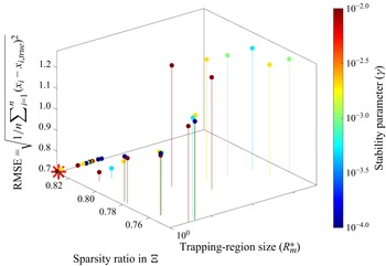


 Open access

