


1. Introduction
Many of the real-world technical items have a random initial age when they are first put into operation. In reliability engineering applications, a failed component is often replaced by either a used component or a spare. The latter usually is not “as good as new” owing to storage or various prior tests such as burn-in performed on many devices before they are put into field operation. Subjects in clinical studies are infected for a random amount of time before enrolling in the study. In population biology and demography, random ages naturally occur when items/organisms are described not only by their associated lifetime distributions but also by their birth rates as functions of the chronological time (see Keyfitz and Caswell [Reference Keyfitz and Caswell10], Finkelstein and Vaupel [Reference Finkelstein and Vaupel6] and the references therein).
The age composition of a population, i.e., the distribution of the random age of an operating item picked up at random from a population at a given chronological time, plays an important role in population studies. This distribution has various applications in different branches of science and engineering including social science, actuarial science and reliability theory. In actuarial science and demography, apart from other implementations, it is used to generate the life/mortality tables that define the one-year survival probabilities for organisms of different ages. In reliability theory, it can be, e.g., used to study the age properties of population of manufactured items such as cars or just of items with a random/unknown initial age.
In this paper, following recent results reported in the literature, we focus on some stochastic properties of dynamic population of items that are produced in sufficiently large quantities and are continuously incepted into operation subject to demand or replacement upon failure. A random sample from this population (or, equivalently, an item drawn at random) at any given time can be described by its random age and the corresponding remaining lifetime. Thus, the reliability study of random age and the remaining lifetime for population of manufactured items can be useful in various real-life decision-making situations (see Finkelstein and Vaupel [Reference Finkelstein and Vaupel6] and Cha and Finkelstein [Reference Cha and Finkelstein3]). Our paper goes further in studying these random quantities in a heterogeneous setup (see later). However, first we briefly discuss the notions of age composition, remaining lifetime and equilibrium distribution in a homogeneous setting.
Let 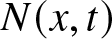 $N(x, t)$ be the age-specific population size at time $t$, representing the number of items of age $x$ at time $t$ (see Keiding [Reference Keiding9] and Arthur and Vaupel [Reference Arthur and Vaupel1]). Furthermore, let an item with random age $X_t$, at time $t$, be drawn at random (with equal chances) from a population of size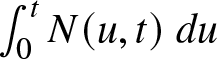 $\int_{0}^{t} N(u, t) \; du$. Then, the “age composition” of this population is represented by the distribution of $X_t$, which is given by the probability density function
 \begin{equation*}\pi_t(x) = \frac{N(x, t)}{\int_{0}^{t}N(u, t) \,du}, \; 0 \leq x \leq t. \end{equation*}
 Furthermore, the corresponding cumulative distribution function of  $X_t$ is given by
 \begin{equation*}\Pi_t(x) = \frac{\int_{0}^{x}N(u, t) \, du}{\int_{0}^{t}N(u, t) \,du}, \; 0 \leq x \leq t. \end{equation*}
See Cha and Finkelstein [Reference Cha and Finkelstein4] for the more detailed discussion of this distribution.
Consider now an item with the lifetime  $T$ that begins to operate at a random (unobserved) age $X$. Then, the remaining lifetime of this item, denoted by $T_X$, is given by
 \begin{equation*}P(T_X \gt t) = \int_{0}^{\infty} \frac{\bar F_T(u+t)}{\bar F_T(u)} \, dF_{X}(u), \; t \gt 0,\end{equation*}
where  $F_X(\cdot)$ and $F_T(\cdot)$ are the cumulative distribution functions of $X$ and $T$, respectively. An important question that can be asked is: what distribution of $X$ is the same as that of $T_X$? In other words, when the initial age is “stochastically” equal to the remaining lifetime? As stated, e.g., in Finkelstein and Vaupel [Reference Finkelstein and Vaupel6], the answer to this query is the solution of the equation
 \begin{equation*}f_X(t) = \int_{0}^{\infty} \frac{f_T(u+t)}{\bar F_T(u)} \, dF_{X}(u) = f_{T_X}(t), \; t \gt 0.\end{equation*}
which is the well-known equilibrium distribution  $f_{X_e}(t)$, defined as
 \begin{equation*}f_{X}(t) = f_{X_e}(t) = \frac{\bar F_T(t)}{\int_{0}^{\infty} \bar F(u) \,du}, \; t \gt 0.\end{equation*}
As discussed previously, the study of different stochastic properties of random age and remaining lifetime for population of manufactured items is useful in different decision-making scenarios. An extensive study on various stochastic comparisons of random ages and remaining lifetimes could be found in the literature, see, for instances, Li and Zuo [Reference Li and Xu14, Reference Li and Zuo15], Cai and Zheng [Reference Cai and Zheng2], Finkelstein and Vaupel [Reference Finkelstein and Vaupel6], Cha and Finkelstein [Reference Cha and Finkelstein3], Hazra et al. [Reference Hazra, Finkelstein and Cha8], Khaledi and Shaked [Reference Khaledi and Shaked12], Dewan and Khaledi [Reference Dewan and Khaledi5] and Patra and Kundu [Reference Patra and Kundu17]. In all the aforementioned studies, it is assumed that the lifetimes of items in a population are independent and identically distributed (i.e., homogeneous population of items). However, in real life items are most often heterogeneous due to various reasons (non-stability of the production process, heterogeneous resources, changing environmental factors, etc.). Recently, Cha and Finkelstein [Reference Cha and Finkelstein4] have introduced the notion of dynamic heterogeneous populations, wherein for modeling heterogeneity, lifetime distributions were indexed by a frailty parameter. For such populations, these authors have considered two types of age compositions: random ages of items obtained by mixing subpopulations with different age distributions and random ages obtained by mixing at the individual items level. The defined age compositions were compared with respect to the likelihood ratio order.
However, in practical scenarios, items may originate from two different populations, raising a natural question: which population yields better-performing items? Furthermore, the remaining lifetime of an item plays a crucial role describing the quality of future performance of items. Despite its practical importance, stochastic comparisons involving the remaining (residual) lifetime and random age in heterogeneous populations were practically not addressed in the literature as well as their ageing properties. We can mention only the paper by Cha and Finkelstein [Reference Cha and Finkelstein4], where some specific comparisons in the sense of the likelihood ratio ordering were obtained, but only for the corresponding age compositions (random ages). These gaps with respect to the remaining lifetime and other stochastic properties in the described set-up motivate the current study.
In this paper, we study some ordering properties of random age and remaining (residual) lifetime for heterogeneous populations of manufactured items. Specifically, we focus on:
• Stochastic comparisons (for random ages of items selected from two different heterogeneous populations) in the sense of hazard rate order, reverse hazard rate order and likelihood ratio order.
• Stochastic comparisons of the random age and remaining lifetime for an item from one heterogeneous population.
• Analyzing stochastic ordering of remaining lifetimes when items from the same generic distribution differ only in their random ages.
• Describing the corresponding ageing properties for both the random age and the residual lifetime in heterogeneous setup.
Our study can be useful for making well-informed choices about, e.g., increasing or decreasing the production rate of items in the manufacturing process or executing the appropriate preventative maintenance actions for a given population.
The rest of the paper is organized as follows. In Section 2, we briefly discuss some preliminaries and useful lemmas. In Section 3, we consider the heterogeneous population of items. In Subsection 3.1, we discuss two different notions of age compositions and compare them stochastically. In Subsection 3.2, we derive some stochastic comparison results between random age and remaining lifetime. Finally, some concluding remarks are made in Section 4.
2. Preliminaries and useful lemmas
Let Z be a random variable with absolutely continuous distribution function  $F_Z(\cdot)$, reliability function $\bar{F}_Z(\cdot) = 1-F_Z(\cdot)$ and probability density function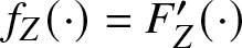 $f_Z(\cdot) = F'_Z(\cdot)$. Furthermore, we denote the set of all real numbers by $\mathbb R$.
The notion of stochastic orders is a very useful tool to compare two or more random variables/vectors. Different types of stochastic orders (namely, the usual stochastic order, the hazard rate order, etc.) have been introduced in the literature to analyze various types of problems in different domains of probability, statistics and allied areas (Shaked and Shanthikumar [Reference Shaked and Shanthikumar18]). In the following, we give the definitions of some stochastic orders that are exclusively used in our paper.
Definition 2.1. Let  $X$ and $Y$ be two absolutely continuous random variables with non-negative supports. Then $X$ is said to be smaller than $Y$ in the
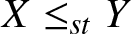
(a) usual stochastic order, denoted by $X\leq_{st}Y$, if
$\bar F_X(x)\leq \bar F_Y(x), \text{for all }x\in~[0,\infty);$
$X\leq_{st}Y$, if
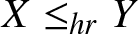
$\bar F_X(x)\leq \bar F_Y(x), \text{for all }x\in~[0,\infty);$(b) hazard rate order, denoted by
$X\leq_{hr}Y$, if
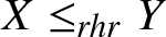
${\bar F_Y(x)}/{\bar F_X(x)}\text{is increasing in } x \in [0,\infty);$(c) reversed hazard rate order, denoted by
$X\leq_{rhr}Y$, if
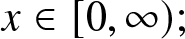
$ {F_Y(x)}/{F_X(x)}\text{is increasing in } $
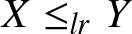
$x\in [0,\infty);$(d) likelihood ratio order, denoted by
$X\leq_{lr}Y$, if
${f_Y(x)}/{f_X(x)}\;\text{is increasing in } x\in(0,\infty);$(e) increasing convex order, denoted by
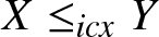
$X\leq_{icx} Y$, if
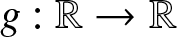
$E (g(X)) \leq E (g(Y ))$ for any increasing and convex function
$g : \mathbb R \rightarrow \mathbb R$.





Similar to stochastic orders, stochastic ageings are extremely useful in describing how a system performs over time. In the literature, various ageing classes (e.g., IFR, DFR, ILR, DLR, etc.) were introduced to characterize different ageing properties of a system (see Lie and Xie [Reference Lai and Xie13]). In the following, we give the definitions of some ageing classes that are used in our paper.
Definition 2.2. Let  $X$ be an absolutely continuous random variable with nonnegative support. Then $X$ is said to have the
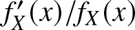
(a) increasing likelihood ratio (ILR) (resp. decreasing likelihood ratio (DLR)) property if
$f_X' (x)/f_X (x)$ is decreasing (resp. increasing) in
$x \gt 0$;(b) increasing failure rate (IFR) (resp. decreasing failure rate (DFR)) property if
$r_X(x)$ is increasing (resp. decreasing) in
$x \gt 0$;(c) decreasing reversed failure rate (DRFR) property if
$r_X (x)$ is decreasing in
$x \gt 0$;(d) decreasing mean residual life (DMRL) (resp. increasing mean residual life (IMRL)) property if
$m_X (x) = E[X - x|X \gt x ]$ is decreasing (resp. increasing) in
$x \gt 0$.




In what follows, we state some lemmas that will be used in proving the main results of this paper.
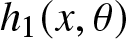
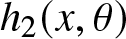
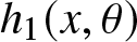
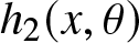
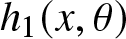
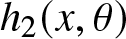
Lemma 2.1. (Lemma 2.4 of Mishra and Naqvi [Reference Misra and Naqvi16]). Let  $h_i(x,\theta):[0,\infty)\times[0,\infty)\rightarrow \mathbb{R}$, i=1,2, be a function, and $g_{i}(\theta)$,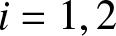 $i=1,2$, be the pdf of the random variable $\Theta_i$, i=1,2. Furthermore, let
 \begin{align*}
K(x)=\frac{\int_{0}^{\infty}h_2(x,\theta)\,dG_2(\theta)}{\int_{0}^{\infty}h_1(x,\theta)\,dG_1(\theta)}, \quad x \gt 0.
\end{align*}
\begin{align*}
K(x)=\frac{\int_{0}^{\infty}h_2(x,\theta)\,dG_2(\theta)}{\int_{0}^{\infty}h_1(x,\theta)\,dG_1(\theta)}, \quad x \gt 0.
\end{align*}Consider the following set of conditions.
(i) Either
$h_1(x,\theta)$ or
$h_2(x,\theta)$ is
$TP_2$ (resp.
$RR_2$) in
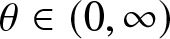
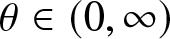
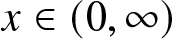
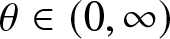
$(x,\theta)\in (0,\infty)\times(0,\infty)$;(ii)
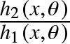
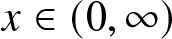
$\frac{h_2(x,\theta)}{h_1(x,\theta)}$ is increasing (resp. decreasing) in
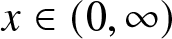
$x\in(0,\infty)$ and is increasing in
$\theta\in(0,\infty)$;(iii) Either
$h_1(x,\theta)$ or
$h_2(x,\theta)$ is increasing in
$\theta\in (0,\infty)$, for all
$x\in (0,\infty)$;(iv) Either
$h_1(x,\theta)$ or
$h_2(x,\theta)$ is decreasing in
$\theta\in (0,\infty)$, for all
$x\in (0,\infty)$;(v)
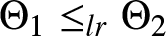
$\Theta_1\leq_{lr}\Theta_2$.(vi)
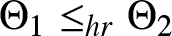
$\Theta_1\leq_{hr}\Theta_2$;(vii)
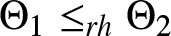
$\Theta_1\leq_{rh}\Theta_2$.



Suppose  $\{(i),(ii),(v)\}$ or $\{(i),(ii),(iii),(vi)\}$ or $\{(i),(ii),(iv),(vii)\}$ holds. Then, $K(x)$ is increasing (resp. decreasing) in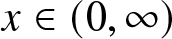 $x\in (0,\infty)$.
Lemma 2.2. (Lemma 2.1 of Hazra and Finkelstein [Reference Hazra and Finkelstein7]). Let 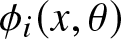 $\phi_i(x,\theta)$, i=1,2, be a nonnegative real valued function on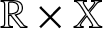 $\mathbb{R}\times \mathbb{X}$, where $\mathbb{R}$ is the set of real numbers, and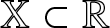 $\mathbb{X}\subset \mathbb{R}$. Suppose the following conditions hold.
(i)
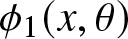
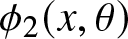
$\phi_1(x,\theta)$ or
$\phi_2(x,\theta)$is
$[TP_2, RR_2, TP_2, RR_2, respectively]$ in
$(x,\theta)\in \mathbb{R}\times\mathbb{X}$;(ii) For
$\theta\in \mathbb{X}$,
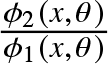
$\frac{\phi_2(x,\theta)}{\phi_1(x,\theta)}$ is [increasing, increasing, decreasing, decreasing, respectively] in
$x\in\mathbb{R}$;(iii) For
$x\in \mathbb{R}$,
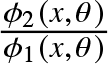
$\frac{\phi_2(x,\theta)}{\phi_1(x,\theta)}$ is [increasing, decreasing, decreasing, increasing, respectively] in
$\theta\in\mathbb{X}$.






Then
 \begin{align*}
S_i(x)=\int_{\mathbb{X}}\phi_i(x,\theta)\,dG(\theta) is \;[TP_2, TP_2, RR_2, RR_2, \text{respectively}] \text{in } (x,i)\in \mathbb{R}\times\{1,2\},
\end{align*}
\begin{align*}
S_i(x)=\int_{\mathbb{X}}\phi_i(x,\theta)\,dG(\theta) is \;[TP_2, TP_2, RR_2, RR_2, \text{respectively}] \text{in } (x,i)\in \mathbb{R}\times\{1,2\},
\end{align*}where  $G(\cdot)$ is a continuous function with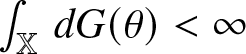 $\int_{\mathbb{X}}\,dG(\theta) \lt \infty$.
3. Main results
In this section, we consider heterogeneous population of items. We discuss two different age compositions and study some stochastic comparison results. Furthermore, we discuss the important role of the equilibrium distribution in obtaining the remaining lifetime of an item with a random initial age.
3.1. Two different age compositions for population of items
In this section, we give the definition of age composition for heterogeneous populations. Then, we derive some stochastic comparisons for the random age of items chosen from two different populations. Recently, Cha and Finkelstein [Reference Cha and Finkelstein4] introduced the notion of dynamic heterogeneous populations wherein the lifetime distributions are indexed by a frailty parameter. Before providing the corresponding definition, we briefly review the context in the homogeneous set-up.
Assume that at time  $t$, items are produced (incepted into operation) at rate $B(t)$. Thus, the total number of items produced in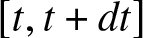 $[t,t + dt]$ is given by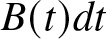 $B(t)dt$. Let items be incepted into operation immediately after being manufactured (as for organisms). Furthermore, let the lifetimes of items manufactured at any time $t\geq 0$, denoted by $T_t$, be independent and identically distributed with the distribution function $F_{T}(\cdot)$. Then, the age composition of an item with random age $X_t$ at time $t$ is defined by
 \begin{align*}
f_{X_t}(x)= \frac{B\left( t-x \right)\bar{F}_{T}\left( x\right) }{\int_{0}^{t}B\left( t-u \right)\bar{F}_{T}\left( u\right)\,du } I\left( 0\leq x \leq t \right),
\end{align*}
\begin{align*}
f_{X_t}(x)= \frac{B\left( t-x \right)\bar{F}_{T}\left( x\right) }{\int_{0}^{t}B\left( t-u \right)\bar{F}_{T}\left( u\right)\,du } I\left( 0\leq x \leq t \right),
\end{align*}where the numerator, multiplied by  $dx$, is the number of items “alive” and having the age $x$ (i.e., in the interval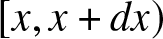 $[x, x + dx)$); the denominator is the size of the population at time $t$, and $I(\cdot)$ is an indicator function. If the manufacturing rate is constant over time, i.e.,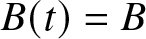 $B(t) = B$ for $t \gt 0$, then the age composition reduces to the density of the equilibrium distribution. We will discuss now these notions for heterogeneous populations for two different scenarios.
Model I: Let the lifetimes of items manufactured at time  $t$ be heterogeneous, as usually the case in practice due to non-stability of the production process, heterogeneous resources, changing environmental factors, etc. This means that the corresponding subpopulations’ distribution functions can be defined as
 \begin{equation*}F_{T_t | \Theta_t = \theta}(x, \theta)= P(T_t \leq x | \Theta_{t} = \theta) = F_{T_t(\theta)}(x, \theta),\end{equation*}
where  $\Theta_t$ is a random variable (frailty), with the probability density function $g_t(\theta)$ with support on $[0, \infty)$, defining variability in the manufactured/incepted items at time $t$;
$t$;  $(T_t| \Theta_{t} = \theta) \stackrel{\rm def}{=} T_t(\theta)$ is the lifetime of an item indexed by $\theta$, and $T_t$ is the lifetime of an item with distribution defined as the following mixture
 \begin{equation*}F_{T_t}(x) = \int_{0}^{\infty}F_{T_t(\theta) }(x, \theta) g_t(\theta) \, d\theta. \end{equation*}
 In this model, the heterogeneity in lifetimes is caused by heterogeneity in production processes. Thus, it is natural to assume that the production rate also depends on  $\theta$, i.e., $B_{\theta}(t)$. Thus, the bivariate extension of the univariate pdf $f_{X_t}(\cdot)$ to the heterogeneous case is given by
 \begin{align*}
f_{X_t | \Theta_t =\theta} (x, \theta)= \frac{B_{\theta}\left( t-x \right)\bar{F}_{T_{t-x}(\theta)}\left( x, \theta\right) }{\int_{0}^{t}B_{\theta}\left( t-u \right)\bar{F}_{T_{t-u}(\theta)}\left( u, \theta\right)\,du } I\left( 0\leq x \leq t \right),
\end{align*}
\begin{align*}
f_{X_t | \Theta_t =\theta} (x, \theta)= \frac{B_{\theta}\left( t-x \right)\bar{F}_{T_{t-x}(\theta)}\left( x, \theta\right) }{\int_{0}^{t}B_{\theta}\left( t-u \right)\bar{F}_{T_{t-u}(\theta)}\left( u, \theta\right)\,du } I\left( 0\leq x \leq t \right),
\end{align*}which represents the age composition at time  $t$ of items belonging to the subpopulation characterized by the frailty variable $\theta$. One may note that the probability density function, $g_{t}(\theta)$, of variability in the manufactured/incepted items at time $t$ can be described via the $\theta$-specific production rate as
 \begin{equation*}g_{t}(\theta) = \frac{B_{\theta}(t)}{\int_{0}^{\infty}B_{\theta}(t)\, d\theta }.\end{equation*}
 Thus, the age composition of an item with random age at time  $t$, denoted by $X_t(\Theta)$, is given by
 \begin{equation}
f_{X_t(\Theta)} (x)= \int_{0}^{\infty}\frac{B_{\theta}\left( t-x \right)\bar{F}_{T_{t-x}(\theta)}\left( x, \theta\right) }{\int_{0}^{t}B_{\theta}\left( t-u \right)\bar{F}_{T_{t-u}(\theta)}\left( u, \theta\right)\,du } g_{t-x}(\theta) \, d\theta, \;0\leq x \leq t .
\end{equation}
\begin{equation}
f_{X_t(\Theta)} (x)= \int_{0}^{\infty}\frac{B_{\theta}\left( t-x \right)\bar{F}_{T_{t-x}(\theta)}\left( x, \theta\right) }{\int_{0}^{t}B_{\theta}\left( t-u \right)\bar{F}_{T_{t-u}(\theta)}\left( u, \theta\right)\,du } g_{t-x}(\theta) \, d\theta, \;0\leq x \leq t .
\end{equation} If 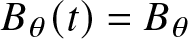 $B_{\theta}(t)= B_{\theta} $ (i.e., does not depend on the chronological time), describing the stability of the production process in time, then the mixing distribution also does not depend on $t$, i.e., $g_{t}(\theta) = g(\theta)$ (or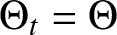 $\Theta_t =\Theta$). Furthermore, if we assume that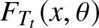 $F_{T_t}(x, \theta)$ also does not depend on the production process in time, i.e., $F_{T_t(\theta)}(x, \theta) = F_{T(\theta)}(x, \theta)$, then the probability density function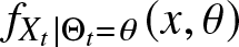 $f_{X_t | \Theta_t =\theta} (x, \theta)$ reduces to
 \begin{align*}
f_{X_t | \Theta_t =\theta} (x, \theta)= \frac{\bar{F}_{T(\theta)}\left( x, \theta\right) }{\int_{0}^{t}\bar{F}_{T(\theta)}\left( u, \theta\right)\,du } I\left( 0\leq x \leq t \right),
\end{align*}
\begin{align*}
f_{X_t | \Theta_t =\theta} (x, \theta)= \frac{\bar{F}_{T(\theta)}\left( x, \theta\right) }{\int_{0}^{t}\bar{F}_{T(\theta)}\left( u, \theta\right)\,du } I\left( 0\leq x \leq t \right),
\end{align*} For the sake of simplicity of the notation, we omit the subscript  $T(\theta)$ in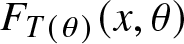 $F_{T(\theta)}(x, \theta)$. Thus, the age composition of an item with random age at time $t$, denoted by $Y_{t}(\Theta)$, is given by
 \begin{equation}
f_{Y_t(\Theta)} (x)=\int_{0}^{\infty} f_{Y_t | \Theta_t =\theta} (x, \theta) g(\theta) \;d\theta = \int_{0}^{\infty} \frac{\bar{F}\left( x, \theta\right) }{\int_{0}^{t}\bar{F}\left( u, \theta\right)\,du } g(\theta) \,d\theta, \; 0\leq x \leq t.
\end{equation}
\begin{equation}
f_{Y_t(\Theta)} (x)=\int_{0}^{\infty} f_{Y_t | \Theta_t =\theta} (x, \theta) g(\theta) \;d\theta = \int_{0}^{\infty} \frac{\bar{F}\left( x, \theta\right) }{\int_{0}^{t}\bar{F}\left( u, \theta\right)\,du } g(\theta) \,d\theta, \; 0\leq x \leq t.
\end{equation} Note that, 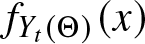 $f_{Y_t(\Theta)} (x)$ is the unconditional expectation of the subpopulation age compositions with respect to the frailty distribution $ g(\theta)$. By definition, $ g(\theta)$ describes the proportion of items with frailty $\theta$ at the time of production. However, this does not coincide with the actual proportion of such items in the population at a later time, since items from different subpopulations experience different failure probabilities and some have already failed. Consequently, although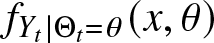 $f_{Y_t | \Theta_t =\theta} (x, \theta)$ represents the true age composition of the subpopulation indexed by $\theta$, the resulting distribution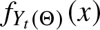 $f_{Y_t(\Theta)} (x)$ may not correspond to the real age composition of the heterogeneous population at time $t$. However, this distribution coincides with the true age composition under restrictive conditions, namely when all subpopulations are statistically identical or when items produced according to $ g(\theta)$ do not experience failures. Furthermore, the age composition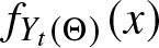 $f_{Y_t(\Theta)} (x)$ also has another practical interpretation when mixing is performed at a different level and arises from a different origin (see Cha and Finkelstein [Reference Cha and Finkelstein4]).
To obtain the heterogeneous population, instead of mixing the age compositions of subpopulations as in Model I, we mix at the level of an individual item. In this way, the resulting age composition, defined through the intrinsic heterogeneity of the population, can be interpreted similarly to the expectation of 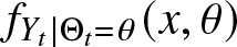 $f_{Y_t | \Theta_t =\theta} (x, \theta)$ in Model I, but with respect to a different probability density function.
Model II: Let the heterogeneous population be modeled not by mixing age compositions of subpopulations but by “mixing on the level of an item.” Thus, the age composition of an item with random age at time  $t$, denoted by $\tilde X_{t}(\Theta)$, is given by
 \begin{equation}
f_{\tilde X_t(\Theta)} (x)=\frac{\int_{0}^{\infty}B_{\theta}\left( t-x \right)\bar{F}_{T_{t-x}(\theta)}\left( x, \theta\right) g_{t-x}(\theta) \, d\theta }{\int_{0}^{t} \int_{0}^{\infty}B_{\theta}\left( t-u \right)\bar{F}_{T_{t-u}(\theta)}\left( u, \theta\right) g_{t-u}(\theta)\,d\theta \, du }.
\end{equation}
\begin{equation}
f_{\tilde X_t(\Theta)} (x)=\frac{\int_{0}^{\infty}B_{\theta}\left( t-x \right)\bar{F}_{T_{t-x}(\theta)}\left( x, \theta\right) g_{t-x}(\theta) \, d\theta }{\int_{0}^{t} \int_{0}^{\infty}B_{\theta}\left( t-u \right)\bar{F}_{T_{t-u}(\theta)}\left( u, \theta\right) g_{t-u}(\theta)\,d\theta \, du }.
\end{equation} In particular, if 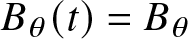 $B_{\theta}(t)= B_{\theta} $ and $F_{T_t(\theta)}(x, \theta) = F(x, \theta)$, for $t \gt 0$, then the age composition of an item with random age at time $t$, denoted by $\tilde Y_{t}(\Theta)$, is given by
 \begin{equation}
f_{\tilde Y_t(\Theta)} (x)=\frac{\int_{0}^{\infty}\bar F(x, \theta) g(\theta) \; d\theta }{\int_{0}^{t} \int_{0}^{\infty}\bar F(u, \theta) g(\theta)\,d\theta \, du }.
\end{equation}
\begin{equation}
f_{\tilde Y_t(\Theta)} (x)=\frac{\int_{0}^{\infty}\bar F(x, \theta) g(\theta) \; d\theta }{\int_{0}^{t} \int_{0}^{\infty}\bar F(u, \theta) g(\theta)\,d\theta \, du }.
\end{equation}In what follows, we discuss the main results of this section. In the following theorem, we compare the random ages of items taken from two different heterogeneous populations by mixing age compositions of subpopulations (i.e., population generated from Model I).
Theorem 3.1 Suppose the following conditions hold.
(i)
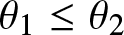
$T(\theta_1) \leq_{hr}(\text{resp. } \geq_{hr}) \;T(\theta_2)$, whenever
$\theta_1 \leq \theta_2$;(ii)
$\Theta_1 \leq_{[lr, hr, rh]}(\text{resp. } \leq_{[lr, rh, hr]})\; \Theta_2$.


Then  $Y_u\left(\Theta_1\right) \leq_{[lr, hr, rh]}(\text{resp. }\geq_{[lr, hr, rh]})\; Y_u\left(\Theta_2\right)$.
Proof. We prove the result for the likelihood ratio order and the hazard rate order. The proof for the reverse hazard order follows in the same line and is, therefore, omitted. We first proceed to prove the result for the likelihood ratio order. From (3.2), we get
 \begin{align*}
f_{Y_u(\Theta_1)}(t) = \int_{0}^{\infty} \frac{\bar{F}(t | \theta)}{\int_{0}^{u}\bar{F}(w | \theta) \,dw} g_1(\theta) \,d \theta, \quad 0 \leq t \leq u,
\end{align*}
\begin{align*}
f_{Y_u(\Theta_1)}(t) = \int_{0}^{\infty} \frac{\bar{F}(t | \theta)}{\int_{0}^{u}\bar{F}(w | \theta) \,dw} g_1(\theta) \,d \theta, \quad 0 \leq t \leq u,
\end{align*}and
 \begin{align*}
f_{Y_u(\Theta_2)}(t) = \int_{0}^{\infty} \frac{\bar{F}(t | \theta)}{\int_{0}^{u}\bar{F}(w | \theta) \,dw} g_2(\theta) \,d \theta, \quad 0 \leq t \leq u.
\end{align*}
\begin{align*}
f_{Y_u(\Theta_2)}(t) = \int_{0}^{\infty} \frac{\bar{F}(t | \theta)}{\int_{0}^{u}\bar{F}(w | \theta) \,dw} g_2(\theta) \,d \theta, \quad 0 \leq t \leq u.
\end{align*}Thus, to prove the result, it suffices to show that
 \begin{equation}
\frac{f_{Y_u(\Theta_2)}(t)}{f_{Y_u(\Theta_1)}(t)} \text{is increasing (resp. decreasing) in } 0 \leq t \leq u.
\end{equation}
\begin{equation}
\frac{f_{Y_u(\Theta_2)}(t)}{f_{Y_u(\Theta_1)}(t)} \text{is increasing (resp. decreasing) in } 0 \leq t \leq u.
\end{equation} Now, from condition  $(i)$, we get that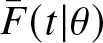 $\bar{F} (t | \theta)$ is $TP_2$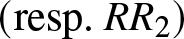 $( \text{resp. } RR_2)$ in $(t, \theta) \in [0, u] \times [0, \infty)$, which further implies that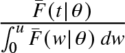 $\frac{\bar{F}(t | \theta)}{\int_{0}^{u}\bar{F}(w | \theta) \,dw}$ is $TP_2$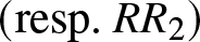 $( \text{resp. } RR_2)$ in $(t, \theta) \in [0, u] \times [0, \infty)$. Therefore, by using condition $(ii)$ in Lemma 2.1, we get (3.5). Hence, the result is proved for the likelihood ratio order. Next, we proceed to prove the result for the hazard rate order. From (3.2), we have
 \begin{align*}
\bar F_{Y_u(\Theta_1)}(t) =\int_{0}^{\infty} k_1(t | \theta)g_1(\theta) \,d \theta,\quad 0 \leq t \leq u,
\end{align*}
\begin{align*}
\bar F_{Y_u(\Theta_1)}(t) =\int_{0}^{\infty} k_1(t | \theta)g_1(\theta) \,d \theta,\quad 0 \leq t \leq u,
\end{align*}and
 \begin{align*}
\bar F_{Y_u(\Theta_2)}(t) = \int_{0}^{\infty} k_1( t | \theta ) g_2(\theta) \,d \theta, \quad 0 \leq t \leq u,
\end{align*}
\begin{align*}
\bar F_{Y_u(\Theta_2)}(t) = \int_{0}^{\infty} k_1( t | \theta ) g_2(\theta) \,d \theta, \quad 0 \leq t \leq u,
\end{align*}where
 \begin{equation*}k_1( t | \theta) = \frac{\int_{t}^{u}\bar{F}(w | \theta) \, dw}{\int_{0}^{u}\bar{F}(w | \theta) \,dw}, \quad 0 \leq t \leq u.\end{equation*}
Thus, to prove the result, it suffices to show that
 \begin{equation}
\frac{\bar F_{Y_u(\Theta_2)}(t)}{\bar F_{Y_u(\Theta_1)}(t)} \text{is increasing (resp. decreasing) in } 0 \leq t \leq u.
\end{equation}
\begin{equation}
\frac{\bar F_{Y_u(\Theta_2)}(t)}{\bar F_{Y_u(\Theta_1)}(t)} \text{is increasing (resp. decreasing) in } 0 \leq t \leq u.
\end{equation}Now, we can write
 \begin{align*}
\int_{t}^{u}\bar{F}(w | \theta) \, dw = \int_{0}^{u} n_1(t, w) \bar{F}(w | \theta) \, dw , \quad 0 \leq t \leq u,
\end{align*}
\begin{align*}
\int_{t}^{u}\bar{F}(w | \theta) \, dw = \int_{0}^{u} n_1(t, w) \bar{F}(w | \theta) \, dw , \quad 0 \leq t \leq u,
\end{align*}where
 \begin{equation*}
n_1(t, w) =
\begin{cases}
1 & \text{if}~t \leq w\\
0 & \text{otherwise.}
\end{cases}
\end{equation*}
\begin{equation*}
n_1(t, w) =
\begin{cases}
1 & \text{if}~t \leq w\\
0 & \text{otherwise.}
\end{cases}
\end{equation*} From condition  $(i)$, we get that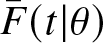 $\bar{F} (t | \theta)$ is $TP_2$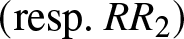 $( \text{resp. } RR_2)$ in $(t, \theta) \in [0, u] \times [0, \infty)$. Furthermore, note that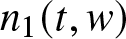 $n_1 (t, w)$ is $TP_2$ in $(t, w) \in [0, u] \times [0, u]$. Consequently, we get that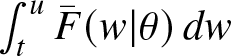 $\int_{t}^{u}\bar{F}(w | \theta) \, dw$ is $TP_2$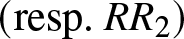 $( \text{resp. } RR_2)$ in $(t, \theta) \in [0, u] \times [0, \infty)$, which further implies that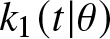 $k_1(t | \theta)$ is $TP_2$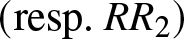 $( \text{resp. } RR_2)$ in $(t, \theta) \in [0, u] \times [0, \infty)$ and is increasing (resp. decreasing) in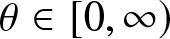 $\theta \in [0, \infty)$. Finally, by using these and condition $(ii)$ in Lemma 2.1, we get (3.6). Hence, the result is proved for the hazard rate order. □
In the next theorem, we compare the random ages of items taken from two different heterogeneous populations by mixing on the level of an item (i.e., population generated from Model II).
Theorem 3.2 Suppose the following conditions hold.
(i)
$T(\theta_1) \leq_{hr}(\text{resp. }\geq_{hr}) \;T(\theta_2)$, whenever
$\theta_1 \leq \theta_2$;(ii)
$\Theta_1 \leq_{[lr, hr]} (\text{resp. }\leq_{[lr, rh]}) \;\Theta_2$.

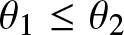

Then  $\tilde Y_u\left(\Theta_1\right) \leq_{[lr, hr]}(\text{resp. }\geq_{[lr, hr]}) \;\tilde Y_u\left(\Theta_2\right)$.
Proof. We first proceed to prove the result for the likelihood ratio order. From (3.4), we get
 \begin{align*}
f_{\tilde Y_u(\Theta_1)}(t) = \int_{0}^{\infty} \frac{\bar{F}(t | \theta)}{\int_{0}^{u}\bar{F}(w | \theta) \,dw} g^{*}_1(\theta) \,d \theta, \quad 0 \leq t \leq u,
\end{align*}
\begin{align*}
f_{\tilde Y_u(\Theta_1)}(t) = \int_{0}^{\infty} \frac{\bar{F}(t | \theta)}{\int_{0}^{u}\bar{F}(w | \theta) \,dw} g^{*}_1(\theta) \,d \theta, \quad 0 \leq t \leq u,
\end{align*}and
 \begin{align*}
f_{\tilde Y_u(\Theta_2)}(t) = \int_{0}^{\infty} \frac{\bar{F}(t | \theta)}{\int_{0}^{u}\bar{F}(w | \theta) \,dw} g^{*}_2(\theta) \,d \theta, \quad 0 \leq t \leq u,
\end{align*}
\begin{align*}
f_{\tilde Y_u(\Theta_2)}(t) = \int_{0}^{\infty} \frac{\bar{F}(t | \theta)}{\int_{0}^{u}\bar{F}(w | \theta) \,dw} g^{*}_2(\theta) \,d \theta, \quad 0 \leq t \leq u,
\end{align*}where
 \begin{equation*}g^{*}_i(\theta) = \frac{\int_{0}^{u}\bar{F}(w | \theta) \,dw g_i(\theta)}{\int_{0}^{u} \int_{0}^{\infty} \bar{F}(w | \theta) g_i(\theta)\,d\theta \,dw}\end{equation*}
is the probability density function of a random variable  $\Theta_i^{*}$ (say),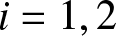 $i=1,2$. Thus, to prove the result, it is suffices to show that
 \begin{equation}
\frac{f_{\tilde Y_u(\Theta_2)}(t)}{f_{\tilde Y_u(\Theta_1)}(t)} \text{is increasing (resp. decreasing) in } 0 \leq t \leq u.
\end{equation}
\begin{equation}
\frac{f_{\tilde Y_u(\Theta_2)}(t)}{f_{\tilde Y_u(\Theta_1)}(t)} \text{is increasing (resp. decreasing) in } 0 \leq t \leq u.
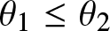
\end{equation} Now, from condition  $(i)$, we get that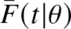 $\bar{F} (t | \theta)$ is $TP_2$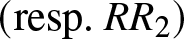 $( \text{resp. } RR_2)$ in $(t, \theta) \in [0, u] \times [0, \infty)$, which further implies that ${\bar{F}(t | \theta)}/{\int_{0}^{u}\bar{F}(w | \theta) \,dw}$ is $TP_2$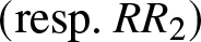 $( \text{resp. } RR_2)$ in $(t, \theta) \in [0, u] \times [0, \infty)$. Again, from condition $(ii)$, we get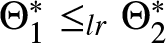 $\Theta^{*}_1 \leq_{lr} \Theta^{*}_2 $. Then, by using Lemma 2.1, we get (3.7). Hence, the result is proved for the likelihood ratio order. Next, we proceed to prove the result for the hazard rate order. From (3.4), we get
 \begin{align*}
\bar F_{\tilde Y_u(\Theta_1)}(t)
=\int_{0}^{\infty} \psi_1(t | \theta)g^{*}_1(\theta) \,d \theta,\quad 0 \leq t \leq u,
\end{align*}
\begin{align*}
\bar F_{\tilde Y_u(\Theta_1)}(t)
=\int_{0}^{\infty} \psi_1(t | \theta)g^{*}_1(\theta) \,d \theta,\quad 0 \leq t \leq u,
\end{align*}and
 \begin{align*}
\bar F_{\tilde Y_u(\Theta_2)}(t) = \int_{0}^{\infty} \psi_1( t | \theta ) g^{*}_2(\theta) \,d \theta, \quad 0 \leq t \leq u,
\end{align*}
\begin{align*}
\bar F_{\tilde Y_u(\Theta_2)}(t) = \int_{0}^{\infty} \psi_1( t | \theta ) g^{*}_2(\theta) \,d \theta, \quad 0 \leq t \leq u,
\end{align*}where
 \begin{equation*}\psi_1( t | \theta) = \frac{\int_{t}^{u}\bar{F}(w | \theta) \, dw}{\int_{0}^{u}\bar{F}(w | \theta) \,dw},\quad 0 \leq t \leq u,\end{equation*}
and
 \begin{equation*}g^{*}_i(\theta) = \frac{\int_{0}^{u}\bar{F}(w | \theta) \,dw g_i(\theta)}{\int_{0}^{\infty} \int_{0}^{u}\bar{F}(w | \theta) g_i(\theta) \; dw \;d \theta}\end{equation*}
is the probability density function of a random variable  $\Lambda_i^{*}$,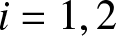 $i=1,2$. Thus, to prove the result, it is suffices to show that
 \begin{equation}
\frac{\bar F_{\tilde Y_u(\Theta_2)}(t)}{\bar F_{\tilde Y_u(\Theta_1)}(t)} \text{is increasing (resp. decreasing) in } 0 \leq t \leq u.
\end{equation}
\begin{equation}
\frac{\bar F_{\tilde Y_u(\Theta_2)}(t)}{\bar F_{\tilde Y_u(\Theta_1)}(t)} \text{is increasing (resp. decreasing) in } 0 \leq t \leq u.
\end{equation}Now, we can write
 \begin{align*}
\int_{t}^{u}\bar{F}(w | \theta) \, dw = \int_{0}^{u} n_1(t, w) \bar{F}(w | \theta) \, dw , \quad 0 \leq t \leq u,
\end{align*}
\begin{align*}
\int_{t}^{u}\bar{F}(w | \theta) \, dw = \int_{0}^{u} n_1(t, w) \bar{F}(w | \theta) \, dw , \quad 0 \leq t \leq u,
\end{align*}where
 \begin{equation*}
n_1(t, w) =
\begin{cases}
1 & \text{if} t \leq w\\
0 & \text{otherwise.}
\end{cases}
\end{equation*}
\begin{equation*}
n_1(t, w) =
\begin{cases}
1 & \text{if} t \leq w\\
0 & \text{otherwise.}
\end{cases}
\end{equation*} From condition  $(i)$, we get that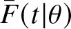 $\bar{F} (t | \theta)$ is $TP_2$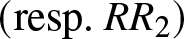 $( \text{resp. } RR_2)$ in $(t, \theta) \in [0, u] \times [0, \infty)$. Furthermore, note that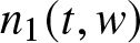 $n_1 (t, w)$ is $TP_2$ in $(t, w) \in [0, u] \times [0, u]$. Consequently, we get that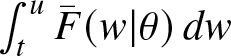 $\int_{t}^{u}\bar{F}(w | \theta) \, dw$ is $TP_2$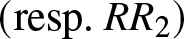 $( \text{resp. } RR_2)$ in $(t, \theta) \in [0, u] \times [0, \infty)$, which further implies that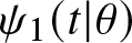 $\psi_1(t | \theta)$ is $TP_2$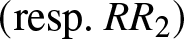 $( \text{resp. } RR_2)$ in $(t, \theta) \in [0, u] \times [0, \infty)$ and is increasing (resp. decreasing) in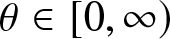 $\theta \in [0, \infty)$. Again, from condition $(i)$, we get that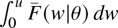 $\int_{0}^{u}\bar{F}(w | \theta) \,dw$ is increasing (resp. decreasing) in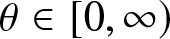 $\theta \in [0, \infty)$. Then, from condition $(ii)$, we get that $\Lambda^{*}_1 \leq_{hr} (\text{resp. } \leq_{rh})\Lambda^{*}_2 $. Consequently, the statement given in (3.8) follows from Lemma 2.1. Hence, the result is proved for the hazard rate order. □
In the following theorem, we compare the random ages of items taken from two different populations (i.e., generated from Models I and II). Here, we assume that the random lifetime (generic) of an item of a subpopulation does not depend on the calendar time  $t$, i.e., $\bar F_{T_t}(x, \theta) = \bar F (x, \theta)$ and the mixing distribution does not depend on $t$, i.e.,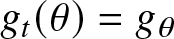 $g_t(\theta ) = g_{\theta}$.
Theorem 3.3 Suppose the following conditions hold.
(i)
$T(\theta_1) \leq_{hr}(\text{resp. }\geq_{hr})\; T(\theta_2)$, whenever
$\theta_1 \leq \theta_2$;(ii)
$B_{\theta} (t)$ is
$RR_2$
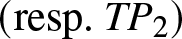
$ (\text{resp. } TP_2)$ in
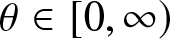
$(t, \theta) \in [0, \infty) \times [0, \infty)$ and is increasing (resp. decreasing) in
$\theta \in[0, \infty)$.




Then,  $X_u\left(\Theta\right) \leq_{lr} \tilde X_u\left(\Theta\right)$.
Proof. From (3.1) and (3.3), we have
 \begin{align*}
f_{X_u(\Theta)}(t) = \int_{0}^{\infty} \frac{B_{\theta}(u-t) \bar{F}(t | \theta)}{\int_{0}^{u} B_{\theta}(u-w) \bar{F}(w | \theta) \,dw} g(\theta) \,d \theta, \quad 0 \leq t \leq u,
\end{align*}
\begin{align*}
f_{X_u(\Theta)}(t) = \int_{0}^{\infty} \frac{B_{\theta}(u-t) \bar{F}(t | \theta)}{\int_{0}^{u} B_{\theta}(u-w) \bar{F}(w | \theta) \,dw} g(\theta) \,d \theta, \quad 0 \leq t \leq u,
\end{align*}and
 \begin{align*}
f_{\tilde X_u(\Theta)}(t)= \int_{0}^{\infty} \frac{B_{\theta}(u-t) \bar{F}(t | \theta)}{\int_{0}^{u} B_{\theta}(u-w) \bar{F}(w | \theta) \,dw} g^{*}(\theta) \,d \theta, \quad 0 \leq t \leq u,
\end{align*}
\begin{align*}
f_{\tilde X_u(\Theta)}(t)= \int_{0}^{\infty} \frac{B_{\theta}(u-t) \bar{F}(t | \theta)}{\int_{0}^{u} B_{\theta}(u-w) \bar{F}(w | \theta) \,dw} g^{*}(\theta) \,d \theta, \quad 0 \leq t \leq u,
\end{align*}where
 \begin{equation*}g^{*}(\theta) = \frac{\int_{0}^{u}B_{\theta}(u-w) \bar{F}(w | \theta) \,dw g(\theta)}{\int_{0}^{\infty} \int_{0}^{u}B_{\theta}(u-w) \bar{F}(w | \theta) g(\theta) \,dw \,d\theta}\end{equation*}
is the probability density function of a random variable, say,  $\Theta^*$. Thus, to prove the result, it suffices to show that
 \begin{equation}
\frac{f_{\tilde X_u(\Theta)}(t)}{f_{X_u(\Theta)}(t)} \text{is increasing in } 0 \leq t \leq u.
\end{equation}
\begin{equation}
\frac{f_{\tilde X_u(\Theta)}(t)}{f_{X_u(\Theta)}(t)} \text{is increasing in } 0 \leq t \leq u.
\end{equation} Now, from conditions  $(i)$ and $(ii)$, we get that $B_{\theta}(u-t) \bar{F} (t | \theta)$ is increasing (resp. decreasing) in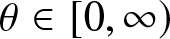 $\theta \in [0, \infty)$. Furthermore, this implies that
 \begin{equation}
\Theta \leq_{lr} (\text{resp. } \geq_{lr}) \Theta^{*}.
\end{equation}
\begin{equation}
\Theta \leq_{lr} (\text{resp. } \geq_{lr}) \Theta^{*}.
\end{equation} Again, from conditions  $(i)$ and $(ii)$, we get that $B_{\theta}(u-t) \bar{F} (t | \theta)$ is $TP_2$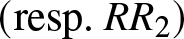 $( \text{resp. } RR_2)$ in $(t, \theta) \in [0, u] \times [0, \infty)$, which further implies that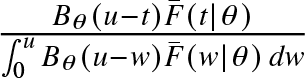 $\frac{B_{\theta}(u-t)\bar{F}(t | \theta)}{\int_{0}^{u} B_{\theta}(u-w)\bar{F}(w | \theta) \,dw}$ is $TP_2$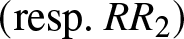 $( \text{resp. } RR_2)$ in $(t, \theta) \in [0, u] \times [0, \infty)$. Finally, by using this and (3.10) in Lemma 2.1, we get (3.9). Hence, the result is proved. □
In the following example, we demonstrate the result given in Theorem 3.1.
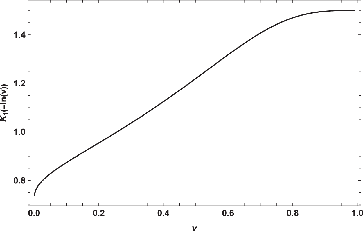
Example 3.1. Consider two different items with random ages 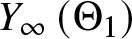 $Y_{\infty}\left(\Theta_1\right)$ and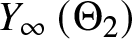 $Y_{\infty}\left(\Theta_2\right)$, respectively, where $\bar F(t, \theta) = e^{-(\theta t)^3}$, $t \gt 0$, and $g_1(\theta) = 3 e^{-3\theta}$ and $g_2(\theta) = 2 e^{-2\theta}$, $\theta \gt 0$. It can be easily verified that all conditions of Theorem 3.1 are satisfied. Furthermore, let
 \begin{align*}
K_1(t) =\frac{f_{Y_{\infty}\left(\Theta_2\right)}(t) }{f_{Y_{\infty}\left(\Theta_1\right)}(t) } , \quad t \gt 0.
\end{align*}
\begin{align*}
K_1(t) =\frac{f_{Y_{\infty}\left(\Theta_2\right)}(t) }{f_{Y_{\infty}\left(\Theta_1\right)}(t) } , \quad t \gt 0.
\end{align*} By plotting 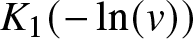 $K_{1}(-\ln(v))$ against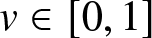 $ v\in[0,1]$ in Figure 1, we see that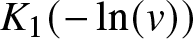 $K_1(-\ln(v))$ is increasing in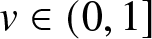 $v\in(0,1]$ and so, $K_1(t)$ is decreasing in $t \gt 0$. Thus, $Y_{\infty}\left(\Theta_1\right) \geq_{lr}\; Y_{\infty}\left(\Theta_2\right)$.
Plot of 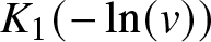 $K_{1}(-\ln(v))$ against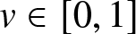 $ v\in[0,1]$.

3.2. Remaining lifetime for population of items
In this section, we establish some stochastic comparisons between random age and remaining lifetime of an item from a heterogeneous population. In the following, we define the notions of the remaining lifetime and the equilibrium distribution for heterogeneous populations.
Consider a heterogeneous population wherein subpopulations are indexed by the random variable  $\Theta$. Let $T(\theta)$ be the lifetime of an item, drawn from a subpopulation indexed by “ $\Theta=\theta$,” having the PDF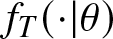 $f_{T}(\cdot| \theta)$ and the reliability function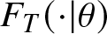 $F_{T}(\cdot| \theta)$. Let this item start operating at a random (unobserved) age $X(\theta)$. Furthermore, let $T_X(\theta)$ be the remaining lifetime of this item. Then, its distribution is given by
 \begin{equation*}P(T_X(\theta) \gt t) = \int_{0}^{\infty} \frac{\bar F_T(u+t| \theta)}{\bar F_T(u| \theta)} f_{X}(u| \theta) \, du, \; t \gt 0,\end{equation*}
where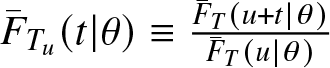 $\bar F_{T_{u}}(t| \theta ) \equiv \frac{\bar F_T(u+t | \theta)}{\bar F_T(u| \theta)}$, $x \gt 0$, is the reliability function of a random variable $T_u(\theta)$, representing the remaining lifetime of the item at a given time $u$, and $f_{X(\theta)}(\cdot)\equiv f_X(\cdot | \theta)$ is the probability density function of $X(\theta)$. Consequently, the remaining lifetime of an item (denoted by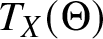 $T_X(\Theta)$), drawn from a heterogeneous population with subpopulations indexed by $\Theta$, has the distribution given by
 \begin{equation}
\bar F_{T_{X}(\Theta)} (t)=\int_{0}^{\infty} \int_{0}^{\infty} \frac{\bar F_T(u+t| \theta)}{\bar F_T(u| \theta)} f_{X}(u|\theta) g(\theta)\, du \, d\theta, \; t \gt 0.
\end{equation}
\begin{equation}
\bar F_{T_{X}(\Theta)} (t)=\int_{0}^{\infty} \int_{0}^{\infty} \frac{\bar F_T(u+t| \theta)}{\bar F_T(u| \theta)} f_{X}(u|\theta) g(\theta)\, du \, d\theta, \; t \gt 0.
\end{equation} Like in the homogeneous case, one important question here is: What distribution of  $X(\Theta)$ results in the identical distribution of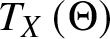 $T_{X}\left( \Theta\right)$? In other words, what is the solution to the following equation:
 \begin{equation}
f_{X(\Theta)} (t)=\int_{0}^{\infty} \int_{0}^{\infty} \frac{f_T(u+t| \theta)}{\bar F_T(u| \theta)} f_{X}(u| \theta) g(\theta)\, du \, d\theta \;\left( = f_{T_{X}(\Theta)} (t)\right), \; \text{for all } t \gt 0.
\end{equation}
\begin{equation}
f_{X(\Theta)} (t)=\int_{0}^{\infty} \int_{0}^{\infty} \frac{f_T(u+t| \theta)}{\bar F_T(u| \theta)} f_{X}(u| \theta) g(\theta)\, du \, d\theta \;\left( = f_{T_{X}(\Theta)} (t)\right), \; \text{for all } t \gt 0.
\end{equation} Note that finding the solution of the above equation is equivalent to obtaining the solution for the case  $\Theta=\theta$, i.e., obtaining the solution of the equation
 \begin{equation}
f_{X(\theta)} (t)=\int_{0}^{\infty} \frac{f_T(u+t |\theta)}{\bar F_T(u| \theta)} f_{X(\theta)}(u)\, du, \; \text{for all } t \gt 0.
\end{equation}
\begin{equation}
f_{X(\theta)} (t)=\int_{0}^{\infty} \frac{f_T(u+t |\theta)}{\bar F_T(u| \theta)} f_{X(\theta)}(u)\, du, \; \text{for all } t \gt 0.
\end{equation} Similar to the homogeneous case, it can be easily verified that the solution of the above equation is the equilibrium distribution, i.e.,  $ f_{X(\theta)}(t) = f_{X_e(\theta)}(t)$, $t \gt 0$, where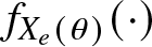 $ f_{X_e(\theta)}(\cdot)$ is the probability density function of the equilibrium distribution given by
 \begin{align*}
f_{X_e(\theta)}(t)= \frac{\bar F_T(t| \theta)}{\int_{0}^{\infty} \bar F_T(u| \theta) \,du}, \; t \gt 0.
\end{align*}
\begin{align*}
f_{X_e(\theta)}(t)= \frac{\bar F_T(t| \theta)}{\int_{0}^{\infty} \bar F_T(u| \theta) \,du}, \; t \gt 0.
\end{align*} Consequently, as the mixture distribution is defined as the corresponding integral with respect to the density of the frailty  $=\theta$, the solution of the original Equation (3.12) is the distribution, which is a mixture of the equilibrium distributions, and it is given by
 \begin{equation}
f_{X_e(\Theta)}(t)= \int_{0}^{\infty} f_{X_e(\theta)}(t)g(\theta)d\theta.
\end{equation}
\begin{equation}
f_{X_e(\Theta)}(t)= \int_{0}^{\infty} f_{X_e(\theta)}(t)g(\theta)d\theta.
\end{equation}As we have seen, the random age of an item from a heterogeneous population is the average of the random ages of the corresponding subpopulations. Furthermore, the remaining lifetime of an item drawn from a heterogeneous population is also the average of the remaining lifetimes of the corresponding subpopulations. Similarly, it is quite natural to consider the equilibrium distribution for a heterogeneous population to be the average of the equilibrium distributions of the corresponding subpopulations.
In what follows, we summarize the above discussion by stating an important result.
Proposition 3.1. If 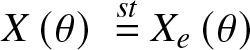 $X(\theta)\;\overset{\text{st}}{=}\;X_e(\theta)$, for all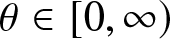 $\theta \in [0, \infty)$, then $X_{e}\left( \Theta\right) \; \overset{st}{=} \; T_{X_e}\left( \Theta\right).$ □
In the preceding proposition, we show that the random age and the remaining lifetime of an item in a heterogeneous population are stochastically the same when the random age distribution in each subpopulation is equal to the equilibrium distribution of the same subpopulation. Then, another natural question arises, which is: When can we say that the remaining lifetime of an item in a heterogeneous population is stochastically larger (or smaller) than its random age? In the next three theorems, we answer this question by obtaining the corresponding stochastic orderings.
Theorem 3.4 Suppose the following conditions hold true.
(i)
$X\left(\theta\right) \; \leq_{st} (\text{resp. } \geq_{st}) \; X_e\left(\theta\right)$, for all
$\theta \in [0, \infty)$;(ii)
$T\left(\theta \right) $ is IFR, for all
$\theta \in [0, \infty)$.

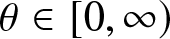

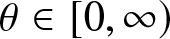
Then  ${X}\left(\Theta\right) \; \leq_{st} (\text{resp. } \geq_{st}) \; T_{X}\left(\Theta\right)$.
Proof. We only prove the result under the condition that  $X\left(\theta\right) \; \leq_{st} \; X_e\left(\theta\right)$. The proof for the other case can be done in the same line. Now, from (3.14) and (3.11), we get
 \begin{align*}
\bar{F}_{{X_e}\left( \Theta \right)} \left( t\right) = \int_{0}^{\infty} \int_{0}^{\infty} \frac{\bar{F}_T \left( t+u | \theta \right) } {\bar{F}_T \left( u | \theta \right) } f_{X_e}\left( u | \theta \right) g\left( \theta\right)\; du \; d\theta, \quad t \gt 0,
\end{align*}
\begin{align*}
\bar{F}_{{X_e}\left( \Theta \right)} \left( t\right) = \int_{0}^{\infty} \int_{0}^{\infty} \frac{\bar{F}_T \left( t+u | \theta \right) } {\bar{F}_T \left( u | \theta \right) } f_{X_e}\left( u | \theta \right) g\left( \theta\right)\; du \; d\theta, \quad t \gt 0,
\end{align*}and
 \begin{align*}
\bar{F}_{T_{X}\left( \Theta\right)} \left( t\right) = \int_{0}^{\infty} \int_{0}^{\infty} \frac{\bar{F}_T \left( t+u | \theta \right) } {\bar{F}_T \left( u | \theta \right) } f_{X}\left( u | \theta \right) g\left( \theta\right)\; du \; d\theta, \quad t \gt 0,
\end{align*}
\begin{align*}
\bar{F}_{T_{X}\left( \Theta\right)} \left( t\right) = \int_{0}^{\infty} \int_{0}^{\infty} \frac{\bar{F}_T \left( t+u | \theta \right) } {\bar{F}_T \left( u | \theta \right) } f_{X}\left( u | \theta \right) g\left( \theta\right)\; du \; d\theta, \quad t \gt 0,
\end{align*}respectively. From condition  $(i)$, we have $X\left(\Theta\right) \leq_{st} X_{e} \left( \Theta \right)$. Thus, to prove the result, it suffices to show that
 \begin{align}
&\int_{0}^{\infty} \int_{0}^{\infty} \frac{\bar{F}_T \left( t+u | \theta \right) } {\bar{F}_T \left( u | \theta \right) } f_{X_e}\left( u | \theta \right) g\left( \theta\right)\; du \; d\theta\nonumber\\
& \quad\leq \int_{0}^{\infty} \int_{0}^{\infty} \frac{\bar{F}_T \left( t+u | \theta \right) } {\bar{F}_T \left( u | \theta \right) } f_{X}\left( u | \theta \right) g\left( \theta\right)\; du \; d\theta, \text{for all } t \gt 0.\end{align}
\begin{align}
&\int_{0}^{\infty} \int_{0}^{\infty} \frac{\bar{F}_T \left( t+u | \theta \right) } {\bar{F}_T \left( u | \theta \right) } f_{X_e}\left( u | \theta \right) g\left( \theta\right)\; du \; d\theta\nonumber\\
& \quad\leq \int_{0}^{\infty} \int_{0}^{\infty} \frac{\bar{F}_T \left( t+u | \theta \right) } {\bar{F}_T \left( u | \theta \right) } f_{X}\left( u | \theta \right) g\left( \theta\right)\; du \; d\theta, \text{for all } t \gt 0.\end{align} Now, by using conditions  $(i)$ and $(ii)$ in Theorem 1 $(i)$ of Hazra et al. [Reference Hazra, Finkelstein and Cha8], we get
 \begin{align}
&\int_{0}^{\infty} \frac{\bar{F}_T \left( t+u | \theta \right) } {\bar{F}_T \left( u | \theta \right) } f_{X_e}\left( u | \theta \right) \; du \nonumber\\
&\quad\leq
\int_{0}^{\infty} \frac{\bar{F}_T \left( t+u | \theta \right) } {\bar{F}_T \left( u | \theta \right) } f_{X}\left( u | \theta \right) \; du, \text{for all } t \gt 0,\end{align}
\begin{align}
&\int_{0}^{\infty} \frac{\bar{F}_T \left( t+u | \theta \right) } {\bar{F}_T \left( u | \theta \right) } f_{X_e}\left( u | \theta \right) \; du \nonumber\\
&\quad\leq
\int_{0}^{\infty} \frac{\bar{F}_T \left( t+u | \theta \right) } {\bar{F}_T \left( u | \theta \right) } f_{X}\left( u | \theta \right) \; du, \text{for all } t \gt 0,\end{align}which further implies (3.15). Hence, the result is proved. □
Theorem 3.5 Suppose the following conditions hold true.
(i)
$f_{X_e}(t| \theta)/f_{X}(t| \theta)$ is increasing in
$t \gt 0$ and is decreasing in
$\theta \geq 0$;(ii)
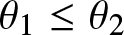
$X\left(\theta_1\right) \; \geq_{lr} \; X\left(\theta_2\right)$, whenever
$\theta_1 \leq \theta_2$;(iii)
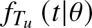
$f_{T_{u}}\left(t| \theta\right)$ is
$TP_2$ in
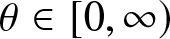
$(t, \theta) \in (0, \infty) \times [0, \infty)$ and is
$RR_2$ in
$(u, \theta) \in (0, \infty) \times [0, \infty)$;(iv)
$T\left(\theta \right) $ is ILR, for all
$\theta \in [0, \infty)$.









Then  ${X}\left(\Theta\right) \; \leq_{lr}\; T_{X} \;\left(\Theta\right)$.
Proof. From (3.14), we get
 \begin{align*}
{f}_{{X_e}\left( \Theta \right)} \left( t\right) = \int_{0}^{\infty} \int_{0}^{\infty} \frac{{f}_T \left( t+u | \theta \right) } {\bar{F}_T \left( u | \theta \right) } f_{X_e}\left( u | \theta \right) g\left( \theta\right)\; du \; d\theta, \quad t \gt 0.
\end{align*}
\begin{align*}
{f}_{{X_e}\left( \Theta \right)} \left( t\right) = \int_{0}^{\infty} \int_{0}^{\infty} \frac{{f}_T \left( t+u | \theta \right) } {\bar{F}_T \left( u | \theta \right) } f_{X_e}\left( u | \theta \right) g\left( \theta\right)\; du \; d\theta, \quad t \gt 0.
\end{align*}Furthermore, from (3.11), we get
 \begin{align*}
{f}_{T_{X}\left( \Theta\right)} \left( t\right) = \int_{0}^{\infty} \int_{0}^{\infty} \frac{{f}_T \left( t+u | \theta \right) } {\bar{F}_T \left( u | \theta \right) } f_{X}\left( u | \theta \right) g\left( \theta\right)\; du \; d\theta, \quad t \gt 0.
\end{align*}
\begin{align*}
{f}_{T_{X}\left( \Theta\right)} \left( t\right) = \int_{0}^{\infty} \int_{0}^{\infty} \frac{{f}_T \left( t+u | \theta \right) } {\bar{F}_T \left( u | \theta \right) } f_{X}\left( u | \theta \right) g\left( \theta\right)\; du \; d\theta, \quad t \gt 0.
\end{align*} Let  $h_1(t , \theta)= \int_{0}^{\infty} \frac{{f}_T \left( t+u | \theta \right) } {\bar{F}_T \left( u | \theta \right) } f_{X_e}\left( u | \theta \right) \; du$ and $h_2(t , \theta)= \int_{0}^{\infty} \frac{{f}_T \left( t+u | \theta \right) } {\bar{F}_T \left( u | \theta \right) } f_{X}\left( u | \theta \right) \; du$, for $t \gt 0$. Now, by using conditions $(i)$ and $(ii)$ in Lemma 2.2, we get that $X\left(\Theta\right) \leq_{lr} X_{e} \left( \Theta \right)$. Thus, to prove the result, it suffices to show that ${X}_{e} \left(\Theta\right) \leq_{lr} T_{X} \;\left(\Theta\right)$, which is equivalent to show that
 \begin{equation}
\frac{\int_{0}^{\infty} h_2\left(t, \theta \right) g\left( \theta\right) \; d\theta } {\int_{0}^{\infty} h_1\left(t , \theta \right) g\left( \theta\right) \; d\theta }\text{is increasing in } t \gt 0.
\end{equation}
\begin{equation}
\frac{\int_{0}^{\infty} h_2\left(t, \theta \right) g\left( \theta\right) \; d\theta } {\int_{0}^{\infty} h_1\left(t , \theta \right) g\left( \theta\right) \; d\theta }\text{is increasing in } t \gt 0.
\end{equation} Now, form condition  $(iv)$, we get $ {{f}_T \left( t+u | \theta \right) }/ {\bar{F}_T \left( u | \theta \right) }$ is $RR_2$ in $(u, t)\in (0,\infty) \times (0,\infty)$. Furthermore, from condition $(iii)$, we get that, for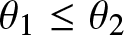 $\theta_1 \leq \theta_2$,
 \begin{equation*}\frac{{f}_T \left( t+u | \theta_1 \right) } {\bar{F}_T \left( u | \theta_1 \right) }\Big/ \frac{{f}_T \left( t+u | \theta_2 \right) } {\bar{F}_T \left( u | \theta_2 \right) }\end{equation*}
is decreasing in  $t \gt 0$ and increasing in $u \gt 0$. Thus, in view of the above two statements along with condition $(ii)$, we get from Lemma 2.1 that
 \begin{equation}
h_2(t , \theta) \text{is } TP_2 \text{in } (t,\theta) \in (0,\infty) \times [0,\infty).
\end{equation}
\begin{equation}
h_2(t , \theta) \text{is } TP_2 \text{in } (t,\theta) \in (0,\infty) \times [0,\infty).
\end{equation} Let  $k(1, u,\theta)= f_{X_e}\left( u| \theta \right)$ and $ k(2, u,\theta) =f_{X}\left( u | \theta \right)$, for $u \gt 0$ and $\theta\geq 0$. From condition $(ii)$, we get that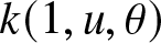 $k(1, u,\theta)$ and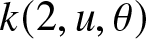 $ k(2, u,\theta)$ are $RR_2$ in $(u, \theta) \in (0, \infty) \times [0, \infty)$. Again, from condition $(i)$, we get that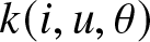 $k(i, u, \theta)$ is $RR_2$ in $(i, u) \in \{1,2\} \times (0, \infty)$ and is $TP_2$ in $(i, \theta) \in \{1,2\} \times [0, \infty)$. Furthermore, from condition $(iii)$, we get that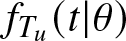 $f_{T_u}(t | \theta)$ is $RR_2$ in $(u, \theta) \in (0, \infty) \times [0, \infty)$. Consequently, by using the above three statements, we get from Theorem 2.2 of Khaledi [Reference Khaledi11] that
 \begin{equation}
\frac{h_2(t,\theta)}{{h_1(t,\theta)}} \text{is increasing in } \theta \geq 0,
\end{equation}
\begin{equation}
\frac{h_2(t,\theta)}{{h_1(t,\theta)}} \text{is increasing in } \theta \geq 0,
\end{equation}for all  $t \gt 0$. Furthermore, by using conditions $(i)$ and $(iv)$, and Theorem 1 $(ii)$ of Hazra et al. [Reference Hazra, Finkelstein and Cha8], we get that
 \begin{equation}
\frac{h_2(t,\theta)}{{h_1(t,\theta)}} \text{is increasing in } t \gt 0,
\end{equation}
\begin{equation}
\frac{h_2(t,\theta)}{{h_1(t,\theta)}} \text{is increasing in } t \gt 0,
\end{equation}for all  $\theta \gt 0$. Finally, by using (3.18), (3.19) and (3.20) in Lemma 2.1, we get (3.17). Hence the result. □
Theorem 3.6 Suppose the following conditions hold true.
(i)
$f_{X_e}(t| \theta)/f_{X}(t|\theta)$ is increasing in
$t \gt 0$ and is decreasing in
$\theta \geq 0$;(ii)
$X\left(\theta_1\right) \; \geq_{lr} \; X\left(\theta_2\right)$, whenever
$\theta_1 \leq \theta_2$;(iii)
$\bar F_{T_{u}}\left(t| \theta\right)$ is
$TP_2$ in
$(t, \theta) \in (0, \infty) \times [0, \infty)$ and is
$RR_2$ in
$(u, \theta) \in (0, \infty) \times [0, \infty)$;(iv)
$T\left(\theta \right) $ is IFR, for all
$\theta \in [0, \infty)$.




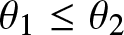
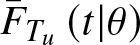





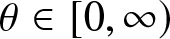
Then  ${X}\left(\Theta\right) \; \leq_{hr}\; T_{X} \;\left(\Theta\right)$. □
Proof. From (3.14), we get
 \begin{align*}
\bar{F}_{{X_e}\left( \Theta \right)} \left( t\right) = \int_{0}^{\infty} \int_{0}^{\infty} \frac{\bar{F}_T \left( t+u | \theta \right) } {\bar{F}_T \left( u | \theta \right) } f_{X_e}\left( u | \theta \right) g\left( \theta\right)\; du \; d\theta, \quad t \gt 0.
\end{align*}
\begin{align*}
\bar{F}_{{X_e}\left( \Theta \right)} \left( t\right) = \int_{0}^{\infty} \int_{0}^{\infty} \frac{\bar{F}_T \left( t+u | \theta \right) } {\bar{F}_T \left( u | \theta \right) } f_{X_e}\left( u | \theta \right) g\left( \theta\right)\; du \; d\theta, \quad t \gt 0.
\end{align*}Furthermore, from (3.11), we get
 \begin{align*}
\bar{F}_{T_{X}\left( \Theta\right)} \left( t\right) = \int_{0}^{\infty} \int_{0}^{\infty} \frac{\bar{F}_T \left( t+u | \theta \right) } {\bar{F}_T \left( u | \theta \right) } f_{X}\left( u | \theta \right) g\left( \theta\right)\; du \; d\theta, \quad t \gt 0.
\end{align*}
\begin{align*}
\bar{F}_{T_{X}\left( \Theta\right)} \left( t\right) = \int_{0}^{\infty} \int_{0}^{\infty} \frac{\bar{F}_T \left( t+u | \theta \right) } {\bar{F}_T \left( u | \theta \right) } f_{X}\left( u | \theta \right) g\left( \theta\right)\; du \; d\theta, \quad t \gt 0.
\end{align*} Let  $h_3(t,\theta)= \int_{0}^{\infty} \frac{\bar{F}_T \left( t+u | \theta \right) } {\bar{F}_T \left( u | \theta \right) } f_{X_e}\left( u | \theta \right) \; du$ and $h_4(t,\theta)= \int_{0}^{\infty} \frac{\bar{F}_T \left( t+u | \theta \right) } {\bar{F}_T \left( u | \theta \right) } f_{X}\left( u | \theta \right) \; du$, for $t \gt 0$. Now, by using conditions $(i)$ and $(ii)$ in Lemma 2.2, we get that $X\left(\Theta\right) \leq_{lr} X_{e} \left( \Theta \right)$. Thus, to prove the result, it suffices to show that ${X}_{e} \left(\Theta\right) \leq_{hr} T_{X} \;\left(\Theta\right)$, which is equivalent to show that
 \begin{equation}
\frac{\int_{0}^{\infty} h_4\left(t, \theta \right) g\left( \theta\right) \; d\theta } {\int_{0}^{\infty} h_3\left(t, \theta \right) g\left( \theta\right) \; d\theta }\text{is increasing in } t \gt 0.
\end{equation}
\begin{equation}
\frac{\int_{0}^{\infty} h_4\left(t, \theta \right) g\left( \theta\right) \; d\theta } {\int_{0}^{\infty} h_3\left(t, \theta \right) g\left( \theta\right) \; d\theta }\text{is increasing in } t \gt 0.
\end{equation} Now, form condition  $(iv)$, we get that $ {\bar{F}_T \left( t+u | \theta \right) }/ {\bar{F}_T \left( u | \theta \right) }$ is $RR_2$ in $(u, t)\in (0,\infty) \times (0,\infty)$. Furthermore, from condition $(iv)$, we get that, for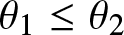 $\theta_1 \leq \theta_2$,
 \begin{equation*}\frac{\bar{F}_T \left( t+u | \theta_1 \right) } {\bar{F}_T \left( u | \theta_1 \right) }\Big/ \frac{\bar{F}_T \left( t+u | \theta_2 \right) } {\bar{F}_T \left( u | \theta_2 \right) }\end{equation*}
is decreasing in  $t \gt 0$ and increasing in $u \gt 0$. Again, from condition $(iv)$, we get that ${\bar{F}_T \left( t+u | \theta_2 \right) } /{\bar{F}_T \left( u | \theta_2 \right) }$ is decreasing in $u \gt 0$. Thus, in view of the above three statements along with the condition “ $X\left(\theta_1\right) \; \geq_{rh} \; X\left(\theta_2\right)$,” we get from Lemma 2.1 that
 \begin{equation}
h_4(t,\theta) \text{is } TP_2 \text{in } (t,\theta) \in (0,\infty) \times [0,\infty).
\end{equation}
\begin{equation}
h_4(t,\theta) \text{is } TP_2 \text{in } (t,\theta) \in (0,\infty) \times [0,\infty).
\end{equation} Let  $k(1, u,\theta) = f_{X_e}\left( u| \theta \right)$ and $ k(2, u,\theta)=f_{X}\left( u | \theta \right)$,for $u \gt 0$ and $\theta\geq 0$. From condition $(ii)$, we get that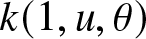 $k(1, u,\theta)$ and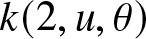 $ k(2, u,\theta)$ are $RR_2$ in $(u,\theta)\in (0, \infty) \times [0, \infty)$. Furthermore, from condition $(i)$, we get that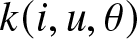 $k(i, u, \theta)$ is $RR_2$ in $(i, u)\in \{1,2\} \times (0, \infty)$ and is $TP_2$ in $(i, \theta) \in \{1,2\} \times [0, \infty)$. Again, from condition $(iii)$, we get that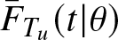 $\bar F_{T_u}(t | \theta)$ is $RR_2$ in $(u , \theta) \in (0, \infty) \times [0, \infty)$. Consequently, from Theorem 2.2 of Khaledi [Reference Khaledi11], we get that
 \begin{equation}
\frac{h_4(t,\theta)}{{h_3(t,\theta)}} \text{is increasing in } \theta \geq 0,
\end{equation}
\begin{equation}
\frac{h_4(t,\theta)}{{h_3(t,\theta)}} \text{is increasing in } \theta \geq 0,
\end{equation}for all  $t \gt 0$. Furthermore, by using conditions $(i)$ and $(iv)$, and Theorem 1 $(iii)$ of Hazra et al. [Reference Hazra, Finkelstein and Cha8], we get that
 \begin{equation}
\frac{h_4(t,\theta)}{{h_2(t,\theta)}} \text{is increasing in } t \gt 0,
\end{equation}
\begin{equation}
\frac{h_4(t,\theta)}{{h_2(t,\theta)}} \text{is increasing in } t \gt 0,
\end{equation}for all  $\theta \gt 0$. Finally, by using (3.22), (3.23) and (3.24) in Lemma 2.1, we get (3.21). Hence the result. □
In the following two theorems, we compare the remaining lifetimes of items drawn from two different populations wherein both have the same generic distribution but different random ages. We study this problem with respect to the usual stochastic order and the likelihood ratio order. The proofs of these theorems follow the same line as the proofs of Theorems 3.5 and 3.6 and are, therefore, omitted.
Theorem 3.7 Suppose the following conditions hold true.
(i)
$X_2\left(\theta\right) \; \leq_{st} (\text{resp. } \geq_{st}) \; X_1\left(\theta\right)$, for all
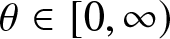
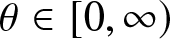
$\theta \in [0, \infty)$;(ii)
$T\left(\theta \right) $ is IFR, for all
$\theta \in [0, \infty)$.


Then  $T_{X_1}\left(\Theta\right) \; \leq_{st} (\text{resp. } \geq_{st}) \; T_{X_2}\left(\Theta\right)$.
Theorem 3.8 Suppose the following conditions hold true.
(i)
$f_{X_1}(t| \theta)/f_{X_2}(t| \theta)$ is increasing in
$t \gt 0$ and is decreasing in
$\theta \geq 0$;(ii) Either
$X_1\left(\theta_1\right) \; \geq_{lr} \; X_1\left(\theta_2\right)$ or
$X_2\left(\theta_1\right) \; \geq_{lr}\; X_2\left(\theta_2\right)$ holds, for
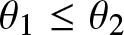
$\theta_1 \leq \theta_2$;(iii)
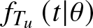
$f_{T_{u}}\left(t| \theta\right)$ is
$TP_2$ in
$(t, \theta) \in (0, \infty) \times [0, \infty)$ and is
$RR_2$ in
$(u, \theta) \in (0, \infty) \times [0, \infty)$;(iv)
$T\left(\theta \right) $ is ILR, for all
$\theta \in [0, \infty)$.










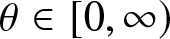
Then  $T_{X_1}\left(\Theta\right) \; \leq_{lr}\; T_{X_2} \;\left(\Theta\right)$. □
If we know how a population’s generic distribution behaves over time, we may use this knowledge to study the ageing properties of the corresponding remaining lifetime of an item. The following simple but practically significant theorem addresses this problem. Its proof is absolutely straightforward and, therefore, for the sake of brevity, is omitted.
Theorem 3.9 The following results are true.
(i) If
$T(\theta)$ is DFR then
$T_{X}(\Theta)$ is DFR;(ii) If
$T(\theta)$ is DLR then
$T_{X}(\Theta)$ is DLR;(iii) If
$T(\theta)$ is IMRL then
$T_{X}(\Theta)$ is IMRL. □


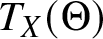

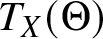
The ageing characteristics of age composition may be useful in certain instances. In the following theorem, we study an ageing property of the random age of an item. Here, we assume that the random lifetime (generic) of an item in a subpopulation does not depend on the calendar time  $t$, i.e., $\bar F_{T_t}(x| \theta) = \bar F (x| \theta)$ and the mixing distribution also does not depend on $t$, i.e., $g_t(\theta ) = g(\theta)$.
Theorem 3.10 Suppose the following conditions hold true.
(i)
$T(\theta_{1}) \leq_{hr} T(\theta_{2})$, for all
$\theta_1 \leq \theta_2$;(ii)
$B_{\theta}\left( t \right) $ is
$RR_2$ in
$(t, \theta) \in [0,u] \times [0, \infty)$ and is log-convex in
$x \in [0, u]$, for all
$\theta \geq 0$;(iii)
$T(\theta)$ is DFR.

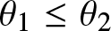



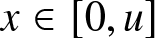


Then 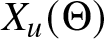 $X_{u}(\Theta)$ is DLR.
Proof. From (3.1), we get
 \begin{align*}
f_{X_u(\Theta)}(t)= \int_{0}^{\infty} \frac{B_{\theta}\left( u-t \right)\bar{F}\left( t | \theta\right) }{\int_{0}^{u}B_{\theta}\left( u-w \right)\bar{F}\left( w | \theta\right)\;dw } g(\theta) \; d\theta , \quad 0\leq t \leq u .
\end{align*}
\begin{align*}
f_{X_u(\Theta)}(t)= \int_{0}^{\infty} \frac{B_{\theta}\left( u-t \right)\bar{F}\left( t | \theta\right) }{\int_{0}^{u}B_{\theta}\left( u-w \right)\bar{F}\left( w | \theta\right)\;dw } g(\theta) \; d\theta , \quad 0\leq t \leq u .
\end{align*}Thus, to prove the result, it suffices to show that
 \begin{equation}
\frac{f_{X_u(\Theta)}(t+a) }{f_{X_u(\Theta)}(a) } \text{is increasing in } a\in [0,u].
\end{equation}
\begin{equation}
\frac{f_{X_u(\Theta)}(t+a) }{f_{X_u(\Theta)}(a) } \text{is increasing in } a\in [0,u].
\end{equation} Now, from condition “ $T(\theta_{1}) \leq_{hr} T(\theta_{2})$, for all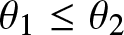 $\theta_1 \leq \theta_2$,” we get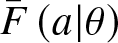 $\bar{F}\left( a | \theta\right)$ is $TP_2$ in $(a , \theta) \in [0,u] \times [0,\infty)$, and from condition “ $B_{\theta}\left( t \right) $ is $RR_2$ in $(t, \theta) \in [0,u] \times [0, \infty)$,” we get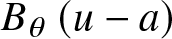 $B_{\theta}\left( u-a \right) $ is $TP_2$ in $(a, \theta) \in [0,u] \times [0, \infty)$. Again, these two conditions together imply that
 \begin{equation}
\frac{B_{\theta}\left( u-a \right)\bar{F}\left( a | \theta\right) }{\int_{0}^{u}B_{\theta}\left( u-w \right)\bar{F}\left( w | \theta\right)\;dw } \text{is } TP_2 \text{in } (a, \theta) \in [0,u] \times [0, \infty),
\end{equation}
\begin{equation}
\frac{B_{\theta}\left( u-a \right)\bar{F}\left( a | \theta\right) }{\int_{0}^{u}B_{\theta}\left( u-w \right)\bar{F}\left( w | \theta\right)\;dw } \text{is } TP_2 \text{in } (a, \theta) \in [0,u] \times [0, \infty),
\end{equation}which further implies that
 \begin{equation}
\frac{\frac{B_{\theta}\left( u-t-a \right)\bar{F}\left( t+a | \theta\right) }{\int_{0}^{u}B_{\theta}\left( u-w \right)\bar{F}\left( w | \theta\right)\;dw } } {\frac{B_{\theta}\left( u-a \right)\bar{F}\left( a | \theta\right) }{\int_{0}^{u}B_{\theta}\left( u-w \right)\bar{F}\left( w | \theta\right)\;dw } } \text{is increasing in } \theta \in [0, \infty).
\end{equation}
\begin{equation}
\frac{\frac{B_{\theta}\left( u-t-a \right)\bar{F}\left( t+a | \theta\right) }{\int_{0}^{u}B_{\theta}\left( u-w \right)\bar{F}\left( w | \theta\right)\;dw } } {\frac{B_{\theta}\left( u-a \right)\bar{F}\left( a | \theta\right) }{\int_{0}^{u}B_{\theta}\left( u-w \right)\bar{F}\left( w | \theta\right)\;dw } } \text{is increasing in } \theta \in [0, \infty).
\end{equation} By using conditions “ $B_{\theta}\left( t \right) $ is log-convex in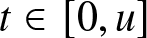 $t \in [0, u]$, for all $\theta \geq 0$” and “ $T(\theta)$ is DFR” in Theorem 8 of Hazra et al. [Reference Hazra, Finkelstein and Cha8], we get that
 \begin{equation}
\frac{\frac{B_{\theta}\left( u-t-a \right)\bar{F}\left( t+a | \theta\right) }{\int_{0}^{u}B_{\theta}\left( u-w \right)\bar{F}\left( w | \theta\right)\;dw } } {\frac{B_{\theta}\left( u-a \right)\bar{F}\left( a | \theta\right) }{\int_{0}^{u}B_{\theta}\left( u-w \right)\bar{F}\left( w | \theta\right)\;dw } } \text{is increasing in } a \in [0, u].
\end{equation}
\begin{equation}
\frac{\frac{B_{\theta}\left( u-t-a \right)\bar{F}\left( t+a | \theta\right) }{\int_{0}^{u}B_{\theta}\left( u-w \right)\bar{F}\left( w | \theta\right)\;dw } } {\frac{B_{\theta}\left( u-a \right)\bar{F}\left( a | \theta\right) }{\int_{0}^{u}B_{\theta}\left( u-w \right)\bar{F}\left( w | \theta\right)\;dw } } \text{is increasing in } a \in [0, u].
\end{equation}Finally, by using (3.26), (3.27) and (3.28) in Lemma 2.2, we get (3.25). Hence, the result is proved. □
In the following example, we demonstrate the result given in Theorem 3.4.
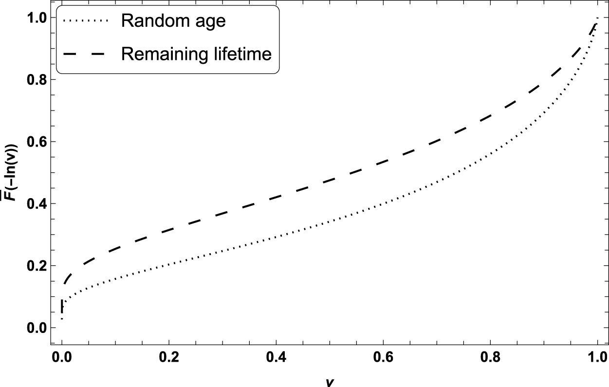
Example 3.2. Consider an item with random age  $X\left(\Theta\right)$ and remaining lifetime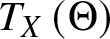 $T_X\left(\Theta\right)$, where $\bar F_X(t, \theta) = e^{-\alpha \theta t}$, $\bar F_T(t, \theta) = e^{-\beta \theta t}$, $t \gt 0$,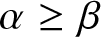 $\alpha \geq \beta$, and $g(\theta) = 1/(1+ \theta)^2$, $\theta \gt 0$. It can be easily verified that all conditions of Theorem 3.4 are satisfied. Furthermore, by plotting $\bar F_{T_X\left(\Theta\right)}(-\ln(v))$ and $\bar F_{X\left(\Theta\right)}(-\ln(v)) $, against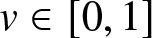 $ v\in[0,1]$ in Figure 2, it shows that $\bar F_{X\left(\Theta\right)}(-\ln(v)) \leq \bar F_{T_X\left(\Theta\right)}(-\ln(v)) $, for all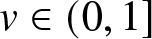 $v\in(0,1]$ and so, $\bar F_{X\left(\Theta\right)}(t) \leq \bar F_{T_X\left(\Theta\right)}(t) $, for all $t \gt 0$. Thus, $X\left(\Theta\right) \leq_{st}\; T_X\left(\Theta\right)$. □
Plot of  $\bar F_{T_X\left(\Theta\right)}(-\ln(v))$ and $\bar F_{X\left(\Theta\right)}(-\ln(v)) $ against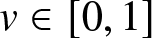 $ v\in[0,1]$.

4. Concluding remarks
In understanding the lifetime behavior of a population of manufactured items, it is important to know how the initial age of an item impacts on its remaining lifetime. In practice, items are generally produced in bulk and stored in warehouses prior to sale. In many cases, it is not known when an item is sold or when it is incepted into operation. Thus, it is natural to assume that an item drawn at random from a population has some initial age at the time of inception. Moreover, this initial age is most often unknown and consequently, it can be considered as a random quantity, which we formally call the random initial age.
Another “origin” of a random age (age composition) considered in detail in our paper is when it naturally arises in the populations of continuously manufactured and incepted into operation items. In particular, we consider populations of heterogeneous items having random initial age. We discuss two different age compositions for this population and study some stochastic comparisons. We compare the random ages of items drawn from heterogeneous populations under different modeling frameworks. Specifically, we consider populations generated by mixing age compositions of subpopulations (Model I) and populations generated by mixing at the level of an individual item (Model II), as well as direct comparisons between populations arising from Models I and II. Throughout the analysis, we assume that the generic lifetime distribution of items in each subpopulation does not depend on the calendar time, that is,  $\bar F_{T_t}(x, \theta)= \bar F(x, \theta)$, and that the mixing distribution is time-independent, $g_t(\theta)=g(\theta)$. We also derive the distribution of the remaining lifetime and analyze its “connection” with the random initial age and the associated equilibrium distribution. In particular, we show that when the random age distribution in each subpopulation coincides with the corresponding equilibrium distribution, the random age and the remaining lifetime of an item in a heterogeneous population are stochastically identical. This naturally leads to the question of identifying conditions under which the remaining lifetime is stochastically larger or smaller than the random age. This question is addressed through several stochastic ordering results derived in the subsequent theorems. We further compare the remaining lifetimes of items drawn from two different heterogeneous populations that share the same generic lifetime distribution but differ in their random age distributions, and establish comparisons with respect to different stochastic orders. Furthermore, we investigate ageing properties of both the remaining lifetime and the random age, showing how knowledge of the generic lifetime distribution can be used to infer ageing behavior in heterogeneous populations.
The obtained comparisons are relevant for practical situations involving large volume of manufactured items, where heterogeneity naturally arises due to variability in production quality or operating conditions. The stochastic ordering results can be used to assess and compare the ageing properties and reliability of different populations, supporting decisions related to replacement and maintenance policies. In particular, they can be used to assess the ageing of a population of items in use; for example, a stochastically larger random age indicates a higher proportion of older items, which may indicate the need for increased inspection, preventive maintenance, or timely replacement. Conversely, a stochastically smaller age distribution may reflect a relatively “younger” and more reliable population, requiring less intensive maintenance planning. In addition, the ageing properties derived for random age and remaining lifetime provide insight into how population heterogeneity affects long-term system performance. In practice, the age composition of an item and its remaining lifetime (in homogeneous and heterogeneous populations) can be dependent, whereas all studies including the current one assume independence. This challenging topic is yet to be investigated. We are currently working on this problem and will hopefully report the outputs in future communications.
Acknowledgements
The authors would like to thank the Editor-in-Chief, the Associate Editor and the anonymous reviewers for their valuable constructive comments/suggestions, which have led to an improved version of the manuscript.
The first author sincerely acknowledges the financial support received from IIT Palakkad, India. The work of the second author was supported by IIT Jodhpur, India.




 Open access

