


1. Introduction
Thermo-responsive hydrogels are polymers whose degree of swelling depends on the ambient temperature. Hydrogels absorb and retain significant amounts of fluid, resulting in swelling of the solid structure as the fluid fills the interstitial space between polymer chains (see figure 1). This swelling can be substantial, with the volume of some hydrogels increasing several fold compared to their dry form (Tanaka Reference Tanaka1978; Hirokawa & Tanaka Reference Hirokawa and Tanaka1984). Thermo-responsive hydrogels have a sharp decrease in their affinity for the fluid when heated above a certain temperature, called the volume phase transition temperature, resulting in expulsion of much of the interstitial fluid and significant shrinking of the gel. Many other responsive gels have also been developed in recent years, with a variety of different controlling external stimuli, such as pH, electric charge and light (Koetting et al. Reference Koetting, Peters, Steichen and Peppas2015; Erol et al. Reference Erol, Pantula, Liu and Gracias2019). However, responsive hydrogels actuated by temperature are of particular interest, especially gels such as poly(N-isopropylacrylamide) – or PNIPAM – because they have a sharp transition in their degree of swelling at temperatures that are easily obtainable experimentally, and often biomedically relevant (Haq, Su & Wang Reference Haq, Su and Wang2017).
(a) A scanning electron microscope (SEM) image of the micro-structure of PNIPAM, reprinted from Ju et al. (Reference Ju, Chu, Zhu, Hu, Song and Chen2006) with permission from IOP Publishing. (b) Schematic of a thermo-responsive hydrogel's structure – as the gel is heated, it loses its affinity for the fluid in the pore space, hence it contracts and expels fluid.

Developing materials that change size in a controllable way gives a route to creating controllable shape change. For example, having two (or more) materials joined together that swell or shrink differently under a given stimulus can generate internal elastic stresses that are relaxed by deforming; differential swelling can cause out-of-plane buckling, and careful choice of the material properties and geometry during fabrication can allow for a whole host of possible programmed transformations (Holmes Reference Holmes2019). Hydrogels with controllable swelling are therefore a promising avenue for developing shape-changing devices. This is particularly true at small scales, where recent technological advances allow for micro-scale design and manufacture of gel structures through techniques such as three-dimensional printing via two-photon polymerisation, otherwise known as 2PP (Hippler et al. Reference Hippler, Blasco, Qu, Tanaka, Barner-Kowollik, Wegener and Bastmeyer2019; Ji et al. Reference Ji, Luan, Yao, Fu and He2021), and halftone gel or stop flow lithography (Kim et al. Reference Kim, Hanna, Byun, Santangelo and Hayward2012; Sharan et al. Reference Sharan, Maslen, Altunkeyik, Rehor, Simmchen and Montenegro-Johnson2021). Such small devices have a wide range of physical applications (Ionov Reference Ionov2014), for example as microfluidic valves (Harmon, Tang & Frank Reference Harmon, Tang and Frank2003; Richter et al. Reference Richter, Kuckling, Howitz, Gehring and Arndt2003), as grippers that could be used by soft robots (Li et al. Reference Li, Cai, Gao and Serpe2017), and as actuation for swimming in microbots or artificial active matter (Masoud, Bingham & Alexeev Reference Masoud, Bingham and Alexeev2012; Nikolov, Yeh & Alexeev Reference Nikolov, Yeh and Alexeev2015; Mourran et al. Reference Mourran, Zhang, Vinokur and Möller2017; Montenegro-Johnson Reference Montenegro-Johnson2018; Wischnewski & Kierfeld Reference Wischnewski and Kierfeld2020).
There are many opportunities to exploit stimuli-responsive hydrogels in biomedical settings (Klouda Reference Klouda2015; Sood et al. Reference Sood, Bhardwaj, Mehta and Mehta2016). Controllable delivery of small quantities of drugs to a specific site could improve patient outcomes by reducing the required dosage necessary for a treatment; such dosing cannot be addressed by conventional drug delivery methods (Li & Mooney Reference Li and Mooney2016). Responsive hydrogels are an appropriate and flexible means to achieve this targeted drug delivery (Peppas Reference Peppas1997; Qiu & Park Reference Qiu and Park2001; Schmaljohann Reference Schmaljohann2006; Qureshi et al. Reference Qureshi, Nayak, Maji, Anis, Kim and Pal2019; Marques et al. Reference Marques, Costa, Velho and Amaral2021). The drug can be either embedded within the microstructure of the gel itself and released as it contracts (Kulkarni & Biswanath Reference Kulkarni and Biswanath2007; Bhattarai, Gunn & Zhang Reference Bhattarai, Gunn and Zhang2010), or encapsulated within a microscopic delivery device that opens when actuated (Stoychev, Puretskiy & Ionov Reference Stoychev, Puretskiy and Ionov2011; Fan et al. Reference Fan, Chung, Lim, Li and Loh2016), with the stimuli either externally imposed or dependent on the immediate environment. Additional control over the drug release can be obtained by combining multiple stimuli (Fu et al. Reference Fu, Hosta-Rigau, Chandrawati and Cui2018) or through timed actuation, allowing multiple-dose strategies to be developed. Responsive hydrogels also have applicability in other medically relevant scenarios, for example being used as scaffolds in tissue engineering, as an aid for wound healing, and as components in microtools for use in microsurgery (Sood et al. Reference Sood, Bhardwaj, Mehta and Mehta2016; Erol et al. Reference Erol, Pantula, Liu and Gracias2019).
To fully understand the shape-changing properties of responsive hydrogel devices, a key first step is to understand how the size change occurs in a simple homogeneous gel. In particular, the dynamics of the swelling or shrinking of such a gel will be an important component in determining how a more complicated material behaves during the swelling and shrinking process. Experiments on these thermo-responsive gels have suggested that there is a difference between the behaviour of a homogeneous gel when swelling, compared to when shrinking: dynamic swelling has been observed to equilibrate exponentially, whereas the dynamics of a shrinking gel appears more complicated and can exhibit an instability that forms lobe-like structures (Sato Matsuo & Tanaka Reference Sato Matsuo and Tanaka1988). Temperature changes beyond transition have been observed to cause separation into distinct swollen and shrunken states along the length of a cylinder, with an appearance similar to the fluid-dynamical Rayleigh–Plateau instability (Matsuo & Tanaka Reference Matsuo and Tanaka1992), as well as through the appearance of surface blisters that can cause deformation of rods and tori (Chang et al. Reference Chang, Dimitriyev, Souslov, Nikolov, Marquez, Alexeev, Goldbart and Fernández-Nieves2018; Shen et al. Reference Shen, Kan, Benet and Vernerey2019).
Since the size change of hydrogels is dependent on the movement of fluid into or out of the polymer structure, the dynamics of swelling and shrinking are fundamentally problems of fluid dynamics, coupled with solid mechanics and polymer physics. Some of the earliest approaches to modelling such systems focused on the diffusion of the cross-linked polymer network, whilst ignoring the fluid motion (Tanaka, Hocker & Benedek Reference Tanaka, Hocker and Benedek1973; Tanaka & Fillmore Reference Tanaka and Fillmore1979). More recent work has incorporated all three physical building blocks into continuum mechanical models of hydrogels (e.g. Hong et al. Reference Hong, Zhao, Zhou and Suo2008; Doi Reference Doi2009; Chester & Anand Reference Chester and Anand2011; Engelsberg & Barros Reference Engelsberg and Barros2013; Bertrand et al. Reference Bertrand, Peixinho, Mukhopadhyay and MacMinn2016; Drozdov & Christiansen Reference Drozdov and Christiansen2017). These models are typically poro-elastic, and are constructed via a model for the free energy density of swelling, based on Flory–Rehner theory (Flory & Rehner Reference Flory and Rehner1943a,Reference Flory and Rehnerb), that has three main components: mixing of the fluid and polymer, deformation of the polymer structure, and work against the chemical potential or fluid pressure. The hydrogel can undergo large deformations when swelling and shrinking, so the material is often taken to be hyperelastic, for example using a neo-Hookean energy density. The fluid motion within the hydrogel mixture is then modelled diffusively (Hong et al. Reference Hong, Zhao, Zhou and Suo2008; Engelsberg & Barros Reference Engelsberg and Barros2013) or using Darcy flow (Doi Reference Doi2009; Bertrand et al. Reference Bertrand, Peixinho, Mukhopadhyay and MacMinn2016).
These models have been applied to a range of scenarios involving generic hydrogels, including the evolution of gel filters (Doi Reference Doi2009) and gel systems under load (Hong et al. Reference Hong, Zhao, Zhou and Suo2008), and as a model system for plant transpiration (Etzold, Linden & Worster Reference Etzold, Linden and Worster2021). Finite element simulations have been used to investigate the large deformation behaviour of swelling hydrogels (Lucantonio, Nardinocchi & Teresi Reference Lucantonio, Nardinocchi and Teresi2013). Other studies modelling hydrogel spheres have also uncovered complex internal dynamics when swelling and shrinking, such as core–shell behaviour and transient surface instabilities (Bertrand et al. Reference Bertrand, Peixinho, Mukhopadhyay and MacMinn2016; Curatolo et al. Reference Curatolo, Nardinocchi, Puntel and Teresi2017). In addition, theoretical modelling of one-dimensional hydrogels has isolated the physics of the swelling from the geometry, from which it is possible to investigate when and how phase separation into states with different degrees of swelling occurs (Hennessy, Münch & Wagner Reference Hennessy, Münch and Wagner2020).
These theoretical models have also been applied specifically to thermo-responsive hydrogels. Diffusive models of swelling and shrinking thermo-responsive gels suggest that the time scale for swelling or shrinking scales with the square of the gel size, agreeing with experimental observations (Tanaka et al. Reference Tanaka, Sato, Hirokawa, Hirotsu and Peetermans1985), and have been used to predict the dynamic swelling of spherical shells (Wahrmund et al. Reference Wahrmund, Kim, Chu, Wang, Li, Fernandez-Nieves, Weitz, Krokhin and Hu2009). Following predictions for the phase separation of thermo-responsive hydrogels based on their free energy density (Sekimoto Reference Sekimoto1993), the dynamics of a one-dimensional hydrogel bar with regions of different swelling was explored using a mechanical model that balances internal hydrogel stresses with friction between polymer and fluid within the gel (Tomari & Doi Reference Tomari and Doi1994). This modelling approach was developed further to investigate the dynamics of spherical thermo-responsive hydrogels close to the transition temperature (Tomari & Doi Reference Tomari and Doi1995). This work reproduced theoretically the experimental observations of two-stage swelling and shrinking dynamics, and predicted the occurrence of transient phase separation into concentric swollen and collapsed states close to the volume phase transition, similar to the previously mentioned core–shell behaviour observed in other hydrogel systems, which has since been enforced by other studies (Doi Reference Doi2009). In recent years, several studies have focused on applying large deformation mechanics to thermo-responsive hydrogel problems, which has resulted in finite element simulations for the swelling of cubes, discs and more complex geometries (Chester & Anand Reference Chester and Anand2011; Drozdov & Christiansen Reference Drozdov and Christiansen2017). These methods are excellent for specific applications; however, there is still room for more fundamental studies of the generic swelling behaviour of hydrogels in simplified systems.
In this work, we apply the poro-elastic model of Bertrand et al. (Reference Bertrand, Peixinho, Mukhopadhyay and MacMinn2016) – which was used to study the swelling of a dry spherical gel bead immersed in water and the subsequent drying by evaporation – to investigate the dynamic swelling and shrinking of a thermo-responsive hydrogel sphere in a quiescent fluid bath. In particular, we consider the evolution of a thermo-responsive hydrogel sphere after a sudden temperature change for two different model systems that have been observed experimentally, and consider their behaviour during both swelling and shrinking. The temperature change is taken as instantaneous since diffusion of heat occurs much faster than hydrogel swelling. We aim to extend the work of Tomari & Doi (Reference Tomari and Doi1995) in a few key ways. First, we note that Tomari & Doi (Reference Tomari and Doi1995) focused on the dynamics for temperatures close to the transition between swollen and shrunken states, whereas we will consider characterising the behaviours for more significant temperature changes. In addition, we use a fully poro-elastic model that includes explicitly the fluid flow within the mixture, which Tomari & Doi (Reference Tomari and Doi1995) account for using a viscous dissipation term. This additional component makes an important contribution to the physics of the system, which can result in a significant difference to resultant behaviours (Hui & Muralidharan Reference Hui and Muralidharan2005). Moreover, we will investigate an approximate analytic solution that encapsulates the key physics of the core–shell shrinking dynamics, which is simple enough to be used in applications such as designing drug-dosing strategies. We will comment on any similarities and differences between our results and those of Tomari & Doi (Reference Tomari and Doi1995) as they arise.
We begin in § 2 by introducing the equilibrium model for the thermo-responsive hydrogel, before outlining the dynamic model in § 3. The poro-elastic equations for the evolution of the hydrogel sphere are then solved numerically, with example results for swelling and shrinking of each of the two model systems presented in § 4. We observe a range of different behaviours in the swelling and shrinking dynamics in both cases, such as swelling occurring smoothly inwards from the edge upon cooling, but reheating resulting in a sharp front between a swollen core and shrunken shell (see schematic in figure 2). Other distinct behaviours are also seen, and we provide an overview of when each is expected to occur. The dynamics of the shrinking gel is often characterised by an inwards-travelling front, which we investigate further in § 5 using an approximate analytic solution. We show that this solution can be evolved forwards in time, and investigate a potential application in calculating drug-dosage strategies. Finally, we summarise our results in § 6.
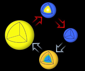
A thermo-responsive hydrogel sphere shrinks as it is heated and swells as it is cooled. Colour denotes porosity (or degree of swelling). Swelling occurs smoothly from the edge, whereas for shrinking, a sharp inwards-propagating front is formed between two (nearly) uniform porosity regions. These illustrations are results from our study (see figures 5 and 6), presented here to orient the reader with the discussions that follow.

2. Equilibrium swelling of a hydrogel
2.1. Free energy density of the hydrogel
We consider a hydrogel in a quiescent bath of fluid that has absorbed fluid and deformed. Both of these processes have energy costs associated with them: a chemical contribution from the mixing of fluid molecules and polymer chains, and a physical contribution from the elastic deformation of the polymer. The nominal free energy density of the hydrogel in such a state can then be written as the sum of these two contributions (Flory & Rehner Reference Flory and Rehner1943a,Reference Flory and Rehnerb)
 \begin{equation} \tilde{W} = \tilde{W}_{{elast}} + \tilde{W}_{{mix}}, \end{equation}
where  $\tilde {W}_{{elast}}$ represents the elastic energy density and $\tilde {W}_{{mix}}$ is the mixing energy density. Here, $\tilde {W}$ is the Helmholtz free energy of the mixture per unit volume of the undeformed dry polymer. Throughout this work, we use tildes, $\tilde {\cdot }$, to denote dimensional quantities.
We consider a gel deformation from a reference state, resulting in a local factor increase in volume of the body,  $J$, relative to this reference state (at which $J=1$). The principal stretches $\lambda _i$ for $i\in \{1,2,3\}$ are the factor increase in lengths from the reference state in each direction; they are the major and minor axes of an ellipsoid that results from the deformation (locally) of a unit sphere in the reference state. The local volume change $J$ is therefore the product of the stretches, $J=\lambda _1\lambda _2\lambda _3$.
Such a deformation has an energetic cost to stretching (or compressing) the polymer chains. We consider a neo-Hookean model for the elastic energy density:
 \begin{equation} \tilde{W}_{{elast}} = \frac{\tilde{G}}{2} \left[ \lambda_1^2 + \lambda_2^2 + \lambda_3^2 - 3 - 2 \log J \right], \end{equation}
where  $\tilde {G}$ is the shear modulus of the gel. Commonly, the shear modulus is found to follow a linear behaviour with temperature, $\tilde {G}=\tilde {k}_B\tilde {T}/\tilde {\varOmega }_p$, where $\tilde {T}$ is the temperature (in kelvin), $\tilde {k}_B$ is the Boltzmann constant, and $\tilde {\varOmega }_p$ is the volume of polymer per polymer molecule in the reference state. (Note that often this is written as $\tilde {G}=\tilde {N}\tilde {k}_B\tilde {T}$, with $\tilde {N}$ the number density of polymer chains in the reference state, but $\tilde {N}$ and $\tilde {\varOmega }_p$ are related simply through $\tilde {N}=1/\tilde {\varOmega }_p$.)
For the mixing contribution to the free energy density, we use the Flory–Huggins polymer theory (Flory Reference Flory1942; Huggins Reference Huggins1942; Flory & Rehner Reference Flory and Rehner1943b) to get the mixing energy density
 \begin{equation} \tilde{W}_{{mix}}= \frac{\tilde{k}_B \tilde{T}}{\tilde{\varOmega}_f}\,J \left[ \phi\log\phi + \chi\phi(1-\phi) \right]. \end{equation}
Here,  $\phi$ is the porosity (i.e. the local proportion of fluid per unit mixture volume), and $\tilde {\varOmega }_f$ is the volume of fluid per fluid molecule in the unmixed state. Note that in (2.3), there is a factor $J$ to account for the local volume change relative to the reference state, due to deformation of the gel.
The term  $\chi$ in (2.3) is the (Flory) mixing parameter, and gives the degree to which the polymer and fluid like to mix; in general, this mixing parameter can depend on both temperature and mixture composition, $\chi = \chi (\tilde {T},\phi )$. It has been suggested that both components are required to reproduce experimental data accurately (Lopez-Leon & Fernandez-Nieves Reference Lopez-Leon and Fernandez-Nieves2007). There are many possible options for this function, but for simplicity, we focus on a relationship that is linear in both the temperature and the polymer fraction:
 \begin{equation}
\left.\begin{gathered} \chi(\tilde{T},\phi) =
\chi_0(\tilde{T}) + \chi_1(\tilde{T})\,(1-\phi), \\
\chi_0(\tilde{T})= A_0 + B_0 \tilde{T},\quad
\chi_1(\tilde{T}) = A_1 + B_1 \tilde{T},
\end{gathered}\right\}
\end{equation}
\begin{equation}
\left.\begin{gathered} \chi(\tilde{T},\phi) =
\chi_0(\tilde{T}) + \chi_1(\tilde{T})\,(1-\phi), \\
\chi_0(\tilde{T})= A_0 + B_0 \tilde{T},\quad
\chi_1(\tilde{T}) = A_1 + B_1 \tilde{T},
\end{gathered}\right\}
\end{equation}
where  $A,B$ are constants, as modelled by Cai & Suo (Reference Cai and Suo2011). We note, however, that many other models for this mixing parameter exist: constant (Hong et al. Reference Hong, Zhao, Zhou and Suo2008; Bertrand et al. Reference Bertrand, Peixinho, Mukhopadhyay and MacMinn2016; Hennessy et al. Reference Hennessy, Münch and Wagner2020), dependent only on the temperature (Tomari & Doi Reference Tomari and Doi1995; Chester & Anand Reference Chester and Anand2011), or with more complicated behaviours, such as including terms inversely proportional to temperature (Tanaka Reference Tanaka1978; Quesada-Pérez et al. Reference Quesada-Pérez, Maroto-Centeno, Forcada and Hidalgo-Alvarez2011) or quadratic powers (Drozdov & Christiansen Reference Drozdov and Christiansen2017). We have chosen to use the linear relation (2.4) because it is simple, yet still includes the important local composition dependence. Despite this simplicity, different choices of the constants can give a range of different behaviours, both quantitatively and qualitatively.
To relate the polymer fraction and  $J$, we must define the reference state, where $J=1$ everywhere. For simplicity, and in line with many other works on hydrogel swelling (Doi Reference Doi2009; Bertrand et al. Reference Bertrand, Peixinho, Mukhopadhyay and MacMinn2016; Hennessy et al. Reference Hennessy, Münch and Wagner2020), we consider the reference state to be the dry state, where the polymer is a solid block with $\phi =0$; we note, however, that there is some debate as to what an appropriate reference state is, and whether such a completely dry state is indeed physical (Quesada-Pérez et al. Reference Quesada-Pérez, Maroto-Centeno, Forcada and Hidalgo-Alvarez2011). Treating the polymer chains as incompressible and the mixture as ideal, the relation between the volume change and solid fraction is then given simply by
 \begin{equation} J=\frac{1}{1-\phi}. \end{equation}
2.2. Free-swelling equilibria
We now turn to consider the equilibrium swelling of a hydrogel. Under free-swelling conditions, where no external stresses are applied to the hydrogel, and the background fluid in the surrounding environment is static, the stretches in each direction must be equal,  $\lambda _i=\lambda$ with $J=\lambda ^3$. The free energy density can therefore be rewritten as a function of $\lambda$ only:
 \begin{align} \tilde{W}(\lambda) = \frac{3\tilde{G}}{2} \left[ \lambda^2 - 1 - 2 \log \lambda \right] + \frac{\tilde{k}_B \tilde{T}}{\tilde{\varOmega}_f} \left[ (\lambda^3-1)\log\left(1-\frac{1}{\lambda^3}\right) + \chi\left(1-\frac{1}{\lambda^3}\right) \right], \end{align}
with  $\chi =\chi _0(\tilde {T}) + \chi _1(\tilde {T})/\lambda ^3$.
Equilibria are found by minimising the free energy density so that  $\mathrm {d} \tilde {W}(\lambda )/\mathrm {d} \lambda =0$; the equilibrium stretch $\lambda$ must therefore satisfy the equation
 \begin{equation} \frac{\lambda^2 - 1}{\lambda^3} + \varOmega \left[ \log\left(1-\frac{1}{\lambda^3}\right) + \frac{1}{\lambda^3} + \frac{\chi_0-\chi_1}{\lambda^6} + \frac{2\chi_1}{\lambda^9} \right] = 0. \end{equation}
Given the mixing parameter  $\chi (\tilde {T},\phi )$, the equilibrium solutions $\lambda =\lambda (\tilde {T};\varOmega )$ can then be calculated as a function of temperature with a single parameter, $\varOmega = \tilde {\varOmega }_p/\tilde {\varOmega }_f$. This parameter encodes the relative importance of the mixing and elastic energies, but it is also the ratio of volume per polymer chain compared to a fluid molecule (or, alternatively, a ratio of their densities) and is in general expected to be large. The value of this parameter may vary depending on factors such as the gel composition and curing conditions (since these affect the stiffness of the gel), and can take values from tens (Quesada-Pérez et al. Reference Quesada-Pérez, Maroto-Centeno, Forcada and Hidalgo-Alvarez2011; Drozdov Reference Drozdov2014) to hundreds (Tanaka Reference Tanaka1978; Cai & Suo Reference Cai and Suo2011) and above (Bertrand et al. Reference Bertrand, Peixinho, Mukhopadhyay and MacMinn2016).
To complete the calculation of the equilibrium swelling, it therefore remains to define the functions  $\chi _0$ and $\chi _1$, i.e. choose values for the constants $A$ and $B$ in (2.4). Even after restricting the equilibrium swelling to certain qualitative behaviour (such as being more swollen at low temperatures, with a swelling transition within a certain temperature range), there remains a wide range of possible choices for these parameters; we consider two possibilities using equilibrium data extracted from the literature.
In the first case, we take the values used previously by Cai & Suo (Reference Cai and Suo2011) in modelling the mechanics of a thermo-responsive hydrogel:
 \begin{equation} \left.\begin{gathered} \varOmega = 100, \\ A_0 ={-}12.947,\quad A_1 = 17.92, \\ B_0 = 0.04496\,\text{K}^{{-}1},\quad B_1 ={-}0.0569\,\text{K}^{{-}1}. \end{gathered}\right\} \end{equation}
The values of  $A$ and $B$ given here were determined by Afroze, Nies & Berghmans (Reference Afroze, Nies and Berghmans2000) from a prepared sample of PNIPAM. In this case, the equilibrium curve is multi-valued, taking a characteristic S-shape as shown in figure 3(a). We will refer to this as the Afroze–Nies–Berghmans (ANB) solution. Small changes in temperature can result in a large (discontinuous) jump in the level of equilibrium swelling. This equilibrium behaviour has been observed experimentally in some thermo-responsive hydrogels (e.g. Tanaka Reference Tanaka1978; Hirokawa & Tanaka Reference Hirokawa and Tanaka1984; Sato Matsuo & Tanaka Reference Sato Matsuo and Tanaka1988). The volume phase transition temperature for shrinking in this example is $\tilde {T}_c\approx 305.8$ K, and we expect a large degree of shrinking when the temperature is increased above this. However, we note that there is a small range of temperatures over which there are multiple possible equilibrium solutions (the system exhibits hysteresis); when decreasing the temperature from an originally deswollen state, the hydrogel will swell significantly only once below the volume phase transition for swelling, $\tilde {T}_c\approx 304.7$ K, which is lower than that for the shrinking transition.
Equilibrium swelling of thermo-responsive hydrogels under free-swelling conditions (solid curves) for (a) the ANB parameters (2.8), and (b) the HHT parameters (2.9). The stretch (or factor increase in lengths compared to the dry state)  $\lambda$ is calculated as a function of temperature $\tilde {T}$ using (2.7). The dashed lines show the spinodal curves, where $\partial ^2 \tilde {W}/\partial \lambda _i^2=0$, with the spinodal regions being the darker shaded areas, $\partial ^2 \tilde {W}/\partial \lambda _i^2<0$. The lighter shaded regions are where the isotropically-stretched state can coexist alongside another with a discontinuous normal stretch across the interface. In (b), the fitted curve is compared to (rescaled) data from Hirotsu et al. (Reference Hirotsu, Hirokawa and Tanaka1987), and the inset shows a zoom of the region close to the swelling transition.

We also consider an example that is found by fitting (2.7) to data captured from figure 3 of Hirotsu, Hirokawa & Tanaka (Reference Hirotsu, Hirokawa and Tanaka1987) for another sample of PNIPAM. To do this, we rearrange (2.7) to  $\tilde {T}=\tilde {T}(\lambda )$, and fit the appropriate six parameters, which are $\varOmega,A_0,B_0,A_1,B_1$ and the scaling between their gel radius and the stretch (i.e. determine the radius at which $\lambda =1$, since this is unknown in the experiment). This fitting was implemented using the MATLAB least-squares fitting nonlinlsq from the Optimization Toolbox, running the fitting a large number of times to remove any local minima that were found. The best-fit parameters are found to be
 \begin{equation} \left.\begin{gathered} \varOmega = 720, \\ A_0 ={-}62.22,\quad A_1 ={-}58.28, \\ B_0 = 0.20470\,\text{K}^{{-}1},\quad B_1 = 0.19044\,\text{K}^{{-}1}, \end{gathered}\right\} \end{equation}
with the scaling between the data and the equilibrium stretch found to be 0.4127. These parameters are noticeably different from those in (2.8), with each changing by at least several fold between the two examples, but this is not particularly unexpected considering  $\varOmega$ has a wide range of reported values in the literature, depending on the choice of monomer and cross-linker and how the hydrogel is prepared.
The equilibrium curve that is calculated from these parameters is shown in figure 3(b), with the comparison between the fitting and the data also illustrated. There is a sharp transition in the equilibrium degree of swelling close to  $\tilde {T}_c\approx 307.6$ K (when both swelling and shrinking). The fitted equilibrium solutions are again multi-valued around the transition, but over a much smaller region (approximately $0.01$ K wide) that would certainly not be detectable experimentally, as can be seen in the inset to figure 3(b). This solution and parameter set will be referred to as the Hirotsu–Hirokawa–Tanaka (HHT) solution, to distinguish it from the ANB case (2.8).
2.3. Coexistence and spinodal curves
In addition to the equilibrium curves in figure 3, we have also plotted two shaded regions for each model hydrogel. To understand these, we first note that the free energy density can be written as a function of the principal stretches only,  $\tilde {W}=\tilde {W}(\lambda _1,\lambda _2,\lambda _3)$, since $J=\lambda _1\lambda _2\lambda _3=1/(1-\phi )$. The darker shaded region is bounded by the dashed curve
 \begin{equation} \frac{\partial^2\tilde{W}}{\partial \lambda_i^2} (\lambda_1=\lambda_2=\lambda_3=\lambda; \tilde{T}) = 0. \end{equation}
Inside the darker shaded region, a uniformly swollen hydrogel is linearly unstable to uniaxial perturbations. We call this region the spinodal region, and the curve the spinodal curve.
We also consider when an isotropically swollen state, with stretch  $\lambda$, can be in local equilibrium with an adjoining gel state with a different degree of swelling, with a sharp interface between them. The two stretches in directions tangential to the interface must vary continuously across the interface, $\lambda _t=\lambda$, but the stretch in the normal direction can be discontinuous, $\lambda _n=\lambda _{{new}}\neq \lambda$, and can be either more or less swollen than the isotropic state. At the interface, the following balance condition must be satisfied (Sekimoto & Kawasaki Reference Sekimoto and Kawasaki1989; Sekimoto Reference Sekimoto1993; Tomari & Doi Reference Tomari and Doi1995):
 \begin{equation} \frac{\partial \tilde{W}}{\partial \lambda_n} (\lambda,\lambda;\tilde{T}) = \frac{\partial \tilde{W}}{\partial \lambda_n} (\lambda_{{new}}, \lambda;\tilde{T}) = \frac{\tilde{W}(\lambda_{{new}},\lambda;\tilde{T})-\tilde{W} (\lambda,\lambda;\tilde{T})}{\lambda_{{new}}-\lambda}, \end{equation}
where, for simplicity, we here write the arguments of the free energy density as  $\tilde {W}=\tilde {W}(\lambda _n,\lambda _t;\tilde {T})$. As we will see later when defining the stress, the first equality here is enforcing a mechanical stress balance across the interface so that the normal stress is continuous. The second equality ensures that the two sides are in chemical equilibrium, so the gradient $\partial \tilde {W}/\partial \lambda _n$ is well-defined at the interface. At a given temperature $\tilde {T}$, (2.11) therefore gives two equations in two unknowns, $\lambda$ and $\lambda _{{new}}$, which can be solved and plotted in $(\tilde {T},\lambda )$-space; we instead choose values of $\lambda$ and solve for both $\tilde {T}$ and $\lambda _{{new}}$. Since the free energy density is symmetric in the principal stretches (i.e. $\lambda _1,\lambda _2,\lambda _3$), we can solve (2.11) by taking derivatives with respect to any principal stretch as the normal direction, so that, for example, $\lambda _n=\lambda _1$ without loss of generality, and plot the solution as the dotted line in figure 3, called the coexistence curve. In the lighter shaded region, bounded by this curve, the described coexistence between the neighbouring isotropic and anisotropic states can still occur mechanically, but the latter is energetically favourable and will be expected to invade the domain.
Considering a hydrogel that is initially isotropically swollen with stretch  $\lambda$ at temperature $\tilde {T}$, we may expect to observe different dynamic behaviours depending upon which region of $(\tilde {T},\lambda )$-space the hydrogel starts in. In the spinodal region, the initial state is unstable, so we might see spontaneous swelling or shrinkage within the interior of the hydrogel due to the growth of any small perturbations – spinodal decomposition. If, instead, the initial state is within the coexistence region, then there is an energetically favourable alternative state. However, the gel must be stimulated at some specific location to overcome the energy barrier required to generate this alternative state, which can then invade the domain – this is nucleation and growth. Therefore, when starting in these two regions, we expect to see phase separation in the hydrogel. The behaviours of gels in the non-shaded regions of figure 3 are slightly more complicated to predict, since as a gel swells or shrinks, it is generally no longer isotropically swollen, thus phase separation could occur after a delay, or not at all. We will turn to investigate some of these behaviours in a spherical thermo-responsive hydrogel, but first we introduce a model for the dynamics of such a gel.
3. Poro-mechanics of a swelling spherical gel
We now turn to focus on the dynamics of a spherical hydrogel, based on the poro-elastic model of Bertrand et al. (Reference Bertrand, Peixinho, Mukhopadhyay and MacMinn2016) that was used to investigate gel swelling from a dry state and subsequent drying by evaporation. The main point of difference in this study is the inclusion of the effect of temperature and composition dependence in the mixing parameter  $\chi (\tilde {T},\phi )$, to enable modelling of the thermo-responsive physics, as well as the removal of the external forcing due to the chemical potential of the surrounding fluid bath and a small difference in the form of the mixing energy density (2.3), since we do not include any term of the form $(1-\phi )\log (1-\phi )$ because its prefactor is negligible (Engelsberg & Barros Reference Engelsberg and Barros2013). We repeat some key points of the mechanical model here for completeness.
3.1. Strains
For a sphere undergoing a spherically symmetric deformation with a radial displacement  $\tilde {u}(\tilde {r},\tilde {t})$, the principal stretches are (Bertrand et al. Reference Bertrand, Peixinho, Mukhopadhyay and MacMinn2016)
 \begin{equation} \lambda_{r} = \left( 1 - \frac{\partial \tilde{u}}{\partial \tilde{r}} \right)^{{-}1},\quad \lambda_\theta = \lambda_\varphi = \left( 1 - \frac{\tilde{u}}{\tilde{r}} \right)^{{-}1}, \end{equation}
where  $\tilde {r}$ is the radial coordinate from the centre of the sphere, $\theta$ and $\varphi$ are the spherical angle coordinates, and $\tilde {t}$ is time. This can be seen by considering a small piece of the gel that is initially at radial distance $\tilde {r}_0$ in the undeformed reference state; once deformed, it is stretched locally by an amount $\partial \tilde {r}/\partial \tilde {r}_0$ in the radial direction and $\tilde {r}/\tilde {r}_0$ in the angular directions, and we have that $\tilde {u}=\tilde {r}-\tilde {r}_0$.
We can then relate the stretches to the porosity through the local volume change  $J$, since we have $J = \lambda _r \lambda _\theta ^2$, but also (2.5) holds (since the reference volume is taken to be the dry state with $\phi =0$). Combining these relations for $J$, we find a first-order differential equation in $\tilde {r}$ for the displacement $\tilde {u}$. This can be integrated once to determine the displacement in terms of the porosity:
 \begin{equation} \tilde{u}(\tilde{r},\tilde{t}) = \tilde{r} - \left(\tilde{r}^3-3 \int_{0}^{\tilde{r}} x^2\, \phi(x,\tilde{t})\,\mathrm{d} x \right)^{1/3}, \end{equation}
with  $\tilde {u}(0,\tilde {t})=0$ at the centre of the sphere, and $\tilde {u}(\tilde {a},\tilde {t})=\tilde {a}-\tilde {a}_d$ at the sphere edge.
Therefore, given the porosity  $\phi (\tilde {r},\tilde {t})$ in the gel sphere, we can calculate the radial displacements $\tilde {u}(\tilde {r},\tilde {t})$ and hence the stretches $\lambda _i(\tilde {r},\tilde {t})$.
3.2. Stresses
Having determined the strains in the sphere, it remains to calculate the stresses. The mechanical stresses  $\tilde {\sigma }$ acting on the gel can be written in terms of gradients of the free energy density $\tilde {W}$, given in (2.1)–(2.3). We decompose the stress components into contributions from the elastic deformation and the chemical mixing:
 \begin{equation} \tilde{\sigma}_i = \tilde{\sigma}_i' - \tilde{p}, \end{equation}
where  $\tilde {\sigma }_i$ are the principal Cauchy stresses within the mixture. The Terzaghi effective stress (which is the elastic contribution) is defined by
 \begin{equation} \tilde{\sigma}_i' = \frac{\lambda_i}{J}\,\frac{\partial \tilde{W}_{{elast}}}{\partial \lambda_i} = G\, \frac{\lambda_i^2-1}{J}. \end{equation}
The pressure is split into an osmotic pressure  $\tilde {\varPi }$ due to the interaction of the fluid and polymer, and the chemical potential $\tilde {\mu }$:
 \begin{equation} \tilde{p} = \tilde{\varPi} + \frac{\tilde{\mu}}{\tilde{\varOmega}_f}, \end{equation}
where the osmotic pressure is given by
 \begin{equation} \tilde{\varPi} ={-} \frac{\mathrm{d} \tilde{W}_{{mix}}}{\mathrm{d} J} ={-}\frac{\tilde{k}_B \tilde{T}}{\tilde{\varOmega}_f} \left[\log\left(1-\frac{1}{J}\right) + \frac{1}{J} + \frac{\chi_0-\chi_1}{J^2} + \frac{2\chi_1}{J^3} \right]. \end{equation}
The justification for the elastic stress and osmotic pressure being written in terms of derivatives of the free energy density can be found by considering the work done when changing the hydrogel mixture by a small volume locally (see (4) and (5) of Bertrand et al. Reference Bertrand, Peixinho, Mukhopadhyay and MacMinn2016). More generally, the stress tensor can be written in terms of derivatives of the free energy density with respect to the deformation tensor (e.g. Doi Reference Doi2009; Tadmor, Miller & Elliott Reference Tadmor, Miller and Elliott2012), but we stick to the simpler spherically symmetric model outlined above.
The term  $\tilde {\mu }/\tilde {\varOmega }_f$ in (3.5) arises to account for the work required to move fluid into the mixture. An alternative view of this term is that it is the pervadic pressure of the fluid in the mixture – a connected fluid-only bath in local equilibrium with the fluid in the mixture would be at this pressure (Peppin, Elliott & Worster Reference Peppin, Elliott and Worster2005; Etzold et al. Reference Etzold, Linden and Worster2021).
Note that the precise value of the chemical potential does not affect the equilibrium calculations, since it must be uniform and equal to the ambient value in the surrounding fluid. As we will see, only gradients in the chemical potential alter the dynamics. In reality, the value of the ambient chemical potential should differ at each temperature, but this will turn out to be unimportant for our simulations as we consider only dynamics at a fixed temperature. More care may be needed in more complex scenarios, but note that adding a uniform amount to the chemical potential results in only a uniform increase in the stress, with otherwise no effect on our results.
3.3. Poro-elastic flow
To resolve the dynamic behaviour of the swelling and shrinking hydrogel sphere, we need to understand the fluid flow within the gel pore space. The fluid velocity  $\tilde {v}_f$, relative to the motion of the gel $\tilde {v}_p$, is driven by the chemical potential gradient (Darcy flow):
 \begin{equation} \phi(\tilde{v}_f-\tilde{v}_p) ={-} \frac{\tilde{k}(\phi)}{\tilde{\eta}}\,\frac{\partial }{\partial \tilde{r}} \left(\frac{\tilde{\mu}}{\tilde{\varOmega}_f} \right), \end{equation}
where  $\tilde {\eta }$ is the fluid viscosity and $\tilde {k}$ is the permeability of the hydrogel. Note that the Darcy flow here is driven only by the chemical potential because, as mentioned previously, it is equivalent to the pressure of the fluid within the mixture by itself (Peppin et al. Reference Peppin, Elliott and Worster2005). This Darcy flow is what makes the dynamic modelling different from that of Tomari & Doi (Reference Tomari and Doi1995), since here we account explicitly for the interstitial fluid flow relative to the solid matrix, rather than accounting for it through an energy dissipation via friction.
We take the permeability to be isotropic and a function of the porosity  $\tilde {k}(\phi )$. For simplicity, we will present results with a constant permeability $\tilde {k}_0$, but keep a general form in our equations. We discuss an alternative permeability model used by Bertrand et al. (Reference Bertrand, Peixinho, Mukhopadhyay and MacMinn2016) in Appendix C.
As the hydrogel swells or shrinks, any deformation of the solid structures must be accompanied by a corresponding displacement of fluid; in this manner, conservation of solid volume dictates that the porosity must obey
 \begin{equation} \frac{\partial }{\partial \tilde{t}}(1-\phi) + \frac{1}{\tilde{r}^2}\, \frac{\partial }{\partial \tilde{r}} [\tilde{r}^2 (1-\phi)\tilde{v}_p] = 0, \end{equation}
and a similar equation holds for the fluid velocity  $\tilde {v}_f$, with $\phi$ replacing $1-\phi$. Combining these two relations gives a simple relation of no net flux in any cross-section:
 \begin{equation} \phi \tilde{v}_f + (1-\phi) \tilde{v}_p = 0. \end{equation}
Combining (3.7)–(3.9), we find a partial differential equation for the evolution of the porosity in terms of the gradient of the chemical potential:
 \begin{equation} \frac{\partial \phi}{\partial \tilde{t}} = \frac{1}{\tilde{r}^2}\,\frac{\partial }{\partial \tilde{r}} \left[\tilde{r}^2(1-\phi)\,\frac{\tilde{k}(\phi)}{\tilde{\eta} \tilde{\varOmega}_f}\, \frac{\partial \tilde{\mu}}{\partial \tilde{r}} \right]. \end{equation}
Note that this is a Reynolds equation of the form  $\partial \phi /\partial \tilde {t} + \boldsymbol {\nabla }\boldsymbol {\cdot }\boldsymbol {Q} = 0$, with radial flux $Q = -[(1-\phi )\,\tilde {k}(\phi ) /(\tilde {\eta }\tilde {\varOmega }_f)] \times \partial \tilde {\mu }/\partial \tilde {r}$. Conservation of fluid volume then means that the sphere radius changes due to the outward radial flux at the sphere edge:
 \begin{equation} \frac{\mathrm{d} \tilde{a}}{\mathrm{d} \tilde{t}} = \frac{\tilde{k}(\phi)}{\tilde{\eta}\tilde{\varOmega}_f}\, \frac{\partial \tilde{\mu}}{\partial \tilde{r}}\quad \text{at }\tilde{r}=\tilde{a}. \end{equation}
 A stress balance in the solid enforces  $\boldsymbol {\nabla }\boldsymbol {\cdot }\tilde {\sigma }=0$; considering the radial component of this, we can determine the chemical potential gradient in terms of the Terzaghi stresses and osmotic pressure via
 \begin{equation} \tilde{\varOmega}_f^{{-}1}\,\frac{\partial \tilde{\mu}}{\partial \tilde{r}} = \frac{\partial \tilde{\sigma}_r'}{\partial \tilde{r}} + 2\, \frac{\tilde{\sigma}_r'-\tilde{\sigma}_\theta'}{\tilde{r}} - \frac{\partial \tilde{\varPi}}{\partial \tilde{r}}. \end{equation}
3.4. Non-dimensionalisation
We rescale the governing equations using the dry sphere radius  $\tilde {a}_d$, the permeability scale $\tilde {k}_0$, the stress scale $\tilde {k}_B \tilde {T}_{{end}}/\tilde {\varOmega }_p$ (for a final temperature $\tilde {T}_{{end}}$), the chemical potential scale $\tilde {k}_B \tilde {T}_{{end}}\tilde {\varOmega }_f/\tilde {\varOmega }_p$, and the time scale
 \begin{equation} \tilde{\tau} = \frac{\tilde{\eta} \tilde{\varOmega}_p \tilde{a}_d^2}{\tilde{k}_0\tilde{k}_B \tilde{T}_{{end}}}. \end{equation}
Note that the time scale here is proportional to the square of the size of the gel sphere,  $\tilde {\tau }\propto \tilde {a}_d^2$, just as was found for the swelling of gels by Tanaka & Fillmore (Reference Tanaka and Fillmore1979); here, the effective diffusivity is $\tilde {D} \sim (\tilde {k}_0\tilde {k}_B \tilde {T}_{{end}}) / (\tilde {\eta } \tilde {\varOmega }_p)$. In general, we expect this time scale to be much longer than that for thermal diffusion: Tanaka & Fillmore (Reference Tanaka and Fillmore1979) reported a diffusivity of $3\times 10^{-7}\,\textrm {cm}^2\,\textrm {s}^{-1}$, which is $10^4$ times smaller than a typical thermal diffusivity for water, suggesting that typically, swelling takes $100$ times longer than the diffusion of heat. We obtain a similar effective diffusivity for our swelling gel model when $\tilde {\eta }=10^{-3}\,\textrm {Pa}\,\textrm {s}$, $\tilde {\varOmega }_p=3\times 10^{-25}\,\textrm {m}^3$ and $\tilde {k}_0=8\times 10^{-20}\,\textrm {m}^3$ (Bertrand et al. Reference Bertrand, Peixinho, Mukhopadhyay and MacMinn2016). We therefore model temperature changes as being effectively instantaneous and uniform over the whole system.
We also note that, in general, the fluid viscosity  $\tilde {\eta }$ may be temperature-dependent. Since this viscosity appears in the dimensionless model only through the time scale $\tilde {\tau }$, defined in (3.13), and all simulations are to be conducted at fixed temperature, this does not affect any of our dimensionless results. However, there will be a quantitative effect that must be accounted for when considering the real dimensional dynamic swelling and shrinking times.
From this point onwards, we write all equations and results in dimensionless terms, removing the tildes used in earlier equations that denote the dimensional forms of variables. The only remaining dimensional quantity is the temperature  $\tilde {T}$, since its dimensional value matters, although in all of our equations it will be non-dimensionalised by multiplying by $B_0$ or $B_1$ in $\chi$.
The dimensionless partial differential equation for the evolution of the porosity is
 \begin{equation} \frac{\partial \phi}{\partial t} = \frac{1}{r^2}\,\frac{\partial }{\partial r} \left[r^2(1-\phi)\,k(\phi)\,\frac{\partial \mu}{\partial r} \right], \end{equation}
for a dimensionless permeability  $k(\phi )$ (which we take to be $k=1$). The chemical potential gradient is given in terms of the stresses:
 \begin{equation} \frac{\partial \mu}{\partial r} = \frac{\partial \sigma'_r}{\partial r} + 2\, \frac{\sigma'_r-\sigma'_\theta}{r} - \frac{\partial \varPi}{\partial r}. \end{equation}
These stresses are defined in terms of the strains through
 \begin{equation} \sigma'_i = \frac{\lambda_i^2-1}{J}, \end{equation}
and similarly for the osmotic pressure
 \begin{equation} \varPi ={-} \varOmega \left[ \log\left(1-\frac{1}{J}\right) + \frac{1}{J} + \frac{\chi_0-\chi_1}{J^2} + \frac{2\chi_1}{J^3} \right], \end{equation}
where  $\varOmega =\tilde {\varOmega }_p/\tilde {\varOmega }_f$ is the parameter mentioned previously that relates the relative importance of the mixing and elastic energies.
The strains can be calculated directly from the porosity  $\phi (r,t)$ by first determining the radial displacement
 \begin{equation} u = r - \left( r^3 - 3 \int_{0}^{r} x^2 \phi\,\mathrm{d} x \right)^{1/3}. \end{equation}
The stretches and volume change are then
 \begin{equation} J = \frac{1}{1-\phi}, \quad \lambda_\theta = \frac{1}{1-u/r}, \quad \lambda_r = \frac{J}{\lambda_\theta^2}. \end{equation}
The sphere edge moves according to the chemical potential gradient there:
 \begin{equation} \frac{\mathrm{d} a}{\mathrm{d} t} = k(\phi)\,\frac{\partial \mu}{\partial r} \quad \text{at }r=a. \end{equation}
 Note that at the sphere edge, the displacement is  $u=a-1$ and $\lambda _\theta =a$. We also enforce chemical equilibrium, $\mu =\mu _0$, and a radial stress balance, $\sigma _r=-\mu _0$, at the sphere boundary, where $\mu _0$ is the chemical potential of the surrounding background fluid. Note that the radial stress just inside the sphere is not zero because it must balance the external fluid pressure (cf. pervadic pressure). Combining these two conditions enforces $\sigma '_r=\varPi$, which gives a nonlinear equation for $J$ at the sphere edge:
 \begin{equation} \frac{J}{a^4} - \frac{1}{J} + \varOmega \left[\log\left(1-\frac{1}{J}\right) + \frac{1}{J} + \frac{\chi_0-\chi_1}{J^2} + \frac{2 \chi_1}{J^3} \right] = 0. \end{equation}
Note that these boundary conditions mean that the hydrogel dynamics has no dependence on the external chemical potential  $\mu _0$. This differs from the model of Bertrand et al. (Reference Bertrand, Peixinho, Mukhopadhyay and MacMinn2016), where there is a stress discontinuity at the sphere edge, but does align with other models (e.g. Hennessy et al. Reference Hennessy, Münch and Wagner2020).
Further, we are neglecting any mechanical feedback from the subsequent external fluid flow. We expect the outside flow to be unimportant to the swelling dynamics because the polymer's incompressibility means that any fluid flux through the boundary must be compensated for exactly by the boundary motion itself (except for, perhaps, some inhomogeneity at the pore scale). Some recent studies have shown that responsive hydrogels are able to generate substantial bulk fluid motions, such as cyclic swelling of bilayer ribbons causing net swimming (Tanasijević et al. Reference Tanasijević, Jung, Koens, Mourran and Lauga2022), but in this reported case, this was possible because of some significant asymmetry in the material composition of the particle due to impermeable sections of the boundary, which caused shape change and asymmetric fluid flow across the boundary.
In summary, our model comprises a neo-Hookean free energy density for deformation (2.2), the Flory–Huggins free energy density of mixing for a non-ionic gel (2.3), a particular form for the temperature and composition dependence of the mixing parameter (2.4), and poro-elastic dynamics with fluid motion given by Darcy flow (3.7). This combination results in the dimensionless governing equations for the evolution of the swelling or shrinking thermo-responsive gel, given in (3.14)–(3.21).
3.5. Numerical scheme
We solve these equations numerically using a spatial grid in the range  $N=200{-}400$ points and time step ${\rm \Delta} t = 10^{-7}{-}10^{-8}$, with results recorded every $t=10^{-4}$. Such a small time step was used to maintain numerical stability with high spatial resolution for this simple numerical scheme. Details of the scheme are given in Appendix A.
4. Dynamics of a swelling or shrinking sphere
To investigate the dynamics of a thermo-responsive hydrogel sphere, we consider scenarios where the sphere is initially in equilibrium at temperature  $\tilde {T}=\tilde {T}_{{start}}$, before applying an instantaneous change in the temperature to $\tilde {T}=\tilde {T}_{{end}}$. In particular, we consider temperature changes across the volume phase transition temperature. These are considered for both of the example gels introduced in § 2; we begin by considering the results for the Cai & Suo (Reference Cai and Suo2011) parameters (ANB), before looking at the results from the parameter fitting to the Hirotsu et al. (Reference Hirotsu, Hirokawa and Tanaka1987) data (HHT) in § 4.2.
4.1. Results for the ANB parameter set
Taking the ANB parameters (2.8), we obtain the multi-valued equilibrium curve shown in blue in figure 4(a), with a characteristic S-shape. We will consider the three dynamic trajectories illustrated in figure 4(a). We first consider the swelling dynamics: starting at higher temperatures, with a gel at equilibrium on the lower branch of the curve, the temperature is decreased instantaneously below  $\tilde {T}_c\approx 304.7$ K (the volume phase transition temperature for swelling). The gel sphere swells significantly, evolving according to the equations presented in § 3.
An illustration of the dynamic trajectories that are simulated for the two model hydrogels: (a) ANB, and (b) HHT. The paths labelled (i)–(iii) correspond to the results presented in the main text (in the order in which they occur). Immediately after the instantaneous temperature change, the hydrogels are at the points labelled by crosses, and subsequently they evolve towards equilibrium at a fixed temperature. The inset shows a zoom close to the volume phase transition, along with path (iii). Note that during the dynamics, the stretches in the radial and angular directions will vary, so the true paths do not remain on this diagram of isotropic stretch, which is merely illustrative.

Results for the dynamic swelling of a gel from an initial temperature  $\tilde {T}_{{start}}=308$ K to a final temperature $\tilde {T}_{{end}}=302$ K (trajectory (i) in figure 4) are shown in figure 5. The sphere swells from an initial state with radius $a=1.11$ and uniform porosity $\phi =0.27$ towards an equilibrium that is over twice as big, with radius $a=2.29$ and porosity $\phi =0.92$. The swelling initiates at the edge of the sphere and propagates smoothly inwards, towards the centre, with the system getting close to equilibrium after a dimensionless time $t=1$.
Swelling of a hydrogel for the ANB equilibrium curve. The temperature is decreased from  ${\tilde {T}_{{start}}=308}$ K to $\tilde {T}_{{end}}=302$ K. (a) Colour map showing porosity as a function of space and time. (b) Porosity profiles plotted at fixed times from $t=0$ to $t=0.2$ in intervals of $t=0.02$, alongside the expected final equilibrium profile (dashed line). The dotted profiles are to illustrate the late-time dynamics, and are plotted at times $t=0.4,0.6,0.8,1$.

When the opposite scenario is considered, with the temperature increasing from  ${\tilde {T}_{{start}}=302}$ to $\tilde {T}_{{end}}=308$ K to promote shrinking of the gel (see the trajectory (ii) in figure 4), the dynamics is starkly different. In this case, the temperature is increased above $\tilde {T}_c\approx 305.8$ K (the volume phase transition temperature for shrinking), resulting in significant shrinking. In figure 6, we show the evolution of the sphere after this instant heating.
Shrinking of a hydrogel for the ANB equilibrium curve. The temperature is increased from  ${\tilde {T}_{{start}}=302}$ K to ${\tilde {T}_{{end}}=308}$ K. (a) Colour map showing porosity as a function of space and time. (b) Porosity profiles plotted at fixed times from $t=0$ to $t=0.3$ in intervals of $t=0.05$, alongside the expected final equilibrium profile (dashed line).

Similar to the swelling dynamics, the shrinking begins from the edge and propagates inwards. However, in this case, the sphere separates into a swollen core and shrunken shell with a sharp boundary between them; we call this sharp transition in porosity/swelling a ‘front’. This front (whose location is illustrated in red in figure 6a) forms close to the edge, and moves inwards towards the centre, driving the dynamics of the shrinking.
Looking at the paths in  $(\tilde {T},\lambda )$-space shown in figure 4(a), we see that a key difference between the swelling and shrinking is that, after the instantaneous temperature change when shrinking, the initial homogeneous state is transported to the coexistence region in the equilibrium diagram, illustrated by the lighter shaded area. After this, a shrunken state forms quickly at the sphere edge that is separated from the swollen core by a sharp front; this shrunken phase is energetically favourable and invades the domain.
We can also see in figure 3(a) that the coexistence and spinodal regions extend a small amount to the left of the S-bends of the equilibrium curve. From an initially deswollen equilibrium state, although it is not possible to move directly to the coexistence region, it may be possible that a decrease in the temperature just past the volume phase transition for swelling could result in the gel being affected in a similar manner as it swells. The question is then: is this phase separation behaviour seen for these swelling cases?
To test this, we calculated the evolution of the hydrogel sphere from an initial temperature  $\tilde {T}_{{start}}=308$ K to a final temperature $\tilde {T}_{{end}}=304$ K (just below $\tilde {T}_c\approx 304.7$ K shown by path (iii) in figure 4). The results are shown in figure 7. Largely, the profiles look similar to those in figure 5, but the profiles of $\phi$ at given times shown in figure 7(b) now do have a sharp jump in porosity. A sharp front has formed in the interior of the gel, joining two smoothly varying profiles together with a porosity jump of around ${\rm \Delta} \phi \approx 0.1{-}0.2$, although it is noticeably less pronounced than the front in figure 6.
Swelling of a hydrogel for the ANB equilibrium curve. The temperature is decreased from  ${\tilde {T}_{{start}}=308}$ K to $\tilde {T}_{{end}}=304$ K. (a) Colour map showing porosity as a function of space and time. (b) Porosity profiles plotted at fixed times from $t=0$ to $t={0.5}$ in intervals of $t={0.05}$, alongside the expected final equilibrium profile (dashed line). The dotted profiles are to illustrate the early- and late-time dynamics, and are plotted at times $t=0.001,0.01$ and $t=1$.

4.2. Results for the HHT parameter set
We also consider the swelling and shrinking of the hydrogel from the HHT data. As discussed in § 2, we take the parameters (2.9) that are fitted from the data of Hirotsu et al. (Reference Hirotsu, Hirokawa and Tanaka1987), which results in the red solid curve plotted in figure 4(b), alongside the dynamic paths that we consider.
For these parameters, we again first consider the swelling dynamics. In figure 8, we plot the porosity as a function of space and time following a temperature decrease from  $\tilde {T}_{{start}}=308$ to $\tilde {T}_{{end}}=304$ K, where we expect to see a swelling of the hydrogel from an initial porosity $\phi =0.36$ and radius $a=1.16$ to a final porosity $\phi =0.95$ and radius $a=2.67$ (trajectory (i) in figure 4b). The dynamics of swelling appears qualitatively similar to the swelling seen in § 4.1, although it occurs much faster. Note, however, that in contrast to the ANB case, the spinodal and coexistence regions do not cross the equilibrium curve. As such, there is no opportunity to find a swelling solution in which a front develops.
Swelling of a hydrogel for the HHT equilibrium curve. The temperature is decreased from  ${\tilde {T}_{{start}}=308}$ K to $\tilde {T}_{{end}}=304$ K. (a) Colour map showing porosity as a function of space and time. (b) Porosity profiles plotted at fixed times from $t=0$ to $t={0.05}$ in intervals of $t=0.005$, alongside the expected final equilibrium profile (dashed line). The dotted profiles are to illustrate the early- and late-time dynamics, and are plotted at times $t=0.0001,0.0005,0.001,0.0025$ and $t=0.1,0.2,0.5$.

Reversing the temperature change, so that  $\tilde {T}$ increases from 304 to 308 K (path (ii) in figure 4), we obtain the results shown in figure 9. The dynamics of shrinking appears to again be dominated by the formation of a sharp front that travels radially inwards.
Shrinking of a hydrogel for the HHT equilibrium curve. The temperature is increased from  ${\tilde {T}_{{start}}=304}$ K to $\tilde {T}_{{end}}=308$ K. (a) Colour map showing porosity as a function of space and time. (b) Porosity profiles plotted at fixed times from $t=0$ to $t={0.4}$ in intervals of $t={0.05}$, alongside the expected final equilibrium profile (dashed line).

For this gel, however, we note that it is now possible to shrink by increasing the temperature past the volume phase transition temperature without entering, or at least lingering, in either the coexistence or spinodal regions (see path (iii) and inset to figure 4). When considering a smaller temperature increase from  $\tilde {T}_{{start}}=304$ to $\tilde {T}_{{end}}=307.6$ K, shown in figure 10, we no longer find that a front is formed; the gel shrinks smoothly over a dimensionless time of order $t=6$. In this case, although the gel still undergoes a significant shrinkage from ${a=2.67}$ to $a=1.41$, its path in the $(\tilde {T},\lambda )$-space of figure 3(b) does not pass through the coexistence or spinodal regions, and phase separation does not occur.
Shrinking of a hydrogel for the HHT equilibrium curve. The temperature is increased from  ${\tilde {T}_{{start}}=304}$ K to $\tilde {T}_{{end}}={307.6}$ K. (a) Colour map showing porosity as a function of space and time. (b) Porosity profiles plotted at fixed times from $t=0$ to $t={6}$ in intervals of $t={0.5}$, alongside the expected final equilibrium profile (dashed line). The dotted profiles are to illustrate the faster dynamics at later times, and are plotted at times $t=5.25,5.75$.

We note, however, that the shrinking here occurs in two stages with different time scales. We believe that in this specific case, it is because the temperature is only just above the volume phase temperature: the dynamics is ‘close to equilibrium’ as the dynamic path passes close to the fold in the equilibrium curve, since it is near a swollen equilibrium that that exists at marginally smaller temperatures. This slowing down behaviour near a bifurcation is well-known, often referred to as ‘critical slowing down’ or a ‘bottleneck’ due to the ‘ghost’ of a nearby equilibrium (Virgin Reference Virgin1986; Tredicce et al. Reference Tredicce, Lippi, Mandel, Charasse, Chevalier and Picqué2004; Gomez, Moulton & Vella Reference Gomez, Moulton and Vella2017).
4.3. Comparison of results
In both model systems, we have seen a range of different dynamic behaviours. Both cases exhibited swelling that progressed smoothly inwards, and shrinking that resulted in a sharp travelling front between a swollen core and shrunken shell. In each model gel, we were also able to find an example of the opposite behaviour.
The occurrence of front formation during shrinking seems to align with whether the initial homogeneous state is within the bounds of the coexistence regions that are illustrated in figure 3. When starting there, the gel initially phase separates close to the boundary, forming two regions with different degrees of swelling; the newly created shrunken state then spreads inwards, replacing the swollen core.
Similar behaviour for shrinking gels was also found by Tomari & Doi (Reference Tomari and Doi1995). They showed that (for their model hydrogel) there are equilibria that appear linearly stable but exist within the coexistence region and so are thermodynamically unstable, and calculated the intersection between the coexistence and equilibrium curves. Their dynamic simulations revealed an inwards-propagating front, similar to ours, but with an an overshoot in the amount of shrinking behind (outside) the front that we do not observe. It is not clear whether this difference is a numerical artefact or related to the change in the dynamic model to incorporate Darcy flow.
We also found that phase separation, although apparently common in the phase space of our shrinking hydrogel examples, does not always occur when heating a thermo-responsive hydrogel. For small temperature changes above the transition, one of our model hydrogels (see figure 10) shrank smoothly with no front formation.
Swelling of the hydrogel generally occurs smoothly towards the ultimate equilibrium state, since the dynamics is often not affected by the phase separation mechanisms seen in the shrinking dynamics; the coexistence and spinodal regions are mostly at higher temperatures. However, we did find that phase separation could occur when swelling in some cases, with the formation of a small but sharp front in one of our examples (figure 7). Here, the initial condition was not in the coexistence region, so no front immediately formed, but as the solution evolved, some (now anisotropic) part of the hydrogel passed its coexistence limit and a small inwards-travelling front formed between a swollen shell and a shrunken core. (Recall that the coexistence curve given by (2.11) was calculated for an isotropic hydrogel; a similar equation holds for hydrogels in an anisotropic state but with normal and tangential stretches that differ from one another.) Similar behaviour may explain the two-stage dynamics observed in the experiments of Sato Matsuo & Tanaka (Reference Sato Matsuo and Tanaka1988) for a swelling thermo-responsive hydrogel just above the transition temperature.
Although the shaded coexistence and spinodal regions illustrated in figure 3 are valid only for an isotropically swollen hydrogel, and as the hydrogel swells or shrinks it will in general not remain isotropically swollen, they are still useful in determining when this delayed front formation may occur. This is because, in this enforced spherical symmetry, the centre of the sphere must always remain isotropically stretched – the radial and angular stretches converge near the centre,  $\lambda _r-\lambda _\theta \to 0$ as $r\to 0$, since the stretches are given by (3.19a–c) and $u/r\to \partial u/\partial r$ as $r\to 0$ (consider a Taylor expansion close to $r=0$ with $u(r=0)=0$). As such, any trajectory (see figure 4) at fixed temperature that begins outside the coexistence region and passes through the coexistence curve will be expected to undergo (delayed) phase separation. For example, shrinking the ANB hydrogel from 302 to 306 K resulted in delayed front formation (see Appendix B).
Beyond this, we have not presented any results that started in the spinodal region. Simulations in this case exhibit spontaneous phase separation, with shrunken regions appearing in the interior of the hydrogel (see Appendix B). Similar dynamics has been observed in one-dimensional hydrogels (Hennessy et al. Reference Hennessy, Münch and Wagner2020). However, we do not explore this more fully because the spherically symmetric constraint of our model causes unrealistic results: the internal phase separation observed is not likely to occur at a given radius all at once to form shrunken concentric spherical shells, but instead occurs in small localised regions across the whole hydrogel that break the spherical symmetry.
We have therefore characterised and classified a range of different dynamic behaviours at fixed temperature using the coexistence and spinodal regions shown in figure 3. The importance of the coexistence and spinodal conditions has been highlighted previously in thermo-responsive hydrogels (e.g. Sekimoto Reference Sekimoto1993), and our results are an extension of the predictions of Tomari & Doi (Reference Tomari and Doi1995), who found phase separation behaviour inside the coexistence region that caused a small range of apparently stable equilibrium states close to the transition to be effectively unstable in practice. We have demonstrated that this dynamic behaviour extends beyond the transition region, and found where it occurs.
The results from our two model hydrogels suggest that phase separation is much common for shrinking hydrogels than those that are swelling. In many scenarios, such as during the expulsion phase of a drug-laden hydrogel, it is particularly important to understand the shrinking behaviour and dynamics of these thermo-responsive hydrogels, and we have seen that front propagation is a key feature of shrinking gels. We therefore turn to investigate the dynamics of the front in more detail now.
5. Core–shell shrinking front dynamics
When the gel is heated to shrink significantly, simulations suggest that a travelling front can form, which separates a swollen core from a shrunken shell. This front travels inwards, and its speed appears to have a dependence on its position since it does not follow a straight line in either figure 6(a) or figure 9(a). This behaviour may be difficult to observe experimentally, since it occurs within the gel body, so a theoretical solution would be helpful in understanding the key features. Therefore, we turn to investigate an approximate solution for the front shape, with the aim of understanding its behaviour and motion.
5.1. Step function approximation
Solutions that begin in the coexistence region form a sharp front on short time scales. Once the front has formed, profiles of the porosity suggest that it is very close to being uniform in space on either side of the front (see figures 6 and 9). In figure 11(a), we plot the porosity as a function of radius at an arbitrarily chosen time,  $t=0.2$, from the simulation for figure 6. We see that this solution looks like a step function, and similar profiles are seen at other times and in the other shrinking front solutions.
(a) Porosity for the ANB shrinking front of figure 6 at time  $t={0.2}$, compared to a step function approximation that has levels matched to the initial equilibrium value at the centre and so that the leading-order osmotic pressure is zero towards the edge. (b) The perturbation in porosity from the step function in the numerical solution (solid curves) compared to the calculated values of ${{\phi }^{(1)}_\pm }$ from solving (5.14) (dashed), also at time $t=0.2$. The position of the front is denoted by a vertical dotted line.

To justify the formation of this step function porosity profile, we note that in our system, the parameter relating the relative importance of the mixing and elastic contributions is large:  $\varOmega \gg 1$. This means that in general, the osmotic pressure, given by (3.17), dominates the total stress in the mixture. However, we note that the osmotic pressure is simply a function of the porosity multiplied by the large factor $\varOmega$, i.e. we can write $\varPi =\varOmega \,P(\phi )$ for a function $P$. Therefore, any $O(1)$ gradients in the porosity will be expected to result in $O(\varOmega )$ gradients in the osmotic pressure, and hence also in the total radial stress and chemical potential gradients due to the stress balance, (3.15). These large stresses will be relaxed on a fast time scale of $O(\varOmega ^{-1})$, so on an $O(1)$ time scale, we expect to see solutions with constant osmotic pressure and porosity.
Based on this observation, we look for solutions to the poro-elastic model with a front at  $r=R_f$ using an expansion in terms of the small parameter $\varOmega ^{-1}\ll 1$:
 \begin{equation} \phi(r,t) = \begin{cases} {\phi}^{(0)}_-{+} \varOmega^{{-}1}\,{\phi}^{(1)}_-(r,t) + O(\varOmega^{{-}2}) & \text{for }0\leq r< R_f,\\ {\phi}^{(0)}_+{+} \varOmega^{{-}1}\,{\phi}^{(1)}_+(r,t) + O(\varOmega^{{-}2}) & \text{for }R_f< r\leq a, \end{cases} \end{equation}
where the  $-$ terms refer to the solution inside the front, and the $+$ terms to solutions outside the front.
For the leading-order porosity, we take the inner value as the initial equilibrium,  ${\phi }^{(0)}_-=\phi (r=0,t=0)$, as we assume that the inner region has not been able to expel any fluid during the initial stages of front formation. For the porosity in the outer shell, we expect a uniform value that satisfies the no-radial-stress boundary condition at the edge. Since the osmotic pressure is dominant, this would mean that the porosity is such that the leading-order osmotic pressure vanishes in the entire region, $P({\phi }^{(0)}_+)=0$. We therefore have a shrunken shell where the leading-order osmotic pressure vanishes. A step function with these two levels is plotted in figure 11(a) against the numerical solution, and we see good agreement. The solid line in figure 11(b) shows that the difference between the numerical result and this step function approximation is only a few per cent.
We now calculate the leading-order contribution to the strains and stresses in the hydrogel. In each region, the local volume change (relative to the dry reference state) is found from expanding (2.5) to give
 \begin{equation} J = \frac{1}{1-{\phi}^{(0)}_\pm} + O(\varOmega^{{-}1}), \end{equation}
and the radial displacement, calculated using (3.18), is
 \begin{equation} u
=\begin{cases} \left[ 1-\left(1-{\phi}^{(0)}_-\right)^{1/3}
\right]r + O({\varOmega^{{-}1}}) & \text{for }0\leq r<
R_f,\\ \left[ 1-f \right]r + O({\varOmega^{{-}1}}) &
\text{for }R_f< r\leq a. \end{cases}
\end{equation}
\begin{equation} u
=\begin{cases} \left[ 1-\left(1-{\phi}^{(0)}_-\right)^{1/3}
\right]r + O({\varOmega^{{-}1}}) & \text{for }0\leq r<
R_f,\\ \left[ 1-f \right]r + O({\varOmega^{{-}1}}) &
\text{for }R_f< r\leq a. \end{cases}
\end{equation}Here, we have defined the function
 \begin{equation} f(r) = \left[\left(1-{\phi}^{(0)}_+\right)+ \left({\phi}^{(0)}_+{-}{\phi}^{(0)}_-\right) \left( \frac{R_f}{r} \right)^3 \right]^{1/3} \end{equation}
for  $R_f\leq r\leq a$, which takes the values $f(R_f)=(1-{\phi }^{(0)}_-)^{1/3}$ and $f(a)=1/a$. Note that $(4{\rm \pi} r^3/3)\times f(r)^3$ is equal to the total volume of solid material inside $r$ (when $r>R_f$), so $f^3$ could be viewed as the average solid fraction within a sphere of radius $r$ once the front has formed.
We then use the displacements to calculate the stretches  $\lambda$ from (3.19a–c), which are
 \begin{align} \lambda_\theta = \begin{cases} \left(1-{\phi}^{(0)}_-\right)^{{-}1/3} + O({\varOmega^{{-}1}}) & \text{for }0\leq r< R_f,\\ f^{{-}1} + O({\varOmega^{{-}1}}) & \text{for }R_f< r\leq a, \end{cases} \end{align}
 \begin{align} \lambda_r = \begin{cases} \left(1-{\phi}^{(0)}_-\right)^{{-}1/3} + O({\varOmega^{{-}1}}) & \text{for }0\leq r< R_f,\\ \dfrac{f^2}{1-{\phi}^{(0)}_+} + O({\varOmega^{{-}1}}) & \text{for }R_f< r\leq a. \end{cases} \end{align}
The Terzaghi stresses are calculated from the strains using (3.16), giving
 \begin{align} \sigma'_\theta = \begin{cases} \left(1-{\phi}^{(0)}_-\right)^{1/3} - (1-{\phi}^{(0)}_-) + O({\varOmega^{{-}1}}) & \text{for }0\leq r< R_f,\\[6pt] \left(1-{\phi}^{(0)}_+\right)\left(f^{{-}2}-1\right) + O({\varOmega^{{-}1}}) & \text{for }R_f< r\leq a, \end{cases} \end{align}
 \begin{align} \sigma'_r = \begin{cases} \left(1-{\phi}^{(0)}_-\right)^{1/3} - (1-{\phi}^{(0)}_-) + O({\varOmega^{{-}1}}) & \text{for }0\leq r< R_f,\\ \dfrac{f^4-\left(1-{\phi}^{(0)}_+\right)^2}{1-{\phi}^{(0)}_+} + O({\varOmega^{{-}1}}) & \text{for }R_f< r\leq a. \end{cases} \end{align}
 The (dominant) osmotic pressure, given in (3.17), can be expanded in powers of  $\varOmega ^{-1}$ to get
 \begin{equation} \varPi = {\varOmega\,P\left({\phi}^{(0)}_\pm\right) + P'\left({\phi}^{(0)}_\pm\right) {\phi}^{(1)}_\pm{+} O(\varOmega^{{-}1})}, \end{equation}
where we recall that  ${\phi }^{(0)}_+$ satisfies $P({\phi }^{(0)}_+)=0$, and note that the function $P$ and its first derivative are given by
 $$\begin{gather} P(\phi) ={-} \log\phi - (1-\phi) - (\chi_0-\chi_1)(1-\phi)^2 - 2\chi_1(1-\phi)^3 , \end{gather}$$
 $$\begin{gather}P'(\phi) ={-}\frac{1}{\phi} + 1 + 2(\chi_0-\chi_1)(1-\phi) + 6\chi_1(1-\phi)^2 . \end{gather}$$
 The leading-order contribution to the chemical potential is then calculated using (3.15) – noting that  $f'(r)=-({\phi }^{(0)}_+-{\phi }^{(0)}_-)R_f^3/r^4f^2$ and simplifying – to obtain
 \begin{equation} \frac{\partial \mu}{\partial r} =\begin{cases} - P'\left({\phi}^{(0)}_-\right) \dfrac{\partial {\phi}^{(1)}_-}{\partial r} + O(\varOmega^{{-}1}) & \text{for }0\leq r< R_f,\\[6pt] \dfrac{-2\left({\phi}^{(0)}_+{-}{\phi}^{(0)}_-\right)^2 R_f^6}{\left(1-{\phi}^{(0)}_+\right)f^2 r^7} - P'\left({\phi}^{(0)}_+\right) \dfrac{\partial {\phi}^{(1)}_+}{\partial r} + O(\varOmega^{{-}1}) & \text{for }R_f< r\leq a. \end{cases} \end{equation}
 To sustain a profile that has uniform porosity on either side of a travelling front, we expect the total fluid flux to be uniform in space at any given time, so that the fluid pushed outwards by the front moving inwards (causing the gel to contract locally as the front passes by) is equal to the amount of fluid expelled from the boundary. For this to be the case,  $r^2\,\partial \mu /\partial r$ must be uniform in each region. Since $\partial \mu /\partial r=0$ at the centre of the sphere, the section of swollen core in our solution must therefore have no flux, and the chemical potential should be of the form
 \begin{equation} \frac{\partial \mu}{\partial r} = \begin{cases} 0 & \text{for }0\leq r< R_f,\\ A/r^2 & \text{for }R_f< r\leq a, \end{cases} \end{equation}
for some  $A$ that we wish to determine – its value quantifies the total (inward) fluid flux from the gel sphere. Note that $A$ is independent of $r$ but may vary in time, $A=A(t)$.
Equating (5.12) and (5.13), we find a differential equation for the porosity perturbation in the shrunken shell of the gel,  ${{\phi }^{(1)}_+}$, which is valid for $R_f< r< a$:
 \begin{equation} {P'\left({\phi}^{(0)}_+\right) \frac{\partial {\phi}^{(1)}_+}{\partial r}} = \frac{-2\left({\phi}^{(0)}_+ - {\phi}^{(0)}_-\right)^2 R_f^6}{\left(1-{\phi}^{(0)}_+\right)f(r)^2 r^7} - \frac{A}{r^2}. \end{equation}
At each point in time, this is a first order differential equation in  $r$ for ${{\phi }^{(1)}_+}(r,t)$ with one unknown constant, so we require two boundary conditions.
The first of these is simply the radial stress balance at the outer boundary:  $\sigma _r=-\mu _0$ (i.e. $\sigma '_r=\varPi$) at $r=a$. This gives one condition on ${{\phi }^{(1)}_+}$ at the sphere edge, namely
 \begin{equation} {P'\left({\phi}^{(0)}_+\right) {\phi}^{(1)}_+} = \frac{1}{a^4\left(1-{\phi}^{(0)}_+\right)} - \left(1-{\phi}^{(0)}_+\right) \quad \text{at } r=a. \end{equation}
 The second condition imposes that the radial stress is continuous across  $r=R_f$: $[\sigma _r]_-^+=0$. Enforcing that the chemical potential is continuous across the front (i.e. $[\mu ]_-^+=0$), we then find a condition for the porosity perturbation at the front:
 \begin{align} P'\left({\phi}^{(0)}_+\right) {\phi}^{(1)}_+ &= \left(1-{\phi}^{(0)}_-\right)^{4/3} \left[\frac{1}{1-{\phi}^{(0)}_+} - \frac{1}{1-{\phi}^{(0)}_-} \right] \nonumber\\ &\quad + \left({\phi}^{(0)}_+ - {\phi}^{(0)}_-\right) + P\left({\phi}^{(0)}_- \right) \quad \text{at } r=R_f. \end{align}
 Given a sphere radius  $a$, front position $R_f$, and uniform porosities ${\phi }^{(0)}_\pm$, at any point in time, we can therefore solve the boundary value problem given by the differential equation (5.14) and boundary conditions (5.15) and (5.16), to determine the porosity perturbation ${{\phi }^{(1)}_+}$ and (perhaps more importantly) the value of $A$; hence we can calculate the radial fluid flux. Note that the differential equation (5.14) could be integrated to determine ${{\phi }^{(1)}_+}$ analytically and give a transcendental equation for $A$, but we choose instead to solve (5.14) numerically using MATLAB's in-built boundary value problem solver bvp4c.
5.2. Comparison to the numerical solution
Taking the values for the porosity and sphere radius used in figure 11(a) at time  ${t=0.2}$, we now plot the leading-order strains and stresses, calculated from (5.5)–(5.8), in figures 12(a,b). Again, we find good agreement between the step function approximation and the numerical solutions.
Comparison of the step function approximation and the numerical solutions for (a) the stretches, (b) the Terzaghi (elastic) stresses, and (c) the chemical potential gradient after a front has formed. Here, solid curves show the full numerical results for the multi-valued shrinking front, as presented in figure 6, at a dimensionless time  $t={0.2}$. The approximate solutions – calculated after measuring the front position and the sphere radius – are shown as dashed curves. In (a,b), the orange (lower) solid curves denote the radial stretches and Terzaghi stresses, whereas the blue (upper) solid curves represent the angular stretches and Terzaghi stresses.

We can also consider calculating the chemical potential gradient  $\partial \mu /\partial r$ given in (5.13) by solving the boundary value problem (5.14) for $A$ and ${{\phi }^{(1)}_+}$. Using the same parameters as in figures 11(a) and 12(a,b), we determine $A={-3.25}$, and obtain the chemical potential gradient shown in figure 12(c). We see here that the corrected solution for the chemical potential with a constant fluid flux approximates the numerical solution well.
In solving (5.14), we also determine  ${{\phi }^{(1)}_+}$, and in figure 11(b) we plot the calculated ${{\phi }^{(1)}_\pm }$ alongside the values of $\phi (r)-{\phi }^{(0)}_+$ obtained from the full numerical solution. We find good agreement between the two, suggesting that our analytic solution is indeed capturing the key features of this shrinking gel. (There is a visible discrepancy just ahead of the front in figures 11(b) and 12(c), but we attribute this to errors arising from calculating gradients numerically close to a sharp front.)
5.3. Dynamics of the front
We have seen that at a given time, we can well-reproduce the stresses, strains and chemical potential gradient after observing the porosity at the centre, the sphere radius and the front position. We should therefore be able to evolve numerically the front solution forwards in time, since we can calculate the fluid flux at each time point after solving the boundary value problem (5.14)–(5.16). The sphere radius evolves according to (3.20), and conservation of solid in the sphere gives the evolution of the front by
 \begin{equation} \dot{R_f} ={-} \frac{\left(1-{\phi}^{(0)}_+\right)a^2 \dot{a}}{\left({\phi}^{(0)}_+ - {\phi}^{(0)}_-\right)R_f^2} ={-} \frac{\left(1-{\phi}^{(0)}_+\right)k \left({\phi}^{(0)}_+\right)}{\left({\phi}^{(0)}_+ - {\phi}^{(0)}_-\right)}\, \frac{A(t)}{R_f(t)^2}. \end{equation}
 In figure 13(a), we show the full numerical results for the evolution of the front position and sphere radius against the evolved step function solution, using the same parameters as in figure 6. The evolution of this solution was initiated after observing the sphere radius and front position from the numerical solution at time  $t={0.001}$; the equations are valid only once the front has formed, so it is not possible to initiate the simulation from $t=0$ (we require $R_f< a$ to solve the boundary value problem (5.14)). Similarly, figure 13(b) shows the evolution of the analytic solutions compared to the results of figure 9, started at time $t=0.01$.
Dynamics of a shrinking hydrogel once a front has formed, comparing the full numerical solution (solid curves) with the step function approximation (dashed curves) for (a) the ANB shrinking front of figure 6, and (b) the HHT shrinking front of figure 9. For the numerical solution, the hydrogel sphere radius is shown in blue, whilst the front position is plotted in orange. In (a), the step function solution is initiated from the numerics at a time  $t=0.001$; in (b), it is at $t=0.01$. The dotted lines illustrate the radius and predicted time at which $80\,\%$ of the fluid has been expelled, as described in the drug delivery application of § 5.4.

The evolution of the front and sphere edge appears to be reasonably well approximated by the step function solution. The shapes of the curves are matched well, suggesting that this observed core–shell behaviour in the porosity is indeed dominating the dynamics. However, we note that the step function approximation slightly miscalculates the time scale for the front to reach the centre of the sphere, particularly in figure 13(b); calculating the next order correction to the solution using the solution for  ${{\phi }^{(1)}_+}$ may improve the accuracy of this approximation and reduce the discrepancy.
5.4. Application: predicting multi-dose strategies for targeted drug delivery
A potential use for this simplified step function solution is in determining dosage strategies for targeted drug delivery. In this scenario, we consider a swollen hydrogel sphere that contains a given quantity of a drug within its interstitial pore space. Upon heating, the hydrogel contracts and expels its previously absorbed fluid, thereby releasing its load of drugs. As we have seen, in many situations we can expect this temperature change to result in front formation and propagation that dominates the dynamics. If we know the equilibrium behaviour of our hydrogel, and therefore the parameters  $\varOmega$, $A_i$ and $B_i$, then we can then use our simplified step function front solution to quickly evolve our model system to calculate the (dimensionless) time required for expulsion of a dosage. If any of the inputs change (e.g. starting or final temperature, or gel sphere size), this model can be updated and new results found in realistic time scales for clinical practice.
This could be extended to develop multi-dose strategies: a drug-laden hydrogel sphere could be actuated on more than one occasion to release specific doses at given times, as illustrated in figure 14. Upon each actuation, we want to release a specified amount of the drug. The question is then: how long do we have to apply the temperature stimulus to achieve the required dosage?
Illustration of a multi-dose drug strategy. A swollen drug-laden hydrogel is heated, causing it to shrink and expel its load. The heat source is removed before all of the drug is released, allowing for a second dose to be administered at a later time. To release a given dosage at each stage, the actuation time of the heating must be controlled carefully.

For an incompressible solid (as was assumed for the polymer in our model), the volume of polymer within the boundary of the sphere remains constant, and any change in total volume must be due to expulsion or absorption of fluid into the pore space. The expelled volume of fluid when the sphere changes from an initial radius  $a(0)$ to the current radius $a(t)$, regardless of the spatial arrangement of fluid and solid within the hydrogel sphere in each state, can then be calculated simply as
 \begin{equation} {\rm \Delta} V = \frac{4{\rm \pi}}{3} \left[a(0)^3-a(t)^3\right], \end{equation}
where the dimensionless expelled volume here is  ${\rm \Delta} V = {\rm \Delta} \tilde {V}/\tilde {a}_d^3$, for a dimensional expelled volume ${\rm \Delta} \tilde {V}$.
We consider a situation where we are given a hydrogel with known properties (i.e. we know its equilibrium parameters, permeability, etc.) and are changing between two set temperatures,  $\tilde {T}_{{start}}$ and $\tilde {T}_{{end}}$, and we wish to expel a dosage volume $\tilde {v}$ that is less than the total fluid volume within the swollen hydrogel. Using the following procedure, we can calculate the required actuation time:
(i) Find the initial equilibrium stretch $\lambda$ by solving the energy minimisation equation (2.7) at the initial temperature $\tilde {T}_{{start}}$. This is the initial dimensionless sphere radius $a(0)=\lambda$.
(ii) Evolve the analytic step function solution forward in time until the front reaches the sphere centre.
(iii) Calculate the appropriate final radius using (5.18):
(5.19)\begin{equation} a(t) = \left[ a(0)^3 - \frac{\tilde{v}}{4{\rm \pi}\tilde{a}_d^3/3} \right]^{1/3}. \end{equation}(iv) From the equivalent to figure 13, read off the dimensionless time at which this dimensionless sphere radius is attained.


The dimensional time can then be calculated simply by multiplying by the time scale  $\tilde {\tau }$ defined in (3.13).
For example, if we were considering the ANB hydrogel with a temperature change from  $\tilde {T}_{{start}}=302$ to $\tilde {T}_{{end}}=308$, then we would obtain figure 13(a). To expel $80\,\%$ of the stored fluid volume, which is equivalent to a dosage volume $\tilde {v}=(4{\rm \pi} \tilde {a}_d^3/3)\times (0.2\,a(0)^3+0.8)$, we find that we must shrink from an initial radius $a=2.29$ to a final radius $a=1.47$ (larger than the final equilibrium radius $a=1.11$). From figure 13(a), we then see that we require a dimensionless time $t=0.092$ from our approximate front solution; our numerics suggest that this should instead be $t=0.089$, which results in a difference in the expelled fluid volume of approximately $1\,\%$. For the same volumes with the HHT hydrogel, the shrinking must occur from an initial radius $a=2.67$ to a radius $a=1.67$; the approximate solution suggests a time $t=0.123$ compared to $t=0.137$ for the numerics. While this error in the timing appears significant, the resulting dosage volume is out by less than $5\,\%$.
6. Conclusions
In this paper, we have considered the evolution of a thermo-responsive hydrogel after an instantaneous temperature change that causes it to swell or shrink significantly. By adapting the poro-elastic model of Bertrand et al. (Reference Bertrand, Peixinho, Mukhopadhyay and MacMinn2016) for a spherically symmetric hydrogel bead, we considered the swelling and shrinking of two model systems, whose equilibrium parameters were extracted from the literature.
Through our numerical simulations, we observed a range of different dynamic behaviours. In some cases, the evolution occurred smoothly, whereas in others, there were sharp gradients and phase separation. The occurrence of these qualitative dynamic behaviours appears to be well-captured by two key regions in the equilibrium curve space: the coexistence and spinodal regions (see e.g. figure 3). When starting in these regions, the hydrogel soon undergoes phase separation. In the coexistence region, a sharp front forms that propagates inwards and invades the domain (akin to nucleation and growth). This core–shell behaviour has also been observed in other similar hydrogel systems (e.g. Doi Reference Doi2009; Bertrand et al. Reference Bertrand, Peixinho, Mukhopadhyay and MacMinn2016). Starting close to the coexistence region can also result in delayed front formation in the interior to the hydrogel. At a fixed temperature, we expect this to occur if the coexistence region lies between the start and end of the trajectories in  $(\tilde {T},\lambda )$-space, such as those shown in figure 4. Meanwhile, dynamics starting in the spinodal region exhibit spontaneous localised phase separation (spinodal decomposition), but our model is not well suited to investigating these dynamics properly due to the enforced spherical symmetry, so this is left for further future study.
In general, we found that the dynamics of swelling was qualitatively different from the dynamics of shrinking in our two example hydrogels. Phase separation seems to be common when shrinking past the volume phase transition, and relatively rare for swelling, as can be seen from the location of the shaded regions in figure 3. However, only one of our theoretical gels exhibited smooth shrinking, and the other had a small range of temperatures just below the volume phase transition that showed front formation when shrinking (which could help to explain the two-stage dynamics of swelling seen around these temperatures in the experiments of Sato Matsuo & Tanaka Reference Sato Matsuo and Tanaka1988). A more thorough future investigation of different thermo-responsive hydrogels may reveal which of these behaviours is more prevalent, and if any others are seen in different thermo-responsive hydrogels. In particular, we would be interested to see future experimental observations of the internal structure of swelling and shrinking hydrogels, perhaps using MRI to image the phase separation within small hydrogel beads.
Our results extend those of Tomari & Doi (Reference Tomari and Doi1995), who investigated the dynamics and phase separation using a theoretical model of a particular thermo-responsive hydrogel close to the volume phase transition. Despite some differences in our modelling approach, we saw many similar results, such as phase separation and front formation, as well as two-stage dynamics with a delayed front formation. Their results showed that this core–shell dynamics can occur in both swelling and shrinking hydrogels. However, our results suggest that the (qualitative) symmetry between these breaks down as temperatures are changed beyond the volume phase transition: phase separation appears to be more common amongst shrinking gels in our example systems.
We investigated the propagation of the shrinking front in more detail by considering a step function approximation for the porosity that is based upon having two regions of uniform porosity on either side of the front. The formation of this step function is explained by the dominance of the osmotic pressure in the stress, which must be relaxed in the outer region due to stress-free boundary conditions. We determined the leading-order solutions for the stresses and strains, and showed that these matched well to the solutions found by integrating numerically the full poro-elastic equations. More careful calculation was required for the approximated chemical potential gradient and fluid flux, because the osmotic pressure is sensitive to small changes in the porosity due to the presence of a large parameter. Evolving this step function approximation forwards in time, we were able to well-reproduce the front propagation and evolution of the sphere size. Being able to solve this simpler approximated system is useful because evolving the full numerical system required high temporal resolution, and hence took much longer to run; the approximate system can be solved in tens of seconds on a laptop, compared to approximately half a day for the full numerics. We then demonstrated how this step function solution could be used to determine actuation times for expelling a specified volume of fluid, for use in applications such as targeted drug delivery applications.
From this asymptotic solution for a shrinking front we are able to glean some insight into the front evolution: in a gel with a dominant osmotic pressure (i.e. large parameter  $\varOmega$), once phase separation has been instigated at the edge by the sudden change in temperature, the outer shrunken shell must relax the osmotic pressure and maintain a constant outward fluid flux, which constrains the resulting dynamics. Applying a full Maxwell construction at the interface may help to expand this analytic solution to more examples, such as the delayed and swelling fronts observed in the numerics. In addition, we note that although this solution was found for thermo-responsive hydrogels, the key physics should also work for other swelling and shrinking hydrogel systems, and it would be interesting to see how well this analysis carries across to other response modes.
Our study of the swelling and shrinking of a spherical thermo-responsive hydrogel has highlighted many interesting features that may be observed in such a system. However, there are some details omitted from our work that could be important in real systems and deserve further study. For example, the model enforced a spherical symmetry on the gel that may not be realistic, and precludes dynamics such as spinodal decomposition. These spinodal dynamics may be the cause of the experimentally observed blistering instabilities that have been found to cause shape change in gel tori and rods (Chang et al. Reference Chang, Dimitriyev, Souslov, Nikolov, Marquez, Alexeev, Goldbart and Fernández-Nieves2018; Shen et al. Reference Shen, Kan, Benet and Vernerey2019). In addition, spherical (non-thermo-responsive) gel beads have been observed to form lobes or wrinkles as they swell (Doi Reference Doi2009; Bertrand et al. Reference Bertrand, Peixinho, Mukhopadhyay and MacMinn2016), while thermo-responsive gels can exhibit a similar instability as they shrink (Sato Matsuo & Tanaka Reference Sato Matsuo and Tanaka1988). While this wrinkling cannot be reproduced with a spherically symmetric system, we note that our step function solution has a discontinuous jump in the hoop stresses at the front, which could be relaxed by deforming this interface in a non-radially symmetric manner. Therefore, the front formation observed in our solution could be the origin of the lobe-like instability seen by Sato Matsuo & Tanaka (Reference Sato Matsuo and Tanaka1988); further study is required to investigate this.
For our results, we have also assumed that the background fluid is quiescent and the boundary of the hydrogel experiences stresses only from the external fluid pressure. This is often not true in practice; in real-life applications, a hydrogel structure will often be present in a background fluid flow, with a range of other external forces applied. Fluid injection into a gel has been shown to induce phase separation behaviour in swelling and shrinking hydrogels in other scenarios (Hennessy et al. Reference Hennessy, Münch and Wagner2020), so we should expect these aspects to modify the results presented here. Our results should remain valid provided that any external stresses are small compared to the stress scale  $\tilde {k}_B\tilde {T}_{{end}}/\tilde {\varOmega }_p$ and the background fluid flow is small compared to the velocity scale $\tilde {a}_d/\tilde {\tau }$.
As the biomedical and engineering potential of hydrogels becomes increasingly achievable with the development of new manufacturing techniques, we hope that further theoretical studies will provide opportunities to analyse and understand the wealth of rich dynamics of thermo-responsive hydrogels, as well as helping to inspire new applications, such as novel treatment strategies.
Acknowledgements
This work was supported by the Leverhulme Trust Research Leadership Award ‘Shape-Transforming Active Microfluidics’. We would like to thank Prof C. MacMinn and Dr M. Hennessy for helpful discussions on this subject.
Declaration of interests
The authors report no conflict of interest.
Appendix A. Numerical scheme
To evolve numerically the free-boundary problem defined in (3.14)–(3.21), we first rescale the equations onto a fixed domain using the radial coordinate scaling  $R=r/a(t)$, so that the moving sphere boundary remains fixed at $R=1$ throughout. Taking account of the chain rule, we find that the porosity satisfies a (different) Reynolds equation of the form
 \begin{equation} \frac{\partial (a^3 \phi)}{\partial t} = \frac{1}{R^2}\,\frac{\partial (R^2 Q)}{\partial R}, \end{equation}
where the (inward) flux  $Q$ is given by
 \begin{equation} Q = a (1-\phi)\,k(\phi)\, \frac{\partial \mu}{\partial R} + \frac{R \phi}{a}\,\frac{\mathrm{d} a}{\mathrm{d} t}. \end{equation}
 The system is discretised onto a staggered radial grid with grid points  $R_i=(i-1/2)/n$ for $i=1,2,\ldots,n$, designed to conserve volumes accurately. At each time step, the porosity at each grid point, $\phi _i$, and the sphere radius, $a$, are both known initially, and the following procedure is used.
(i) The stresses and strains (i.e.
$\sigma '$, $\varPi$, $\lambda$ and $J$) are calculated at each grid point $R_i$, from the known porosities $\phi _i$, using (3.16)–(3.19a–c).(ii) The local volume change
$J$ is calculated at the boundary $R=1$ by solving the nonlinear equation (3.21), and the result is used to find the boundary porosity, strains and stresses.(iii) The chemical potential
$(\partial \mu /\partial r)_{i+1/2}$ is calculated at midpoints ($R_{i+1/2}=i/n$) using (3.15) with central differences for the derivatives, and averages for stresses evaluated at midpoints.(iv) The chemical potential is also calculated at the boundary
$R=1$, using a one-sided (inward) derivative.(v) The flux
$Q_{i+1/2}$ is calculated at midpoints and the boundary using (A2), with $Q=0$ enforced at $R=0$ (no flux at the centre of the sphere).(vi) The porosities
$\phi _i$ and sphere radius $a$ are then evolved by one time step using a forward Euler method, for simplicity, on (A1) and (3.20), so that, for example,
(A3)where the discretised spatial derivative has here been calculated by integrating (A1) over a spherical shell between\begin{align} a(t+{\rm \Delta} t)^3\,\phi_i(t+{\rm \Delta} t) = a(t)^3\,\phi_i(t) + {\rm \Delta} t \left[3\,\frac{R_{i+1/2}^2 Q_{i+1/2} - R_{i-1/2}^2 Q_{i-1/2}}{R_{i+1/2}^3 - R_{i-1/2}^3} \right], \end{align}$R_{i-1/2}$ and $R_{i+1/2}$.(vii) The procedure is then repeated from step (i) for the next time step.


Appendix B. Other numerical simulations
Here, we show two more results that demonstrate qualitatively different behaviour than that seen in the main text. These results are for the ANB parameters (2.8) when increasing the temperature from  $\tilde {T}_{{start}}=302$ to $\tilde {T}_{{end}}=306$ K (figure 15a) or $\tilde {T}_{{end}}=312$ K (figure 15b).
Porosity colour maps for the ANB parameters showing (a) delayed bifurcation when heated from  $\tilde {T}_{{start}}=302$ K to $\tilde {T}_{{end}}=306$ K, and (b) spinodal decomposition when heated from $\tilde {T}_{{start}}=302$ K to $\tilde {T}_{{end}}=312$ K. The front is shown in red in (a), but this is omitted on the sharp jump in (b) so that the detail of the solution can be seen clearly.

In the first instance, following the temperature change, the hydrogel is initially outside the coexistence region, but will pass through it. We observe front formation, but only after a delay where the hydrogel initially shrinks smoothly.
In the second case, the starting point is just inside the spinodal region. We see points in the interior of the hydrogel collapsing to a shrunken state, surrounded by swollen regions of hydrogel. This is spinodal decomposition. We note that it is perhaps surprising that we have been able to capture this behaviour without using a full phase field model. It is not clear to us what is selecting the wavelength of the observed pattern here, whether it is physical in origin or just due to numerical instability. However, we cannot make any strong conclusions about the dynamic behaviour from this solution; due to the enforced spherical symmetry, we are observing concentric shells of collapsed and swollen hydrogel, which we do not expect to be realistic. Instead, we would expect the spinodal decomposition to result in local pockets of collapsed gel.
Appendix C. Varying the permeability
For simplicity, we focused on presenting results where the permeability had a constant value,  $k=1$. However, in general, the permeability may depend on the porosity $k=k(\phi )$ (or even be anisotropic, in which case it would be a tensor rather than a scalar). A common form taken for the permeability of a hydrogel is
 \begin{equation} k(\phi) = \frac{\phi}{(1-\phi)^\beta}, \end{equation}
where  $\beta$ is a constant typically found to be in the range 1.5–2 (Tokita & Tanaka Reference Tokita and Tanaka1991; Grattoni et al. Reference Grattoni, Al-Sharji, Yang, Muggeridge and Zimmerman2001; Engelsberg & Barros Reference Engelsberg and Barros2013). With this form of the permeability, the hydrogel is slightly less permeable at low porosities, when the gel is shrunken, but much more permeable at the high porosities for a swollen hydrogel.
Taking a value  $\beta =1.5$, as in Bertrand et al. (Reference Bertrand, Peixinho, Mukhopadhyay and MacMinn2016), the results are qualitatively the same although the details of the dynamics, such as the time scale of swelling or shrinking, do vary. We show some example simulations of the ANB hydrogel in figure 16 for the same parameters as in figures 5 and 6.


We see the same smooth swelling and front-dominated shrinking as in the constant permeability case. The qualitative behaviour also remains the same for the other temperature changes and with the HHT parameters. However, the swelling time scale is noticeably faster, and the shrinking takes slightly more time. This can be explained simply by increased permeability in the swollen state, and decrease in the shrunken state. Changing the constant  $\beta$ accentuates the difference in the swelling and shrinking dynamics, but still keeps the same qualitative behaviour.
One other noticeable difference between the shrinking results of figures 6(a) and 16(b) for the two different permeability functions is that in this non-constant permeability case, the porosity of the swollen core decreases slightly over time, which was not seen for constant permeability. We believe that this variation is due to the high permeability in the swollen core accentuating any tiny porosity gradients present, to drive a small but significant fluid flow out through the front. However, at any given time, the porosity is still close to uniform, and a step function approximates the solution well. Its dynamic evolution approximates the numerics well, provided that the initial condition is started at a late enough time, and the current porosity is input from the numerical solution rather than using the initial condition for the inner swollen region.


 Open access