





1. Introduction
1.1. Motivation, terminology and classification
Flows over and through canopies made up of elastic obstacles are ubiquitous in nature and constitute a topic of high relevance due to their many roles on various scales, including atmospheric boundary layers (e.g. forests, crop fields, meadows) (Finnigan Reference Finnigan2000; de Langre Reference de Langre2008), aquatic vegetation (e.g. seagrass meadows, coral reefs) (Nepf Reference Nepf2012a ; Lowe & Falter Reference Lowe and Falter2015), animal fur (Favier et al. Reference Favier, Dauptain, Basso and Bottaro2009) and anatomical flows (e.g. cilia in lungs) (Enuka et al. Reference Enuka, Hanukoglu, Edelheit, Vaknine and Hanukoglu2012). The configuration studied in the present paper is inspired by aquatic vegetation. Aquatic canopies are of great value (Costanza et al. Reference Costanza1997), as they improve water quality by absorbing nutrients and releasing oxygen (Wilcock et al. Reference Wilcock, Champion, Nagels and Croker1999; Schulz et al. Reference Schulz, Kozerski, Pluntke and Rinke2003), as they mechanically stabilize sediment by reducing bed shear stress (Sand-Jensen Reference Sand‐jensen1998), and being essential components in many ecosystems. Knowledge of the underlying processes has implications for bio-inspired technologies as well, including hairy surfaces with optimized properties (Kwak et al. Reference Kwak, Jeong, Kim, Yoon and Suh2010; Alvarado et al. Reference Alvarado, Comtet, de Langre and Hosoi2017) and flow control elements (Favier et al. Reference Favier, Dauptain, Basso and Bottaro2009).
Raupach & Thom (Reference Raupach and Thom1981) provided a systematic description of the fluid-mechanical issues of canopies, in particular, turbulence and transport in canopies. Finnigan (Reference Finnigan2000) covered further mean flow features, turbulent quantities and devised a phenomenological model inspired by plain shear layers. Recently, Brunet (Reference Brunet2020) compiled an overview and a historical summary. Closely related to the present work, the Nepf group performed a large body of investigations particularly on aquatic canopies, leading to a comprehensive review (Nepf Reference Nepf2012a ) and more recent work mentioned below.
The complete description of canopy flows involves a large number of parameters, spanning from purely geometrical to mechanical aspects. The same is true for independent dimensionless numbers, making it conceptually challenging to construct regime maps and to associate flow characteristics with individual parameters. Previous efforts in classifying canopy flows are based on a reduced set of parameters and common behaviours (Nepf Reference Nepf2012a ; Patton & Finnigan Reference Patton, Finnigan and Fernando2012; Brunet Reference Brunet2020). A first parameter in the characterization of aquatic canopies is the level of submergence
 \begin{equation} {\Pi _{h}} = \frac{H}{h}, \end{equation}
which relates the height of the canopy $h$
to that of the open channel
$h$
to that of the open channel $H$
. As summarized by Nepf (Reference Nepf2012a
), the situation
$H$
. As summarized by Nepf (Reference Nepf2012a
), the situation $\Pi _{h}\leqslant 1$
is termed emergent since plants grow higher than the water level in this case. Here, the flow is solely driven by a pressure gradient counteracting the drag of canopy stems, whose wakes shape the turbulence. The submerged situation,
$\Pi _{h}\leqslant 1$
is termed emergent since plants grow higher than the water level in this case. Here, the flow is solely driven by a pressure gradient counteracting the drag of canopy stems, whose wakes shape the turbulence. The submerged situation, $\Pi _{h}\gt 1$
, can be classified into
$\Pi _{h}\gt 1$
, can be classified into $\Pi _{h}\lt 5$
, shallow submergence, and
$\Pi _{h}\lt 5$
, shallow submergence, and $\Pi _{h}\gt 10$
, termed deep submergence. In both cases canopy-scale vortices are important for the vertical transport at the canopy edge, but these vortices are more coherent in the situation of shallow submergence since larger-scale boundary-layer turbulence is not present. The focus of the present study is the regime of shallow submergence that is common in aquatic systems due to the strive of plants for solar light.
$\Pi _{h}\gt 10$
, termed deep submergence. In both cases canopy-scale vortices are important for the vertical transport at the canopy edge, but these vortices are more coherent in the situation of shallow submergence since larger-scale boundary-layer turbulence is not present. The focus of the present study is the regime of shallow submergence that is common in aquatic systems due to the strive of plants for solar light.
The nominal Cauchy number is another important dimensionless number. It can be defined as
 \begin{equation} \textit{Ca} = \frac {\tfrac {1}{2}\rho U^2WL}{EI/L^{2}} \ \text{,} \end{equation}
relating the drag force on an isolated erect blade to the restoring elastic force. Here, $\rho$
is the fluid density,
$\rho$
is the fluid density, $U$
the bulk velocity of the flow,
$U$
the bulk velocity of the flow, $W$
the width and
$W$
the width and $L$
the length of a blade,
$L$
the length of a blade, $E$
is Young’s modulus and
$E$
is Young’s modulus and $I$
the second moment of area. Stiff, upright canopy elements, hence, relate to a low Cauchy number. A drag coefficient is often included in the numerator to emphasize this relation. Alternative definitions of a Cauchy number consider the actual measured drag (Sundin & Bagheri Reference Sundin and Bagheri2019), others increment the quadratic exponent of
$I$
the second moment of area. Stiff, upright canopy elements, hence, relate to a low Cauchy number. A drag coefficient is often included in the numerator to emphasize this relation. Alternative definitions of a Cauchy number consider the actual measured drag (Sundin & Bagheri Reference Sundin and Bagheri2019), others increment the quadratic exponent of $U$
with the Vogel exponent
$U$
with the Vogel exponent $\mathcal{V}\lt 0$
to account for drag reduction due to streamlining (Vogel Reference Vogel1994), or they consider sheltering effects (Barsu et al. Reference Barsu, Doppler, Jerome, Rivière and Lance2016). With increasing
$\mathcal{V}\lt 0$
to account for drag reduction due to streamlining (Vogel Reference Vogel1994), or they consider sheltering effects (Barsu et al. Reference Barsu, Doppler, Jerome, Rivière and Lance2016). With increasing $\textit{Ca}$
, canopy elements become more deflected, thereby reducing their frontal area density through reconfiguration. This leads to drag reduction that saturates once the fully reconfigured blades pile up on the floor (Foggi Rota et al. Reference Foggi Rota, Monti, Olivieri and Rosti2024b
). Increased flexibility also enables a wavy motion of the canopy edge influencing momentum exchange across the canopy interface and mixing inside the canopy (Ackerman & Okubo Reference Ackerman and Okubo1993; Okamoto & Nezu 2009; Caroppi et al. Reference Caroppi, Västilä, Järvelä, Rowiński and Giugni2019). While flexibility reduces the drag discontinuity at the canopy edge by attenuating the intensity of associated velocity fluctuations, the opposite occurs inside the canopy. Here, velocity fluctuations are intensified with increasing
$\textit{Ca}$
, canopy elements become more deflected, thereby reducing their frontal area density through reconfiguration. This leads to drag reduction that saturates once the fully reconfigured blades pile up on the floor (Foggi Rota et al. Reference Foggi Rota, Monti, Olivieri and Rosti2024b
). Increased flexibility also enables a wavy motion of the canopy edge influencing momentum exchange across the canopy interface and mixing inside the canopy (Ackerman & Okubo Reference Ackerman and Okubo1993; Okamoto & Nezu 2009; Caroppi et al. Reference Caroppi, Västilä, Järvelä, Rowiński and Giugni2019). While flexibility reduces the drag discontinuity at the canopy edge by attenuating the intensity of associated velocity fluctuations, the opposite occurs inside the canopy. Here, velocity fluctuations are intensified with increasing $\textit{Ca}$
due to the increased motion of filaments (Foggi Rota et al. Reference Foggi Rota, Monti, Olivieri and Rosti2024b
). With larger compliance of the canopy at yet higher
$\textit{Ca}$
due to the increased motion of filaments (Foggi Rota et al. Reference Foggi Rota, Monti, Olivieri and Rosti2024b
). With larger compliance of the canopy at yet higher $\textit{Ca}$
, the interior region is increasingly shielded from fast downward velocity fluctuations, with only the strongest of such sweeps able to penetrate. Slow upward ejections, on the other hand, are less obstructed and, thus, dominate the interaction between the canopy and the outer region (Foggi Rota et al. Reference Foggi Rota, Monti, Olivieri and Rosti2024b
). The present study aims to explore a case characterized by an extremely elevated Cauchy number, a situation rarely considered in numerical investigations.
$\textit{Ca}$
, the interior region is increasingly shielded from fast downward velocity fluctuations, with only the strongest of such sweeps able to penetrate. Slow upward ejections, on the other hand, are less obstructed and, thus, dominate the interaction between the canopy and the outer region (Foggi Rota et al. Reference Foggi Rota, Monti, Olivieri and Rosti2024b
). The present study aims to explore a case characterized by an extremely elevated Cauchy number, a situation rarely considered in numerical investigations.
The dynamics of canopy elements was categorized by Okamoto & Nezu (Reference Okamoto and Nezu2010a
), Okamoto, Nezu & Sanjou (Reference Okamoto, Nezu and Sanjou2016) into four regimes, with increasing $\textit{Ca}$
: (i) rigid/erect, (ii) gently swaying, (iii) monami and (iv) strong reconfiguration. The monami (Japanese: mo = aquatic plant, nami = wave (Ackerman & Okubo Reference Ackerman and Okubo1993; Okubo et al. Reference Okubo, Ackerman and Swaney2001); or honami in the context of terrestrial canopies (Inoue Reference Inoue1955)) refers to a collective motion of the canopy (Ghisalberti & Nepf Reference Ghisalberti and Nepf2002; O’Connor & Revell Reference O’Connor and Revell2019; Houseago et al. Reference Houseago, Hong, Cheng, Best, Parsons and Chamorro2022). Given the elevated Cauchy number, the present case can be associated with the strongly reconfigured situation. However, contradicting this classification, Monti, Olivieri & Rosti (Reference Monti, Olivieri and Rosti2023) argued that the monami is always present and determining the motion of the blades, regardless of the Cauchy number. Evaluating the dynamics of canopy envelopes for various Cauchy numbers
$\textit{Ca}$
: (i) rigid/erect, (ii) gently swaying, (iii) monami and (iv) strong reconfiguration. The monami (Japanese: mo = aquatic plant, nami = wave (Ackerman & Okubo Reference Ackerman and Okubo1993; Okubo et al. Reference Okubo, Ackerman and Swaney2001); or honami in the context of terrestrial canopies (Inoue Reference Inoue1955)) refers to a collective motion of the canopy (Ghisalberti & Nepf Reference Ghisalberti and Nepf2002; O’Connor & Revell Reference O’Connor and Revell2019; Houseago et al. Reference Houseago, Hong, Cheng, Best, Parsons and Chamorro2022). Given the elevated Cauchy number, the present case can be associated with the strongly reconfigured situation. However, contradicting this classification, Monti, Olivieri & Rosti (Reference Monti, Olivieri and Rosti2023) argued that the monami is always present and determining the motion of the blades, regardless of the Cauchy number. Evaluating the dynamics of canopy envelopes for various Cauchy numbers $\textit{Ca}\in [1,100]$
they noticed that spectra of the blade motion peak at a relatively constant value associated with large-scale structures in the flow, decoupled from the natural frequency of the blades, and concluded that the collective motion attributed to the monami instability merely reflects large-scale flow structures. This matches the observations of Tschisgale et al. (Reference Tschisgale, Löhrer, Meller and Fröhlich2021), Wang et al. (Reference Wang, He, Dey and Fang2022). Foggi Rota et al. (Reference Foggi Rota, Monti, Olivieri and Rosti2024b
) confirmed the low impact of the stiffness parameter in this regard, but also acknowledged the existence of a resonance state, where the natural frequency of the canopy blades matches that of the turbulent excitation. The question, whether or not, and in what way a flexible canopy modifies flow structures, is the subject of ongoing debate. In the context of atmospheric canopies, de Langre (Reference de Langre2008) showed that the reduced velocity and the Cauchy number need to be
$\textit{Ca}\in [1,100]$
they noticed that spectra of the blade motion peak at a relatively constant value associated with large-scale structures in the flow, decoupled from the natural frequency of the blades, and concluded that the collective motion attributed to the monami instability merely reflects large-scale flow structures. This matches the observations of Tschisgale et al. (Reference Tschisgale, Löhrer, Meller and Fröhlich2021), Wang et al. (Reference Wang, He, Dey and Fang2022). Foggi Rota et al. (Reference Foggi Rota, Monti, Olivieri and Rosti2024b
) confirmed the low impact of the stiffness parameter in this regard, but also acknowledged the existence of a resonance state, where the natural frequency of the canopy blades matches that of the turbulent excitation. The question, whether or not, and in what way a flexible canopy modifies flow structures, is the subject of ongoing debate. In the context of atmospheric canopies, de Langre (Reference de Langre2008) showed that the reduced velocity and the Cauchy number need to be $\textit{O} ({1} )$
for a strong flow–canopy interaction.
$\textit{O} ({1} )$
for a strong flow–canopy interaction.
The density of a canopy is commonly measured by the frontal area of the vegetation elements per bed area, also termed roughness concentration (Wooding, Bradley & Marshall Reference Wooding, Bradley and Marshall1973), roughness density (Nepf Reference Nepf2012a ) or leaf area index in the context of terrestrial canopies (Kaimal & Finnigan Reference Kaimal and Finnigan1994),
 \begin{equation} \lambda = \frac {W h^\ast }{A_{s}} , \end{equation}
where $h^\ast$
is the average reconfigured height of the canopy elements, usually defined by the tip coordinate of the averaged blade geometry, and
$h^\ast$
is the average reconfigured height of the canopy elements, usually defined by the tip coordinate of the averaged blade geometry, and $A_{s}$
is the floor area per canopy element. This dimensionless number characterizes, beyond the individual blade, the contribution of the blade arrangement to the canopy drag. In the limit of sparse canopies (
$A_{s}$
is the floor area per canopy element. This dimensionless number characterizes, beyond the individual blade, the contribution of the blade arrangement to the canopy drag. In the limit of sparse canopies ( $C_{d}\lambda \lt 0.1$
) the flow resembles the one over a plain solid wall, and near-wall turbulence behaves similar to
$C_{d}\lambda \lt 0.1$
) the flow resembles the one over a plain solid wall, and near-wall turbulence behaves similar to $k$
-type roughness (Sharma & García-Mayoral Reference Sharma and García-Mayoral2018). Dense canopies (
$k$
-type roughness (Sharma & García-Mayoral Reference Sharma and García-Mayoral2018). Dense canopies ( $C_{d}\lambda \gt 0.23$
) generate a pronounced shear layer at their top, thus triggering the development of Kelvin–Helmholtz (KH) instabilities (Nepf Reference Nepf2012a
). Monti et al. (Reference Monti, Nicholas, Omidyeganeh, Pinelli and Rosti2022) argued that the solidity alone is not an exhaustive parameter in characterizing the turbulent canopy flow, in that the inclination of the (rigid) canopy elements can have additional effects not accounted for by the solidity. They proposed ‘outer quantities’ extracted from the mean velocity profile to assess the density of the canopy.
$C_{d}\lambda \gt 0.23$
) generate a pronounced shear layer at their top, thus triggering the development of Kelvin–Helmholtz (KH) instabilities (Nepf Reference Nepf2012a
). Monti et al. (Reference Monti, Nicholas, Omidyeganeh, Pinelli and Rosti2022) argued that the solidity alone is not an exhaustive parameter in characterizing the turbulent canopy flow, in that the inclination of the (rigid) canopy elements can have additional effects not accounted for by the solidity. They proposed ‘outer quantities’ extracted from the mean velocity profile to assess the density of the canopy.
1.2. Numerical simulations of canopy flows in the literature
Depending on the scales and quantities of interest different numerical methods have been devised to simulate canopy flows, with the canopy often represented as a homogenized porous volume. Especially in the study of terrestrial canopies at the bottom of atmospheric boundary layers, solving Reynolds-averaged Navier–Stokes (RANS) equations equipped with a homogenized drag law to replace the canopy is state of the art (Fernando Reference Fernando2010; Potsis, Tominaga & Stathopoulos Reference Potsis, Tominaga and Stathopoulos2023). Aquatic canopies, however, given their much smaller submergence ratio, require the RANS approach to account for the deformability of the canopy (Velasco, Bateman & Medina Reference Velasco, Bateman and Medina2008; Dijkstra & Uittenbogaard Reference Dijkstra and Uittenbogaard2010).
When interested in more detailed, time-resolved processes, such as the evolution of coherent structures, eddy-resolving approaches are needed. To this end, large-eddy simulation (LES) was employed, either with a stationary canopy (Shaw & Schumann Reference Shaw and Schumann1992; Schlegel et al. Reference Schlegel, Stiller, Bienert, Maas, Queck and Bernhofer2015) or a time-dependent but homogenized one (Dupont et al. Reference Dupont, Gosselin, Py, De Langre, Hemon and Brunet2010). Large-eddy simulation has also been used to study channel flows with rigid, wall-attached obstacles, such as cubes or dowels (Mathey et al. Reference Mathey, Fröhlich, Rodi, Peter, Sandham and Kleiser1999; Kanda, Moriwaki & Kasamatsu Reference Kanda, Moriwaki and Kasamatsu2004) and many more. These could as well be viewed as abstracted canopies. In other cases rigid obstacles were specifically designed to mimic low-Cauchy-number canopies (Stoesser, Kim & Diplas Reference Stoesser, Kim and Diplas2010; Okamoto & Nezu Reference Okamoto and Nezu2010b ; Chang & Constantinescu Reference Chang and Constantinescu2015).
Geometry-resolving simulations of fluid--structure interaction, i.e. involving flexible canopy elements, are inherently challenging and costly due to the need to couple a fluid solver and a structure solver and due to the complex inter-blade flow geometries. The coupling can be accomplished by a number of different methods, ranging form body-fitted grids to the immersed-boundary method (IBM) (Peskin Reference Peskin1977; Mittal & Iaccarino Reference Mittal and Iaccarino2005; Bungartz & Schäfer Reference Bungartz and Schäfer2006; Sotiropoulos & Yang Reference Sotiropoulos and Yang2014). Avoiding the need to adapt the mesh of the fluid solver, an IBM is particularly well suited for the present study (Tschisgale & Fröhlich Reference Tschisgale and Fröhlich2020).
Simulations of canopies made up of individual, coupled, flexible rods are scarce and have emerged only recently in the literature. They are listed in table 1 with essential parameters compared. Here, $\textit{Re}_H$
is the Reynolds number built with the water level
$\textit{Re}_H$
is the Reynolds number built with the water level $H$
,
$H$
, $\textit{Re}_\tau$
is the Reynolds number built with the mean effective shear stress of the canopy and
$\textit{Re}_\tau$
is the Reynolds number built with the mean effective shear stress of the canopy and $U_{r}$
the reduced velocity. Of these studies only the simulations of He, Liu & Shen (Reference He, Liu and Shen2022), Monti et al. (Reference Monti, Olivieri and Rosti2023) and Foggi Rota et al. (Reference Foggi Rota, Monti, Olivieri and Rosti2024b
) cover the high-Cauchy-number regime considered in the present paper. While He et al. (Reference He, Liu and Shen2022) also considered ribbon-shaped blades, their width-to-length ratio was bigger and they restrained the stem kinematics to the streamwise–vertical plane, inhibiting any twisting that would lead to spanwise displacement. A result of the present study, however, is that spanwise displacement can be very dominant compared with the other components, thus inducing strong variations in the canopy shape. Monti et al. (Reference Monti, Olivieri and Rosti2023) and Foggi Rota et al. (Reference Foggi Rota, Monti, Olivieri and Rosti2024b
) considered rods represented as single lines of Lagrangian points with the numerical method defining the effective cross-section.
$U_{r}$
the reduced velocity. Of these studies only the simulations of He, Liu & Shen (Reference He, Liu and Shen2022), Monti et al. (Reference Monti, Olivieri and Rosti2023) and Foggi Rota et al. (Reference Foggi Rota, Monti, Olivieri and Rosti2024b
) cover the high-Cauchy-number regime considered in the present paper. While He et al. (Reference He, Liu and Shen2022) also considered ribbon-shaped blades, their width-to-length ratio was bigger and they restrained the stem kinematics to the streamwise–vertical plane, inhibiting any twisting that would lead to spanwise displacement. A result of the present study, however, is that spanwise displacement can be very dominant compared with the other components, thus inducing strong variations in the canopy shape. Monti et al. (Reference Monti, Olivieri and Rosti2023) and Foggi Rota et al. (Reference Foggi Rota, Monti, Olivieri and Rosti2024b
) considered rods represented as single lines of Lagrangian points with the numerical method defining the effective cross-section.
Characterization of previous numerical studies of canopies involving resolved, flexible blades, i.e. $\textit{Ca} \gt 0$
. The table lists dimensionless numbers, defined in table 3, below, with
$\textit{Ca} \gt 0$
. The table lists dimensionless numbers, defined in table 3, below, with $\textit{Ca}$
the nominal a priori-determinable Cauchy number. The rightmost column refers to the cross-sectional shape of the blades. Wang et al. (Reference Wang, He, Dey and Fang2022) employed strings of pearls that cannot be described by a single cross-sectional shape. (Compare with Appendix A for notes on how reported values were determined from the references in cases where they were not explicitly stated.).
$\textit{Ca}$
the nominal a priori-determinable Cauchy number. The rightmost column refers to the cross-sectional shape of the blades. Wang et al. (Reference Wang, He, Dey and Fang2022) employed strings of pearls that cannot be described by a single cross-sectional shape. (Compare with Appendix A for notes on how reported values were determined from the references in cases where they were not explicitly stated.).
 $^{\rm r}$
based on rigid height
$^{\rm r}$
based on rigid height
1.3. Research questions and structure of the paper
In the present study the flow over and through a canopy consisting of highly flexible blades is simulated by means of LES, generating data that are highly resolved in time and space. These are analysed in terms of one-point, two-point and conditional averages. The regime addressed is characterized by a Cauchy number that exceeds the values employed in earlier studies of comparable fidelity and resolution.
Central research questions target the flow field in terms of statistical properties distinguishing between the outer flow, the interior of the canopy and the fluid–canopy interface. In particular, the differences with respect to immobile blades and low-Cauchy-number situations are of interest. Another focus concerns the motion of the blades in the present high-Cauchy-number situation, compared with low-Cauchy-number cases where this is first mode bending, essentially. The anisotropic cross-section of the blades also distinguishes the present work from other studies in the literature. Investigating the interaction of the outer flow with the canopy, i.e. the blades and the interstitial fluid, is one of the main reasons for the present study. It will be addressed by different methods based on an appropriate definition of a hull as an interface between the canopy and the outer flow. This turns out to be versatile and, among others, allows us to analyse the canopy motion on spatial scales larger than the blades, enabling conditional averaging in a straightforward manner.
The paper is laid out as follows. Section 2 briefly presents the numerical method, followed by the definition of the relevant parameters in § 3. Section 4 discusses features of the instantaneous flow, while §§ 5 and 6 are concerned with statistical properties of the flow and of the motion of the canopy, respectively. The flow–canopy interaction by coherent vortex structures is then studied in § 7. Section 8 compiles conclusions and perspectives. Several appendices provide technical details of methods employed and further results. The paper is supplemented with a number of videos enhancing the understanding of the dynamic processes in this highly complex flow.
2. Numerical method
This section describes the methods employed. The specific values of the physical and numerical parameters applied are provided subsequently in § 3.1.
2.1. Fluid phase
Fluid motion is governed by the unsteady three-dimensional Navier–Stokes equations for a Newtonian viscous fluid of constant density,
 \begin{align} \frac {\partial \boldsymbol{u}}{\partial t} + \nabla \mathbin {\boldsymbol{\cdot }}\left (\boldsymbol{u}\mathbin {\otimes }\boldsymbol{u}\right ) & = \frac {1}{\rho }\nabla \mathbin {\boldsymbol{\cdot }}\boldsymbol{\sigma } + \boldsymbol{f} ,\end{align}
 \begin{align} \nabla \mathbin {\boldsymbol{\cdot }}\boldsymbol{u} & = 0 , \\[6pt] \nonumber\end{align}
where $\boldsymbol{u} = (u, v, w)^\top$
is the velocity vector with its components along the Cartesian coordinates
$\boldsymbol{u} = (u, v, w)^\top$
is the velocity vector with its components along the Cartesian coordinates $x$
,
$x$
, $y$
,
$y$
, $z$
, while
$z$
, while $t$
represents the time,
$t$
represents the time, $\rho$
the fluid density and
$\rho$
the fluid density and $\boldsymbol{f}$
a mass-specific force. The latter is obtained as
$\boldsymbol{f}$
a mass-specific force. The latter is obtained as
 \begin{equation} \boldsymbol{f} = \boldsymbol{f_{d}} + \boldsymbol{\boldsymbol{f_{{\!\Gamma }}}} , \end{equation}
with $\boldsymbol{f_{d}} = (f_{d}, 0, 0)^\top$
, a volume force driving the flow. The second term,
$\boldsymbol{f_{d}} = (f_{d}, 0, 0)^\top$
, a volume force driving the flow. The second term, $\boldsymbol{\boldsymbol{f_{{\!\Gamma }}}}$
, results from the fluid--structure coupling, as described below. The hydrodynamic stress tensor reads
$\boldsymbol{\boldsymbol{f_{{\!\Gamma }}}}$
, results from the fluid--structure coupling, as described below. The hydrodynamic stress tensor reads
 \begin{equation} \boldsymbol{\sigma } = \boldsymbol{\sigma }_{h} = -p\, \boldsymbol{\mathsf{I}} + \rho \nu 2 \unicode{x1D64E} ,\qquad \unicode{x1D64E} = \tfrac {1}{2} (\nabla \boldsymbol{u} + \nabla \boldsymbol{u}^\top ), \end{equation}
where $p$
is the pressure,
$p$
is the pressure, $ \boldsymbol{\mathsf{I}}$
the identity matrix,
$ \boldsymbol{\mathsf{I}}$
the identity matrix, $\nu$
the kinematic viscosity and
$\nu$
the kinematic viscosity and $ \unicode{x1D64E}$
the strain rate tensor.
$ \unicode{x1D64E}$
the strain rate tensor.
The Navier–Stokes equations were solved with a second-order finite volume approach on a staggered Cartesian grid for the spatial discretization, and a semi-implicit second-order scheme for the time integration (Kempe & Fröhlich Reference Kempe and Fröhlich2012; Tschisgale et al. Reference Tschisgale, Kempe and Fröhlich2017, Reference Tschisgale, Kempe and Fröhlich2018). An LES approach was employed, using the Smagorinsky subgrid-scale model, with the Smagorinsky constant $C_{\textit{S}}$
, to compute the subgrid-scale viscosity
$C_{\textit{S}}$
, to compute the subgrid-scale viscosity $\nu _{{\textit{sgs}}}$
, so that the stress tensor in (2.3) is redefined as (Smagorinsky Reference Smagorinsky1963)
$\nu _{{\textit{sgs}}}$
, so that the stress tensor in (2.3) is redefined as (Smagorinsky Reference Smagorinsky1963)
 \begin{equation} \boldsymbol{\sigma } = \boldsymbol{\sigma }_{h} - \boldsymbol{\tau }_{{\textit{sgs}}} ,\qquad \boldsymbol{\tau }_{{\textit{sgs}}} = -\rho \nu _{{\textit{sgs}}} 2 \unicode{x1D64E} + \tfrac {1}{3}\textrm{tr}({\boldsymbol{\tau }_{{\textit{sgs}}}}) \boldsymbol{\mathsf{I}} . \end{equation}
2.2. Blades
The model canopy is composed of elastic, slender ribbons of length $L$
, width
$L$
, width $W$
and thickness
$W$
and thickness $T$
, with
$T$
, with $L \gt W \gg T$
. As in Tschisgale et al. (Reference Tschisgale, Löhrer, Meller and Fröhlich2021), the motion of these ribbons is modelled by a geometrically exact Cosserat rod, a one-dimensional model suitable for rods undergoing large deflections that can be considered the geometrically nonlinear generalization of a Timoshenko–Reissner beam Lang, Linn & Arnold (Reference Lang, Linn and Arnold2011). A Cosserat rod is capable of representing bending, torsion, as well as extension and shearing (Lang et al. Reference Lang, Linn and Arnold2011). The motion of such a Cosserat rod can be expressed by the equations for the linear and angular momentum (Simo Reference Simo1985; Antman Reference Antman1995; Lang et al. Reference Lang, Linn and Arnold2011)
$L \gt W \gg T$
. As in Tschisgale et al. (Reference Tschisgale, Löhrer, Meller and Fröhlich2021), the motion of these ribbons is modelled by a geometrically exact Cosserat rod, a one-dimensional model suitable for rods undergoing large deflections that can be considered the geometrically nonlinear generalization of a Timoshenko–Reissner beam Lang, Linn & Arnold (Reference Lang, Linn and Arnold2011). A Cosserat rod is capable of representing bending, torsion, as well as extension and shearing (Lang et al. Reference Lang, Linn and Arnold2011). The motion of such a Cosserat rod can be expressed by the equations for the linear and angular momentum (Simo Reference Simo1985; Antman Reference Antman1995; Lang et al. Reference Lang, Linn and Arnold2011)
 \begin{align} \rho _{s}A\boldsymbol{\ddot {c}} & = \frac {\partial \boldsymbol{\overset {\,\scriptscriptstyle \triangle }{f}}}{\partial s} + \boldsymbol{\overset {\,\scriptscriptstyle \triangle }{f}}, \end{align}
 \begin{align} \rho _{s} \left (\unicode{x1D644}\mathbin {\boldsymbol{\cdot }}\boldsymbol{\dot {\omega }} + \boldsymbol{{\omega }}\times \unicode{x1D644}\mathbin {\boldsymbol{\cdot }}\boldsymbol{{\omega }} \right ) & = \frac {\partial \boldsymbol{\overset {\,\scriptscriptstyle \triangle }{\,m}}}{\partial s} + \frac {\partial \boldsymbol{c}}{\partial s} \times \boldsymbol{\overset {\,\scriptscriptstyle \triangle }{f}} + \boldsymbol{\overset {\,\scriptscriptstyle \triangledown }{m}} , \end{align}
where $\boldsymbol{c} = \boldsymbol{c} ({s, t} )$
is the position of the skeleton line in the laboratory coordinate system, with
$\boldsymbol{c} = \boldsymbol{c} ({s, t} )$
is the position of the skeleton line in the laboratory coordinate system, with $s$
the coordinate along the skeleton line of the structure, such that
$s$
the coordinate along the skeleton line of the structure, such that $\partial \boldsymbol{c}/\partial s$
gives the local orientation of the structure and its second temporal derivative
$\partial \boldsymbol{c}/\partial s$
gives the local orientation of the structure and its second temporal derivative $\boldsymbol{\ddot {c}}$
the acceleration. The translational and rotational inertia of cross-sectional segments are given through the density
$\boldsymbol{\ddot {c}}$
the acceleration. The translational and rotational inertia of cross-sectional segments are given through the density $\rho _{s}$
of the structure material, the cross-sectional area
$\rho _{s}$
of the structure material, the cross-sectional area $A$
of the blade, and the tensor of inertia
$A$
of the blade, and the tensor of inertia $ \unicode{x1D644}$
. The angular velocity of the cross-sections of a rod is denoted by
$ \unicode{x1D644}$
. The angular velocity of the cross-sections of a rod is denoted by $\boldsymbol{\omega } ({s, t} )$
, while internal forces and torques are denoted by
$\boldsymbol{\omega } ({s, t} )$
, while internal forces and torques are denoted by $\boldsymbol{\overset {\,\scriptscriptstyle \triangle }{f}}$
and
$\boldsymbol{\overset {\,\scriptscriptstyle \triangle }{f}}$
and $\boldsymbol{\overset {\,\scriptscriptstyle \triangle }{\,m}}$
, respectively. The arc-length-specific forces and torques imposed from the exterior onto the structure are given by
$\boldsymbol{\overset {\,\scriptscriptstyle \triangle }{\,m}}$
, respectively. The arc-length-specific forces and torques imposed from the exterior onto the structure are given by $\boldsymbol{\overset {\,\scriptscriptstyle \triangledown }{f}}$
and
$\boldsymbol{\overset {\,\scriptscriptstyle \triangledown }{f}}$
and $\boldsymbol{\overset {\,\scriptscriptstyle \triangledown }{m}}$
, respectively.
$\boldsymbol{\overset {\,\scriptscriptstyle \triangledown }{m}}$
, respectively.
The internal forces $\boldsymbol{\overset {\,\scriptscriptstyle \triangle }{f}}$
and moments
$\boldsymbol{\overset {\,\scriptscriptstyle \triangle }{f}}$
and moments $\boldsymbol{\overset {\,\scriptscriptstyle \triangle }{\,m}}$
obey viscoelastic material behaviour (Lang & Linn Reference Lang and Linn2009; Lang et al. Reference Lang, Linn and Arnold2011). Calculated in the material reference frame denoted by the index
$\boldsymbol{\overset {\,\scriptscriptstyle \triangle }{\,m}}$
obey viscoelastic material behaviour (Lang & Linn Reference Lang and Linn2009; Lang et al. Reference Lang, Linn and Arnold2011). Calculated in the material reference frame denoted by the index $0$
, these forces are defined as
$0$
, these forces are defined as
 \begin{equation} \boldsymbol{\overset {\,\scriptscriptstyle \triangle }{f}}_{\!{\textrm{0}}} = \unicode{x1D63E}_{\varepsilon } \mathbin {\boldsymbol{\cdot }} \boldsymbol{\varepsilon _{{\textrm{0}}}} + 2 \unicode{x1D63E}_{\dot {\varepsilon }} \mathbin {\boldsymbol{\cdot }} \boldsymbol{\dot {\varepsilon }_{{\textrm{0}}}} ,\qquad \boldsymbol{\overset {\,\scriptscriptstyle \triangle }{\,m}_{{\textrm{0}}}} = \unicode{x1D63E}_{\kappa } \mathbin {\boldsymbol{\cdot }} \boldsymbol{\kappa _{{\textrm{0}}}} + 2 \unicode{x1D63E}_{\dot {\kappa }} \mathbin {\boldsymbol{\cdot }} \boldsymbol{\dot {\kappa }_{{\textrm{0}}}}, \end{equation}
with the Hookean-like matrices
 \begin{equation} \unicode{x1D63E}_{\varepsilon } = \textrm{diag} ({k_{{s}_1}GA, k_{{s}_2}GA, EA}) ,\qquad \unicode{x1D63E}_{\kappa } = \textrm{diag}({EI_1, EI_2, k_{t}GI_3}) , \end{equation}
the strain vector $\boldsymbol{\varepsilon }$
and the curvature vector
$\boldsymbol{\varepsilon }$
and the curvature vector $\boldsymbol{\kappa }$
. The geometric properties
$\boldsymbol{\kappa }$
. The geometric properties $I_1$
and
$I_1$
and $I_2$
in (2.7) contain the area moments with respect to the spanwise and the blade-normal axes, respectively, while
$I_2$
in (2.7) contain the area moments with respect to the spanwise and the blade-normal axes, respectively, while $I_3$
is the polar area moment (Linn, Lang & Tuganov Reference Linn, Lang and Tuganov2013). The matrices
$I_3$
is the polar area moment (Linn, Lang & Tuganov Reference Linn, Lang and Tuganov2013). The matrices $ \unicode{x1D63E}_{\dot {\varepsilon }}$
and
$ \unicode{x1D63E}_{\dot {\varepsilon }}$
and $ \unicode{x1D63E}_{\dot {\kappa }}$
, provide contributions of dissipative internal force and torque. This dissipation, i.e. damping, was assumed to be negligible due to the elevated Cauchy number. With fluid drag vastly superior to restoring elastic forces, material damping of the blades was concluded to be negligible compared with the damping executed by the surrounding fluid, as in all such studies (Sundin & Bagheri Reference Sundin and Bagheri2019; Wang et al. Reference Wang, He, Dey and Fang2022; Monti et al. Reference Monti, Olivieri and Rosti2023; Foggi Rota et al. Reference Foggi Rota, Monti, Olivieri and Rosti2024b
).
$ \unicode{x1D63E}_{\dot {\kappa }}$
, provide contributions of dissipative internal force and torque. This dissipation, i.e. damping, was assumed to be negligible due to the elevated Cauchy number. With fluid drag vastly superior to restoring elastic forces, material damping of the blades was concluded to be negligible compared with the damping executed by the surrounding fluid, as in all such studies (Sundin & Bagheri Reference Sundin and Bagheri2019; Wang et al. Reference Wang, He, Dey and Fang2022; Monti et al. Reference Monti, Olivieri and Rosti2023; Foggi Rota et al. Reference Foggi Rota, Monti, Olivieri and Rosti2024b
).
The factors ${k_{\textit{s}_1}}, {k_{\textit{s}_2}} \in [0,1]$
in (2.7) are Timoshenko shear correction factors that depend on the geometry of the cross-section and serve to account for the non-uniformity of stresses and strain within cross-sections (Cowper Reference Cowper1966). The factor
${k_{\textit{s}_1}}, {k_{\textit{s}_2}} \in [0,1]$
in (2.7) are Timoshenko shear correction factors that depend on the geometry of the cross-section and serve to account for the non-uniformity of stresses and strain within cross-sections (Cowper Reference Cowper1966). The factor $k_{t} \in [0,1]$
approximates the effect of torsional out-of-plane warping (Linn et al. Reference Linn, Lang and Tuganov2013). In fact, the Cosserat model, given its one-dimensional formulation, is inherently unable to represent this effect, since it would require deformable cross-sections. The shear correction factors are a standard approach to cope with this issue, with numerous expressions for obtaining these values proposed in the literature (Cowper Reference Cowper1966; Kaneko Reference Kaneko1975; Hutchinson Reference Hutchinson2000; Gruttmann & Wagner Reference Gruttmann and Wagner2001). The effect of warping was addressed, e.g. by Dong, Alpdogan & Taciroglu (Reference Dong, Alpdogan and Taciroglu2010); Freund & Karakoç (Reference Freund and Karakoc2016), extending Saint–Venant’s theory of uniform torsion (Simo & Vu-Quoc Reference Simo and Vu-Quoc1991).
$k_{t} \in [0,1]$
approximates the effect of torsional out-of-plane warping (Linn et al. Reference Linn, Lang and Tuganov2013). In fact, the Cosserat model, given its one-dimensional formulation, is inherently unable to represent this effect, since it would require deformable cross-sections. The shear correction factors are a standard approach to cope with this issue, with numerous expressions for obtaining these values proposed in the literature (Cowper Reference Cowper1966; Kaneko Reference Kaneko1975; Hutchinson Reference Hutchinson2000; Gruttmann & Wagner Reference Gruttmann and Wagner2001). The effect of warping was addressed, e.g. by Dong, Alpdogan & Taciroglu (Reference Dong, Alpdogan and Taciroglu2010); Freund & Karakoç (Reference Freund and Karakoc2016), extending Saint–Venant’s theory of uniform torsion (Simo & Vu-Quoc Reference Simo and Vu-Quoc1991).
The spatial discretization of the Cosserat rods is accomplished by representing the structure in the form of straight, possibly twisted, longitudinal segments of length $L_{e}$
as sketched in figure 1(b). A staggered finite difference scheme is employed, with quaternions (
$L_{e}$
as sketched in figure 1(b). A staggered finite difference scheme is employed, with quaternions ( $\boldsymbol{q}$
in figure 1
b) defined at the centre points of the elements, describing their orientation and angular velocity. Linear velocity and position are defined at the edges of the segments, as illustrated in figure 1(a) (Lang et al. Reference Lang, Linn and Arnold2011; Tschisgale, Thiry & Fröhlich Reference Tschisgale, Thiry and Fröhlich2019). The numerical solution of the structure is advanced in time within the temporal loop for the fluid. In an inner loop the equations are solved by means of RADAU5 (Hairer & Wanner Reference Hairer and Wanner1996), which is based on an implicit Runge–Kutta method of order 5. Further details are available in Lang & Linn (Reference Lang and Linn2009); Lang et al. (Reference Lang, Linn and Arnold2011); Linn et al. (Reference Linn, Lang and Tuganov2013).
$\boldsymbol{q}$
in figure 1
b) defined at the centre points of the elements, describing their orientation and angular velocity. Linear velocity and position are defined at the edges of the segments, as illustrated in figure 1(a) (Lang et al. Reference Lang, Linn and Arnold2011; Tschisgale, Thiry & Fröhlich Reference Tschisgale, Thiry and Fröhlich2019). The numerical solution of the structure is advanced in time within the temporal loop for the fluid. In an inner loop the equations are solved by means of RADAU5 (Hairer & Wanner Reference Hairer and Wanner1996), which is based on an implicit Runge–Kutta method of order 5. Further details are available in Lang & Linn (Reference Lang and Linn2009); Lang et al. (Reference Lang, Linn and Arnold2011); Linn et al. (Reference Linn, Lang and Tuganov2013).
2.3. Fluid–structure coupling
Fluid phase and elastic blades are coupled by a no-slip condition at the surface of the blades. This is accomplished by the IBM of Tschisgale & Fröhlich (Reference Tschisgale and Fröhlich2020). In this framework, Lagrangian marker points are distributed across the coupled surfaces, with every point attributed the velocity of its respective location on the ribbon. In each time step the fluid velocity is interpolated to determine the coupling forces at the marker points via the so-called direct forcing approach (Mohd-Yusof Reference Mohd-Yusof1997; Fadlun et al. Reference Fadlun, Verzicco, Orlandi and Mohd-Yusof2000; Tschisgale & Fröhlich Reference Tschisgale and Fröhlich2020). These coupling forces are spread to the proximate Eulerian grid points providing the coupling force term $\boldsymbol{\boldsymbol{f_{{\!\Gamma }}}}$
in (2.2). Both interpolation and spreading are accomplished with the three-dimensional smoothed delta function proposed by Roma, Peskin & Berger (Reference Roma, Peskin and Berger1999). The same delta function is used to dampen the subgrid-scale viscosity near the blades as required by the Smagorinsky model employed.
$\boldsymbol{\boldsymbol{f_{{\!\Gamma }}}}$
in (2.2). Both interpolation and spreading are accomplished with the three-dimensional smoothed delta function proposed by Roma, Peskin & Berger (Reference Roma, Peskin and Berger1999). The same delta function is used to dampen the subgrid-scale viscosity near the blades as required by the Smagorinsky model employed.
The blades are very slender, i.e. their thickness $T$
is much smaller than the step size of the Eulerian grid,
$T$
is much smaller than the step size of the Eulerian grid, $T\lt \unicode{x1D6E5} _{g}$
, with
$T\lt \unicode{x1D6E5} _{g}$
, with $\unicode{x1D6E5} _{g} = \sqrt [3]{\unicode{x1D6E5} _x\,\unicode{x1D6E5} _y\,\unicode{x1D6E5} _z}$
. Hence, each segment of the rod model is attributed to a quadrangular element of length
$\unicode{x1D6E5} _{g} = \sqrt [3]{\unicode{x1D6E5} _x\,\unicode{x1D6E5} _y\,\unicode{x1D6E5} _z}$
. Hence, each segment of the rod model is attributed to a quadrangular element of length $L_{e}$
, width
$L_{e}$
, width $W$
and of vanishing thickness (figure 1
a). The precise length of such an element is permitted to vary by the algorithm employed, as the structure elements can be stretched, but this form of deformation is negligible in the present application. Immersed-boundary method coupling is achieved on the basis of
$W$
and of vanishing thickness (figure 1
a). The precise length of such an element is permitted to vary by the algorithm employed, as the structure elements can be stretched, but this form of deformation is negligible in the present application. Immersed-boundary method coupling is achieved on the basis of $\left \lceil 2\,L_{e}/\unicode{x1D6E5} _{g} \right \rceil \times \left \lceil 2\,W/\unicode{x1D6E5} _{g} \right \rceil$
Lagrangian marker points spread over this element, as illustrated in figure 1(c). Each marker represents the corresponding surface tile of area
$\left \lceil 2\,L_{e}/\unicode{x1D6E5} _{g} \right \rceil \times \left \lceil 2\,W/\unicode{x1D6E5} _{g} \right \rceil$
Lagrangian marker points spread over this element, as illustrated in figure 1(c). Each marker represents the corresponding surface tile of area ${S_m}_l\approx (\unicode{x1D6E5} _{g}/2)^2$
and is attributed with a mass
${S_m}_l\approx (\unicode{x1D6E5} _{g}/2)^2$
and is attributed with a mass ${m_m}_l = \rho \,{S_m}_l\,\unicode{x1D6E5} _{g}$
. The safety factor of
${m_m}_l = \rho \,{S_m}_l\,\unicode{x1D6E5} _{g}$
. The safety factor of $2$
introduced here positions the markers separated by half the Eulerian step size, ensuring that
$2$
introduced here positions the markers separated by half the Eulerian step size, ensuring that ${S_m}_l\,\unicode{x1D6E5} _{g} \leqslant \unicode{x1D6E5} _{g}^3$
, which is required by the IBM (Tschisgale, Kempe & Fröhlich Reference Tschisgale, Kempe and Fröhlich2018). Observe that in addition to the situation shown in the illustrative sketches of figure 1, the cross-sections of the rods are free to rotate, resulting in possibly twisted and asymmetrically stretched blade elements. This is accounted for when distributing the marker points by interpolating the orientation of the cross-sections along the blade centreline as needed. More details of the immersed-boundary coupling are given by Tschisgale et al. (Reference Tschisgale, Kempe and Fröhlich2018); Tschisgale & Fröhlich (Reference Tschisgale and Fröhlich2020).
${S_m}_l\,\unicode{x1D6E5} _{g} \leqslant \unicode{x1D6E5} _{g}^3$
, which is required by the IBM (Tschisgale, Kempe & Fröhlich Reference Tschisgale, Kempe and Fröhlich2018). Observe that in addition to the situation shown in the illustrative sketches of figure 1, the cross-sections of the rods are free to rotate, resulting in possibly twisted and asymmetrically stretched blade elements. This is accounted for when distributing the marker points by interpolating the orientation of the cross-sections along the blade centreline as needed. More details of the immersed-boundary coupling are given by Tschisgale et al. (Reference Tschisgale, Kempe and Fröhlich2018); Tschisgale & Fröhlich (Reference Tschisgale and Fröhlich2020).
Representations of the flexible blades in the numerical method with an arbitrary element being highlighted. (a) Geometric representation of the rod elements accounting for their vanishing thickness; (b) one-dimensional representation of the corresponding discretized Cosserat rod with the staggered locations of solution variables indicated:  orientation and angular velocity,
  position and linear velocity. (c) Marker points employed in the IBM (
 ), with the surface patch associated with a single marker point at an arbitrary position ${\boldsymbol{x}_m}_l$
being highlighted. The sketches are not to scale, with the thickness
${\boldsymbol{x}_m}_l$
being highlighted. The sketches are not to scale, with the thickness $T$
and the length
$T$
and the length $L_{e}$
exaggerated.
$L_{e}$
exaggerated.

2.4. Structure–structure interaction
When moving inside the canopy, the flexible blades collide very frequently with each other. This is accounted for by imposing appropriate collision forces on colliding blade segments, determined via the constraint-based collision model of Tschisgale et al. (Reference Tschisgale, Thiry and Fröhlich2019). To this end, pairs of blade elements with the shortest distance smaller than $2\unicode{x1D6E5} _{g}$
are identified. For each pair, the relative velocity between the two contact points, one on each element, and by the end of the current time step is estimated. This relative velocity accounts for the current velocity and any expected acceleration of the two elements due to external and interior loads. If the elements are found to be approaching one another, a collision impulse is computed and subsequently imposed on both elements in the structure solver, and with opposite sign, to fulfil the kinematic and dynamic conditions. Since an element can be involved in more than one collision, the computation of this collision impulse requires an iterative procedure. A coefficient of restitution equal to zero was used that is motivated by the soft material considered and the dominance of lubrication forces. In the model, the tangential components obey the Coulomb friction law. Here, friction coefficients of zero were employed, which corresponds to slippery contact. In addition to the forces between the blades upon direct contact, unresolved lubrication forces are represented by the lubrication model of Tschisgale (Reference Tschisgale2020) if blade segments are closer than
$2\unicode{x1D6E5} _{g}$
are identified. For each pair, the relative velocity between the two contact points, one on each element, and by the end of the current time step is estimated. This relative velocity accounts for the current velocity and any expected acceleration of the two elements due to external and interior loads. If the elements are found to be approaching one another, a collision impulse is computed and subsequently imposed on both elements in the structure solver, and with opposite sign, to fulfil the kinematic and dynamic conditions. Since an element can be involved in more than one collision, the computation of this collision impulse requires an iterative procedure. A coefficient of restitution equal to zero was used that is motivated by the soft material considered and the dominance of lubrication forces. In the model, the tangential components obey the Coulomb friction law. Here, friction coefficients of zero were employed, which corresponds to slippery contact. In addition to the forces between the blades upon direct contact, unresolved lubrication forces are represented by the lubrication model of Tschisgale (Reference Tschisgale2020) if blade segments are closer than $4\unicode{x1D6E5} _{g}$
. Both methods were validated in the respective references, and were successfully employed in a previous study by the present authors (Tschisgale et al. Reference Tschisgale, Löhrer, Meller and Fröhlich2021). Several enhancements of the collision model were devised in the course of the present study that will be presented in a forthcoming publication (Löhrer et al. Reference Löhrer, Krause and Fröhlich2025).
$4\unicode{x1D6E5} _{g}$
. Both methods were validated in the respective references, and were successfully employed in a previous study by the present authors (Tschisgale et al. Reference Tschisgale, Löhrer, Meller and Fröhlich2021). Several enhancements of the collision model were devised in the course of the present study that will be presented in a forthcoming publication (Löhrer et al. Reference Löhrer, Krause and Fröhlich2025).
3. Definition of the configuration investigated
3.1. Physical problem
The set-up investigated is based on a configuration previously studied experimentally by Guiot De La Rochère et al. (Reference De La Rochère, Léo, Delphine, Soundar, Löhrer, Fröhlich and Rivière2022) and simulated numerically by the present authors (Löhrer et al. Reference Löhrer, Guiot de la Rochère, Doppler, Puijalon and Fröhlich2022, Reference Löhrer, Doppler, Puijalon, Rivière, Jerome and Fröhlich2020). In this study, blades made up of low-density polyethylene (LDPE) plastic film were attached to the base plate of a flume in a newly proposed order to avoid channelling and other regularities as much as possible. This situation naturally featured sidewalls. To better address fundamental issues of the interaction between the outer flow and the canopy, the present configuration was devised by considering the same canopy in the corresponding fully developed and infinitely extending situation, i.e. without any sidewalls, such that the flow is statistically homogeneous in both streamwise and spanwise directions. This lends itself very well to be represented efficiently by periodic boundary conditions as detailed below. The properties of the blades and their arrangement were left unchanged with respect to Guiot De La Rochère et al. (Reference De La Rochère, Léo, Delphine, Soundar, Löhrer, Fröhlich and Rivière2022). Hence, the problem of interest is an open channel of height $H$
, with a steady bulk velocity
$H$
, with a steady bulk velocity $U$
and a canopy along the bottom no-slip wall. The relevant physical parameters are provided in table 2 and the placement of the structures is illustrated in figure 2.
$U$
and a canopy along the bottom no-slip wall. The relevant physical parameters are provided in table 2 and the placement of the structures is illustrated in figure 2.
Dimensional physical parameters defining the set-up constituted by the fluid and blades that form the canopy.

Placement of the structures on the bed, indicated by their root lines.

Dimensionless parameters of the present canopy. Upper part: independent parameter numbers based on the a priori defined physical parameters in table 2, with $\varDelta\rho = \rho _{s} - \rho$
. Lower part: deduced additional dimensionless numbers and numbers obtained from the simulation results according to definitions provided in the text.
$\varDelta\rho = \rho _{s} - \rho$
. Lower part: deduced additional dimensionless numbers and numbers obtained from the simulation results according to definitions provided in the text.

The problem is characterized by the dimensionless numbers in table 3, of which the independent numbers can be determined a priori, whereas the additional dimensionless numbers were determined a posteriori from the simulation data. The variable $h$
represents the mean canopy height, constituting the average height of the fluid--canopy interface, and computed as discussed in § 6.4 below.
$h$
represents the mean canopy height, constituting the average height of the fluid--canopy interface, and computed as discussed in § 6.4 below.
The hydraulic density of the canopy is quantified by its roughness density $\lambda$
. Owing to reconfiguration, which is flow dependent and not known in advance, this quantity cannot be determined a priori. To provide a classification at this point, simulation data reported below are used here. Evaluating (1.3) with
$\lambda$
. Owing to reconfiguration, which is flow dependent and not known in advance, this quantity cannot be determined a priori. To provide a classification at this point, simulation data reported below are used here. Evaluating (1.3) with $h^\ast = 0.25\,H$
, which is the tip height of the averaged blade geometry identified in § 6.1 below, yields
$h^\ast = 0.25\,H$
, which is the tip height of the averaged blade geometry identified in § 6.1 below, yields $\lambda = 0.43$
. When, instead, determined from the averaged instantaneous frontal area of the blades, a larger value of
$\lambda = 0.43$
. When, instead, determined from the averaged instantaneous frontal area of the blades, a larger value of $\lambda = 0.56$
was obtained, computed as
$\lambda = 0.56$
was obtained, computed as
 \begin{equation} \lambda = {\left \langle {\frac {1}{A_{s}}\int \limits _{{s=0}}^{{L}}\!\boldsymbol{e}_{x}\mathbin {\boldsymbol{\cdot }}\boldsymbol{n}({s, t})\,W\,\textrm{d} s \,}\right \rangle } ,\end{equation}
where $A_{s}$
is the bed area per blade (total bed area divided by total number of blades),
$A_{s}$
is the bed area per blade (total bed area divided by total number of blades), $\boldsymbol{e}_{x}$
is the unit vector in the streamwise direction,
$\boldsymbol{e}_{x}$
is the unit vector in the streamwise direction, $\boldsymbol{n}$
is the instantaneous unit vector normal to the surface of the blade at a given arc-length position
$\boldsymbol{n}$
is the instantaneous unit vector normal to the surface of the blade at a given arc-length position $s$
and
$s$
and $\langle {\cdot } \rangle$
denotes the average in time and over all blades. Either value of
$\langle {\cdot } \rangle$
denotes the average in time and over all blades. Either value of $\lambda$
is well above the thresholds provided in the literature, which is approximately
$\lambda$
is well above the thresholds provided in the literature, which is approximately $0.23$
according to Nepf (Reference Nepf2012b
) and
$0.23$
according to Nepf (Reference Nepf2012b
) and $0.15$
according to Monti et al. (Reference Monti, Omidyeganeh, Eckhardt and Pinelli2020), so that the present canopy is classified as dense.
$0.15$
according to Monti et al. (Reference Monti, Omidyeganeh, Eckhardt and Pinelli2020), so that the present canopy is classified as dense.
The fluid--structure interaction is characterized by the (nominal) Cauchy number $\textit{Ca}$
and by the reduced velocity
$\textit{Ca}$
and by the reduced velocity $U_{r}$
. Definitions are provided in table 3. The latter relates the fundamental natural frequency of the blades to the time scale of the turbulent shear. The natural frequency of the blades can be estimated as (Han, Benaroya & Wei Reference Han, Benaroya and Wei1999)
$U_{r}$
. Definitions are provided in table 3. The latter relates the fundamental natural frequency of the blades to the time scale of the turbulent shear. The natural frequency of the blades can be estimated as (Han, Benaroya & Wei Reference Han, Benaroya and Wei1999)
 \begin{gather} f_{n} = \frac {1}{\alpha }\sqrt {\frac {\textit{EI}/L^3}{m}},\qquad \alpha = \frac {2\pi }{{1.875}^2}, \end{gather}
where $m = m_{s} + m_{a}$
with
$m = m_{s} + m_{a}$
with $m_{s} = \rho _{s} L WT$
the mass of the structure and
$m_{s} = \rho _{s} L WT$
the mass of the structure and $m_{{a}} = \rho L \pi (W/2)^2$
the added mass created by the surrounding fluid (Dong Reference Dong1978). Owing to the extreme slenderness of the cross-sections this added inertia accounts for
$m_{{a}} = \rho L \pi (W/2)^2$
the added mass created by the surrounding fluid (Dong Reference Dong1978). Owing to the extreme slenderness of the cross-sections this added inertia accounts for $m_{a}/m = 99.5\,\%$
of the effective mass. With a flexural rigidity of
$m_{a}/m = 99.5\,\%$
of the effective mass. With a flexural rigidity of $EI = 7.8\cdot 10^{-8}\,\textrm{N}\,\textrm{m}^{2}$
this gives a period
$EI = 7.8\cdot 10^{-8}\,\textrm{N}\,\textrm{m}^{2}$
this gives a period $T_{n} = f_{n}^{-1} = {139}H/U$
. It turns out that this time scale is far beyond the dominating fluid time scale, so that it is not physically relevant. The issue relates to the very high Cauchy number of
$T_{n} = f_{n}^{-1} = {139}H/U$
. It turns out that this time scale is far beyond the dominating fluid time scale, so that it is not physically relevant. The issue relates to the very high Cauchy number of $\textit{Ca}={25\,000}$
reflecting the very small stiffness of the blades.
$\textit{Ca}={25\,000}$
reflecting the very small stiffness of the blades.
Analogous to Sundin & Bagheri (Reference Sundin and Bagheri2019), the forcing time scale of turbulent wall shear $T_{\textit{f}}$
was estimated for the present case based on frequency spectra of wall shear in smooth channel flows determined by Hu, Morfey & Sandham (Reference Hu, Morfey and Sandham2006). There, frequency-weighted spectra of shear stress components were reported to peak at
$T_{\textit{f}}$
was estimated for the present case based on frequency spectra of wall shear in smooth channel flows determined by Hu, Morfey & Sandham (Reference Hu, Morfey and Sandham2006). There, frequency-weighted spectra of shear stress components were reported to peak at $T_{\textit{f}}^{-1} = {0.075}\,u_{\tau }^2/(2\pi \nu )$
for the streamwise component and
$T_{\textit{f}}^{-1} = {0.075}\,u_{\tau }^2/(2\pi \nu )$
for the streamwise component and $T_{\textit{f}}^{-1} = {0.23}\,u_{\tau }^2/(2\pi \nu )$
for the spanwise component in direct numerical simulations (DNS) of channel flows with
$T_{\textit{f}}^{-1} = {0.23}\,u_{\tau }^2/(2\pi \nu )$
for the spanwise component in direct numerical simulations (DNS) of channel flows with $360\leqslant \textit{Re}_\tau \leqslant 1440$
. As in Sundin & Bagheri (Reference Sundin and Bagheri2019), it is assumed that these frequency peaks apply also in channel flows with the friction Reynolds number of the present case. Taking the effective friction velocity of the present case, determined at the virtual origin of the overflow
$360\leqslant \textit{Re}_\tau \leqslant 1440$
. As in Sundin & Bagheri (Reference Sundin and Bagheri2019), it is assumed that these frequency peaks apply also in channel flows with the friction Reynolds number of the present case. Taking the effective friction velocity of the present case, determined at the virtual origin of the overflow $u_{\tau ,{vo}}$
(cf. § 5.2 below), gives
$u_{\tau ,{vo}}$
(cf. § 5.2 below), gives $\textit{Re}_\tau = {Re_{\tau ,{vo}}} = {2638}$
. This yields a value of
$\textit{Re}_\tau = {Re_{\tau ,{vo}}} = {2638}$
. This yields a value of $T_{\textit{f}}^{-1} = {0.075}\,u_{\tau }^2/(2\pi \nu ) = {0.2}\,H/U$
. The reduced velocity then evaluates to
$T_{\textit{f}}^{-1} = {0.075}\,u_{\tau }^2/(2\pi \nu ) = {0.2}\,H/U$
. The reduced velocity then evaluates to $U_{r} = {\alpha ^{-1}T_{n}}/{T_{\textit{f}}} = {395}$
. Alternatively, a reduced velocity can be obtained by analysing spectra of blade tip motion, as done in § 6.3 below. This yielded
$U_{r} = {\alpha ^{-1}T_{n}}/{T_{\textit{f}}} = {395}$
. Alternatively, a reduced velocity can be obtained by analysing spectra of blade tip motion, as done in § 6.3 below. This yielded $U_{r}\approx 28$
. Either way, the elevated value of
$U_{r}\approx 28$
. Either way, the elevated value of $U_{r}$
suggests a decoupling of fluid time scales from the natural elastic time scale of the blades, related to the very high Cauchy number.
$U_{r}$
suggests a decoupling of fluid time scales from the natural elastic time scale of the blades, related to the very high Cauchy number.
The buoyancy number, defined in table 3, compares the buoyancy forces to the elastic forces. Its value is $B = 140$
in the present situation so that, in fact, buoyancy provides a mechanism counteracting reconfiguration, which is much stronger than the restitutive effect of the elastic forces. On the other hand, it is still small compared with the fluid drag, as expressed by
$B = 140$
in the present situation so that, in fact, buoyancy provides a mechanism counteracting reconfiguration, which is much stronger than the restitutive effect of the elastic forces. On the other hand, it is still small compared with the fluid drag, as expressed by $B/\textit{Ca} = \varDelta\rho WTL\,g_{y}/(\rho/2U^2WL) \ll 1$
.
$B/\textit{Ca} = \varDelta\rho WTL\,g_{y}/(\rho/2U^2WL) \ll 1$
.
3.2. Numerical parameters
The essential numerical parameters are summarized in table 4. The Cosserat rods were discretized with $N_{e} = 108$
elements each. A number of
$N_{e} = 108$
elements each. A number of $N_{L_{e}}\times N_{W} = 6 \times 32$
marker points were used on each element of the blades. The correction factors for shearing and warping in (2.7) were determined according to Freund & Karakoç (Reference Freund and Karakoc2016), resulting in
$N_{L_{e}}\times N_{W} = 6 \times 32$
marker points were used on each element of the blades. The correction factors for shearing and warping in (2.7) were determined according to Freund & Karakoç (Reference Freund and Karakoc2016), resulting in $k_{{s}1} = k_{{s}2} = 0.83$
, and
$k_{{s}1} = k_{{s}2} = 0.83$
, and $k_{t} = 7 \cdot 10^{-5}$
. The Smagorinsky constant
$k_{t} = 7 \cdot 10^{-5}$
. The Smagorinsky constant $C_{S} = 0.15$
was chosen equal to the value already employed in other LES of canopy flows (Okamoto & Nezu 2010b; Li & Xie Reference Li and Xie2011; Gac 2014; Tschisgale et al. Reference Tschisgale, Löhrer, Meller and Fröhlich2021), and similar to
$C_{S} = 0.15$
was chosen equal to the value already employed in other LES of canopy flows (Okamoto & Nezu 2010b; Li & Xie Reference Li and Xie2011; Gac 2014; Tschisgale et al. Reference Tschisgale, Löhrer, Meller and Fröhlich2021), and similar to $0.17$
in Marjoribanks et al. (Reference Marjoribanks, Hardy, Lane and Parsons2014, Reference Marjoribanks, Hardy, Lane and Parsons2017).
$0.17$
in Marjoribanks et al. (Reference Marjoribanks, Hardy, Lane and Parsons2014, Reference Marjoribanks, Hardy, Lane and Parsons2017).
Overview over numerical parameters used for the present simulation.

The computational domain used for the present simulations is a cuboid of extensions $L_x\times L_y \times L_z = {9.22}H \times H \times {4.03}H$
in the streamwise, the wall-normal and the spanwise direction, respectively, containing
$L_x\times L_y \times L_z = {9.22}H \times H \times {4.03}H$
in the streamwise, the wall-normal and the spanwise direction, respectively, containing $N_{s}=672$
blades. Periodic boundary conditions were imposed in the
$N_{s}=672$
blades. Periodic boundary conditions were imposed in the $x$
and the
$x$
and the $z$
direction. The flow was driven by the spatially constant volume force
$z$
direction. The flow was driven by the spatially constant volume force $\boldsymbol{f_{d}} = (f_{d}, 0, 0)^\top$
adjusted in each time step so as to obtain the desired bulk flow rate. The domain extensions in the periodic directions comply with the recommendations of Moser, Kim & Mansour (Reference Moser, Kim and Mansour1999); MacDonald et al. (Reference MacDonald, Chung, Hutchins, Chan, Ooi and García-Mayoral2017). In § 7.2 below it is demonstrated that decorrelation of velocity fluctuations was obtained in the computed flow, providing an a posteriori justification of the period length.
$\boldsymbol{f_{d}} = (f_{d}, 0, 0)^\top$
adjusted in each time step so as to obtain the desired bulk flow rate. The domain extensions in the periodic directions comply with the recommendations of Moser, Kim & Mansour (Reference Moser, Kim and Mansour1999); MacDonald et al. (Reference MacDonald, Chung, Hutchins, Chan, Ooi and García-Mayoral2017). In § 7.2 below it is demonstrated that decorrelation of velocity fluctuations was obtained in the computed flow, providing an a posteriori justification of the period length.
The mesh is almost isotropic and uniformly spaced in all three directions, with $N_x \times N_y \times N_z= 2048 \times 250 \times 1024$
cells, corresponding to
$N_x \times N_y \times N_z= 2048 \times 250 \times 1024$
cells, corresponding to $W/\unicode{x1D6E5} _z = {24.4}$
cells per width of a blade. With the inner boundary layer inside the canopy characterized by a friction velocity of
$W/\unicode{x1D6E5} _z = {24.4}$
cells per width of a blade. With the inner boundary layer inside the canopy characterized by a friction velocity of $u_{\tau,{i}} = 0.026\,U$
(cf. (5.6) below) the extensions of the grid cells in inner units are
$u_{\tau,{i}} = 0.026\,U$
(cf. (5.6) below) the extensions of the grid cells in inner units are $\unicode{x1D6E5} _x^{\textrm{+}} \times \unicode{x1D6E5} _y^{\textrm{+}} \times \unicode{x1D6E5} _z^{\textrm{+}} = 2.4 \times 2.1 \times 2.1$
. Owing to the staggered grid, the first streamwise velocity information is located at
$\unicode{x1D6E5} _x^{\textrm{+}} \times \unicode{x1D6E5} _y^{\textrm{+}} \times \unicode{x1D6E5} _z^{\textrm{+}} = 2.4 \times 2.1 \times 2.1$
. Owing to the staggered grid, the first streamwise velocity information is located at $\unicode{x1D6E5} _y^{{\textrm{+}}}/2 \approx 1$
. The time step size was set to
$\unicode{x1D6E5} _y^{{\textrm{+}}}/2 \approx 1$
. The time step size was set to $\varDelta{}t= 3.125 \cdot 10^{-4}\,\textrm{s}$
, which resulted in a maximum Courant–Friedrichs–Lewy (CFL) number fluctuating around
$\varDelta{}t= 3.125 \cdot 10^{-4}\,\textrm{s}$
, which resulted in a maximum Courant–Friedrichs–Lewy (CFL) number fluctuating around $C_{\textit{CFL}}=0.28$
.
$C_{\textit{CFL}}=0.28$
.
Starting at $t=0$
from some artificial turbulence, and the blades moderately inclined such that they just fit into the computational domain, the simulation was conducted over a startup duration of
$t=0$
from some artificial turbulence, and the blades moderately inclined such that they just fit into the computational domain, the simulation was conducted over a startup duration of $T_{\textit{st}} = 80.0\,\textrm{s} = 66.1\,HU^{-1}$
to establish the fully developed state, with the first
$T_{\textit{st}} = 80.0\,\textrm{s} = 66.1\,HU^{-1}$
to establish the fully developed state, with the first $60.5\,\textrm{s}=50.0\,HU^{-1}$
using a grid coarser by a factor of 2 in each direction. After reaching the statistically steady state, statistics were collected over a duration of
$60.5\,\textrm{s}=50.0\,HU^{-1}$
using a grid coarser by a factor of 2 in each direction. After reaching the statistically steady state, statistics were collected over a duration of $T_{av} = 88.3\,\textrm{s} = 73.0\,HU^{-1}$
. With the highly optimized code employed, the production run took a total of 1.3 Mcore-h on the CPU-based HPC clusters Taurus (ZIH, Dresden) and CLAIX-2018 (ITC RWTH, Aachen) used for the first and second part of the run, respectively.
$T_{av} = 88.3\,\textrm{s} = 73.0\,HU^{-1}$
. With the highly optimized code employed, the production run took a total of 1.3 Mcore-h on the CPU-based HPC clusters Taurus (ZIH, Dresden) and CLAIX-2018 (ITC RWTH, Aachen) used for the first and second part of the run, respectively.
Time-averaged fluid velocity, pressure and Reynolds stress components were collected at a sampling rate of $1/(200{\unicode{x1D6E5} }t) = 19.4\,UH^{-1}$
. The geometry of the blades, as well as coarsened velocity and pressure fields were stored at the same sampling rate to enable complementary, time-resolved analysis in post-processing. The coarsening strategy involves trilinear interpolation on a homogeneous grid, coarsened by a factor of 2 in each direction, and with an additional layer of points close to the bottom no-slip wall at the same distance as the wall-closest cell face centres in the computational grid. As a result,
$1/(200{\unicode{x1D6E5} }t) = 19.4\,UH^{-1}$
. The geometry of the blades, as well as coarsened velocity and pressure fields were stored at the same sampling rate to enable complementary, time-resolved analysis in post-processing. The coarsening strategy involves trilinear interpolation on a homogeneous grid, coarsened by a factor of 2 in each direction, and with an additional layer of points close to the bottom no-slip wall at the same distance as the wall-closest cell face centres in the computational grid. As a result, $1407$
sets of field data and canopy blade data were produced at constant intervals during the averaging window for the analysis presented below.
$1407$
sets of field data and canopy blade data were produced at constant intervals during the averaging window for the analysis presented below.
3.3. Validation
The IBM employed for the present study was validated by Tschisgale & Fröhlich (Reference Tschisgale and Fröhlich2020) on the basis of three test cases. (i) The first case is the fluid--structure interaction benchmark case of Turek & Hron (Reference Turek, Hron, Bungartz and Schäfer2006) that exhibits the vortex-induced oscillation of a rod in the wake of an immobile obstacle placed in a laminar flow. The time-dependent displacement of the tip was shown to agree with a number of other studies from the literature. (ii) The second case is the configuration experimentally studied by Luhar & Nepf (Reference Luhar and Nepf2011), where a rod is fixed at one end and placed perpendicular to a constant flow. For several values of the free-stream velocity considered, the drag force on the rod agrees well with that measured in the reference experiment. (iii) The third case features an entire canopy at a medium Cauchy number later studied in detail by Tschisgale et al. (Reference Tschisgale, Löhrer, Meller and Fröhlich2021). The simulation was able to reproduce the monami also observed by Okamoto & Nezu (2010a) in their experiments, and mean profiles of velocity and turbulent shear closely match those measured.
The spatial discretization of the present study was chosen on the basis of the grid resolution study conducted for this third validation case. The bulk Reynolds number and friction Reynolds number characterizing this case are included in table 1. The case was well resolved with $336$
equi-sized grid cells normal to the wall translating to
$336$
equi-sized grid cells normal to the wall translating to $W/\unicode{x1D6E5} _{g} = 12.8$
fluid cells per width of a blade in that study versus a ratio of
$W/\unicode{x1D6E5} _{g} = 12.8$
fluid cells per width of a blade in that study versus a ratio of $W/\unicode{x1D6E5} _{g} = 24$
in the present set-up. The CFL number employed is significantly smaller than the value of
$W/\unicode{x1D6E5} _{g} = 24$
in the present set-up. The CFL number employed is significantly smaller than the value of $0.5$
found sufficient by Tschisgale et al. (Reference Tschisgale, Löhrer, Meller and Fröhlich2021). The subgrid-scale model and the model constant employed are identical to those of Tschisgale et al. (Reference Tschisgale, Löhrer, Meller and Fröhlich2021), where halving and doubling the value of the constant had practically no effect on the results. Additional validations of the collision model can be found in Tschisgale et al. (Reference Tschisgale, Thiry and Fröhlich2019).
$0.5$
found sufficient by Tschisgale et al. (Reference Tschisgale, Löhrer, Meller and Fröhlich2021). The subgrid-scale model and the model constant employed are identical to those of Tschisgale et al. (Reference Tschisgale, Löhrer, Meller and Fröhlich2021), where halving and doubling the value of the constant had practically no effect on the results. Additional validations of the collision model can be found in Tschisgale et al. (Reference Tschisgale, Thiry and Fröhlich2019).
Lacking suitable reference data for the present configuration, it is delicate to assess the numerical accuracy. For instance, DNS of the present problem are not feasible due to excessive computational resources required. This results from the fine spatial and temporal scales present in the interstitial flows between blades and the collisions between them. Appendix B provides a detailed discussion of this issue.
Instantaneous velocity components at $t=139.1\,UH^{-1}$
: (a) streamwise, (b) vertical, (b) spanwise; all in perpendicular slices, of which the horizontal plane is located at the height of the mean canopy hull
$t=139.1\,UH^{-1}$
: (a) streamwise, (b) vertical, (b) spanwise; all in perpendicular slices, of which the horizontal plane is located at the height of the mean canopy hull $y = h$
. (
$y = h$
. ( ) Positions of the slices; (
 ) intersections of the canopy blades with the plane displayed; (
 ) intersections with the canopy hull height $y = \bar {y}({x,z;t})$
, introduced in § 6.4. Animations of these figures are provided in movies 1, 2 and 3 of the supplementary material available at https://doi.org/10.1017/jfm.2025.407.
$y = \bar {y}({x,z;t})$
, introduced in § 6.4. Animations of these figures are provided in movies 1, 2 and 3 of the supplementary material available at https://doi.org/10.1017/jfm.2025.407.

4. Instantaneous flow
4.1. Two-dimensional views
This section provides an impression of the instantaneous flow before it is analysed statistically. Visualizations juxtaposing the three velocity components are reported in figure 3. Large-scale velocity structures of high- and low-speed streaks can be observed, elongated in the streamwise direction. Their spanwise extent appears to be about $H$
, with a preference of staggered ordering in
$H$
, with a preference of staggered ordering in $x$
. The vertical plane
$x$
. The vertical plane $z=\textrm{const.}$
in the upper part of the figure highlights the substantial level of fine-scale turbulence. It also reveals large-scale velocity patterns hinting towards coherent velocity structures with slow fluid transported to the upper boundary. In some regions the blades are pushed towards the bottom wall (e.g.
$z=\textrm{const.}$
in the upper part of the figure highlights the substantial level of fine-scale turbulence. It also reveals large-scale velocity patterns hinting towards coherent velocity structures with slow fluid transported to the upper boundary. In some regions the blades are pushed towards the bottom wall (e.g. $1.5\,H \le x \le 3.5\,H$
in the centre plane) while elsewhere they move upwards, far into the outer flow (as seen around
$1.5\,H \le x \le 3.5\,H$
in the centre plane) while elsewhere they move upwards, far into the outer flow (as seen around $x=5H$
). This is supported by the spanwise plane (
$x=5H$
). This is supported by the spanwise plane ( $x=\textrm{const.}$
), where intrusions of blades and slow fluid into the outer flow are well discernible.
$x=\textrm{const.}$
), where intrusions of blades and slow fluid into the outer flow are well discernible.
Together with the corresponding plot of $u$
, the spanwise plane of the
$u$
, the spanwise plane of the $v$
velocity in the left part of figure 3(b) suggests ejections generating streamwise vorticity. Sweep events are also readily visible. The same holds for the centre plane in the upper part. The instantaneous spanwise velocity component in figure 3(c) reveals alternating positive and negative values stemming from large-scale vortices. Close to
$v$
velocity in the left part of figure 3(b) suggests ejections generating streamwise vorticity. Sweep events are also readily visible. The same holds for the centre plane in the upper part. The instantaneous spanwise velocity component in figure 3(c) reveals alternating positive and negative values stemming from large-scale vortices. Close to $x=5.5H$
and further downstream, for example, inclined patterns of such vortices are seen, reminiscent of what is known from similar configurations of flows over rough beds (Detert Reference Detert2008). Also near the upper boundary, strong spanwise velocity can be observed, partly in conjunction with high streamwise velocity, e.g. at around
$x=5.5H$
and further downstream, for example, inclined patterns of such vortices are seen, reminiscent of what is known from similar configurations of flows over rough beds (Detert Reference Detert2008). Also near the upper boundary, strong spanwise velocity can be observed, partly in conjunction with high streamwise velocity, e.g. at around $x=3H$
, hinting towards splat events. The horizontal planes of figures 3(b) and 3(c) illustrate again the high level of turbulence and a fairly large irregularity of the flow, together with a certain number of coherent events.
$x=3H$
, hinting towards splat events. The horizontal planes of figures 3(b) and 3(c) illustrate again the high level of turbulence and a fairly large irregularity of the flow, together with a certain number of coherent events.
In the centre planes, $z=0$
, of figure 3, the blades take on a relatively streamlined shape in several places such that their motion is rather limited in the streamwise direction, since they are already oriented streamwise to a large extent. Vertical movement is restricted by the bottom wall, and often occurs when blades undulate under passing flow structures. In contrast, the blades are relatively free to move in the spanwise direction, which they do when strong high-speed sweeps reach down to the channel floor, displacing canopy blades to the sides. This is reflected by large patches of elevated spanwise velocity in figure 3(c) and the accumulation of blades in low-momentum volumes, for example, in figure 3(a) around
$z=0$
, of figure 3, the blades take on a relatively streamlined shape in several places such that their motion is rather limited in the streamwise direction, since they are already oriented streamwise to a large extent. Vertical movement is restricted by the bottom wall, and often occurs when blades undulate under passing flow structures. In contrast, the blades are relatively free to move in the spanwise direction, which they do when strong high-speed sweeps reach down to the channel floor, displacing canopy blades to the sides. This is reflected by large patches of elevated spanwise velocity in figure 3(c) and the accumulation of blades in low-momentum volumes, for example, in figure 3(a) around $x=4.5H$
,
$x=4.5H$
, $z=2H$
. Since blades and fluid are coupled through no-slip conditions, and since the velocity is dominated by the streamwise component, the interstitial space underneath the blades corresponds to a volume of low fluid momentum, readily discernible in the upper part of figure 3(a). While the blades are massively pushed towards the wall in some places, and straightened by this impact of high-velocity fluid, they also tend to undulate significantly in other places, as seen in the cuts of figure 3, particularly in the horizontal cuts of figures 3(b) and 3(c).
$z=2H$
. Since blades and fluid are coupled through no-slip conditions, and since the velocity is dominated by the streamwise component, the interstitial space underneath the blades corresponds to a volume of low fluid momentum, readily discernible in the upper part of figure 3(a). While the blades are massively pushed towards the wall in some places, and straightened by this impact of high-velocity fluid, they also tend to undulate significantly in other places, as seen in the cuts of figure 3, particularly in the horizontal cuts of figures 3(b) and 3(c).
4.2. Three-dimensional views
Figure 4 provides a perspective view at another instant in time. It comprises several contributions: two-dimensional streamwise velocity along vertical planes at the periodic boundaries, three-dimensional positions of blades, fluctuations of streamwise velocity and vortex structures highlighted by isosurfaces of $p'$
(Robinson Reference Robinson1991; Jeong & Hussain Reference Jeong and Hussain1995). Some of the features were annotated by hand to facilitate the discussion. Figure 30 in Appendix D displays separate pictures of the components with better visibility. In figure 4 and even better in figure 30(a), it can be seen that the blades are bent slightly upwards in some places, but also bent downwards in a few other locations, not so readily visible here. Overall, upward bending appears to be more frequent and certainly not uninfluenced by the slight buoyancy the structures have, with
$p'$
(Robinson Reference Robinson1991; Jeong & Hussain Reference Jeong and Hussain1995). Some of the features were annotated by hand to facilitate the discussion. Figure 30 in Appendix D displays separate pictures of the components with better visibility. In figure 4 and even better in figure 30(a), it can be seen that the blades are bent slightly upwards in some places, but also bent downwards in a few other locations, not so readily visible here. Overall, upward bending appears to be more frequent and certainly not uninfluenced by the slight buoyancy the structures have, with $\varDelta\rho /\rho = {-0.078}$
. Figures 4 and 30(a) show more clearly than in figure 3 that in some locations, and varying in time, the blades undergo massive twisting, distortion and reorientation of their centrelines in the spanwise direction. Figures 4 and 30(a) also show that the motion of canopy elements can be related to the passing of high- and low-speed fluid, as well as vortex structures. Some of these prototypical, characteristic vortex structures are annotated in figure 4. These include spanwise rollers due to the KH instability in the canopy-induced shear layer (Raupach et al. Reference Raupach, Finnigan, Brunet, Garratt and Taylor1996; Bailey & Stoll Reference Bailey and Stoll2016; Singh et al. Reference Singh, Bandi, Mahadevan and Mandre2016). They are ideally oriented spanwise. At later stages they are observed to rotate around the vertical axis and the streamwise axis before disintegrating. Sometimes these rollers then become nearly aligned with the streamwise axis, labelled ‘streamwise-oriented’ in figure 4. Head-up (HU) hairpins tend to populate low-speed streaks, but are rather delicate and short lived. This relation between low-speed streaks and hairpins is well known from turbulence over smooth walls (Theodorsen Reference Theodorsen1955; Adrian Reference Adrian2007). The combined KH--HU structures identified by Tschisgale et al. (Reference Tschisgale, Löhrer, Meller and Fröhlich2021) to account for particularly pronounced sweep events and associated with the monami are not discernible here.
$\varDelta\rho /\rho = {-0.078}$
. Figures 4 and 30(a) show more clearly than in figure 3 that in some locations, and varying in time, the blades undergo massive twisting, distortion and reorientation of their centrelines in the spanwise direction. Figures 4 and 30(a) also show that the motion of canopy elements can be related to the passing of high- and low-speed fluid, as well as vortex structures. Some of these prototypical, characteristic vortex structures are annotated in figure 4. These include spanwise rollers due to the KH instability in the canopy-induced shear layer (Raupach et al. Reference Raupach, Finnigan, Brunet, Garratt and Taylor1996; Bailey & Stoll Reference Bailey and Stoll2016; Singh et al. Reference Singh, Bandi, Mahadevan and Mandre2016). They are ideally oriented spanwise. At later stages they are observed to rotate around the vertical axis and the streamwise axis before disintegrating. Sometimes these rollers then become nearly aligned with the streamwise axis, labelled ‘streamwise-oriented’ in figure 4. Head-up (HU) hairpins tend to populate low-speed streaks, but are rather delicate and short lived. This relation between low-speed streaks and hairpins is well known from turbulence over smooth walls (Theodorsen Reference Theodorsen1955; Adrian Reference Adrian2007). The combined KH--HU structures identified by Tschisgale et al. (Reference Tschisgale, Löhrer, Meller and Fröhlich2021) to account for particularly pronounced sweep events and associated with the monami are not discernible here.
Annotated flow visualization, showing the geometry of the canopy blades coloured by their surface height $\gamma _{y}$
, volumes of
$\gamma _{y}$
, volumes of $\lvert u'\rvert \gt {0.5}U$
(red and blue clouds), the streamwise velocity
$\lvert u'\rvert \gt {0.5}U$
(red and blue clouds), the streamwise velocity $u$
in vertical slices, and iso-pressure surfaces with
$u$
in vertical slices, and iso-pressure surfaces with $p' = -0.1\rho U^2 = \textrm{const.}$
, coloured by
$p' = -0.1\rho U^2 = \textrm{const.}$
, coloured by $y$
. The contours of some of the more distinct instantaneous vortex structures were drawn by hand on top of the rendering with additional arrows indicating their direction of rotation. They are classified as KH rollers, head-up (HU) hairpins and predominantly streamwise-oriented (SO) rollers. An animation of this figure without annotations is provided in movie 4 of the supplementary material.
$y$
. The contours of some of the more distinct instantaneous vortex structures were drawn by hand on top of the rendering with additional arrows indicating their direction of rotation. They are classified as KH rollers, head-up (HU) hairpins and predominantly streamwise-oriented (SO) rollers. An animation of this figure without annotations is provided in movie 4 of the supplementary material.

5. Fluid statistics
5.1. Averaging
Based on our previous experience (Vowinckel et al. Reference Vowinckel, Nikora, Kempe and Fröhlich2017a
,Reference Vowinckel, Nikora, Kempe and Fröhlich
b
), the turbulent velocity field $\boldsymbol{u} ({\boldsymbol{x}, t} )$
is now decomposed according to the double-averaging scheme (Wilson & Shaw Reference Wilson and Shaw1977; Raupach & Shaw Reference Raupach and Shaw1982). Following Brunet (Reference Brunet2020), this reads
$\boldsymbol{u} ({\boldsymbol{x}, t} )$
is now decomposed according to the double-averaging scheme (Wilson & Shaw Reference Wilson and Shaw1977; Raupach & Shaw Reference Raupach and Shaw1982). Following Brunet (Reference Brunet2020), this reads
 \begin{gather} \boldsymbol{u} = \langle \boldsymbol{u}\rangle + {\langle \boldsymbol{u}\rangle }^{\prime \prime }_{t} + \boldsymbol{u}^{\prime }, \end{gather}
with
 \begin{gather} {\langle\boldsymbol{u}\rangle} := \langle \boldsymbol{u} \rangle _{txz} = \langle \langle \boldsymbol{u} \rangle _t\rangle _{xz} \end{gather}
the double-averaged velocity field and
 \begin{align}& {\boldsymbol{u}}^{\prime \prime } :=\boldsymbol{u} - {\langle \boldsymbol{u}\rangle }_{xz} , \\[-12pt] \nonumber \end{align}
 \begin{align}&\,\, {\boldsymbol{u}}^{\prime } := \boldsymbol{u} - {\langle \boldsymbol{u}\rangle }_{t} \\[12pt] \nonumber \end{align}
the deviation from the spatial average and from the temporal average, respectively. The notation $\langle \ldots \rangle$
designates the average in space and time, while
$\langle \ldots \rangle$
designates the average in space and time, while ${\langle \ldots \rangle }_{t}$
,
${\langle \ldots \rangle }_{t}$
, ${\langle \ldots \rangle }_{xz}$
indicate partial averages in time and over horizontal planes, respectively. With statistical stationarity as well as spatial homogeneity in horizontal planes, double averaging the momentum equation (2.1a
) yields
${\langle \ldots \rangle }_{xz}$
indicate partial averages in time and over horizontal planes, respectively. With statistical stationarity as well as spatial homogeneity in horizontal planes, double averaging the momentum equation (2.1a
) yields
 \begin{align} 0 = {\left \langle {f_{d}}\right \rangle } - \frac {\partial \left \langle u^{\prime \prime }v^{\prime \prime }\right \rangle }{\partial y} + \nu \frac {\partial ^{2} {\left \langle {u}\right \rangle }}{\partial y^2} + f_{vx}, \\[-24pt] \nonumber \end{align}
 \begin{align} 0 = -\frac {1}{\rho }\frac {\partial \left \langle p\right \rangle }{\partial y} - \frac {\partial \left \langle v^{\prime \prime }v^{\prime \prime }\right \rangle }{\partial y} + f_{vy} , \\[-24pt] \nonumber \end{align}
 \begin{align} 0 = f_{vz}, \\[6pt] \nonumber \end{align}
for the three components. The LES contributions due to $\boldsymbol{\tau }_{{\textit{sgs}}}$
have been disregarded in this equation because they are very small compared with the gradients of resolved turbulent stresses as discussed in Appendix C. The double-averaged pressure gradient is zero in the present set-up,
$\boldsymbol{\tau }_{{\textit{sgs}}}$
have been disregarded in this equation because they are very small compared with the gradients of resolved turbulent stresses as discussed in Appendix C. The double-averaged pressure gradient is zero in the present set-up, ${\partial { \langle {p} \rangle }}/{\partial x}=0$
, since the flow is driven by the mass-specific force
${\partial { \langle {p} \rangle }}/{\partial x}=0$
, since the flow is driven by the mass-specific force $f_{d}$
in the momentum balance equation (2.1a
). The specific force vector
$f_{d}$
in the momentum balance equation (2.1a
). The specific force vector $\boldsymbol{f_v} = (f_{vx}, f_{vy}, f_{vz})^\top$
is an averaged quantity. It compensates the force due to vegetation drag and is defined as
$\boldsymbol{f_v} = (f_{vx}, f_{vy}, f_{vz})^\top$
is an averaged quantity. It compensates the force due to vegetation drag and is defined as
 \begin{align} \boldsymbol{f_v} = -\frac {1}{\rho } {\langle \nabla {\langle p\rangle }^{\prime \prime }_{t}\rangle }_{xz} + \nu\langle\nabla^2\langle\boldsymbol{u}\rangle_t''\rangle_{xz} + {\left \langle {\boldsymbol{\boldsymbol{f_{{\!\Gamma }}}}}\right \rangle } , \end{align}
where the first two terms on the right-hand side are a consequence of differentiation and spatial averaging not being commutable (Finnigan Reference Finnigan2000). Integration of (5.2a
) in $y$
by accounting for the boundary conditions of the present problem yields
$y$
by accounting for the boundary conditions of the present problem yields
 \begin{equation} H{\left \langle {f_{d}}\right \rangle } =- \left .\nu \frac {\partial {\left \langle {u}\right \rangle }}{\partial y}\right |_{y=0} - \int _{{0}}^{{H}}\!f_{vx}\,\textrm{d} y , \end{equation}
demonstrating that the average driving force $ \langle {f_{d}} \rangle$
compensates both viscous wall shear drag and the drag exerted by the vegetation elements.
$ \langle {f_{d}} \rangle$
compensates both viscous wall shear drag and the drag exerted by the vegetation elements.
In their original definition, double-averaging schemes employ spatial averages that spare the canopy elements by recognizing the fluid domain as a connected region that is interrupted by the embedded canopy elements (Raupach & Shaw Reference Raupach and Shaw1982). In such a context the first two terms in (5.3) would represent the form drag and the viscous drag force, respectively. Here, the situation is different due to the numerical method employed. The blades are dynamically coupled via the IBM coupling force term $\boldsymbol{\boldsymbol{f_{{\!\Gamma }}}}$
and blade surfaces are not represented as fluid domain boundaries. Hence, spatial averaging is done over the entire continuous
$\boldsymbol{\boldsymbol{f_{{\!\Gamma }}}}$
and blade surfaces are not represented as fluid domain boundaries. Hence, spatial averaging is done over the entire continuous $x$
--
$x$
-- $z$
plane, and the averaged IBM force
$z$
plane, and the averaged IBM force $ \langle {\boldsymbol{\boldsymbol{f_{{\!\Gamma }}}}} \rangle$
carries the mean canopy drag. As a result, the first two right-hand side terms in (5.3) drop out and
$ \langle {\boldsymbol{\boldsymbol{f_{{\!\Gamma }}}}} \rangle$
carries the mean canopy drag. As a result, the first two right-hand side terms in (5.3) drop out and
 \begin{equation} \boldsymbol{f_v} = {\left \langle {\boldsymbol{\boldsymbol{f_{{\!\Gamma }}}}}\right \rangle } . \end{equation}
This is, indeed, seen with good accuracy when evaluating all terms in (5.3) numerically from the simulation data.
5.2. Profiles of mean flow and Reynolds stresses
Average velocity and Reynolds stress components, with characteristic heights indicated as defined in the text.

Profiles of mean streamwise velocity. (a) Mean velocity in inner units according to (5.6), ${\langle {u}\rangle }^{{\textrm{+}}} = {\langle {u}\rangle } / u_{\tau ,i}$
, over
${\langle {u}\rangle }^{{\textrm{+}}} = {\langle {u}\rangle } / u_{\tau ,i}$
, over $y^{{\textrm{+}}} = y / (\nu /u_{\tau ,i})$
. (b) Mean velocity according to (5.8),
$y^{{\textrm{+}}} = y / (\nu /u_{\tau ,i})$
. (b) Mean velocity according to (5.8), ${\langle {u}\rangle }^{+,vo} = {\langle {u}\rangle } / u_{\tau ,{vo}}$
, over
${\langle {u}\rangle }^{+,vo} = {\langle {u}\rangle } / u_{\tau ,{vo}}$
, over $y^{+,{vo}} = (y - y_{{{vo}}}) / (\nu /u_{\tau ,{vo}})$
. The logarithmic profile according to (5.7) is drawn over the same
$y^{+,{vo}} = (y - y_{{{vo}}}) / (\nu /u_{\tau ,{vo}})$
. The logarithmic profile according to (5.7) is drawn over the same $y$
range as in figure 5. Also included are profile data from a smooth channel flow at the high Reynolds number
$y$
range as in figure 5. Also included are profile data from a smooth channel flow at the high Reynolds number $\textit{Re}_\tau = 5186$
Lee & Moser (Reference Lee and Moser2015), and data from a canopy flow of (Monti et al. Reference Monti, Omidyeganeh, Eckhardt and Pinelli2020), case DE, which has the same roughness density
$\textit{Re}_\tau = 5186$
Lee & Moser (Reference Lee and Moser2015), and data from a canopy flow of (Monti et al. Reference Monti, Omidyeganeh, Eckhardt and Pinelli2020), case DE, which has the same roughness density $\lambda = 0.56$
. Black dots mark intersections with the vertical broken lines.
$\lambda = 0.56$
. Black dots mark intersections with the vertical broken lines.

Figure 5 presents one-point statistics of the three fluid velocity components. The profile of the mean streamwise velocity is similar to that of a dense canopy with medium flexible blades; see, e.g. Tschisgale et al. (Reference Tschisgale, Löhrer, Meller and Fröhlich2021). Starting at the solid wall, $y=0$
, the velocity profile is characterized by the internal friction velocity and length scale
$y=0$
, the velocity profile is characterized by the internal friction velocity and length scale
 \begin{equation} u_{\tau,{i}} = \sqrt {\frac{\tau_{w}}{\rho} }, \quad \tau_{w} = \left .\rho \nu \frac {\partial {\left \langle {u}\right \rangle }}{\partial y}\right |_{y=0} ,\quad \ell _\tau = \frac{\nu}{u_{\tau ,i}}, \end{equation}
which can be expected to match the canonical near-wall profile ${ \langle {u} \rangle }^{{\textrm{+}}} := {\langle {u}\rangle }/u_{\tau ,{i}} = y^{{\textrm{+}}} := y/\ell _\tau$
(Kundu Reference Kundu1990). Figure 6(a) provides a corresponding plot in these inner units. The canonical relation
${ \langle {u} \rangle }^{{\textrm{+}}} := {\langle {u}\rangle }/u_{\tau ,{i}} = y^{{\textrm{+}}} := y/\ell _\tau$
(Kundu Reference Kundu1990). Figure 6(a) provides a corresponding plot in these inner units. The canonical relation ${ \langle {u} \rangle }^{{\textrm{+}}} = y^{{\textrm{+}}}$
only holds in a very limited range of the viscous sublayer where the skin frictional drag dominates the drag of the blades (Monti, Omidyeganeh & Pinelli Reference Monti, Omidyeganeh and Pinelli2019). Observing that the classical velocity profile reproduced by the DNS data features this behaviour, the linear relation holds for the present case up to
${ \langle {u} \rangle }^{{\textrm{+}}} = y^{{\textrm{+}}}$
only holds in a very limited range of the viscous sublayer where the skin frictional drag dominates the drag of the blades (Monti, Omidyeganeh & Pinelli Reference Monti, Omidyeganeh and Pinelli2019). Observing that the classical velocity profile reproduced by the DNS data features this behaviour, the linear relation holds for the present case up to $y^+\approx 2$
where the present data match the DNS. The canopy layer is further characterized by a lower inflection point at
$y^+\approx 2$
where the present data match the DNS. The canopy layer is further characterized by a lower inflection point at $y=y_{\textit{lip}}$
and an upper inflection point at
$y=y_{\textit{lip}}$
and an upper inflection point at $y=y_{\textit{uip}}$
. Above the mean canopy edge the flow starts to resemble that over a rough wall (Ghisalberti & Nepf Reference Ghisalberti and Nepf2006), and the velocity obeys the displaced logarithmic law in a zone above
$y=y_{\textit{uip}}$
. Above the mean canopy edge the flow starts to resemble that over a rough wall (Ghisalberti & Nepf Reference Ghisalberti and Nepf2006), and the velocity obeys the displaced logarithmic law in a zone above $y = 2h$
(Nepf Reference Nepf2012a
),
$y = 2h$
(Nepf Reference Nepf2012a
),
 \begin{align} \frac {{\left \langle {u}\right \rangle }}{u_{\tau ,{vo}}} = \frac {1}{\kappa }\log\! \left ({\frac {y-y_{{{vo}}}}{\ell_{\tau,vo}}}\right ) + A - \varDelta{}U_{vo}^+ \ \text{,} \end{align}
with the von Kármán constant $\kappa$
, the displacement height
$\kappa$
, the displacement height $y_{{{vo}}}$
, the smooth channel offset
$y_{{{vo}}}$
, the smooth channel offset $A=5.5$
(Nezu & Nakagawa Reference Nezu and Nakagawa1993; Monti et al. Reference Monti, Nicholas, Omidyeganeh, Pinelli and Rosti2022), the roughness function
$A=5.5$
(Nezu & Nakagawa Reference Nezu and Nakagawa1993; Monti et al. Reference Monti, Nicholas, Omidyeganeh, Pinelli and Rosti2022), the roughness function $\varDelta{}U_{vo}^+$
(Clauser Reference Clauser1954; Hama Reference Hama1954) and the relations (Nepf & Vivoni Reference Nepf and Vivoni2000; Nepf Reference Nepf2012a
; Monti et al. Reference Monti, Omidyeganeh and Pinelli2019)
$\varDelta{}U_{vo}^+$
(Clauser Reference Clauser1954; Hama Reference Hama1954) and the relations (Nepf & Vivoni Reference Nepf and Vivoni2000; Nepf Reference Nepf2012a
; Monti et al. Reference Monti, Omidyeganeh and Pinelli2019)
 \begin{gather} u_{\tau ,{vo}} = \sqrt {\frac{\widetilde {\tau }|_{y=y_{{{vo}}}}}{\rho} } ,\qquad \ell_{\tau,vo} = \frac{\nu}{ u_{\tau ,{vo}}} . \end{gather}
This is illustrated in figure 6(b). The total shear stress $\widetilde {\tau }$
is obtained by integrating (5.2a
) from
$\widetilde {\tau }$
is obtained by integrating (5.2a
) from $y$
to
$y$
to $H$
, giving
$H$
, giving
 \begin{gather} \widetilde {\tau } := \tau -\ \rho \int \limits _{{\tilde {y} = y}}^{{H}}\!f_{vx}\,\textrm{d} \tilde {y} \, = -H{{\left \langle {f_{d}}\right \rangle }}_t\left (1-\frac {y}{H}\right ) , \end{gather}
where
 \begin{gather} \tau := \rho \nu \frac {\partial {\left \langle {u}\right \rangle }}{\partial y} - \rho {\left \langle {u^{\prime \prime }v^{\prime \prime }}\right \rangle } \end{gather}
is the sum of the laminar and the turbulent shear stress. The length $\ell_{\tau,vo}$
plays the same role as the roughness length in rough-wall boundary layers (Chung et al. Reference Chung, Hutchins, Schultz and Flack2021). By fitting (5.7) and (5.8) with
$\ell_{\tau,vo}$
plays the same role as the roughness length in rough-wall boundary layers (Chung et al. Reference Chung, Hutchins, Schultz and Flack2021). By fitting (5.7) and (5.8) with $\kappa =0.41$
(Nezu & Nakagawa Reference Nezu and Nakagawa1993) to the simulated mean flow profile in the range
$\kappa =0.41$
(Nezu & Nakagawa Reference Nezu and Nakagawa1993) to the simulated mean flow profile in the range $2.5h\leqslant y \leqslant 0.8H$
, the values
$2.5h\leqslant y \leqslant 0.8H$
, the values $y_{{{vo}}} = {0.18}H$
,
$y_{{{vo}}} = {0.18}H$
, $\varDelta{}U_{vo}^+ = {15.4}$
,
$\varDelta{}U_{vo}^+ = {15.4}$
, $u_{\tau ,{vo}}= {0.16}U$
were found for the present case. The given range in
$u_{\tau ,{vo}}= {0.16}U$
were found for the present case. The given range in $y$
was chosen since the terms in the streamwise momentum balance (5.2a
) are approximately constant in this region (see figure 8). When, instead, also fitting
$y$
was chosen since the terms in the streamwise momentum balance (5.2a
) are approximately constant in this region (see figure 8). When, instead, also fitting $\kappa$
the values
$\kappa$
the values $\kappa = {0.38}$
,
$\kappa = {0.38}$
, $y_{{{vo}}} = {0.13}H$
,
$y_{{{vo}}} = {0.13}H$
, $\varDelta{}U_{vo}^+ = {17.4}$
,
$\varDelta{}U_{vo}^+ = {17.4}$
, $u_{\tau ,{vo}} = {0.17}U$
were obtained. The fitted value of
$u_{\tau ,{vo}} = {0.17}U$
were obtained. The fitted value of $\kappa$
differs from the canonical value only slightly, to an extent comparable to the range also observed in conventional wall-bounded flows, e.g. the range
$\kappa$
differs from the canonical value only slightly, to an extent comparable to the range also observed in conventional wall-bounded flows, e.g. the range $0.38 \le \kappa \le 0.42$
for pipe flows (Bailey et al. Reference Bailey, Vallikivi, Hultmark and Smits2014). Hence, the canonical value of
$0.38 \le \kappa \le 0.42$
for pipe flows (Bailey et al. Reference Bailey, Vallikivi, Hultmark and Smits2014). Hence, the canonical value of $\kappa = 0.41$
is used below, while observing that varying the value of
$\kappa = 0.41$
is used below, while observing that varying the value of $\kappa$
has a relatively large impact on the displacement height
$\kappa$
has a relatively large impact on the displacement height $y_{{{vo}}}$
, as noticed by Monti et al. (Reference Monti, Omidyeganeh and Pinelli2019) as well. The value of
$y_{{{vo}}}$
, as noticed by Monti et al. (Reference Monti, Omidyeganeh and Pinelli2019) as well. The value of $y_{{{vo}}}={0.18}H$
determined for the present case is slightly inferior to the canopy height
$y_{{{vo}}}={0.18}H$
determined for the present case is slightly inferior to the canopy height $h= {0.20}H$
obtained in § 6.4. According to the heuristic model of Nicholas et al. (Reference Nicholas, Monti, Omidyeganeh and Pinelli2023),
$h= {0.20}H$
obtained in § 6.4. According to the heuristic model of Nicholas et al. (Reference Nicholas, Monti, Omidyeganeh and Pinelli2023), $h$
provides the upper limit of
$h$
provides the upper limit of $y_{{{vo}}}$
. While their model was based on cases with rigid canopy elements of maximum height
$y_{{{vo}}}$
. While their model was based on cases with rigid canopy elements of maximum height $h$
, it was not clear at the start if and how this rule extends to the present case where the instantaneous canopy height is not constant. The present data, however, suggest that this model may also hold for the situation of very flexible, slightly buoyant canopies, at least it does so in the case investigated here. According to Monti et al. (Reference Monti, Omidyeganeh, Eckhardt and Pinelli2020) the relationship
$h$
, it was not clear at the start if and how this rule extends to the present case where the instantaneous canopy height is not constant. The present data, however, suggest that this model may also hold for the situation of very flexible, slightly buoyant canopies, at least it does so in the case investigated here. According to Monti et al. (Reference Monti, Omidyeganeh, Eckhardt and Pinelli2020) the relationship $y_{{{vo}}} \gt y_{\textit{lip}}$
complies with the present configuration being located in the dense regime, which is corroborated by
$y_{{{vo}}} \gt y_{\textit{lip}}$
complies with the present configuration being located in the dense regime, which is corroborated by ${\partial { \langle {u} \rangle }}/{\partial y}\approx 0$
at the height of the lower inflection point, a typical feature associated with the wake zone (Nepf & Vivoni Reference Nepf and Vivoni2000; Poggi et al. Reference Poggi, Porporato, Ridolfi, Albertson and Katul2004; Ghisalberti & Nepf Reference Ghisalberti and Nepf2006; Sanjou Reference Sanjou and Bucur2016).
${\partial { \langle {u} \rangle }}/{\partial y}\approx 0$
at the height of the lower inflection point, a typical feature associated with the wake zone (Nepf & Vivoni Reference Nepf and Vivoni2000; Poggi et al. Reference Poggi, Porporato, Ridolfi, Albertson and Katul2004; Ghisalberti & Nepf Reference Ghisalberti and Nepf2006; Sanjou Reference Sanjou and Bucur2016).
The Reynolds shear stress in figure 5(b) has a linear behaviour in the free flow for $y/H\gtrapprox {0.45}$
and a nonlinear behaviour inside the canopy for
$y/H\gtrapprox {0.45}$
and a nonlinear behaviour inside the canopy for $y\lt y_{\textit{uip}}$
. In lower Cauchy flows reported in the literature, the profiles of
$y\lt y_{\textit{uip}}$
. In lower Cauchy flows reported in the literature, the profiles of $-{ \langle {u^{\prime \prime }v^{\prime \prime }} \rangle }$
peak at a height of
$-{ \langle {u^{\prime \prime }v^{\prime \prime }} \rangle }$
peak at a height of $y\approx h^\ast$
, with
$y\approx h^\ast$
, with
 \begin{equation} h^\ast := \left. \langle c_y \rangle \right|_{s=L} \end{equation}
the average vertical coordinate of the blade tips (Nepf Reference Nepf2012a
; Tschisgale et al. Reference Tschisgale, Löhrer, Meller and Fröhlich2021). Here, $-{ \langle {u^{\prime \prime }v^{\prime \prime }} \rangle }$
is maximum at a more elevated position,
$-{ \langle {u^{\prime \prime }v^{\prime \prime }} \rangle }$
is maximum at a more elevated position, $y = 0.34H \gt h^\ast = 0.25H$
, with the associated maximum magnitude consistent with the values provided by Nepf (Reference Nepf2012a
). Normalized by the velocity difference
$y = 0.34H \gt h^\ast = 0.25H$
, with the associated maximum magnitude consistent with the values provided by Nepf (Reference Nepf2012a
). Normalized by the velocity difference $\varDelta{}U := { \langle {u} \rangle }|_{y=H} - { \langle {u} \rangle }|_{y=y_{\textit{lip}}} = {1.34}\,U$
this gives
$\varDelta{}U := { \langle {u} \rangle }|_{y=H} - { \langle {u} \rangle }|_{y=y_{\textit{lip}}} = {1.34}\,U$
this gives $-{\langle {u^{\prime \prime }v^{\prime \prime }} \rangle }|_{\textit{max}} / \varDelta{}U^2 = {0.010}$
, which is in the range reported, from
$-{\langle {u^{\prime \prime }v^{\prime \prime }} \rangle }|_{\textit{max}} / \varDelta{}U^2 = {0.010}$
, which is in the range reported, from $0.017$
for a canopy with rigid blades to
$0.017$
for a canopy with rigid blades to $0.008$
for a canopy with flexible blades and monami occurring. The quadrant analysis in § 7.1 below indicates that sweeps alone would produce a peak at
$0.008$
for a canopy with flexible blades and monami occurring. The quadrant analysis in § 7.1 below indicates that sweeps alone would produce a peak at $y\approx h^\ast$
, while the peak of the ejection-type contribution is more elevated. The profiles of
$y\approx h^\ast$
, while the peak of the ejection-type contribution is more elevated. The profiles of $\langle {v^{\prime \prime }v^{\prime \prime }} \rangle$
and
$\langle {v^{\prime \prime }v^{\prime \prime }} \rangle$
and $\langle {w^{\prime \prime }w^{\prime \prime }} \rangle$
in figures 5(d) and 5(e) have maxima at a similar height,
$\langle {w^{\prime \prime }w^{\prime \prime }} \rangle$
in figures 5(d) and 5(e) have maxima at a similar height, $y = 0.34H = h^\ast + 0.09\,H$
, or
$y = 0.34H = h^\ast + 0.09\,H$
, or $y/h^\ast = 1.36$
, which compares well with the range
$y/h^\ast = 1.36$
, which compares well with the range $-0.02 \le (y - h^\ast) / H \le 0.18$
, or
$-0.02 \le (y - h^\ast) / H \le 0.18$
, or $0.98 \le y/h^\ast \le 1.83$
reported by Ghisalberti & Nepf (Reference Ghisalberti and Nepf2002) for
$0.98 \le y/h^\ast \le 1.83$
reported by Ghisalberti & Nepf (Reference Ghisalberti and Nepf2002) for $\langle {v^{\prime \prime }v^{\prime \prime }} \rangle$
based on experiments with flexible blades. The maximum of
$\langle {v^{\prime \prime }v^{\prime \prime }} \rangle$
based on experiments with flexible blades. The maximum of $ \langle {u^{\prime \prime }u^{\prime \prime }} \rangle$
in figure 5(c) is lower, near
$ \langle {u^{\prime \prime }u^{\prime \prime }} \rangle$
in figure 5(c) is lower, near $y=h$
. These profiles of
$y=h$
. These profiles of $ \langle {u} \rangle$
,
$ \langle {u} \rangle$
, $ \langle {u^{\prime \prime }u^{\prime \prime }} \rangle$
,
$ \langle {u^{\prime \prime }u^{\prime \prime }} \rangle$
, $ \langle {v^{\prime \prime }v^{\prime \prime }} \rangle$
,
$ \langle {v^{\prime \prime }v^{\prime \prime }} \rangle$
, $ \langle {w^{\prime \prime }w^{\prime \prime }} \rangle$
and
$ \langle {w^{\prime \prime }w^{\prime \prime }} \rangle$
and $ \langle {w^{\prime \prime }w^{\prime \prime }} \rangle$
are all qualitatively comparable to those found in lower-Cauchy-number flows, such as the situation with
$ \langle {w^{\prime \prime }w^{\prime \prime }} \rangle$
are all qualitatively comparable to those found in lower-Cauchy-number flows, such as the situation with $\textit{Ca}=17$
in Tschisgale et al. (Reference Tschisgale, Löhrer, Meller and Fröhlich2021), with the exception of an additional particularly pronounced peak at
$\textit{Ca}=17$
in Tschisgale et al. (Reference Tschisgale, Löhrer, Meller and Fröhlich2021), with the exception of an additional particularly pronounced peak at $y\approx h$
being present in the low-Cauchy-case profiles of
$y\approx h$
being present in the low-Cauchy-case profiles of $ \langle {u^{\prime \prime }u^{\prime \prime }} \rangle$
,
$ \langle {u^{\prime \prime }u^{\prime \prime }} \rangle$
, $ \langle {v^{\prime \prime }v^{\prime \prime }} \rangle$
and
$ \langle {v^{\prime \prime }v^{\prime \prime }} \rangle$
and $ \langle {w^{\prime \prime }w^{\prime \prime }} \rangle$
.
$ \langle {w^{\prime \prime }w^{\prime \prime }} \rangle$
.
5.3. Canopy drag
The parameter $\unicode{x1D6E5} {}U^+_{{vo}}$
in (5.7) is a first indicator of the friction exerted by the vegetation layer. In general, it accounts for friction due to roughness and increases monotonically with the surface roughness (Chung et al. Reference Chung, Hutchins, Schultz and Flack2021). For canopies, where
$\unicode{x1D6E5} {}U^+_{{vo}}$
in (5.7) is a first indicator of the friction exerted by the vegetation layer. In general, it accounts for friction due to roughness and increases monotonically with the surface roughness (Chung et al. Reference Chung, Hutchins, Schultz and Flack2021). For canopies, where $\lambda$
plays the role of surface roughness
$\lambda$
plays the role of surface roughness $\varDelta{}U_{vo}^+$
increases monotonically with
$\varDelta{}U_{vo}^+$
increases monotonically with $\lambda$
(Monti et al. Reference Monti, Omidyeganeh, Eckhardt and Pinelli2020). The outer velocity profile of case DE of Monti et al. (Reference Monti, Omidyeganeh, Eckhardt and Pinelli2020), included in figure 6, underlines this relationship as it results in the same value of
$\lambda$
(Monti et al. Reference Monti, Omidyeganeh, Eckhardt and Pinelli2020). The outer velocity profile of case DE of Monti et al. (Reference Monti, Omidyeganeh, Eckhardt and Pinelli2020), included in figure 6, underlines this relationship as it results in the same value of $\unicode{x1D6E5} {}U^+_{{vo}}$
for the same solidity
$\unicode{x1D6E5} {}U^+_{{vo}}$
for the same solidity $\lambda = 0.56$
as in the present case. Apart from sharing the same value of
$\lambda = 0.56$
as in the present case. Apart from sharing the same value of $\lambda$
, this case is very different, because it features upright, rigid canopy elements. Monti et al. (Reference Monti, Nicholas, Omidyeganeh, Pinelli and Rosti2022) found drag to also depend on the inclination of the rigid blades, but with the dependency vanishing for highly inclined rods, which is the case here due to the large Cauchy number.
$\lambda$
, this case is very different, because it features upright, rigid canopy elements. Monti et al. (Reference Monti, Nicholas, Omidyeganeh, Pinelli and Rosti2022) found drag to also depend on the inclination of the rigid blades, but with the dependency vanishing for highly inclined rods, which is the case here due to the large Cauchy number.
Shear stress contributions according to (5.9).

Drag is further investigated by evaluating (5.9). This equation demonstrates that, due to the vegetation drag, $\tau ({y} )$
alone does not obey the linear profile observed in non-vegetated turbulent channel flows. The individual contributions to the total shear stress are analysed in figure 7. Laminar stress is negligible throughout, except very close to the bottom wall. The contribution due to canopy drag dominates turbulent shear stress in the canopy region for
$\tau ({y} )$
alone does not obey the linear profile observed in non-vegetated turbulent channel flows. The individual contributions to the total shear stress are analysed in figure 7. Laminar stress is negligible throughout, except very close to the bottom wall. The contribution due to canopy drag dominates turbulent shear stress in the canopy region for $y \lessapprox y_{v\textit{o}}$
. Actually, canopy drag and turbulent shear stress are exactly equal at this position. The former is quantified by evaluating the friction coefficient based on the mean driving force
$y \lessapprox y_{v\textit{o}}$
. Actually, canopy drag and turbulent shear stress are exactly equal at this position. The former is quantified by evaluating the friction coefficient based on the mean driving force $ \langle {f_{d}} \rangle$
in (5.4) that compensates the drag of the bottom wall as well as the drag of the blades:
$ \langle {f_{d}} \rangle$
in (5.4) that compensates the drag of the bottom wall as well as the drag of the blades:
 \begin{equation} C_{\textit{f}} = \frac {\rho H{\left \langle {f_{d}}\right \rangle }}{\tfrac {1}{2}\rho U^2} . \end{equation}
Evaluating $ \langle {f_{d}} \rangle$
from the simulation yields
$ \langle {f_{d}} \rangle$
from the simulation yields $C_{\textit{f}} \approx 0.063$
. It can be used to define a shear stress velocity
$C_{\textit{f}} \approx 0.063$
. It can be used to define a shear stress velocity $u_{\tau }$
via
$u_{\tau }$
via
 \begin{equation} C_{\textit{f}} = 2\left (\frac {u_{\tau }}{U}\right )^2 = 2 \left (\frac {\textit{Re}_\tau }{\textit{Re}_H}\right )^2, \end{equation}
with $\textit{Re}_\tau = u_{\tau }H/\nu$
and
$\textit{Re}_\tau = u_{\tau }H/\nu$
and $\textit{Re}_H = UH/\nu$
. This gives
$\textit{Re}_H = UH/\nu$
. This gives $\textit{Re}_\tau = (C_{\textit{f}} / 2)^{{1}/{2}} \textit{Re}_H \approx 3550$
, a friction Reynolds number that would be characteristic only in the absence of the canopy elements with the entire driving force acting exclusively against wall shear at the bottom wall. For reference, the friction coefficient of a smooth turbulent channel flow of equal bulk Reynolds number is (Pope Reference Pope2000)
$\textit{Re}_\tau = (C_{\textit{f}} / 2)^{{1}/{2}} \textit{Re}_H \approx 3550$
, a friction Reynolds number that would be characteristic only in the absence of the canopy elements with the entire driving force acting exclusively against wall shear at the bottom wall. For reference, the friction coefficient of a smooth turbulent channel flow of equal bulk Reynolds number is (Pope Reference Pope2000)
 \begin{equation} C_{\textit{f}}^0 \approx 0.0549 (\textit{Re}_H^0)^{-0.24} . \end{equation}
For the present case, this evaluates to $C_{\textit{f}}^0\approx 0.0051$
and indicates a significant drag increase due to the presence of the canopy by a factor of
$C_{\textit{f}}^0\approx 0.0051$
and indicates a significant drag increase due to the presence of the canopy by a factor of $C_{\textit{f}}/C_{\textit{f}}^0 = 12.4$
.
$C_{\textit{f}}/C_{\textit{f}}^0 = 12.4$
.
Figure 8 compares the different terms of the streamwise momentum balance (5.2a
). Vegetation drag ( $f_{vx} \leqslant 0$
in this setting) is the predominant force up to
$f_{vx} \leqslant 0$
in this setting) is the predominant force up to $y\approx 2h\approx 0.4H$
, with a local minimum of the absolute drag at the lower inflection point of the velocity profile and a local maximum at the upper inflection point. The turbulent shear stress-induced drag
$y\approx 2h\approx 0.4H$
, with a local minimum of the absolute drag at the lower inflection point of the velocity profile and a local maximum at the upper inflection point. The turbulent shear stress-induced drag $-\partial {\langle {u^{\prime \prime }v^{\prime \prime }} \rangle }/\partial y$
balances the canopy drag and the driving force
$-\partial {\langle {u^{\prime \prime }v^{\prime \prime }} \rangle }/\partial y$
balances the canopy drag and the driving force $ \langle {f_{d}} \rangle$
. Since
$ \langle {f_{d}} \rangle$
. Since $ \langle {f_{d}} \rangle$
is constant in space, and due to the small contribution of viscous drag, the turbulent drag exhibits the same behaviour as
$ \langle {f_{d}} \rangle$
is constant in space, and due to the small contribution of viscous drag, the turbulent drag exhibits the same behaviour as $f_{vx}$
, just in the opposite direction. Viscous drag is sizeable only inside the canopy with the expected negative contribution near the bottom wall. Between the two inflection points, however, the curvature of
$f_{vx}$
, just in the opposite direction. Viscous drag is sizeable only inside the canopy with the expected negative contribution near the bottom wall. Between the two inflection points, however, the curvature of ${ \langle {u} \rangle } ({y} )$
changes from convex to concave, so that the viscous drag changes its sign now being positive in this range, which is unusual.
${ \langle {u} \rangle } ({y} )$
changes from convex to concave, so that the viscous drag changes its sign now being positive in this range, which is unusual.
Individual terms in the double-averaged streamwise Navier–Stokes equation (5.2a
), balancing the spatially constant volume force $\langle {f_{d}}\rangle$
driving the flow. The term
$\langle {f_{d}}\rangle$
driving the flow. The term $-\partial {\langle {u'v'}\rangle }/\partial y$
was added for illustration.
$-\partial {\langle {u'v'}\rangle }/\partial y$
was added for illustration.

In figure 9 the canopy drag profile is compared with profiles related to the canopy density, namely the canopy mean solid volume fraction $\alpha$
, and the height-specific blade frontal area per base area
$\alpha$
, and the height-specific blade frontal area per base area $a$
that is proportional to the pressure drag. All attain their maximum around the second inflection point of the velocity profile,
$a$
that is proportional to the pressure drag. All attain their maximum around the second inflection point of the velocity profile, $y=y_{\textit{uip}}$
. The relative frontal area
$y=y_{\textit{uip}}$
. The relative frontal area $a$
has a narrower distribution than the drag profile, more concentrated over lower elevations. As a result, this curve cannot be rescaled such that it matches the curve of the total drag. With the present numerical method it is not possible to distinguish between pressure forces and viscous forces, since only the IBM force is provided. But the difference in shape of the two curves of
$a$
has a narrower distribution than the drag profile, more concentrated over lower elevations. As a result, this curve cannot be rescaled such that it matches the curve of the total drag. With the present numerical method it is not possible to distinguish between pressure forces and viscous forces, since only the IBM force is provided. But the difference in shape of the two curves of $a$
and
$a$
and $f_{vx}$
suggests that particularly in the upper part of the canopy a larger portion of the drag is due to viscous forces.
$f_{vx}$
suggests that particularly in the upper part of the canopy a larger portion of the drag is due to viscous forces.
Average canopy drag profile $f_{vx}$
compared with the solid volume fraction
$f_{vx}$
compared with the solid volume fraction $\alpha$
and the height-specific blade frontal area per base area
$\alpha$
and the height-specific blade frontal area per base area $a$
. All quantities are scaled by their respective maximum absolute value that, for all of them, occurs near the second inflection points of the velocity profile,
$a$
. All quantities are scaled by their respective maximum absolute value that, for all of them, occurs near the second inflection points of the velocity profile, $y_{\textit{uip}}$
. The respective values are provided in the legend.
$y_{\textit{uip}}$
. The respective values are provided in the legend.

6. Statistics of the canopy movement
6.1. Average blade geometry and shape fluctuations
Statistics of the blade position. (a) Mean vertical position of the blade (black line) and PDF of the blade position in the $x$
--
$x$
-- $y$
plane (colour plot); (b) PDF of the vertical position of the blade tip,
$y$
plane (colour plot); (b) PDF of the vertical position of the blade tip, $c_y({s=L})$
, with
$c_y({s=L})$
, with $h^\ast := {\langle {c_y}\rangle }|_{s=L}$
. (c) Mean spanwise position of the blade (black line) and PDF of the blade position in the
$h^\ast := {\langle {c_y}\rangle }|_{s=L}$
. (c) Mean spanwise position of the blade (black line) and PDF of the blade position in the $x$
--
$x$
-- $z$
plane (colour plot); (d) PDF of the spanwise position of the blade tip,
$z$
plane (colour plot); (d) PDF of the spanwise position of the blade tip, $c_z({s=L})$
.
$c_z({s=L})$
.

The instantaneous shape of each blade is described by the position along its centreline relative to the point of fixation, $\boldsymbol{c}_{n} = \boldsymbol{c}_{n} ({s, t} )$
, where
$\boldsymbol{c}_{n} = \boldsymbol{c}_{n} ({s, t} )$
, where $n$
is the number identifying the blade and
$n$
is the number identifying the blade and $s \in [0, L]$
is the arc-length coordinate, oriented from root to tip, such that
$s \in [0, L]$
is the arc-length coordinate, oriented from root to tip, such that $\boldsymbol{c}_{n} ({0, t} ) = (0, 0, 0)^\top$
. The average blade geometry is
$\boldsymbol{c}_{n} ({0, t} ) = (0, 0, 0)^\top$
. The average blade geometry is
 \begin{gather} {\langle {\boldsymbol{c}}\rangle }({s}) = \frac {1}{N_{s}}\sum _{n=1}^{N_{s}}{{\left \langle {\boldsymbol{c}_{n}}\right \rangle }}_t({s}), \end{gather}
and the fluctuations of the shape with respect to the time average are
 \begin{gather} \boldsymbol{c}_{n}'({s, t}) = \boldsymbol{c}_{n}({s, t}) - {{\langle {\boldsymbol{c}_{n}}\rangle }}_t({s}). \end{gather}
Both quantities are reported in figure 10 in terms of shape and probability density function (PDF). The average centreline is a highly reconfigured, streamlined curve with a weak upward turn. The latter may be related to the slight buoyancy of the material, but collisions between blades may also play a role. A conclusive assessment requires more analysis and is left for future work. The average spanwise position of the tip relative to the point of fixation is slightly larger than zero, ${ \langle {c^{\ast }_z} \rangle } \approx 0.02\,H$
, which is
${ \langle {c^{\ast }_z} \rangle } \approx 0.02\,H$
, which is $1\,\%$
of
$1\,\%$
of $L$
. The Roman and Arabic numbers in figure 2 indicate different spanwise positions of the blade rows. It is seen that rows 1, 2, 3 and I, II, III, IV are gradually shifted in the positive
$L$
. The Roman and Arabic numbers in figure 2 indicate different spanwise positions of the blade rows. It is seen that rows 1, 2, 3 and I, II, III, IV are gradually shifted in the positive $z$
direction bit by bit. Hence, the pattern is not entirely symmetric with respect to reflection in
$z$
direction bit by bit. Hence, the pattern is not entirely symmetric with respect to reflection in $z$
, potentially producing a slight shift of the velocity in the spanwise direction. The computed mean velocity does indeed have a spanwise component,
$z$
, potentially producing a slight shift of the velocity in the spanwise direction. The computed mean velocity does indeed have a spanwise component, $ \langle {w} \rangle$
, which is not exactly
$ \langle {w} \rangle$
, which is not exactly $0$
, but a factor of
$0$
, but a factor of $100$
smaller than
$100$
smaller than $\langle {u} \rangle$
(figure 5
a). Since the blades are extremely flexible, this may have induced the slight shift in the positive
$\langle {u} \rangle$
(figure 5
a). Since the blades are extremely flexible, this may have induced the slight shift in the positive $z$
direction observed in figures 10(c) and 10(d). It is, however, very small, so that on average the flow can still be considered symmetric in
$z$
direction observed in figures 10(c) and 10(d). It is, however, very small, so that on average the flow can still be considered symmetric in $z$
and the evaluation be done on this basis.
$z$
and the evaluation be done on this basis.
Root-mean-square (r.m.s.) fluctuations from the averaged shape of the blades are shown in figure 11(a) for all three coordinates. Fluctuations in the streamwise direction ${\langle {c_x'c_x'}\rangle }$
are overall lowest, followed by the vertical component
${\langle {c_x'c_x'}\rangle }$
are overall lowest, followed by the vertical component ${\langle {c_y'c_y'} \rangle }$
and fluctuations in the spanwise position
${\langle {c_y'c_y'} \rangle }$
and fluctuations in the spanwise position ${\langle {c_z'c_z'} \rangle }$
. The latter increase almost linearly with the arc-length distance from the root. They are smaller than the vertical fluctuations over about a third of the blade length until
${\langle {c_z'c_z'} \rangle }$
. The latter increase almost linearly with the arc-length distance from the root. They are smaller than the vertical fluctuations over about a third of the blade length until $s={0.44}\,H={0.28}\,L$
and then surpasses it with a ratio of about
$s={0.44}\,H={0.28}\,L$
and then surpasses it with a ratio of about $1.56$
reached at the tip. Here, the geometric confinement by the presence of the bottom wall and by other blades between a given blade and the wall is an important contribution, as backed by figures 10(a) and 10(c). While fluctuations of the blades in the vertical direction appear to be drastically inhibited, spanwise excursions of the blades, in particular if collective, do not experience the same restriction. Whether and how the cross-sectional shape of the blades plays a role here must be left for future studies. Streamwise and spanwise deflections are overall well correlated, with the correlation coefficient of the shape fluctuations in both directions
$1.56$
reached at the tip. Here, the geometric confinement by the presence of the bottom wall and by other blades between a given blade and the wall is an important contribution, as backed by figures 10(a) and 10(c). While fluctuations of the blades in the vertical direction appear to be drastically inhibited, spanwise excursions of the blades, in particular if collective, do not experience the same restriction. Whether and how the cross-sectional shape of the blades plays a role here must be left for future studies. Streamwise and spanwise deflections are overall well correlated, with the correlation coefficient of the shape fluctuations in both directions $-\rho _{c_x'c_y'}\gtrapprox 0.5$
in figure 11(b). Owing to the reflectional symmetry of the problem in
$-\rho _{c_x'c_y'}\gtrapprox 0.5$
in figure 11(b). Owing to the reflectional symmetry of the problem in $z$
, the correlations
$z$
, the correlations $\rho _{c_xc_z}$
and
$\rho _{c_xc_z}$
and $\rho _{c_yc_z}$
vanish, which has been verified with the present data.
$\rho _{c_yc_z}$
vanish, which has been verified with the present data.
Fluctuations of the blade centreline geometry. (a) Variability of the blade centrelines, measured as the r.m.s. value of the respective fluctuations in shape and in the streamwise, vertical and spanwise position. (b) Correlation coefficient of the streamwise and vertical shape fluctuations.

6.2. Modes of blade shape motion
Given its pronounced flexibility, the instantaneous centreline of a blade is expected to undulate as it interacts with the turbulent overflow. To quantify the relative importance of contributions at different length scales, the instantaneous shape of each blade, expressed as the deviation from the mean shape $\boldsymbol{c}' = (c_x', c_y', c_z')^\top$
, was decomposed into fundamental modes
$\boldsymbol{c}' = (c_x', c_y', c_z')^\top$
, was decomposed into fundamental modes $\varphi _n ({s} )$
,
$\varphi _n ({s} )$
, $n=1,2,\dots$
,
$n=1,2,\dots$
,
 \begin{equation} \boldsymbol{c}'({s, t}) = \sum _{n=1}^{N_{n}} \widetilde{\boldsymbol{c}}'_n({t}) \, \varphi _n({s}) + \boldsymbol{\varepsilon }({s}) , \end{equation}
where the vector $\widetilde {\boldsymbol{c}'}_n = (\widetilde {c_x'}_n, \widetilde {c_y'}_n, \widetilde {c_z'}_n)^\top$
assembles the respective magnitudes. With
$\widetilde {\boldsymbol{c}'}_n = (\widetilde {c_x'}_n, \widetilde {c_y'}_n, \widetilde {c_z'}_n)^\top$
assembles the respective magnitudes. With $\boldsymbol{c}'$
being smooth in space, the error truncation
$\boldsymbol{c}'$
being smooth in space, the error truncation $\boldsymbol{\varepsilon }$
vanishes for
$\boldsymbol{\varepsilon }$
vanishes for $N_{n}\to \infty$
. The mode shapes
$N_{n}\to \infty$
. The mode shapes $\varphi _n ({s} )$
were chosen to represent the modes of vibration of an unloaded cantilevered Euler--Bernoulli beam (Timoshenko Reference Timoshenko1937; Hadley Reference Hadley2024); details are provided in Appendix E. The relative importance of the different modes is evaluated in figure 12, comparing the r.m.s. values of the modal amplitudes. Both vertical and spanwise components are dominated by the first mode. The amplitudes of the higher modes decrease monotonically with increasing mode number. Comparing the two directions, first mode deviations from the mean shape are more pronounced in the spanwise direction than vertically. This is likely to be just a consequence of the presence of the wall, as discussed above.
$\varphi _n ({s} )$
were chosen to represent the modes of vibration of an unloaded cantilevered Euler--Bernoulli beam (Timoshenko Reference Timoshenko1937; Hadley Reference Hadley2024); details are provided in Appendix E. The relative importance of the different modes is evaluated in figure 12, comparing the r.m.s. values of the modal amplitudes. Both vertical and spanwise components are dominated by the first mode. The amplitudes of the higher modes decrease monotonically with increasing mode number. Comparing the two directions, first mode deviations from the mean shape are more pronounced in the spanwise direction than vertically. This is likely to be just a consequence of the presence of the wall, as discussed above.
The r.m.s. amplitudes associated with the first ten modes of the blade centreline motion.

6.3. Linking blade tip motion to fluid velocity, effective stiffness
To condense information, the motion of the blades is now investigated by studying the movement of their tips. This approach is commonly applied to lower-Cauchy-number scenarios where the position of a tip can be considered representative of the overall deformation of the blade (Tschisgale et al. Reference Tschisgale, Löhrer, Meller and Fröhlich2021; Foggi Rota et al. 2024b). There, an oscillator model can be used to investigate the coupling between fluid and canopy, as detailed in Appendix F. The novel issue addressed here is the fact that the blades interact directly with each other in the present situation as they are closely stacked most of the time due to their large deformation. The strong inter-blade forces result in an effective stiffness of the canopy as a whole, much larger than the stiffness of an individual blade. This effective stiffness is one which would be obtained by replacing the length of the blade, $L$
, with a shorter length
$L$
, with a shorter length $l$
in the range
$l$
in the range $h/2\lessapprox l \lessapprox h$
, while maintaining the other parameters of the blades. This amounts to an increase of stiffness between the single blade and the reconfigured canopy by a factor of about 8, which is large. Hence, for this type of canopy, the effect is sizeable and has to be considered when modelling.
$h/2\lessapprox l \lessapprox h$
, while maintaining the other parameters of the blades. This amounts to an increase of stiffness between the single blade and the reconfigured canopy by a factor of about 8, which is large. Hence, for this type of canopy, the effect is sizeable and has to be considered when modelling.
6.4. The canopy hull
In low- to medium-Cauchy-number scenarios, the local canopy height is commonly identified with the height of the blade tips (Tschisgale et al. Reference Tschisgale, Löhrer, Meller and Fröhlich2021; Monti et al. Reference Monti, Olivieri and Rosti2023). The situation is more complex with the present configuration, due to the high flexibility of the canopy blades requiring a more sophisticated approach. To this end, the canopy hull was defined as the vertical position of the most elevated blade segment for a given position $(x, z)$
with an appropriate smoothing procedure to fill gaps smaller than the length scale targeted; details are provided in Appendix G. The canopy hull is denoted
$(x, z)$
with an appropriate smoothing procedure to fill gaps smaller than the length scale targeted; details are provided in Appendix G. The canopy hull is denoted $\bar {y} = \bar {y} ({x,z;t} )$
. It serves to provide the mean canopy height by averaging in time and space, i.e.
$\bar {y} = \bar {y} ({x,z;t} )$
. It serves to provide the mean canopy height by averaging in time and space, i.e.
 \begin{equation} h := {\left \langle {\bar {y}}\right \rangle } . \end{equation}
In the present simulation this yields $h = 0.20\,H$
, which is the numerical value reported in the figures above. An instantaneous snapshot of this quantity is shown in figure 13 for illustration.
$h = 0.20\,H$
, which is the numerical value reported in the figures above. An instantaneous snapshot of this quantity is shown in figure 13 for illustration.


Profiles characterizing the vertical distributions of canopy elements. The broken line ( ) denotes the horizontally averaged solid volume fraction $\alpha$
, and the continuous line (
$\alpha$
, and the continuous line ( ) the PDF of the smoothed hull height $\phi _{\bar {y}}$
. Both are scaled by their maximum absolute values given in the legend. These occur near the second inflection point of the velocity profile,
$\phi _{\bar {y}}$
. Both are scaled by their maximum absolute values given in the legend. These occur near the second inflection point of the velocity profile, $y_{\textit{uip}}$
. The symbol
$y_{\textit{uip}}$
. The symbol $P$
designates a percentile.
$P$
designates a percentile.

The PDF of the hull height, $\phi _{\bar {y}}$
, is presented in figure 14. The annotated
$\phi _{\bar {y}}$
, is presented in figure 14. The annotated $5\,\%$
and
$5\,\%$
and $95\,\%$
percentiles of
$95\,\%$
percentiles of $\bar {y}$
are identical with the equally valued percentiles of
$\bar {y}$
are identical with the equally valued percentiles of $\bar {y}'$
and
$\bar {y}'$
and $\bar {y}^{\prime \prime }$
, when shifted by
$\bar {y}^{\prime \prime }$
, when shifted by $h$
, since
$h$
, since ${{\langle {\bar {y}} \rangle }}_t\approx {\langle {\bar {y}}\rangle }_{xz}\approx { \langle {\bar {y}} \rangle }$
upon statistical convergence. They serve as threshold heights for the definition of trigger events in the conditional averaging below. The normalized solid volume fraction
${{\langle {\bar {y}} \rangle }}_t\approx {\langle {\bar {y}}\rangle }_{xz}\approx { \langle {\bar {y}} \rangle }$
upon statistical convergence. They serve as threshold heights for the definition of trigger events in the conditional averaging below. The normalized solid volume fraction $\alpha$
, obtained by horizontally averaging the blade positions, is shown for comparison. It is strongly concentrated around its maximum value slightly below the upper inflection point
$\alpha$
, obtained by horizontally averaging the blade positions, is shown for comparison. It is strongly concentrated around its maximum value slightly below the upper inflection point $y_{\textit{uip}}$
. The profile of
$y_{\textit{uip}}$
. The profile of $\phi _{\bar {y}}$
, in comparison, is broader and has its maximum below
$\phi _{\bar {y}}$
, in comparison, is broader and has its maximum below $h=0.2 H$
. This results from the rare, far excursions of
$h=0.2 H$
. This results from the rare, far excursions of $\bar {y}$
to high elevations, up to
$\bar {y}$
to high elevations, up to $0.6 H$
. By definition,
$0.6 H$
. By definition, $\bar {y}$
is located at a higher elevation than the mean volume fraction
$\bar {y}$
is located at a higher elevation than the mean volume fraction $\alpha$
. From a physical perspective, the uppermost blade determines the position of the canopy–flow interface to a large extent as it provides a kind of shadow to the blades and the interstitial flow underneath. This is easily visible, e.g. in the centre plane plot of figure 3(a) around
$\alpha$
. From a physical perspective, the uppermost blade determines the position of the canopy–flow interface to a large extent as it provides a kind of shadow to the blades and the interstitial flow underneath. This is easily visible, e.g. in the centre plane plot of figure 3(a) around $5 \lt x/H \lt 5.5$
. Such an approach is deemed more appropriate than a definition of the interface based on a threshold value of some instantaneous, smoothed local volume fraction.
$5 \lt x/H \lt 5.5$
. Such an approach is deemed more appropriate than a definition of the interface based on a threshold value of some instantaneous, smoothed local volume fraction.
7. Coherent flow features
7.1. Quadrant analysis
The Reynolds stresses were reported in figure 5 and discussed in § 5.3. Of these, the turbulent shear stress $\langle {u'v'} \rangle$
is particularly relevant because it represents the turbulent momentum exchange between the canopy region and the outer flow. Above, it was demonstrated that
$\langle {u'v'} \rangle$
is particularly relevant because it represents the turbulent momentum exchange between the canopy region and the outer flow. Above, it was demonstrated that ${\langle {u'v'} \rangle }\approx {\langle {u^{\prime \prime }v^{\prime \prime }} \rangle }$
, so that in the following only the latter is discussed for convenience. Mathematically, the magnitude of
${\langle {u'v'} \rangle }\approx {\langle {u^{\prime \prime }v^{\prime \prime }} \rangle }$
, so that in the following only the latter is discussed for convenience. Mathematically, the magnitude of $ \langle {u^{\prime \prime }v^{\prime \prime }} \rangle$
is the result of the two fluctuating components being statistically anti-correlated. The degree of (anti-)correlation is reported in figure 15(a) in terms of the correlation coefficient
$ \langle {u^{\prime \prime }v^{\prime \prime }} \rangle$
is the result of the two fluctuating components being statistically anti-correlated. The degree of (anti-)correlation is reported in figure 15(a) in terms of the correlation coefficient
 \begin{equation} \rho _{u^{\prime \prime }v^{\prime \prime }} = \frac {{\left \langle {u^{\prime \prime }v^{\prime \prime }}\right \rangle }}{\sqrt {{\left \langle {u^{\prime \prime }u^{\prime \prime }}\right \rangle }{\left \langle {v^{\prime \prime }v^{\prime \prime }}\right \rangle }}} . \end{equation}
Its shape is different from $\langle {u^{\prime \prime }v^{\prime \prime }} \rangle$
due to the division by the magnitude of the
$\langle {u^{\prime \prime }v^{\prime \prime }} \rangle$
due to the division by the magnitude of the $u$
and
$u$
and $v$
fluctuations, but very instructive. While
$v$
fluctuations, but very instructive. While $\left \lvert {\langle {u^{\prime \prime }v^{\prime \prime }} \rangle }\right \rvert$
is maximum around
$\left \lvert {\langle {u^{\prime \prime }v^{\prime \prime }} \rangle }\right \rvert$
is maximum around $y\approx 0.34\,H$
, the correlation coefficient
$y\approx 0.34\,H$
, the correlation coefficient $\rho _{u^{\prime \prime }v^{\prime \prime }}$
has its absolute maximum at a much higher position of
$\rho _{u^{\prime \prime }v^{\prime \prime }}$
has its absolute maximum at a much higher position of $y\approx 0.5\,H$
. Above the bottom wall,
$y\approx 0.5\,H$
. Above the bottom wall, $-\rho _{u^{\prime \prime }v^{\prime \prime }}$
increases approximately linearly, then flattens between the lower and upper inflection points, remaining about constant in the surrounding of the upper inflection point before increasing again with height.
$-\rho _{u^{\prime \prime }v^{\prime \prime }}$
increases approximately linearly, then flattens between the lower and upper inflection points, remaining about constant in the surrounding of the upper inflection point before increasing again with height.
Profiles related to the Reynolds shear stress. (a) Correlation coefficient of the streamwise and vertical velocity fluctuations over height. (b) Reynolds shear stress component by quadrants, computed according to (7.2).

To analyse this interplay in more detail, a quadrant analysis (Wallace, Eckelmann & Brodkey Reference Wallace, Eckelmann and Brodkey1972; Willmarth & Lu Reference Willmarth and Lu1972) was performed. Defining a Cartesian plane spanned by $u^{\prime \prime }$
and
$u^{\prime \prime }$
and $v^{\prime \prime }$
, instantaneous fluctuations can be associated with the respective quadrants
$v^{\prime \prime }$
, instantaneous fluctuations can be associated with the respective quadrants $i\in \{1,2,3,4\}$
by means of the function
$i\in \{1,2,3,4\}$
by means of the function
 \begin{equation} \delta _i({\boldsymbol{x}, t}) = \begin{cases} 1 & \textrm{if}\ (i = 1) \wedge (u^{\prime \prime } \gt 0) \wedge (v^{\prime \prime } \gt 0)\quad {\text{(outward interaction)}},\\ 1 & \textrm{if}\ (i = 2) \wedge (u^{\prime \prime } \lt 0) \wedge (v^{\prime \prime } \gt 0)\quad {\text{(ejection)}}, \\ 1 & \textrm{if}\ (i = 3) \wedge (u^{\prime \prime } \lt 0) \wedge (v^{\prime \prime } \lt 0)\quad {\text{(wallward interaction)}},\\ 1 & \textrm{if}\ (i = 4) \wedge (u^{\prime \prime } \gt 0) \wedge (v^{\prime \prime } \lt 0)\quad {\text{(sweep)}} ,\\ 0 & \textrm{otherwise}, \end{cases} \end{equation}
so that the total Reynolds shear stress can be decomposed as
 \begin{equation} {\left \langle {u^{\prime \prime }v^{\prime \prime }}\right \rangle } = \sum _{i=1}^4 {\left \langle {u^{\prime \prime }v^{\prime \prime }\delta _i}\right \rangle } . \end{equation}
Figure 15(b) shows the magnitude of each contribution over height. Both ejections and sweeps behave similarly, but differ in the details. The magnitude of sweeps ( $i=4$
), bringing fast outer fluid towards and into the canopy, increases almost linearly from the upper surface towards the average canopy height, where it attains a maximum slightly above
$i=4$
), bringing fast outer fluid towards and into the canopy, increases almost linearly from the upper surface towards the average canopy height, where it attains a maximum slightly above $h$
. Below this elevation, a fairly linear decrease towards the bottom wall is observed. The ejections (
$h$
. Below this elevation, a fairly linear decrease towards the bottom wall is observed. The ejections ( $i=2$
) are less vigorous within the canopy, exhibiting a slow linear increase between
$i=2$
) are less vigorous within the canopy, exhibiting a slow linear increase between $y_{\textit{lip}}$
and somewhat below
$y_{\textit{lip}}$
and somewhat below $y_{\textit{uip}}$
, i.e. where
$y_{\textit{uip}}$
, i.e. where $ \langle {u} \rangle$
is roughly constant (cf. figure 5
a). Then, a stronger increase towards a maximum is seen, at around
$ \langle {u} \rangle$
is roughly constant (cf. figure 5
a). Then, a stronger increase towards a maximum is seen, at around $0.36H \gt h$
, i.e. above the canopy. Its magnitude is roughly the same as for the sweep contribution. The contributions from the other two quadrants behave similarly over
$0.36H \gt h$
, i.e. above the canopy. Its magnitude is roughly the same as for the sweep contribution. The contributions from the other two quadrants behave similarly over $y$
with a maximum around
$y$
with a maximum around $y=h$
of magnitude
$y=h$
of magnitude $2.7$
times smaller than that of the sweeps. As known from canopy flows in general, ejections contribute more to exchange of momentum than sweeps above the canopy, here
$2.7$
times smaller than that of the sweeps. As known from canopy flows in general, ejections contribute more to exchange of momentum than sweeps above the canopy, here $y\gtrapprox 0.3H\approx 1.5h$
, whereas sweeps provide a larger contribution than ejections in the layer below (Poggi et al. Reference Poggi, Porporato, Ridolfi, Albertson and Katul2004; Patton & Finnigan Reference Patton, Finnigan and Fernando2012). This dominance of sweeps is a characteristic of dense canopies, which is not observed in sparse canopies (Poggi et al. Reference Poggi, Porporato, Ridolfi, Albertson and Katul2004; Patton & Finnigan Reference Patton, Finnigan and Fernando2012). While smooth boundary layers also exhibit a sweep-dominated layer for
$y\gtrapprox 0.3H\approx 1.5h$
, whereas sweeps provide a larger contribution than ejections in the layer below (Poggi et al. Reference Poggi, Porporato, Ridolfi, Albertson and Katul2004; Patton & Finnigan Reference Patton, Finnigan and Fernando2012). This dominance of sweeps is a characteristic of dense canopies, which is not observed in sparse canopies (Poggi et al. Reference Poggi, Porporato, Ridolfi, Albertson and Katul2004; Patton & Finnigan Reference Patton, Finnigan and Fernando2012). While smooth boundary layers also exhibit a sweep-dominated layer for $y^{{\textrm{+}}}\lt 15$
(Ong & Wallace Reference Ong and Wallace1998), in the present situation this layer is much thicker, as concluded from the value of
$y^{{\textrm{+}}}\lt 15$
(Ong & Wallace Reference Ong and Wallace1998), in the present situation this layer is much thicker, as concluded from the value of $y^{+,{vo}} = (y - y_{{{vo}}}) / (\nu /u_{\tau ,{vo}}) \approx 386$
.
$y^{+,{vo}} = (y - y_{{{vo}}}) / (\nu /u_{\tau ,{vo}}) \approx 386$
.
The Reynolds shear stress is also given by (Wallace Reference Wallace2016)
 \begin{equation} {\left \langle {u^{\prime \prime }v^{\prime \prime }}\right \rangle } = \int \limits _{-\infty }^{\infty }\int \limits _{-\infty }^{\infty }\!u^{\prime \prime }v^{\prime \prime }\phi _{u^{\prime \prime },v^{\prime \prime }}\,\textrm{d} u^{\prime \prime } \,\textrm{d} v^{\prime \prime } , \end{equation}
where $\phi _{u^{\prime \prime },v^{\prime \prime }}$
is the joint probability density function (JPDF) of
$\phi _{u^{\prime \prime },v^{\prime \prime }}$
is the joint probability density function (JPDF) of $u^{\prime \prime }$
and
$u^{\prime \prime }$
and $v^{\prime \prime }$
. This quantity is reported in figures 16 and 17 for three characteristic elevations in and above the canopy to demonstrate how contributions evolve with height. Representative of the inner canopy region, at the elevation of the upper inflection point
$v^{\prime \prime }$
. This quantity is reported in figures 16 and 17 for three characteristic elevations in and above the canopy to demonstrate how contributions evolve with height. Representative of the inner canopy region, at the elevation of the upper inflection point $y = y_{\textit{uip}}$
sweeps dominate the contributions of all other quadrants (cf. figure 15
b). The corresponding JPDF in figures 16(a) and 17(a) peak at
$y = y_{\textit{uip}}$
sweeps dominate the contributions of all other quadrants (cf. figure 15
b). The corresponding JPDF in figures 16(a) and 17(a) peak at $u^{\prime \prime } \approx -{\langle {u} \rangle }$
,
$u^{\prime \prime } \approx -{\langle {u} \rangle }$
, $v^{\prime \prime } = 0$
, which is concluded to be a signature of the canopy blades. Since the blades are fixed at the bottom, the velocity at their surface close to the floor is small. With
$v^{\prime \prime } = 0$
, which is concluded to be a signature of the canopy blades. Since the blades are fixed at the bottom, the velocity at their surface close to the floor is small. With $u^{\prime \prime } = u - {\langle {u}\rangle }_{xz} \approx u - {\langle {u} \rangle }$
this can be expected to produce a spike at
$u^{\prime \prime } = u - {\langle {u}\rangle }_{xz} \approx u - {\langle {u} \rangle }$
this can be expected to produce a spike at $u^{\prime \prime } = -{\langle {u} \rangle }$
. With increasing height, ejections start to gain relevance, but sweeps remain the dominant contribution to
$u^{\prime \prime } = -{\langle {u} \rangle }$
. With increasing height, ejections start to gain relevance, but sweeps remain the dominant contribution to $-{ \langle {u^{\prime \prime }v^{\prime \prime }} \rangle }$
(cf. figure 15
b). At the average height of the canopy,
$-{ \langle {u^{\prime \prime }v^{\prime \prime }} \rangle }$
(cf. figure 15
b). At the average height of the canopy, $y = h$
,
$y = h$
, $|\langle \delta_4 u^{\prime\prime} v^{\prime\prime} \rangle|$
is approximately maximum. The peak associated with
$|\langle \delta_4 u^{\prime\prime} v^{\prime\prime} \rangle|$
is approximately maximum. The peak associated with $-{ \langle {u} \rangle }$
is still noticeable, but less pronounced (figures 16
band 17
b). Further into the outer flow, at
$-{ \langle {u} \rangle }$
is still noticeable, but less pronounced (figures 16
band 17
b). Further into the outer flow, at $y = H/2$
, the correlation
$y = H/2$
, the correlation $-\rho _{u^{\prime \prime }v^{\prime \prime }}$
is approximately maximum (cf. figure 15
a) and ejections are the predominant mechanism in turbulent momentum exchange (cf. figure 15
b).
$-\rho _{u^{\prime \prime }v^{\prime \prime }}$
is approximately maximum (cf. figure 15
a) and ejections are the predominant mechanism in turbulent momentum exchange (cf. figure 15
b).
The JPDF of the streamwise and vertical velocity fluctuations, $\phi _{u^{\prime \prime },v^{\prime \prime }}$
, at constant height. (a) At the height of the upper inflection point
$\phi _{u^{\prime \prime },v^{\prime \prime }}$
, at constant height. (a) At the height of the upper inflection point $y=y_{\textit{uip}}$
; (b) at the average canopy edge
$y=y_{\textit{uip}}$
; (b) at the average canopy edge $y=h$
; (c) at channel half-height
$y=h$
; (c) at channel half-height $y=H/2$
. The broken line (
$y=H/2$
. The broken line ( ) in (a–b) indicates $u^{\prime \prime } = -{\langle {u}\rangle }$
.
$u^{\prime \prime } = -{\langle {u}\rangle }$
.

Magnitude of covariance integrand in (7.4), $\lvert u^{\prime \prime }v^{\prime \prime }\phi _{u^{\prime \prime },v^{\prime \prime }}\,/\,{\langle {u^{\prime \prime }v^{\prime \prime }}\rangle }\rvert$
, at constant height. (a) At the height of the upper inflection point
$\lvert u^{\prime \prime }v^{\prime \prime }\phi _{u^{\prime \prime },v^{\prime \prime }}\,/\,{\langle {u^{\prime \prime }v^{\prime \prime }}\rangle }\rvert$
, at constant height. (a) At the height of the upper inflection point $y=y_{\textit{uip}}$
; (b) at the average canopy edge
$y=y_{\textit{uip}}$
; (b) at the average canopy edge $y=h$
; (c) at channel half-height
$y=h$
; (c) at channel half-height $y=H/2$
. The broken line (
$y=H/2$
. The broken line ( ) in (a–b) indicates $u^{\prime \prime } = -{\langle {u}\rangle }$
.
$u^{\prime \prime } = -{\langle {u}\rangle }$
.

7.2. Spatial extent of flow structures
Two-point correlations in space were computed to characterize coherent structures in the flow. The normalized two-point space--time correlation coefficients of two field quantities $p$
and
$p$
and $q$
read (He, Wang & Lele Reference He, Wang and Lele2004)
$q$
read (He, Wang & Lele Reference He, Wang and Lele2004)
 \begin{equation} \rho _{pq}({y; \boldsymbol{r}; \tau }) = \frac {{\langle { p({\boldsymbol{x},t}) \, q({\boldsymbol{x}+\boldsymbol{r},t+\tau })}\rangle }} {p_{{{rms}}}({y})\ q_{{{rms}}}({y})} . \end{equation}
Starting with the fluid velocity, zero-lag auto correlations of streamwise velocity fluctuations are provided in figure 18, showing perpendicular slices of the three-dimensional fields. The streamwise velocity fluctuations are highly correlated in a rather small volume surrounding the origin, with correlations decaying much faster in the spanwise direction than in the streamwise direction, resulting in elongated, streamwise-oriented isocontours. This reflects the convective transport with $\langle {u}\rangle$
in the streamwise direction. In the spanwise direction the volume of positive correlation surrounding the origin is accompanied by a pair of negatively correlated volumes further outward, indicating a spanwise neighbourhood of high- and low-speed streaks at a relatively stable distance. In figure 18(a) the horizontal extent of (anti-)correlated volumes can be seen to increase with the distance from the no-slip channel floor, and towards the free-slip top boundary, while low-intensity, long distance correlations in the streamwise direction tend to be maximum at
$\langle {u}\rangle$
in the streamwise direction. In the spanwise direction the volume of positive correlation surrounding the origin is accompanied by a pair of negatively correlated volumes further outward, indicating a spanwise neighbourhood of high- and low-speed streaks at a relatively stable distance. In figure 18(a) the horizontal extent of (anti-)correlated volumes can be seen to increase with the distance from the no-slip channel floor, and towards the free-slip top boundary, while low-intensity, long distance correlations in the streamwise direction tend to be maximum at $y\approx H/2$
. Figure 18(b) shows the correlation of the streamwise velocity fluctuations with the reference value taken at
$y\approx H/2$
. Figure 18(b) shows the correlation of the streamwise velocity fluctuations with the reference value taken at $y=h$
, resulting in an inclined pattern such that with the increasing
$y=h$
, resulting in an inclined pattern such that with the increasing $r_x$
correlation is maximum at increasingly large values of
$r_x$
correlation is maximum at increasingly large values of $r_y\gt h$
. This reflects the presence of velocity structures inclined by a ratio of about 6 : 1, known from smooth- and rough-wall open-channel flows (Nezu & Nakagawa Reference Nezu and Nakagawa1993). The graph also illustrates that substantial coherence with the data at
$r_y\gt h$
. This reflects the presence of velocity structures inclined by a ratio of about 6 : 1, known from smooth- and rough-wall open-channel flows (Nezu & Nakagawa Reference Nezu and Nakagawa1993). The graph also illustrates that substantial coherence with the data at $y=h$
is obtained over the vertical direction, signifying that the coherent structures located at the canopy edge fill a sizeable portion of the submergence to some extent reaching even to the upper boundary.
$y=h$
is obtained over the vertical direction, signifying that the coherent structures located at the canopy edge fill a sizeable portion of the submergence to some extent reaching even to the upper boundary.
Two-point auto-correlation of $u^{\prime \prime }$
. Results are shown for (a)
$u^{\prime \prime }$
. Results are shown for (a) $\rho _{u^{\prime \prime }u^{\prime \prime }}({y; r_x, r_y=0, r_z; \tau =0})$
, i.e. correlations in horizontal slices; (b)
$\rho _{u^{\prime \prime }u^{\prime \prime }}({y; r_x, r_y=0, r_z; \tau =0})$
, i.e. correlations in horizontal slices; (b) $\rho _{u^{\prime \prime }u^{\prime \prime }}({y=h; r_x, r_y, r_z; \tau =0})$
, i.e. correlations with
$\rho _{u^{\prime \prime }u^{\prime \prime }}({y=h; r_x, r_y, r_z; \tau =0})$
, i.e. correlations with $u^{\prime \prime }$
at the mean canopy height
$u^{\prime \prime }$
at the mean canopy height $h$
.
$h$
.

Extracts of $\rho _{u^{\prime \prime }u^{\prime \prime }}$
at the mean canopy height
$\rho _{u^{\prime \prime }u^{\prime \prime }}$
at the mean canopy height $y = h$
and in the free stream at
$y = h$
and in the free stream at $y=H/2$
corresponding to the usual two-point correlations are shown in figure 19. Based on the global minima in figure 19(b), the average spanwise spacing between high- and low-speed streaks can be determined to be around
$y=H/2$
corresponding to the usual two-point correlations are shown in figure 19. Based on the global minima in figure 19(b), the average spanwise spacing between high- and low-speed streaks can be determined to be around $0.75H$
. Concerning the streamwise direction, no such statistical neighbourhood between high- and low-speed streaks is discernible. While decorrelated below half the domain length, streamwise correlations do not exhibit the negative peak that is present in the spanwise direction. Indeed, viewing visualizations of
$0.75H$
. Concerning the streamwise direction, no such statistical neighbourhood between high- and low-speed streaks is discernible. While decorrelated below half the domain length, streamwise correlations do not exhibit the negative peak that is present in the spanwise direction. Indeed, viewing visualizations of $u^{\prime \prime }$
in figure 3(a) and figure 30(b), instantaneous high-speed streaks appear to vary much more in length than in
$u^{\prime \prime }$
in figure 3(a) and figure 30(b), instantaneous high-speed streaks appear to vary much more in length than in $z$
. These streaks can become quite long, sometimes reaching the length of the simulation domain, as appears to be the case in Monti et al. (Reference Monti, Omidyeganeh, Eckhardt and Pinelli2020) where
$z$
. These streaks can become quite long, sometimes reaching the length of the simulation domain, as appears to be the case in Monti et al. (Reference Monti, Omidyeganeh, Eckhardt and Pinelli2020) where $L_x = 6.24H$
.
$L_x = 6.24H$
.
Two-point auto-correlations of the streamwise velocity $u^{\prime \prime }$
at
$u^{\prime \prime }$
at $y=h$
and
$y=h$
and $y=H/2$
, and of the canopy hull height
$y=H/2$
, and of the canopy hull height $\bar {y}^{\prime \prime }$
. (a) Correlations in the streamwise direction; (b) correlations in the spanwise direction. The curve of
$\bar {y}^{\prime \prime }$
. (a) Correlations in the streamwise direction; (b) correlations in the spanwise direction. The curve of $\rho _{\bar {y}^{\prime \prime }\bar {y}^{\prime \prime }}$
is very close to that of
$\rho _{\bar {y}^{\prime \prime }\bar {y}^{\prime \prime }}$
is very close to that of $\rho _{u^{\prime \prime }u^{\prime \prime }}$
.
$\rho _{u^{\prime \prime }u^{\prime \prime }}$
.

Evaluating the auto-correlations of the canopy hull height, also shown in figure 19, results in a similar picture as that of $\rho _{u^{\prime \prime }u^{\prime \prime }}$
in figure 18
(b). The present results show that the canopy height is well correlated with streamwise velocity fluctuations. This is seen in figure 20(b), where the cross-correlation coefficient of the two yields a value of
$\rho _{u^{\prime \prime }u^{\prime \prime }}$
in figure 18
(b). The present results show that the canopy height is well correlated with streamwise velocity fluctuations. This is seen in figure 20(b), where the cross-correlation coefficient of the two yields a value of $\rho _{\bar {y}^{\prime \prime }u^{\prime \prime }}\approx -0.6$
at the mean canopy height, only slightly inferior to the maximum absolute correlation. As a result, slices of
$\rho _{\bar {y}^{\prime \prime }u^{\prime \prime }}\approx -0.6$
at the mean canopy height, only slightly inferior to the maximum absolute correlation. As a result, slices of $\rho _{\bar {y}^{\prime \prime }u^{\prime \prime }}$
in figure 20(a) yield essentially the same picture as
$\rho _{\bar {y}^{\prime \prime }u^{\prime \prime }}$
in figure 20(a) yield essentially the same picture as $\rho _{u^{\prime \prime }u^{\prime \prime }}$
in figure 18(b), just with an opposite sign. Observing the negative sign, this demonstrates that the canopy hull is governed by high-speed streaks pushing it towards the ground, whereas low-speed streaks correlate with higher elevations of the hull.
$\rho _{u^{\prime \prime }u^{\prime \prime }}$
in figure 18(b), just with an opposite sign. Observing the negative sign, this demonstrates that the canopy hull is governed by high-speed streaks pushing it towards the ground, whereas low-speed streaks correlate with higher elevations of the hull.
Two-point cross-correlation $\rho _{\bar {y}^{\prime \prime }u^{\prime \prime }}({y; r_x, r_z; \tau =0})$
between the vertical position of the canopy hull
$\rho _{\bar {y}^{\prime \prime }u^{\prime \prime }}({y; r_x, r_z; \tau =0})$
between the vertical position of the canopy hull $\bar {y}^{\prime \prime }({x,z;t}) = \bar {y}({x,z;t}) - {\langle {\bar {y}}\rangle }_{xz}({t})$
and the streamwise velocity fluctuations
$\bar {y}^{\prime \prime }({x,z;t}) = \bar {y}({x,z;t}) - {\langle {\bar {y}}\rangle }_{xz}({t})$
and the streamwise velocity fluctuations $u^{\prime \prime } = u^{\prime \prime }({x,y,z;t})$
. (a) Evaluated in perpendicular slices through
$u^{\prime \prime } = u^{\prime \prime }({x,y,z;t})$
. (a) Evaluated in perpendicular slices through $r_x = 0$
,
$r_x = 0$
, $y = h$
,
$y = h$
, $r_z=0$
; (b) profile extracted at
$r_z=0$
; (b) profile extracted at $r_x = r_z = 0$
.
$r_x = r_z = 0$
.

A different view on the spatial extent of flow structures is provided through energy spectra of streamwise velocity fluctuations. The two-dimensional energy spectra of these quantities, premultiplied by the wavenumber, are shown in figure 21. Doing so produces plots in which equal areas under curves of premultiplied spectra represent equal energies, when plotted against the logarithmically scaled wavenumber (Kim & Adrian Reference Kim and Adrian1999), or wavelength. Maxima in these plots are, therefore, referred to as energy sites in the following (Hutchins & Marusic Reference Hutchins and Marusic2007). They can be understood as wavelengths where turbulence kinetic energy (TKE) is maximally concentrated, while not necessarily resembling maxima in the plain spectra. Energy sites of $\Phi _{u'u'}$
are located at the canopy edge, comparable to the maxima in the profiles of
$\Phi _{u'u'}$
are located at the canopy edge, comparable to the maxima in the profiles of $\langle {u'u'} \rangle$
(figure 5
c). The corresponding dominant wavelengths are
$\langle {u'u'} \rangle$
(figure 5
c). The corresponding dominant wavelengths are $\lambda _x \approx 2.5 H$
in the streamwise direction and
$\lambda _x \approx 2.5 H$
in the streamwise direction and $\lambda _z \approx 1 H$
in the spanwise direction, respectively, both at
$\lambda _z \approx 1 H$
in the spanwise direction, respectively, both at $y\approx h$
. With increasing
$y\approx h$
. With increasing $y$
the maximum of
$y$
the maximum of $\kappa _z\Phi _{u'u'}$
in figure 21(b) shifts to larger wavelengths, approaching a value of
$\kappa _z\Phi _{u'u'}$
in figure 21(b) shifts to larger wavelengths, approaching a value of $\lambda _z = 2 H$
at
$\lambda _z = 2 H$
at $y=H$
. The dominant spanwise wavelengths are consistent with the average spanwise spacing between high- and low-speed streaks identified above, expecting twice that distance to be related to the dominant wavenumber. Indeed, the values of
$y=H$
. The dominant spanwise wavelengths are consistent with the average spanwise spacing between high- and low-speed streaks identified above, expecting twice that distance to be related to the dominant wavenumber. Indeed, the values of $2\,\textrm{arg min}_{r_z} ({\rho _{u^{\prime \prime }u^{\prime \prime }}|_{y=H/2}} ) \approx 1.5 H$
and
$2\,\textrm{arg min}_{r_z} ({\rho _{u^{\prime \prime }u^{\prime \prime }}|_{y=H/2}} ) \approx 1.5 H$
and $2\,\textrm{arg min}_{r_z} ({\rho _{u^{\prime \prime }u^{\prime \prime }}|_{y=h}} ) \approx 1 H$
match the wavelengths of maximum
$2\,\textrm{arg min}_{r_z} ({\rho _{u^{\prime \prime }u^{\prime \prime }}|_{y=h}} ) \approx 1 H$
match the wavelengths of maximum $\Phi _{u'u'}$
.
$\Phi _{u'u'}$
.
The premultiplied spectrum of the canopy hull height $\bar {y}$
is shown in figure 22. It is characterized by a maximum near
$\bar {y}$
is shown in figure 22. It is characterized by a maximum near $\lambda _x \approx 2.5 H$
,
$\lambda _x \approx 2.5 H$
, $\lambda _z \approx 1 H$
, identical to the maximum locations of fluid velocity spectra at
$\lambda _z \approx 1 H$
, identical to the maximum locations of fluid velocity spectra at $y=h$
. This, once again highlights the close relationship between streamwise velocity fluctuations and the instantaneous canopy hull height also observed through their correlation in figure 20(b). Additional spectra and further details on their computation are provided in Appendices I and J.
$y=h$
. This, once again highlights the close relationship between streamwise velocity fluctuations and the instantaneous canopy hull height also observed through their correlation in figure 20(b). Additional spectra and further details on their computation are provided in Appendices I and J.
Premultiplied wavelength power spectral densities of the streamwise fluid velocity component, evaluated for different heights. (a) Streamwise direction; (b) spanwise direction. Heights are marked with ( )
) $h$
, (
$h$
, ( )
) $y_{{{vo}}}$
, (
$y_{{{vo}}}$
, ( )
) $y_{\textit{lip}}$
,
$y_{\textit{lip}}$
, $y_{\textit{uip}}$
.
$y_{\textit{uip}}$
.

Premultiplied power spectral densities of the canopy hull with regard to the streamwise and spanwise wavelength.

7.3. Conditionally averaged sweep and ejection events
The data are now analysed to better understand the dynamic relationship between the motion of the canopy hull and the flow structures. This is an actively discussed topic in the literature with multiple conceptual models developed. The most common model involves a spanwise-oriented KH vortex located near the canopy edge (Nezu & Sanjou Reference Nezu and Sanjou2008; Okamoto & Nezu Reference Okamoto and Nezu2010a ; Nepf Reference Nepf2012a ), linking the canopy-related velocity gradient to the velocity profile of classical mixing layers. The theoretical foundation was extended by Singh et al. (Reference Singh, Bandi, Mahadevan and Mandre2016) who identified a secondary instability mechanism that usually occurs simultaneously when considering the properties of common aquatic vegetation canopies. Instantaneous coherent vortex structures must be expected to exhibit three-dimensional patterns, more general than the two-dimensional flow patterns resulting from a KH instability perpendicular to the mean flow, as such a pattern moves with the mean flow and may be turned around, stretched or deformed otherwise. Indeed, rather complicated three-dimensional large-scale flow patterns associated with sweeps and ejections were identified by Finnigan (Reference Finnigan2000); Nezu & Sanjou (Reference Nezu and Sanjou2008); Finnigan, Shaw & Patton (Reference Finnigan, Shaw and Patton2009); Tschisgale et al. (Reference Tschisgale, Löhrer, Meller and Fröhlich2021).
Inspired by the strategy of Finnigan et al. (Reference Finnigan, Shaw and Patton2009), Tschisgale et al. (Reference Tschisgale, Löhrer, Meller and Fröhlich2021) employed a conditional averaging technique to isolate coherent flow features surrounding patches of locally strongly deflected canopy blades. This choice of the trigger event served to follow the patterns created by the monami phenomenon. The same analysis is now applied to the present data.
Conditional averages were collected following troughs of the instantaneous canopy hull and ridges thereof. To this end, threshold values $y^{\prime \prime }_{\textit{c,t}}$
and
$y^{\prime \prime }_{\textit{c,t}}$
and $y^{\prime \prime }_{c,r}$
were introduced to determine particularly low or elevated patches of the hull, termed ‘troughs’ and ‘ridges’, respectively. Each of the patches related to particularly low or high elevations of the hull are defined as a region
$y^{\prime \prime }_{c,r}$
were introduced to determine particularly low or elevated patches of the hull, termed ‘troughs’ and ‘ridges’, respectively. Each of the patches related to particularly low or high elevations of the hull are defined as a region $\Omega _{c}\subseteq \Omega _{xz}$
in the
$\Omega _{c}\subseteq \Omega _{xz}$
in the $x$
--
$x$
-- $z$
space. The coordinates of the trigger events are then identified as the centroids of these patch regions, and the resulting tuples of trigger location, time and associated patch area are collected in corresponding sets:
$z$
space. The coordinates of the trigger events are then identified as the centroids of these patch regions, and the resulting tuples of trigger location, time and associated patch area are collected in corresponding sets:
 \begin{align} \mathcal{C}_t &= \left \lbrace \left .(\boldsymbol{x}_{c}, t_{c}, A_{c})\right . \mid \left .\boldsymbol{x}_{c} = \textrm{centroid}({\Omega _{c}})\right . \wedge \left .A_{c} = \textrm{area}({\Omega _{c}})\right . \wedge \left .\forall \boldsymbol{x}\in \Omega _{c}: \bar {y}^{\prime \prime }({\boldsymbol{x}, t_{c}}) \leqslant y^{\prime \prime }_{\textit{c,t}}\right . \right \rbrace ,\end{align}
 \begin{align} \mathcal{C}_r &= \left \lbrace \left .(\boldsymbol{x}_{c}, t_{c}, A_{c})\right . \mid \left .\boldsymbol{x}_{c} = \textrm{centroid}({\Omega _{c}})\right . \wedge \left .A_{c} = \textrm{area}({\Omega _{c}})\right . \wedge \left .\forall \boldsymbol{x}\in \Omega _{c}: \bar {y}^{\prime \prime }({\boldsymbol{x}, t_{c}}) \geqslant y^{\prime \prime }_{{{c,r}}}\right . \right \rbrace . \end{align}
As shown above, the local canopy hull height is determined by the interaction with the fluid flow field, so that this method can be expected to isolate sweep and ejection events for example.
The threshold values were chosen as the $5\,\%$
and
$5\,\%$
and $95\,\%$
percentiles of the fluctuating hull height
$95\,\%$
percentiles of the fluctuating hull height $\bar {y}^{\prime \prime }$
. The respective heights are indicated in figure 14. Different from medium-Cauchy-number cases, where the tips of the blades define the canopy envelope, even the smoothed canopy hull remains relatively rough. As a result, the ensemble of events in the present situation also contains a relatively large number of events with tiny associated areas
$\bar {y}^{\prime \prime }$
. The respective heights are indicated in figure 14. Different from medium-Cauchy-number cases, where the tips of the blades define the canopy envelope, even the smoothed canopy hull remains relatively rough. As a result, the ensemble of events in the present situation also contains a relatively large number of events with tiny associated areas $A_{c}$
, typically occurring in the neighbourhood of larger ones. These small events were considered as noise rather than indicators of own flow structures. Weighting events by their areas ensures that contributions of these side detections are also negligible in the resulting average. Still, a lower threshold for the size was introduced, demanding
$A_{c}$
, typically occurring in the neighbourhood of larger ones. These small events were considered as noise rather than indicators of own flow structures. Weighting events by their areas ensures that contributions of these side detections are also negligible in the resulting average. Still, a lower threshold for the size was introduced, demanding
 \begin{equation} A_{c} \overset {!}{\geqslant } A_{\textit{crit}}, \end{equation}
with $A_{\textit{crit}} = 4W^2$
. This is physically reasonable and reduces the computational effort substantially without affecting the result, as detailed inAppendix H.
$A_{\textit{crit}} = 4W^2$
. This is physically reasonable and reduces the computational effort substantially without affecting the result, as detailed inAppendix H.
The conditional averages for $\mathcal{C}_t$
and
$\mathcal{C}_t$
and $\mathcal{C}_r$
were computed analogously to Tschisgale et al. (Reference Tschisgale, Löhrer, Meller and Fröhlich2021). The procedure reads
$\mathcal{C}_r$
were computed analogously to Tschisgale et al. (Reference Tschisgale, Löhrer, Meller and Fröhlich2021). The procedure reads
 \begin{gather} \langle \varphi \rangle _{c}({\boldsymbol{r}}) = \frac {\sum _{{(\boldsymbol{x}_{c}, t_{c}, A_{c})\in \mathcal{C}}} \left . {A_{c}}\, {\varphi ({\boldsymbol{x}_{c} + \boldsymbol{r}, t_{c}})} \right .} {\sum _{{(\boldsymbol{x}_{c}, t_{c}, A_{c})\in \mathcal{C}}}\left .A_{c}\right .} ,\qquad \left \lbrace \begin{aligned}[c] \boldsymbol{x}_{c} &:= (x_{c}, 0, z_{c})^\top, \\ \boldsymbol{r} &:= (r_x, y, r_z)^\top, \\ r_x &\in [-L_x/2, L_x/2], \\ r_z &\in [-L_z/2, L_z/2], \end{aligned}\right . \end{gather}
where $\varphi$
represents the scalar quantity to be averaged, such as pressure
$\varphi$
represents the scalar quantity to be averaged, such as pressure $p$
or components of the instantaneous velocity vector
$p$
or components of the instantaneous velocity vector $\boldsymbol{u}$
. Equation (7.8) can be applied to all three-dimensional fields. The adaption to two-dimensional data defined in
$\boldsymbol{u}$
. Equation (7.8) can be applied to all three-dimensional fields. The adaption to two-dimensional data defined in $\Omega _{xz}$
, such as canopy hull information, is straightforward.
$\Omega _{xz}$
, such as canopy hull information, is straightforward.
The conditionally averaged velocity fields are shown in figure 23 along with the conditionally averaged hull height. Corresponding profiles above the trigger location are assembled in figure 24 and three-dimensional views are shown in figure 25. The conditional averages are symmetric in the spanwise direction. This symmetry results from the reflectional invariance of the set-up in $z$
, while instantaneous realizations may be asymmetrical with only a single pronounced streamwise vortex present, as seen with the instantaneous vortical structures in figure 4. The averaged hull height at the event centre is
$z$
, while instantaneous realizations may be asymmetrical with only a single pronounced streamwise vortex present, as seen with the instantaneous vortical structures in figure 4. The averaged hull height at the event centre is $\left .\langle \bar {y} \rangle _{c}\right |_{\boldsymbol{r}=0} = 0.06\,H$
for
$\left .\langle \bar {y} \rangle _{c}\right |_{\boldsymbol{r}=0} = 0.06\,H$
for $\mathcal{C}_t$
and
$\mathcal{C}_t$
and $\left . \langle \bar {y} \rangle _{c}\right |_{\boldsymbol{r}=0} = 0.44\,H$
for
$\left . \langle \bar {y} \rangle _{c}\right |_{\boldsymbol{r}=0} = 0.44\,H$
for $\mathcal{C}_r$
.
$\mathcal{C}_r$
.
Conditionally averaged flow in perpendicular slices at $r_x=0$
,
$r_x=0$
, $y = \max ({\langle \bar {y} \rangle _{c}})$
and
$y = \max ({\langle \bar {y} \rangle _{c}})$
and $r_z=0$
as indicated by the dotted lines. Each slice features streamlines of the in-plane velocity and is coloured by the magnitude of the respective in-plane velocity, denoted
$r_z=0$
as indicated by the dotted lines. Each slice features streamlines of the in-plane velocity and is coloured by the magnitude of the respective in-plane velocity, denoted ${\langle \boldsymbol{u} \rangle _{c}}_\parallel$
. The solid line (
${\langle \boldsymbol{u} \rangle _{c}}_\parallel$
. The solid line ( ) in vertical slices represents the average hull height. (a) Average over trough-centred events, $\mathcal{C}_t$
; (b) average over ridge-centred events,
$\mathcal{C}_t$
; (b) average over ridge-centred events, $\mathcal{C}_r$
.
$\mathcal{C}_r$
.

Profiles of the conditional average for the ridge-centred condition ( )
) $\mathcal{C}_r$
and the trough-centred condition (
$\mathcal{C}_r$
and the trough-centred condition ( )
) $\mathcal{C}_t$
. (a) Streamwise velocity, (b) streamwise velocity fluctuation, (c) vertical velocity fluctuation, (d) turbulent shear stress. Profiles in (a–c) were extracted exactly at the centre of the average
$\mathcal{C}_t$
. (a) Streamwise velocity, (b) streamwise velocity fluctuation, (c) vertical velocity fluctuation, (d) turbulent shear stress. Profiles in (a–c) were extracted exactly at the centre of the average $r_x = r_z = 0$
, in (d) the position is slightly different, with the profile for
$r_x = r_z = 0$
, in (d) the position is slightly different, with the profile for $\mathcal{C}_r$
extracted at
$\mathcal{C}_r$
extracted at $x=0.1H$
and that for
$x=0.1H$
and that for $\mathcal{C}_t$
extracted at
$\mathcal{C}_t$
extracted at $x=-0.03H$
to capture global maxima. For reference, the ordinary average profiles (
$x=-0.03H$
to capture global maxima. For reference, the ordinary average profiles ( ) of
) of $\langle {u}\rangle$
from figure 5(a) and
$\langle {u}\rangle$
from figure 5(a) and $-{\langle {u^{\prime \prime }v^{\prime \prime }}\rangle }$
from figure 5(b) are included in (a, d), respectively, as well. The horizontal straight lines refer to the canopy hull at the same position as the respective curves.
$-{\langle {u^{\prime \prime }v^{\prime \prime }}\rangle }$
from figure 5(b) are included in (a, d), respectively, as well. The horizontal straight lines refer to the canopy hull at the same position as the respective curves.  the height of the hull for $\mathcal{C}_r$
,
$\mathcal{C}_r$
,  height of the hull for $\mathcal{C}_t$
,
$\mathcal{C}_t$
,  the average hull height $y=h$
.
$y=h$
.

Conditionally averaged flow structures. The height of the floor corresponds to the averaged canopy hull height $\langle \bar {y} \rangle _{c}$
, contour surfaces represent velocity fluctuations, with blue denoting
$\langle \bar {y} \rangle _{c}$
, contour surfaces represent velocity fluctuations, with blue denoting $\langle u' \rangle _{c} = -0.1\,U$
and red denoting
$\langle u' \rangle _{c} = -0.1\,U$
and red denoting $\langle u' \rangle _{c} = +0.1\,U$
, and vortex structures of the conditionally averaged velocity field
$\langle u' \rangle _{c} = +0.1\,U$
, and vortex structures of the conditionally averaged velocity field $\lambda _2({\langle \boldsymbol{u} \rangle _{c}}) = -0.1\,U^2/H^2$
coloured by height. (a) Average over trough-centred events,
$\lambda _2({\langle \boldsymbol{u} \rangle _{c}}) = -0.1\,U^2/H^2$
coloured by height. (a) Average over trough-centred events, $\mathcal{C}_t$
; (b) average over ridge-centred events,
$\mathcal{C}_t$
; (b) average over ridge-centred events, $\mathcal{C}_r$
. To obtain smooth contours,
$\mathcal{C}_r$
. To obtain smooth contours, $\langle u' \rangle _{c}$
and
$\langle u' \rangle _{c}$
and $\langle \boldsymbol{u} \rangle _{c}$
were filtered in
$\langle \boldsymbol{u} \rangle _{c}$
were filtered in $r_x$
and
$r_x$
and $r_z$
with a Gaussian kernel of standard deviation
$r_z$
with a Gaussian kernel of standard deviation $\sigma = 0.17H$
.
$\sigma = 0.17H$
.

The flow situation associated with troughs $\mathcal{C}_t$
, in figures 23(a), 24 and 25(a), constitutes a sweep event characterized by a locally increased streamwise velocity (
$\mathcal{C}_t$
, in figures 23(a), 24 and 25(a), constitutes a sweep event characterized by a locally increased streamwise velocity ( $ \langle u' \rangle _{c} \gt 0$
in figure 24
b), a downwash (
$ \langle u' \rangle _{c} \gt 0$
in figure 24
b), a downwash ( $ \langle v' \rangle _{c} \lt 0$
in figure 24
c), and, hence, elevated turbulent shear that is maximum between the conditionally averaged and the mean hull height (figure 24
d). The trough in the canopy hull has a spanwise width of
$ \langle v' \rangle _{c} \lt 0$
in figure 24
c), and, hence, elevated turbulent shear that is maximum between the conditionally averaged and the mean hull height (figure 24
d). The trough in the canopy hull has a spanwise width of $1.04\,H$
measured as the distance between the neighbouring crests. This trough complies with the velocity induced by the streamwise-oriented, counter-rotating vortices in the left panel of figure 23(a) that push the canopy blades apart. These streamwise-aligned vortices in
$1.04\,H$
measured as the distance between the neighbouring crests. This trough complies with the velocity induced by the streamwise-oriented, counter-rotating vortices in the left panel of figure 23(a) that push the canopy blades apart. These streamwise-aligned vortices in $\langle \boldsymbol{u} \rangle _{c}$
related to
$\langle \boldsymbol{u} \rangle _{c}$
related to $\mathcal{C}_t$
are also represented by isocontours of negative
$\mathcal{C}_t$
are also represented by isocontours of negative $\lambda _2 ({\langle \boldsymbol{u} \rangle _{c}} )$
in figure 25(a). Their overall appearance is similar to a vortex structure identified by Tschisgale et al. (Reference Tschisgale, Löhrer, Meller and Fröhlich2021), being constricted near the trough, then growing to the sides and upwards further downstream. Note that in Tschisgale et al. (Reference Tschisgale, Löhrer, Meller and Fröhlich2021) the trigger event was located at the root of the locally most deflected blade. The actual trough in the resulting conditional mean then occurred at a value
$\lambda _2 ({\langle \boldsymbol{u} \rangle _{c}} )$
in figure 25(a). Their overall appearance is similar to a vortex structure identified by Tschisgale et al. (Reference Tschisgale, Löhrer, Meller and Fröhlich2021), being constricted near the trough, then growing to the sides and upwards further downstream. Note that in Tschisgale et al. (Reference Tschisgale, Löhrer, Meller and Fröhlich2021) the trigger event was located at the root of the locally most deflected blade. The actual trough in the resulting conditional mean then occurred at a value $r_x\gt 0$
instead of
$r_x\gt 0$
instead of $r_x = 0$
.
$r_x = 0$
.
The conditionally averaged flow situation associated with ridges ( $\mathcal{C}_r$
) is shown in figures 23(b), 24 and 25(b). Here, the flow features an ejection event characterized by locally reduced streamwise velocity (
$\mathcal{C}_r$
) is shown in figures 23(b), 24 and 25(b). Here, the flow features an ejection event characterized by locally reduced streamwise velocity ( $\langle u' \rangle _{c} \lt 0$
in figure 24
b), a substantial uplift surrounding
$\langle u' \rangle _{c} \lt 0$
in figure 24
b), a substantial uplift surrounding $\boldsymbol{r} = 0$
(figures 23
band 24
c) and substantially increased turbulent shear with a maximum of yet greater magnitude than that of
$\boldsymbol{r} = 0$
(figures 23
band 24
c) and substantially increased turbulent shear with a maximum of yet greater magnitude than that of $\mathcal{C}_t$
. This maximum is located just below the conditionally averaged hull height at
$\mathcal{C}_t$
. This maximum is located just below the conditionally averaged hull height at $y\approx 2h$
. Streamwise-oriented vortices accompany the ridge on either side, rotating in opposite directions compared with the sweep event (left panel of figure 23
b). The width of the ridge can be assessed by the distance between the minima of the conditional hull height on either side (left picture of figure 23
b), which amounts to
$y\approx 2h$
. Streamwise-oriented vortices accompany the ridge on either side, rotating in opposite directions compared with the sweep event (left panel of figure 23
b). The width of the ridge can be assessed by the distance between the minima of the conditional hull height on either side (left picture of figure 23
b), which amounts to $0.92\,H$
. This is smaller than the width of the mean trough in figure 23(a).
$0.92\,H$
. This is smaller than the width of the mean trough in figure 23(a).
The mean flows obtained by conditioning the two dominating types of events exhibit marked differences (figure 24
a). Very small velocities occur inside the canopy for the ejections ( $\mathcal{C}_r$
), reaching
$\mathcal{C}_r$
), reaching $U/2$
only at the boundary with the outer fluid. In contrast, a full profile is observed for the sweeps (
$U/2$
only at the boundary with the outer fluid. In contrast, a full profile is observed for the sweeps ( $\mathcal{C}_t$
) with a much stronger velocity gradient at
$\mathcal{C}_t$
) with a much stronger velocity gradient at $ \langle \bar {y} \rangle _{c}$
in this case.
$ \langle \bar {y} \rangle _{c}$
in this case.
Neighbouring velocity streaks associated with both events in figure 25 are positioned with a spanwise distance of $\approx 0.55\,H$
, matching the distance
$\approx 0.55\,H$
, matching the distance $r_z$
at which two-point correlations are most anti-correlated in § 7.2 above, although the latter was obtained by averaging over the entire domain, while here averages are conditioned by trigger events. Furthermore, the low-speed streak associated with
$r_z$
at which two-point correlations are most anti-correlated in § 7.2 above, although the latter was obtained by averaging over the entire domain, while here averages are conditioned by trigger events. Furthermore, the low-speed streak associated with $\mathcal{C}_r$
and the accompanying high-speed volumes are more pronounced than the high-speed streak with accompanying low-speed volumes in the pattern for
$\mathcal{C}_r$
and the accompanying high-speed volumes are more pronounced than the high-speed streak with accompanying low-speed volumes in the pattern for $\mathcal{C}_t$
. This matches the observations made when inspecting instantaneous flow structures in animated visualizations corresponding to figure 4: high-speed streaks stand out more than low-speed counterparts, meaning that they are more concentrated and more intense when they appear, while low-speed volumes are larger and more frequent, but also of lower intensity.
$\mathcal{C}_t$
. This matches the observations made when inspecting instantaneous flow structures in animated visualizations corresponding to figure 4: high-speed streaks stand out more than low-speed counterparts, meaning that they are more concentrated and more intense when they appear, while low-speed volumes are larger and more frequent, but also of lower intensity.
8. Conclusions and perspectives
In the present paper the turbulent flow over and through a canopy composed of densely arranged, highly flexible strip-shaped ribbons was investigated. The simulation was performed with 672 blades, each modelled as a Cosserat rod and attached to the flat bottom wall in a staggered arrangement. Rods and fluid were coupled with an IBM. Collision and contact between the structures were modelled using a collision model developed by the present authors in earlier work.
The parameter range of canopy and canopy-like flows is huge due to the abundance of different characteristic quantities involved. The present study adds to the very few available scale-resolving simulations that capture the geometries of the individual flexible canopy elements (Sundin & Bagheri Reference Sundin and Bagheri2019; Tschisgale et al. Reference Tschisgale, Löhrer, Meller and Fröhlich2021; He et al. Reference He, Liu and Shen2022; Wang et al. Reference Wang, He, Dey and Fang2022; Monti et al. Reference Monti, Olivieri and Rosti2023). It considers flat cross-sections instead of cylindrical rods, and an elevated Cauchy number of $\textit{Ca} = 25\,000$
not reached in other studies. This leads to physical differences addressed in this study.
$\textit{Ca} = 25\,000$
not reached in other studies. This leads to physical differences addressed in this study.
Section 4 provides the reader with impressions of the instantaneous flow. Statistics of fluid motion, blade motion and canopy drag are presented in §§ 5 and 6. Owing to the very high Cauchy number, a rather passive, massively reconfigured arrangement of the blades is observed. This results from the large nominal reduced velocity $U_{r}$
, which relates the natural period of the freely vibrating beam to the dominant time scale of the turbulent flow. However, the analysis of blade motion spectra in comparison with spectra of the fluid turbulence attributes a much smaller effective reduced velocity to the canopy. The origin of this discrepancy could be explained with a simple lumped-spring model similar to the model of Sundin & Bagheri (Reference Sundin and Bagheri2019), but adapted to the present situation of the blades forming a sort of compliant fluid–canopy interface (§ 6.3). This fluid–canopy interface was captured as the height of the locally most elevated blade at a given
$U_{r}$
, which relates the natural period of the freely vibrating beam to the dominant time scale of the turbulent flow. However, the analysis of blade motion spectra in comparison with spectra of the fluid turbulence attributes a much smaller effective reduced velocity to the canopy. The origin of this discrepancy could be explained with a simple lumped-spring model similar to the model of Sundin & Bagheri (Reference Sundin and Bagheri2019), but adapted to the present situation of the blades forming a sort of compliant fluid–canopy interface (§ 6.3). This fluid–canopy interface was captured as the height of the locally most elevated blade at a given $x$
-
$x$
- $z$
coordinate, with appropriate smoothing applied. The canopy envelope defined this way varies over time as it interacts with the turbulent flow, exhibiting troughs and crests highly variable in space and time. Its definition enabled subsequent joint analyses of canopy motion and fluid dynamics in § 7. Local extrema of the canopy height served as triggers for conditional averaging to identify flow structures responsible for these events. The resulting conditionally averaged flow structures essentially correspond to sweeps and ejections. Their spatial extent could be related to length scales obtained from two-point auto-correlations, and those identified in the spectra of fluid and canopy motion. The sweeps associated with the trough event were found to be accompanied by a pair of streamwise-oriented and slightly tilted counter-rotating vortices, reminiscent of the head-down structure identified by Tschisgale et al. (Reference Tschisgale, Löhrer, Meller and Fröhlich2021) for a canopy flow at moderate Cauchy number. In this reference the structure was linked to the occurrence of the monami phenomenon that is not encountered in the physical configuration investigated.
$z$
coordinate, with appropriate smoothing applied. The canopy envelope defined this way varies over time as it interacts with the turbulent flow, exhibiting troughs and crests highly variable in space and time. Its definition enabled subsequent joint analyses of canopy motion and fluid dynamics in § 7. Local extrema of the canopy height served as triggers for conditional averaging to identify flow structures responsible for these events. The resulting conditionally averaged flow structures essentially correspond to sweeps and ejections. Their spatial extent could be related to length scales obtained from two-point auto-correlations, and those identified in the spectra of fluid and canopy motion. The sweeps associated with the trough event were found to be accompanied by a pair of streamwise-oriented and slightly tilted counter-rotating vortices, reminiscent of the head-down structure identified by Tschisgale et al. (Reference Tschisgale, Löhrer, Meller and Fröhlich2021) for a canopy flow at moderate Cauchy number. In this reference the structure was linked to the occurrence of the monami phenomenon that is not encountered in the physical configuration investigated.
The present method offers a vast amount of future perspectives. The uniformity of the blade geometry could be reduced, e.g. by stochastically determining the length or the width, or both, and by changing the positioning to be less regular or more regular. This may enable comparison with the findings of Monti et al. (Reference Monti, Olivieri and Rosti2023) and Foggi Rota et al. (Reference Foggi Rota, Monti, Olivieri and Rosti2024b
), allowing for conclusions to be drawn on the impact of the different blade geometries employed in both investigations. In particular, the spanwise agility of the present rods seems noteworthy and possibly related to the flat cross-sections employed, which is very different from the circular shapes in the cited studies. Another perspective is to consider canopy patches with high $\textit{Ca}$
, as done for rigid blades by Chang & Constantinescu (Reference Chang and Constantinescu2015). This was started by the present authors using streamwise patches and moderate
$\textit{Ca}$
, as done for rigid blades by Chang & Constantinescu (Reference Chang and Constantinescu2015). This was started by the present authors using streamwise patches and moderate $\textit{Ca}$
in Löhrer & Fröhlich (Reference Löhrer and Fröhlich2023a
). Finally, it would be interesting to consider variants with the outer flow being modified, since the canopy–flow interface interacts with the outer flow. One such modification is a case with sidewalls where secondary flow features play a role. Corresponding simulations have been conducted by the present authors (Löhrer et al. 2020) and are presently being pursued.
$\textit{Ca}$
in Löhrer & Fröhlich (Reference Löhrer and Fröhlich2023a
). Finally, it would be interesting to consider variants with the outer flow being modified, since the canopy–flow interface interacts with the outer flow. One such modification is a case with sidewalls where secondary flow features play a role. Corresponding simulations have been conducted by the present authors (Löhrer et al. 2020) and are presently being pursued.
Supplementary movies.
Supplementary movies are available at https://doi.org/10.1017/jfm.2025.407.
Acknowledgements.
The authors gratefully acknowledge the computing time made available to them on the high-performance computers and at the NHR Centers at TU Dresden (project id p_fsi_canopy) and RWTH Aachen (project number p0020399). These centres are jointly supported by the Federal Ministry of Education and Research and the state governments participating in the NHR (https://www.nhr-verein.de/unsere-partner).
Funding.
This work was funded by the French-German ANR-DFG project ESCaFlex (ANR-16-CE92-0020, DFG grant 634058).
Declaration of interests.
The authors report no conflict of interest.
Data availability statement.
Data presented in figures 5–11, 14, 15 are available as supplementary data. Additional data will be made available upon request.
Appendix A. Remarks to table 1
This appendix provides details on how the reported values listed in table 1 were determined from the references in cases where they were not explicitly stated. Plain variables correspond to the nomenclature employed in each reference, whereas boxed variables are derived to match the nomenclature of the present document.
-
(i) Sundin & Bagheri (Reference Sundin and Bagheri2019): the bulk Reynolds number was derived from their equations (4.5) and (4.6), with the approximation
(A1)This gives \begin{align} &\frac {\tau _{\textit {wall}}^t}{\rho /2 U_b^2} \approx c_f^0. \end{align}
(A2)with
\begin{align} \fbox{$\textit{Re}_H $} &= \sqrt {\frac {1}{2\,\varDelta D + 1}} \, \frac {U_{b}^{0}}{u_{\tau} ^{0}} \, \textit{Re}_{\tau} ^{f},\end{align}
$u_\tau ^0/U_b^0 = \sqrt {c_f^0/2} = 15.66$
the value for a smooth channel with
$\textit{Re}_\tau = 180$
(Hu et al. Reference Hu, Morfey and Sandham2006). The Cauchy number was obtained from(A3)The required ratio
\begin{align} \fbox {$\textit{Ca}$} &= \fbox {$\textit{Re}_H $}^2 \textit{Re}_\tau ^{-4} \alpha ^{-2} {\left (\frac {h}{l}\right )}^{\mkern -6mu 2} \frac {a}{l} \frac {l^2\rho }{A\rho _s + \chi } {f_n^+}^{-2}. \end{align}
$h/l=9$
is not explicitly provided in the paper and was instead read from figure 10(b) in that paper. Here,
$\textit{Re}_\tau =180$
is the nominal friction Reynolds number used for normalizing with inner units. The variable
$\textit{Re}_\tau$
reported in table 1 of the present document refers to the friction related to the canopy, which is(A4)The reduced velocity in that reference is
\begin{align} \fbox {$\textit{Re}_\tau $} &= \textit{Re}_\tau ^f. \end{align}
(A5)The Cauchy number provided in Sundin & Bagheri (Reference Sundin and Bagheri2019),
\begin{align} \fbox {$U_{r} $} &= T^* = \alpha ^{-1}\frac {T_n}{T_f}. \end{align}
$Q^\ast$
, is based on the measured canopy edge drag instead of the nominal drag. This leads to
$Q^\ast = 3\langle \tilde {q}\rangle /a = {0.72}$
to
${1.92}$
.
\begin{align} &\frac {\tau _{\textit {wall}}^t}{\rho /2 U_b^2} \approx c_f^0. \end{align}
(A2)with
\begin{align} \fbox{$\textit{Re}_H $} &= \sqrt {\frac {1}{2\,\varDelta D + 1}} \, \frac {U_{b}^{0}}{u_{\tau} ^{0}} \, \textit{Re}_{\tau} ^{f},\end{align}
$u_\tau ^0/U_b^0 = \sqrt {c_f^0/2} = 15.66$
the value for a smooth channel with
$\textit{Re}_\tau = 180$
(Hu et al. Reference Hu, Morfey and Sandham2006). The Cauchy number was obtained from(A3)The required ratio
\begin{align} \fbox {$\textit{Ca}$} &= \fbox {$\textit{Re}_H $}^2 \textit{Re}_\tau ^{-4} \alpha ^{-2} {\left (\frac {h}{l}\right )}^{\mkern -6mu 2} \frac {a}{l} \frac {l^2\rho }{A\rho _s + \chi } {f_n^+}^{-2}. \end{align}
$h/l=9$
is not explicitly provided in the paper and was instead read from figure 10(b) in that paper. Here,
$\textit{Re}_\tau =180$
is the nominal friction Reynolds number used for normalizing with inner units. The variable
$\textit{Re}_\tau$
reported in table 1 of the present document refers to the friction related to the canopy, which is(A4)The reduced velocity in that reference is
\begin{align} \fbox {$\textit{Re}_\tau $} &= \textit{Re}_\tau ^f. \end{align}
(A5)The Cauchy number provided in Sundin & Bagheri (Reference Sundin and Bagheri2019),
\begin{align} \fbox {$U_{r} $} &= T^* = \alpha ^{-1}\frac {T_n}{T_f}. \end{align}
$Q^\ast$
, is based on the measured canopy edge drag instead of the nominal drag. This leads to
$Q^\ast = 3\langle \tilde {q}\rangle /a = {0.72}$
to
${1.92}$
.
-
(ii) Tschisgale et al. (Reference Tschisgale, Löhrer, Meller and Fröhlich2021): the friction Reynolds number was obtained from
(A6)As in § 3.1, the reference time scale associated with the channel flow turbulence was estimated with the value from Hu et al. (Reference Hu, Morfey and Sandham2006):
\begin{align} \fbox { $\textit{Re}_\tau $ } &= \textit{Re}_\tau \,\frac {H - y_m}{H} = \textit{Re}_\tau \,\left (1 - \frac {y_m}{L^*}\frac {L^*}{L}\frac {L}{H}\right ) .\end{align}
(A7)The reduced velocity follows with
\begin{align} \fbox {$T_{\textit{f}}$} &= \frac {2\pi \nu _f}{{0.075}\, U_\tau ^2} = \frac {2\pi }{{0.075}} \frac {H^2}{\nu _f} \textit{Re}_\tau ^{-2} . \end{align}
(A8)
\begin{align} \fbox { $ U_{r} $ } &= \frac {\alpha ^{-1}}{f_n \fbox {$ T_{\textit{f}}$}} = \frac {{0.075}}{2\pi \alpha } \frac {\textit{Re}_\tau ^{2}}{\textit{Re}_H} \frac {f_1}{f_n}\frac {f_b}{f_1} = {11.1}. \end{align}
-
(iii) He et al. (Reference He, Liu and Shen2022): in this publication, dimensionless numbers are based on a friction velocity, determined as
(A9)where
\begin{align} u^* &= \sqrt {-\frac {1}{\rho _f}\frac {\textrm{d} p \,}{\textrm{d} x \,}(H-h)}, \end{align}
$H$
is the channel height and
$h$
the physical length of the blade. With the definition of (5.9) this corresponds to(A10)The mean bulk velocity is not provided in the paper, but could be extracted from figure 6(a) in He et al. (Reference He, Liu and Shen2022), resulting in
\begin{align} u^* &= \sqrt {\fbox {$ \widetilde {\tau }$ }|_{y=h}/\rho _f} . \end{align}
(A11)which permits us to determine the bulk Reynolds number
\begin{align} \frac {\fbox {$ U $} }{u^*} &= \frac {1}{H}\int \limits _{y=0}^H\!\frac {\langle \bar {u}\rangle }{u^*}\,\textrm{d} y \, = \lbrace 4.3, 5.5, 7.8, 8.7 \rbrace \quad \text{for } \textit{Ca} = \lbrace 0, 5, 30, 80 \rbrace , \end{align}
(A12)The friction Reynolds number according to (5.8) is
\begin{align} \fbox {$ \textit{Re}_H $ } &= \frac {\fbox {$ U$ } }{u^*} \frac {H}{h} \textit{Re}_\tau = \lbrace {12\,913}, {16\,596}, {23\,326} , {26\,031} \rbrace \quad \text{for } \textit{Ca} = \lbrace 0, 5, 30, 80 \rbrace . \end{align}
(A13)With
\begin{align} \fbox {$ \textit{Re}_\tau $ } &= \frac {\fbox { $ u_{\tau ,{vo}} $ }(H - \fbox {$ y_{{{vo}}} $ })}{\nu }\notag\\ & = \frac {\sqrt {\frac {1}{\rho _f}\fbox {$ \widetilde {\tau } $ }|_{y=\fbox {$ y_{{{vo}}} $ }}}\,(H - \fbox {$ y_{{{vo}}} $ })}{\nu }\\ & = \frac {\sqrt {-\frac {1}{\rho _f}\frac {\textrm{d} p \,}{\textrm{d} x \,} (H - \fbox {$ y_{{{vo}}} $ })}\,(H - \fbox {$ y_{{{vo}}}$ })}{\nu } .\notag \end{align}
(A14)it follows that
\begin{align} \textit{Re}_\tau &= \frac {u^\ast h}{\nu } = \frac {\sqrt {-\frac {1}{\rho _f}\frac {\textrm{d} p \,}{\textrm{d} x \,}(H-h)}\,h}{\nu } \end{align}
(A15)It would be possible to compute
\begin{align} \fbox {$ \textit{Re}_\tau $ }&= \textit{Re}_\tau \sqrt {\frac {H - \fbox {$ y_{{{vo}}}$ }}{H - h}} \frac {H - \fbox {$ y_{{{vo}}}$ }}{h}= \textit{Re}_\tau \left (1 - \frac {\fbox {$ y_{{{vo}}}$ }}{H}\right )^{\mkern -6mu 3/2} \left (1 - \frac {h}{H}\right )^{\mkern -6mu -1/2} \frac {H}{h}. \end{align}
$\fbox {$ y_{{{vo}}}$ }/H$
from the velocity profiles in figure 6(a) in He et al. (Reference He, Liu and Shen2022) but, for the sake of simplicity, it was approximated with
$\fbox {$ y_{{{vo}}}$ }/H \approx h_c/H$
, the value of which is provided via table 4 in He et al. (Reference He, Liu and Shen2022). With
$Re_\tau =1000$
and
$H/h=3$
for all cases and
$h_c/h$
from table 4, this gives(A16)for
\begin{align} \fbox {$ \textit{Re}_\tau $ } &\approx \textit{Re}_\tau \left (1 - \frac {h_c}{H}\right )^{\mkern -6mu 3/2} \left (1 - \frac {h}{H}\right )^{\mkern -6mu -1/2} \frac {H}{h} = \lbrace {2000}, {2486}, {3043}, {3144} \rbrace \end{align}
$\textit{Ca} = \lbrace 0, 5, 30, 80 \rbrace$
. The Cauchy number in their paper is defined as(A17)which differs from the definition in (1.2) employed in the present paper due to the lack of the prefactor
\begin{align} \textit{Ca} &= \frac {\rho _f {u^*}^2 b h}{EI/h^2},\end{align}
${1}/{2}$
and since it is based on their friction velocity instead of the bulk velocity. Hence, for comparison, the Cauchy number matching (1.2) was determined as(A18)
\begin{align} \fbox {$ \textit{Ca} $} &= \frac {1}{2} \left (\frac {\fbox {$ U $}}{u^*}\right )^{\mkern -6mu 2} \textit{Ca} = \lbrace {0}, {77}, {907}, {3012} \rbrace \quad \text{for } \textit{Ca} = \lbrace 0, 5, 30, 80 \rbrace . \end{align}


Appendix B. Grid refinement study
The numerical grid used in the present study was devised on the basis of the validation and grid refinement study conducted in Tschisgale & Fröhlich (Reference Tschisgale and Fröhlich2020); Tschisgale et al. (Reference Tschisgale, Löhrer, Meller and Fröhlich2021). This case is similar to the present one and the same numerical method was employed. The physical parameters are listed in table 1. The Reynolds number in terms of $\textit{Re}_H$
as well as
$\textit{Re}_H$
as well as $\textit{Re}_\tau$
was about twice as high, the roughness density close and the Cauchy number much lower. In Tschisgale et al. (Reference Tschisgale, Löhrer, Meller and Fröhlich2021), resolving the width of the blades with
$\textit{Re}_\tau$
was about twice as high, the roughness density close and the Cauchy number much lower. In Tschisgale et al. (Reference Tschisgale, Löhrer, Meller and Fröhlich2021), resolving the width of the blades with $W/\unicode{x1D6E5} _z=12.8$
or even
$W/\unicode{x1D6E5} _z=12.8$
or even $W/\unicode{x1D6E5} _z=6.4$
yielded well-converged profiles for the mean velocity profile and the Reynolds stresses, as seen in figure 26.
$W/\unicode{x1D6E5} _z=6.4$
yielded well-converged profiles for the mean velocity profile and the Reynolds stresses, as seen in figure 26.
Profiles obtained in grid refinement study of Tschisgale et al. (Reference Tschisgale, Löhrer, Meller and Fröhlich2021). (a) Mean velocity; (b) resolved turbulent shear stress. The horizontal line indicates the average height of the reconfigured canopy.

Cases for grid refinement of Tschisgale et al. (Reference Tschisgale, Löhrer, Meller and Fröhlich2021), a channel flow with a free-slip rigid lid boundary at the top, periodic boundaries in horizontal directions and flexible ribbons attached to the bottom plate. Here $L_x$
,
$L_x$
, $L_y$
,
$L_y$
, $L_z$
denote the extents of the domain in the streamwise, vertical and spanwise direction, respectively;
$L_z$
denote the extents of the domain in the streamwise, vertical and spanwise direction, respectively; $N_x$
,
$N_x$
, $N_y$
,
$N_y$
, $N_z$
denote the number of cells in the spatial discretization of the fluid domain;
$N_z$
denote the number of cells in the spatial discretization of the fluid domain; $N_{s}$
is the number of ribbons;
$N_{s}$
is the number of ribbons; $W$
is the width of the ribbons.
$W$
is the width of the ribbons. $\unicode{x1D6E5} _z$
is the step size of the Eulerian grid in
$\unicode{x1D6E5} _z$
is the step size of the Eulerian grid in $z$
;
$z$
; $C_{\textit{CFL}}$
is the time-averaged maximum CFL number; all other parameters were conserved between the cases.
$C_{\textit{CFL}}$
is the time-averaged maximum CFL number; all other parameters were conserved between the cases.

Based on the fact that in Tschisgale et al. (Reference Tschisgale, Löhrer, Meller and Fröhlich2021) the channel height was larger by a factor of about one third of the present case and the horizontal extents of the domain only a little larger by $11\,\%$
, the same number of grid points were used horizontally, together with a proportional reduction in
$11\,\%$
, the same number of grid points were used horizontally, together with a proportional reduction in $N_y$
(§ 3.2). Hence, the physical size of the Eulerian grid cells is about the same for a Reynolds number reduced by a factor of 2. Since the width of the present blades is
$N_y$
(§ 3.2). Hence, the physical size of the Eulerian grid cells is about the same for a Reynolds number reduced by a factor of 2. Since the width of the present blades is $W= 15\,\textrm{mm}$
against
$W= 15\,\textrm{mm}$
against $W=8\,\textrm{mm}$
in Tschisgale et al. (Reference Tschisgale, Löhrer, Meller and Fröhlich2021), the resolution of the blades is now
$W=8\,\textrm{mm}$
in Tschisgale et al. (Reference Tschisgale, Löhrer, Meller and Fröhlich2021), the resolution of the blades is now $W/\unicode{x1D6E5} _z={24}$
instead of
$W/\unicode{x1D6E5} _z={24}$
instead of $12.8$
, which is about twice as much.
$12.8$
, which is about twice as much.
Since the Cauchy number is different in the present case, so that the canopy behaves differently, grid sensitivity was further assessed for this situation on the basis of four additional simulations. Although, He et al. (Reference He, Liu and Shen2022); Monti et al. (Reference Monti, Olivieri and Rosti2023) argue that a grid resolution study for low $\textit{Ca}$
number conditions also applies to high
$\textit{Ca}$
number conditions also applies to high $\textit{Ca}$
cases. The additional simulations were configured like the production case described in §§ 3.1 and 3.2, except for the parameters specified in table 6. Fluid statistics obtained with these cases are compared in figure 27. The case Coarse is identical to the production run, apart from the grid coarsened by a factor of 2 in all directions. The same grid resolution was employed for a simulation with a domain of halved extension in the two horizontal directions, case Sm_coarse. Differences in the results are very small, demonstrating that the grid refinement study can, indeed, be carried out on the smaller domain, as it focuses on the small-scale components of the flow. Hence, the subsequent investigations were conducted with the smaller domain. The corresponding cases Medium and Fine each employ grids further refined by a factor of 2 in each direction. Comparing the three, it can be observed that the mean flow profile saturates from medium to fine, with a maximum absolute difference of approximately
$\textit{Ca}$
cases. The additional simulations were configured like the production case described in §§ 3.1 and 3.2, except for the parameters specified in table 6. Fluid statistics obtained with these cases are compared in figure 27. The case Coarse is identical to the production run, apart from the grid coarsened by a factor of 2 in all directions. The same grid resolution was employed for a simulation with a domain of halved extension in the two horizontal directions, case Sm_coarse. Differences in the results are very small, demonstrating that the grid refinement study can, indeed, be carried out on the smaller domain, as it focuses on the small-scale components of the flow. Hence, the subsequent investigations were conducted with the smaller domain. The corresponding cases Medium and Fine each employ grids further refined by a factor of 2 in each direction. Comparing the three, it can be observed that the mean flow profile saturates from medium to fine, with a maximum absolute difference of approximately ${0.05}\,U$
. Comparable values for the Reynolds stress components are obtained, with the maximum absolute difference between the resolved shear stress measuring
${0.05}\,U$
. Comparable values for the Reynolds stress components are obtained, with the maximum absolute difference between the resolved shear stress measuring ${0.0034}\,U^2 \approx ({0.0058}\,U)^2$
, which is about
${0.0034}\,U^2 \approx ({0.0058}\,U)^2$
, which is about $18\,\%$
of the present result. The difference in the TKE is smaller, about
$18\,\%$
of the present result. The difference in the TKE is smaller, about $9\,\%$
. It should be noted that the CFL number of the case Sm_fine was doubled with respect to the other cases to save computing time for this simulation, otherwise it would be more costly than the production run. The increased time step is prone to damping velocity fluctuations of fluid and blades, so that the profiles of Sm_fine in figures 27(b) and 27(c) are likely to be underestimated.
$9\,\%$
. It should be noted that the CFL number of the case Sm_fine was doubled with respect to the other cases to save computing time for this simulation, otherwise it would be more costly than the production run. The increased time step is prone to damping velocity fluctuations of fluid and blades, so that the profiles of Sm_fine in figures 27(b) and 27(c) are likely to be underestimated.
Cases for the present grid refinement study. Nomenclature as in table 5.

Grid sensitivity study for the cases in table 6. (a) Average streamwise velocity; (b) resolved Reynolds shear stress; (c) resolved TKE. Black curves: profiles as indicated on the axes; grey lines: mean canopy height $h$
.
$h$
.

Appendix C. Quality of LES
The present simulation is a high-resolution LES, as in Fröhlich et al. (Reference Fröhlich, Mellen, Rodi, Temmerman and Leschziner2005), close to a DNS. Assessing the quality of an LES is not trivial and has received much attention in the past, see, e.g. Salvetti et al. (Reference Salvetti, Geurts, Meyers and Sagaut2011), and several methods to evaluate the resolution of an LES simulation have been proposed. Geurts & Fröhlich (Reference Geurts and Fröhlich2002), for example, introduced the activity parameter
 \begin{align} Q_\varepsilon := \frac {{\left \langle {\varepsilon _{{\textit{sgs}}}}\right \rangle }}{{\left \langle {\varepsilon_{\textit{res}}}\right \rangle } + {\left \langle {\varepsilon _{{\textit{sgs}}}}\right \rangle }} ,\end{align}
where
 \begin{align} \varepsilon_{\textit{res}} = \nu S_{ij} \frac {\partial u_i}{\partial x_j} ,\qquad \varepsilon _{{\textit{sgs}}} = \nu _{{\textit{sgs}}} S_{ij} \frac {\partial u_i}{\partial x_j} \end{align}
are the resolved dissipation and modelled subgrid dissipation of kinetic energy, respectively. The limit $Q_\varepsilon = 0$
indicates a DNS and
$Q_\varepsilon = 0$
indicates a DNS and $Q_\varepsilon = 1$
an LES at infinite Reynolds number. For an eddy-viscosity subgrid-scale model,
$Q_\varepsilon = 1$
an LES at infinite Reynolds number. For an eddy-viscosity subgrid-scale model, $Q_\varepsilon$
can be approximated by (Celik, Cehreli & Yavuz Reference Celik, Cehreli and Yavuz2005)
$Q_\varepsilon$
can be approximated by (Celik, Cehreli & Yavuz Reference Celik, Cehreli and Yavuz2005)
 \begin{equation} Q_\varepsilon \approx \frac {{\left \langle {\nu _{{\textit{sgs}}}}\right \rangle }}{{\left \langle {\nu _{{\textit{sgs}}}}\right \rangle } + \nu }, \end{equation}
which can be determined more easily.
Instantaneous snapshot of subgrid-scale activity in the production run. White areas result from the subgrid-scale damping near the blades (§ 2.3).

Metrics of the subgrid-scale activity and its impact. (a) The PDF of $Q_\varepsilon$
over height, together with mean value (
$Q_\varepsilon$
over height, together with mean value ( ) and
) and $P_{95\%} ({Q_\varepsilon })$
(
$P_{95\%} ({Q_\varepsilon })$
( ). The diagram in the upper part shows the PDF of $Q_\varepsilon$
evaluated over all
$Q_\varepsilon$
evaluated over all $y$
. (b) Double-averaged force due to the diffusive term and due to the subgrid-stress model.
$y$
. (b) Double-averaged force due to the diffusive term and due to the subgrid-stress model.

Figure 28 displays an instantaneous snapshot of this quantity in the production case illustrating that $Q_\varepsilon$
is below 0.1 in large parts of the domain and up to 0.3 only in a few places. This is quantified in figure 29(a) that reports statistical data: the overall mean value of
$Q_\varepsilon$
is below 0.1 in large parts of the domain and up to 0.3 only in a few places. This is quantified in figure 29(a) that reports statistical data: the overall mean value of $Q_\varepsilon$
is 0.11 and
$Q_\varepsilon$
is 0.11 and $95\,\%$
of the values are below
$95\,\%$
of the values are below $\approx 0.23$
, as shown in the top picture. The picture below provides the distribution of
$\approx 0.23$
, as shown in the top picture. The picture below provides the distribution of $Q_\varepsilon$
over height, with slightly larger values in and near the canopy and smaller values above. The observed magnitude of
$Q_\varepsilon$
over height, with slightly larger values in and near the canopy and smaller values above. The observed magnitude of $Q_\varepsilon$
indicates very good LES resolution. Figure 29(b) shows the impact of the subgrid-scale term on the mean drag in comparison to the purely viscous term. Both peak between
$Q_\varepsilon$
indicates very good LES resolution. Figure 29(b) shows the impact of the subgrid-scale term on the mean drag in comparison to the purely viscous term. Both peak between $y_{\textit{lip}}$
and
$y_{\textit{lip}}$
and $y_{\textit{uip}}$
and very close to the bottom wall. It is obvious that the magnitude of the subgrid-scale contribution to the drag is smaller than that of the viscous contribution throughout. The latter, by itself, is already much smaller than the other two contributions to the drag, as seen in figure 8, so that the subgrid scale is uninfluential in this respect, in particular, it totally vanishes around the upper edge of the canopy and above.
$y_{\textit{uip}}$
and very close to the bottom wall. It is obvious that the magnitude of the subgrid-scale contribution to the drag is smaller than that of the viscous contribution throughout. The latter, by itself, is already much smaller than the other two contributions to the drag, as seen in figure 8, so that the subgrid scale is uninfluential in this respect, in particular, it totally vanishes around the upper edge of the canopy and above.
Appendix D. Additional views of instantaneous flow
Figure 30 shows the flow at the same instant as in figure 4, displaying the different flow visualization features of that figure in separate subfigures for better visibility. In figure 30(c), contours of low pressure serve to visualize vortices. This criterion was chosen due to its focus on larger structures. More sophisticated approaches, such as contours of $\lambda _2$
, were found to fill the domain with fine-scaled vortices, rendering it impossible to discern larger structures visually. The different scales selected by the different criteria result from the fact that they relate to different derivatives of the velocity (Fröhlich Reference Fröhlich2006).
$\lambda _2$
, were found to fill the domain with fine-scaled vortices, rendering it impossible to discern larger structures visually. The different scales selected by the different criteria result from the fact that they relate to different derivatives of the velocity (Fröhlich Reference Fröhlich2006).
Flow visualizations at $t=74.7\,UH^{-1}$
(same instant as in figure 4). The three figures show the geometry of the canopy blades coloured by their surface height
$t=74.7\,UH^{-1}$
(same instant as in figure 4). The three figures show the geometry of the canopy blades coloured by their surface height $\gamma _{y}$
, and the streamwise velocity
$\gamma _{y}$
, and the streamwise velocity $u$
in vertical slices. Additional features are: (a) volumes of
$u$
in vertical slices. Additional features are: (a) volumes of $\lvert u'\rvert \gt 0.5 U$
(red and blue clouds); (b) iso-pressure surfaces with
$\lvert u'\rvert \gt 0.5 U$
(red and blue clouds); (b) iso-pressure surfaces with $p' = -0.1\rho U^2 = \textrm{const.}$
, coloured by
$p' = -0.1\rho U^2 = \textrm{const.}$
, coloured by $y$
. An animation of figure (c) is provided in movie 6 of the supplementary material.
$y$
. An animation of figure (c) is provided in movie 6 of the supplementary material.

Appendix E. Modal analysis of blade deformation
The mode shapes $\varphi _n ({s} )$
were chosen to represent modes of vibration of an unloaded cantilevered Euler–Bernoulli beam, i.e. solutions of the Euler–Lagrange equation (Timoshenko Reference Timoshenko1937; Hadley Reference Hadley2024)
$\varphi _n ({s} )$
were chosen to represent modes of vibration of an unloaded cantilevered Euler–Bernoulli beam, i.e. solutions of the Euler–Lagrange equation (Timoshenko Reference Timoshenko1937; Hadley Reference Hadley2024)
 \begin{align} \varphi _n({s}) & = \cosh ({\kappa _n s}) - \cos ({\kappa _n s}) + \alpha _n (\sinh ({\kappa _n s}) - \sin ({\kappa _n s})) , \end{align}
 \begin{align} \alpha _n & = - \frac {\cos ({\kappa _n L}) + \cosh ({\kappa _n L})} {\sin ({\kappa _n L}) + \sinh ({\kappa _n L})} , \\[6pt] \nonumber \end{align}
with the arc length $s \in [0, L]$
. They comply with the boundary condition at the clamped end,
$s \in [0, L]$
. They comply with the boundary condition at the clamped end, $s=0$
, and are maximum at
$s=0$
, and are maximum at $s = L$
with
$s = L$
with $\left \lvert \varphi _n ({s=L} )\right \rvert = 2$
. The wavenumbers
$\left \lvert \varphi _n ({s=L} )\right \rvert = 2$
. The wavenumbers $\kappa _n$
were determined by solving the frequency equation (Timoshenko Reference Timoshenko1937)
$\kappa _n$
were determined by solving the frequency equation (Timoshenko Reference Timoshenko1937)
 \begin{equation} \cosh ({\kappa _n L})\cos ({\kappa _n L}) + 1 = 0 \end{equation}
numerically.
Figure 31 reports the shape of the modes $\varphi _n$
for
$\varphi _n$
for $n=1,2,3,4,10$
together with the related wavenumber
$n=1,2,3,4,10$
together with the related wavenumber $\kappa _n$
. With the minor role played by the elasticity of the beams in the present high-Cauchy-number setting, these modes are not expected to match the physics of the problem. They were employed here as they constitute a well-known, well-structured set of basis functions. Furthermore, for the vertical and streamwise position, they are not applied to the shape itself, but to the deviation of the shape from its mean.
$\kappa _n$
. With the minor role played by the elasticity of the beams in the present high-Cauchy-number setting, these modes are not expected to match the physics of the problem. They were employed here as they constitute a well-known, well-structured set of basis functions. Furthermore, for the vertical and streamwise position, they are not applied to the shape itself, but to the deviation of the shape from its mean.
Modal shape functions of a cantilevered beam according to (E1).

The time-dependent amplitudes associated with the different modes, $\widetilde {\boldsymbol{c}'}_n ({t} )$
, were obtained from the temporal data of the blade shapes,
$\widetilde {\boldsymbol{c}'}_n ({t} )$
, were obtained from the temporal data of the blade shapes, $\boldsymbol{c}' ({s, t} )$
, by solving a linear system, discretized with
$\boldsymbol{c}' ({s, t} )$
, by solving a linear system, discretized with $N_{e}$
elements corresponding to the nodes of the discretized blade centrelines. This was done for every time step and for every component of
$N_{e}$
elements corresponding to the nodes of the discretized blade centrelines. This was done for every time step and for every component of $\boldsymbol{c}'$
. Having identified the coefficients
$\boldsymbol{c}'$
. Having identified the coefficients $\widetilde {\boldsymbol{c}'}_n ({t} )$
, the instantaneous shape of the centreline was reconstructed, as illustrated in figure 32 for a single component and an arbitrary instant
$\widetilde {\boldsymbol{c}'}_n ({t} )$
, the instantaneous shape of the centreline was reconstructed, as illustrated in figure 32 for a single component and an arbitrary instant $t$
. Figure 32 illustrates that, once the mean centreline is known, the motion of the blades can be very well represented by employing the first 10 modes for each component. The instantaneous shape is well captured and the corresponding histogram shows very good decay. By generating corresponding videos it was verified that the figure is representative.
$t$
. Figure 32 illustrates that, once the mean centreline is known, the motion of the blades can be very well represented by employing the first 10 modes for each component. The instantaneous shape is well captured and the corresponding histogram shows very good decay. By generating corresponding videos it was verified that the figure is representative.
Instantaneous deviation of the vertical centreline position from the mean $c_y' = c_y - {{\langle {c_y}\rangle }}_t$
and modal reconstruction according to (6.3) for an arbitrary instant in time. (a) Deviation
$c_y' = c_y - {{\langle {c_y}\rangle }}_t$
and modal reconstruction according to (6.3) for an arbitrary instant in time. (a) Deviation $c_y'({s, t})$
; (b) instantaneous histogram of nodal amplitudes. An animation of this figure is provided in movie 7 of the supplementary material. The equivalent animation for the spanwise component of
$c_y'({s, t})$
; (b) instantaneous histogram of nodal amplitudes. An animation of this figure is provided in movie 7 of the supplementary material. The equivalent animation for the spanwise component of $c_z'$
is shown in movie 8.
$c_z'$
is shown in movie 8.

For a single instant $t$
, and considering the discretization of the blade centreline into
$t$
, and considering the discretization of the blade centreline into $N_{e}$
elements, (6.3) yields a system of linear equations
$N_{e}$
elements, (6.3) yields a system of linear equations
 \begin{equation} \boldsymbol{y} = \unicode{x1D63C}\mathbin {\boldsymbol{\cdot }}\boldsymbol{x} + \boldsymbol{b} \end{equation}
for each component of $\boldsymbol{c}'$
, such that the vector
$\boldsymbol{c}'$
, such that the vector $\boldsymbol{y}$
contains the observed instantaneous shape fluctuations, the matrix
$\boldsymbol{y}$
contains the observed instantaneous shape fluctuations, the matrix $ \unicode{x1D63C}$
contains the values of the evaluated modal shape functions, the vector
$ \unicode{x1D63C}$
contains the values of the evaluated modal shape functions, the vector $\boldsymbol{x}$
contains the unknown modal amplitudes and
$\boldsymbol{x}$
contains the unknown modal amplitudes and $\boldsymbol{b}$
is the error vector to be minimized, e.g. for
$\boldsymbol{b}$
is the error vector to be minimized, e.g. for $c'_x$
,
$c'_x$
,
 \begin{equation} A_{e, n} = \varphi _n({s_e}) ,\qquad x_{n} = \widetilde {c'_x}_n ,\qquad y_e = c'_x({s_e}) ,\qquad b_e = \varepsilon _x({s_e}) . \end{equation}
The desired vector $\boldsymbol{x}$
containing the modal amplitudes is then determined by minimizing the mean square error, i.e.
$\boldsymbol{x}$
containing the modal amplitudes is then determined by minimizing the mean square error, i.e.
 \begin{equation} ( \unicode{x1D63C}\mathbin {\boldsymbol{\cdot }}\boldsymbol{x} - \boldsymbol{y})^2 \to \min \quad \Rightarrow \quad \boldsymbol{x} \end{equation}
for the given right-hand side $\boldsymbol{y}$
at this instant.
$\boldsymbol{y}$
at this instant.
Figure 33 provides further information on the statistics of the modes. This figure assesses the relative importance of the modes by evaluating their so-called modal ratios, i.e. the ratio of the amplitude with respect to the maximum of all modal amplitudes (Binyet, Huang & Chang Reference Binyet, Huang and Chang2018). As an example, for the component $\widetilde {c_y'}_n$
, this reads
$\widetilde {c_y'}_n$
, this reads
 \begin{equation} {R_y}_n({t}) = \frac {\left \lvert \widetilde {c_y'}_n\right \rvert }{\max \limits _{m}\,\left \lvert \widetilde {c_y'}_m\right \rvert } . \end{equation}
The stronger fluctuations in the spanwise direction compared with the vertical direction noted in figure 12 are reflected by the larger r.m.s. values of $c_z'$
. The further modes,
$c_z'$
. The further modes, $n\gt 1$
, are more pronounced vertically than in the spanwise direction, with the amplitudes of mode
$n\gt 1$
, are more pronounced vertically than in the spanwise direction, with the amplitudes of mode $2$
similar and amplitudes
$2$
similar and amplitudes $n\geqslant 3$
in the vertical direction about twice those of the spanwise motion. Higher modes, and especially the second and third mode, have higher average modal ratios for vertical deflection compared with the spanwise motion, i.e. they are more often the dominating modes.
$n\geqslant 3$
in the vertical direction about twice those of the spanwise motion. Higher modes, and especially the second and third mode, have higher average modal ratios for vertical deflection compared with the spanwise motion, i.e. they are more often the dominating modes.
Distributions of the modal ratios of the different modes, based on data from all blades and the entire time span. Vertical lines show the range of instantaneous values of the modal ratios, (E4). Shaded bodies indicate the distributions, their width measuring the probability density. The inner horizontal bars mark the average value. (a) Vertical deflection; (b) spanwise deflection.

Appendix F. Reduced model for the canopy
The components of the tip velocity of an arbitrary blade in the canopy are shown in figure 34. The streamwise velocity fluctuations exhibit lower amplitudes than the other components, and all three signals appear to contain features with different frequencies.
Lagrangian velocity components of the tip of an arbitrarily selected single blade. Results are shown for (a) $\dot {c}_x/U$
(b)
$\dot {c}_x/U$
(b) $\dot {c}_y/U$
(c)
$\dot {c}_y/U$
(c) $\dot {c}_z/U$
, all for the averaging time span
$\dot {c}_z/U$
, all for the averaging time span $T_{av}$
. (d–f) Same data as (a–c), restricted to the last 20 washout cycles.
$T_{av}$
. (d–f) Same data as (a–c), restricted to the last 20 washout cycles.

Power spectral densities of the Lagrangian blade tip velocity components, ensemble-averaged over all blades. (a) Double-logarithmic plot; (b) linear axes. The vertical dotted line ( ) represents the flow-through frequency of the bulk flow, $U/L_x$
.
$U/L_x$
.

To elucidate this issue further, power spectral densities of the tip motion velocity components were computed. Figure 35 reveals that, overall, spanwise motion is more energetic than vertical movement, in line with the relative intensity of streamwise and spanwise modes in figure 12. In the upper frequency range, for $f\gtrapprox U/H$
, however, the opposite is observed. The three spectra peak at
$f\gtrapprox U/H$
, however, the opposite is observed. The three spectra peak at $(f_{\textit{f}x}, f_{\textit{f}y}, f_{\textit{f}z}) \approx (0.6, 0.4, 0.3 )\,\textit{UH}^{-1}$
. These flapping frequencies are considered to result from the interaction of the canopy with the turbulent outer flow, independent of the natural frequency of the blades in vacuo. This is supported by the observations in Foggi Rota et al. (Reference Foggi Rota, Monti, Olivieri and Rosti2024b
), where the dynamics of blade tips in canopies with
$(f_{\textit{f}x}, f_{\textit{f}y}, f_{\textit{f}z}) \approx (0.6, 0.4, 0.3 )\,\textit{UH}^{-1}$
. These flapping frequencies are considered to result from the interaction of the canopy with the turbulent outer flow, independent of the natural frequency of the blades in vacuo. This is supported by the observations in Foggi Rota et al. (Reference Foggi Rota, Monti, Olivieri and Rosti2024b
), where the dynamics of blade tips in canopies with $\textit{Ca} \in [1,500]$
were investigated. For lower values of
$\textit{Ca} \in [1,500]$
were investigated. For lower values of $\textit{Ca}$
, flapping was identified to occur predominantly with the natural frequency
$\textit{Ca}$
, flapping was identified to occur predominantly with the natural frequency $f_{n}$
of the blades, whereas for higher values of
$f_{n}$
of the blades, whereas for higher values of $\textit{Ca}$
, a turbulence-dominated regime was encountered, characterized by the dominant frequency of the turbulence
$\textit{Ca}$
, a turbulence-dominated regime was encountered, characterized by the dominant frequency of the turbulence $f_{t}$
. In this latter regime,
$f_{t}$
. In this latter regime, $f_{n} \lt f_{t}$
and the flapping frequency
$f_{n} \lt f_{t}$
and the flapping frequency $f_{\textit{f}} \approx f_{t}$
. Inserting (1.2) into (3.2) gives
$f_{\textit{f}} \approx f_{t}$
. Inserting (1.2) into (3.2) gives
 \begin{equation} f_{n} =\alpha ^{-1}\sqrt {\tfrac {1}{2}{\rho U^2W}{m^{-1}}\,\textit{Ca}^{-1}} \propto \sqrt {\textit{Ca}^{-1}}, \end{equation}
which indicates that high-Cauchy-number cases can typically be associated with a turbulence-dominated regime.
In the present case, the frequency $f_{\textit{f}z} \approx 0.3\,UH^{-1}$
related to the spanwise motion of the blades is slightly lower than
$f_{\textit{f}z} \approx 0.3\,UH^{-1}$
related to the spanwise motion of the blades is slightly lower than $f_{\textit{f}y} \approx 0.4\,UH^{-1}$
associated with vertical motion. Both oscillations seem to be independent since they do not exhibit an integer ratio suggesting that the spanwise movement responds more to large-scale turbulent structures than vertical excursion. In particular, KH-like vortices, generated in the shear layer near the canopy edge, are linked to the vertical deflection of canopy blades (Nepf Reference Nepf2012a
). The fact that
$f_{\textit{f}y} \approx 0.4\,UH^{-1}$
associated with vertical motion. Both oscillations seem to be independent since they do not exhibit an integer ratio suggesting that the spanwise movement responds more to large-scale turbulent structures than vertical excursion. In particular, KH-like vortices, generated in the shear layer near the canopy edge, are linked to the vertical deflection of canopy blades (Nepf Reference Nepf2012a
). The fact that $f_{\textit{f}x} \approx 2 f_{\textit{f}z}$
results from the geometrical effect that upon bending in
$f_{\textit{f}x} \approx 2 f_{\textit{f}z}$
results from the geometrical effect that upon bending in $z$
the tip exhibits one minimum in the
$z$
the tip exhibits one minimum in the $z$
position per period and two minima in the
$z$
position per period and two minima in the $x$
position. Similar to the value here,
$x$
position. Similar to the value here, $f_{t}\approx 0.5\,UH^{-1}$
was identified in Foggi Rota et al. (Reference Foggi Rota, Monti, Olivieri and Rosti2024b
) based on the flapping frequency
$f_{t}\approx 0.5\,UH^{-1}$
was identified in Foggi Rota et al. (Reference Foggi Rota, Monti, Olivieri and Rosti2024b
) based on the flapping frequency $f_{\textit{f}z}$
for the higher-Cauchy-number cases studied in that reference.
$f_{\textit{f}z}$
for the higher-Cauchy-number cases studied in that reference.
At lower frequencies the asymptotic trend of the spectra in figure 35 is $\Phi _{}\propto f^2$
, which has also been observed in Foggi Rota et al. (Reference Foggi Rota, Monti, Olivieri and Rosti2024a
,Reference Foggi Rota, Monti, Olivieri and Rosti
b
); Monti et al. (Reference Monti, Olivieri and Rosti2023). A theoretical foundation for this behaviour can be derived analogous to Jin, Ji & Chamorro (Reference Jin, Ji and Chamorro2016). To this end, the translational oscillation of a blade segment near its tip is approximated with a reduced model in the form of the ordinary differential equation (ODE)
$\Phi _{}\propto f^2$
, which has also been observed in Foggi Rota et al. (Reference Foggi Rota, Monti, Olivieri and Rosti2024a
,Reference Foggi Rota, Monti, Olivieri and Rosti
b
); Monti et al. (Reference Monti, Olivieri and Rosti2023). A theoretical foundation for this behaviour can be derived analogous to Jin, Ji & Chamorro (Reference Jin, Ji and Chamorro2016). To this end, the translational oscillation of a blade segment near its tip is approximated with a reduced model in the form of the ordinary differential equation (ODE)
 \begin{equation} m\ddot {{c}} + {d}\dot {{c}} + k{c} = F_{u} , \end{equation}
where $c$
is the position of a blade segment along the direction of interest,
$c$
is the position of a blade segment along the direction of interest, $m$
a mass associated with the considered blade segment,
$m$
a mass associated with the considered blade segment, $F_{u}$
the instantaneous force due to fluid forcing,
$F_{u}$
the instantaneous force due to fluid forcing, $k$
a stiffness parameter and
$k$
a stiffness parameter and $d$
a damping parameter. The Fourier transform in time gives
$d$
a damping parameter. The Fourier transform in time gives
 \begin{align} \mathcal{F}\lbrace {\dot {{c}}}\rbrace = \frac {\mathcal{F}\lbrace {F_{u}}\rbrace \textrm{i}\omega }{-m\omega ^2 + k + \textrm{i}\omega {d}} ,\qquad \omega = 2 \pi f. \end{align}
The energy spectrum then is
 \begin{align} \lvert \mathcal{F}\lbrace {\dot {{c}}}\rbrace \rvert ^2 = \lvert \mathcal{F}\lbrace {F_{u}}\rbrace \rvert ^2 Q^2({\omega }) ,\end{align}
with the squared transfer function
 \begin{gather} Q^2({\omega }) := \frac {{\left (\frac {\omega }{\omega _{n}}\right )}^{ 2} \frac {1}{km}} {{\left (1-{\left (\frac {\omega }{\omega _{n}}\right )}^{ 2}\right )}^{2} + \frac {{d}^2}{km}{\left (\frac {\omega }{\omega _{n}}\right )}^{ 2}} ,\qquad \omega _{n} := \sqrt {k/m}. \end{gather}
Essentially, the same relationship is established with the lumped-spring model proposed by Sundin & Bagheri (Reference Sundin and Bagheri2019). The asymptotic behaviour of $Q^2$
is
$Q^2$
is
 \begin{gather} Q^2 \xrightarrow {\omega \ll \omega _{n}} \frac {\omega ^2}{k^2} \propto f^2 ,\qquad Q^2 \xrightarrow {\omega \gg \omega _{n}} \frac {1}{m^2\omega ^2} \propto f^{-2} \end{gather}
for the low- and high-frequency limit, respectively.
The spectrum of the coupling force is expected to be proportional to the temporal (i.e. one-dimensional if the Taylor hypothesis is employed) spectrum of the streamwise fluid velocity, which is shown in figure 36, evaluated at several heights. These spectra are approximately constant in the range of lower frequencies, $f\lessapprox 0.1U/H$
, then decay with
$f\lessapprox 0.1U/H$
, then decay with $f^{-5/3}$
for
$f^{-5/3}$
for $f\gtrapprox 0.5U/H$
. Observing in figure 35 that
$f\gtrapprox 0.5U/H$
. Observing in figure 35 that $\Phi _{\dot {{c}}\dot {{c}}} \propto f^2$
in the same low-frequency range, it follows from equations (F5) and (F6) and
$\Phi _{\dot {{c}}\dot {{c}}} \propto f^2$
in the same low-frequency range, it follows from equations (F5) and (F6) and $f^2 = f^{0+2}$
that the effective natural frequency experienced by the blades must also be above
$f^2 = f^{0+2}$
that the effective natural frequency experienced by the blades must also be above $f\approx 0.1U/H$
. This is a value far superior to the natural frequency determined with (3.2), and it implies also a lower effective reduced velocity below
$f\approx 0.1U/H$
. This is a value far superior to the natural frequency determined with (3.2), and it implies also a lower effective reduced velocity below $\alpha ^{-1}/(0.1\,U/H T_{\textit{f}})\approx 28$
. The theoretical proportionality
$\alpha ^{-1}/(0.1\,U/H T_{\textit{f}})\approx 28$
. The theoretical proportionality $\Phi _{\dot {{c}}\dot {{c}}} \propto \left \lvert \mathcal{F}\left \lbrace {\dot {{c}}}\right \rbrace \right \rvert ^2 \propto f^{-5/3-2}$
at higher frequencies can be compared with
$\Phi _{\dot {{c}}\dot {{c}}} \propto \left \lvert \mathcal{F}\left \lbrace {\dot {{c}}}\right \rbrace \right \rvert ^2 \propto f^{-5/3-2}$
at higher frequencies can be compared with $\Phi _{}\propto f^{-5/3-2}$
in Monti et al. (Reference Monti, Olivieri and Rosti2023) and
$\Phi _{}\propto f^{-5/3-2}$
in Monti et al. (Reference Monti, Olivieri and Rosti2023) and $\Phi _{}\propto f^{-5}$
in Foggi Rota et al. (Reference Foggi Rota, Monti, Olivieri and Rosti2024a,b
).
$\Phi _{}\propto f^{-5}$
in Foggi Rota et al. (Reference Foggi Rota, Monti, Olivieri and Rosti2024a,b
).
Frequency power spectral density of the streamwise fluid velocity component.

In § 4 it appeared that the blades form a dense hull of densely stacked blades as suggested by the value of $\lambda _L=LW/A_{s}=2.8$
, where
$\lambda _L=LW/A_{s}=2.8$
, where $A_{s} = L_xL_z/N_{s}$
is the average base area per blade. That is, if all blades were to lay flat there would be
$A_{s} = L_xL_z/N_{s}$
is the average base area per blade. That is, if all blades were to lay flat there would be $2.8$
layers of blades on average covering the entire
$2.8$
layers of blades on average covering the entire $x$
–
$x$
– $z$
-range. The average stacking height is reduced by the fact that the blades are not densely stacked, i.e.
$z$
-range. The average stacking height is reduced by the fact that the blades are not densely stacked, i.e. $h\gt 0$
, but it is still expected to be larger than
$h\gt 0$
, but it is still expected to be larger than $1$
. This motivates the choice of the inertial parameter in (F2) as an added mass that accounts for the mass of the canopy--flow interface per structure, when associated with a fluid layer that matches the width
$1$
. This motivates the choice of the inertial parameter in (F2) as an added mass that accounts for the mass of the canopy--flow interface per structure, when associated with a fluid layer that matches the width $W$
of a blade. The damping parameter was chosen similarly and the stiffness was set to that of a bending beam of length
$W$
of a blade. The damping parameter was chosen similarly and the stiffness was set to that of a bending beam of length $l$
(Sundin & Bagheri Reference Sundin and Bagheri2019):
$l$
(Sundin & Bagheri Reference Sundin and Bagheri2019):
 \begin{align}m & = \rho A_{s}W, \end{align}
 \begin{align} {d} & = \sqrt {A_{s}}\rho \nu C_{d}, \end{align}
 \begin{align} k({l}) & = \frac{3EI}{l^3}. \end{align}
The resulting response curves are shown in figure 37. Demanding the $\propto f^2$
part to be in the range of
$\propto f^2$
part to be in the range of $f\lessapprox 0.1U/H$
, an effective bending length of
$f\lessapprox 0.1U/H$
, an effective bending length of $h/2\lessapprox l \lessapprox h$
is required, which is plausible.
$h/2\lessapprox l \lessapprox h$
is required, which is plausible.


Hence, the very simple model for the motion of the canopy, based on the ODE (F2), links the dynamics of the blades to the streamwise fluid velocity spectrum in a meaningful way, when parameterized according to (F7). The required effective stiffness is related to the canopy height and, thus, higher than the stiffness in (3.2) where the natural frequency of an isolated beam is computed. Therefore, the natural frequency associated with the canopy is also higher, or the effective reduced velocity decreased, compared with the values determined a priori.
Concerning the behaviour for $\omega \gg \omega _{n}$
, the spectra in figure 35 drop much faster than anticipated and approach zero around the frequency
$\omega \gg \omega _{n}$
, the spectra in figure 35 drop much faster than anticipated and approach zero around the frequency $f \approx 10\,U/H$
. This limit seems to be imposed by the width
$f \approx 10\,U/H$
. This limit seems to be imposed by the width $W$
of the blades. Since the acceleration of a blade segment results from external forces integrated along its width, this amounts to a low-pass filter of the forcing exerted by turbulent fluid motion. Indeed,
$W$
of the blades. Since the acceleration of a blade segment results from external forces integrated along its width, this amounts to a low-pass filter of the forcing exerted by turbulent fluid motion. Indeed, $U/W \approx 10\,U/H$
. In contrast, no such behaviour is reported in Monti et al. (Reference Monti, Olivieri and Rosti2023; Foggi Rota et al. (Reference Foggi Rota, Monti, Olivieri and Rosti2024a,b
), where the rods differ from the present case in that they have an isotropic cross-section not resolved but created by an IBM with a single line of Lagrangian points.
$U/W \approx 10\,U/H$
. In contrast, no such behaviour is reported in Monti et al. (Reference Monti, Olivieri and Rosti2023; Foggi Rota et al. (Reference Foggi Rota, Monti, Olivieri and Rosti2024a,b
), where the rods differ from the present case in that they have an isotropic cross-section not resolved but created by an IBM with a single line of Lagrangian points.
Appendix G. Definition of the canopy hull
Compared with a low-Cauchy-number canopy, the definition of the interface between the canopy and the outer flow becomes much more intricate for situations with a high Cauchy number, where the blades behave somewhat similar to flags, but not entirely since mounted perpendicularly to the flow on the bottom wall. Both situations are illustrated in figure 38. In the former case, to create a continuously defined envelope, the height associated with the tip coordinates can be interpolated to intermediate positions, effectively constructing a surface passing through all tips. This procedure essentially translates into the construction of a hull or, more precisely, a concave hull, similar to an alpha shape (Edelsbrunner & Mücke Reference Edelsbrunner and Mücke1994), since the tip of a blade is its most elevated position, and since it is, furthermore, guaranteed that no other blade segment is above a tip. The term ‘hull’ accounts for the fact that this surface encloses the cloud of points associated with all structure elements. It is conceived as an interface between the canopy and the outer flow (Tschisgale et al. Reference Tschisgale, Löhrer, Meller and Fröhlich2021; He et al. Reference He, Liu and Shen2022).
Schematic sketch of canopy blades with their tip positions (crosses) and the associated hull (dashed lines) indicated. (a) Medium Cauchy case where the positions of the tips define the hull geometry. (b) Large Cauchy case where the position of the tips is not a reliable indicator of the hull surface.

The present authors have developed a more general way to define such an interface, termed ‘hull’ here, in a physically meaningful way. This is non-trivial since at each horizontal position the uppermost blade introduces a sharp boundary between the outer flow and the interstitial, and sideward motion of the blades can generate large troughs. The situation is characterized by substantial nonlinearity with any averaging process. Hence, it was decided to first generate an instantaneous hull before any further treatment, e.g. by averaging, is performed. This appendix describes the technical details of the construction to make the paper self-contained. Most of the text stems from the non-archival conference contribution (Löhrer & Fröhlich Reference Löhrer and Fröhlich2023b ) of the present authors.
Schematic sketch showing the principal steps in the construction of the smoothed canopy hull. (a) Initially detected hull (filled with grey) in a cross-section. (b) After smoothing. The vertical lines in both plots symbolize the discrete nodes at which the hull is extracted. For visibility, the distance between the vertical lines at points $z_{{\textit{h}}}$
is much larger here than in the actual data set.
$z_{{\textit{h}}}$
is much larger here than in the actual data set.

The strategy of defining the canopy hull is now outlined with the help of figure 39. The index $\textrm{h}$
is used to identify quantities related to the hull.
$\textrm{h}$
is used to identify quantities related to the hull.
-
(i) Starting point is a homogeneous, isotropic two-dimensional grid in the
$x$
--
$z$
plane, containing
$N_{x,h}\times N_{z,h}$
points
$(x_{{\textit{h}}}, z_{{\textit{h}}})$
and covering the area
$L_x\times L_z$
(vertical lines in figure 39
a). -
(ii) At each point
$(x_{{\textit{h}}}, z_{{\textit{h}}})$
all points on the blades with the same
$(x_{{\textit{h}}}, z_{{\textit{h}}})$
position are identified. Then, the point with the largest
$y$
coordinate is selected. This value is denoted
$\widetilde {y}$
(red dots in figure 39
a). The operations in this step were implemented using efficient hierarchical algorithms not discussed here. The blades can end between two points of the
$(x_{{\textit{h}}}, z_{{\textit{h}}})$
grid, but this grid is very fine, so that the effect is negligible. Figure 39 exaggerates this issue on purpose. Only
$5$
points per blade width
$W$
are used there for better visibility, instead of
$24$
in the simulations. The present treatment is preferred as it avoids extrapolation and further complexity. -
(iii) After step (ii), there may be points of the
$(x_{{\textit{h}}}, z_{{\textit{h}}})$
grid above which no blade is present. These points are given the value
$\widetilde {y} = 0$
. -
(iv) The preliminary hull
$\widetilde {y}$
obtained in this way exhibits large jumps, in particular at the tip of elevated blades and surrounding positions where the ground is uncovered. A physically more meaningful shape is obtained in the final step by an appropriate smoothing process. Denoting
$i$
and
$k$
the indices in the
$N_{x,h}\times N_{z,h}$
grid and
$m$
the iteration index this reads (G1a)
\begin{align} \bar {y}^\ast _{i,k} & =\frac {\unicode{x1D6E5} _z^2\left (\bar {y}^{(m)}_{i+1,k} + \bar {y}^{(m)}_{i-1,k}\right )}{2(\unicode{x1D6E5} _x^2 + \unicode{x1D6E5} _z^2)} +\frac {\unicode{x1D6E5} _x^2\left (\bar {y}^{(m)}_{i,k+1} + \bar {y}^{(m)}_{i,k-1}\right )}{2(\unicode{x1D6E5} _x^2 + \unicode{x1D6E5} _z^2)}, \end{align}
(G1b)
\begin{align} \bar {y}^{(m+1)}_{i,k} & = \max \left \lbrace \bar {y}^{(m)}_{i,k}, \bar {y}^\ast _{i,k} \right \rbrace , \end{align}
which is applied for
$m = 1, 2, \dots , N_{\textit{it}}$
. The initial condition is
$\bar {y}^{(1)} = \widetilde {y}$
and
$\bar {y} = \bar {y}^{(N_{\textit{it}})}$
the final
$y$
coordinate of the hull. The second step, (G1b
), ensures that
$\widetilde {y}$
only increases, so that the hull is always above or at the height of the blades. Equation (G1a
) is applied with periodic boundary conditions in
$x$
and
$z$
. It can be interpreted as a diffusion process, so that without the maximum operation in (G1b
), iterating (G1) would be equivalent to Gaussian filtering. Although altered by the maximum operation, this analogy is still useful for choosing the number of iterations. To impose a standard deviation
$\sigma$
of the Gaussian filter requires(G2)iterations. Here, a value of
\begin{equation} N_{\textit{it}} = \left \lceil \sigma ^2\left (\frac {1}{\unicode{x1D6E5} _x^2}+\frac {1}{\unicode{x1D6E5} _z^2}\right ) \right \rceil \end{equation}
$\sigma = W/2$
was employed, resulting in
$N_{\textit{it}}=66$
.


The hull defined by steps (i)–(iv) constitutes a geometric object $\bar {y} = \bar {y} ({x_{{\textit{h}}}, z_{{\textit{h}}}} )$
, a discrete surface with the obvious continuous limit by refinement of
$\bar {y} = \bar {y} ({x_{{\textit{h}}}, z_{{\textit{h}}}} )$
, a discrete surface with the obvious continuous limit by refinement of $(x_{{\textit{h}}}, z_{{\textit{h}}})$
. Figure 13 shows the smoothed canopy height
$(x_{{\textit{h}}}, z_{{\textit{h}}})$
. Figure 13 shows the smoothed canopy height $\bar {y}$
at an arbitrary instant in time. Once the hull is defined,
$\bar {y}$
at an arbitrary instant in time. Once the hull is defined, $\bar {y}$
and corresponding averages
$\bar {y}$
and corresponding averages ${{\langle {\bar {y}} \rangle }}_t$
and
${{\langle {\bar {y}} \rangle }}_t$
and ${\langle {\bar {y}} \rangle }_{xz}$
are available on a regular Cartesian
${\langle {\bar {y}} \rangle }_{xz}$
are available on a regular Cartesian $N_{x,h}\times N_{z,h}$
grid. This concept is highly favourable because all subsequent post-processing steps can then be executed on this regular grid, i.e. with a very simple data structure. Beyond the pure geometry of the canopy, a further perspective is to formulate other quantities
$N_{x,h}\times N_{z,h}$
grid. This concept is highly favourable because all subsequent post-processing steps can then be executed on this regular grid, i.e. with a very simple data structure. Beyond the pure geometry of the canopy, a further perspective is to formulate other quantities $\varphi$
at the surface of the hull as detailed in Löhrer & Fröhlich (Reference Löhrer and Fröhlich2023b
), but not used here.
$\varphi$
at the surface of the hull as detailed in Löhrer & Fröhlich (Reference Löhrer and Fröhlich2023b
), but not used here.
Appendix H. Filtering small events in conditional averaging
In § 7.3 the method for conditional averaging was presented. During the study it turned out to be advantageous to remove small events from contributing to the conditional average. These are not very pronounced and, hence, do not contribute much information but are costly to treat.
A minimal threshold for the area of the event according to (7.7) was employed. With $A_{\textit{crit}} = 4W^2$
,
$A_{\textit{crit}} = 4W^2$
, $57\,\%$
and
$57\,\%$
and $82\,\%$
small events were removed from
$82\,\%$
small events were removed from $\mathcal{C}_t$
and
$\mathcal{C}_t$
and $\mathcal{C}_r$
, respectively. The removed events would otherwise contribute to the conditional average by
$\mathcal{C}_r$
, respectively. The removed events would otherwise contribute to the conditional average by $15\,\%$
and
$15\,\%$
and $18\,\%$
, respectively, as indicated in figure 40.
$18\,\%$
, respectively, as indicated in figure 40.
Cumulative distributions of event areas before filtering out small events: (a) $\mathcal{C}_t$
, (b)
$\mathcal{C}_t$
, (b) $\mathcal{C}_r$
. The grey annotations illustrate the impact of the chosen minimum event area
$\mathcal{C}_r$
. The grey annotations illustrate the impact of the chosen minimum event area $A_{\textit{crit}} = 4W^2$
.
$A_{\textit{crit}} = 4W^2$
.

Appendix I. Spectra of fluid velocity
The aim of this section is to quantify the amount of kinetic energy contained in the turbulent fluctuations of the fluid and its spatial distribution. The profile of the fluid TKE $K = ({\langle {u'u'}\rangle } + {\langle {v'v'} \rangle } + { \langle {w'w'} \rangle })/2$
is provided in figures 5(c) to 5(e). Here, the spatial spectra are analysed. The spatial spectrum
$K = ({\langle {u'u'}\rangle } + {\langle {v'v'} \rangle } + { \langle {w'w'} \rangle })/2$
is provided in figures 5(c) to 5(e). Here, the spatial spectra are analysed. The spatial spectrum $E$
of the TKE was determined from (Pope Reference Pope2000)
$E$
of the TKE was determined from (Pope Reference Pope2000)
 \begin{equation} E = \tfrac {1}{2}\left ( \Phi _{u'u'} + \Phi _{v'v'} + \Phi _{w'w'} \right ) ,\end{equation}
where $\Phi _{u'u'}$
,
$\Phi _{u'u'}$
, $\Phi _{v'v'}$
, and
$\Phi _{v'v'}$
, and $\Phi _{w'w'}$
are temporally averaged, spatial power spectral densities of the velocity fluctuation components. To this end, one-dimensional energy functions are considered, developed with regard to the streamwise and spanwise wavenumbers
$\Phi _{w'w'}$
are temporally averaged, spatial power spectral densities of the velocity fluctuation components. To this end, one-dimensional energy functions are considered, developed with regard to the streamwise and spanwise wavenumbers $\kappa _x$
,
$\kappa _x$
, $\kappa _z$
(Pope Reference Pope2000). For the streamwise component, this reads
$\kappa _z$
(Pope Reference Pope2000). For the streamwise component, this reads
 \begin{align} \Phi _{u'u'}\left ({\kappa _x; y}\right ) &= L_x {\left \langle {2\left \lvert \widehat {u'}\left ({\kappa _x;y,z; t}\right )\right \rvert ^2}\right \rangle }_{zt}, \quad \kappa _x \gt 0, \end{align}
 \begin{align} \Phi _{u'u'}\left ({\kappa _z; y}\right ) &= L_z {\left \langle {2\left \lvert \widehat {u'}\left ({\kappa _z;x,y;t}\right )\right \rvert ^2}\right \rangle }_{xt},\quad\kappa _z \gt 0 , \end{align}
 \begin{align} \Phi _{u'u'}\left ({\kappa _x, \kappa _z; y}\right ) &= L_x L_z {{\left \langle {4\left \lvert \widehat {u'}\left ({\kappa _x, \kappa _z; t}\right )\right \rvert ^2}\right \rangle }}_t ,\quad \kappa _x, \kappa _z \gt 0. \end{align}
Note that the dimension of $\Phi _{u'u'}$
depend on its arguments. For example, the dimension of
$\Phi _{u'u'}$
depend on its arguments. For example, the dimension of $\Phi _{u'u'} ({\kappa _x, \kappa _z; y} )$
differs from that of
$\Phi _{u'u'} ({\kappa _x, \kappa _z; y} )$
differs from that of $\Phi _{u'u'} ({\kappa _x; y} )$
. This is necessarily so since both are related via integrals over wavenumbers. In particular,
$\Phi _{u'u'} ({\kappa _x; y} )$
. This is necessarily so since both are related via integrals over wavenumbers. In particular, ${\langle {u'u'} \rangle } ({y} ) = (2\pi )^{-2}\iint \!\Phi _{u'u'} ({\kappa _x, \kappa _z; y} )\,\textrm{d} \kappa _x \,\textrm{d} \kappa _z \, = (2\pi )^{-1}\int \!\Phi _{u'u'} ({\kappa _x; y} ) \,\textrm{d} \kappa _x \,$
. In (I2) the fields
${\langle {u'u'} \rangle } ({y} ) = (2\pi )^{-2}\iint \!\Phi _{u'u'} ({\kappa _x, \kappa _z; y} )\,\textrm{d} \kappa _x \,\textrm{d} \kappa _z \, = (2\pi )^{-1}\int \!\Phi _{u'u'} ({\kappa _x; y} ) \,\textrm{d} \kappa _x \,$
. In (I2) the fields $\widehat {u'} ({\kappa _x;y,z} )$
,
$\widehat {u'} ({\kappa _x;y,z} )$
, $\widehat {u'} ({\kappa _z;x,y} )$
and
$\widehat {u'} ({\kappa _z;x,y} )$
and $\widehat {u'} ({\kappa _x, \kappa _z;y} )$
are the discrete Fourier coefficients of
$\widehat {u'} ({\kappa _x, \kappa _z;y} )$
are the discrete Fourier coefficients of $u' ({\boldsymbol{x}; t} )$
, computed along the periodic directions
$u' ({\boldsymbol{x}; t} )$
, computed along the periodic directions $x$
and
$x$
and $z$
, as indicated by the respective wavenumber dependence, reading (Bartlett Reference Bartlett1950; Cooley & Tukey Reference Cooley and Tukey1965; Pope Reference Pope2000)
$z$
, as indicated by the respective wavenumber dependence, reading (Bartlett Reference Bartlett1950; Cooley & Tukey Reference Cooley and Tukey1965; Pope Reference Pope2000)
 \begin{align}& \widehat {u'}({\kappa _x; y, z; t}) = \frac {1}{N_x} \sum _{m=0}^{N_x-1}u({x_m, y, z; t})\textrm{e}^{-\textrm{i} \kappa _x x_m} ,\, \kappa _x = \frac {2\pi k}{L_x} ,\, k\in \big [ \!\left \lceil -N_x/2 \right \rceil ; \left \lfloor N_x/2 \right \rfloor \!\big ], \end{align}
 \begin{align}& \widehat {u'}({\kappa _z; x, y; t}) = \frac {1}{N_z} \sum _{n=0}^{N_z-1}u({x, y, z_n; t})\,\textrm{e}^{-\textrm{i} \kappa _z z_n} ,\, \kappa _z = \frac {2\pi l}{L_z} ,\, l\in \big [\left \lceil -N_z/2 \right \rceil ; \left \lfloor N_z/2 \right \rfloor \big ] , \end{align}
 \begin{align}&\qquad \widehat {u'}({\kappa _x, \kappa _z; y; t}) = {\frac {1}{N_x} \frac {1}{N_z}\sum _{m=0}^{N_z-1} \sum _{n=0}^{N_x-1} u'({x_m, y, z_n; t})\,\textrm{e}^{-\textrm{i} \kappa _z z_n} \textrm{e}^{-\textrm{i} \kappa _x x_m} .} \end{align}
Here, $N_x$
and
$N_x$
and $N_z$
denote the number of grid points used in post-processing. The spectra are reported in figures 41 and 42 with regard to the streamwise and spanwise wavenumbers, respectively.
$N_z$
denote the number of grid points used in post-processing. The spectra are reported in figures 41 and 42 with regard to the streamwise and spanwise wavenumbers, respectively.
Spatial spectra of TKE with regard to the streamwise wavenumber $\kappa _x$
, and contributions of the three velocity components, all extracted at selected heights. (a) Spectra at the height of the lower inflection point of the streamwise velocity profile,
$\kappa _x$
, and contributions of the three velocity components, all extracted at selected heights. (a) Spectra at the height of the lower inflection point of the streamwise velocity profile, $y=y_{\textit{lip}}$
; (b) spectra at the mean canopy edge,
$y=y_{\textit{lip}}$
; (b) spectra at the mean canopy edge, $y=h$
; (c) spectra in the logarithmic region of the mean streamwise velocity profile.
$y=h$
; (c) spectra in the logarithmic region of the mean streamwise velocity profile.

Spatial spectra of TKE with regard to the spanwise wavenumber $\kappa _z$
, and contributions of the three velocity components, all extracted at selected heights. (a) Spectra at the height of the lower inflection point of the streamwise velocity profile,
$\kappa _z$
, and contributions of the three velocity components, all extracted at selected heights. (a) Spectra at the height of the lower inflection point of the streamwise velocity profile, $y=y_{\textit{lip}}$
; (b) spectra at the mean canopy edge,
$y=y_{\textit{lip}}$
; (b) spectra at the mean canopy edge, $y=h$
; (c) spectra in the logarithmic region of the mean streamwise velocity profile.
$y=h$
; (c) spectra in the logarithmic region of the mean streamwise velocity profile.

A sizeable anisotropy is noted between the different velocity components, particularly at low, energetic, wavenumbers, with $\Phi _{u'u'} \gt \Phi _{w'w'} \gt \Phi _{v'v'}$
(figures 41
b, 41
c, 42
b, 42
c). Inside the canopy, at
$\Phi _{u'u'} \gt \Phi _{w'w'} \gt \Phi _{v'v'}$
(figures 41
b, 41
c, 42
b, 42
c). Inside the canopy, at $y=y_{\textit{lip}}$
, the spectra are overall less energetic (figures 41
aand 42
a), but the spanwise low-wavenumber component is damped less than the other components such that here the spanwise velocity spectra becomes dominant over some extent of the spectra. This results in the surge of
$y=y_{\textit{lip}}$
, the spectra are overall less energetic (figures 41
aand 42
a), but the spanwise low-wavenumber component is damped less than the other components such that here the spanwise velocity spectra becomes dominant over some extent of the spectra. This results in the surge of $\langle {w'w'}\rangle$
surrounding the lower inflection point in figure 5(e). It is supposed to be a result of the blades being pushed far apart when a sweep generates a trough in the canopy (figure 30
a). In addition, spectra at this height show traces of the so-called spectral shortcut process described by Finnigan (Reference Finnigan2000). According to this mechanism the canopy absorbs TKE at larger scales and produces energy at smaller scales through the wakes of individual blades. This manifests itself in reduced spectral energy at low wavenumbers and increased values at higher ones, as can be seen for
$\langle {w'w'}\rangle$
surrounding the lower inflection point in figure 5(e). It is supposed to be a result of the blades being pushed far apart when a sweep generates a trough in the canopy (figure 30
a). In addition, spectra at this height show traces of the so-called spectral shortcut process described by Finnigan (Reference Finnigan2000). According to this mechanism the canopy absorbs TKE at larger scales and produces energy at smaller scales through the wakes of individual blades. This manifests itself in reduced spectral energy at low wavenumbers and increased values at higher ones, as can be seen for $\Phi _{w'w'} ({\kappa _x;y=y_{\textit{lip}}} )$
in figure 41(a) and
$\Phi _{w'w'} ({\kappa _x;y=y_{\textit{lip}}} )$
in figure 41(a) and $\Phi _{u'u'} ({\kappa _z;y=y_{\textit{lip}}} )$
,
$\Phi _{u'u'} ({\kappa _z;y=y_{\textit{lip}}} )$
, $\Phi _{v'v'} ({\kappa _z;y=y_{\textit{lip}}} )$
in figure 42(a). The effect is rather weak and limited to the near-wall layer since the spectral shortcut loses relevance with increasing
$\Phi _{v'v'} ({\kappa _z;y=y_{\textit{lip}}} )$
in figure 42(a). The effect is rather weak and limited to the near-wall layer since the spectral shortcut loses relevance with increasing $\textit{Ca}$
(Foggi Rota et al. Reference Foggi Rota, Monti, Olivieri and Rosti2024b
). Peaks of
$\textit{Ca}$
(Foggi Rota et al. Reference Foggi Rota, Monti, Olivieri and Rosti2024b
). Peaks of $E ({\kappa _x} )$
and
$E ({\kappa _x} )$
and $\Phi _{w'w'} ({\kappa _x} )$
reflect the streamwise distance between neighbouring blade stems, which is
$\Phi _{w'w'} ({\kappa _x} )$
reflect the streamwise distance between neighbouring blade stems, which is $2{\unicode{x1D6E5} }{S}_x$
(figure 2) due to the staggered placement, translating into
$2{\unicode{x1D6E5} }{S}_x$
(figure 2) due to the staggered placement, translating into $\kappa _x \approx 2.6\,(2\pi /H) \approx 2\pi /(2{\unicode{x1D6E5} }{S}_x)$
.
$\kappa _x \approx 2.6\,(2\pi /H) \approx 2\pi /(2{\unicode{x1D6E5} }{S}_x)$
.
Spectra extracted at $y=h$
and at
$y=h$
and at $0.75\,H$
in the logarithmic region show a pronounced proportionality
$0.75\,H$
in the logarithmic region show a pronounced proportionality $\propto \kappa ^{-5/3}$
for wavelengths
$\propto \kappa ^{-5/3}$
for wavelengths $2\pi /H \lessapprox \kappa \lessapprox 10\pi /H$
(figures 41
b, 41
c, 42
b, 42
c) complying with the Kolmogorov
$2\pi /H \lessapprox \kappa \lessapprox 10\pi /H$
(figures 41
b, 41
c, 42
b, 42
c) complying with the Kolmogorov $-5/3$
spectrum (Pope Reference Pope2000). At
$-5/3$
spectrum (Pope Reference Pope2000). At $y = h$
the anisotropy established in the range of low
$y = h$
the anisotropy established in the range of low $\kappa _z$
persists across this inertial range (figure 42
b), while spectra with regard to
$\kappa _z$
persists across this inertial range (figure 42
b), while spectra with regard to $\kappa _x$
tend to collapse towards higher wavenumbers. At
$\kappa _x$
tend to collapse towards higher wavenumbers. At $y = 0.75\,H$
, for higher streamwise wavenumbers, the spectra of
$y = 0.75\,H$
, for higher streamwise wavenumbers, the spectra of $v'$
and
$v'$
and $w'$
collapse, whereas for higher spanwise wavenumbers, the spectra of
$w'$
collapse, whereas for higher spanwise wavenumbers, the spectra of $u'$
and
$u'$
and $v'$
coincide. They are superior to the spectra of the remaining, wavenumber-aligned components,
$v'$
coincide. They are superior to the spectra of the remaining, wavenumber-aligned components, $\Phi _{u'u'}$
and
$\Phi _{u'u'}$
and $\Phi _{w'w'}$
, respectively (figures 41
cand 42
c). This is remarkable as it is not observed in a classical flat-plate boundary layer.
$\Phi _{w'w'}$
, respectively (figures 41
cand 42
c). This is remarkable as it is not observed in a classical flat-plate boundary layer.
Juxtaposition of the premultiplied wavelength power spectral density of the three velocity components. (a–c) Wavelength in the streamwise direction; (d–f) wavelength in the spanwise direction. Heights are marked with ( )
) $h$
, (
$h$
, ( )
) $y_{{{vo}}}$
, (
$y_{{{vo}}}$
, ( )
) $y_{\textit{lip}}$
,
$y_{\textit{lip}}$
, $y_{\textit{uip}}$
.
$y_{\textit{uip}}$
.

A different view on the spectra is provided in figure 43, showing the one-dimensional energy spectra premultiplied by the wavenumber. Doing so produces plots in which equal areas under curves of premultiplied spectra represent equal energies, when plotted against the logarithmically scaled wavenumber (Kim & Adrian Reference Kim and Adrian1999) or wavelength. Maxima in these plots are therefore referred to as energy sites (Hutchins & Marusic Reference Hutchins and Marusic2007) in the following. They can be understood as wavelengths where TKE is maximally concentrated, while not necessarily resembling maxima in the plain spectra. Energy sites of $\Phi _{u'u'}$
are located at the canopy edge, whereas those of
$\Phi _{u'u'}$
are located at the canopy edge, whereas those of $\Phi _{v'v'}$
and
$\Phi _{v'v'}$
and $\Phi _{w'w'}$
are found at some distance above it, comparable to the maxima in the profiles of
$\Phi _{w'w'}$
are found at some distance above it, comparable to the maxima in the profiles of $ \langle {u'u'} \rangle$
,
$ \langle {u'u'} \rangle$
, $ \langle {v'v'} \rangle$
and
$ \langle {v'v'} \rangle$
and $ \langle {w'w'} \rangle$
. The corresponding dominant wavelengths in the streamwise direction are approximately
$ \langle {w'w'} \rangle$
. The corresponding dominant wavelengths in the streamwise direction are approximately $\lambda _x \approx 2.5\,H$
,
$\lambda _x \approx 2.5\,H$
, $0.7\,H$
and
$0.7\,H$
and $1.4\,H$
, respectively. Spanwise wavelengths associated with energy sites of the three velocity components are
$1.4\,H$
, respectively. Spanwise wavelengths associated with energy sites of the three velocity components are $\lambda _z \approx 1\,H$
,
$\lambda _z \approx 1\,H$
, $0.7\,H$
and
$0.7\,H$
and $1\,H$
for
$1\,H$
for $u'$
,
$u'$
, $v'$
and
$v'$
and $w'$
, respectively.
$w'$
, respectively.
Appendix J. Spectra of canopy hull height
The same analysis is now applied to the height of the canopy hull, $\bar {y}$
, introduced in § 6.4. Figure 44 shows power spectral densities of this quantity, computed analogous to (I2) and (I3).
$\bar {y}$
, introduced in § 6.4. Figure 44 shows power spectral densities of this quantity, computed analogous to (I2) and (I3).
Spatial power spectral densities of the canopy height $\bar {y}$
. (a) Plain spectral densities with regard to the streamwise and spanwise wavenumber; (b) spectra premultiplied by the respective wavenumber; (c) two-dimensional spectral density.
$\bar {y}$
. (a) Plain spectral densities with regard to the streamwise and spanwise wavenumber; (b) spectra premultiplied by the respective wavenumber; (c) two-dimensional spectral density.

Figure 44(a) reports the spectra themselves, while figures 44(b) and 44(c) provide the premultiplied ones. Both plain and premultiplied spectra have spikes at $\kappa _xH/(2\pi ) \approx H/{\unicode{x1D6E5} }{S}_x \approx 5.2$
and twice that value, which reflects the streamwise spacing between rows of blades. The maximum of
$\kappa _xH/(2\pi ) \approx H/{\unicode{x1D6E5} }{S}_x \approx 5.2$
and twice that value, which reflects the streamwise spacing between rows of blades. The maximum of $\Phi _{\bar {y}\bar {y}} ({\kappa _z} )$
at
$\Phi _{\bar {y}\bar {y}} ({\kappa _z} )$
at $\kappa _z \approx 0.8\,(2\pi /H)$
identifies a spanwise coherent structure with a wavelength of
$\kappa _z \approx 0.8\,(2\pi /H)$
identifies a spanwise coherent structure with a wavelength of $\lambda _z \approx 1.25\,H$
, corresponding to the maximum at
$\lambda _z \approx 1.25\,H$
, corresponding to the maximum at $\lambda _z \approx 1\,H$
in the premultiplied spectrum of figure 44(b). The significance of the former wavelength is supported by visualizations of the instantaneous canopy hull height in figure 13 and the corresponding animation, where streamwise-oriented ridges are frequently spaced with a distance of approximately this wavelength, as well as by the troughs and ridges of the conditionally averaged flow discussed in § 7.3 (figures 23and 25). In contrast, Monti et al. (Reference Monti, Olivieri and Rosti2023) observed a smaller value of
$\lambda _z \approx 1\,H$
in the premultiplied spectrum of figure 44(b). The significance of the former wavelength is supported by visualizations of the instantaneous canopy hull height in figure 13 and the corresponding animation, where streamwise-oriented ridges are frequently spaced with a distance of approximately this wavelength, as well as by the troughs and ridges of the conditionally averaged flow discussed in § 7.3 (figures 23and 25). In contrast, Monti et al. (Reference Monti, Olivieri and Rosti2023) observed a smaller value of $\lambda _z\approx 0.6\,H$
remaining relatively constant in the upper range of the considered Cauchy numbers,
$\lambda _z\approx 0.6\,H$
remaining relatively constant in the upper range of the considered Cauchy numbers, $\textit{Ca} \in [10, 100]$
, despite the relative submergence being larger with
$\textit{Ca} \in [10, 100]$
, despite the relative submergence being larger with $H - h \approx 0.9\,H$
in that reference. Regarding the streamwise direction,
$H - h \approx 0.9\,H$
in that reference. Regarding the streamwise direction, $\kappa _x\Phi _{\bar {y}\bar {y}} ({\kappa _x} )$
has a peak at
$\kappa _x\Phi _{\bar {y}\bar {y}} ({\kappa _x} )$
has a peak at $\kappa _x \approx 0.4\,(2\pi /H)$
that is equivalent to
$\kappa _x \approx 0.4\,(2\pi /H)$
that is equivalent to $\lambda _x\approx 2.5\,H$
in the present data. This extends the trend of Monti et al. (Reference Monti, Olivieri and Rosti2023) where values of
$\lambda _x\approx 2.5\,H$
in the present data. This extends the trend of Monti et al. (Reference Monti, Olivieri and Rosti2023) where values of $0.7 H \lessapprox \lambda_x \lessapprox 2 H$
were observed for cases with
$0.7 H \lessapprox \lambda_x \lessapprox 2 H$
were observed for cases with $\textit{Ca}\in[1, 100]$
. Also in figure 13, troughs elongated along
$\textit{Ca}\in[1, 100]$
. Also in figure 13, troughs elongated along $x$
are easily visible and much less clearly restricted in the streamwise direction compared with the spanwise direction. For the spectra of the fluid velocity, a Kolmogorov-type power-law behaviour was observed, in particular at
$x$
are easily visible and much less clearly restricted in the streamwise direction compared with the spanwise direction. For the spectra of the fluid velocity, a Kolmogorov-type power-law behaviour was observed, in particular at $y=h$
(figures 41
b
and 42
b). Here, the spectra have to do with the vertical position of the hull, massively influenced by the physics of the blades and their collisions. For frequencies
$y=h$
(figures 41
b
and 42
b). Here, the spectra have to do with the vertical position of the hull, massively influenced by the physics of the blades and their collisions. For frequencies $\kappa _x$
below the blade tip frequency mentioned, a behaviour
$\kappa _x$
below the blade tip frequency mentioned, a behaviour $\propto \kappa _x^{-3}$
may be conjectured. For
$\propto \kappa _x^{-3}$
may be conjectured. For $\Phi _{\bar {y}\bar {y}} ({\kappa _z} )$
, a similar behaviour
$\Phi _{\bar {y}\bar {y}} ({\kappa _z} )$
, a similar behaviour $\propto \kappa _z^{-3}$
seems to occur over a somewhat shorter interval in
$\propto \kappa _z^{-3}$
seems to occur over a somewhat shorter interval in $\kappa _z$
.
$\kappa _z$
.


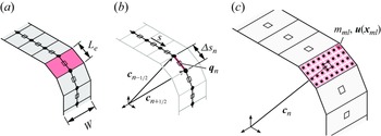


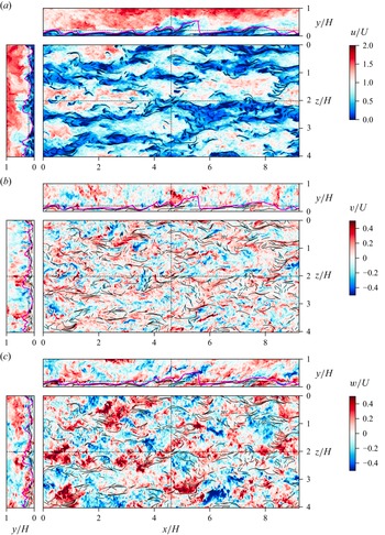


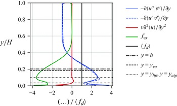


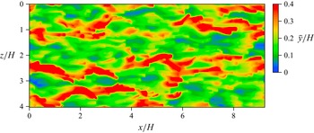


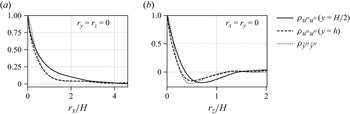


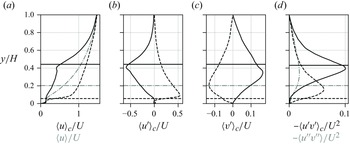


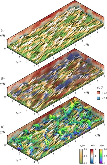


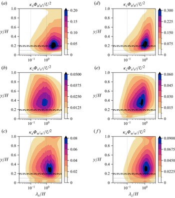


 Open access

